Nash Equilibrium and Learning Dynamics
in Three-Player Matching $m$-Action Games

Abstract

Learning in games discusses the processes where multiple players learn their optimal strategies through the repetition of game plays. The dynamics of learning between two players in zero-sum games, such as matching pennies, where their benefits are competitive, have already been well analyzed. However, it is still unexplored and challenging to analyze the dynamics of learning among three players. In this study, we formulate a minimalistic game where three players compete to match their actions with one another. Although interaction among three players diversifies and complicates the Nash equilibria, we fully analyze the equilibria. We also discuss the dynamics of learning based on some famous algorithms categorized into Follow the Regularized Leader. From both theoretical and experimental aspects, we characterize the dynamics by categorizing three-player interactions into three forces to synchronize their actions, switch their actions rotationally, and seek competition.

1 Introduction

Learning in games considers that multiple agents independently learn their strategies to increase their utility [Fudenberg and Levine, 1998]. How to achieve the Nash equilibrium [Nash Jr, 1950], in which all agents are not motivated to change their strategies, is a key issue in learning in games. However, this issue is critical when their utility functions conflict with each other. The minimum example of such a conflict is matching pennies, where two agents have two actions, and their optimal actions are interdependent on each other, i.e., conflict.

To resolve this issue, the dynamics of agents’ strategies have been enthusiastically studied in recent years [Tuyls and Nowé, 2005, Tuyls et al., 2006, Bloembergen et al., 2015]. A representative method to analyze the dynamics is the learning algorithm named Follow the Regularized Leader (FTRL) [Shalev-Shwartz and Singer, 2006, Mertikopoulos and Sandholm, 2016, Mertikopoulos et al., 2018], including several well-known algorithms, such as replicator dynamics [Taylor and Jonker, 1978, Friedman, 1991, Hofbauer et al., 1998, Börgers and Sarin, 1997, Hofbauer et al., 1998, Sato et al., 2002] and gradient ascent [Hofbauer and Sigmund, 1990, Dieckmann and Law, 1996, Singh et al., 2000, Zinkevich, 2003]. The above matching pennies game attracts a lot of attention to discuss the dynamics, where their strategies draw a cycle around the Nash equilibrium [Börgers and Sarin, 1997, Bloembergen et al., 2015]. Such cycling dynamics are also observed in some variations of games [Hofbauer et al., 1998, Singh et al., 2000, Bailey and Piliouras, 2019] derived from the matching pennies and are understood by a conserved quantity [Piliouras et al., 2014, Mertikopoulos et al., 2018, Bailey and Piliouras, 2019]. As a topic developing recently, various algorithms are proposed and achieve the convergence to the Nash equilibrium (called last-iterate convergence), especially in games that usually result in cycles [Bowling, 2000, Anagnostides et al., 2022, Fujimoto et al., 2024], where their payoff matrices can be separated into interactions between pairs of players. To summarize, analyzing the cycling dynamics of agents’ strategies matters in learning in games, where the matching pennies game is a keystone.

Despite such a thorough understanding of two-player games, three-player games are still little explored. Jordan’s game is proposed as a three-player version of the matching pennies [Jordan, 1993]. Several studies discussed learning dynamics (mainly based on fictitious play [Brown, 1951]) in this game [Gaunersdorfer and Hofbauer, 1995, McCabe et al., 2000, Shamma and Arslan, 2005, Mealing and Shapiro, 2015], where divergence from the Nash equilibrium is observed. Considering the observed cycling dynamics in the matching pennies game and its variants, it can be anticipated that certain three-player interactions may qualitatively alter learning dynamics. However, how three-player interaction can change the structure of the game (e.g., the region of Nash equilibrium and the global behavior of learning dynamics) is still unclear in general. Indeed, few but some studies support that such three-player interaction complicates dynamics in three-player rock-paper-scissors [Sato et al., 2005] and social dilemma [Akiyama and Kaneko, 2000] and also makes it hard to calculate equilibrium strategies in rock-paper-scissors [Grant, 2023], social dilemma [Murase and Baek, 2018], and Kuhn poker [Szafron et al., 2013]. It also should be remarked that game AIs are developing rapidly in several multi-player table games, including Poker [Brown and Sandholm, 2019], Mahjong [Li et al., 2020], and Diplomacy [Paquette et al., 2019]. To summarize, understanding how three-player interactions change the game structure is crucial for gaining better insight into a variety of three-player games.

This study extends the ordinary matching pennies game to a three-player general $m$-action version and name it Three-Player Matching $m$-Action ($m$-3MA) game. We first derive all the Nash equilibria in $m$-3MA and show that the equilibria are diverse and complicated depending on the parameters of three-player interaction. Furthermore, we introduce the continuous-time FTRL algorithm. Next, we analyze the dynamics of this algorithm in $m$-3MA for several representative regularizers, i.e., the entropic and Euclidean ones. We observe that the dynamics provide various behaviors depending on the parameters of three-player interaction: cycle around the Nash equilibria, convergence to there, and divergence to a heteroclinic cycle. We further introduce a novel quantity which is the degree of synchronization among three players’ actions, and prove that this quantity captures the global behavior of the dynamics in some cases.

2 Preliminary

2.1 Three-Player Matching $m$-Action Games

We now assume a situation where one’s action is advantageous under a certain pair of the others’ actions but is disadvantageous under another pair. Thus, the property of the matching pennies game is inherited. Based on this situation, we now formulate Three-Player Matching $m$-Action ($m$-3MA) games.

Let X, Y, and Z denote three players. Every round, they independently determine their actions from the same $m$-action set, $\mathcal{A}=\{a_{1},\cdots,a_{m}\}$ (see Fig. 1-A). Players who choose the same action interact with each other. This interaction follows a three-way deadlock relationship among them (see Fig. 1-B): X wins Y, Y wins Z, but Z wins X. They receive their scores (see Fig. 1-C). When only two of them interact, the winner and loser are determined following the three-way deadlock relationship, and the winner’s and loser’s scores are $a$ and $b$ (see the left panel of Fig. 1-C), respectively. Players who chose a different action from the others receive the default payoff of $c$ (see the center). If all three players take the same action, they commonly receive the scores of $\epsilon$ (see the right). Here, we assume that the winner’s and loser’s scores are highest and lowest, respectively, i.e., $b<c<a$ and $b<\epsilon<a$.

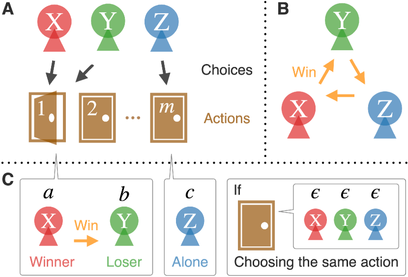
Figure 1: A. Three players, X, Y, and Z, independently choose their actions. Players who choose the same action play the game together. B. In the game, players have a three-way deadlock relationship. X, Y, and Z are advantageous to Y, Z, and X, respectively. C. The three players receive their own scores as a result of their action choices. When two of the three players (X and Y in the left panel) choose the same action, the winner’s score is $a$, while the loser’s score is $b$, following the three-way deadlock relationship. An isolated player (Z in the center panel) who chooses a different action from others receives a score of $c$. If all three players choose the same action (in the right panel), they receive scores of $\epsilon$. Here, we assume $b<c<a$ and $b<\epsilon<a$.

We also formulate their mixed strategies and payoffs. Let $0\leq x_{i}\leq 1$ denote the probability that X chooses action $a_{i}$. X’s strategy is defined as $\bm{x}:=(x_{1},\cdots,x_{m})\in\Delta^{m-1}$ (the $m-1$ dimensional simplex). Similarly, Y’s and Z’s strategies are denoted by $\bm{y}\in\Delta^{m-1}$ and $\bm{z}\in\Delta^{m-1}$, respectively. When players follow such strategies, X’s expected payoff is given by

$$u(\bm{x},\bm{y},\bm{z}) =\epsilon\sum_{i}x_{i}y_{i}z_{i}+a\sum_{i}x_{i}y_{i}\bar{z}_{i}$$

$$+b\sum_{i}x_{i}\bar{y}_{i}z_{i}+c\sum_{i}x_{i}\bar{y}_{i}\bar{z}_{i},$$ (1)

where we defined $\bar{\mathcal{X}}:=1-\mathcal{X}$ for arbitrary variable $\mathcal{X}$. Y’s and Z’s expected payoffs are also described as $u(\bm{y},\bm{z},\bm{x})$ and $u(\bm{z},\bm{x},\bm{y})$, respectively.

In learning in games, the gradient of this payoff is often important, calculated as

$$\frac{\partial u(\bm{x},\bm{y},\bm{z})}{\partial x_{i}}$$

$$=\epsilon y_{i}z_{i}+ay_{i}\bar{z}_{i}+b\bar{y}_{i}z_{i}+c\bar{y}_{i}\bar{z}_{i},$$

$$=(\epsilon-a-b+c)y_{i}z_{i}+(a-c)y_{i}+(b-c)z_{i}+c,$$

$$=(\alpha-\gamma)y_{i}z_{i}+\frac{\beta+\gamma}{2}y_{i}+\frac{-\beta+\gamma}{2}z_{i}+c,$$

$$=:f(y_{i},z_{i}),$$ (2)

where we define $\alpha:=\epsilon-c$, $\beta:=a-b>0$, and $\gamma:=a+b-2c$. In this payoff gradient, $c$ is the offset and thus negligible. Thus, we can characterize the $m$-3MA games by the three parameters of $\alpha$, $\beta$, and $\gamma$.

3 Nash Equilibrium

The Nash equilibrium of $m$-3MA is defined as the set of strategies $(\bm{x}^{*},\bm{y}^{*},\bm{z}^{*})$ that satisfy

$$\begin{cases}\bm{x}^{*}\in\arg\max_{\bm{x}}u(\bm{x},\bm{y}^{*},\bm{z}^{*})\\ \bm{y}^{*}\in\arg\max_{\bm{y}}u(\bm{y},\bm{z}^{*},\bm{x}^{*})\\ \bm{z}^{*}\in\arg\max_{\bm{z}}u(\bm{z},\bm{x}^{*},\bm{y}^{*})\\ \end{cases}.$$ (3)

It is difficult to derive equilibrium in three-player games [Daskalakis and Papadimitriou, 2005], and indeed, there are few successful studies [Szafron et al., 2013, Grant, 2023]. Nevertheless, we can fully analyze all the Nash equilibria in Thm. 1 in Sec. 3.1. Because the theorem is based on rigorous but complicated calculations, its visualization and brief interpretation are provided in Sec. 3.2.

3.1 Full Analysis

We first introduce three types of strategies consisting of the Nash equilibrium. The first is the uniform-choice equilibrium $\mathcal{N}_{\rm U}(m):=\{\bm{1}/m\}$, where $\bm{1}$ is defined as the $m$-dimensional all-ones vector. In this equilibrium, the player chooses all the actions at perfectly random. The second is the pure-strategy equilibria $\mathcal{N}_{\rm P}(m):=\{\bm{e}_{1},\cdots,\bm{e}_{m}\}$, where $\bm{e}_{i}$ is the unit vector for the $i$-th axis in the $m$-dimensional space. These equilibria mean that the player deterministically chooses an action (uses a pure strategy). The third is the double roots equilibria;

$$\mathcal{N}_{\rm DR}(m):=\begin{cases}\{\sigma(\bm{x}_{{\rm DR};k})\;|\;\sigma\in S_{m},k\leq 1/(2x_{{\rm ext}})\}\\ \hskip 85.35826pt(x_{{\rm ext}}>1/m)\\ \{\sigma(\bm{x}_{{\rm DR};k})\;|\;\sigma\in S_{m},k\geq 1/(2x_{{\rm ext}})\}\\ \hskip 85.35826pt(x_{{\rm ext}}<1/m)\\ \end{cases},$$ (4)

where we used the permutation function $\sigma$ for $m$-dimensional symmetry group $S_{m}$, and also used

$$x_{{\rm ext}} :=\frac{\gamma}{2(\gamma-\alpha)},$$ (5)

$$\delta :=\frac{mx_{{\rm ext}}-1}{m-2k},$$ (6)

$$x_{+} :=x_{{\rm ext}}+\delta,$$ (7)

$$x_{-} :=x_{{\rm ext}}-\delta,$$ (8)

$$\bm{x}_{{\rm DR};k} :=(\underbrace{x_{+},\cdots,x_{+}}_{k},\underbrace{x_{-},\cdots,x_{-}}_{m-k}).$$ (9)

These equilibria are very complex because the player chooses each action with two different probabilities $x_{+}$ and $x_{-}$.

In addition, for the range of $A=\{2,\cdots,m-1\}$, we define

$$\mathcal{N}^{\prime}_{\rm U}(m) :=\mathcal{N}_{\rm U}(m)\cup\left(\bigcup_{m^{\prime}\in A}\mathrm{Proj}^{-1}(\mathcal{N}_{\rm U}(m^{\prime}))\right),$$ (10)

where $\mathrm{Proj}^{-1}$ denotes an inverse projection map from $m^{\prime}(<m)$- to $m$-dimensional vector set with arbitrary permutations. Thus, $\mathcal{N}^{\prime}_{\rm U}(m)$ contains all the uniform-choice equilibria of $m^{\prime}(<m)$-action games. Here, we split $A$ into $A^{(-)}:=\{2,\cdots,\lfloor 1/(2x_{{\rm ext}})\rfloor\}$ and $A^{(+)}:=\{\lceil 1/(2x_{{\rm ext}})\rceil,\cdots,m-1\}$ as $A=A^{(-)}\cup A^{(+)}$. Then, $\mathcal{N}^{\prime(-)}_{\rm U}(m)$ (resp. $\mathcal{N}^{\prime(+)}_{\rm U}(m)$) denotes that the union set in the range of $m^{\prime}\in A^{(-)}$ (resp. $A^{(+)}$). $\mathcal{N}^{\prime}_{\rm DR}(m)$ is similarly defined.

Using the above definition, we derive the Nash equilibria as follows.

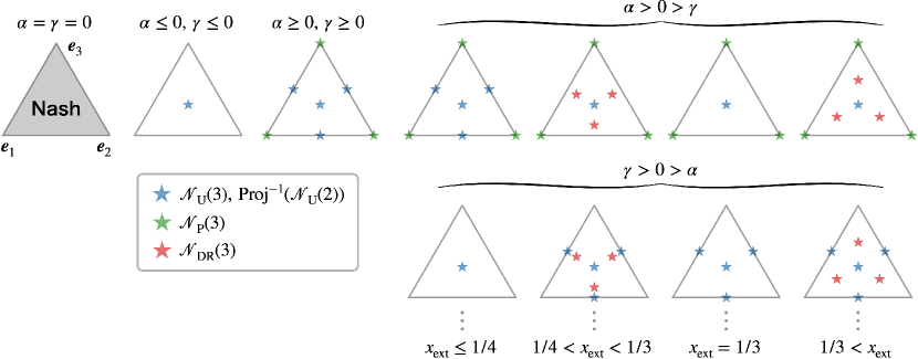
Figure 2: The Nash equilibrium in $m$-3MA with $m=3$. This Nash equilibrium crucially changes depending on $\alpha$ and $\gamma$. Each panel shows the simplex $\Delta^{2}$ of one’s strategy. The edges of triangles indicate the pure strategies, i.e., $\bm{x}=\bm{y}=\bm{z}=\bm{e}_{i}$, where all the players choose only action $i$. The blue stars represent $\mathcal{N}_{\rm U}(3)$ (and $\mathrm{Proj}^{-1}(\mathcal{N}_{\rm U}(2))$). The green stars represent $\mathcal{N}_{\rm P}(3)$. Finally, the red stars represent $\mathcal{N}_{\rm DR}(3)$. Here, note that since we consider the case of $m=3$, $\mathrm{Proj}^{-1}(\mathcal{N}_{\rm DR}(2))=\emptyset$ always hold. Here, the positions of $\mathcal{N}_{\rm DR}$ change depending on $x_{{\rm ext}}$, which is determined by $\alpha$ and $\gamma$.

Theorem 1 (Nash equilibrium solution).

For any Nash equilibrium $(\bm{x}^{*},\bm{y}^{*},\bm{z}^{*})$, $\bm{x}^{*}=\bm{y}^{*}=\bm{z}^{*}$ holds, and the set of one’s strategies is given by

$$\begin{cases}\alpha=\gamma=0&\Rightarrow\Delta^{m-1}\\ 0\geq\alpha,0\geq\gamma&\Rightarrow\mathcal{N}_{\rm U}(m)\\ \alpha>0>\gamma&\Rightarrow\mathcal{N}_{\rm P}(m)\cup\mathcal{N}^{\prime(-)}_{\rm U}(m)\cup\mathcal{N}_{\rm DR}(m)\\ \alpha\geq 0,\gamma\geq 0&\Rightarrow\mathcal{N}_{\rm P}(m)\cup\mathcal{N}^{\prime}_{\rm U}(m)\\ \gamma>0>\alpha&\Rightarrow\mathcal{N}_{\rm U}^{\prime(+)}(m)\cup\mathcal{N}^{\prime}_{\rm DR}(m)\end{cases}.$$ (11)

See Appendix. A.1-A.4 for its complete proof.

Proof Sketch. Step 1 (Lemma 4): We prove $\bm{x}^{*}=\bm{y}^{*}=\bm{z}^{*}$ by contradiction. In other words, we derive a contradiction from the assumption of $\bm{x}^{*}\neq\bm{y}^{*}\neq\bm{z}^{*}\neq\bm{x}^{*}$ or $\bm{x}^{*}=\bm{y}^{*}\neq\bm{z}^{*}$. This contradiction is proved because there is no ordering among $f(y_{i}^{*},z_{i}^{*})$, $f(z_{i}^{*},x_{i}^{*})$, and $f(x_{i}^{*},y_{i}^{*})$. Step 2 (Lemma 5 and 6): Under the condition of $\bm{x}^{*}=\bm{y}^{*}=\bm{z}^{*}$, we find the set of one’s equilibrium strategies. Both the cases when its strategy exists in the interior or on the boundary of the strategy spaces are considered. ∎

3.2 Visualization and Interpretation

To visualize Thm. 1, Fig. 2 illustrates all the cases of the Nash equilibria. As this figure shows, $m$-3MA provides diverse and complicated Nash equilibrium structures depending on $\alpha$ and $\gamma$. The Nash equilibria are especially complicated when $\alpha$ and $\gamma$ conflict (i.e., $\alpha>0>\gamma$ or $\gamma>0>\alpha$). For further interpretation of the Nash equilibria, the following corollary summarizes the main properties of the equilibria.

Corollary 1 (Main properties of the Nash equilibria).

First, the following property always holds.

• (Player symmetry) For any Nash equilibrium, all three players take the same strategy, i.e., $\bm{x}^{*}=\bm{y}^{*}=\bm{z}^{*}$.

Furthermore, the region of the Nash equilibria has the following properties.

• (Neutral equilibria) When $\alpha=\gamma=0$, all the strategies in the simplex $\Delta^{m-1}$ can be the Nash equilibria.

• (Pure-strategy equilibria) $\mathcal{N}_{\rm P}(m)=\{\bm{e}_{1},\cdots,\bm{e}_{m}\}$ are the Nash equilibrium strategies, if and only if $\alpha\geq 0$.

• (Uniform-choice equilibrium) $\mathcal{N}_{\rm U}(m)=\{\bm{1}/m\}$ is always the Nash equilibrium strategy.

Proof. These properties are immediately derived by Thm. 1. ∎

We now interpret these properties of the Nash equilibria. (Neutral equilibrium) The games with $\alpha=\gamma=0$ are classified as a zero-sum game which satisfies monotonicity. Thus, no three-body effect works, and a continuous region can be equilibrium. (Pure-strategy equilibria) The games with $\alpha>0$ have a positive three-body effect, where positive payoffs are generated when three players interact. In such games, the players are motivated to synchronize their actions. Thus, the states in which the three players perfectly synchronize their action choices, i.e., the pure-strategy equilibria, can be equilibrium. (Uniform-choice equilibrium) When the other two players take all actions at perfectly random, i.e., use $\bm{1}/m$, all the actions are equivalent for a player. Thus, the uniform-choice equilibrium $\bm{x}^{*}=\bm{y}^{*}=\bm{z}^{*}=\mathcal{N}_{\rm U}(m)$ is always the Nash equilibrium independent of $\alpha$.

4 Continuous-Time Follow the Regularized Leader

This study considers the continuous-time Follow the Regularized Leader (FTRL), which is formulated as

$$\bm{x} =\bm{q}(\bm{x}^{\dagger}),$$ (12)

$$\dot{\bm{x}}^{\dagger} =\frac{\partial u}{\partial\bm{x}},$$ (13)

$$\bm{q}(\bm{x}^{\dagger}) =\arg\max_{\bm{x}}\left\{\bm{x}^{\dagger}\cdot\bm{x}-h(\bm{x})\right\}.$$ (14)

Here, $h(\bm{x})$ is called the “regularizer”. Several representative examples of this regularizer are the entropic regularizer $h(\bm{x})=\bm{x}\cdot\log\bm{x}$ and the Euclidean regularizer $h(\bm{x})=\|\bm{x}\|^{2}/2$. The following lemma shows that these regularizers provide the replicator dynamics and gradient ascent, based on the result in [Mertikopoulos et al., 2018].

Lemma 1 (Replicator dynamics and gradient ascent).

(Replicator dynamics) In $m$-3MA, the continuous-time FTRL with $h(\bm{x})=\bm{x}\cdot\log\bm{x}$ are calculated as

$$\dot{x}_{i}= x_{i}\left(f(y_{i},z_{i})-\sum_{i}x_{i}f(y_{i},z_{i})\right).$$ (15)

(Gradient ascent) In the interior of the players’ strategy spaces, the continuous-time FTRL with $h(\bm{x})=\|\bm{x}\|^{2}/2$ are calculated as

$$\dot{x}_{i}= f(y_{i},z_{i})-\frac{1}{m}\sum_{i}f(y_{i},z_{i}).$$ (16)

5 Learning Dynamics

Let us consider learning dynamics by continuous-time FTRL. In Sec. 5.1, two quantities, $G$ and $V$, are introduced to characterize the learning dynamics. In Sec. 5.2, we theoretically analyze the global behavior of the learning dynamics by using $G$ and $V$. Finally, in Secs. 5.2 and 5.3, we simulate the learning dynamics for $m=2$ and $m>2$ and experimentally demonstrate how game parameters, i.e., $\alpha$, $\beta$, and $\gamma$, contribute to the dynamics.

5.1 Characterization of $m$-3MA

To investigate learning dynamics given by the continuous-time FTRL, we introduce $G$ and $V$ as

$$G(\bm{x}^{\dagger},\bm{y}^{\dagger},\bm{z}^{\dagger}) :=\Sigma_{\rm cyc}\ \max_{\bm{x}}\{\bm{x}^{\dagger}\cdot\bm{x}-h(\bm{x})\}-\bm{x}^{\dagger}\cdot{\color[rgb]{0,0,0}\bm{1}/m},$$ (17)

$$V(\bm{x},\bm{y},\bm{z}) :=\Sigma_{i}\ x_{i}y_{i}z_{i}-1/m^{2}.$$ (18)

Here, $\Sigma_{\rm cyc}\$ indicates the cyclic sum for three players. In other words, $\Sigma_{\rm cyc}\ \mathcal{F}(\bm{x})=\mathcal{F}(\bm{x})+\mathcal{F}(\bm{y})+\mathcal{F}(\bm{z})$ holds for arbitrary function $\mathcal{F}$. We now explain the meanings of $G$ and $V$. First, $G$ is known to be conserved under zero-sum games [Mertikopoulos et al., 2018] and corresponds to Kullback-Leibler divergence from the uniform-choice equilibrium. Next, $V$ means the probability that all three players choose the same action, in other words, the degree of synchronization of their action choices. The following lemma gives the basics of this $V$;

Lemma 2 (Properties of $V$).

$V$ takes its maximum value if and only if $\bm{x}=\bm{y}=\bm{z}\in\mathcal{N}_{\rm P}(m)$ and its minimum value if and only if $x_{i}=0$, $y_{i}=0$, or $z_{i}=0$ hold for each $i\in\{1,\cdots,m\}$.

Proof. For the maximum value condition, $\Sigma_{i}\ x_{i}y_{i}z_{i}\leq\sum_{i}x_{i}y_{i}\leq 1$ trivially holds. The second equation holds if and only if $\bm{x}=\bm{y}\in\mathcal{N}_{\rm P}(m)$ by the definition of an inner product. The first equation further holds if and only if $\bm{x}=\bm{y}=\bm{z}\in\mathcal{N}_{\rm P}(m)$. For the minimum value condition, $0\leq\Sigma_{i}\ x_{i}y_{i}z_{i}$ trivially holds. Here, this equation holds if and only if $x_{i}y_{i}z_{i}=0\Leftrightarrow(x_{i}=0)\lor(y_{i}=0)\lor(z_{i}=0)$ for all $i\in\{1,\cdots,m\}$. ∎

5.2 Analysis and Experiments of Two-Action Games

5.2.1 Theoretical Analysis

We now consider $m$-3MA with the case of $m=2$. Since $m=2$ holds, $x_{2}=1-x_{1}$, $y_{2}=1-y_{1}$, and $z_{2}=1-z_{1}$ hold so that we can describe the learning dynamics by the three variables of $(x_{1},y_{1},z_{1})$. The dynamics given by the FTRL algorithm in the game are independent of $\gamma$, as proved in the following.

Lemma 3 (Simplified dynamics for $m=2$).

When $m=2$, the dynamics in Lem. 1 are calculated as

$$\dot{x}_{1} =w(x_{1})\{\alpha(y_{1}+z_{1}-1)+\beta(y_{1}-z_{1})\},$$ (19)

$$w(x_{1}) =\begin{cases}x_{1}(1-x_{1})&(h(\bm{x})=\bm{x}\cdot\log\bm{x})\\ 1/2&(h(\bm{x})=\|\bm{x}\|^{2}/2)\\ \end{cases},$$ (20)

independent of $\gamma$.

See Appendix. A.5 for its complete proof.

Proof Sketch. Since $x_{2}=\bar{x}_{1}$, $y_{2}=\bar{y}_{1}$, and $z_{2}=\bar{z}_{1}$ hold in two-action games, the dynamics in Lem. 1 are rewritten in a simpler form by direct calculation. ∎

Under the entropic and Euclidean regularizers, the time changes of these $V$ and $G$ are characterized by the following two theorems.

Theorem 2 (Monotonicity of $V$).

In $m$-3MA with $m=2$, the FTRL algorithm with the entropic regularizer $h(\bm{x})=\bm{x}\cdot\log\bm{x}$ and Euclidean reguralizer $h(\bm{x})=\|\bm{x}\|^{2}/2$ gives

$${\rm sign}(\dot{V})={\rm sign}(\alpha),$$ (21)

in the interior of strategy space other than $\bm{x}=\bm{y}=\bm{z}=\bm{1}/m$.

See Appendix. A.6 for its complete proof.

Proof Sketch. We calculate the dynamics of $V$ by using Eq. (19). The two terms of $\alpha$ and $\beta$ contribute to the dynamics. Here, the term of $\beta$ disappears by the cyclic symmetry among the three players. The term of $\alpha$ is always positive, meaning that the signs of $\dot{V}$ and $\alpha$ are the same. ∎

Theorem 3 (Connection between $G$ and $V$).

In $m$-3MA with $m=2$, the FTRL algorithm with the entropic regularizer $h(\bm{x})=\bm{x}\cdot\log\bm{x}$ and Euclidean reguralizer $h(\bm{x})=\|\bm{x}\|^{2}/2$ gives $\dot{G}=2\alpha V$ in the interior of strategy space other than $\bm{x}=\bm{y}=\bm{z}=\bm{1}/m$.

See Appendix. A.7 for its complete proof.

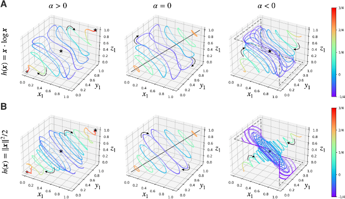
Figure 3: A. The dynamics of FTRL with the entropic regularizer in $m$-3MA with $m=2$. The dynamics are output by the fourth-order Runge-Kutta method with the step-size of $2\times 10^{-2}$ in all the panels. We also commonly set $(a,b,c)=(1,-1,0)$, in other words, $\beta=2$. In the left, center, and right panels, we set $\epsilon(=\alpha)=0.1$, $0$, $-0.1$, respectively. The red, green, and blue lines indicate the time series of $x_{i}$, $y_{i}$, and $z_{i}$, respectively, while the solid, broken, and dotted lines indicate $i=1$, $2$, and $3$, respectively. The solid black line indicates the time series of $V$. The initial strategies in each panel are randomly sampled from the strategy simplexes. In the left and right panels, the Nash equilibria are plotted by the black star. In the center panel, all the points on the black solid line are the Nash equilibria. The broken line in the right panel is the set of states satisfying the minimum $V$ condition. B. The dynamics of FTRL with the Euclidean regularizer. The method and simulation parameters are the same as panel A.

Proof Sketch. The dynamics of $G$ are calculated by using Eq. (19) and depend on both $\alpha$ and $\beta$. Here, the term of $\beta$ disappears again by the cyclic symmetry among the three players. The term of $\alpha$ corresponds to $2V$. ∎

These two theorems explain the global behavior of the learning dynamics as follows.

Corollary 2 (Global behavior of dynamics).

In $m$-3MA with $m=2$, the continuous-time FTRL gives the following properties except for when the trajectory converges to the uniform-choice equilibrium.

• When $\alpha=0$, both $G$ and $V$ are conserved in the trajectory.

• When $\alpha>0$, the trajectory asymptotically converges to the states of maximum $V$, i.e., either of the fixed points.

• When $\alpha<0$, the trajectory asymptotically converges to the states of minimum $V$, i.e., the heteroclinic cycle.

Proof. This is immediately proved by Lem. 2, Thm. 2, and Thm. 3.

5.2.2 Experimental Understanding

We numerically demonstrate the learning trajectories in $m$-3MA with $m=2$. Fig. 3-A and B show the learning dynamics by continuous-time FTRL with the entropic (replicator dynamics) and Euclidean (gradient ascent) regularizers, respectively. Each figure plots the dynamics in the three cases of $\alpha>0$ (left), $\alpha=0$ (center), and $\alpha<0$ (right). One can see some differences between Fig. 3-A and B. The trajectory of the replicator dynamics has a distorted shape and always stays in the interior of the strategy space. On the other hand, the trajectory of the gradient ascent has a circular shape and often stays on the boundary of the strategy space. Regardless of such a difference, the trajectory commonly shows the properties given by Cor. 2 as follows.

Cycling behavior ($\alpha=0$):

First, we see the case of $\alpha=0$. Thm. 1 shows that the Nash equilibria are given by the diagonal line of $\bm{x}^{*}=\bm{y}^{*}=\bm{z}^{*}\in\Delta^{1}$. Then, the learning dynamics always give cycling behavior around this diagonal line. As Cor. 2 proves, both $G$ and $V$ are invariant. Indeed, we can see that $V$ is constant in each trajectory (plotted by the same color), while $G$, the distance from the uniform-choice equilibrium in the center point, also seems constant in each trajectory.

Convergence to the pure-strategy equilibria ($\alpha>0$):

In $\alpha>0$, the Nash equilibria are given by $\bm{x}^{*}=\bm{y}^{*}=\bm{z}^{*}\in\mathcal{N}_{\rm P}(2)\cup\mathcal{N}_{\rm U}(2)=\{\bm{e}_{1},\bm{e}_{2},\bm{1}/2\}$. As Cor. 2 proves, the learning dynamics converge to either one of the pure-strategy equilibria $\bm{e}_{1}$ or $\bm{e}_{2}$ depending on their initial condition. Indeed, we can see that $V$ monotonically increases in each trajectory (the plotted color changes into red monotonically).

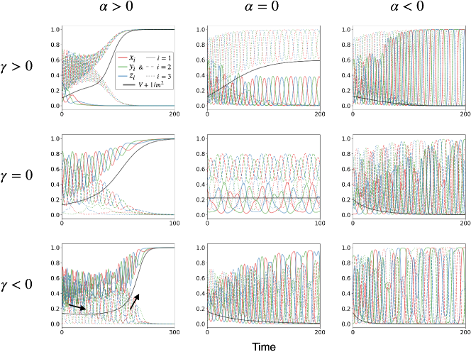
Figure 4: The dynamics of FTRL with the entropic regularizer. The dynamics are output by the fourth-order Runge-Kutta method with the step-size of $2\times 10^{-2}$ in all the panels. For $\alpha>0$, $=0$, and $<0$, we set $(\epsilon,c)=(0.1,0)$, $(0,0)$, and $(-0.1,0)$, respectively. For $\gamma>0$, $=0$, and $<0$, we set $(a,b,c)=(1.1,-0.9,0)$, $(1,-1,0)$, and $(0.9,-1.1,0)$, respectively.

Heteroclinic cycles ($\alpha<0$):

In $\alpha<0$, the Nash equilibrium is only at $\bm{x}^{*}=\bm{y}^{*}=\bm{z}^{*}\in\mathcal{N}_{\rm U}(2)=\{\bm{1}/2\}$. Interestingly, the learning dynamics do not reach this Nash equilibrium but converge to the heteroclinic cycle of $(x_{1},y_{1},z_{1})=(0,0,1)\to(0,1,1)\to(0,1,0)\to(1,1,0)\to(1,0,0)\to(1,0,1)\to(0,0,1)\to\cdots$. This means that as each player cyclically changes his/her action, he/she more biasedly chooses the action. In this heteroclinic cycle, $V$ takes its minimum value, and thus it is observed that Cor. 2 holds. The uniform-choice equilibrium $\bm{1}/2$ is unstable and cannot be reached from almost all the initial conditions.

$\alpha$ is the force of synchronization:

Let us explain the convergence in $\alpha>0$ and the divergence to the heteroclinic cycle in $\alpha<0$. Consider whether a player should choose the same action as the two others. If choosing, the player obtains $\epsilon$. Otherwise, $c$. In $\alpha>0\Leftrightarrow\epsilon>c$, the three players prefer to synchronize their actions more, eventually concentrating on choosing either action. On the other hand, in $\alpha<0\Leftrightarrow\epsilon<c$, the players prefer to desynchronize their actions.

$\beta$ is the force of rotation:

We also interpret $\beta=a-b$. Here, $a(>0)$ is the score for a winner. Thus, the larger $a$ is, the more quickly players are motivated to learn an advantageous action. On the other hand, $b(<0)$ is the score for a loser. The smaller $b$ means that players quickly learn to escape from being exploited. Because three players have a three-way deadlock relationship, their strategies show rotation. $\beta$ indicates the force of rotation.

5.3 Experiments of More than Two-Action Games

Next, we consider $m$-3MA with $m>2$, where the learning dynamics are more complicated than the case of $m=2$. Now, Fig. 4 shows that these dynamics are classified by not only $\alpha$ but $\gamma$.

Conservation of action number ($\gamma=0$)

: Let us consider the case of $\gamma=0$ (see the three panels in the middle row of Fig. 4). This case is viewed as the extension of the above dynamics to general $m>2$. In other words, when $\alpha=0$, the learning dynamics show a cycling behavior. When $\alpha>0$, players synchronize their actions throughout the learning: convergence to the pure-strategy equilibria, i.e., $\mathcal{N}_{\rm P}(m)$, depending on their initial strategies. When $\alpha<0$, players learn to desynchronize their actions and cannot reach the only uniform-choice equilibrium. These various dynamics are characterized by $V=\sum_{i}x_{i}y_{i}z_{i}-1/m^{2}$, again. In mathematics, we obtain the following theorem.

Theorem 4 (Monotonicity of $V$ for $m$-3MA).

In the replicator dynamics in Lem. 1, except for the uniform-choice equilibrium $\bm{x}=\bm{y}=\bm{z}\in\mathcal{N}_{\rm U}(m)$, ${\rm sign}(\dot{V})={\rm sign}(\alpha)$ holds.

See Appendix. A.8 for its complete proof.

Proof Sketch. We calculate $\dot{V}$ by substituting Eq. (15). Because $\gamma$ is ignored, only the terms of $\alpha$ and $\beta$ contribute to the dynamics. Here, the term of $\beta$ is negligible by the cyclic symmetry among the three players. Furthermore, the term of $\alpha$ is described as the variance of $y_{i}z_{i}$, which is positive everywhere except for $\bm{x}=\bm{y}=\bm{z}\in\mathcal{N}_{\rm U}(m)$. ∎

Convergence to two-action games ($\gamma>0$):

We next see the case of $\gamma>0$ (see the three panels in the upper row of Fig. 4). The dynamics approach those in the two-action games. As a simple example, see the dynamics in $\alpha=0$. Near the initial time, all players take all three actions stochastically. Throughout learning, however, one of the three actions ($a_{2}$ in the panel) becomes not played at all. Eventually, all players learn to use only the other two actions oscillatory. In other words, the three-action game converges to a two-action game after a sufficiently long time. The cases of $\alpha\neq 0$ can be interpreted similarly. In $\alpha>0$, the players first learn not to use one of three actions ($a_{1}$ in the panel) and synchronize their actions after that. In $\alpha<0$, players first learn not to use one action ($a_{2}$ in the panel) and finally reach a heteroclinic cycle.

Divergence to $m$-actions games ($\gamma<0$):

We finally see the case of $\gamma<0$ (see the three panels in the lower row of Fig. 4). The three players basically learn to desynchronize their actions. Indeed, the lower-middle and lower-right panels are similar to the middle-right panel ($\gamma=0,\alpha<0$). The case of $\gamma<0,\alpha>0$ is an exception. In this case, three players first desynchronize their actions (i.e., $V$ decreases in the lower-left panel), but synchronize their actions in the end (i.e., $V$ conversely increases). Because $\alpha(>0)$ and $\gamma(<0)$ conflict in this case, non-monotonic dynamics of $V$ are clearly observed. Whether their actions eventually synchronize or desynchronize depends on the initial condition.

$\gamma$ is the force to seek competition:

We now interpret another three-player interaction, $\gamma=a+b-2c$. First, note that in games with more than two actions, three players do not have to interact, i.e., they may choose different three actions separately. When two of the players compete with each other, i.e., choose the same action, the three players totally obtain the payoff of $a+b+c$. On the other hand, when they choose different three actions, their total payoff is $3c$. Thus, $\gamma>0\Leftrightarrow a+b+c>3c$ means that the players expectedly obtain higher payoffs when they compete. In this meaning, they, over time, learn to compete more often and to cyclically choose only two of $m$ actions. On the other hand, in $\gamma<0$, they learn to avoid competition as much as possible, leading to the dispersion of their action choices.

6 Conclusion

Three-player games are still much unexplored, compared to two-player games. This study focused on how three-player interactions affect the games. Surprisingly, we fully analyzed the Nash equilibria, even though solving the Nash equilibria of three-player games is sufficiently difficult in general [Chen and Deng, 2006, Daskalakis et al., 2009]. We also found that the Nash equilibria are various and complex Nash equilibria when three-player interactions, i.e., $\alpha$ and $\gamma$, conflict. Such three-player interactions also complicate the learning dynamics: The conserved quantities in a constant-sum game are no longer robust for such three-player interaction. We found the Lyapunov function $V$ and proved that $V$ monotonically increases or decreases depending on $\alpha$. We further demonstrated by simulation that learning dynamics can be classified by $\alpha$, the force to synchronize the choices of three players, and $\gamma$, the preference for competition with others. In conclusion, this study showed theoretical analyses and experimental findings regarding three-player interaction to the maximum.

How to achieve convergence to the Nash equilibrium, called last-iterate convergence, in three-player games is a topic of great interest. Recent literature shows that the FTRL achieves convergence to the Nash equilibrium in two-player zero-sum games when it optimistically foresees its opponent’s future strategy [Mertikopoulos et al., 2019, Daskalakis and Panageas, 2019] or incorporates mutations into its learning [Abe et al., 2022, 2023]. In addition, memory, i.e., the ability to change one’s action depending on the past games, is known to change game structures. For example, this memory extends the region of the Nash equilibrium [Fujimoto and Kaneko, 2019, 2021, Usui and Ueda, 2021, Ueda, 2023], induces divergence [Fujimoto et al., 2023], and achieves convergence [Fujimoto et al., 2024]. It would be interesting future works to see how these learning algorithms perform in three-player games. This study will provide both a theoretical and experimental basis for such future works.

Appendix of: Nash Equilibrium and Learning Dynamics
in Three-player Matching $m$-Action Games

Appendix A Proofs

A.1 Proof of Theorem 1

Proof.

From the definition, the Nash equilibria $(\bm{x}^{*},\bm{y}^{*},\bm{z}^{*})$ should satisfy, with some constants $C_{X},C_{Y},C_{Z}\in\mathbb{R}$ for all $i\in\{1,\cdots,m\}$, the conditions of (Eq.-X), (Eq.-Y), and (Eq.-Z);

$$\begin{cases}x_{i}^{*}>0&\Rightarrow f(y_{i}^{*},z_{i}^{*})=C_{X}\\ x_{i}^{*}=0&\Rightarrow f(y_{i}^{*},z_{i}^{*})\leq C_{X}\\ \end{cases},$$ (Eq.-X)

$$\begin{cases}y_{i}^{*}>0&\Rightarrow f(z_{i}^{*},x_{i}^{*})=C_{Y}\\ y_{i}^{*}=0&\Rightarrow f(z_{i}^{*},x_{i}^{*})\leq C_{Y}\\ \end{cases},$$ (Eq.-Y)

$$\begin{cases}z_{i}^{*}>0&\Rightarrow f(x_{i}^{*},y_{i}^{*})=C_{Z}\\ z_{i}^{*}=0&\Rightarrow f(x_{i}^{*},y_{i}^{*})\leq C_{Z}\\ \end{cases}.$$ (Eq.-Z)

First, by the following lemma (see Appendix. A.2 for its proof), all the players take the same strategies in the Nash equilibria.

Lemma 4 (Symmetry among players in the Nash equilibria).

For any Nash equilibrium, $\bm{x}^{*}=\bm{y}^{*}=\bm{z}^{*}$ is satisfied.

By Lemma 4, $f(x_{i}^{*},y_{i}^{*})=f(y_{i}^{*},z_{i}^{*})=f(z_{i}^{*},x_{i}^{*})$ trivially holds. Thus, we newly define a function

$$\tilde{f}(x_{i}^{*}):=f(x_{i}^{*},x_{i}^{*})=(\alpha-\gamma)x_{i}^{*2}+\gamma x_{i}^{*}.$$ (22)

The Nash equilibrium conditions of (Eq.-X), (Eq.-Y), and (Eq.-Z) are that there is $C_{X}=C_{Y}=C_{Z}=:C$ such that, with some constant $C\in\mathbb{R}$ for all $i\in\{1,\cdots,m\}$,

$$\begin{cases}x_{i}^{*}>0&\Rightarrow\tilde{f}(x_{i}^{*})=C\\ x_{i}^{*}=0&\Rightarrow\tilde{f}(x_{i}^{*})\leq C\\ \end{cases}.$$ (23)

This condition is solved by the following lemmas (see Appendix A.3 and A.4 for their proofs). Combining these lemmas, we have proved Thm. 1

Lemma 5 (The interior Nash equilibria).

In the interior of the strategy spaces, i.e, $\bm{x},\bm{y},\bm{z}\in{\rm int}\ (\Delta^{m-1})$, the set of $\bm{x}^{*}$ is given by

$$\begin{cases}\alpha=\gamma=0&\Rightarrow{\rm int}\ (\Delta^{m-1})\\ 0\geq\alpha,0\geq\gamma&\Rightarrow\mathcal{N}_{\rm U}(m)\\ \alpha>0>\gamma&\Rightarrow\mathcal{N}_{\rm U}(m)\cup\mathcal{N}_{\rm DR}(m)\\ \end{cases}$$ (24)

Lemma 6 (The boundary Nash equilibria).

On the boundary of the strategy spaces, i.e, $\bm{x},\bm{y},\bm{z}\in\partial\Delta^{m-1}$, the set of $\bm{x}^{*}$ is given by

$$\begin{cases}\alpha=\gamma=0&\Rightarrow\partial\Delta^{m-1}\\ 0\geq\alpha,0\geq\gamma&\Rightarrow\emptyset\\ \alpha\geq 0,\gamma\geq 0&\Rightarrow\mathcal{N}_{\rm P}(m)\cup(\cup_{m^{\prime}\in A}\mathrm{Proj}^{-1}(\mathcal{N}_{\rm U}(m^{\prime})))\\ \alpha>0>\gamma&\Rightarrow\mathcal{N}_{\rm P}(m)\cup(\cup_{m^{\prime}\in A^{(-)}}\mathrm{Proj}^{-1}(\mathcal{N}_{\rm U}(m^{\prime})))\\ \gamma>0>\alpha&\Rightarrow(\cup_{m^{\prime}\in A^{(+)}}\mathrm{Proj}^{-1}(\mathcal{N}_{\rm U}(m^{\prime})))\cup(\cup_{m^{\prime}\in A}\mathrm{Proj}^{-1}(\mathcal{N}_{\rm DR}(m^{\prime})))\\ \end{cases}.$$ (25)

∎

A.2 Proof of Lemma 4

Proof.

We prove $\bm{x}^{*}=\bm{y}^{*}=\bm{z}^{*}$ by a contradiction method. First, we derive a contradiction from $\bm{x}^{*}\neq\bm{y}^{*}\neq\bm{z}^{*}\neq\bm{x}^{*}\Leftrightarrow(\bm{x}^{*}\neq\bm{y}^{*})\land(\bm{y}^{*}\neq\bm{z}^{*})\land(\bm{z}^{*}\neq\bm{x}^{*})$. Second, we derive a contradiction from $\bm{x}^{*}=\bm{y}^{*}\neq\bm{z}^{*}$, which is equivalent to $\bm{y}^{*}=\bm{z}^{*}\neq\bm{x}^{*}$ and $\bm{z}^{*}=\bm{x}^{*}\neq\bm{y}^{*}$ by the cyclic symmetry of the three players. Thus, we can derive $\bm{x}^{*}=\bm{y}^{*}=\bm{z}^{*}$. Before such a contradiction method, we make some preparations for it.

Preparation for contradiction method:

$f(y_{i}^{*},z_{i}^{*})$ is written as

$$f(y_{i}^{*},z_{i}^{*})=k_{0}y_{i}^{*}z_{i}^{*}+k_{+}y_{i}^{*}+k_{-}z_{i}^{*},$$ (26)

where we defined $k_{0}:=\alpha-\gamma$, $k_{+}:=a-c=(\beta+\gamma)/2$, and $k_{-}:=b-c=(-\beta+\gamma)/2$. Here, remember $b<c<a$ and $b<\epsilon<a$. Thus, $k_{+}>0$, $k_{-}<0$, and $k_{+}>k_{0}>k_{-}$ hold. In the following, we prove the following four conditions and extend these conditions;

$$(x_{i}^{*}\geq y_{i}^{*}>z_{i}^{*}>0)\lor(x_{i}^{*}>y_{i}^{*}\geq z_{i}^{*}>0) \Rightarrow(C_{Z}>C_{Y})\land(C_{X}>C_{Y}),$$ (A1)

$$x_{i}^{*}\geq y_{i}^{*}>z_{i}^{*}=0 \Rightarrow(C_{Z}>C_{Y})\land(C_{X}>C_{Y}),$$ (B1)

$$y_{i}^{*}\geq x_{i}^{*}>z_{i}^{*}=0 \Rightarrow C_{X}>C_{Y},$$ (B6)

$$x_{i}^{*}>y_{i}^{*}=z_{i}^{*}=0 \Rightarrow C_{Z}>C_{X}.$$ (C1)

Proof of (A1):

Since $x_{i}^{*}\neq 0$, $y_{i}^{*}\neq 0$, and $z_{i}^{*}\neq 0$, the Nash equilibrium condition is

$$\begin{cases}C_{X}=f(y_{i}^{*},z_{i}^{*})=k_{0}y_{i}^{*}z_{i}^{*}+k_{+}y_{i}^{*}+k_{-}z_{i}^{*}\\ C_{Y}=f(z_{i}^{*},x_{i}^{*})=k_{0}z_{i}^{*}x_{i}^{*}+k_{+}z_{i}^{*}+k_{-}x_{i}^{*}\\ C_{Z}=f(x_{i}^{*},y_{i}^{*})=k_{0}x_{i}^{*}y_{i}^{*}+k_{+}x_{i}^{*}+k_{-}y_{i}^{*}\\ \end{cases}.$$ (27)

Then, $C_{Z}>C_{Y}$ is because

$$\begin{cases}k_{0}\geq 0&\Rightarrow C_{Z}=k_{0}x_{i}^{*}\underbrace{y_{i}^{*}}_{\geq z_{i}^{*}}+k_{+}\underbrace{x_{i}^{*}}_{>z_{i}^{*}}+\underbrace{k_{-}y_{i}^{*}}_{\geq k_{-}x_{i}^{*}}>k_{0}z_{i}^{*}x_{i}^{*}+k_{+}z_{i}^{*}+k_{-}x_{i}^{*}=C_{Y}\\ k_{0}\leq 0&\Rightarrow C_{Z}=\underbrace{(k_{0}y_{i}^{*}+k_{+})}_{\geq(k_{0}x_{i}^{*}+k_{+})}\underbrace{x_{i}^{*}}_{>z_{i}^{*}}+\underbrace{k_{-}y_{i}^{*}}_{\geq k_{-}x_{i}^{*}}>(k_{0}x_{i}^{*}+k_{+})z_{i}^{*}+k_{-}x_{i}^{*}=C_{Y}\\ \end{cases}$$ (28)

Here, we used $k_{0}y_{i}^{*}+k_{+}\geq k_{0}x_{i}^{*}+k_{+}\geq k_{0}+k_{+}>0$ for $k_{0}\leq 0$. On the other hand, $C_{X}>C_{Y}$ is because

$$\begin{cases}k_{0}\geq 0&\Rightarrow C_{X}=\underbrace{(k_{0}y_{i}^{*}+k_{-})z_{i}^{*}}_{>(k_{0}z_{i}^{*}+k_{-})x_{i}^{*}}+k_{+}\underbrace{y_{i}^{*}}_{\geq z_{i}^{*}}>(k_{0}z_{i}^{*}+k_{-})x_{i}^{*}+k_{+}z_{i}^{*}=C_{Y}\\ k_{0}\leq 0&\Rightarrow C_{X}=\underbrace{k_{0}y_{i}^{*}}_{\geq k_{0}x_{i}^{*}}z_{i}^{*}+k_{+}\underbrace{y_{i}^{*}}_{\geq z_{i}^{*}}+\underbrace{k_{-}z_{i}^{*}}_{>k_{-}x_{i}^{*}}>k_{0}z_{i}^{*}x_{i}^{*}+k_{+}z_{i}^{*}+k_{-}x_{i}^{*}=C_{Y}\\ \end{cases}$$ (29)

Here, $(k_{0}y_{i}^{*}+k_{-})z_{i}^{*}>(k_{0}z_{i}^{*}+k_{-})x_{i}^{*}$ is because $k_{0}z_{i}^{*}+k_{-}\leq k_{0}y_{i}^{*}+k_{-}\leq k_{0}+k_{-}<0$ for $k_{0}\geq 0$ and $z_{i}^{*}<x_{i}^{*}$.

Proof of (B1):

Since $x_{i}^{*}\neq 0$, $y_{i}^{*}\neq 0$, and $z_{i}^{*}=0$, the Nash equilibrium condition is

$$\begin{cases}C_{X}=f(y_{i}^{*},z_{i}^{*})=k_{+}y_{i}^{*}\\ C_{Y}=f(z_{i}^{*},x_{i}^{*})=k_{-}x_{i}^{*}\\ C_{Z}\geq f(x_{i}^{*},y_{i}^{*})=k_{0}x_{i}^{*}y_{i}^{*}+k_{+}x_{i}^{*}+k_{-}y_{i}^{*}\\ \end{cases}.$$ (30)

Here, $C_{X}>C_{Y}$ trivially holds, while $C_{Z}>C_{Y}$ is because

$$C_{Z}\geq\underbrace{(k_{0}y_{i}^{*}+k_{+})}_{>0}x_{i}^{*}+k_{-}\underbrace{y_{i}^{*}}_{>x_{i}^{*}}>k_{-}x_{i}^{*}=C_{Y}.$$ (31)

Proof of (B6):

The Nash equilibrium condition is given by Eqs. (27), again, and $C_{X}>C_{Y}$ trivially holds.

Proof of (C1):

Since $x_{i}^{*}\neq 0$, $y_{i}^{*}=z_{i}^{*}=0$, the Nash equilibrium condition is

$$\begin{cases}C_{X}=f(y_{i}^{*},z_{i}^{*})=0\\ C_{Y}\geq f(z_{i}^{*},x_{i}^{*})=k_{-}x_{i}^{*}\\ C_{Z}\geq f(x_{i}^{*},y_{i}^{*})=k_{+}x_{i}^{*}\\ \end{cases}.$$ (32)

Here, $C_{Z}>C_{X}$ trivially holds.

Extension of all the obtained conditions:

These conditions of Eqs. (A1), (B1), (B6), and (C1) are extended as follows;

$$(x_{i}^{*}\geq y_{i}^{*}>z_{i}^{*}>0)\lor(x_{i}^{*}>y_{i}^{*}\geq z_{i}^{*}>0) \Rightarrow(C_{Z}>C_{Y})\land(C_{X}>C_{Y}),$$ (A1)

$$(y_{i}^{*}\geq z_{i}^{*}>x_{i}^{*}>0)\lor(y_{i}^{*}>z_{i}^{*}\geq x_{i}^{*}>0) \Rightarrow(C_{X}>C_{Z})\land(C_{Y}>C_{Z}),$$ (A2)

$$(z_{i}^{*}\geq x_{i}^{*}>y_{i}^{*}>0)\lor(z_{i}^{*}>x_{i}^{*}\geq y_{i}^{*}>0) \Rightarrow(C_{Y}>C_{X})\land(C_{Z}>C_{X}),$$ (A3)

$$(z_{i}^{*}\geq y_{i}^{*}>x_{i}^{*}>0)\lor(z_{i}^{*}>y_{i}^{*}\geq x_{i}^{*}>0) \Rightarrow(C_{Y}>C_{Z})\land(C_{Y}>C_{X}),$$ (A4)

$$(x_{i}^{*}\geq z_{i}^{*}>y_{i}^{*}>0)\lor(x_{i}^{*}>z_{i}^{*}\geq y_{i}^{*}>0) \Rightarrow(C_{Z}>C_{X})\land(C_{Z}>C_{Y}),$$ (A5)

$$(y_{i}^{*}\geq x_{i}^{*}>z_{i}^{*}>0)\lor(y_{i}^{*}>x_{i}^{*}\geq z_{i}^{*}>0) \Rightarrow(C_{X}>C_{Y})\land(C_{X}>C_{Z}),$$ (A6)

$$x_{i}^{*}\geq y_{i}^{*}>z_{i}^{*}=0 \Rightarrow(C_{Z}>C_{Y})\land(C_{X}>C_{Y}),$$ (B1)

$$y_{i}^{*}\geq z_{i}^{*}>x_{i}^{*}=0 \Rightarrow(C_{X}>C_{Z})\land(C_{Y}>C_{Z}),$$ (B2)

$$z_{i}^{*}\geq x_{i}^{*}>y_{i}^{*}=0 \Rightarrow(C_{Y}>C_{X})\land(C_{Z}>C_{X}),$$ (B3)

$$z_{i}^{*}\geq y_{i}^{*}>x_{i}^{*}=0 \Rightarrow C_{Y}>C_{Z},$$ (B4)

$$x_{i}^{*}\geq z_{i}^{*}>y_{i}^{*}=0 \Rightarrow C_{Z}>C_{X},$$ (B5)

$$y_{i}^{*}\geq x_{i}^{*}>z_{i}^{*}=0 \Rightarrow C_{X}>C_{Y},$$ (B6)

$$x_{i}^{*}>y_{i}^{*}=z_{i}^{*}=0 \Rightarrow C_{Z}>C_{X},$$ (C1)

$$y_{i}^{*}>z_{i}^{*}=x_{i}^{*}=0 \Rightarrow C_{X}>C_{Y},$$ (C2)

$$z_{i}^{*}>x_{i}^{*}=y_{i}^{*}=0 \Rightarrow C_{Y}>C_{Z}.$$ (C3)

These conditions are obtained by using symmetries. First, the condition of (A4) is obtained by reversing all the equal signs in Eqs. (28) and (29). Let $\sigma_{\rm c}$ denote the cyclic permutation for all the parameters of X, Y, and Z. Then, we obtain all the other conditions by $\eqref{A2}=\sigma_{\rm c}(\eqref{A1})$, $\eqref{A3}=\sigma_{\rm c}^{2}(\eqref{A1})$, $\eqref{A5}=\sigma_{\rm c}(\eqref{A4})$, $\eqref{A6}=\sigma_{\rm c}^{2}(\eqref{A4})$, $\eqref{B2}=\sigma_{\rm c}(\eqref{B1})$, $\eqref{B3}=\sigma_{\rm c}^{2}(\eqref{B1})$, $\eqref{B4}=\sigma_{\rm c}(\eqref{B6})$, $\eqref{B5}=\sigma_{\rm c}^{2}(\eqref{B6})$, $\eqref{C2}=\sigma_{\rm c}(\eqref{C1})$, and $\eqref{C3}=\sigma_{\rm c}^{2}(\eqref{C1})$.

Contradiction of $\bm{x}^{*}\neq\bm{y}^{*}\neq\bm{z}^{*}\neq\bm{x}^{*}$:

Let us assume $\bm{x}^{*}\neq\bm{y}^{*}\neq\bm{z}^{*}\neq\bm{x}^{*}\Leftrightarrow(\bm{x}^{*}\neq\bm{y}^{*})\land(\bm{y}^{*}\neq\bm{z}^{*})\land(\bm{z}^{*}\neq\bm{x}^{*})$. If so, there are $i_{1}$, $i_{2}$, $i_{3}\in\{1,\cdots,m\}$ such that $(x_{i_{1}}^{*}>y_{i_{1}}^{*})\land(y_{i_{2}}^{*}>z_{i_{2}}^{*})\land(z_{i_{3}}^{*}>x_{i_{3}}^{*})$. Here, we obtain

$$x_{i_{1}}^{*}>y_{i_{1}}^{*} \Rightarrow\eqref{A1}\lor\eqref{A3}\lor\eqref{A5}\lor\eqref{B1}\lor\eqref{B3}\lor\eqref{B5}\lor\eqref{C1}$$

$$\Rightarrow(C_{Z}>C_{X})\lor((C_{Z}>C_{Y})\land(C_{X}>C_{Y}))$$

$$\Rightarrow(C_{Z}>C_{X})\lor(C_{Z}>C_{Y}),$$ (33)

$$y_{i_{2}}^{*}>z_{i_{2}}^{*} \Rightarrow\eqref{A2}\lor\eqref{A1}\lor\eqref{A6}\lor\eqref{B2}\lor\eqref{B1}\lor\eqref{B6}\lor\eqref{C2}$$

$$\Rightarrow(C_{X}>C_{Y})\lor((C_{X}>C_{Z})\land(C_{Y}>C_{Z}))$$

$$\Rightarrow(C_{X}>C_{Y})\lor(C_{X}>C_{Z}),$$ (34)

$$z_{i_{3}}^{*}>x_{i_{3}}^{*} \Rightarrow\eqref{A3}\lor\eqref{A2}\lor\eqref{A4}\lor\eqref{B3}\lor\eqref{B2}\lor\eqref{B4}\lor\eqref{C3}$$

$$\Rightarrow(C_{Y}>C_{Z})\lor((C_{Y}>C_{X})\land(C_{Z}>C_{X}))$$

$$\Rightarrow(C_{Y}>C_{Z})\lor(C_{Y}>C_{X}).$$ (35)

Here, the conditions of (33), (34), and (35) cannot be satisfied simultaneously. Thus, such $i_{1}$, $i_{2}$, and $i_{3}$ do not exist. This is a contradiction, proving that $\bm{x}^{*}\neq\bm{y}^{*}\neq\bm{z}^{*}\neq\bm{x}^{*}$ cannot hold.

Contradiction of $\bm{x}^{*}=\bm{y}^{*}\neq\bm{z}^{*}$:

Second, we assume $\bm{x}^{*}=\bm{y}^{*}\neq\bm{z}^{*}$. If so, there are $i_{1}$, $i_{2}\in\{1,\cdots,m\}$ such that $(x_{i_{1}}=y_{i_{1}}>z_{i_{1}})\land(z_{i_{2}}>x_{i_{2}}=y_{i_{2}})$. Here, we obtain

$$x_{i_{1}}^{*}=y_{i_{1}}^{*}>z_{i_{1}}^{*} \Rightarrow(\eqref{A1}\land\eqref{A6})\lor(\eqref{B1}\land\eqref{B6})$$

$$\Rightarrow(C_{Z}>C_{Y})\land(C_{X}>C_{Y})$$

$$\Rightarrow C_{Z}>C_{Y},$$ (36)

$$z_{i_{2}}^{*}>x_{i_{2}}^{*}=y_{i_{2}}^{*} \Rightarrow(\eqref{A3}\land\eqref{A4})\lor\eqref{C3}$$

$$\Rightarrow C_{Y}>C_{Z}.$$ (37)

Here, the conditions (36) and (37) cannot be satisfied simultaneously. Thus, such $i_{1}$ and $i_{2}$ do not exist. This is a contradiction, proving that $\bm{x}^{*}=\bm{y}^{*}\neq\bm{z}^{*}$ cannot hold. Finally, because we proved that neither $\bm{x}^{*}\neq\bm{y}^{*}\neq\bm{z}^{*}\neq\bm{x}^{*}$ nor $\bm{x}^{*}=\bm{y}^{*}\neq\bm{z}^{*}$ hold, we prove $\bm{x}^{*}=\bm{y}^{*}=\bm{z}^{*}$. ∎

A.3 Proof of Lemma 5

Proof.

In the interior of the strategy space, the condition for $\bm{x}^{*}$ is, with some $C$ for all $i\in\{1,\cdots,m\}$,

$$\tilde{f}(x_{i}^{*})=C.$$ (38)

Classification depending on parameters:

The Nash equilibrium condition depends on the function of $\tilde{f}$. Fig. 5 classifies the function by $\alpha$ and $\gamma$. We define the cases from 1) to 9) as follows.

$$1). \ \alpha>\gamma\geq 0,\quad 2).\ \alpha>0>\gamma,\quad 3).\ 0\geq\alpha>\gamma,$$ (39)

$$4). \ \alpha=\gamma>0,\quad 5).\ \alpha=\gamma=0,\quad 6).\ 0>\alpha=\gamma,$$ (40)

$$7). \ \gamma>\alpha\geq 0,\quad 8).\ \gamma>0>\alpha,\quad 9).\ 0\geq\gamma>\alpha.$$ (41)

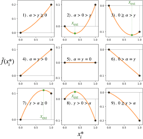
Figure 5: All possible $\tilde{f}(x_{i}^{*})$ depending on $\alpha$ and $\gamma$. The orange lines show $\tilde{f}(x_{i}^{*})$ for the horizontal axis of $x_{i}^{*}$. The black dots are the values in $x_{i}^{*}=0$ and $1$. The green dots show the extreme value in $x_{{\rm ext}}:=\gamma/\{2(\gamma-\alpha)\}$; $0<x_{{\rm ext}}<1/2$ in the cases of 2) and 8), while $1/2<x_{{\rm ext}}<1$ in the cases of 3) and 7).

Case 5).

In this case, $\tilde{f}(x_{i}^{*})=0$ always holds. Thus, all the interior points of the strategy space are the Nash equilibrium, i.e., $\bm{x}^{*}\in{\rm int}\ (\Delta^{m-1})$.

Case 1) 3) 4) 6) 7) 9).

In these cases, $\tilde{f}(x_{i}^{*})=C$ has no multiple solutions in $0<x_{i}^{*}<1/2$. Thus, the interior Nash equilibrium is only $\bm{x}^{*}\in\{\bm{1}/m\}=:\mathcal{N}_{\rm U}(m)$ (U: Uniform-choice equilibrium).

Case 2) 8).

In these cases, $\tilde{f}(x_{i}^{*})$ is parabolic and takes its extreme value at $x_{i}^{*}=\gamma/\{2(\gamma-\alpha)\}=:x_{{\rm ext}}$, which is in the region of $0<x_{{\rm ext}}<1/2$. Thus, for some $C$, $\tilde{f}(x_{i}^{*})=C$ has double roots $x_{i}^{*}=x_{+},x_{-}$, described as

$$x_{+}=x_{{\rm ext}}+\delta,\ x_{-}=x_{{\rm ext}}-\delta,$$ (42)

with $0<\delta<x_{{\rm ext}}$. Here, a condition for a strategy which composes of $k$-pieces of $x_{+}$ and $(m-k)$-pieces of $x_{-}$ for $k\in\{1,\cdots,m-1\}$, i.e.,

$$\bm{x}_{{\rm DR};k}:=(\underbrace{x_{+},\cdots,x_{+}}_{k},\underbrace{x_{-},\cdots,x_{-}}_{m-k})$$ (43)

to be the Nash equilibrium is

$$kx_{+}+(m-k)x_{-}=1 \Leftrightarrow mx_{{\rm ext}}-(m-2k)\delta=1$$ (44)

$$\Leftrightarrow\delta=\frac{mx_{{\rm ext}}-1}{m-2k}.$$ (45)

Since $0<\delta\leq x_{{\rm ext}}$ should be satisfied, we solve

$$0<\frac{mx_{{\rm ext}}-1}{m-2k}<x_{{\rm ext}}\Leftrightarrow\begin{cases}\displaystyle k<\frac{1}{2x_{{\rm ext}}}&\displaystyle\left(x_{{\rm ext}}>\frac{1}{m}\right)\\ \displaystyle k>\frac{1}{2x_{{\rm ext}}}&\displaystyle\left(x_{{\rm ext}}<\frac{1}{m}\right)\\ \end{cases}.$$ (46)

In conclusion, the interior Nash equilibria include

$$\bm{x}^{*} \in\begin{cases}\{\sigma(\bm{x}_{{\rm DR};k})|\sigma\in S_{m},k=1,\cdots,\lfloor 1/(2x_{{\rm ext}})\rfloor\}&(x_{{\rm ext}}>1/m)\\ \{\sigma(\bm{x}_{{\rm DR};k})|\sigma\in S_{m},k=\lceil 1/(2x_{{\rm ext}})\rceil,\cdots,m-1\}&(x_{{\rm ext}}<1/m)\\ \end{cases}$$ (47)

$$=:\mathcal{N}_{\rm DR}(m),$$ (48)

(DR: Double Roots equilibria). Here, $\sigma$ is a permutation function in the $m$-dimensional symmetric group $S_{m}$. Since the uniform-choice equilibrium is also included, all the interior Nash equilibria are given by $\mathcal{N}_{\rm U}(m)\cup\mathcal{N}_{\rm DR}(m)$. ∎

A.4 Proof of Lemma 6

Proof.

In the interior of the strategy space, the condition for $\bm{x}^{*}$ is, with some $C$ for all $i\in\{1,\cdots,m\}$,

$$\begin{cases}x_{i}^{*}>0&\Rightarrow\tilde{f}(x_{i}^{*})=C\\ x_{i}^{*}=0&\Rightarrow\tilde{f}(x_{i}^{*})\leq C\\ \end{cases}.$$ (49)

This is equivalent to, with some $C\geq 0(\Leftrightarrow\tilde{f}(0)\leq C)$ for all $i$ such that $x_{i}^{*}>0$,

$$\tilde{f}(x_{i}^{*})=C.$$ (50)

In the following, we consider this condition under the classification of $\alpha$ and $\gamma$ (see Fig. 5 again).

Case 5).

In this case, $\tilde{f}(x_{i}^{*})=0$ always holds. Thus, all the boundary points of the strategy space are the Nash equilibrium, i.e., $\bm{x}^{*}\in\partial\Delta^{m-1}$.

Case 3) 6) 9).

In these cases, $\tilde{f}(x_{i}^{*})<0=\tilde{f}(0)$ always holds for $0<x_{i}^{*}\leq 1$. Thus, there is no boundary Nash equilibrium.

Case 1) 4) 7).

In these cases, $\tilde{f}(x_{i}^{*})\geq 0=\tilde{f}(0)$ is positive for all $0\leq x_{i}^{*}\leq 1$. In other words, $\tilde{f}(1)\geq\tilde{f}(0)$ holds, meaning that the boundary Nash equilibria include $\{\bm{e}_{1},\cdots,\bm{e}_{m}\}=:\mathcal{N}_{\rm P}(m)$ (P: Pure-strategy equilibria). Furthermore, for $2\leq m^{\prime}\leq m-1$, $\tilde{f}(1/m^{\prime})\geq\tilde{f}(0)$ also holds so that the boundary Nash equilibria also include $\mathrm{Proj}^{-1}(\mathcal{N}_{\rm U}(m^{\prime}))$ for all $m^{\prime}\in\{2,\cdots,m-1\}=:A$. Here, $\mathrm{Proj}^{-1}$ shows the inverse projection from $m^{\prime}<m$- to $m$-dimensional space with arbitrary permutations. Thus, the Nash equilibria are given by

$$\mathcal{N}_{\rm P}(m)\cup\left(\bigcup_{m^{\prime}\in A}\mathrm{Proj}^{-1}(\mathcal{N}_{\rm U}(m^{\prime}))\right).$$ (51)

case 2).

In this case, $\tilde{f}(x_{i}^{*})\geq 0=\tilde{f}(0)$ holds for $x_{{\rm ext}}\leq x_{i}^{*}\leq 1$. Thus, since $\tilde{f}(1)\geq\tilde{f}(0)$ holds, the Nash equilibria include $\mathcal{N}_{\rm P}(m)$. Furthermore, since $\tilde{f}(1/m^{\prime})\geq\tilde{f}(0)$ holds for $2\leq m^{\prime}\leq 1/x_{{\rm ext}}$, the Nash equilibria include $\mathrm{Proj}^{-1}(\mathcal{N}_{\rm U}(m^{\prime}))$ for all $m^{\prime}\in\{2,\cdots,\min(\lfloor 1/x_{{\rm ext}}\rfloor,m-1)\}=:A^{(-)}$. To summarize, the Nash equilibria are given by

$$\mathcal{N}_{\rm P}(m)\cup\left(\bigcup_{m^{\prime}\in A^{(-)}}\mathrm{Proj}^{-1}(\mathcal{N}_{\rm U}(m^{\prime}))\right).$$ (52)

Case 8).

In this case, $\tilde{f}(x_{i}^{*})\geq 0=\tilde{f}(0)$ holds for $0<x_{i}^{*}\leq x_{{\rm ext}}$. Thus, the Nash equilibria include $\mathrm{Proj}^{-1}(\mathcal{N}_{\rm DR}(m^{\prime}))$ for all $m^{\prime}\in A$. Furthermore, the Nash equilibria also include $\mathrm{Proj}^{-1}(\mathcal{N}_{\rm U}(m^{\prime}))$ for all $m^{\prime}\in\{\lceil 1/(2x_{{\rm ext}})\rceil,\cdots,m-1\}=:A^{(+)}$. To summarize, the Nash equilibria are given by $\mathcal{N}_{\rm U}(1/(2x_{{\rm ext}})\leq m^{\prime}\leq m-1)\cup\mathcal{N}_{\rm DR}(2\leq m^{\prime}\leq m-1)$.

$$\left(\bigcup_{m^{\prime}\in A^{(+)}}\mathrm{Proj}^{-1}(\mathcal{N}_{\rm U}(m^{\prime}))\right)\cup\left(\bigcup_{m^{\prime}\in A}\mathrm{Proj}^{-1}(\mathcal{N}_{\rm DR}(m^{\prime}))\right)$$ (53)

∎

A.5 Proof of Lemma 3

Proof. Two-action games give $\bm{x}=(x_{1},x_{2})$, so that $x_{2}=\bar{x}_{1}$ holds. Similar equations hold for Y and Z. First, Eq. (14) in the FTRL algorithm is calculated as

$$q_{1}(\bm{x}^{\dagger}) =\arg\max_{\bm{x}}\{\bm{x}^{\dagger}\cdot\bm{x}-h(\bm{x})\}$$

$$=\arg\max_{x_{1}}\{x_{1}^{\dagger}x_{1}+x_{2}^{\dagger}(1-x_{1})-h_{{\rm two}}(x_{1})\}$$

$$=\arg\max_{x_{1}}\{\underbrace{(x_{1}^{\dagger}-x_{2}^{\dagger})}_{=:\Delta x^{\dagger}}x_{1}-h_{{\rm two}}(x_{1})\}$$ (54)

Thus, $q_{1}(\bm{x}^{\dagger})$ is determined only by the single variable of $\Delta x^{\dagger}$, which dynamics are

$$\Delta\dot{x}^{\dagger} =\dot{x}_{1}^{\dagger}-\dot{x}_{2}^{\dagger}$$

$$=\frac{\partial u}{\partial x_{1}}-\frac{\partial u}{\partial x_{2}}$$

$$=f(y_{1},z_{1})-f(y_{2},z_{2})$$

$$=f(y_{1},z_{1})-f(1-y_{1},1-z_{1})$$

$$=(\alpha+\beta)y_{1}+(\alpha-\beta)z_{1}-\alpha=:f_{{\rm two}}(y_{1},z_{1}),$$ (55)

independent of $\gamma$.

We further assume $\bm{x}\in{\rm int}\ \Delta^{m-1}$, i.e., $0<x_{1}<1$. Then, the extreme condition in Eq. (54) is calculated as

$$h_{{\rm two}}^{\prime}(q_{1}(\bm{x}^{\dagger}))=\Delta x^{\dagger}\Leftrightarrow q_{1}(\bm{x}^{\dagger})=h_{{\rm two}}^{\prime-1}(\Delta x^{\dagger}).$$ (56)

By this equation, we obtain

$$\dot{x}_{1} =\frac{\partial u}{\partial x_{1}}\frac{\partial q_{1}}{\partial x_{1}^{\dagger}}+\frac{\partial u}{\partial x_{2}}\frac{\partial q_{1}}{\partial x_{2}^{\dagger}}$$

$$=\frac{\partial u}{\partial x_{1}}(h_{{\rm two}}^{\prime-1})^{\prime}(\Delta x^{\dagger})-\frac{\partial u}{\partial x_{2}}(h_{{\rm two}}^{\prime-1})^{\prime}(\Delta x^{\dagger})$$

$$=(f(y_{1},z_{1})-f(y_{2},z_{2}))(h_{{\rm two}}^{\prime-1})^{\prime}(\Delta x^{\dagger})$$

$$=f_{{\rm two}}(y_{1},z_{1})(h_{{\rm two}}^{\prime-1})^{\prime}(\Delta x^{\dagger}),$$ (57)

Let us calculate $(h_{{\rm two}}^{\prime-1})^{\prime}(\Delta x^{\dagger})$ as

$$h_{{\rm two}}(x_{1})=x_{1}\log x_{1}+(1-x_{1})\log(1-x_{1})$$

$$\Leftrightarrow h_{{\rm two}}^{\prime}(x_{1})=\log x_{1}-\log(1-x_{1})\ (=\Delta x^{\dagger})$$

$$\Leftrightarrow h_{{\rm two}}^{\prime-1}(\Delta x^{\dagger})=\frac{\exp(\Delta x^{\dagger})}{1+\exp(\Delta x^{\dagger})}\ (=x_{1})$$

$$\Leftrightarrow (h_{{\rm two}}^{\prime-1})^{\prime}(\Delta x^{\dagger})=\frac{\exp(\Delta x^{\dagger})}{1+\exp(\Delta x^{\dagger})}\frac{1}{1+\exp(\Delta x^{\dagger})}=x_{1}(1-x_{1}),$$ (58)

for the entropic regularizer $h(\bm{x})=\bm{x}\cdot\log\bm{x}$ and

$$h_{{\rm two}}(x_{1})=\frac{x_{1}^{2}+(1-x_{1})^{2}}{2}$$

$$\Leftrightarrow h_{{\rm two}}^{\prime}(x_{1})=2x_{1}-1\ (=\Delta x^{\dagger})$$

$$\Leftrightarrow h_{{\rm two}}^{\prime-1}(\Delta x^{\dagger})=\frac{\Delta x^{\dagger}+1}{2}\ (=x_{1})$$

$$\Leftrightarrow (h_{{\rm two}}^{\prime-1})^{\prime}(\Delta x^{\dagger})=\frac{1}{2},$$ (59)

for the Euclidean regularizer $h(\bm{x})=\|\bm{x}\|^{2}/2$. To summarize, we denote $(h_{{\rm two}}^{\prime-1})^{\prime}(\Delta x^{\dagger})$ by

$$w(x_{1}) :=\begin{cases}x_{1}(1-x_{1})&(h(\bm{x})=\bm{x}\cdot\log\bm{x})\\ 1/2&(h(\bm{x})=\|\bm{x}\|^{2}/2)\\ \end{cases}.$$ (60)

∎

A.6 Proof of Theorem 2

Proof.

In two-action games, we obtain

$$V(\bm{x},\bm{y},\bm{z})=x_{1}y_{1}z_{1}+(1-x_{1})(1-y_{1})(1-z_{1}).$$ (61)

We now define the cyclic sum $\Sigma_{\rm cyc}\$ as

$$\Sigma_{\rm cyc}\ \mathcal{F}(\bm{x},\bm{y},\bm{z}):=\mathcal{F}(\bm{x},\bm{y},\bm{z})+\mathcal{F}(\bm{y},\bm{z},\bm{x})+\mathcal{F}(\bm{z},\bm{x},\bm{y}),$$ (62)

for arbitrary function $\mathcal{F}$. Using this $\Sigma_{\rm cyc}\$, $V$ is calculated as

$$\dot{V} =\Sigma_{\rm cyc}\ \dot{x}_{1}y_{1}z_{1}-\dot{x}_{1}(1-y_{1})(1-z_{1})$$

$$=\Sigma_{\rm cyc}\ w(x_{1})\{\alpha(y_{1}+z_{1}-1)+\beta(y_{1}-z_{1})\}(y_{1}+z_{1}-1)$$

$$=\alpha\Sigma_{\rm cyc}\ w(x_{1})(y_{1}+z_{1}-1)^{2}+\beta w(x_{1})(y_{1}-z_{1})(y_{1}+z_{1}-1)$$

$$=\alpha\Sigma_{\rm cyc}\ w(x_{1})(y_{1}+z_{1}-1)^{2},$$ (63)

Here, because $w(x_{1})>0$ always holds, ${\rm sign}(\dot{V})={\rm sign}(\alpha)$ is proved. In the last line of this equation, we used

$$\Sigma_{\rm cyc}\ w(x_{1})(y_{1}-z_{1})(y_{1}+z_{1}-1)$$

$$=\Sigma_{\rm cyc}\ x_{1}(1-x_{1})(y_{1}-z_{1})(y_{1}+z_{1}-1)$$

$$=-\underbrace{\Sigma_{\rm cyc}\ x_{1}(y_{1}-z_{1})}_{=0}-\underbrace{\Sigma_{\rm cyc}\ x_{1}^{2}(y_{1}^{2}-z_{1}^{2})}_{=0}+\underbrace{\Sigma_{\rm cyc}\ (x_{1}y_{1}^{2}-z_{1}x_{1}^{2})}_{=0}+\underbrace{\Sigma_{\rm cyc}\ (x_{1}^{2}y_{1}-z_{1}^{2}x_{1})}_{=0}$$

$$=0,$$ (64)

for the entropic regularizer $w(x_{1})=x_{1}(1-x_{1})$ and

$$\Sigma_{\rm cyc}\ w(x_{1})(y_{1}-z_{1})(y_{1}+z_{1}-1)$$

$$=\frac{1}{2}\Sigma_{\rm cyc}\ (y_{1}-z_{1})(y_{1}+z_{1}-1)$$

$$=\frac{1}{2}\underbrace{\Sigma_{\rm cyc}\ (y_{1}^{2}-z_{1}^{2})}_{=0}-\frac{1}{2}\underbrace{\Sigma_{\rm cyc}\ (y_{1}-z_{1})}_{=0}$$

$$=0,$$ (65)

for the Euclidean regularizer $w(x_{1})=1/2$. ∎

A.7 Proof of Theorem 3

Proof.

First, we can derive

$$\dot{G} =\Sigma_{\rm cyc}\ \Sigma_{i}\ \frac{\partial u}{\partial x_{i}}(x_{i}-x_{i}^{*})$$

$$=\Sigma_{\rm cyc}\ \Sigma_{i}\ f(y_{i},z_{i})(x_{i}-x_{i}^{*})$$

$$=\Sigma_{\rm cyc}\ f_{{\rm two}}(y_{1},z_{1})(x_{1}-x_{1}^{*})$$

$$=\Sigma_{\rm cyc}\ \{\alpha(y_{1}+z_{1}-1)+\beta(y_{1}-z_{1})\}(x_{1}-x_{1}^{*})$$

$$=\alpha\Sigma_{\rm cyc}\ (y_{1}+z_{1}-1)(x_{1}-x_{1}^{*})$$

$$=2\alpha\left\{(x_{1}y_{1}+y_{1}z_{1}+z_{1}x_{1})-(x_{1}+y_{1}+z_{1})+\frac{3}{4}\right\}$$

$$=2\alpha V.$$ (66)

Here, in the fifth equal sign, the term of $\beta$ disappears because

$$\Sigma_{\rm cyc}\ (y_{1}-z_{1})(x_{1}-x_{1}^{*})$$

$$=\Sigma_{\rm cyc}\ (y_{1}-z_{1})\left(x_{1}-\frac{1}{2}\right)$$

$$=\underbrace{\Sigma_{\rm cyc}\ x_{1}(y_{1}-z_{1})}_{=0}-\frac{1}{2}\underbrace{\Sigma_{\rm cyc}\ (y_{1}-z_{1})}_{=0}$$

$$=0.$$ (67)

The sixth equal sign holds because

$$V =\Sigma_{i}\ x_{i}y_{i}z_{i}-\frac{1}{m^{2}}$$

$$=x_{1}y_{1}z_{1}+(1-x_{1})(1-y_{1})(1-z_{1})-\frac{1}{4}$$

$$=(x_{1}y_{1}+y_{1}z_{1}+z_{1}x_{1})-(x_{1}+y_{1}+z_{1})+\frac{3}{4}.$$ (68)

∎

A.8 Proof of Theorem 4

Proof.

$$\dot{V} =\Sigma_{\rm cyc}\ \Sigma_{i}\ \dot{x}_{i}y_{i}z_{i}$$

$$=\Sigma_{\rm cyc}\ \Sigma_{i}\ x_{i}y_{i}z_{i}(f(y_{i},z_{i})-\Sigma_{i}\ x_{i}f(y_{i},z_{i}))$$

$$=\alpha\Sigma_{\rm cyc}\ \Sigma_{i}\ x_{i}y_{i}z_{i}(y_{i}z_{i}-\Sigma_{i}\ x_{i}y_{i}z_{i})+\frac{\beta}{2}\Sigma_{\rm cyc}\ \Sigma_{i}\ x_{i}y_{i}z_{i}\{(y_{i}-z_{i})-\Sigma_{i}\ x_{i}(y_{i}-z_{i})\}$$

$$=\alpha\Sigma_{\rm cyc}\ \Sigma_{i}\ x_{i}y_{i}z_{i}(y_{i}z_{i}-\Sigma_{i}\ x_{i}y_{i}z_{i})$$

$$=\alpha\Sigma_{\rm cyc}\ \{\Sigma_{i}\ x_{i}(y_{i}z_{i})^{2}-(\Sigma_{i}\ x_{i}y_{i}z_{i})^{2}\}$$

$$=\alpha\Sigma_{\rm cyc}\ {\rm Var}[y_{i}z_{i}]_{x_{i}}.$$ (69)

Here, ${\rm Var}[y_{i}z_{i}]_{x_{i}}$ shows the variance of $y_{i}z_{i}$ based on the distribution of $x_{i}$ for $i$. In the fourth equal sign, we used

$$\Sigma_{\rm cyc}\ \Sigma_{i}\ x_{i}y_{i}z_{i}\{(y_{i}-z_{i})-\Sigma_{i}\ x_{i}(y_{i}-z_{i})\}$$

$$=\Sigma_{i}\ x_{i}y_{i}z_{i}\{\underbrace{\Sigma_{\rm cyc}\ (y_{i}-z_{i})}_{=0}-\Sigma_{i}\ \underbrace{\Sigma_{\rm cyc}\ x_{i}(y_{i}-z_{i})}_{=0}\}$$

$$=0.$$ (70)

From the definition of variance, ${\rm Var}[y_{i}z_{i}]_{x_{i}}=0$ holds if and only if $y_{i}z_{i}$ takes a constant value $C_{X}$ for all $i$. Thus, the condition for $\Sigma_{\rm cyc}\ {\rm Var}[y_{i}z_{i}]_{x_{i}}=0$ is

$$\begin{cases}y_{i}z_{i}=C_{X}\\ z_{i}x_{i}=C_{Y}\\ x_{i}y_{i}=C_{Z}\\ \end{cases},$$ (71)

for some constants $C_{X}$, $C_{Y}$, and $C_{Z}$. In the same way as the proof of Lem. 4, the condition is equivalent to $\bm{x}=\bm{y}=\bm{z}=\bm{1}/m$, meaning the uniform-choice equilibrium. ∎

References

- Abe et al. [2022] Kenshi Abe, Mitsuki Sakamoto, and Atsushi Iwasaki. Mutation-driven follow the regularized leader for last-iterate convergence in zero-sum games. In UAI, pages 1–10, 2022.
- Abe et al. [2023] Kenshi Abe, Kaito Ariu, Mitsuki Sakamoto, Kentaro Toyoshima, and Atsushi Iwasaki. Last-iterate convergence with full and noisy feedback in two-player zero-sum games. In AISTATS, pages 7999–8028, 2023.
- Akiyama and Kaneko [2000] Eizo Akiyama and Kunihiko Kaneko. Dynamical systems game theory and dynamics of games. Physica D: Nonlinear Phenomena, 147(3-4):221–258, 2000.
- Anagnostides et al. [2022] Ioannis Anagnostides, Ioannis Panageas, Gabriele Farina, and Tuomas Sandholm. On last-iterate convergence beyond zero-sum games. In ICML, pages 536–581, 2022.
- Bailey and Piliouras [2019] James P Bailey and Georgios Piliouras. Multi-agent learning in network zero-sum games is a hamiltonian system. In AAMAS, pages 233–241, 2019.
- Bloembergen et al. [2015] Daan Bloembergen, Karl Tuyls, Daniel Hennes, and Michael Kaisers. Evolutionary dynamics of multi-agent learning: A survey. Journal of Artificial Intelligence Research, 53:659–697, 2015.
- Börgers and Sarin [1997] Tilman Börgers and Rajiv Sarin. Learning through reinforcement and replicator dynamics. Journal of Economic Theory, 77(1):1–14, 1997.
- Bowling [2000] Michael Bowling. Convergence problems of general-sum multiagent reinforcement learning. In ICML, pages 89–94, 2000.
- Brown [1951] George W Brown. Iterative solution of games by fictitious play. Act. Anal. Prod Allocation, 13(1):374, 1951.
- Brown and Sandholm [2019] Noam Brown and Tuomas Sandholm. Superhuman ai for multiplayer poker. Science, 365(6456):885–890, 2019.
- Chen and Deng [2006] Xi Chen and Xiaotie Deng. Settling the complexity of two-player nash equilibrium. In FOCS, volume 6, pages 261–272, 2006.
- Daskalakis and Panageas [2019] Constantinos Daskalakis and Ioannis Panageas. Last-iterate convergence: Zero-sum games and constrained min-max optimization. In ITCS, pages 27:1–27:18, 2019.
- Daskalakis and Papadimitriou [2005] Constantinos Daskalakis and Christos H Papadimitriou. Three-player games are hard. In Electronic colloquium on computational complexity, volume 139, pages 81–87. Citeseer, 2005.
- Daskalakis et al. [2009] Constantinos Daskalakis, Paul W Goldberg, and Christos H Papadimitriou. The complexity of computing a nash equilibrium. Communications of the ACM, 52(2):89–97, 2009.
- Dieckmann and Law [1996] Ulf Dieckmann and Richard Law. The dynamical theory of coevolution: a derivation from stochastic ecological processes. Journal of mathematical biology, 34:579–612, 1996.
- Friedman [1991] Daniel Friedman. Evolutionary games in economics. Econometrica: Journal of the Econometric Society, pages 637–666, 1991.
- Fudenberg and Levine [1998] Drew Fudenberg and David K Levine. The theory of learning in games, volume 2. MIT press, 1998.
- Fujimoto and Kaneko [2019] Yuma Fujimoto and Kunihiko Kaneko. Emergence of exploitation as symmetry breaking in iterated prisoner’s dilemma. Physical Review Research, 1(3):033077, 2019.
- Fujimoto and Kaneko [2021] Yuma Fujimoto and Kunihiko Kaneko. Exploitation by asymmetry of information reference in coevolutionary learning in prisoner’s dilemma game. Journal of Physics: Complexity, 2(4):045007, 2021.
- Fujimoto et al. [2023] Yuma Fujimoto, Kaito Ariu, and Kenshi Abe. Learning in multi-memory games triggers complex dynamics diverging from nash equilibrium. In IJCAI, 2023.
- Fujimoto et al. [2024] Yuma Fujimoto, Kaito Ariu, and Kenshi Abe. Memory asymmetry creates heteroclinic orbits to nash equilibrium in learning in zero-sum games. In AAAI, 2024.
- Gaunersdorfer and Hofbauer [1995] Andrea Gaunersdorfer and Josef Hofbauer. Fictitious play, shapley polygons, and the replicator equation. Games and Economic Behavior, 11(2):279–303, 1995.
- Grant [2023] William C Grant. Correlated equilibrium and evolutionary stability in 3-player rock-paper-scissors. Games, 14(3):45, 2023.
- Hofbauer and Sigmund [1990] Josef Hofbauer and Karl Sigmund. Adaptive dynamics and evolutionary stability. Applied Mathematics Letters, 3(4):75–79, 1990.
- Hofbauer et al. [1998] Josef Hofbauer, Karl Sigmund, et al. Evolutionary games and population dynamics. Cambridge university press, 1998.
- Jordan [1993] James S Jordan. Three problems in learning mixed-strategy nash equilibria. Games and Economic Behavior, 5(3):368–386, 1993.
- Li et al. [2020] Junjie Li, Sotetsu Koyamada, Qiwei Ye, Guoqing Liu, Chao Wang, Ruihan Yang, Li Zhao, Tao Qin, Tie-Yan Liu, and Hsiao-Wuen Hon. Suphx: Mastering mahjong with deep reinforcement learning. arXiv preprint arXiv:2003.13590, 2020.
- McCabe et al. [2000] Kevin A McCabe, Arijit Mukherji, and David E Runkle. An experimental study of information and mixed-strategy play in the three-person matching-pennies game. Economic Theory, 15:421–462, 2000.
- Mealing and Shapiro [2015] Richard Mealing and Jonathan L Shapiro. Convergence of strategies in simple co-adapting games. In FOGA, pages 176–190, 2015.
- Mertikopoulos and Sandholm [2016] Panayotis Mertikopoulos and William H Sandholm. Learning in games via reinforcement and regularization. Mathematics of Operations Research, 41(4):1297–1324, 2016.
- Mertikopoulos et al. [2018] Panayotis Mertikopoulos, Christos Papadimitriou, and Georgios Piliouras. Cycles in adversarial regularized learning. In SODA, pages 2703–2717, 2018.
- Mertikopoulos et al. [2019] Panayotis Mertikopoulos, Bruno Lecouat, Houssam Zenati, Chuan-Sheng Foo, Vijay Chandrasekhar, and Georgios Piliouras. Optimistic mirror descent in saddle-point problems: Going the extra(-gradient) mile. In ICLR, 2019.
- Murase and Baek [2018] Yohsuke Murase and Seung Ki Baek. Seven rules to avoid the tragedy of the commons. Journal of theoretical biology, 449:94–102, 2018.
- Nash Jr [1950] John F Nash Jr. Equilibrium points in n-person games. Proceedings of the National Academy of Sciences, 36(1):48–49, 1950.
- Paquette et al. [2019] Philip Paquette, Yuchen Lu, Seton Steven Bocco, Max Smith, Satya O-G, Jonathan K Kummerfeld, Joelle Pineau, Satinder Singh, and Aaron C Courville. No-press diplomacy: Modeling multi-agent gameplay. In NeurIPS, volume 32, 2019.
- Piliouras et al. [2014] Georgios Piliouras, Carlos Nieto-Granda, Henrik I Christensen, and Jeff S Shamma. Persistent patterns: Multi-agent learning beyond equilibrium and utility. In AAMAS, pages 181–188, 2014.
- Sato et al. [2002] Yuzuru Sato, Eizo Akiyama, and J Doyne Farmer. Chaos in learning a simple two-person game. Proceedings of the National Academy of Sciences, 99(7):4748–4751, 2002.
- Sato et al. [2005] Yuzuru Sato, Eizo Akiyama, and James P Crutchfield. Stability and diversity in collective adaptation. Physica D: Nonlinear Phenomena, 210(1-2):21–57, 2005.
- Shalev-Shwartz and Singer [2006] Shai Shalev-Shwartz and Yoram Singer. Convex repeated games and fenchel duality. In NeurIPS, volume 19, 2006.
- Shamma and Arslan [2005] Jeff S Shamma and Gürdal Arslan. Dynamic fictitious play, dynamic gradient play, and distributed convergence to nash equilibria. IEEE Transactions on Automatic Control, 50(3):312–327, 2005.
- Singh et al. [2000] Satinder Singh, Michael J Kearns, and Yishay Mansour. Nash convergence of gradient dynamics in general-sum games. In UAI, pages 541–548, 2000.
- Szafron et al. [2013] Duane Szafron, Richard G Gibson, and Nathan R Sturtevant. A parameterized family of equilibrium profiles for three-player kuhn poker. In AAMAS, volume 13, pages 247–254, 2013.
- Taylor and Jonker [1978] Peter D Taylor and Leo B Jonker. Evolutionary stable strategies and game dynamics. Mathematical biosciences, 40(1-2):145–156, 1978.
- Tuyls and Nowé [2005] Karl Tuyls and Ann Nowé. Evolutionary game theory and multi-agent reinforcement learning. The Knowledge Engineering Review, 20(1):63–90, 2005.
- Tuyls et al. [2006] Karl Tuyls, Pieter Jan’T Hoen, and Bram Vanschoenwinkel. An evolutionary dynamical analysis of multi-agent learning in iterated games. In AAMAS, volume 12, pages 115–153. Springer, 2006.
- Ueda [2023] Masahiko Ueda. Memory-two strategies forming symmetric mutual reinforcement learning equilibrium in repeated prisoners’ dilemma game. Applied Mathematics and Computation, 444:127819, 2023.
- Usui and Ueda [2021] Yuki Usui and Masahiko Ueda. Symmetric equilibrium of multi-agent reinforcement learning in repeated prisoner’s dilemma. Applied Mathematics and Computation, 409:126370, 2021.
- Zinkevich [2003] Martin Zinkevich. Online convex programming and generalized infinitesimal gradient ascent. In ICML, pages 928–936, 2003.