Kadanoff-Baym equations for interacting systems with dissipative Lindbladian dynamics

Abstract

The extraordinary quantum properties of nonequilibrium systems governed by dissipative dynamics have become a focal point in contemporary scientific inquiry. The Nonequilibrium Green’s Functions (NEGF) theory provides a versatile method for addressing driven non-dissipative systems, utilizing the powerful diagrammatic technique to incorporate correlation effects. We here present a second-quantization approach to the dissipative NEGF theory, reformulating Keldysh ideas to accommodate Lindbladian dynamics and extending the Kadanoff-Baym equations accordingly. Generalizing diagrammatic perturbation theory for many-body Lindblad operators, the formalism enables correlated and dissipative real-time simulations for the exploration of transient and steady-state changes in the electronic, transport, and optical properties of materials.

Nonequilibrium systems governed by dissipative dynamics have broken into modern science owing to their remarkable quantum properties. Optical cavities of atoms Ritsch et al. (2013); Baumann et al. (2010), molecules Flick et al. (2017); Mandal et al. (2023) and solid state systems Hübener et al. (2021); Schlawin et al. (2022) offer an ideal platform to exploit the interplay between coherence and dissipation Verstraete et al. (2009). Special attention has thus far been dedicated to stationary states – in particular the study of non-equilibrium fixed points and critical exponents Sieberer et al. (2013); Kulkarni et al. (2013), phase transitions Dalla Torre et al. (2010); Raftery et al. (2014), entanglement Krauter et al. (2011); Kastoryano et al. (2011), and topology Bergholtz et al. (2021) – as well as Floquet states Sato et al. (2020); Mori (2023).

The transient dynamics of dissipative systems subjected to ultrafast driving fields remains poorly explored. In fact, the concomitant action of external fields, correlation and dissipation calls for innovative many-body frameworks. The Lindblad equation Lindblad (1976); Breuer and Petruccione (2007) serves as a solid ground to incorporate the aforementioned physics, preserving the trace and positivity of the many-body density matrix $\hat{\rho}$. However, its brute force numerical solution scales exponentially with the system size. Nonequilibrium Green’s functions (NEGF) theory Stefanucci and van Leeuwen (2013); Kamenev (2011); Haug and Jauho (2008) has proven to be a versatile tool to deal with driven systems; it leverages the powerful diagrammatic technique to account for correlation effects, thus reducing from exponential to power-law the numerical scaling. The inclusion of Lindblad dissipation in NEGF has been accomplished by Sieberer et al. in the so called field theory approach Sieberer et al. (2016); Fogedby (2022); Thompson and Kamenev (2023); Sieberer et al. (2023), which is based on the path integral technique and Schwinger-Keldysh action Altland and Simons (2010). Alternatively, NEGF can be formulated in the second-quantization approach Rammer (2007); Stefanucci and van Leeuwen (2013); Balzer and Bonitz (2013); Stefanucci et al. (2023), where concepts like the Martin-Schwinger hierarchy Martin and Schwinger (1959), Kadanoff-Baym equations kb- ; Danielewicz (1984), conserving approximations Baym and Kadanoff (1961); Baym (1962) and Bethe-Salpeter equation Strinati (1986); Sander et al. (2015) are employed to develop many-body schemes for the simulation of carrier Steinhoff et al. (2016); Molina-Sánchez et al. (2017); Perfetto et al. (2022) and phonon Tong and Bernardi (2021); Caruso (2021); Caruso and Novko (2022) dynamics, dephasing and thermalization Perfetto and Stefanucci (2023), transient photoabsorbtion Attaccalite et al. (2011); Jiang et al. (2021); Perfetto et al. (2015); Tuovinen et al. (2020), photoemission Freericks et al. (2009); Perfetto et al. (2016) and Raman Galperin et al. (2009); Werner et al. (2023) spectroscopy, photoexcitations and quenches in Mott and excitonic insulators Aoki et al. (2014); Eckstein et al. (2009); Murakami et al. (2017); Schüler et al. (2020), or time-dependent quantum transport Meir and Wingreen (1992); Jauho et al. (1994); Galperin et al. (2007); Myöhänen et al. (2008, 2009); Puig von Friesen et al. (2010); Schwarz et al. (2016). The question of how the second-quantization approach – and related concepts – should be extended to encompass dissipation remains to be elucidated.

In this work we offer a second-quantization perspective on the dissipative NEGF theory. We reformulate the original Keldysh idea to accommodate Lindbladian time-evolutions, and extend the Kadanoff-Baym equations accordingly. We also show how to generalize the diagrammatic perturbation theory for many-body Lindblad operators. The resulting formalism paves the way for real-time simulations of the correlated and dissipative dynamics of materials.

Keldysh-Lindblad formalism.– For systems with dissipative Lindbladian dynamics the average value of any, generally time-dependent, operator $\hat{O}(t)$ at time $t$ is expressed as $O(t)={\rm Tr}\big{[}\hat{\rho}(t)\hat{O}(t)\big{]}$, where the many-body density matrix satisfies the Lindblad equation (henceforth sum over repeated indices is implicit)

$$\frac{d\hat{\rho}}{dt} =-i[\hat{H},\hat{\rho}]_{-}+2\hat{L}_{\gamma}\hat{\rho}\hat{L}^{\dagger}_{\gamma}-\hat{L}^{\dagger}_{\gamma}\hat{L}_{\gamma}\hat{\rho}-\hat{\rho}\hat{L}^{\dagger}_{\gamma}\hat{L}_{\gamma}.$$ (1)

Here, $\hat{H}$ is the self-adjoint Hamiltonian of the system and $\hat{L}_{\gamma}$ are the Lindblad operators. Equation (1) can equivalently be cast in the form of an integral equation. Let $\hat{H}_{o}(t)=\hat{H}(t)-i\hat{L}^{\dagger}_{\gamma}(t)\hat{L}_{\gamma}(t)$ be the “open system” Hamiltonian and define the nonunitary evolution operator $\hat{U}_{o}(t,t^{\prime})=Te^{-i\int_{t^{\prime}}^{t}d\bar{t}\hat{H}_{o}(\bar{t})}$ for $t>t^{\prime}$ and $\hat{U}_{o}(t,t^{\prime})=\overline{T}e^{-i\int_{t^{\prime}}^{t}d\bar{t}\hat{H}^{\dagger}_{o}(\bar{t})}$ for $t<t^{\prime}$, where $T$ and $\overline{T}$ are the time and anti-time ordering operators, respectively. Then $\hat{\rho}(t)=\hat{U}_{o}(t,0)\hat{\rho}(0)\hat{U}_{o}(0,t)+2\int_{0}^{t}dt_{1}\hat{U}_{o}(t,t_{1})\hat{L}_{\gamma_{1}}(t_{1})\hat{\rho}(t_{1})\hat{L}^{\dagger}_{\gamma_{1}}(t_{1})\hat{U}_{o}(t_{1},t)$ solves Eq. (1), as it can easily be verified by direct differentiation. Iterating the integral equation and using the cyclic property of the trace, the time-dependent average $O(t)$ reads

$$O(t) ={\rm Tr}\Big{[}\hat{\rho}(0)\sum_{k=0}^{\infty}2^{k}\int_{0}^{t}dt_{1}..\int_{0}^{t_{k-1}}dt_{k}\hat{U}_{o}(0,t_{k})L^{\dagger}_{\gamma_{k}}(t_{k})\ldots$$

$$\times\hat{U}_{o}(t_{2},t_{1})\hat{L}^{\dagger}_{\gamma_{1}}(t_{1})\hat{U}_{o}(t_{1},t)\hat{O}(t)\hat{U}_{o}(t,t_{1})\hat{L}_{\gamma_{1}}(t_{1})\hat{U}_{o}(t_{1},t_{2})$$

$$\times\ldots L_{\gamma_{k}}(t_{k})\hat{U}_{o}(t_{k},0)\Big{]}.$$ (2)

This result can be written in a more useful form if we introduce the oriented Keldysh contour $C=C_{-}\cup C_{+}=(0,t)\cup(t,0)$. Let $z^{\prime}\in C$ denote a contour-time and write $z^{\prime}=t^{\prime}_{\pm}$ if $z^{\prime}\in C_{\pm}$. We also define the functions $\theta_{\pm}(z^{\prime})=1$ if $z^{\prime}\in C_{\pm}$ and zero otherwise, and $s(z^{\prime})=\theta_{-}(z^{\prime})-\theta_{+}(z^{\prime})$. Then

$$\hat{U}_{o}(t_{i},t_{j})=\mbox{$\mathcal{T}$}\Big{\{}e^{-i\int_{t_{j\mp}}^{t_{i\mp}}d\bar{z}\big{[}\hat{H}(\bar{z})-is(\bar{z})\hat{L}^{\dagger}_{\gamma}(\bar{z})\hat{L}_{\gamma}(\bar{z})\big{]}}\Big{\}},\quad t_{i}\gtrless t_{j},$$ (3)

where $\mathcal{T}$ is the contour ordering operator. If we set the times of all operators $\hat{L}^{\dagger}$ on the $C_{+}$ branch and the times of all operators $\hat{L}$ on the $C_{-}$ branch then the string of operators in Eq. (2) is contour ordered. Therefore, taking into account that under the $\mathcal{T}$-sign the bosonic (fermionic) operators (anti)commute, we can extend all integration limits to $t$ and divide by $k!$. The re-ordering does not generate minus signs in the case of fermionic Lindblad operators since the number of interchanges is always even. In this way the series is transformed into the Taylor expansion of an exponential, and the time-dependent average simplifies to

$$O(t)={\rm Tr}\Big{[}\hat{\rho}(0)\mbox{$\mathcal{T}$}\Big{\{}e^{-i\int_{C}d\bar{z}\hat{H}(\bar{z},\bar{\text{\reflectbox{$z$}}})}\hat{O}(z)\Big{\}}\Big{]},$$ (4)

where

$$\hat{H}(\bar{z},\bar{\text{\reflectbox{$z$}}})=\hat{H}(\bar{z})-is(\bar{z})\hat{L}^{\dagger}_{\gamma}(\bar{z})\hat{L}_{\gamma}(\bar{z})+2i\theta_{-}(\bar{z})\hat{L}^{\dagger}_{\gamma}(\bar{\text{\reflectbox{$z$}}})\hat{L}_{\gamma}(\bar{z}),$$ (5)

and $\bar{\text{\reflectbox{$z$}}}=\bar{t}_{\mp}$ if $\bar{z}=\bar{t}_{\pm}$. Notice that under integration the last term in Eq. (5) can alternatively be written as $-2i\theta_{+}(\bar{z})\hat{L}^{\dagger}_{\gamma}(\bar{z})\hat{L}_{\gamma}(\bar{\text{\reflectbox{$z$}}})$ since $\int_{C}d\bar{z}F(\bar{z},\bar{\text{\reflectbox{$z$}}})=-\int_{C}d\bar{z}F(\bar{\text{\reflectbox{$z$}}},\bar{z})$ for any function $F$, and $\theta_{\pm}(\bar{z})=\theta_{\mp}(\bar{\text{\reflectbox{$z$}}})$. We also observe that in Eq. (4) the contour $C$ can be extended to infinity, i.e., $C=(0,\infty)\cup(\infty,0)$, since $\hat{K}\equiv\mbox{$\mathcal{T}$}\Big{\{}e^{-i\int_{t_{-}}^{t_{+}}d\bar{z}\hat{H}(\bar{z},\bar{\text{\reflectbox{$z$}}})}\Big{\}}=1$ for all $t$ not . This also implies that the contour-time $z$ of $\hat{O}$ can be either $t_{+}$ or $t_{-}$.

In analogy with the theory of unitary evolutions we define the one-particle Keldysh-Lindblad NEGF according to

$$G_{ij}(z,z^{\prime})=\frac{1}{i}{\rm Tr}\Big{[}\hat{\rho}(0)\mbox{$\mathcal{T}$}\Big{\{}e^{-i\int_{C}d\bar{z}\hat{H}(\bar{z},\bar{\text{\reflectbox{$z$}}})}\hat{d}_{i}(z)\hat{d}^{\dagger}_{j}(z^{\prime})\Big{\}}\Big{]},$$ (6)

where the annihilation operators $\hat{d}_{i}$ are either bosonic or fermionic, in which case $[\hat{d}_{i},\hat{d}^{\dagger}_{j}]_{\mp}=\delta_{ij}$ (upper sign for bosons and lower sign for fermions). The contour argument of $\hat{d}$ and $\hat{d}^{\dagger}$ in Eq. (6) fixes the position of these operators along the contour, thus rendering unambiguous the action of $\mathcal{T}$. The identity $\hat{K}=1$ implies that the NEGF satisfies the Keldysh properties $G(t_{+},t^{\prime}_{\pm})=G(t_{-},t^{\prime}_{\pm})$ for $t>t^{\prime}$ and $G(t_{\pm},t^{\prime}_{+})=G(t_{\pm},t^{\prime}_{-})$ for $t<t^{\prime}$.

Using the rules for the derivative of a contour-ordered string of operators, see Ref. Stefanucci and van Leeuwen (2013), and introducing the shorthand notation $\left\langle\ldots\right\rangle\equiv{\rm Tr}\Big{[}\hat{\rho}(0)\mbox{$\mathcal{T}$}\Big{\{}e^{-i\int_{C}d\bar{z}\hat{H}(\bar{z},\bar{\text{\reflectbox{$z$}}})}\ldots\Big{\}}\Big{]}$, we find the important result

$$i\frac{d}{dz}G_{ij}(z,z^{\prime}) =\frac{1}{i}\left\langle[\hat{d}_{i}(z),\hat{H}(z)-is(z)\hat{L}^{\dagger}_{\gamma}(z)\hat{L}_{\gamma}(z)]_{-}\hat{d}^{\dagger}_{j}(z^{\prime})\right\rangle$$

$$- 2\theta_{+}(z)\left\langle[\hat{d}_{i}(z),\hat{L}^{\dagger}_{\gamma}(z)]_{\mp}\hat{L}_{\gamma}(\text{\reflectbox{$z$}})\hat{d}^{\dagger}_{j}(z^{\prime})\right\rangle$$

$$\pm 2\theta_{-}(z)\left\langle\hat{L}^{\dagger}_{\gamma}(\text{\reflectbox{$z$}})[\hat{d}_{i}(z),\hat{L}_{\gamma}(z)]_{\mp}\hat{d}^{\dagger}_{j}(z^{\prime})\right\rangle+\delta(z,z^{\prime}),$$ (7)

where the lower sign applies when both $\hat{d}_{i}$ and $\hat{L}_{\gamma}$ are fermionic operators, and the last term is the Dirac delta on the contour, i.e., $\int dz^{\prime}\delta(z,z^{\prime})f(z^{\prime})=f(z)$ for any function $f$. A similar equation can be derived by differentiating with respect to $z^{\prime}$, see below and Appendix A. The (anti)commutators in Eq. (7) generally give rise to higher-order NEGFs, the contour-time derivatives of which generate NEGFs of progressively higher order. In this manner, the Martin-Schwinger hierarchy Martin and Schwinger (1959) (MSH) for Lindbladian dynamics is established.

For quadratic self-adjoint Hamiltonians $\hat{H}(t)=\hat{H}_{0}(t)=h_{mn}(t)\hat{d}^{\dagger}_{m}\hat{d}_{n}$ and linear Lindblad operators $\hat{L}_{1\gamma}(t)=a_{n}^{\gamma}(t)\,\hat{d}_{n}$ (one-body loss) and $\hat{L}_{2\gamma}(t)=b^{\gamma\ast}_{n}(t)\,\hat{d}^{\dagger}_{n}$ (one-body gain) the MSH couples the $n$-particle NEGF exclusively to the $(n-1)$-particle NEGF, and the solution of the MSH is equivalent to Wick’s theorem van Leeuwen and Stefanucci (2012), see also Appendix B. Equation (7) and its analogous with derivative with respect to $z^{\prime}$ reduce to (in matrix form)

$$\Big{[}i\frac{d}{dz}-\tilde{h}(z)\Big{]}G(z,z^{\prime})+2i\ell(\text{\reflectbox{$z$}})G(\text{\reflectbox{$z$}},z^{\prime}) =\delta(z,z^{\prime}),$$ (8a)

$$G(z,z^{\prime})\Big{[}\frac{1}{i}\frac{\overleftarrow{d}}{dz^{\prime}}-\tilde{h}(z^{\prime})\Big{]}-2iG(z,\text{\reflectbox{$z$}}^{\prime})\ell(z^{\prime}) =\delta(z,z^{\prime})$$ (8b)

where $\tilde{h}(z=t_{\pm})=h(t)-is(z)[\ell^{>}(t)\pm\ell^{<}(t)]$ and $\ell(z=t_{\pm})=\theta_{-}(z)\ell^{>}(t)\mp\theta_{+}(z)\ell^{<}(t)$, with $\ell^{>}_{mn}(t)=a^{\gamma\ast}_{m}(t)a^{\gamma}_{n}(t)$ and $\ell^{<}_{mn}(t)=b^{\gamma\ast}_{n}(t)b^{\gamma}_{m}(t)$ positive semidefinite and self-adjoint matrices. The time-dependence of $h(t)$ is generally due to external driving fields. We refer to Eqs. (8) as the noninteracting dissipative equations of motion (eom).

Interacting systems with one-body loss and gain.– In interacting systems the Hamiltonian $\hat{H}(t)=\hat{H}_{0}(t)+\hat{H}_{\rm int}(t)$, where $\hat{H}_{\rm int}$ is self-adjoint and at least quartic in the field operators. Expanding Eq. (6) in powers of $\hat{H}_{\rm int}$ and using Wick’s theorem we obtain the Dyson equation (on the Keldysh contour) $G=G_{0}+G_{0}\Sigma G$, where $G_{0}$ satisfies Eqs. (8) and the many-body self-energy $\Sigma$ is given by the sum of all one-particle irreducible Feynman diagrams. The interacting version of the dissipative eom follows when acting with $G_{0}^{-1}$ on the Dyson equation; the outcome is Eqs. (8) with a r.h.s. modified by the addition of $\int_{C}d\bar{z}\,\Sigma(z,\bar{z})G(\bar{z},z^{\prime})$ for Eq. (8a) and $\int_{C}d\bar{z}\,G(z,\bar{z})\Sigma(\bar{z},z^{\prime})$ for Eq. (8b).

To derive the Kadanoff-Baym equations (KBE) satisfied by the lesser/greater NEGF $G^{\lessgtr}(t,t^{\prime})\equiv G(t_{\mp},t^{\prime}_{\pm})$, a preliminary discuss on the Langreth rules l. (1) for convolutions on the Keldysh contour is needed. The many-body self-energy has the structure Danielewicz (1984); Stefanucci and van Leeuwen (2013); Stefanucci et al. (2014) $\Sigma_{ij}(z,z^{\prime})=\delta(z,z^{\prime})V_{ij}(t)+\left\langle\hat{\Psi}_{i}(z)\hat{\Psi}_{j}^{\dagger}(z^{\prime})\right\rangle_{\rm irr}$, where $\hat{\Psi}_{i}\equiv[\hat{d}_{i},\hat{H}_{\rm int}]_{-}$ and the subscript “irr” signifies the irreducible part of the average. The quantity $V_{ij}(t)\equiv\left\langle[\hat{d}_{i}(z),\hat{\Psi}_{j}^{\dagger}(z)]_{\mp}\right\rangle$ is the mean-field potential, hence the reminder is the correlation self-energy $\Sigma^{\rm corr}$. The identity $\hat{K}=1$ guarantees that also $\Sigma^{\rm corr}$ satisfies the Keldysh properties, i.e., $\Sigma^{\rm corr}(t_{-},t^{\prime}_{\pm})=\Sigma^{\rm corr}(t_{+},t^{\prime}_{\pm})$ for $t>t^{\prime}$ and $\Sigma^{\rm corr}(t_{\pm},t^{\prime}_{-})=\Sigma^{\rm corr}(t_{\pm},t^{\prime}_{+})$ for $t<t^{\prime}$. Therefore the Langreth rules are not affected by the Lindblad dissipators. We emphasize here the crucial role played by $L^{\dagger}_{\gamma}(\bar{\text{\reflectbox{$z$}}})\hat{L}_{\gamma}(\bar{z})$ in Eq. (5). Excluding this term would leave us with two different non-hermitian Hamiltonians, one on the forward branch and another on the backward branch, and hence $\hat{K}\neq 1$. The time-ordered and anti-time-ordered NEGF would then be independent functions, leading to significantly more intricate Langreth rules Kantorovich (2018). The KBE for $G^{<}$ is obtained by setting $z=t_{-}$ and $z^{\prime}=t^{\prime}_{+}$ in the interacting version of Eq. (8a). The second term on the l.h.s. yields the anti-time-ordered $G^{\rm{\bar{T}}}(t,t^{\prime})\equiv G(t_{+},t^{\prime}_{+})=G^{<}(t,t^{\prime})-G^{\rm A}(t,t^{\prime})$, where $G^{\rm A}(t,t^{\prime})=-\theta(t^{\prime}-t)[G^{>}(t,t^{\prime})-G^{<}(t,t^{\prime})]$ is the advanced NEGF. Taking into account the definition of $\tilde{h}(z)$ and $\ell(z)$ we find

$$\Big{[}i\frac{d}{dt}-h_{o}(t)\Big{]}G^{<}(t,t^{\prime}) \pm 2i\ell^{<}(t)G^{\rm A}(t,t^{\prime})$$

$$=\big{[}\Sigma^{<}\cdot G^{\rm A}+\Sigma^{\rm R}\cdot G^{>}\big{]}(t,t^{\prime}),$$ (9)

where $h_{o}(t)\equiv h(t)-i\big{(}\ell^{>}(t)\mp\ell^{<}(t)\big{)}$ is the one-particle open-system Hamiltonian and the symbol “$\cdot$” is used for real-time convolutions between 0 and infinity. As discussed in Refs. Dahlen and van Leeuwen (2007); Stan et al. (2009); Stefanucci and van Leeuwen (2013); Schüler et al. (2020) the anti-hermicity of $G^{\lessgtr}$ allows us to close the system of equations by solving the interacting version of Eq. (8b) for $G^{>}$. For $z=t_{+}$ and $z^{\prime}=t^{\prime}_{-}$ the second term on the l.h.s. yields again $G^{\rm{\bar{T}}}$ which can also be written as $G^{>}-G^{\rm R}$, where $G^{\rm R}(t,t^{\prime})=\theta(t-t^{\prime})[G^{>}(t,t^{\prime})-G^{<}(t,t^{\prime})]$ is the retarded NEGF. We then find

$$G^{>}(t,t^{\prime})\Big{[}\frac{1}{i}\frac{\overleftarrow{d}}{dt^{\prime}}-h^{\dagger}_{o}(t^{\prime})\Big{]} +2iG^{\rm R}(t,t^{\prime})\ell^{>}(t^{\prime})$$

$$=\big{[}G^{>}\cdot\Sigma^{\rm A}+G^{\rm R}\cdot\Sigma^{>}\big{]}(t,t^{\prime}).$$ (10)

Equations (9) and (10) are the KBE for interacting dissipative systems with one-body loss and gain. From the KBE it is straightforward to derive the eom for the retarded NEGF, i.e., $[i\frac{d}{dt}-h_{o}(t)]G^{\rm R}(t,t^{\prime})=\delta(t,t^{\prime})+\big{[}\Sigma^{\rm R}\cdot G^{\rm R}\big{]}(t,t^{\prime})$, as well as to show that $G^{\rm A}(t,t^{\prime})=[G^{\rm R}(t^{\prime},t)]^{\dagger}$.

Lyapunov equation.– The eom for the one-particle density matrix $\rho^{<}(t)=\pm iG^{<}(t,t)$ follows by subtracting Eq. (9) from its adjoint and then setting $t=t^{\prime}$:

$$\frac{d}{dt}\rho^{<}(t)=-ih_{o}(t)\rho^{<}(t)+i\rho^{<}(t)h_{o}^{\dagger}(t)+2\ell^{<}(t)+I(t),$$ (11)

where $I(t)=\pm[\Sigma^{<}\cdot G^{\rm A}+\Sigma^{\rm R}\cdot G^{\rm<}](t,t)+{\rm h.c.}$ is known as collision integral. Notice that for $\Sigma=0$, and hence $I=0$, the solution of the KBE can be written as

$$G^{\lessgtr}(t,t^{\prime})=\pm G^{\rm R}(t,t^{\prime})\rho^{\lessgtr}(t^{\prime})\mp\rho^{\lessgtr}(t)G^{\rm A}(t,t^{\prime}),$$ (12)

with $\rho^{>}=\pm iG^{>}(t,t)=\rho^{<}\pm 1$, which is identical to the non-dissipative solution.

In the stationary case, i.e., $\frac{d}{dt}\rho^{<}=0$, and for $I=0$ (no interaction) Eq. (11) reduces to a Lyapunov equation, whose properties, e.g., topological phases Lieu et al. (2020); Altland et al. (2021); He and Chien (2022), exceptional points Wojcik et al. (2022); Thompson and Kamenev (2023), and bulk-edge correspondence Shen et al. (2018); Yao and Wang (2018); Yokomizo and Murakami (2019), are currently under intense investigation, see also Refs. Sieberer et al. (2016); Thompson and Kamenev (2023); Sieberer et al. (2023) for an overview. A straightforward way to include correlation effects consists in evaluating the collision integral in the Boltzmann approximation, i.e., $I=-[(\Gamma^{>}+\Gamma^{<}),\rho^{<}]_{+}+2\Gamma^{<}$, where the rates $\Gamma^{\lessgtr}[\rho^{<}]$ for in/out scatterings are functionals of $\rho^{<}$ Stefanucci and Perfetto (2023). In this way, we revert to the noninteracting eom with $\ell^{\lessgtr}\to\ell^{\lessgtr}+\Gamma^{\lessgtr}$. In particular the stationary solution becomes a non-linear Lyapunov equation to be solved self-consistently.

Initial correlations.– As with any set of differential equations the KBE must be solved with an initial condition. For a system in thermal equilibrium before any external driving we have $\hat{\rho}(0)=\exp[-\beta(\hat{H}-\mu\hat{N})]/Z$, with $\beta$ the inverse temperature, $\mu$ the chemical potential, $\hat{N}=\sum_{i}\hat{n}_{i}$ the total number of particle operator and $Z$ the partition function. Initial correlations can be included by extending the Keldysh contour along the imaginary time axis until the point $-i\beta$ Konstantinov and Perel’ (1961); Wagner (1991). This leads to a generalization of the KBE as the self-energy $\Sigma(z,z^{\prime})$ is nonvanishing for $z,z^{\prime}\in(0,-i\beta)$. Following Refs. Stefanucci and Almbladh (2004); Stefanucci and van Leeuwen (2013) we introduce the left $X^{\lceil}(\tau,t)\equiv X(-i\tau,t_{\pm})$ and right $X^{\rceil}(t,\tau)\equiv X(t_{\pm},-i\tau)$ correlators with one real and one imaginary time argument (in $X^{\lceil}$ and $X^{\rceil}$ we can use either $t_{+}$ or $t_{-}$ since $\hat{K}=1$). Then Eqs. (9) and (10) undergo modification with the inclusion of terms $[\Sigma^{\rceil}\star G^{\lceil}]$ and $[G^{\rceil}\star\Sigma^{\lceil}]$ on the r.h.s., respectively, where the symbol “$\star$” is used for imaginary-time convolutions between $0$ and $\beta$. Taking into account that $\tilde{h}(t_{\pm})-2i\ell(t_{\mp})=h_{o}(t)$ and $\tilde{h}(t_{\pm})+2i\ell(t_{\pm})=h^{\dagger}_{o}(t)$, the interacting version of Eqs. (8) yield the eom for the left and right NEGF

$$\Big{[}i\frac{d}{dt}-h_{o}(t)\Big{]}G^{\rceil}(t,\tau)=\big{[}\Sigma^{\rceil}\cdot G^{\rm A}+\Sigma^{\rm M}\star G^{\rceil}\big{]}(t,t^{\prime}),$$ (13a)

$$G^{\lceil}(\tau,t^{\prime})\Big{[}\frac{1}{i}\frac{\overleftarrow{d}}{dt^{\prime}}-h^{\dagger}_{o}(t^{\prime})\Big{]}=\big{[}G^{\lceil}\cdot\Sigma^{\rm A}+G^{\rm M}\cdot\Sigma^{\lceil}\big{]}(t,t^{\prime}).$$ (13b)

The Matsubara correlators $X^{\rm M}(\tau,\tau^{\prime})\equiv X(-i\tau,-i\tau^{\prime})$ satisfy the Dyson equation $G^{\rm M}=G_{0}^{\rm M}+G_{0}^{\rm M}\star\Sigma^{\rm M}\star G^{\rm M}$. This equation is decoupled from the left/right and lesser/greater NEGF, and its solution provides the initial values for the KBE Dahlen and van Leeuwen (2007); Stefanucci and van Leeuwen (2013).

Two-particle loss.– We say that the system is subject to a $n$-body loss (gain) if the Lindblad operator $\hat{L}_{\gamma}$ is a polynomial of order $n$ in the annihilation (creation) field operators. For $n>1$ the analytic solution is, in general, not available. We here show how to tackle the problem perturbatively by extending the many-body diagrammatic method. For the sake of definiteness we consider the set of Lindblad operators $\hat{L}_{\gamma}=a^{\gamma}_{mn}\hat{d}_{m}\hat{d}_{n}$ (two-particle loss), with $a^{\gamma}_{mn}=\pm a^{\gamma}_{nm}$ for bosons/fermions. These dissipators are relevant in the context of exciton-polariton systems Carusotto and Ciuti (2013); Wouters and Carusotto (2007). Higher order loss and gain dissipators can be treated similarly. After some straightforward algebra the operator in Eq. (5) is written as

$$\hat{H}(\bar{z},\bar{\text{\reflectbox{$z$}}}) =\hat{H}(\bar{z})$$

$$-\frac{1}{2}\int_{C}d\bar{z}^{\prime}v^{\rm 2p}_{ijmn}(\bar{z},\bar{z}^{\prime})\hat{d}^{\dagger}_{i}(\bar{z}^{+})\hat{d}^{\dagger}_{j}(\bar{z}^{+})\hat{d}_{m}(\bar{z}^{\prime})\hat{d}_{n}(\bar{z}^{\prime})$$ (14)

where $v^{\rm 2p}_{ijmn}(z,z^{\prime})=v^{\rm 2p}_{ijmn}(t)[is(z)\delta(z^{\prime},z)+2i\theta_{+}(z)\delta(z^{\prime},\text{\reflectbox{$z$}})]$ and $v^{\rm 2p}_{ijmn}(t)=2a^{\gamma\ast}_{ji}(t)a^{\gamma}_{mn}(t)=\pm v^{\rm 2p}_{jimn}(t)=\pm v^{\rm 2p}_{ijnm}(t)$.

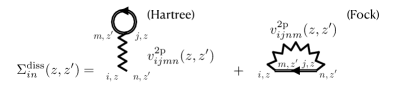
Figure 1: Dissipation-induced self-energy diagrams – oriented double lines represent $G$ and zigzag lines represent $v^{\rm 2p}$. The $(\pm)$ prefactor of the Hartree diagram can be reabsorbed as $\pm v^{\rm 2p}_{ijmn}=v^{\rm 2p}_{ijnm}$, hence $\Sigma^{\rm H}=\Sigma^{\rm F}$. It is readily seen that this is property holds true at any order.

The second term in Eq. (14) is quartic in the field operators and can be treated perturbatively, leading again to a Dyson equation. Unlike physical, e.g., Coulomb, interactions the contour-times $z$ and $z^{\prime}$ are shared by two creation ($\hat{d}^{\dagger}\hat{d}^{\dagger}$) and annihilation ($\hat{d}\hat{d}$) operators rather than by particle-hole-like operators ($\hat{d}^{\dagger}\hat{d}$). This fact gives rise to slightly different self-energy diagrams, with examples provided in Fig. 1. This difference is crucial to show that the number of topological equivalent diagrams of order $k$ is the same as for Coulomb-like interactions, i.e., $2^{k}k!$, despite $v^{\rm 2p}(z,z^{\prime})$ is not symmetric under the exchange $z\leftrightarrow z^{\prime}$. Thus the prefactors of the Feynman diagrams are the same as in ordinary many-body perturbation theory. Taking into account the (anti)symmetry properties of $v^{\rm 2p}$, the Hartree (tadpole) and Fock (oyster) diagrams in Fig. 1 yield the same result, namely $\Sigma^{\rm H}=\Sigma^{\rm F}=\frac{1}{2}\Sigma^{\rm HF}$ with

$$\Sigma^{\rm HF}_{in}(z,z^{\prime}) =\mp 2iv^{\rm 2p}_{ijmn}(z,z^{\prime})G_{mj}(z^{\prime},z)$$

$$=-2i[s(z)\delta(z^{\prime},z)+2\theta_{+}(z)\delta(z^{\prime},\text{\reflectbox{$z$}})]v^{\rm 2p}_{ijmn}(t)\rho^{<}_{mj}(t).$$ (15)

At the Hartree-Fock (HF) mean-field level the r.h.s. of the eom Eq. (8a) is modified by the addition of $\int_{C}d\bar{z}\,\Sigma^{\rm HF}_{in}(z,\bar{z})G_{np}(\bar{z},z^{\prime})=-2v^{\rm 2p}_{ijmn}(t)\rho^{<}_{mj}(t)[is(z)G_{np}(z,z^{\prime})+2i\theta_{-}(\text{\reflectbox{$z$}})G_{np}(\text{\reflectbox{$z$}},z^{\prime})]$. Remarkably, this term renormalizes $\ell^{>}$ in Eqs. (8) according to $\ell^{>}_{in}\to\ell^{>}_{in}+2v^{\rm 2p}_{ijmn}\rho^{<}_{mj}$, while it leaves $\ell^{<}$ unchanged. Such asymmetry is due to the absence of two-body gain. Had we included Lindblad operators of the form $\hat{L}_{\gamma}=b^{\gamma\ast}_{mn}\hat{d}^{\dagger}_{n}\hat{d}^{\dagger}_{m}$ we would have found a similar renormalization for $\ell^{<}$. We infer that the mean-field treatment of two-body loss and gain is equivalent to considering one-body loss and gain.

Particle-hole loss.– The treatment of mixed Lindblad operators, containing both $\hat{d}$ and $\hat{d}^{\dagger}$, deserves a separate discussion, but it does not pose a conceptual problem nor . Let us consider the set $\hat{L}_{\gamma}=a^{\gamma}_{mn}\hat{d}^{\dagger}_{m}\hat{d}_{n}$ (particle-hole loss). As these dissipators are relevant in the context of phonon-induced relaxation of hot electrons in solids Taj et al. (2009); Rosati et al. (2014) we focus on the fermionic case. The normal-ordered form of the operator in Eq. (5) reads

$$\hat{H}(\bar{z},\bar{\text{\reflectbox{$z$}}}) =\hat{H}(\bar{z})-is(z)V^{\rm ph}_{mn}(t)\hat{d}^{\dagger}_{m}(z)\hat{d}_{n}(z)$$

$$+\frac{1}{2}\int_{C}d\bar{z}^{\prime}v^{\rm ph}_{ijmn}(\bar{z},\bar{z}^{\prime})\hat{d}^{\dagger}_{i}(\bar{z}^{\prime+})\hat{d}^{\dagger}_{j}(\bar{z}^{+})\hat{d}_{m}(\bar{z})\hat{d}_{n}(\bar{z}^{\prime}),$$ (16)

where $v^{\rm ph}_{ijmn}(z,z^{\prime})=v^{\rm ph}_{ijmn}(t)[-is(z)\delta(z^{\prime},z)+2i\theta_{-}(z)\delta(z^{\prime},\text{\reflectbox{$z$}})]$, with $v^{\rm ph}_{ijmn}(t)=2a^{\gamma\ast}_{ni}(t)a^{\gamma}_{jm}(t)$, and $V^{\rm ph}_{mn}(t)=\frac{1}{2}v^{\rm ph}_{mjnj}(t)$. The $V^{\rm ph}$-term renormalizes the one-particle Hamiltonian in Eqs. (8) according to $\tilde{h}(z)\to\tilde{h}(z)-is(z)V^{\rm ph}(t)$, but it does not renormalize the function $\ell(z)$. We now show that the mathematical structure of the dissipative KBE is recovered when treating $v^{\rm ph}$ at the HF mean-field level.

For simplicity we take $a^{\gamma\ast}_{mn}=a^{\gamma}_{nm}$. The diagrams with $v^{\rm ph}$ interaction-lines are standard since the contour times $z$ and $z^{\prime}$ are shared by particle-hole-like operators pre . The Hartree (tadpole) diagram is easily shown to vanish whereas the Fock diagram yields

$$\Sigma^{\rm F}_{in}(z,z^{\prime}) =\frac{i}{2}[v^{\rm ph}_{ijnm}(z,z^{\prime})+v^{\rm ph}_{ijnm}(z^{\prime},z)]G_{mj}(z,z^{\prime})$$

$$=s(z)v^{\rm ph}_{ijnm}(t)[\delta(z^{\prime},z)-\delta(z^{\prime},\text{\reflectbox{$z$}})]G_{mj}(z,z^{\prime}).$$ (17)

The r.h.s. of Eq. (9) then reads $[\Sigma^{\rm F}\cdot G]_{ij}^{<}(t,t^{\prime})=2iW^{<}_{in}(t)G^{\rm A}_{nj}(t,t^{\prime})$ where $W^{<}_{in}(t)=\frac{1}{2}v^{\rm ph}_{ipnq}(t)\rho^{<}_{qp}(t)$. This term, together with the $V^{\rm ph}$-renormalization of $\tilde{h}$ leads to a noninteracting dissipative KBE for $G^{<}$ with one-body loss and gain renormalized according to $\ell^{\lessgtr}\to\ell^{\lessgtr}+W^{\lessgtr}$, where $W^{>}=V^{\rm ph}-W^{<}$. Similarly, the r.h.s. of Eq. (10) yields $[G\cdot\Sigma^{\rm F}]^{>}_{ij}(t,t^{\prime})=-2iG^{\rm R}_{in}(t,t^{\prime})W^{>}_{nj}(t^{\prime})+2iG^{>}_{in}(t,t^{\prime})V^{\rm ph}_{nj}(t^{\prime})$. Taking into account the $V^{\rm ph}$-renormalization of $\tilde{h}$ we find a noninteracting dissipative KBE for $G^{>}$ with the same renormalized $\ell^{\lessgtr}$ as for $G^{<}$. Once again, although through a different path, the mean-field treatment reduces the problem to considering one-body loss and gain.

Beyond mean-field.– The self-energy diagrams do, in general, contain both physical and dissipation-induced interaction lines. To derive the KBE we first need to inspect the structure of the total self-energy as a correlator on the Keldysh contour. In Appendix C we show that the total self-energy can be written as $\Sigma=\Sigma^{\rm HF}+\Sigma^{\rm corr}$, where $\Sigma^{\rm HF}$ is the sum of all HF contributions and $\Sigma^{\rm corr}$ satisfies the Keldysh properties. Therefore the Langreth rules remain unchanged and the KBE are still given by Eqs. (9) and (10) with mean-field renormalized $\ell^{\lessgtr}$ and with $\Sigma\to\Sigma^{\rm corr}$.

Conclusions.– The second-quantization approach of NEGF theory has been extended to dissipative Lindbladian dynamics. We have shown how to derive the MSH for the $n$-particle NEGF and established the KBE for $G^{\lessgtr}$. We have generalized the diagrammatic rules for approximate treatments, derived the eom at the mean-field level, and elucidated the structure of the total self-energy as a correlator on the Keldysh contour. We hope that our contribution inspire further developments in the theory of many-body dissipative dynamics and stimulate first-principles studies of driven correlated open systems.

This work has been supported by MIUR PRIN (Grant No. 2022WZ8LME) and INFN through the TIME2QUEST project.

Appendix A Equations of motion

Let $\hat{O}_{i}$ be operators on the Keldysh contour $C$ and consider the contour-ordered string of operators

$$\hat{k}(z_{1},\ldots,z_{n})=\mbox{$\mathcal{T}$}\left\{\hat{O}_{1}(z_{1})\ldots\hat{O}_{n}(z_{n})\right\},$$ (18)

where the contour argument of the operators fixes the position of these operators along the contour, thus rendering unambiguous the action of the contour ordering $\mathcal{T}$. The contour derivative of $\hat{k}$ with respect to the contour-time $z_{k}$ is given by Stefanucci and van Leeuwen (2013)

$$\frac{d}{dz_{k}}\hat{k}(z_{1},\ldots,z_{n}) =\sum_{l\neq k}(-)^{f_{kl}}\delta(z_{k},z_{l})\mbox{$\mathcal{T}$}\left\{\!\hat{O}_{1}\ldots\left[\hat{O}_{k},\hat{O}_{l}\right]_{\mp}\ldots\hat{O}_{n}\!\right\},$$ (19)

where $f_{kl}$ is the number of interchanges of fermionic operators required to bring $\hat{O}_{l}$ to the right of $\hat{O}_{k}$ (if $\hat{O}_{l}$ is a bosonic operator then $f_{kl}=0$ by definition), and the lower sign applies when both $\hat{O}_{k}$ and $\hat{O}_{l}$ are fermionic operators. For a system with general Lindblad operators the NEGF is defined as, see Eq. (6),

$$G_{ij}(z,z^{\prime})=\frac{1}{i}{\rm Tr}\Big{[}\hat{\rho}(0)\mbox{$\mathcal{T}$}\Big{\{}e^{-i\int_{C}d\bar{z}\hat{H}(\bar{z},\bar{\text{\reflectbox{$z$}}})}\hat{d}_{i}(z)\hat{d}^{{\dagger}}_{j}(z^{\prime})\Big{\}}\Big{]}\equiv\frac{1}{i}\left\langle\hat{d}_{i}(z)\hat{d}^{{\dagger}}_{j}(z^{\prime})\right\rangle,$$ (20)

where the operator $\hat{H}(\bar{z},\bar{\text{\reflectbox{$z$}}})$ is given in Eq. (5). Expanding the exponential of Eq. (20) in Taylor series and using Eq. (19) we find

$$i\frac{d}{dz}G_{ij}(z,z^{\prime}) =\delta(z,z^{\prime})+\frac{1}{i}\int_{C}dz_{1}\delta(z,z_{1})\left\langle\left[\hat{d}_{i}(z),\hat{H}(z)-is(z)\hat{L}^{{\dagger}}_{\gamma}(z)\hat{L}_{\gamma}(z)\right]_{-}\hat{d}^{{\dagger}}_{j}(z^{\prime})\right\rangle$$

$$+\frac{1}{i}\int_{C}dz_{1}\delta(z,\text{\reflectbox{$z$}}_{1})2i\theta_{-}(z_{1})\left\langle\left[\hat{d}_{i}(z),\hat{L}^{{\dagger}}_{\gamma}(z)\right]_{\mp}\hat{L}_{\gamma}(z_{1})\hat{d}^{{\dagger}}_{j}(z^{\prime})\right\rangle$$

$$+\frac{1}{i}\int_{C}dz_{1}(\pm)2i\theta_{-}(z_{1})\delta(z,z_{1})\left\langle\hat{L}^{{\dagger}}_{\gamma}(\text{\reflectbox{$z$}}_{1})\left[\hat{d}_{i}(z),\hat{L}_{\gamma}(z)\right]_{\mp}\hat{d}^{{\dagger}}_{j}(z^{\prime})\right\rangle$$

$$=\delta(z,z^{\prime})+\frac{1}{i}\left\langle\left[\hat{d}_{i}(z),\hat{H}(z)-is(z)\hat{L}^{{\dagger}}_{\gamma}(z)\hat{L}_{\gamma}(z)\right]_{-}\hat{d}^{{\dagger}}_{j}(z^{\prime})\right\rangle$$

$$-2\theta_{+}(z)\left\langle\left[\hat{d}_{i}(z),\hat{L}^{{\dagger}}_{\gamma}(z)\right]_{\mp}\hat{L}_{\gamma}(\text{\reflectbox{$z$}})\hat{d}^{{\dagger}}_{j}(z^{\prime})\right\rangle\pm 2\theta_{-}(z)\left\langle\hat{L}^{{\dagger}}_{\gamma}(\text{\reflectbox{$z$}})\left[\hat{d}_{i}(z),\hat{L}_{\gamma}(z)\right]_{\mp}\hat{d}^{{\dagger}}_{j}(z^{\prime})\right\rangle,$$ (21)

where the lower sign applies when both $\hat{d}_{i}$ and $\hat{L}_{\gamma}$ are fermionic operators. In the last identity we use that

$$\int_{\gamma}dzF(z,\text{\reflectbox{$z$}}) =\int_{0}^{\infty}dtF(t_{-},t_{+})+\int_{\infty}^{0}dtF(t_{+},t_{-})=-\int_{0}^{\infty}dtF(t_{+},t_{-})-\int_{\infty}^{0}dtF(t_{-},t_{+})$$

$$=-\int_{\gamma}dzF(\text{\reflectbox{$z$}},z)$$ (22)

for any function $F$. Similarly, we have

$$-i\frac{d}{dz^{\prime}}G_{ij}(z,z^{\prime}) =\delta(z,z^{\prime})-\frac{1}{i}\int_{C}dz_{1}\delta(z^{\prime},z_{1})\left\langle\hat{d}_{i}(z)\left[\hat{d}^{{\dagger}}_{j}(z^{\prime}),\hat{H}(z^{\prime})-is(z^{\prime})\hat{L}^{{\dagger}}_{\gamma}(z^{\prime})\hat{L}_{\gamma}(z^{\prime})\right]_{-}\right\rangle$$

$$-\frac{1}{i}\int_{C}dz_{1}\delta(z^{\prime},\text{\reflectbox{$z$}}_{1})2i\theta_{-}(z_{1})\left\langle\hat{d}_{i}(z)\left[\hat{d}^{{\dagger}}_{j}(z^{\prime}),\hat{L}^{{\dagger}}_{\gamma}(z^{\prime})\right]_{\pm}\hat{L}_{\gamma}(z_{1})\right\rangle$$

$$-\frac{1}{i}\int_{C}dz_{1}\delta(z^{\prime},z_{1})(\pm)2i\theta_{-}(z_{1})\left\langle\hat{d}_{i}(z)\hat{L}^{{\dagger}}_{\gamma}(\text{\reflectbox{$z$}}_{1})\left[\hat{d}^{{\dagger}}_{j}(z^{\prime}),\hat{L}_{\gamma}(z^{\prime})\right]_{\pm}\right\rangle$$

$$=\delta(z,z^{\prime})-\frac{1}{i}\left\langle\hat{d}_{i}(z)\left[\hat{d}^{{\dagger}}_{j}(z^{\prime}),\hat{H}(z^{\prime})-is(z^{\prime})\hat{L}^{{\dagger}}_{\gamma}(z^{\prime})\hat{L}_{\gamma}(z^{\prime})\right]_{-}\right\rangle$$

$$-2\theta_{+}(\text{\reflectbox{$z$}}^{\prime})\left\langle\hat{d}_{i}(z)\left[\hat{d}^{{\dagger}}_{j}(z^{\prime}),\hat{L}^{{\dagger}}_{\gamma}(z^{\prime})\right]_{\pm}\hat{L}_{\gamma}(\text{\reflectbox{$z$}}^{\prime})\right\rangle\mp 2\theta_{-}(z^{\prime})\left\langle\hat{d}_{i}(z)\hat{L}^{{\dagger}}_{\gamma}(\text{\reflectbox{$z$}}^{\prime})\left[\hat{d}^{{\dagger}}_{j}(z^{\prime}),\hat{L}_{\gamma}(z^{\prime})\right]_{\pm}\right\rangle.$$ (23)

For quadratic self-adjoint Hamiltonians $\hat{H}(t)=\hat{H}_{0}(t)=h_{mn}(t)\hat{d}^{{\dagger}}_{m}\hat{d}_{n}$ and linear Lindblad operators $\hat{L}_{1\gamma}(t)=a_{n}^{\gamma}(t)\,\hat{d}_{n}$ (one-body loss) and $\hat{L}_{2\gamma}(t)=b^{\gamma\ast}_{n}(t)\,\hat{d}^{{\dagger}}_{n}$ (one-body gain) the (anti)commutation rules can be used to simplify Eqs. (21) and (23), the final outcome being Eqs. (8). These equations can be written in a more compact form by introducing the two-time matrices

$$\tilde{h}(z_{1},z_{2})=\delta(z_{1},z_{2})\tilde{h}(z_{2})+2i\delta(z_{1},\text{\reflectbox{$z$}}_{2})\ell(z_{2}).$$ (24)

Then

$$i\frac{d}{dz}G(z;z^{\prime})-\int_{C}d\bar{z}\,\tilde{h}(z,\bar{z})G(\bar{z};z^{\prime})=\delta(z,z^{\prime}),$$ (25a)

$$-i\frac{d}{dz^{\prime}}G(z;z^{\prime})-\int_{C}d\bar{z}\,G(z;\bar{z})\tilde{h}(\bar{z},z^{\prime})=\delta(z,z^{\prime}).$$ (25b)

Appendix B Wick’s theorem

Let us define the $n$-particle NEGF according to

$$G_{n}(1,..,n;1^{\prime},..,n^{\prime})=\frac{1}{i}\left\langle\hat{d}(1)..\hat{d}(n)\hat{d}^{{\dagger}}(n^{\prime})..\hat{d}^{{\dagger}}(1^{\prime})\right\rangle,$$ (26)

where $\hat{d}(q)\equiv\hat{d}_{j_{q}}(z_{q})$. This means that $G(1;1^{\prime})=G_{j_{1}j^{\prime}_{1}}(z_{1},z^{\prime}_{1})$. Following the same steps leading to the equations of motion for the one-particle NEGF we find

$$i\frac{d}{dz_{q}}G_{n}(1,..,n;1^{\prime},..,n^{\prime}) -\sum_{k}\int_{C}d\bar{z}\,\tilde{h}_{j_{q}k}(z_{q},\bar{z})G_{n}(1,..,k\bar{z},..,n;1^{\prime},..,n^{\prime})$$

$$=\sum_{l=1}^{n}(\pm)^{l+q}\delta_{j_{q}j^{\prime}_{l}}\delta(z_{q},z^{\prime}_{l})G_{n-1}(1,..,\stackrel{{\scriptstyle\sqcap}}{{q}},..,n;1^{\prime},..,\stackrel{{\scriptstyle\sqcap}}{{l^{\prime}}},..,n^{\prime}),$$ (27)

$$-i\frac{d}{dz^{\prime}_{q}}G_{n}(1,..,n;1^{\prime},..,n^{\prime}) -\sum_{k}\int_{C}d\bar{z}\,G_{n}(1,..,n;1^{\prime},..,k\bar{z},..,n^{\prime})\tilde{h}_{j^{\prime}_{q}k}(\bar{z},z^{\prime}_{q})$$

$$=\sum_{l=1}^{n}(\pm)^{l+q}\delta_{j^{\prime}_{q}j_{l}}\delta(z^{\prime}_{q},z_{l})G_{n-1}(1,..,\stackrel{{\scriptstyle\sqcap}}{{l}},..,n;1^{\prime},..,\stackrel{{\scriptstyle\sqcap}}{{q^{\prime}}},..,n^{\prime}),$$ (28)

where the argument $k\bar{z}$ is placed at position $q$ in Eq. (27) and in position $q^{\prime}$ in Eq. (28). We also introduce the notation according to which the argument underneath the symbol “ $\stackrel{{\scriptstyle\sqcap}}{{}}$ ” is missing. It is easy to verify the validity of Wick’s theorem, i.e.,

$$G_{n}(1,..,n;1^{\prime},..,n^{\prime})=\left|\begin{array}[]{ccc}G(1;1^{\prime})&\ldots&G(1,n^{\prime})\\ \vdots&\vdots&\vdots\\ G(n,1^{\prime})&\ldots&G(n,n^{\prime})\end{array}\right|_{\pm},$$ (32)

where the $\pm$ signifies permanent/determinant. Expanding $G_{n}$ along row $q$:

$$G_{n}(1,..,n;1^{\prime},..,n^{\prime})=\sum_{l=1}^{n}(\pm)^{l+q}G_{j_{q}j^{\prime}_{l}}(z_{q},z^{\prime}_{l})G_{n-1}(1,..,\stackrel{{\scriptstyle\sqcap}}{{q}},..,n;1^{\prime},..,\stackrel{{\scriptstyle\sqcap}}{{l^{\prime}}},..,n^{\prime}).$$ (33)

This expression satisfies Eq. (27) provided that $G_{j_{q}j^{\prime}_{k}}(z_{q},z^{\prime}_{k})$ satisfies Eq. (25a). Similarly, expanding along column $q^{\prime}$

$$G_{n}(1,..,n;1^{\prime},..,n^{\prime})=\sum_{l=1}^{n}(\pm)^{l+q}G_{j_{l}j^{\prime}_{q}}(z_{l};z^{\prime}_{q})G_{n-1}(1,..,\stackrel{{\scriptstyle\sqcap}}{{l}},..,n;1^{\prime},..,\stackrel{{\scriptstyle\sqcap}}{{q^{\prime}}},..,n^{\prime}),$$ (34)

which is easily shown to satisfy Eq. (28) provided that $G_{j_{l}j^{\prime}_{q}}(z_{l},z^{\prime}_{q})$ satisfies Eq. (25b).

Appendix C Self-energy as a correlator on the Keldysh contour

The self-energy diagrams for interacting dissipative systems contain both physical and dissipation-induced interaction lines. For simplicity we here address only two-body loss dissipators; the simultaneous presence of all type of interactions can be worked out along the same line of reasoning.

We consider the set of Lindblad operators (sum of repeated indices is implicit) $\hat{L}_{\gamma}=\sum_{mn}a^{\gamma}_{mn}\hat{d}_{m}\hat{d}_{n}$, with $a^{\gamma}_{mn}=\pm a^{\gamma}_{nm}$ for bosons/fermions. To derive the equations of motionwe need to evaluate the following commutators, see Eqs. (21) and (23),

$$\left[\hat{d}_{i}(z),\hat{H}(z)\right]_{-}=h_{in}(z)\hat{d}_{n}(z),$$ (35)

$$\left[\hat{d}_{i}(z),\hat{L}^{{\dagger}}_{\gamma}(z)\hat{L}_{\gamma}(z)\right]_{-}=v^{\rm 2p}_{iqmn}(t)\hat{d}^{{\dagger}}_{q}(z)\hat{d}_{m}(z)\hat{d}_{n}(z)\equiv\hat{\Theta}_{i}(z),$$ (36)

$$\left[\hat{d}_{i}(z),\hat{L}^{{\dagger}}_{\gamma}(z)\right]_{-}\hat{L}_{\gamma}(\text{\reflectbox{$z$}})=v^{\rm 2p}_{iqmn}(t)\hat{d}^{{\dagger}}_{q}(z)\hat{d}_{m}(\text{\reflectbox{$z$}})\hat{d}_{n}(\text{\reflectbox{$z$}})\equiv\hat{\Delta}_{i}(z).$$ (37)

Taking into account that $\left[\hat{d}_{i}(z),\hat{L}_{\gamma}(z)\right]_{-}=0$ we conclude that (sum over repeated indices is implicit)

$$i\frac{d}{dz}G_{ij}(z,z^{\prime})=\delta(z,z^{\prime})+h_{in}(z)G_{nj}(z,z^{\prime})-s(z)\left\langle\hat{\Theta}_{i}(z)\hat{d}^{{\dagger}}_{j}(z^{\prime})\right\rangle-2\theta_{+}(z)\left\langle\hat{\Delta}_{i}(z)\hat{d}^{{\dagger}}_{j}(z^{\prime})\right\rangle.$$ (38)

Similarly we can extract the adjoint equation of motion. Taking into account that

$$\left[\hat{d}^{{\dagger}}_{j}(z^{\prime}),\hat{H}(z^{\prime})\right]_{-}=-\hat{d}^{{\dagger}}_{m}(z^{\prime})h_{in}(z^{\prime}),$$ (39)

$$\left[\hat{d}^{{\dagger}}_{j}(z^{\prime}),\hat{L}^{{\dagger}}_{\gamma}(z^{\prime})\hat{L}_{\gamma}(z^{\prime})\right]_{-}=\hat{\Theta}^{{\dagger}}_{j}(z^{\prime}),$$ (40)

$$\hat{L}^{{\dagger}}_{\gamma}(\text{\reflectbox{$z$}}^{\prime})\left[\hat{d}^{{\dagger}}_{j}(z^{\prime}),\hat{L}_{\gamma}(z^{\prime})\right]_{-}=\hat{\Delta}^{{\dagger}}_{j}(z^{\prime}),$$ (41)

and that $\left[\hat{d}^{{\dagger}}_{j}(z),\hat{L}^{{\dagger}}_{\gamma}(z)\right]_{-}=0$ we conclude that

$$-i\frac{d}{dz^{\prime}}G_{ij}(z,z^{\prime})=\delta(z,z^{\prime})+G_{im}(z,z^{\prime})h_{mj}(z^{\prime})+s(z^{\prime})\left\langle\hat{d}_{i}(z)\hat{\Theta}^{{\dagger}}_{j}(z^{\prime})\right\rangle-2\theta_{-}(z^{\prime})\left\langle\hat{d}_{i}(z)\hat{\Delta}^{{\dagger}}_{j}(z^{\prime})\right\rangle.$$ (42)

Following the same steps we can calculate the derivative of $\left\langle\hat{\Theta}_{i}(z)\hat{d}^{{\dagger}}_{j}(z^{\prime})\right\rangle$ and $\left\langle\hat{\Delta}_{i}(z)\hat{d}^{{\dagger}}_{j}(z^{\prime})\right\rangle$ with respect to $z^{\prime}$. We see that in Eq. (23) the operator $\hat{d}_{i}(z)$ is a spectator. The result is therefore identical to Eq. (42) with $\hat{d}_{i}(z)\to\hat{\Theta}_{i}(z)$ and $\hat{d}_{i}(z)\to\hat{\Delta}_{i}(z)$, respectively, and the delta function is replaced by $\delta(z,z^{\prime})\left\langle\left[\hat{\Theta}_{i}(z),\hat{d}^{{\dagger}}_{j}(z)\right]_{\mp}\right\rangle$ and $\delta(\text{\reflectbox{$z$}},z^{\prime})\left\langle\left[\hat{\Delta}_{i}(z),\hat{d}^{{\dagger}}_{j}(z)\right]_{\mp}\right\rangle$, respectively. Let us introduce the general correlator on the contour

$$G^{AB}_{ij}(z,z^{\prime}) =\frac{1}{i}\left\langle\hat{A}_{i}(z)\hat{B}^{{\dagger}}_{j}(z^{\prime})\right\rangle.$$ (43)

Then

$$-i\frac{d}{dz^{\prime}}G^{\Theta d}_{ij}(z,z^{\prime})=\delta(z,z^{\prime})\left\langle\left[\hat{\Theta}_{i}(z^{\prime}),\hat{d}^{{\dagger}}_{j}(z^{\prime})\right]_{\mp}\right\rangle+G^{\Theta d}_{ij}(z,z^{\prime})h_{mj}(z^{\prime})+is(z^{\prime})G^{\Theta\Theta}_{ij}(z,z^{\prime})-2i\theta_{-}(z^{\prime})G^{\Theta\Delta}_{ij}(z,z^{\prime}),$$ (44)

$$-i\frac{d}{dz^{\prime}}G^{\Delta d}_{ij}(z,z^{\prime})=\delta(\text{\reflectbox{$z$}},z^{\prime})\left\langle\left[\hat{\Delta}_{i}(\text{\reflectbox{$z$}}^{\prime}),\hat{d}^{{\dagger}}_{j}(z^{\prime})\right]_{\mp}\right\rangle+G^{\Delta d}_{ij}(z,z^{\prime})h_{mj}(z^{\prime})+is(z^{\prime})G^{\Delta\Theta}_{ij}(z,z^{\prime})-2i\theta_{-}(z^{\prime})G^{\Delta\Delta}_{ij}(z,z^{\prime}).$$ (45)

In matrix form Eqs. (38), (42), (44) and (45) read

$$\big{[}i\frac{d}{dz}-h(z)\big{]}G(z,z^{\prime}) =\delta(z,z^{\prime})-is(z)G^{\Theta d}(z,z^{\prime})-2i\theta_{+}(z)G^{\Delta d}(z,z^{\prime}),$$ (46a)

$$G(z,z^{\prime})\big{[}-i\frac{\overleftarrow{d}}{dz^{\prime}}-h(z^{\prime})\big{]} =\delta(z,z^{\prime})+is(z^{\prime})G^{d\Theta}(z,z^{\prime})-2i\theta_{-}(z^{\prime})G^{d\Delta}(z,z^{\prime}),$$ (46b)

$$G^{\Theta d}(z,z^{\prime})\big{[}-i\frac{\overleftarrow{d}}{dz^{\prime}}-h(z^{\prime})\big{]} =\delta(z,z^{\prime})C^{\Theta d}(z^{\prime})+is(z^{\prime})G^{\Theta\Theta}(z,z^{\prime})-2i\theta_{-}(z^{\prime})G^{\Theta\Delta}(z,z^{\prime}),$$ (46c)

$$G^{\Delta d}(z,z^{\prime})\big{[}-i\frac{\overleftarrow{d}}{dz^{\prime}}-h(z^{\prime})\big{]} =\delta(\text{\reflectbox{$z$}},z^{\prime})C^{\Delta d}(z^{\prime})+is(z^{\prime})G^{\Delta\Theta}(z,z^{\prime})-2i\theta_{-}(z^{\prime})G^{\Delta\Delta}(z,z^{\prime}),$$ (46d)

where

$$C^{\Theta d}_{ij}(z) \equiv\left\langle\left[\hat{\Theta}_{i}(z),\hat{d}^{{\dagger}}_{j}(z)\right]_{\mp}\right\rangle=v^{\rm 2p}_{iqmn}(t)\left\langle\left[\hat{d}^{{\dagger}}_{q}(z)\hat{d}_{m}(z)\hat{d}_{n}(z),\hat{d}^{{\dagger}}_{j}(z)\right]_{\mp}\right\rangle=2v^{\rm 2p}_{iqmj}(t)\rho^{<}_{mq}(t),$$

$$C^{\Delta d}_{ij}(z) \equiv\left\langle\left[\hat{\Delta}_{i}(\text{\reflectbox{$z$}}),\hat{d}^{{\dagger}}_{j}(z)\right]_{\mp}\right\rangle=v^{\rm 2p}_{iqmn}(t)\left\langle\left[\hat{d}^{{\dagger}}_{q}(\text{\reflectbox{$z$}})\hat{d}_{m}(z)\hat{d}_{n}(z),\hat{d}^{{\dagger}}_{j}(z)\right]_{\mp}\right\rangle=2v^{\rm 2p}_{iqmj}(t)\left\langle\hat{d}^{{\dagger}}_{q}(\text{\reflectbox{$z$}})\hat{d}_{m}(z)\right\rangle.$$ (47)

From Eq. (46a) we infer that

$$\int d\bar{z}\;\Sigma(z,\bar{z})G(\bar{z},z^{\prime})=-is(z)G^{\Theta d}(z,z^{\prime})-2i\theta_{+}(z)G^{\Delta d}(z,z^{\prime}).$$ (48)

Therefore, acting with $\big{[}-i\frac{\overleftarrow{d}}{dz^{\prime}}-h(z^{\prime})\big{]}$ from the right we get

$$\Sigma(z,z^{\prime})+\int_{C}d\bar{z}d\bar{z}^{\prime}\Sigma(z,\bar{z})G(\bar{z},\bar{z}^{\prime})\Sigma(\bar{z}^{\prime},z^{\prime}) =-is(z)\Big{[}\delta(z,z^{\prime})C^{\Theta d}(z^{\prime})+is(z^{\prime})G^{\Theta\Theta}(z,z^{\prime})-2i\theta_{-}(z^{\prime})G^{\Theta\Delta}(z,z^{\prime})\Big{]}$$

$$-2i\theta_{+}(z)\Big{[}\delta(\text{\reflectbox{$z$}},z^{\prime})C^{\Delta d}(z^{\prime})+is(z^{\prime})G^{\Delta\Theta}(z,z^{\prime})-2i\theta_{-}(z^{\prime})G^{\Delta\Delta}(z,z^{\prime})\Big{]}.$$ (49)

The contribution of the commutators is

$$\Sigma^{\rm HF}_{ij}(z,z^{\prime}) =-is(z)\delta(z,z^{\prime})2v^{\rm 2p}_{iqmj}(t)\rho_{mq}(t)-2i\theta_{+}(z)\delta(\text{\reflectbox{$z$}},z^{\prime})2v^{\rm 2p}_{iqmj}(t)\rho_{mq}(t)$$

$$=-2iv^{\rm 2p}_{iqmj}(t)\rho_{mq}(t)\big{[}s(z)\delta(z,z^{\prime})+2\theta_{+}(z)\delta(\text{\reflectbox{$z$}},z^{\prime})\big{]},$$ (50)

which is exactly the Hartree-Fock contribution arising for the diagrammatic rules, see Eq. (15). Taking into account that $\Sigma G\Sigma$ contributes to the reducible self-energy we conclude that the correlation self-energy is given by

$$\Sigma^{\rm corr}(z,z^{\prime})=\Big{[}s(z)s(z^{\prime})G^{\Theta\Theta}(z,z^{\prime})-2s(z)\theta_{-}(z^{\prime})G^{\Theta\Delta}(z,z^{\prime})+2\theta_{+}(z)s(z^{\prime})G^{\Delta\Theta}(z,z^{\prime})-4\theta_{+}(z)\theta_{-}(z^{\prime})G^{\Delta\Delta}(z,z^{\prime})\Big{]}_{\rm irr}$$ (51)

where the subscript “ irr ” signifies the one-particle irreducible part of the correlators.

Let us prove that this object satisfies the Keldysh properties. We assume $t>t^{\prime}$ and therefore $G^{\Theta\Delta}(z,z^{\prime})=G^{\Delta\Delta}(z,z^{\prime})$ and $G^{\Delta\Theta}(z,z^{\prime})=G^{\Theta\Theta}(z,z^{\prime})$ since $\hat{K}\equiv\mbox{$\mathcal{T}$}\Big{\{}e^{-i\int_{t_{-}}^{t_{+}}d\bar{z}\hat{H}(\bar{z},\bar{\text{\reflectbox{$z$}}})}\Big{\}}=1$. Then setting $z=t_{-}$ and $z^{\prime}=t^{\prime}_{+}$ we get

$$\Sigma^{\rm corr}(t_{-},t^{\prime}_{+})=\Big{[}-G^{\Theta\Theta}(z,z^{\prime})\Big{]}_{\rm irr}.$$ (52)

Let us verify that the result does not change choosing $z=t_{+}$ and $z^{\prime}=t^{\prime}_{+}$ . We get

$$\Sigma^{\rm corr}(t_{+},t^{\prime}_{+})=\Big{[}G^{\Theta\Theta}(z,z^{\prime})-2G^{\Theta\Theta}(z,z^{\prime})\Big{]}_{\rm irr}=\Sigma^{\rm corr}(t_{-},t^{\prime}_{+}).$$ (53)

Next we choose $z=t_{-}$ and $z^{\prime}=t^{\prime}_{-}$. We get

$$\Sigma^{\rm corr}(t_{-},t^{\prime}_{-})=\Big{[}G^{\Theta\Theta}(z,z^{\prime})-2G^{\Delta\Delta}(z,z^{\prime})\Big{]}_{\rm irr}.$$ (54)

On the other hand if we had chosen $z=t_{+}$ and $z^{\prime}=t^{\prime}_{-}$ we would have got

$$\Sigma^{\rm corr}(t_{+},t^{\prime}_{-})=\Big{[}-G^{\Theta\Theta}(z,z^{\prime})+2G^{\Delta\Delta}(z,z^{\prime})+2G^{\Theta\Theta}(z,z^{\prime})-4G^{\Delta\Delta}(z,z^{\prime})\Big{]}_{\rm irr}=\Sigma^{\rm corr}(t_{-},t^{\prime}_{-}).$$ (55)

A similar analysis can be carried out for $t<t^{\prime}$. In this case $G^{\Theta\Delta}(z,z^{\prime})=G^{\Theta\Theta}(z,z^{\prime})$ and $G^{\Delta\Theta}(z,z^{\prime})=G^{\Delta\Delta}(z,z^{\prime})$, and therefore

$$\Sigma^{\rm corr}(t_{-},t^{\prime}_{-})=\Big{[}G^{\Theta\Theta}(z,z^{\prime})-2G^{\Theta\Theta}(z,z^{\prime})\Big{]}_{\rm irr},$$ (56)

$$\Sigma^{\rm corr}(t_{-},t^{\prime}_{+})=\Big{[}-G^{\Theta\Theta}(z,z^{\prime})\Big{]}_{\rm irr}=\Sigma^{\rm corr}(t_{-},t^{\prime}_{-}),$$ (57)

$$\Sigma^{\rm corr}(t_{+},t^{\prime}_{-})=\Big{[}-G^{\Theta\Theta}(z,z^{\prime})+2G^{\Theta\Theta}(z,z^{\prime})+2G^{\Delta\Delta}(z,z^{\prime})-4G^{\Delta\Delta}(z,z^{\prime})\Big{]}_{\rm irr},$$ (58)

$$\Sigma^{\rm corr}(t_{+},t^{\prime}_{+})=\Big{[}G^{\Theta\Theta}(z,z^{\prime})-2G^{\Delta\Delta}(z,z^{\prime})\Big{]}_{\rm irr}=\Sigma^{\rm corr}(t_{+},t^{\prime}_{-}).$$ (59)

In conclusion

$$\Sigma^{\rm corr}(z,z^{\prime})=\theta(z,z^{\prime})\Big{[}G^{\Theta\Theta}(z,z^{\prime})-2G^{\Delta\Delta}(z,z^{\prime})\Big{]}_{\rm irr}-\theta(z^{\prime},z)\Big{[}G^{\Theta\Theta}(z,z^{\prime})\Big{]}_{\rm irr}.$$ (60)