Beamforming Optimization for Active RIS-Aided Multiuser Communications With Hardware Impairments

Abstract

In this paper, we consider an active reconfigurable intelligent surface (RIS) to assist the multiuser downlink transmission in the presence of practical hardware impairments (HWIs), including the HWIs at the transceivers and the phase noise at the active RIS. The active RIS is deployed to amplify the incident signals to alleviate the multiplicative fading effect, which is a limitation in the conventional passive RIS-aided wireless systems. We aim to maximize the sum rate through jointly designing the transmit beamforming at the base station (BS), the amplification factors and the phase shifts at the active RIS. To tackle this challenging optimization problem effectively, we decouple it into two tractable subproblems. Subsequently, each subproblem is transformed into a second order cone programming problem. The block coordinate descent framework is applied to tackle them, where the transmit beamforming and the reflection coefficients are alternately designed. In addition, another efficient algorithm is presented to reduce the computational complexity. Specifically, by exploiting the majorization-minimization approach, each subproblem is reformulated into a tractable surrogate problem, whose closed-form solutions are obtained by Lagrange dual decomposition approach and element-wise alternating sequential optimization method. Simulation results validate the effectiveness of our developed algorithms, and reveal that the HWIs significantly limit the system performance of active RIS-empowered wireless communications. Furthermore, the active RIS noticeably boosts the sum rate under the same total power budget, compared with the passive RIS.

I Introduction

The future sixth generation (6G) of communication systems are anticipated to fulfill the increasing demand for high-quality data transmission and reliable wireless connectivity [1]. Recently, reconfigurable intelligent surface (RIS) has emerged as a prospective technology for 6G networks [2]. The RIS makes the radio propagation environment intelligently reconfigurable, which introduces a notable communication paradigm [3, 4, 5, 2]. In particular, comprising numerous programmable and passive reflecting elements coupled with low power electronics, the RIS can be deployed to establish a virtual line-of-sight link from the source to the destination [2], which is able to improve the coverage and capacity of wireless networks [6, 7, 8]. These appealing characteristics have inspired extensive research works on RIS to improve the performance of traditional communications, including simultaneous wireless information and power transfer (SWIPT) [9], mobile edge computing (MEC) [10], cognitive radio [11], physical layer security [12], visible light communication [13], and unmanned aerial vehicle systems [14] . It has been verified that, with the aid of RISs, the system performance can be improved in terms of various design objectives, e.g., weighted sum rate (WSR) maximization [15], weighted minimum rate maximization [16], energy efficiency maximization in [17], transmit power minimization [18][19], and outage probability minimization [20].

Despite the fact that the aforementioned RIS (i.e., nearly passive RIS) possesses appealing advantages in various aspects, each element reflects the incident signals without performing any signal processing tasks and without signal amplification. The reflected signals, however, suffer from the multiplicative fading effect, resulting in a higher path loss for the reflecting link compared to that of the direct link [21]. Specifically, the signals reflected by a nearly passive RIS are characterized by a cascaded channel, which consists of the source-RIS link and the RIS-destination link [22]. As a consequence, a sufficient number of nearly passive elements is necessary to obtain a high-quality reflected link, which usually results in a large surface size. As a remedy, a novel type of the RIS, named active RIS, has been proposed to mitigate the multiplicative fading effect [23, 24, 25]. Specifically, an active RIS is equipped with active reflection-type amplifiers [23]. Therefore, it has the ability to reflect signals like a nearly passive RIS, and to amplify signals with an additional power supply. The contributions [23, 24, 25, 26, 27, 28] revealed that the performance gain obtained by active RIS outperforms passive RIS under the same total power consumption in most cases. The comparison between active and passive RISs systems in terms of energy efficiency was studied in [29] and [30]. In [31], an active RIS was deployed for improving the secrecy performance by optimizing the transmit beamforming and the reflection coefficients of the active RIS. In [32], the receive beamforming and the reflection coefficients at the active RIS were jointly designed for minimizing the maximum computational latency in the active RIS-empowered MEC systems. An active RIS-aided SWIPT system was explored in [33] to maximize the WSR and weighted sum-power.

It is worth noting that the existing researches about active RIS-aided communications [23, 24, 25, 31, 32, 26, 29, 30, 33, 27, 28] are based on the ideal assumption that both transceivers and active RIS are equipped with perfect hardware. However, in practical communication systems, the hardware impairment (HWI) at the transceivers (T-HWI) is inevitable due to hardware non-linearity and the quantization errors [34]. Unlike the additive noise at the receiver, the T-HWI distorts transmitted and received signals. Although various compensation algorithms were proposed to mitigate the performance degradation caused by HWI [35], it cannot be completely eliminated [34]. Furthermore, owing to the infeasibility of high-precision configuration of RIS phase shifts, the HWI at the RIS (RIS-HWI) is non-negligible, and it is usually modeled as RIS phase noise. Different studies have demonstrated the negative impacts of T-HWI and/or RIS-HWI in passive RIS-assisted communication systems [36, 37, 38, 39, 40, 41]. Specifically, the passive RIS-aided wireless powered Internet of Things network was investigated in [41], revealing that both T-HWI and RIS-HWI resulted in a performance degradation. Accordingly, it is also necessary to take into account both T-HWI and RIS-HWI in active RIS-assisted communication systems. An active RIS-aided device-to-device communication in the presence of RIS-HWI was investigated in [42], the closed-form and asymptotic expressions of the ergodic sum rate were derived. The work in [43] considered an active RIS-assisted single-input-single-output system with RIS-HWI, the effect of which on system performance was analyzed. However, as far as we know, the performance loss caused by both T-HWI and RIS-HWI in active RIS-aided communications remains uninvestigated.

Against this background, we focus on an active RIS-empowered multiuser multiple-input single-output (MISO) communication system in the presence of both T-HWI and RIS-HWI, and we investigate the impact of hardware imperfections on the sum rate performance. The transmit beamforming of the base station (BS) and the reflection coefficients of the active RIS are jointly designed to maximize the sum rate of all users. Different from existing contributions on active RIS-empowered communication networks [23, 24, 25, 31, 32, 26, 29, 30, 33, 27, 28] under the ideal assumption of perfect transceivers hardware and ideal RIS, the non-negligible HWIs at both transceivers and active RIS are taken into account. The problem is challenging to tackle owing to the presence of HWIs and the dynamic noise introduced by active RIS, which cannot be directly addressed with the existing methods. The main contributions of this paper are outlined as below:

• To the best of our knowledge, this is the first attempt to investigate the active RIS-empowered multiuser communications by taking both T-HWI and RIS-HWI into consideration. Specifically, the transmit beamforming and the reflection coefficients are jointly designed for maximizing the sum rate. Nevertheless, the formulated problem is challenging to tackle owing to the non-differentiable nature of the objective function and the strong coupling among the optimization variables.

• To efficiently deal with this sophisticated problem, the original optimization problem is firstly reformulated into an equivalent form through taking advantage of the fractional programming (FP) criterion and quadratic transform. We decouple the original problem into two more tractable subproblems. To be specific, two groups of auxiliary variables are introduced to transform the BS beamforming optimization problem and the active RIS reflection coefficients design problem into second order cone programming (SOCP) problems. Subsequently, the formulated problems are addressed efficiently through invoking the block coordinate descent (BCD) framework, where the optimization variables are alternately updated.

• To further reduce the computational complexity, the minorization-maximization (MM)-based approaches are proposed for deriving a closed-form solution for each subproblem. Based on the classical Lagrangian dual decomposition approach and the MM method, a closed-form solution is derived for the BS beamforming matrix. Then, by exploiting the MM method to simplify the objective function and the constraints, we develop a highly effective element-wise alternating sequential optimization (ASO) approach to achieve a high-quality solution for the reflection coefficients. The designed algorithms can be directly extended to scenarios without taking into account the impact of HWIs, and to the single-user scenarios.

• Extensive simulation results confirm the superiority of active RIS-empowered communications over nearly passive RIS communications in terms of sum rate under the same total power budget. Furthermore, it is indicated that the performance loss caused by HWIs is non-negligible, which unveils the significance of considering both T-HWI and RIS-HWI in active RIS-assisted communications. Finally, the convergence, the effectiveness and the low complexity of the developed approaches are elucidated as well.

The remainder of this paper is organized as follows. We present the system model of an active RIS-empowered multiuser MISO communication system in the presence of HWIs, then the sum rate maximization problem is formulated in Section II, followed by decoupling the original problem into two more tractable subproblems in Section III, then the BCD framework based optimization approach is designed and serves as a benchmark. In Section IV, low-complexity algorithms are developed. Simulation results are shown to confirm the effectiveness of the designed approaches, along with insightful discussions and observations in Section V. Finally, Section VI concludes the paper.

Notations: Constant, vector, matrix are denoted in italic, bold lower case letter, and bold upper case letter, respectively. For a complex value $x$, ${\rm{Re}}\left\{x\right\}$, $\left|x\right|$ and $\angle x$ represent the real part, modulus and angle of $x$, respectively. $(\cdot)^{*}$, $(\cdot)^{T}$, $(\cdot)^{H}$, $(\cdot)^{-1}$ and $(\cdot)^{{\dagger}}$ represent the conjugate, transpose, Hermitian transpose, inverse and pseudo-inverse operations, respectively. ${\rm{Tr}}(\cdot)$, $\left\|\cdot\right\|_{F}$ and ${\rm{vec}}\left(\cdot\right)$ stand for the trace, Frobenius norm and vectorization operator of the input matrix. ${\rm{diag}}(\cdot)$ stands for a diagonal matrix whose diagonal entries are the entries of the input vector. $\widetilde{\rm{diag}}(\cdot)$ represents a diagonal matrix whose diagonal entries are the same as that of the input matrix. For two matrices $\bf{A}$ and $\bf{B}$, ${\bf{A}}\otimes{\bf{B}}$ and ${\bf{A}}\odot{\bf{B}}$ are the Kronecker product and Hadamard product, respectively. ${\nabla}{{f_{\bf{a}}}}({{{{\bf{a}}}}})$ stands for the gradient of the function $f$ w.r.t. $\bf{a}$.

II System Model

II-A System Model

Consider an active RIS-assisted multiuser MISO system, in which an $N$-antenna BS serves $K$ single-antenna users. In this system, an $M$-element active RIS is deployed to enhance the system performance. In particular, to strengthen the reflected signals, each RIS element is integrated with an active reflection-type amplifier supported by the power supply [23]. The phase shift matrix and the amplification matrix of the active RIS are denoted by ${\bf{\Theta}}\buildrel\Delta\over{=}{\rm{diag}}({e^{j{\varphi_{1}}}},\cdots,{e^{j{\varphi_{M}}}})\in{{\mathbb{C}}^{M\times M}}$ and ${\bf{A}}\buildrel\Delta\over{=}{\rm{diag}}\left({{a_{1}},\cdots,{a_{M}}}\right)\in{{\mathbb{R}}_{+}^{M\times M}}$, respectively.

The channel from the BS to the active RIS, the channel for the active RIS to the user $k$, and the direct channel from the BS to the user $k$, are modeled by ${{\bf{G}}}\in{{\mathbb{C}}^{M\times N}}$, ${{\bf{h}}_{k}}\in{{\mathbb{C}}^{M\times 1}}$, ${{\bf{f}}_{k}}\in{{\mathbb{C}}^{N\times 1}}$, respectively, as shown in Fig. 1. Based on the channel estimation techniques in [44, 45, 22, 46], it is assumed that the channel state information (CSI) of all channels is perfectly known at the BS.

II-B HWIs Model

In practice, due to the inherent imperfections of hardware, both the transmitted and the received signals are inevitably subject to the effect of the HWIs, which universally exists in the practical communication systems. In the considered active RIS-aided communication system, the HWIs appear at both transceivers and active RIS. Therefore, there are two different types of HWIs, i.e., T-HWI and RIS-HWI.

For the T-HWI, it is modeled as an independent Gaussian random variable, which causes the mismatch between the received signal and the expected signal, or creates a distortion on the received signal during the reception processing [39]. The power of the distortion noise is proportional to the signal power [34].

For the RIS-HWI, it can be modeled as a random diagonal phase noise matrix, which is denoted as ${\bf{\Phi}}\triangleq{\rm{diag}}\left({\bm{\phi}}\right)$ with ${\bm{\phi}}=\left[{{{\phi_{1}},\ldots,{\phi_{M}}}}\right]^{T}$ and ${\phi_{m}}={e^{j{\vartheta_{m}}}}$. ${\vartheta_{m}}$ is the phase noise at $m$-th element of the active RIS, and it is assumed to be uniformly distributed within $[-\pi/2,\pi/2]$ [39].

II-C Signal Transmission Model

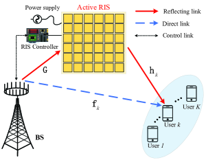
Figure 1: An illustration of an active RIS-assisted multiuser MISO communication system in the presence of transceiver HWIs.

Different from the existing works on active RIS-assisted communications, such as [23, 24, 25, 31, 32, 26, 29, 30, 33, 27, 28], we consider the non-negligible HWIs at both transceivers and active RIS. More specifically, the transmit signal of the BS is

$${{\bf{x}}}={\widehat{\bf{x}}}+{\bm{\eta}_{t}},\ \ \ {\widehat{\bf{x}}}=\sum\limits_{k=1}^{K}{{{\bf{w}}_{k}}{s_{k}}},$$ (1)

where ${\bf{w}}_{k}\in{{\mathbb{C}}^{N\times 1}}$ stands for the beamforming vector adopted by the BS for user $k$, $s_{k}$ denotes the corresponding data symbol with unit power and ${\bm{\eta}_{t}\in{{\mathbb{C}}^{N\times 1}}}$ is the transmit distortion noise, which is independent of $s_{k}$. The variance of each entry in ${\bm{\eta}_{t}}$ is proportional to the transmit power at the corresponding antenna, i.e., $\bm{\eta}_{t}\sim\mathcal{CN}\left({\bm{0},\bm{\Upsilon}_{t}}\right)$, and $\bm{\Upsilon}_{t}$ is expressed as

$$\bm{\Upsilon}_{t}=\kappa_{t}\widetilde{\rm{diag}}\left(\sum\limits_{k=1}^{{K}}{{{{{\bf{w}}_{k}}}{{{\bf{w}}_{k}^{H}}}}}\right),$$ (2)

where $\kappa_{t}\in(0,1)$ is a scale factor which represents the severity of transmitter HWI at the BS.

Then, the signal reflected and amplified by the active RIS is expressed as

$${{\bf{y}}_{\rm RIS}}=\sum\limits_{k=1}^{K}{{\bf{A\Theta\Phi G}}{{\bf{w}}_{k}}{s_{k}}\!+\!{\bf{A\Theta\Phi G}}{{\bm{\eta}}_{t}}\!+\!{\bf{A\Theta\Phi m}}+\bf n},$$ (3)

where the matrix ${\bf{A}}\buildrel\Delta\over{=}{\rm{diag}}\left({{a_{1}},\cdots,{a_{M}}}\right)\in{{\mathbb{R}}_{+}^{M\times M}}$ stands for the amplification matrix, the matrix ${\bf{\Theta}}\buildrel\Delta\over{=}{\rm{diag}}({e^{j{\varphi_{1}}}},\cdots,{e^{j{\varphi_{M}}}})\in{{\mathbb{C}}^{M\times M}}$ represents the phase shift matrix of the active RIS. The vector $\bf{m}$ represents the thermal noise at the active RIS, it cannot be neglected and is modeled as an additive white Gaussian noise (AWGN), whose distribution is ${\bf{m}}\sim{\mathcal{CN}}({\bf{0}}_{M},\sigma_{d}^{2}{{\bf{I}}_{M}})$. The vector $\bf n$ denotes the static noise and it is generally negligible compared to the dynamic noise $\bf A\Theta\Phi m$ [47] . Thus, the signal power at the active RIS can be obtained as

$${P_{{{\bf{y}}_{\rm RIS}}}}= \sum\limits_{k=1}^{K}{{\left\|{{\bf{A\Theta\Phi G}}{{\bf{w}}_{k}}}\right\|}^{2}}+\sigma_{d}^{2}{{\left\|{{\bf{A\Theta\Phi}}}\right\|}^{2}_{F}}$$

$$+{\rm{Tr}}\left({\bf{A\Theta\Phi G}}{\bm{\Upsilon}_{t}}{{\bf{G}}^{H}}{{\bf{\Phi}}^{H}}{{\bf{\Theta}}^{H}}{{\bf{A}}^{H}}\right).$$ (4)

Furthermore, the signal power at the active RIS should not be larger than the amplification power budget $P_{A}$, i.e., ${P_{{{\bf{y}}_{\rm RIS}}}}\leq P_{A}$. Specifically, the amplification power constraint is given by

$${\rm{Tr}}\left({\kappa_{t}}{\bf{A\Theta\Phi G}}\left({{\widetilde{\rm{diag}}}\left({{{{\bf{W}}}{\bf{W}}^{H}}}\right)}\right){{\bf{G}}^{H}}{{\bf{\Phi}}^{H}}{{\bf{\Theta}}^{H}}{{\bf{A}}^{H}}\right)~{}~{}~{}~{}~{}~{}~{}$$

$$~{}~{}~{}~{}~{}~{}~{}~{}~{}~{}~{}~{}~{}~{}~{}~{}~{}+{{\left\|{{\bf{A\Theta\Phi G}}{{\bf{W}}}}\right\|}^{2}_{F}}+\sigma_{d}^{2}{{\left\|{{\bf{A\Theta\Phi}}}\right\|}^{2}_{F}}\leq{P_{A}}.$$ (5)

Furthermore, the received signal at user $k$ is

$${y_{k}}= \underbrace{{\bf{g}}_{k}^{H}{{\bf{w}}_{k}}{s_{k}}}_{{\text{Desired~{} signal}}}+\underbrace{{\bf{g}}_{k}^{H}{{\bm{\eta}}_{t}}}_{{\text{Transmitter~{}HWI}}}+\underbrace{{\bf{g}}_{k}^{H}\sum\limits_{i=1,i\neq k\hfill}^{K}{{{\bf{w}}_{i}}{s_{i}}}}_{{\text{Multiuser~{} interference}}}$$

$$+\underbrace{{\bf{h}}_{k}^{H}{\bf{A\Theta\Phi m}}}_{{\text{Dynamic~{}noise}}}+\underbrace{{n_{k}}}_{{\text{Noise ~{}at~{}user}}~{}k}+\underbrace{{\eta_{r,k}}}_{{\text{Receiver~{}HWI}}},$$ (6)

where ${\bf{g}}_{k}^{H}\triangleq\left({{\bf{h}}_{k}^{H}{\bf{A\Theta\Phi G}}+{\bf{f}}_{k}^{H}}\right)\in{{\mathbb{C}}^{1\times N}}$, ${n_{k}}$ stands for the AWGN at user $k$ with distribution of $\mathcal{CN}(0,\sigma_{k}^{2})$. We denote ${y_{k}}\triangleq\widetilde{{y}}_{k}+{\eta_{r,k}}$, where ${\eta_{r,k}}$ denotes the receive distortion noise at user $k$, which is independent of ${\widetilde{{y}}}_{k}$. Note that the variance of ${\eta_{r,k}}$ is proportional to the power of received signal. Hence, we have ${\eta_{r,k}}\sim\mathcal{CN}(0,{\gamma_{r,k}})$. Here, ${\gamma_{r,k}}$ is given by ${\gamma_{r,k}}=\kappa_{r,k}\mathbb{E}\left\{{{\left|\widetilde{y}_{k}\right|}^{2}}\right\}$, where $\kappa_{r,k}\in(0,1)$ is a scale factor which accounts for the severity of the receiver HWI at the user $k$.

Correspondingly, according to (II-C), the SINR at user $k$ can be obtained as Equation (7) at the top of this page.

$$\!\!\!{\gamma_{k}}\!=\!\frac{{{{\left|{{\bf{g}}_{k}^{H}{{\bf{w}}_{k}}}\right|}^{2}}}}{{{\bf{g}}_{k}^{H}\!\left({{\kappa_{r,k}}{{\bf{w}}_{k}}{\bf{w}}_{k}^{H}\!+\!\left({1\!+\!{\kappa_{r,k}}}\right){\kappa_{t}}\widetilde{\rm{diag}}\left({\sum\limits_{k=1}^{K}{{{\bf{w}}_{k}}{\bf{w}}_{k}^{H}}}\right)}\right){{\bf{g}}_{k}}\!+\!\left({1\!+\!{\kappa_{r,k}}}\right)\!\!\left(\!\sum\limits_{\scriptstyle i=1\hfill\atop\scriptstyle i\neq k\hfill}^{K}\!\!\!{{{\left|{{\bf{g}}_{k}^{H}{{\bf{w}}_{i}}}\right|}^{2}}}\!+\!\sigma_{d}^{2}{{\left\|{{\bf{h}}_{k}^{H}{\bf{A\Theta\Phi}}}\right\|}^{2}}\!+\!\sigma_{k}^{2}\right)}}$$ (7)

Therefore, the data rate (bps/Hz) of user $k$ is expressed as

$${R_{k}}={\log}_{2}\left({1+{\gamma_{k}}}\right).$$ (8)

II-D Total Power Consumption Model

The total power budget for the considered active RIS-empowered system is composed of the transmit power of the BS, the amplification power of the active RIS, the hardware static power of the BS and of the active RIS [17, 30]. To sum up, the total power budget of the active RIS-empowered communication system is given by

$${P_{tot}}={\xi_{T}}{P_{T}}+{\xi_{A}}{P_{A}}+{P_{{\rm{BS}}}}+{P_{{\rm{RIS}}}},$$ (9)

where ${\xi_{T}}\triangleq\nu_{T}^{-1}$ and ${\xi_{A}}\triangleq\nu_{\rm{A}}^{-1}$ with $\nu_{\rm{T}}\in(0,1]$ and $\nu_{\rm{A}}\in(0,1]$ being the efficiency of the transmit power amplifiers and the efficiency of the active RIS amplifiers, respectively. $P_{T}$ represents the transmit power at the BS in the active RIS system. ${P_{{\rm{BS}}}}$ and ${P_{{\rm{RIS}}}}$ represent the hardware static power of the BS and of the active RIS, respectively. In particular, the static power of active RIS depends on the number of elements. Therefore, the static power dissipated at an active RIS with $M$ elements can be expressed as ${P_{{\rm{RIS}}}}=M\left({{P_{{\rm{SW}}}}+{P_{{\rm{DC}}}}}\right)$, where ${P_{{\rm{SW}}}}$ and ${P_{{\rm{DC}}}}$ represent the control circuit power and the direct current (DC) biasing power consumed by each active RIS element, respectively [25].

II-E Phase Noise Processing

Due to the randomness of the phase noise matrix, it is difficult to obtain the exact expression for the date rate. Inspired by [48, 39, 49], we exploit the expectation to take over the randomness of $\bf\Phi$. Then, the average phase distortion level [50] at the active RIS can be calculated to obtain the approximate average rate.

By adopting [48, Lemma 1], we have

$${R_{k}}\approx{\widetilde{R}_{k}}={\log_{2}}\left({1+\widetilde{{\gamma}}}_{k}\right),$$ (10)

where ${\widetilde{R}}_{k}$ denotes the approximate average rate [39], and

$$\widetilde{{\gamma}}_{k}= \frac{{{\varpi_{1}}}}{{{\varpi_{2}}+{\varpi_{3}}-{\varpi_{1}}}},$$ (11)

$${\varpi_{1}}\triangleq {\mathbf{w}}_{k}^{H}{\mathbb{E}_{\mathbf{\Phi}}}\left\{{{{\mathbf{g}}_{k}}{\mathbf{g}}_{k}^{H}}\right\}{{\mathbf{w}}_{k}},$$ (12)

$${\varpi_{2}}\triangleq \left({1+{\kappa_{r,k}}}\right){\text{Tr}}\left(\left({\sum\limits_{k=1}^{K}{{{\mathbf{w}}_{k}}{\mathbf{w}}_{k}^{H}}+{\kappa_{t}}\widetilde{{\text{diag}}}\left({\sum\limits_{k=1}^{K}{{{\mathbf{w}}_{k}}{\mathbf{w}}_{k}^{H}}}\right)}\right)\right.$$

$$\times{\mathbb{E}_{\mathbf{\Phi}}}\left\{{{{\mathbf{g}}_{k}}{\mathbf{g}}_{k}^{H}}\right\}\Big{)},$$ (13)

$${\varpi_{3}}\triangleq {\mathbb{E}_{\mathbf{\Phi}}}\left\{{\left({1+{\kappa_{r,k}}}\right)\left({\sigma_{d}^{2}{{\left\|{{\mathbf{h}}_{k}^{H}{\mathbf{A\Theta\Phi}}}\right\|}^{2}}+\sigma_{k}^{2}}\right)}\right\}.$$ (14)

Furthermore, ${\mathbb{E}_{\bf{\Phi}}\left\{{{{\bf{g}}_{k}}{\bf{g}}_{k}^{H}}\right\}}$ can be calculated as follows.

$$\!\!\!{\mathbb{E}_{\bf{\Phi}}\left\{{{{\bf{g}}_{k}}{\bf{g}}_{k}^{H}}\right\}}$$

$$={{\bf{G}}^{H}}{{{\bf{\Theta}}^{H}}{{\bf{A}}^{H}}}{\rm{diag}}\left({{{\bf{h}}_{k}}}\right){{\mathbb{E}}_{\bm{\phi}}}\left\{{{\bm{\phi}}{{\bm{\phi}}^{H}}}\right\}{\rm{diag}}\left({{\bf{h}}_{k}^{H}}\right){\bf{A\Theta G}}$$

$$+2{\mathop{\rm Re}\nolimits}\left\{{{{\bf{G}}^{H}}{{{\bf{\Theta}}^{H}}{{\bf{A}}^{H}}}{\rm{diag}}\left({{{\bf{h}}_{k}}}\right){{\mathbb{E}}_{\bm{\phi}}}\left\{{{{\bm{\phi}}^{*}}}\right\}{\bf{f}}_{k}^{H}}\right\}+{{\bf{f}}_{k}}{\bf{f}}_{k}^{H}.$$ (15)

To further calculate ${\mathbb{E}_{\bf{\Phi}}\left\{{{{\bf{g}}_{k}}{\bf{g}}_{k}^{H}}\right\}}$, we first need to obtain ${{\mathbb{E}}_{\bm{\phi}}}\left\{{{{\bm{\phi}}{\bm{\phi}}^{H}}}\right\}$ and ${{\mathbb{E}}_{\bm{\phi}}}\left\{{{{\bm{\phi}}^{*}}}\right\}$. Denote $\delta_{\vartheta}=\vartheta_{i}-\vartheta_{j},\forall i,j=1,2,\cdots,M$. Note that $\vartheta_{i}$ and $\vartheta_{j}$ are uniformly distributed within $[-\pi/2,\pi/2]$, their probability density function can be expressed as $f\left(\vartheta_{i}\right)=\frac{1}{\pi}$. Thus, $\delta_{\vartheta}$ obeys triangular distribution on $[-\pi,\pi]$, and its probability density function can be expressed as [39]

$$f\left(\delta_{\vartheta}\right)=\begin{cases}\frac{1}{\pi^{2}}\delta_{\vartheta}+\frac{1}{\pi},&\delta_{\vartheta}\in\left[-\pi,0\right],\\ -\frac{1}{\pi^{2}}\delta_{\vartheta}+\frac{1}{\pi},&\delta_{\vartheta}\in\left[0,\pi\right].\\ \end{cases}$$ (16)

Therefore, we have $\mathbb{E}_{\delta_{\vartheta}}\left\{e^{j\vartheta_{i}-j\vartheta_{j}}\right\}=\mathbb{E}_{\delta_{\vartheta}}\left\{e^{j\delta_{\vartheta}}\right\}=\int_{-\pi}^{\pi}{f\left(\delta_{\vartheta}\right)}e^{j\delta_{\vartheta}}d\delta_{\vartheta}=\frac{4}{\pi^{2}}$, and $\mathbb{E}_{\bm{\phi}}\left\{\bm{\phi}\bm{\phi}^{H}\right\}$ can be given by

$$\mathbb{E}_{\bm{\phi}}\left\{\bm{\phi}\bm{\phi}^{H}\right\} =\left(\begin{matrix}1&\cdots&\mathbb{E}_{\delta_{\vartheta}}\left\{e^{j\vartheta_{M}-j\vartheta_{1}}\right\}\\ \mathbb{E}_{\delta_{\vartheta}}\left\{e^{j\vartheta_{1}-j\vartheta_{2}}\right\}&\cdots&\mathbb{E}_{\delta_{\vartheta}}\left\{e^{j\vartheta_{M}-j\vartheta_{2}}\right\}\\ \vdots&\ddots&\vdots\\ \mathbb{E}_{\delta_{\vartheta}}\left\{e^{j\vartheta_{1}-j\vartheta_{M}}\right\}&\cdots&1\\ \end{matrix}\right)$$

$$=\mathbf{I}_{M}+\mathbf{J},$$ (17)

where

$${\left[{\bf{J}}\right]_{(i,j)}}=\left\{{\begin{array}[]{*{20}{c}}{0,~{}~{}~{}~{}i=j,}\\ {\frac{4}{{{\pi^{2}}}},~{}~{}i\neq j.}\end{array}}\right.$$ (20)

Furthermore, to calculate ${{\mathbb{E}}_{\bm{\phi}}}\left\{{{{\bm{\phi}}^{*}}}\right\}$, we can obtain $\mathbb{E}_{\vartheta_{i}}\left\{e^{-j\vartheta_{i}}\right\}=\int_{-\frac{\pi}{2}}^{\frac{\pi}{2}}{f\left(\vartheta_{i}\right)}\left(\cos\vartheta_{i}-j\sin\vartheta_{i}\right)d\vartheta_{i}=\frac{2}{\pi}$. Then, we have

$$\mathbb{E}_{\bm{\phi}}\left\{\bm{\phi}^{*}\right\}=\frac{2}{\pi}{\mathbf{1}}_{M},$$ (21)

where ${\mathbf{1}}_{M}$ stands for the unit column vector with all elements being one.

By substituting (17) and (21) into (15), we have

$$\mathbb{E}_{\bf{\Phi}} \left\{{{{\bf{g}}_{k}}{\bf{g}}_{k}^{H}}\right\}$$

$$= {{\bf{G}}^{H}}{{{\bf{\Theta}}^{H}}{{\bf{A}}^{H}}}{\rm{diag}}\left({{{\bf{h}}_{k}}}\right)\left({{{\bf{I}}_{M}}+{\bf{J}}}\right){\rm{diag}}\left({{\bf{h}}_{k}^{H}}\right){\bf{A\Theta G}}$$

$$+2{\mathop{\rm Re}\nolimits}\left\{{{{\bf{G}}^{H}}{{{\bf{\Theta}}^{H}}{{\bf{A}}^{H}}}{\rm{diag}}\left({{{\bf{h}}_{k}}}\right)\frac{2}{\pi}{{\bf{1}}_{M}}{\bf{f}}_{k}^{H}}\right\}+{{\bf{f}}_{k}}{\bf{f}}_{k}^{H}$$

$$= {{\bf{G}}^{H}}{{{\bf{\Theta}}^{H}}{{\bf{A}}^{H}}}{\rm{diag}}\left({{{\bf{h}}_{k}}}\right){\bf{D}}{{\bf{D}}^{T}}{\rm{diag}}\left({{\bf{h}}_{k}^{H}}\right){\bf{A\Theta G}}$$

$$+\left({\frac{2}{\pi}{{\bf{G}}^{H}}{{{\bf{\Theta}}^{H}}{{\bf{A}}^{H}}}{{\bf{h}}_{k}}+{{\bf{f}}_{k}}}\right)\left({\frac{2}{\pi}{\bf{h}}_{k}^{H}{\bf{A\Theta G}}+{\bf{f}}_{k}^{H}}\right)$$

$$= {\widehat{\bf{f}}_{k}}\widehat{\bf{f}}_{k}^{H}+{\widehat{\bf{G}}_{k}}\widehat{\bf{G}}_{k}^{H}={\overline{\bf{G}}_{k}}\overline{\bf{G}}_{k}^{H},$$ (22)

where ${\overline{\bf{G}}_{k}}\triangleq\left[{{{\widehat{\bf{f}}}_{k}},{{\widehat{\bf{G}}}_{k}}}\right]\in\mathbb{C}^{N\times(1+M)}$, $\widehat{\bf{f}}_{k}^{H}\triangleq\frac{2}{\pi}{\bf{h}}_{k}^{H}{\bf{A\Theta G}}+{\bf{f}}_{k}^{H}$, $\widehat{\bf{G}}_{k}^{H}\triangleq{{\bf{D}}^{T}}{\rm{diag}}\left({{\bf{h}}_{k}^{H}}\right){\bf{A\Theta G}}$ and ${\bf{D}}{{\bf{D}}^{T}}\triangleq{\rm{diag}}\left({\left({1-\frac{4}{{{\pi^{2}}}}}\right){{\bf{I}}_{M}}}\right)$. Therefore, the approximate average rate can be written as ${\widetilde{R}_{k}}={\log_{2}}\left({1+\widetilde{{\gamma}}}_{k}\right)$, where

$$\widetilde{{\gamma}}_{k}= \frac{\widetilde{{\varpi_{1}}}}{{\widetilde{{\varpi_{2}}}+\widetilde{{\varpi_{3}}}-\widetilde{{\varpi_{1}}}}},$$ (23)

$$\widetilde{{\varpi_{1}}}\triangleq {{\bf{w}}_{k}^{H}{{\overline{\bf{G}}}_{k}}\overline{\bf{G}}_{k}^{H}{{\bf{w}}_{k}}},$$ (24)

$$\widetilde{{\varpi_{2}}}\triangleq \left({1\!+\!{\kappa_{r,k}}}\right){\rm{Tr}}\left({\left({{\bf{W}}{{\bf{W}}^{\rm{H}}}\!+\!{\kappa_{\rm{t}}}\widetilde{{\rm{diag}}}\left({{\bf{W}}{{\bf{W}}^{\rm{H}}}}\right)}\right){{\overline{\bf{G}}}_{k}}\overline{\bf{G}}_{k}^{H}}\right),$$ (25)

$$\widetilde{{\varpi_{3}}}\triangleq \left({1+{\kappa_{r,k}}}\right)\times$$

$$\big{(}{\sigma_{d}^{2}{\rm{Tr}}\left({{{{\bf{\Theta}}^{H}}{{\bf{A}}^{H}}}{\rm{diag}}\left({{{\bf{h}}_{k}}}\right)\left({{{\bf{I}}_{M}}+{\bf{J}}}\right){\rm{diag}}\left({{\bf{h}}_{k}^{H}}\right){\bf{A\Theta}}}\right)+\sigma_{k}^{2}}\big{)}.$$ (26)

II-F Problem Formulation

In this work, we aim for jointly designing the beamforming matrix at the BS, the amplification matrix and the phase shift matrix at the active RIS, i.e., $\{{\bf{W}},{\bf{A}},{\bf{\Theta}}\}$, to maximize the sum rate. Different from the nearly passive RIS design in prior works, the amplifiers at the active RIS introduce amplification power constraints rather than the unit modulus constraints. Therefore, the optimization problem can be formulated as

$$\!\!\!\!\!\!\mathop{{\rm{max}}}\limits_{{{\bf{W}}},{\bf{A}},{\bf{\Theta}}}~{}~{}~{} {\sum\limits_{k=1}^{K}{{\widetilde{R}_{k}}}}$$ (27a)

$${\rm{s.}}{\rm{t.}}~{}~{}~{}~{}~{} {\rm{Tr}}\left({{\bf{W}}{{\bf{W}}^{H}}}\right)\leq{P_{T}},$$ (27b)

$${P_{{{\bf{y}}_{\rm RIS}}}}\leq{P_{A}},$$ (27c)

where ${\bf{W}}\buildrel\Delta\over{=}[{\bf{w}}_{1},\dots,{\bf{w}}_{K}]\in{{\mathbb{C}}^{N\times K}}$. Obviously, Problem (27) is non-convex thanks to the coupled optimization variables. Furthermore, compared with nearly passive RIS, active RIS also introduces additional dynamic noise term, which makes the objective function more difficult. Compared to the corresponding scenario without HWI, the objective function and the constraints of Problem (27) become more sophisticated. Consequently, Problem (27) cannot be readily addressed through the existing approaches. In what follows, we propose efficient algorithms to solve it.

III BCD-SOCP Algorithm

In this section, to decouple the BS beamforming variables and the RIS reflection coefficient variables, Problem (27) is firstly reformulated into a more tractable equivalent form with the aid of the FP method. Then, two subproblems are alternately solved by exploiting the BCD framework.

III-A Problem Reformulation

To solve the non-convex problem effectively, the original Problem (27) is reformulated by means of the FP approach [51], where the optimization variables are decoupled. Notice that the amplification matrix ${\bf{A}}$ and the phase shift matrix ${\bf{\Theta}}$ always present in a product form, it can be expressed as ${\bf{\Psi}}={\bf{A\Theta}}={\rm{diag}}\left({{a_{1}}{e^{j{\varphi_{1}}}},\cdots,{a_{M}}{e^{j{\varphi_{M}}}}}\right)\in{{\mathbb{C}}^{M\times M}}$. Then, we introduce a lemma as below.

Lemma 1

Upon introducing two groups of auxiliary variables ${\mathcal{U}}=\left\{{{{\bf u}_{k}}\in{\mathcal{U}},\forall k\in{\mathcal{K}}}\right\}$ and ${\mathcal{V}}=\left\{{{v_{k}}\in{\mathcal{V}},\forall k\in{\mathcal{K}}}\right\}$, and adopting the quadratic transform [51], Problem (27) is equivalently reformulated as

$$\mathop{{\rm{max}}}\limits_{{{\bf{W}},{\bf{\Psi}},{\mathcal{U}},\mathcal{V}}}~{}~{}~{} {\sum\limits_{k=1}^{K}{r_{k}}\left({{\bf{W}},{\bf{\Psi}},{\mathcal{U}},\mathcal{V}}\right)}$$ (28a)

$${\rm{s.}}{\rm{t.}}~{}~{}~{}~{}~{} {\rm{Tr}}\left({{\bf{W}}{{\bf{W}}^{H}}}\right)\leq{P_{T}},$$ (28b)

$${P_{{{\bf{y}}_{\rm RIS}}}}\leq{P_{A}},$$ (28c)

where $\mathop{\max}\limits_{{\cal U},{\cal V}}\left\{{{r_{k}}\left({{\bf{W}},{\bf{\Psi}},{\cal U},{\cal V}}\right)}\right\}=\frac{1}{{{{\log}_{2}}e}}\widetilde{{R}}_{k}$ holds, and

$$\!\!\!\!{r_{k}}\left({{\bf{W}},{\bf{\Psi}},{\mathcal{U}},\mathcal{V}}\right)= \log\left({1+{v_{k}}}\right)\!-\!{v_{k}}$$

$$+2\sqrt{\left({1+{v_{k}}}\right)}{\mathop{\rm Re}\nolimits}\left\{{{\bf{u}}_{k}^{H}\overline{\bf{G}}_{k}^{H}{{\bf{w}}_{k}}}\right\}\!-\!{\bf{u}}_{k}^{H}{{\bf{u}}_{k}}{\widetilde{{\varpi_{2}}}}-{\bf{u}}_{k}^{H}{{\bf{u}}_{k}}{\widetilde{{\varpi_{3}}}},$$ (29)

$${\bf u}_{k}^{\star}= ~{}\frac{{\sqrt{\left({1+{v_{k}}}\right)}~{}\overline{\bf{G}}_{k}^{H}{{\bf{w}}_{k}}}}{{\widetilde{{\varpi_{2}}}+\widetilde{{\varpi_{3}}}}}\in{\mathbb{C}}^{\left({M+1}\right)\times 1},$$ (30)

$$v_{k}^{\star}= ~{}\frac{\widetilde{{\varpi_{1}}}}{{\widetilde{{\varpi_{2}}}+\widetilde{{\varpi_{3}}}-\widetilde{{\varpi_{1}}}}}.$$ (31)

Compared with the original objective function of Problem (27), the objective function of Problem (28) is more tractable, although more optimization variables are introduced. To deal with Problem (28), we develop the BCD method to maximize the objective function in Problem (27) by alternately designing each group of variables, while the other groups of variables keep fixed. Since the optimal ${{\bf u}_{k}}$ and optimal ${v_{k}}$ in each iteration can be obtained in (30) and (31), respectively, the remaining task is to design the BS beamforming matrix $\bf{W}$ as well as the RIS reflection coefficient matrix ${\bf{\Psi}}$. Let us focus on optimizing ${\bf{W}}$ and ${\bf{\Psi}}$ in the following.

III-B Optimize the BS Beamforming Matrix $\bf{W}$

In this subsection, the BS beamforming matrix $\bf{W}$ is optimized while keeping ${\bf{\Psi}},~{}{\mathcal{U}}$ and $\mathcal{V}$ fixed. Denote ${\bf{w}}\buildrel\Delta\over{=}{{\rm{vec}}{(\bf W)}}$ and introduce a selection vector $t_{k}\in{\mathbb{R}}^{K\times 1}$, where all elements are zero except for the $k$-th element, which is one. Then, Lemma 2 is introduced.

Lemma 2

For a fixed RIS reflection coefficient matrix ${\bf{\Psi}}$ and auxiliary variables ${\mathcal{U}}$ and ${\mathcal{V}}$, the subproblem for the optimization of the BS beamforming vector $\bf{w}$ is transformed into an equivalent problem as follows:

$$\mathop{{\rm{min}}}\limits_{{{\bf{w}}}}~{}~{}~{} {{{\bf{w}}^{H}}{\bf{\tilde{\Xi}w}}-2{\rm{Re}}\left\{{{{\bm{\omega}}^{H}}{\bf{w}}}\right\}-c}$$ (32a)

$${\rm{s.}}{\rm{t.}}~{}~{}~{} {{\bf{w}}^{H}{{\bf{w}}}}\leq{P_{T}},$$ (32b)

$${{{\bf{w}}^{H}}{\bf{\Gamma w}}}\leq{P_{m}},$$ (32c)

where

$${\bm{\omega}}\triangleq \sum\limits_{k=1}^{K}{{\text{vec}}\left({{\mathbf{\Omega}}_{k}^{H}}\right)}\in{\mathbb{C}^{NK\times 1}},$$ (33)

$$\widetilde{\mathbf{\Xi}}\triangleq \sum\limits_{k=1}^{K}{\left({{{\mathbf{I}}_{K}}\otimes{{\mathbf{\Xi}}_{k}}}\right)}\in{{\mathbb{C}}^{NK\times NK}},$$ (34)

$${{\mathbf{\Omega}}_{k}}\triangleq \sqrt{\left({1+{v_{k}}}\right)}{{\mathbf{t}}_{k}}{\mathbf{u}}_{k}^{H}\overline{\mathbf{G}}_{k}^{H},$$ (35)

$${{\mathbf{\Xi}}_{k}}\triangleq \left({1+{\kappa_{{\text{r,}}k}}}\right){\mathbf{u}}_{k}^{H}{{\mathbf{u}}_{k}}\left({{{\overline{\mathbf{G}}}_{k}}\overline{\mathbf{G}}_{k}^{H}+{\kappa_{\text{t}}}\widetilde{{\rm{diag}}}\left({{{\overline{\mathbf{G}}}_{k}}\overline{\mathbf{G}}_{k}^{H}}\right)}\right),$$ (36)

$${c_{k}}\triangleq \sum\limits_{k=1}^{K}\big{(}{\log\left({1+{v_{k}}}\right)-{v_{k}}-\left({1+{\kappa_{r,k}}}\right){\mathbf{u}}_{k}^{H}{{\mathbf{u}}_{k}}\times}$$

$${\left({\sigma_{d}^{2}{\text{Tr}}\left({{{\bf{\Psi}}^{H}}{\rm{diag}}\left({{{\bf{h}}_{k}}}\right)\!\left({{{\mathbf{I}}_{M}}+{\mathbf{J}}}\right){\rm{diag}}\left({{\mathbf{h}}_{k}^{H}}\right){\mathbf{\Psi}}}\right)\!+\!\sigma_{k}^{2}}\right)}\big{)},$$ (37)

$${\bf{\Gamma}}\triangleq {{\bf{I}}_{K}}\otimes\left({{\bf{G}}^{H}}{{\bf{\Psi}}^{H}}{\bf{\Psi G}}+{\kappa_{t}}{\widetilde{\rm{diag}}}\left({{{\bf{G}}^{H}}{{\bf{\Psi}}^{H}}{\bf{\Psi G}}}\right)\right),$$ (38)

$${P_{m}}\triangleq {P_{A}}-\sigma_{d}^{2}{\left\|{\bf{\Psi}}\right\|^{2}_{F}}.$$ (39)

The reformulation in (32) is an SOCP problem, which can be tackled through exploiting the standard optimization packages, such as CVX [52].

III-C Optimize the RIS Reflection Coefficient Matrix ${\bf{\Psi}}$

In this subsection, the RIS reflection coefficient matrix $\bf{\Psi}$ is optimized while ${\bf{W}},~{}{\mathcal{U}}$ and $\mathcal{V}$ are kept fixed. Define ${\bm{\psi}}=\left[{{a_{1}}{e^{j{\varphi_{1}}}},\cdots,{a_{M}}{e^{j{\varphi_{M}}}}}\right]^{T}\in{\mathbb{C}}^{M\times 1}$ as the diagonal entries of ${\bf{\Psi}}$, i.e., ${\bf{\Psi}}={\rm{diag}}({\bm{\psi}})$. Then, we introduce a lemma as below.

Lemma 3

For a fixed BS beamforming matrix ${\bf{W}}$ and auxiliary variables ${\mathcal{U}}$ and ${\mathcal{V}}$, the subproblem for the optimization of active RIS reflection coefficient vector ${\bm{\psi}}$ is equivalently transformed into the following form:

$$\mathop{{\rm{min}}}\limits_{{{\bm{\psi}}}}~{}~{}~{} {{\bm{\psi}}^{H}}{\bf{\Delta}}{\bm{\psi}}-2{\mathop{\rm Re}\nolimits}\left\{{{\bm{\psi}}^{H}{{\bm{\alpha}}}}\right\}-d$$ (40a)

$${\rm{s.}}{\rm{t.}}~{}~{}~{} {{\bm{\psi}}^{H}}{\bf{\Lambda}}{\bm{\psi}}\leq{P_{A}},$$ (40b)

where

$${\mathbf{\Delta}}\triangleq \sum\limits_{k=1}^{K}{\left({{{\mathbf{\Delta}}_{1,k}}+{{\mathbf{\Delta}}_{2,k}}}\right)},$$ (41)

$${{\bm{\alpha}}^{H}}\triangleq \sum\limits_{k=1}^{K}{\left({\sqrt{\left({1+{v_{k}}}\right)}{\bm{\alpha}}_{1,{\bm{\psi}},k}^{H}-{\bm{\alpha}}_{2,{\bm{\psi}},k}^{H}}\right)}$$ (42)

$${{\mathbf{Q}}_{k}}\triangleq {\mathbf{u}}_{k}^{H}{{\mathbf{u}}_{k}}\left({1+{\kappa_{r,k}}}\right)\left({{\mathbf{W}}{{\mathbf{W}}^{H}}+{\kappa_{t}}\widetilde{{\rm{diag}}}\left({{\mathbf{W}}{{\mathbf{W}}^{H}}}\right)}\right),$$ (43)

$${{\mathbf{u}}_{k}}\triangleq {\left[{\begin{array}[]{*{20}{c}}{{u_{\psi,k}}}&{{{\mathbf{u}}^{T}_{\psi,k}}}\end{array}}\right]^{T}},$$ (45)

$${{\mathbf{\Delta}}_{1,k}}\triangleq \left({\frac{4}{{{\pi^{2}}}}{{\mathbf{h}}_{k}}{\mathbf{h}}_{k}^{H}}\right)\odot{\left({{\mathbf{G}}{{\mathbf{Q}}_{k}}{{\mathbf{G}}^{H}}}\right)^{T}}$$

$$+ \left({{\text{diag}}\left({{{\mathbf{h}}_{k}}}\right){\mathbf{D}}{{\mathbf{D}}^{T}}{\text{diag}}\left({{\mathbf{h}}_{k}^{H}}\right)}\right)\odot{\left({{\mathbf{G}}{{\mathbf{Q}}_{k}}{{\mathbf{G}}^{H}}}\right)^{T}},$$ (46)

$${{\mathbf{\Delta}}_{2,k}}\triangleq \left({\sigma_{d}^{2}\left({1+{\kappa_{r,k}}}\right){\mathbf{u}}_{k}^{H}{{\mathbf{u}}_{k}}{\rm{diag}}\left({{{\mathbf{h}}_{k}}}\right)\left({{{\mathbf{I}}_{M}}+{\mathbf{J}}}\right){\rm{diag}}\left({{\mathbf{h}}_{k}^{H}}\right)}\right)$$

$$\odot{{{{\mathbf{I}}_{M}}}},$$ (47)

$${\bm{\alpha}}_{1,{\bm{\psi}},k}^{H}\triangleq \frac{2}{\pi}u_{{\bm{\psi}},k}^{*}{\mathbf{h}}_{k}^{H}{\rm{diag}}({\mathbf{G}}{{\mathbf{w}}_{k}})$$

$$+{\mathbf{u}}_{{\bm{\psi}},k}^{H}{{\mathbf{D}}^{T}}{\rm{diag}}\left({{\mathbf{h}}_{k}^{H}}\right){\rm{diag}}({\mathbf{G}}{{\mathbf{w}}_{k}}),$$ (48)

$${\bm{\alpha}}_{2,{\bm{\psi}},k}^{H}\triangleq \frac{2}{\pi}{\mathbf{h}}_{k}^{H}{\rm{diag}}\left({{\mathbf{G}}{{\mathbf{Q}}_{k}}{{\mathbf{f}}_{k}}}\right),$$ (49)

$${d_{1,{\bm{\psi}},k}}\triangleq u_{{\bm{\psi}},k}^{*}{\mathbf{f}}_{k}^{H}{{\mathbf{w}}_{k}},~{}~{}{d_{2,{\bm{\psi}},k}}\triangleq{\mathbf{f}}_{k}^{H}{{\mathbf{Q}}_{k}}{{\mathbf{f}}_{k}},$$ (50)

$${d}\triangleq \sum\limits_{k=1}^{K}\left(\log\left({1+{v_{k}}}\right)-{v_{k}}-\left({1+{\kappa_{r,k}}}\right)\sigma_{k}^{2}{\mathbf{u}}_{k}^{H}{{\mathbf{u}}_{k}}\right.$$

$$\left.+2\operatorname{Re}\left\{{\sqrt{\left({1+{v_{k}}}\right)}{d_{1,\psi,k}}}\right\}-{d_{2,\psi,k}}\right),$$ (51)

$${\bf{\Lambda}}\triangleq \left({{\bf{G}}\left({{\bf{W}}{{\bf{W}}^{H}}+{\kappa_{t}}{\widetilde{\rm{diag}}}\left({{\bf{W}}{{\bf{W}}^{H}}}\right)}\right){{\bf{G}}^{H}}+\sigma_{d}^{2}{{\bf{I}}_{M}}}\right)$$

$$\odot{{\bf{I}}_{M}}.$$ (52)

The reformulation in (40) is an SOCP problem, which can be addressed by exploiting standard optimization tools.

In summary, Problem (28) can be tackled by Algorithm 1, the details of which are sketched as Algorithm 1.

Algorithm 1 SOCP-based BCD Algorithm for Solving Probelm (28)

Initialize: Initialize feasible ${\bf{w}}^{(0)}$ and ${\bm{\psi}}^{(0)}$, set the iteration number $n=0$.

1:repeat

2:     Given ${\bf{w}}^{(n)}$ and ${\bm{\psi}}^{(n)}$, evaluate the auxiliary variables ${\mathcal{U}}^{(n+1)}$ by (30) and $\mathcal{V}^{(n+1)}$ by (31);

3:     Given ${\bm{\psi}}^{(n)}$, $\mathcal{U}^{(n+1)}$ and ${\mathcal{V}}^{(n+1)}$, obtain ${\bf{w}}^{(n+1)}$ by solving Problem (32) with CVX;

4:     Given ${\bf{w}}^{(n+1)}$, $\mathcal{U}^{(n+1)}$ and ${\mathcal{V}}^{(n+1)}$, obtain ${\bm{\psi}}^{(n+1)}$ by solving Problem (40) with CVX;

5:     Set $n\leftarrow n+1$;

6:until The value of the objective function in (28) converges.

IV A Low-Complexity Algorithm

Note that solving the SOCP problem using CVX tools results in a large computational complexity. To deal with this issue, we develop a low-complexity MM-based approach with closed-form solutions to alternately obtain the BS transmit beamforming matrix and the active RIS reflection coefficient matrix by employing the BCD framework. Specifically, the convex subproblem of the BS beamforming matrix is solved by applying the MM-based Lagrangian dual decomposition method, and then, an effective MM-based element-wise ASO algorithm [53] is proposed to achieve high-quality solutions for the active RIS reflection coefficient matrix.

IV-A Optimize the BS Beamforming Matrix $\bf{W}$

In this subsection, we present low-complexity algorithms to obtain nearly optimal closed-form solutions by using the Lagrangian dual decomposition approach [54] along with the MM method. In particular, the subproblem in (32) is a convex SOCP problem, which can be tackled as described in Section III-B. Nevertheless, the computational burden of tackling the SOCP problem is heavy. To reduce the complexity, an MM-based algorithm with low complexity is developed to obtain a closed-form solution through using Lagrangian dual decomposition approach. To this end, a lemma is provided as below.

Lemma 4

Let ${f_{\bf{\Gamma}}}\left({\bf{w}}\right)={{\bf{w}}^{H}}{\bf{\Gamma w}}$, ${\bf{\Gamma}}\succeq\bf{0}$, ${{\bf{Z}}_{\bf{\Gamma}}}={\lambda_{\bf{\Gamma}}}{\bf{I}}_{NK}$, where ${\lambda_{\bf{\Gamma}}}$ is the maximum eigenvalue of ${\bf{\Gamma}}$. Then, for any given solution ${{\bf{w}}^{\left(t\right)}}$ at the $t$-th iteration and for any feasible ${\bf{w}}$, there exists

$${{\tilde{f}}_{\bf{\Gamma}}}\left({{\bf{w}}\left|{{{\bf{w}}^{\left(t\right)}}}\right.}\right)= {{\bf{w}}^{H}}{{\bf{Z}}_{\bf{\Gamma}}}{\bf{w}}+{\left({{{\bf{w}}^{\left(t\right)}}}\right)^{H}}\left({{{\bf{Z}}_{\bf{\Gamma}}}-{\bf{\Gamma}}}\right){{\bf{w}}^{\left(t\right)}}$$

$$-2{\mathop{\rm Re}\nolimits}\left\{{{{\left({{{\bf{w}}^{\left(t\right)}}}\right)}^{H}}\left({{{\bf{Z}}_{\bf{\Gamma}}}-{\bf{\Gamma}}}\right){\bf{w}}}\right\},$$ (53)

which meets the following conditions:

1. ${{\tilde{f}}_{\bf{\Gamma}}}\left({{{{\bf{w}}^{\left(t\right)}}}\left|{{{\bf{w}}^{\left(t\right)}}}\right.}\right)={f_{\bf{\Gamma}}}\left({{{\bf{w}}^{\left(t\right)}}}\right)$;

2. ${\nabla_{\bf{w}}}{{\tilde{f}}_{\bf{\Gamma}}}{\left({{\bf{w}}\left|{{{\bf{w}}^{\left(t\right)}}}\right.}\right)_{{\bf{w}}={{\bf{w}}^{\left(t\right)}}}}={\nabla_{\bf{w}}}{f_{\bf{\Gamma}}}{\left({{{\bf{w}}^{\left(t\right)}}}\right)_{{\bf{w}}={{\bf{w}}^{\left(t\right)}}}}$;

3. ${{\tilde{f}}_{\bf{\Gamma}}}\left({{\bf{w}}\left|{{{\bf{w}}^{\left(t\right)}}}\right.}\right)\geq{f_{\bf{\Gamma}}}\left({\bf{w}}\right)$.

According to Lemma 4, the constraint in (32c) is replaced by

$${{\bf{w}}^{H}}{{\bf{Z}}_{\bf{\Gamma}}}{\bf{w}}-2{\mathop{\rm Re}\nolimits}\left\{{{{\left({{{\bf{w}}^{\left(t\right)}}}\right)}^{H}}\left({{{\bf{Z}}_{\bf{\Gamma}}}-{\bf{\Gamma}}}\right){\bf{w}}}\right\}\leq{{\tilde{P}}_{m}},$$ (54)

where ${{\tilde{P}}_{m}}={P_{m}}-{\left({{{\bf{w}}^{\left(t\right)}}}\right)^{H}}\left({{{\bf{Z}}_{\bf{\Gamma}}}-{\bf{\Gamma}}}\right){{\bf{w}}^{\left(t\right)}}$. Therefore, Problem (32) is transformed as follows

$$\mathop{{\rm{min}}}\limits_{{{\bf{w}}}}~{}~{}~{} {{{\bf{w}}^{H}}{\bf{\tilde{\Xi}w}}-2{\rm{Re}}\left\{{{{\bm{\omega}}^{H}}{\bf{w}}}\right\}-c}~{}~{}~{}$$

$${\rm{s.}}{\rm{t.}}~{}~{}~{} \eqref{Reformulation_BS2_b},\eqref{replaced_Reformulation_BS2_c}.$$ (55)

Problem (IV-A) is a convex problem and the Slater’s condition is met, thus the dual gap between Problem (IV-A) and the corresponding dual problem is zero. Therefore, the optimal solution can be found by dealing with the corresponding dual problem more simply than the original problem. Suppose that the optimal solution of Problem (IV-A) is ${\bf w}^{\star}$, according to whether the transmit power constraint is active at ${\bf w}^{\star}$ or not, two cases can occur.

 1) Case I: Assume that the BS transmit power constraint (32b) is inactive at ${\bf w}^{\star}$, i.e., ${\bf w}^{\star}{{\bf w}^{\star}}^{H}<P_{T}$ holds. Problem (IV-A) can be reformulated as the following equivalent form.

$$\mathop{{\rm{min}}}\limits_{{{\bf{w}}}}~{}~{}~{} {{{\bf{w}}^{H}}{\bf{\tilde{\Xi}w}}-2{\rm{Re}}\left\{{{{\bm{\omega}}^{H}}{\bf{w}}}\right\}-c}$$

$${\rm{s.}}{\rm{t.}}~{}~{}~{} \eqref{replaced_Reformulation_BS2_c}.$$ (56)

Upon introducing the Lagrange multiplier $\mu$ associated with the constraint (54), the Lagrangian function of Problem (IV-A) is expressed as

$$\!\!{\mathcal{L}}\left({{\bf{w}},\mu}\right)= {{\bf{w}}^{H}}\left({{\bf{\tilde{\Xi}}}+\mu{{\bf{Z}}_{\bf{\Gamma}}}}\right){\bf{w}}-2{\mathop{\rm Re}\nolimits}\left\{{{{\bm{\omega}}^{H}}{\bf{w}}}\right\}$$

$$- 2\mu{\mathop{\rm Re}\nolimits}\left\{{{{\left({{{\bf{w}}^{\left(t\right)}}}\right)}^{H}}\left({{{\bf{Z}}_{\bf{\Gamma}}}-{\bf{\Gamma}}}\right){\bf{w}}}\right\}-\mu{{\tilde{P}}_{m}}-c.$$ (57)

The Lagrange dual function is written as

$${l}\left({{\mu}}\right)= \mathop{\min}\limits_{\bf{w}}{\mathcal{L}}\left({{\bf{w}},{\mu}}\right).$$ (58)

The corresponding Lagrangian dual problem is given by

$$\mathop{\max}\limits_{{\mu}}~{}~{}~{} {l}\left({{\mu}}\right)$$

$${\rm{s.}}{\rm{t.}}~{}~{}~{} {\mu}\geq 0.$$ (59)

Upon setting the first-order derivative of ${\mathcal{L}}\left({{\bf{w}},{\mu}}\right)$ w.r.t. ${\bf{w}}$ to zero, the optimal solution of $\bf{w}$ is found to be

$$\frac{{\partial{\mathcal{L}}\left({{\bf{w}},{\mu}}\right)}}{{\partial{\bf{w}}^{*}}}=0.$$ (60)

The left hand side of (60) is recast as

$$2\left({{\bf{\tilde{\Xi}}}+\mu{{\bf{Z}}_{\bf{\Gamma}}}}\right){\bf{w}}-2{\bm{\omega}}-2\mu\left({{{\bf{Z}}_{\bf{\Gamma}}}-{\bf{\Gamma}}}\right){{\bf{w}}^{\left(t\right)}}=0.$$ (61)

The optimal solution of $\bf{w}$ is given by

$${\bf{w}}\left(\mu\right)={\left({{\bf{\tilde{\Xi}}}+\mu{{\bf{Z}}_{\bf{\Gamma}}}}\right)^{\dagger}}\left({{\bm{\omega}}+\mu\left({{{\bf{Z}}_{\bf{\Gamma}}}-{\bf{\Gamma}}}\right){{\bf{w}}^{\left(t\right)}}}\right),$$ (62)

where the pseudo inverse is employed since the matrix ${{\bf{\tilde{\Xi}}}+\mu{{\bf{Z}}_{\bf{\Gamma}}}}$ may be not full rank.

The value of $\mu$ is obtained by evaluating the complementary slack condition of constraint (54), as follows

$$\mu\left({{{\bf{w}}^{H}}{{\bf{Z}}_{\bf{\Gamma}}}{\bf{w}}-2{\mathop{\rm Re}\nolimits}\left\{{{{\left({{{\bf{w}}^{\left(t\right)}}}\right)}^{H}}\left({{{\bf{Z}}_{\bf{\Gamma}}}-{\bf{\Gamma}}}\right){\bf{w}}}\right\}-{{\tilde{P}}_{m}}}\right)=0.$$ (63)

In order to obtain the optimal $\mu^{\star}\geq 0$, we need to check whether $\mu=0$ is the optimal solution or not. If the following condition holds

$${\left({{\bf{w}}\left(0\right)}\right)^{H}}{{\bf{Z}}_{\bf{\Gamma}}}{\bf{w}}\left(0\right)-2{\mathop{\rm Re}\nolimits}\left\{{{{\left({{{\bf{w}}^{\left(t\right)}}}\right)}^{H}}\left({{{\bf{Z}}_{\bf{\Gamma}}}-{\bf{\Gamma}}}\right){\bf{w}}\left(0\right)}\right\}\leq{{\tilde{P}}_{m}},$$ (64)

for Problem (IV-A), the optimal value of $\mu$ is $\mu^{\star}=0$ and the optimal transmit beamforming is ${\bf{w}}\left(0\right)$. Otherwise, the optimal transmit beamforming is ${\bf{w}}\left(\mu^{\star}\right)$ with the optimal value of $\mu^{\star}$ obtained by dealing with the following equation

$$\!\!\!{{\tilde{P}}_{m}}\left({{\mu^{\star}}}\right)\triangleq {\bf{w}}{\left({{\mu^{\star}}}\right)^{H}}{{\bf{Z}}_{\bf{\Gamma}}}{\bf{w}}\left({{\mu^{\star}}}\right)$$

$$-2{\mathop{\rm Re}\nolimits}\left\{{{{\left({{{\bf{w}}^{\left(t\right)}}}\right)}^{H}}\left({{{\bf{Z}}_{\bf{\Gamma}}}-{\bf{\Gamma}}}\right){\bf{w}}\left({{\mu^{\star}}}\right)}\right\}={\tilde{P}}_{m}.$$ (65)

To this end, a lemma is introduced as follows.

Lemma 5

${{\tilde{P}}_{m}}\left({{\mu}}\right)$ is a monotonically non-increasing function of $\mu$.

Based on Lemma 5, the bisection search based approach is applied for obtaining the optimal value of $\mu$. The developed method to tackle Problem (IV-A) is illustrated in Algorithm 2.

Algorithm 2 Bisection Search Method for Solving Probelm (IV-A)

Initialize: Initialize the accuracy $\varepsilon>0$, the bounds $\mu^{l}$ and $\mu^{u}$.

1:If ${{\tilde{P}}_{m}}\left(0\right)\leq{{\tilde{P}}_{m}}$ holds, the optimal transmit beamforming vector is obtained by ${{\bf{w}}^{\star}}={\bf{w}}\left(0\right)$ and terminate; Otherwise, go to step 2;

2:repeat

3:     Let $\mu=(\mu^{l}+\mu^{u})/2$;

4:     Calculate ${\bf{w}}\left(\mu\right)$ and ${{\tilde{P}}_{m}}\left({{\mu}}\right)$ according to (62) and (IV-A);

5:     If ${{\tilde{P}}_{m}}\left({{\mu}}\right)\geq{{\tilde{P}}_{m}}$, set $\mu^{l}=\mu$; Otherwise, set $\mu^{u}=\mu$;

6:until $\left|\mu^{u}-\mu^{l}\right|\leq\varepsilon$. Output $\mu^{\star}=\mu$ and ${\bf w}^{\star}={\bf{w}}\left(\mu^{\star}\right)$.

In each iteration of Algorithm 2, ${\bf{w}}(\mu)$ is calculated in (62), which involves a matrix inverse operation, i.e., the calculation of ${\left({{\bf{\tilde{\Xi}}}+\mu{{\bf{Z}}_{\bf{\Gamma}}}}\right)^{\dagger}}$. Here, we provide a new method to avoid matrix inversion operations, thereby reducing the computational complexity. Specifically, ${\bf{\tilde{\Xi}}}$ denotes a positive semi-definite matrix, which can be decomposed into ${\bf{\tilde{\Xi}}}={{\bf{Q}}_{{\bf{\tilde{\Xi}}}}}{\bf{\Lambda}_{{\bf{\tilde{\Xi}}}}}{\bf{Q}}_{{\bf{\tilde{\Xi}}}}^{H}$ through exploiting the singular value decomposition (SVD), in which ${{\bf{Q}}_{{\bf{\tilde{\Xi}}}}}{\bf{Q}}_{{\bf{\tilde{\Xi}}}}^{H}={\bf{Q}}_{{\bf{\tilde{\Xi}}}}^{H}{{\bf{Q}}_{{\bf{\tilde{\Xi}}}}}={\bf{I}}_{NK}$ and ${\bf{\Lambda}_{{\bf{\tilde{\Xi}}}}}$ denotes a diagonal matrix without negative entries. Then, we have ${\left({{\bf{\tilde{\Xi}}}+\mu{{\bf{Z}}_{\bf{\Gamma}}}}\right)^{\dagger}}={{\bf{Q}}_{{\bf{\tilde{\Xi}}}}}\left({{\bf{\Lambda}_{{\bf{\tilde{\Xi}}}}}+\mu{{\lambda}_{\bf{\Gamma}}}{\bf{I}}}\right)^{\dagger}{\bf{Q}}_{{\bf{\tilde{\Xi}}}}^{H}$ since ${{\bf{Z}}_{\bf{\Gamma}}}={\lambda_{\bf{\Gamma}}}{\bf{I}}$. Furthermore, the assumption ${\bf w}^{\star}{{\bf w}^{\star}}^{H}<P_{T}$ needs to be satisfied. Therefore, in each iteration, only the product of the matrices needs to be calculated, which is much less complex than computing the inverse for the same-dimension matrices.

 2) Case II: Assume that the BS transmit power constraint (32b) is active at ${\bf w}^{\star}$, i.e., ${\bf w}^{\star}{{\bf w}^{\star}}^{H}=P_{T}$. Then, we have ${{\bf{w}}^{\star H}}{{\bf{Z}}_{\bf{\Gamma}}}{\bf{w}}^{\star}={\lambda_{\bf{\Gamma}}}{P_{T}}$. Accordingly, the constraint (54) can be transformed as follows

$$2{\mathop{\rm Re}\nolimits}\left\{{{{\left({{{\bf{w}}^{\left(t\right)}}}\right)}^{H}}\left({{{\bf{Z}}_{\bf{\Gamma}}}-{\bf{\Gamma}}}\right){\bf{w}}}\right\}\geq{{\mathord{\buildrel{\lower 3.0pt\hbox{$\scriptscriptstyle\frown$}}\over{P}}}_{m}},$$ (66)

where ${{\mathord{\buildrel{\lower 3.0pt\hbox{$\scriptscriptstyle\frown$}}\over{P}}}_{m}}\buildrel\Delta\over{=}{\lambda_{\bf{\Gamma}}}{P_{T}}-{{\tilde{P}}_{m}}$.

Correspondingly, Problem (IV-A) is transformed as

$$\mathop{{\rm{min}}}\limits_{{{\bf{w}}}}~{}~{}~{} {{{\bf{w}}^{H}}{\bf{\tilde{\Xi}w}}-2{\rm{Re}}\left\{{{{\bm{\omega}}^{H}}{\bf{w}}}\right\}-c}$$

$${\rm{s.}}{\rm{t.}}~{}~{}~{} \eqref{Reformulation_BS2_b},~{}\eqref{replaced_Reformulation_BS2_c_case2}.$$ (67)

Firstly, upon introducing the Lagrange multiplier $\lambda_{1}$ associated with the transmit power constraint of the BS, the partial Lagrange function of Problem (32) is transformed as

$${\mathcal{L}}_{1}\left({{\bf{w}},{\lambda_{1}}}\right)= {{\bf{w}}^{H}}\left({{\bf{\tilde{\Xi}}}+{\lambda_{1}}{\bf{I}}}\right){\bf{w}}-2{\rm{Re}}\left\{{{{\bm{\omega}}^{H}}{\bf{w}}}\right\}$$

$$-{\lambda_{1}}{P_{T}}-c.$$ (68)

The Lagrange dual function is expressed as

$${l_{1}}\left({{\lambda_{1}}}\right)=\mathop{\min}\limits_{\bf{w}}~{}~{} {\mathcal{L}}_{1}\left({{\bf{w}},{\lambda_{1}}}\right)~{}~{}~{}$$

$${\rm{s.}}{\rm{t.}}~{}~{} \eqref{replaced_Reformulation_BS2_c_case2}.$$ (69)

The corresponding Lagrangian dual problem can be written as

$$\mathop{\max}\limits_{{\lambda_{1}}}~{}~{}~{} {l_{1}}\left({{\lambda_{1}}}\right)$$

$${\rm{s.}}{\rm{t.}}~{}~{}~{} {\lambda_{1}}\geq 0.$$ (70)

To deal with the dual Problem (IV-A), the expression of dual function $l_{1}(\lambda_{1})$ needs to be derived by solving Problem (IV-A) with given $\lambda_{1}$. By keeping the value of $\lambda_{1}$ fixed, then introducing another Lagrange multiplier $\lambda_{2}\geq 0$ associated with the constraint (66), the Lagrange function of Problem (IV-A) is expressed as

$${\mathcal{L}}_{2}\left({{\bf{w}},{\lambda_{2}}}\right)= {{\mathcal{L}}_{1}}\left({{\bf{w}},{\lambda_{1}}}\right)+{\lambda_{2}}{{\mathord{\buildrel{\lower 3.0pt\hbox{$\scriptscriptstyle\frown$}}\over{P}}}_{m}}$$

$$-2{\lambda_{2}}{\mathop{\rm Re}\nolimits}\left\{{{{\left({{{\bf{w}}^{\left(t\right)}}}\right)}^{H}}\left({{{\bf{Z}}_{\bf{\Gamma}}}-{\bf{\Gamma}}}\right){\bf{w}}}\right\}.$$ (71)

By setting the first-order derivative of ${\mathcal{L}}_{2}\left({{\bf{w}},{\lambda_{2}}}\right)$ w.r.t. ${\bf{w}}$ to zero, the optimal solution of $\bf{w}$ is found as

$$\frac{{\partial{\mathcal{L}_{2}}\left({{\bf{w}},{\lambda_{2}}}\right)}}{{\partial{\bf{w}}}}=0.$$ (72)

The left hand side of (72) is recast as

$$\frac{{\partial{\mathcal{L}_{2}}\left({{\bf{w}},{\lambda_{2}}}\right)}}{{\partial{\bf{w}}}}=2\left({{\bf{\tilde{\Xi}}}+{\lambda_{1}}{\bf{I}}}\right){\bf{w}}-2{\bm{\omega}}-2{\lambda_{2}}\left({{{\bf{Z}}_{\bf{\Gamma}}}-{\bf{\Gamma}}}\right){{\bf{w}}^{\left(t\right)}}.$$ (73)

Equation (72) becomes

$$\left({{\bf{\tilde{\Xi}}}+{\lambda_{1}}{\bf{I}}}\right){\bf{w}}={\bm{\omega}}+{\lambda_{2}}\left({{{\bf{Z}}_{\bf{\Gamma}}}-{\bf{\Gamma}}}\right){{\bf{w}}^{\left(t\right)}}.$$ (74)

Then the solution of ${\bf{w}}(\lambda_{1},\lambda_{2})$ is obtained by

$${\bf{w}}\left({{\lambda_{1},\lambda_{2}}}\right)={\left({{\bf{\tilde{\Xi}}}+{\lambda_{1}}{\bf{I}}}\right)^{\dagger}}\left({{\bm{\omega}}+{\lambda_{2}}\left({{{\bf{Z}}_{\bf{\Gamma}}}-{\bf{\Gamma}}}\right){{\bf{w}}^{\left(t\right)}}}\right),$$ (75)

where we use the pseudo inverse since ${{\bf{\tilde{\Xi}}}+{\lambda_{1}}{\bf{I}}}$ may be not full rank.

For a given $\lambda_{1}$, the optimal value of $\lambda_{2}$ can be obtained to ensure that the complementary slack condition for constraint (66) is satisfied:

$$\!\!\!{\lambda_{2}^{\star}}\left({2{\mathop{\rm Re}\nolimits}\left\{{{{\left({{{\bf{w}}^{\left(t\right)}}}\right)}^{H}}\left({{{\bf{Z}}_{\bf{\Gamma}}}\!-\!{\bf{\Gamma}}}\right){\bf{w}}\left({{\lambda_{1}},{\lambda_{2}^{\star}}}\right)}\right\}\!-\!{{\mathord{\buildrel{\lower 3.0pt\hbox{$\scriptscriptstyle\frown$}}\over{P}}}_{m}}}\right)=0.$$ (76)

In order to obtain the optimal $\lambda_{2}^{\star}\geq 0$, we need to examine whether $\lambda_{2}=0$ is the optimal solution or not. If the following equation holds,

$$2{\mathop{\rm Re}\nolimits}\left\{{{{\left({{{\bf{w}}^{\left(t\right)}}}\right)}^{H}}\left({{{\bf{Z}}_{\bf{\Gamma}}}-{\bf{\Gamma}}}\right){\bf{w}}\left({{\lambda_{1}},0}\right)}\right\}\geq{{\mathord{\buildrel{\lower 3.0pt\hbox{$\scriptscriptstyle\frown$}}\over{P}}}_{m}},$$ (77)

the optimal value of $\lambda_{2}$ is $\lambda_{2}^{\star}=0$ and the optimal transmit beamforming is ${\bf{w}}\left(\lambda_{1},0\right)$. Otherwise, the optimal transmit beamforming is ${\bf{w}}\left(\lambda_{1},\lambda_{2}^{\star}\right)$ with the optimal value $\lambda_{2}^{\star}$, which is derived as

$$\lambda_{2}^{\star}=\frac{{{{\mathord{\buildrel{\lower 3.0pt\hbox{$\scriptscriptstyle\frown$}}\over{P}}}_{m}}-2{{\left({{{\bf{w}}^{\left(t\right)}}}\right)}^{H}}\left({{{\bf{Z}}_{\bf{\Gamma}}}-{\bf{\Gamma}}}\right){{\left({{\bf{\tilde{\Xi}}}+{\lambda_{1}}{\bf{I}}}\right)}^{\dagger}}{\bm{\omega}}}}{{2{{\left({{{\bf{w}}^{\left(t\right)}}}\right)}^{H}}\left({{{\bf{Z}}_{\bf{\Gamma}}}-{\bf{\Gamma}}}\right){{\left({{\bf{\tilde{\Xi}}}+{\lambda_{1}}{\bf{I}}}\right)}^{\dagger}}\left({{{\bf{Z}}_{\bf{\Gamma}}}-{\bf{\Gamma}}}\right){{\bf{w}}^{\left(t\right)}}}}.$$ (78)

With the expression of the dual function $l_{1}(\lambda_{1})$, we consider Problem (IV-A) to find the optimal $\lambda_{1}$. The optimal value of $\lambda_{1}$ is the solution to the dual Problem (IV-A), which also has to meet the complementary slackness condition of the BS transmit power constraint. Moreover, the optimal value of $\lambda_{2}$ has been derived through the above calculations. Then, $\lambda_{1}^{\star}$ is found by solving

$$\lambda_{1}^{\star}\left({{{\left({{\bf{w}}\left({\lambda_{1}^{\star},\lambda_{2}^{\star}}\right)}\right)}^{H}}{\bf{w}}\left({\lambda_{1}^{\star},\lambda_{2}^{\star}}\right)-{P_{T}}}\right)=0.$$ (79)

Similarly, to obtain the optimal $\lambda_{1}^{\star}\geq 0$, we have to check whether $\lambda_{1}=0$ is the optimal solution or not. If the following inequality is met,

$${\left({{\bf{w}}\left({0,\lambda_{2}^{\star}}\right)}\right)^{H}}{\bf{w}}\left({0,\lambda_{2}^{\star}}\right)\leq{P_{T}},$$ (80)

the optimal value of $\lambda_{1}$ is $\lambda_{1}^{\star}=0$. Otherwise, the optimal value of $\lambda_{1}$ is found through solving the following equation:

$${P_{T}}\left({{\lambda_{1}^{\star}}}\right){\rm{}}\buildrel\Delta\over{=}{\left({{\bf{w}}\left({\lambda_{1}^{\star},\lambda_{2}^{\star}}\right)}\right)^{H}}{\bf{w}}\left({\lambda_{1}^{\star},\lambda_{2}^{\star}}\right)=P_{T}.$$ (81)

Algorithm 3 Bisection Search Method for Solving Probelm (IV-A)

Initialize: Initialize the accuracy $\varepsilon>0$, the bounds $\lambda_{1}^{l}$ and $\lambda_{1}^{u}$.

1:repeat

2:     Obtain $\lambda_{1}=(\lambda_{1}^{l}+\lambda_{1}^{u})/2$;

3:     If (77) holds, $\lambda_{2}^{\star}=0$; Otherwise, $\lambda_{2}^{\star}$ is given in (78);

4:     Update ${\bf{w}}\left({{\lambda_{1},\lambda_{2}^{\star}}}\right)$ according to (75);

5:     If ${\left({{\bf{w}}\left({0,\lambda_{2}^{\star}}\right)}\right)^{H}}{\bf{w}}\left({0,\lambda_{2}^{\star}}\right)\leq{P_{T}}$ holds, $\lambda_{1}^{\star}=0$; Otherwise, go to step 6;

6:     If ${{P}_{T}}\left({{\lambda_{1}}}\right)\geq{{P}_{T}}$, set $\lambda_{1}^{l}=\lambda_{1}$; Otherwise, set $\lambda_{1}^{u}=\lambda_{1}$;

7:until $\left|\lambda_{1}^{u}-\lambda_{1}^{l}\right|\leq\varepsilon$. Output $\lambda_{1}^{\star}=\lambda_{1}$, $\lambda_{2}^{\star}=\lambda_{2}$ and ${\bf w}^{\star}={\bf{w}}\left(\lambda_{1}^{\star},\lambda_{2}^{\star}\right)$.

To tackle Problem (81), Lemma 6 is provided as follows.

Lemma 6

${{P}_{T}}\left({{\lambda_{1}}}\right)$ is a monotonically non-increasing function of $\lambda_{1}$.

We proved that ${P_{T}}\left({{\lambda_{1}}}\right)$ is monotonically non-increasing w.r.t. $\lambda_{1}$ in Lemma 6, which enables the bisection search approach to be employed for obtaining the solution to Problem (81). Moreover, the description of the developed approach for solving Problem (IV-A) is detailed in Algorithm 3.

Based on the above discussion, the overall algorithm to tackle Problem (32) is summarized in Algorithm 4.

In the following lemma, we provide the convergence of Algorithm 4.

Lemma 7

The sequence $\{{\bf{w}}^{(n)},n=1,2,\cdots\}$ obtained by Algorithm 4 converges to the KKT optimum point of Problem (32).

IV-B Optimize the RIS Reflection Coefficient Matrix ${\bf{\Psi}}$

In this subsection, we start to design the active RIS reflection coefficient matrix while the other variables are fixed. The subproblem in (40) is an SOCP problem, which can be addressed by exploiting CVX tools. To reduce the computational complexity, we adopt the low-complexity method based on MM framework. To this end, a lemma is introduced as below.

Algorithm 4 MM-based Lagrangian dual decomposition Algorithm for Solving Probelm (32)

Initialize: Initialize feasible ${\bf{w}}^{(0)}$ and given ${\bm{\psi}}$, set the iteration number $n=0$.

1:repeat

2:     Obtain ${\bf{w}}^{(n)}$ by solving Problem (IV-A) by using Algorithm 2;

3:     If ${\bf{w}}^{(n)}$ satisfies constraint (32b), go to step 5;

4:     Obtain ${\bf{w}}^{(n)}$ by solving Problem (IV-A) by using Algorithm 3;

5:     Set $n\leftarrow n+1$;

6:until The value of the objective function in (32) converges.

Lemma 8

Let ${f_{\bf{\Delta}}}\left({\bf{\Delta}}\right)={{\bm{\psi}}^{H}}{\bf{\Delta}}{\bm{\psi}}$, ${\bf{\Delta}}\succeq\bf{0}$, ${{\bf{Z}}_{\bf{\Delta}}}={\lambda_{\bf{\Delta}}}{\bf{I}}_{M}$, where ${\lambda_{\bf{\Delta}}}$ represents the maximum eigenvalue of ${\bf{\Delta}}$. Then, for any given solution ${{\bm{\psi}}^{\left(t\right)}}$ at the $t$-th iteration and for any feasible ${\bm{\psi}}$, we have

$${{\tilde{f}}_{\bf{\Delta}}}\left({{\bm{\psi}}\left|{{{\bm{\psi}}^{\left(t\right)}}}\right.}\right)= {{\bm{\psi}}^{H}}{{\bf{Z}}_{\bf{\Delta}}}{\bm{\psi}}+{\left({{{\bm{\psi}}^{\left(t\right)}}}\right)^{H}}\left({{{\bf{Z}}_{\bf{\Delta}}}-{\bf{\Delta}}}\right){{\bm{\psi}}^{\left(t\right)}}$$

$$-2{\mathop{\rm Re}\nolimits}\left\{{{{\left({{{\bm{\psi}}^{\left(t\right)}}}\right)}^{H}}\left({{{\bf{Z}}_{\bf{\Delta}}}-{\bf{\Delta}}}\right){\bm{\psi}}}\right\},$$ (82)

 

which satisfies three conditions as follows:

1. ${{\tilde{f}}_{\bf{\Delta}}}\left({{{{\bm{\psi}}^{\left(t\right)}}}\left|{{{\bm{\psi}}^{\left(t\right)}}}\right.}\right)={f_{\bf{\Delta}}}\left({{{\bm{\psi}}^{\left(t\right)}}}\right)$;

2. ${\nabla_{\bm{\psi}}}{{\tilde{f}}_{\bf{\Delta}}}{\left({{\bm{\psi}}\left|{{{\bm{\psi}}^{\left(t\right)}}}\right.}\right)_{{\bm{\psi}}={{\bm{\psi}}^{\left(t\right)}}}}={\nabla_{\bm{\psi}}}{f_{\bf{\Delta}}}{\left({{{\bm{\psi}}^{\left(t\right)}}}\right)_{{\bm{\psi}}={{\bm{\psi}}^{\left(t\right)}}}}$;

3. ${{\tilde{f}}_{\bf{\Delta}}}\left({{\bm{\psi}}\left|{{{\bm{\psi}}^{\left(t\right)}}}\right.}\right)\geq{f_{\bf{\Delta}}}\left({\bm{\psi}}\right)$.

Similar to (8), we have

$${{\tilde{f}}_{\bf{\Lambda}}}\left({{\bm{\psi}}\left|{{{\bm{\psi}}^{\left(t\right)}}}\right.}\right)= {{\bm{\psi}}^{H}}{{\bf{Z}}_{\bf{\Lambda}}}{\bm{\psi}}+{\left({{{\bm{\psi}}^{\left(t\right)}}}\right)^{H}}\left({{{\bf{Z}}_{\bf{\Lambda}}}-{\bf{\Lambda}}}\right){{\bm{\psi}}^{\left(t\right)}}$$

$$-2{\mathop{\rm Re}\nolimits}\left\{{{{\left({{{\bm{\psi}}^{\left(t\right)}}}\right)}^{H}}\left({{{\bf{Z}}_{\bf{\Lambda}}}-{\bf{\Lambda}}}\right){\bm{\psi}}}\right\}.$$ (83)

For a given ${{{\bm{\psi}}^{\left(t\right)}}}$, combining (8) and (83), Problem (40) is rewritten as

$$\mathop{{\rm{min}}}\limits_{{{\bm{\psi}}}}~{}~{}~{} f\left({\bm{\psi}}\right)\buildrel\Delta\over{=}{{\bm{\psi}}^{H}}{{\bf{Z}}_{\bf{\Delta}}}{\bm{\psi}}+{\mathop{\rm Re}\nolimits}\left\{{{{\bm{\psi}}^{H}}{\bf{\tilde{p}}}}\right\}+\tilde{d}$$ (84a)

$${\rm{s.}}{\rm{t.}}~{}~{}~{} g\left({\bm{\psi}}\right)\buildrel\Delta\over{=}{{\bm{\psi}}^{H}}{{\bf{Z}}_{\bf{\Lambda}}}{\bm{\psi}}+{\rm{Re}}\left\{{{{\bm{\psi}}^{H}}{\bf{\tilde{q}}}}\right\}\leq{{\tilde{P}}_{A}},$$ (84b)

where ${\bf{\tilde{p}}}\triangleq-2\left({{\bm{\alpha}}+{{\left({{{\bf{Z}}_{\bf{\Delta}}}-{\bf{\Delta}}}\right)}^{H}}{{{\bm{\psi}}^{\left(t\right)}}}}\right)$, $\tilde{d}\triangleq-d+{\left({{{\bm{\psi}}^{\left(t\right)}}}\right)^{H}}\left({{{\bf{Z}}_{\bf{\Delta}}}-{\bf{\Delta}}}\right){{\bm{\psi}}^{\left(t\right)}}$, ${\bf{\tilde{q}}}\triangleq-2{\left({{{\bf{Z}}_{\bf{\Lambda}}}-{\bf{\Lambda}}}\right)^{H}}{{\bm{\psi}}^{\left(t\right)}}$ and ${{\tilde{P}}_{A}}\triangleq{P_{A}}-{\left({{{\bm{\psi}}^{\left(t\right)}}}\right)^{H}}\left({{{\bf{Z}}_{\bf{\Lambda}}}-{\bf{\Lambda}}}\right){{\bm{\psi}}^{\left(t\right)}}$.

Based on these considerations, we develop a price mechanism, through which Problem (84) can be equivalently reformulated as the following form

$$\mathop{{\rm{min}}}\limits_{{{\bm{\psi}}}}~{}~{}~{}h\left({\bm{\psi}}\right)\buildrel\Delta\over{=}f\left({\bm{\psi}}\right)+\eta g\left({\bm{\psi}}\right)$$ (85)

where $\eta\geq 0$ stands for the introduced price of the function $g\left({\bm{\psi}}\right)$.

The value of $\eta$ can be found by exploiting the subgradient approach or the bisection search method similar to Algorithm 2. Thereby, the detailed procedures are omitted here.

Subsequently, for a given $\eta$, we conceive an effective element-wise ASO approach to solve Problem (85) for obtaining a high-quality suboptimal solution of the RIS reflection coefficient vector ${\bm{\psi}}$.

Algorithm 5 MM-based Element-wise ASO Algorithm for Solving Probelm (85)

Initialize: Initialize feasible ${\bm{a}}^{(0)}$, ${\bm{\theta}}{{}^{(0)}}$ and given ${\bf{w}}$, set the iteration number $n=0$.

1:repeat

2:     Obtain the price $\eta$ by bisection search approach;

3:     Alternately optimize $\theta_{m}^{(n)}$ and $a_{m}^{(n)}$ according to (91) and (92);

4:     Obtain ${\bm{a}}^{(n)}\buildrel\Delta\over{=}{\left[{{a_{1}^{(n)}},\cdots,{a_{M}^{(n)}}}\right]^{T}}$, ${\bm{\theta}}^{(n)}\buildrel\Delta\over{=}{\left[{{{{\theta_{1}^{(n)}}}},\cdots,{{{\theta_{M}^{(n)}}}}}\right]^{T}}$ and ${\bm{\psi}}^{(n)}\buildrel\Delta\over{=}{\bm{a}}^{(n)}\odot{\bm{\theta}}^{(n)}$;

5:     Set $n\leftarrow n+1$;

6:until The value of the objective function $h\left({\bm{\psi}}\right)$ in (85) converges.

Recalling that ${\bf{\Psi}}={\bf{A\Theta}}={\rm{diag}}\left[{{a_{1}}{e^{j{\varphi_{1}}}},\cdots,{a_{M}}{e^{j{\varphi_{M}}}}}\right]\in{{\mathbb{C}}^{M\times M}}$, we define ${\bm{\psi}}\buildrel\Delta\over{=}{\bm{a}}\odot{\bm{\theta}}$ as the diagonal elements of matrix ${\bf{\Psi}}$, where ${\bm{a}}\buildrel\Delta\over{=}{\left[{{a_{1}},\cdots,{a_{M}}}\right]^{T}}$ and ${\bm{\theta}}\buildrel\Delta\over{=}{\left[{{{{\theta_{1}}}},\cdots,{{{\theta_{M}}}}}\right]^{T}}$. More specifically, the objective function in (85) is further recast as an equivalent function w.r.t. $a_{m}$ and $\theta_{m}$, which is rewritten as

$$h\left({{a_{m}},{\theta_{m}}}\right)= \left({{{\tilde{z}}_{m,m}}\!+\!\eta{{\mathord{\buildrel{\lower 3.0pt\hbox{$\scriptscriptstyle\frown$}}\over{z}}}_{m,m}}}\right)a_{m}^{2}+{\mathop{\rm Re}\nolimits}\left\{{\left({{{{{\tilde{p}}}}_{m}}\!+\!\eta{{{{\tilde{q}}}}_{m}}}\right)\theta_{m}^{*}{a_{m}}}\right\}$$

$$+\sum\limits_{i=1,i\neq m}^{M}{\left({{{\tilde{z}}_{i,i}}+\eta{{\mathord{\buildrel{\lower 3.0pt\hbox{$\scriptscriptstyle\frown$}}\over{z}}}_{i,i}}}\right)a_{i}^{2}}$$

$$+{\mathop{\rm Re}\nolimits}\left\{{\sum\limits_{i=1,i\neq m}^{M}{\left({{{{{\tilde{p}}}}_{i}}+\eta{{{{\tilde{q}}}}_{i}}}\right){a_{i}}}}\right\}+\tilde{d},$$ (86)

where ${{\tilde{z}}_{m,m}}$ and ${{\mathord{\buildrel{\lower 3.0pt\hbox{$\scriptscriptstyle\frown$}}\over{z}}}_{m,m}}$ are the $m$-th diagonal entry of the diagonal matrices ${{\bf{Z}}_{\bf{\Delta}}}$ and ${{\bf{Z}}_{\bf{\Lambda}}}$, respectively. As a result, we only need to explore the following problem to sequentially optimize a pair of variables $\{a_{m},\theta_{m}\}$ while keeping the other $\left(M-1\right)$ pairs fixed. The constant terms in $h\left({{a_{m}},{\theta_{m}}}\right)$ are omitted, which makes no difference in optimizing $a_{m}$ and $\theta_{m}$. Defining ${b_{m}}={{\tilde{p}}_{m}}+\eta{{\tilde{q}}_{m}}$, Problem (85) can be recast as

$$\mathop{{\rm{min}}}\limits_{{{a_{m},\theta_{m}}}}~{}~{}~{} \left({{{\tilde{z}}_{m,m}}+\eta{{\mathord{\buildrel{\lower 3.0pt\hbox{$\scriptscriptstyle\frown$}}\over{z}}}_{m,m}}}\right)a_{m}^{2}+{\mathop{\rm Re}\nolimits}\left\{{{b_{m}}\theta_{m}^{*}{a_{m}}}\right\}$$ (87a)

$${\rm{s.}}{\rm{t.}}~{}~{}~{}~{} \angle{\theta_{m}}=\varphi_{m}\in\left[{0,2\pi}\right],$$ (87b)

where the constraint in (87b) is the angle constraint at each phase shift.

Noting that only $\theta_{m}$ appears in the constraint of (87b), Problem (87) can be decomposed into two subproblems as below

$$\mathop{{\rm{min}}}\limits_{{{\theta_{m}}}}~{}~{}~{} {\mathop{\rm Re}\nolimits}\left\{{{b_{m}}\theta_{m}^{*}{a_{m}}}\right\}$$

$${\rm{s.}}{\rm{t.}}~{}\eqref{angel constraint},$$ (88a)

$$\mathop{{\rm{min}}}\limits_{{a_{m}}}~{}~{}~{} \left({{{\tilde{z}}_{m,m}}+\eta{{\mathord{\buildrel{\lower 3.0pt\hbox{$\scriptscriptstyle\frown$}}\over{z}}}_{m,m}}}\right)a_{m}^{2}+{\mathop{\rm Re}\nolimits}\left\{{{b_{m}}\theta_{m}^{*}{a_{m}}}\right\}$$ (88b)

Algorithm 6 ASO-based BCD Algorithm for Solving Probelm (28)

Initialize: Initialize feasible ${\bf{w}}^{(0)}$, ${\bm{\psi}}^{(0)}$, error tolerance $\varepsilon$, maximum number of iterations $n_{\max}$, set the iteration number $n=0$, evaluate the objective function value of Problem (28), denoted as ${\text{Obj}}({\bf{w}}^{(0)},{\bm{\psi}}^{(0)})$.

1:repeat

2:     Given ${\bf{w}}^{(n)}$ and ${\bm{\psi}}^{(n)}$, evaluate the auxiliary variables ${\mathcal{U}}^{(n+1)}$ in (30) and $\mathcal{V}^{(n+1)}$ in (31);

3:     Given ${\bm{\psi}}^{(n)}$, $\mathcal{U}^{(n+1)}$ and ${\mathcal{V}}^{(n+1)}$, obtain ${\bf{w}}^{(n+1)}$ by solving Problem (32) by using the Lagrangian multiplier approach given in Algorithm 4;

4:     Given ${\bf{w}}^{(n+1)}$, $\mathcal{U}^{(n+1)}$ and ${\mathcal{V}}^{(n+1)}$, obtain ${\bm{\psi}}^{(n+1)}$ by solving Problem (85) with element-wise ASO method detailed in Algorithm 5;

5:     Set $n\leftarrow n+1$;

6:until $n>n_{\max}$ or $\frac{{\text{Obj}}({\bf{w}}^{(n+1)},{\bm{\psi}}^{(n+1)})-{\text{Obj}}({\bf{w}}^{(n)},{\bm{\psi}}^{(n)})}{{\text{Obj}}({\bf{w}}^{(n)},{\bm{\psi}}^{(n)})}<\varepsilon.$

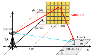
Figure 2: Simulation setup of active RIS-assisted multiuser MISO communication system.

In particular, Problem (88) can be equivalently transformed into

$$\mathop{\min}\limits_{{\varphi_{m}}}~{}~{}~{} \cos\left({-{\varphi_{m}}+\angle{b_{m}}}\right)$$ (89a)

$${\rm{s}}{\rm{.t}}{\rm{.}}~{}~{}~{} {\varphi_{m}}\in\left[{0,2\pi}\right].$$ (89b)

For a given $b_{m}$, the globally optimal solution can be obtained as

$${\varphi_{m}}=\angle{b_{m}}-\pi.$$ (90)

Correspondingly, $\theta_{m}$ is obtained as

$${\theta_{m}}={e^{j\left({\angle{b_{m}}-\pi}\right)}}.$$ (91)

Next, we consider Problem (88b). With the obtained solution of $\theta_{m}$, the value of (89a) is calculated as $-1$ and consequently, ${\mathop{\rm Re}\nolimits}\left\{{{b_{m}}\theta_{m}^{*}{a_{m}}}\right\}$ can be calculated as $-\left|{{b_{m}}}\right|{a_{m}}$. Therefore, the solution of the unconstrained Problem (88b) can be found by the following closed-form expression

$${a_{m}}=\frac{\left|{{b_{m}}}\right|}{{2\left({{{\tilde{z}}_{m,m}}+\eta{{\mathord{\buildrel{\lower 3.0pt\hbox{$\scriptscriptstyle\frown$}}\over{z}}}_{m,m}}}\right)}}.$$ (92)

The detailed procedure of the proposed element-wise ASO algorithm for solving Problem (85) is shown in Algorithm 5. It can be proved that Algorithm 5 converges as elaborated in [53].

Based on the above discussion, the proposed BCD-ASO algorithm to solve Problem (28) is presented in Algorithm 6.

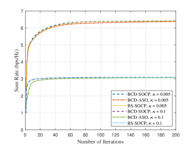
Figure 3: Convergence behaviour of the proposed algorithms.

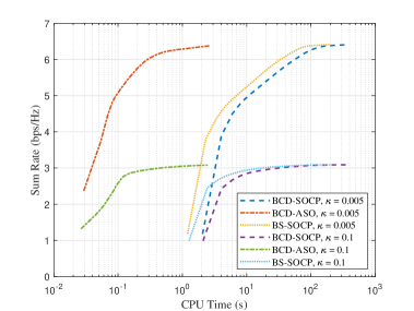
Figure 4: CPU time of the proposed algorithms.

V Simulation Results

In this section, representative simulation results are provided to validate the benefits of employing an active RIS for improving the performance of the considered multiuser MISO communication system in the presence of HWIs. The performance of the designed algorithms is evaluated as well.

V-A Simulation Setup

Consider a three-dimensional (3D) coordinate setup as depicted in Fig. 2, in which the BS and the active RIS are situated at $(0,0,10)$ and $(80,10,10)$ in meters, respectively. All users are randomly distributed within a disk centered at $(100,0,1.5)$. All the channels follow a Rician distribution. Unless otherwise specified, the simulation parameters are set as follows: the number of RIS elements $M=16$, the number of BS transmit antennas $N=4$, the number of users $K=3$, the T-HWI coefficients $\kappa_{t}=\kappa_{r}=\kappa=0.01^{2}$, the amplifier power coefficients ${\xi_{T}}={\xi_{A}}=1.2$, the circuit dissipated power at BS $P_{\rm{BS}}=9$ dBW [17], the power budget $P=20$ dBm.

V-B Baseline Schemes

Algorithm 1 in Section III is denoted as BCD-SOCP and Algorithm 6 in Section IV is denoted as BCD-ASO. In this section, the simulations are performed for comparing the performance of the developed algorithms with six baseline schemes as follows:

• BS-SOCP: We design a benchmark algorithm, where the BS beamforming matrix is designed by bisection search method in Algorithm 4 and the reflection coefficients of the active RIS are obtained by Algorithm 1.

• Active RIS [23]:  In the same scenario as considered in this paper, the algorithm proposed in [23] is adopted to jointly optimize the beamforming of the BS and the reflection coefficients of the active RIS.

• Active RandPhase: The phase shifts of the active RIS are randomly generated from $[0,2\pi]$. The BS beamforming matrix and the amplification factors are optimized by Algorithm 4 and Algorithm 5, respectively.

• Passive RIS [15]: The traditional nearly passive RIS without amplification is considered as another benchmark. The algorithm proposed in [15] is used to jointly optimize the beamforming of the BS and the phase shifts of the passive RIS. In addition, for a fair comparison, the total power budget of the nearly passive RIS-assisted system is assumed to be the same as that of active RIS system.

• Passive RandPhase [55]:  The phase shifts of the passive RIS are randomly generated, similar to scheme 3). The weighted minimum mean square error (WMMSE) method proposed in [55] is adopted to optimize the beamforming of the BS.

• Without RIS [55]: There is no RIS to aid the transmission. The WMMSE method from [55] is used to design the beamforming of the BS. Similar to scheme 4), the total power budget keeps the same as that of the active RIS-assisted system.

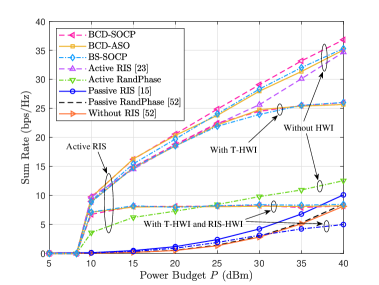
Figure 5: Sum rate versus the power budget $P$.

V-C Convergence of the Proposed Algorithms

Fig. 3 and Fig. 4 show the convergence behavior and the CPU time of various schemes while the power budget is $P=10$ dBm. Fig. 3 shows that all the schemes can reach convergence within 100 iterations, which demonstrates the effectiveness of the presented algorithms. The BCD-ASO algorithm achieves almost the same performance as the other two SOCP-based algorithms in terms of sum rate, while having a significant advantage in computational time owing to the closed-form solution. It is seen from Fig. 4 that the designed BCD-ASO algorithm has the ability to save two orders of magnitude in computational time in contrast to the BCD-SOCP algorithm and obtains a high-quality solution, which demonstrates the efficiency of the MM-based algorithm.

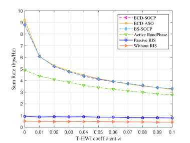
Figure 6: Sum rate versus the T-HWI coefficient $\kappa$.

V-D Impact of the Maximum Total Power Budget

Fig. 5 shows the sum rate performance versus the power budget $P$. In all schemes, the active/nearly passive RISs will not be activated until the total power budget meets the RIS circuit consumption. When the RIS is activated, the active RIS-empowered communication system outperforms the passive RIS-aided counterpart with the same total power budget and the same number of elements, owing to the fact that the elements of the active RIS possesses the ability of amplifying the incident signals. If the direct links are not too weak, deploying nearly passive RIS only brings a negligible performance gain, while the active RIS achieves a remarkable performance gain. For instance, when $P=40$ dBm and $\kappa=0$, the passive RIS realizes $23\%$ gain, while the active RIS achieves noticeable $348\%$ gain. Besides, when the sum rates of the active RIS system and passive one are equal, the total power budget required by the former is much lower, which indicates that an active RIS is promising to save the total power consumption of the communication system. Furthermore, the proposed algorithms achieve better system performance compared to the benchmark scheme proposed in [23], thereby confirming the effectiveness of our proposed methods. Moreover, the designed joint optimization algorithms obtain higher sum rates than the RandPhase scheme, verifying the advantages of the joint optimization. On the other hand, the negative impact of HWIs on the active RIS-assisted communications is more significant than that on the passive counterpart, which suggests the necessity of taking the HWIs into consideration in the active RIS design. Besides, with a high power budget $P$, the negative impact of HWIs on the performance of the active RIS-empowered communication is comparatively serious. The reason is that the distortion noise power is proportional to the signal power and that is amplified by the active RIS. Nevertheless, the performance gain brought by an active RIS is still greater than that achieved by the passive counterpart for the system with HWIs. It is also notable that the performance gain from increasing the total power budget decreases gradually, when the transceiver hardware and RIS are imperfect in an active RIS-empowered system. In other words, a specific level of total power budget exists, beyond which little sum rate gain is obtained with the increase of $P$ in the active RIS system, when the HWIs are taken into account.

V-E Impact of the HWI coefficients

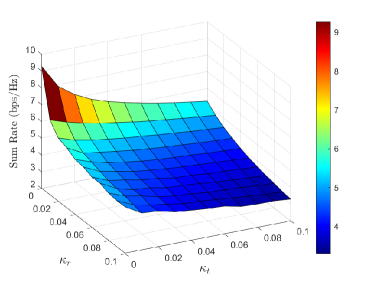
Figure 7: Sum rate versus $\kappa_{t}$ and $\kappa_{r}$ (3D).

Fig. 6 depicts the negative impact of the T-HWI coefficient $\kappa$ on the system performance. Specifically, the sum rates of different schemes deteriorate as $\kappa$ increase, due to the more prominent negative impact of HWIs. In the meantime, as $\kappa$ increases, the performance degradation of the active RIS system is more pronounced than that of the passive counterpart. For instance, when $\kappa$ increase from 0 to 0.1, the sum rate of the active RIS system decreases by 65% from 9.27 bps/Hz to 3.23 bps/Hz, while the sum rate of the nearly passive RIS system decreases by 14%. Nevertheless, the performance gain brought by the active RIS is still significantly higher than that achieved by the passive one. In other words, a more noticeable performance gain is obtained by the active RIS in contrast to the nearly passive RIS for a relatively small $\kappa$.

As illustrated in Fig. 7 and Fig. 8, we evaluate the sum rate performance as a function of the transmitter HWI coefficient $\kappa_{t}$ and the receiver HWI coefficient $\kappa_{r}$. With the increase of $\kappa_{t}$ and $\kappa_{r}$, the sum rate decreases as expected, which is consistent with the observation in Fig. 6. It can be observed that the level of hardware imperfection at the receiver poses a more severe negative impact on active RIS-empowered systems. For example, in Fig. 8, the system with $\left\{\kappa_{r}=0.01,\kappa_{t}=0\right\}$ is with the same sum rate performance as the system with $\left\{\kappa_{r}=0,\kappa_{t}=0.03\right\}$. The main reason is that the received distortion noise power is greater than the transmit distortion noise power, especially when the received signals are amplified by an active RIS.

VI Conclusion

In this work, we focused on the sum rate maximization problem in an active RIS-empowered communication system in the presence of both T-HWI and RIS-HWI. We jointly designed the transmit beamforming at the BS, along with the amplification factors and the phase shifts at the active RIS for maximizing the sum rate. To tackle the formulated non-convex optimization problem, the original problem was decoupled into more tractable subproblems. Subsequently, we developed an SOCP-based algorithm, where the optimization variables are updated alternately. To further reduce the computational complexity, we exploited the MM-based Lagrange dual decomposition method and MM-based ASO approach for deriving the closed-form solution of each subproblem. Simulation results revealed that the active RIS is a promising technique to compensate for the multiplicative fading effect. Meanwhile, the results verified the effectiveness of the designed algorithms. Compared with the systems without RIS and with nearly passive RIS, the system with active RIS achieved higher sum rate under the same total power budget, which demonstrated the superiority of the active RIS. Meanwhile, our results indicated that the performance loss caused by the HWIs were more serious in the active RIS-empowered communication system than that in the passive one, which shows the necessity of taking the HWIs into consideration in communication system design. Nevertheless, the performance gain obtained by the active RIS is still more noticeable than that achieved by the nearly passive RIS.

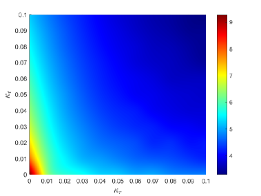
Figure 8: Sum rate versus $\kappa_{t}$ and $\kappa_{r}$ (2D).

Zhangjie Peng received the B.S. degree from Southwest Jiaotong University, Chengdu, China, in 2004, and the M.S. and Ph.D. degrees from Southeast University, Southeast University, Nanjing, China, in 2007, and 2016, respectively, all in Communication and Information Engineering. He is currently an Associate Professor at the College of Information, Mechanical and Electrical Engineering, Shanghai Normal University, Shanghai 200234, China. His research interests include reconfigurable intelligent surface (RIS), cooperative communications, information theory, physical layer security, and machine learning for wireless communications.

Zhibo Zhang received the B.S. degree from the College of Internet of Things Engineering, Hohai University, Changzhou, China, in 2020. He is currently pursuing the M.S. degree at the College of Information, Mechanical and Electrical Engineering, Shanghai Normal University, Shanghai, China. His major research interests lie in the areas of communication and signal processing, including reconfigurable intelligent surface (RIS), physical layer security and machine learning for wireless communications.

Cunhua Pan is a full professor in Southeast University.  His research interests mainly include reconfigurable intelligent surfaces (RIS), AI for Wireless, and near field communications and sensing. He has published over 170 IEEE journal papers. His papers got over 13,000 Google Scholar citations with H-index of 59. He is Clarivate Highly Cited researcher. He is/was an Editor of IEEE Transaction on Communications, IEEE Transactions on Vehicular Technology, IEEE Wireless Communication Letters, IEEE Communications Letters and IEEE ACCESS. He serves as the guest editor for IEEE Journal on Selected Areas in Communications on the special issue on xURLLC in 6G: Next Generation Ultra-Reliable and Low-Latency Communications. He also serves as a leading guest editor of IEEE Journal of Selected Topics in Signal Processing (JSTSP) Special Issue on Advanced Signal Processing for Reconfigurable Intelligent Surface-aided 6G Networks, leading guest editor of IEEE Vehicular Technology Magazine on the special issue on Backscatter and Reconfigurable Intelligent Surface Empowered Wireless Communications in 6G, leading guest editor of IEEE Open Journal of Vehicular Technology on the special issue of Reconfigurable Intelligent Surface Empowered Wireless Communications in 6G and Beyond, and leading guest editor of IEEE IEEE Transactions on Green Communications and Networking Special Issue on Design of Green Near-Field Wireless Communication Networks. He received the IEEE ComSoc Leonard G. Abraham Prize in 2022 and IEEE ComSoc Asia-Pacific Outstanding Young Researcher Award, 2022.

Marco Di Renzo (Fellow, IEEE) received the Laurea (cum laude) and Ph.D. degrees in electrical engineering from the University of L’Aquila, Italy, in 2003 and 2007, respectively, and the Habilitation ã Diriger des Recherches (Doctor of Science) degree from Université Paris-Sud (currently Paris-Saclay University), Paris, France, in 2013. He was a Fulbright Fellow with The City University of New York, USA, a Nokia Foundation Visiting Professor in Finland, and a Royal Academy of Engineering Distinguished Visiting Fellow in U.K. He is currently a CNRS Research Director (Professor) and the Head of the Intelligent Physical Communications Group, Laboratory of Signals and Systems (L2S), CNRS and CentraleSupelec, Paris-Saclay University. He is also an Elected Member of the L2S Board Council and a member of the L2S Management Committee and the Admission and Evaluation Committee of the Ph.D. School on Information and Communication Technologies, Paris-Saclay University. He is a Founding Member and the Academic Vice Chair of the Industry Specification Group (ISG) on Reconfigurable Intelligent Surfaces (RIS), European Telecommunications Standards Institute (ETSI), where he served as the Rapporteur for the work item on communication models, channel models, and evaluation methodologies. He is a fellow of IET and AAIA, an Academician of AIIA, an Ordinary Member of the European Academy of Sciences and Arts and the Academia Europaea, and a Highly Cited Researcher. He is also serving as a Voting Member for the Fellow Evaluation Standing Committee and as the Director of Journals of the IEEE Communications Society. His recent research awards include the 2021 EURASIP Best Paper Award, the 2022 IEEE COMSOC Outstanding Paper Award, the 2022 Michel Monpetit Prize conferred by the French Academy of Sciences, the 2023 EURASIP Best Paper Award, the 2023 IEEE ICC Best Paper Award, the 2023 IEEE COMSOC Fred W. Ellersick Prize, the 2023 IEEE COMSOC Heinrich Hertz Award, the 2023 IEEE VTS James Evans Avant Garde Award, and the 2023 IEEE COMSOC Technical Recognition Award from the Signal Processing and Computing for Communications Technical Committee. He holds the 2023 France-Nokia Chair of Excellence in ICT. He served as the Editor-in-Chief for IEEE COMMUNICATIONS LETTERS from 2019 to 2023. He is serving on the Advisory Board.

Octavia A. Dobre (Fellow, IEEE) is a Professor and Canada Research Chair Tier 1 with Memorial University, Canada. She was a Visiting Professor with Massachusetts Institute of Technology, USA and Université de Bretagne Occidentale, France. Her research interests encompass wireless communication and networking technologies, as well as optical and underwater communications. She has (co-)authored over 500 refereed papers in these areas. Dr. Dobre serves as the VP Publications of the IEEE Communications Society. She was the inaugural Editor-in-Chief (EiC) of the IEEE Open Journal of the Communications Society and the EiC of the IEEE Communications Letters. Dr. Dobre was a Fulbright Scholar, Royal Society Scholar, and Distinguished Lecturer of the IEEE Communications Society. She obtained Best Paper Awards at various conferences, including IEEE ICC, IEEE Globecom, IEEE WCNC, and IEEE PIMRC. Dr. Dobre is an elected member of the European Academy of Sciences and Arts, a Fellow of the Engineering Institute of Canada, and a Fellow of the Canadian Academy of Engineering.

Jiangzhou Wang (Fellow, IEEE) is a Professor with the University of Kent, U.K. He has published more than 500 papers and five books. His research focuses on mobile communications. He was a recipient of the 2022 IEEE Communications Society Leonard G. Abraham Prize. He was the Technical Program Chair of the 2019 IEEE International Conference on Communications (ICC2019), Shanghai, Executive Chair of the IEEE ICC2015, London, and Technical Program Chair of the IEEE WCNC2013. He is/was the editor of a number of international journals, including IEEE Transactions on Communications from 1998 to 2013. Professor Wang is a Foreign Member of the Chinese Academy of Engineering (CAE), a Fellow of the Royal Academy of Engineering (RAEng), U.K., Fellow of the IEEE, and Fellow of the IET.

References

• [1] W. Saad, M. Bennis, and M. Chen, “A vision of 6G wireless systems: Applications, trends, technologies, and open research problems,” IEEE Netw., vol. 34, no. 3, pp. 134–142, May/Jun. 2020.
• [2] C. Pan et al., “Reconfigurable intelligent surfaces for 6G systems: Principles, applications, and research directions,” IEEE Commun. Mag., vol. 59, no. 6, pp. 14–20, Jun. 2021.
• [3] C. Huang, S. Hu, G. C. Alexandropoulos, A. Zappone, C. Yuen, R. Zhang, M. Di Renzo, and M. Debbah, “Holographic MIMO surfaces for 6G wireless networks: Opportunities, challenges, and trends,” IEEE Wireless Commun., vol. 27, no. 5, pp. 118–125, Oct. 2020.
• [4] C. Pan et al., “An overview of signal processing techniques for RIS/IRS-aided wireless systems,” IEEE J. Sel. Topics Signal Process., vol. 16, no. 5, pp. 883–917, Aug. 2022.
• [5] Q. Wu and R. Zhang, “Towards smart and reconfigurable environment: Intelligent reflecting surface aided wireless network,” IEEE Commun. Mag., vol. 58, no. 1, pp. 106–112, Jan. 2020.
• [6] Y. Liu, X. Liu, X. Mu, T. Hou, J. Xu, M. Di Renzo, and N. Al-Dhahir, “Reconfigurable intelligent surfaces: Principles and opportunities,” IEEE Commun. Surv. Tut., vol. 23, no. 3, pp. 1546–1577, Jul.-Sep. 2021.
• [7] M. Di Renzo, A. Zappone, M. Debbah, M.-S. Alouini, C. Yuen, J. de Rosny, and S. Tretyakov, “Smart radio environments empowered by reconfigurable intelligent surfaces: How it works, state of research, and the road ahead,” IEEE J. Sel. Areas Commun., vol. 38, no. 11, pp. 2450–2525, Nov. 2020.
• [8] W. Tang, M. Z. Chen, J. Y. Dai, Y. Zeng, X. Zhao, S. Jin, Q. Cheng, and T. Cui, “Wireless communications with programmable metasurface: New paradigms, opportunities, and challenges on transceiver design,” IEEE Wireless Commun., vol. 27, no. 2, pp. 180–187, Apr. 2020.
• [9] C. Pan, H. Ren, K. Wang, M. Elkashlan, A. Nallanathan, J. Wang, and L. Hanzo, “Intelligent reflecting surface aided MIMO broadcasting for simultaneous wireless information and power transfer,” IEEE J. Sel. Areas Commun., vol. 38, no. 8, pp. 1719–1734, Aug. 2020.
• [10] T. Bai, C. Pan, Y. Deng, M. Elkashlan, A. Nallanathan, and L. Hanzo, “Latency minimization for intelligent reflecting surface aided mobile edge computing,” IEEE J. Sel. Areas Commun., vol. 38, no. 11, pp. 2666–2682, Nov. 2020.
• [11] L. Zhang, Y. Wang, W. Tao, Z. Jia, T. Song, and C. Pan, “Intelligent reflecting surface aided MIMO cognitive radio systems,” IEEE Trans. Veh. Technol., vol. 69, no. 10, pp. 11 445–11 457, Oct. 2020.
• [12] S. Hong, C. Pan, H. Ren, K. Wang, and A. Nallanathan, “Artificial-noise-aided secure MIMO wireless communications via intelligent reflecting surface,” IEEE Trans. Commun., vol. 68, no. 12, pp. 7851–7866, Dec. 2020.
• [13] A. R. Ndjiongue, T. M. N. Ngatched, O. A. Dobre, and H. Haas, “Toward the use of re-configurable intelligent surfaces in VLC systems: Beam steering,” IEEE Wireless Commun., vol. 28, no. 3, pp. 156–162, Jun. 2021.
• [14] Y. Pan, K. Wang, C. Pan, H. Zhu, and J. Wang, “UAV-assisted and intelligent reflecting surfaces-supported terahertz communications,” IEEE Wireless Commun. Lett., vol. 10, no. 6, pp. 1256–1260, Jun. 2021.
• [15] C. Pan et al., “Multicell MIMO communications relying on intelligent reflecting surfaces,” IEEE Trans. Wireless Commun., vol. 19, no. 8, pp. 5218–5233, May 2020.
• [16] Z. Peng, Z. Zhang, C. Pan, L. Li, and A. L. Swindlehurst, “Multiuser full-duplex two-way communications via intelligent reflecting surface,” IEEE Trans. Signal Process., vol. 69, pp. 837–851, Jan. 2021.
• [17] C. Huang, A. Zappone, G. C. Alexandropoulos, M. Debbah, and C. Yuen, “Reconfigurable intelligent surfaces for energy efficiency in wireless communication,” IEEE Trans. Wireless Commun., vol. 18, no. 8, pp. 4157–4170, Aug. 2019.
• [18] Q. Wu and R. Zhang, “Intelligent reflecting surface enhanced wireless network via joint active and passive beamforming,” IEEE Trans. Wireless Commun., vol. 18, no. 11, pp. 5394–5409, Nov. 2019.
• [19] G. Zhou, C. Pan, H. Ren, K. Wang, and A. Nallanathan, “A framework of robust transmission design for IRS-aided MISO communications with imperfect cascaded channels,” IEEE Trans. Signal Process., vol. 68, pp. 5092–5106, Aug. 2020.
• [20] L. Yang, Y. Yang, D. B. d. Costa, and I. Trigui, “Outage probability and capacity scaling law of multiple RIS-aided networks,” IEEE Wireless Commun. Lett., vol. 10, no. 2, pp. 256–260, Feb. 2021.
• [21] M. Najafi, V. Jamali, R. Schober, and H. V. Poor, “Physics-based modeling and scalable optimization of large intelligent reflecting surfaces,” IEEE Trans. Commun., vol. 69, no. 4, pp. 2673–2691, Apr. 2021.
• [22] Z.-Q. He and X. Yuan, “Cascaded channel estimation for large intelligent metasurface assisted massive MIMO,” IEEE Wireless Commun. Lett., vol. 9, no. 2, pp. 210–214, Feb, 2020.
• [23] Z. Zhang, L. Dai, X. Chen, C. Liu, F. Yang, R. Schober, and H. V. Poor, “Active RIS vs. passive RIS: Which will prevail in 6G?” IEEE Trans. Commun., vol. 71, no. 3, pp. 1707–1725, Mar. 2023.
• [24] R. Long, Y.-C. Liang, Y. Pei, and E. G. Larsson, “Active reconfigurable intelligent surface-aided wireless communications,” IEEE Trans. Wireless Commun., vol. 20, no. 8, pp. 4962–4975, Aug. 2021.
• [25] K. Zhi, C. Pan, H. Ren, K. K. Chai, and M. Elkashlan, “Active RIS versus passive RIS: Which is superior with the same power budget?” IEEE Commun. Lett., vol. 26, no. 5, pp. 1150–1154, May 2022.
• [26] A. R. Ndjiongue, T. M. N. Ngatched, O. A. Dobre, and H. Haas, “Design of a power amplifying-RIS for free-space optical communication systems,” IEEE Wireless Commun., vol. 28, no. 6, pp. 152–159, Dec. 2021.
• [27] C. You and R. Zhang, “Wireless communication aided by intelligent reflecting surface: Active or passive?” IEEE Wireless Commun. Lett., vol. 10, no. 12, pp. 2659–2663, Dec. 2021.
• [28] D. Xu, X. Yu, D. W. Kwan Ng, and R. Schober, “Resource allocation for active IRS-assisted multiuser communication systems,” in Proc. 55th Asilomar Conf. Signals, Syst. Comput., pp. 113–119, Otc. 2021.
• [29] R. K. Fotock, A. Zappone, and M. Di Renzo, “Energy efficiency in RIS-aided wireless networks: Active or passive RIS?” 2023. [Online]. Available: https://arxiv.org/abs/2303.04505
• [30] Y. Ma, M. Li, Y. Liu, Q. Wu, and Q. Liu, “Active reconfigurable intelligent surface for energy efficiency in MU-MISO systems,” IEEE Trans. Veh. Technol., vol. 72, no. 3, pp. 4103–4107, Mar. 2023.
• [31] L. Dong, H.-M. Wang, and J. Bai, “Active reconfigurable intelligent surface aided secure transmission,” IEEE Trans. Veh. Technol., vol. 71, no. 2, pp. 2181–2186, Feb. 2022.
• [32] Z. Peng, R. Weng, Z. Zhang, C. Pan, and J. Wang, “Active reconfigurable intelligent surface for mobile edge computing,” IEEE Wireless Commun. Lett., vol. 11, no. 12, pp. 2482–2486, Dec. 2022.
• [33] Y. Gao, Q. Wu, G. Zhang, W. Chen, D. W. K. Ng, and M. Di Renzo, “Beamforming optimization for active intelligent reflecting surface-aided SWIPT,” IEEE Trans. Wireless Commun., vol. 22, no. 1, pp. 362–378, Jan. 2023.
• [34] E. Björnson, J. Hoydis, M. Kountouris, and M. Debbah, “Massive MIMO systems with non-ideal hardware: Energy efficiency, estimation, and capacity limits,” IEEE Trans. Inf. Theory, vol. 60, no. 11, pp. 7112–7139, Nov. 2014.
• [35] Z. Peng, Z. Zhang, L. Kong, C. Pan, L. Li, and J. Wang, “Deep reinforcement learning for RIS-aided multiuser full-duplex secure communications with hardware impairments,” IEEE Internet Things J., vol. 9, no. 21, pp. 21 121–21 135, Nov. 2022.
• [36] A. A. Boulogeorgos and A. Alexiou, “How much do hardware imperfections affect the performance of reconfigurable intelligent surface-assisted systems?” IEEE Open J. Commun. Soc.S, vol. 1, pp. 1185–1195, Aug. 2020.
• [37] H. Shen, W. Xu, S. Gong, C. Zhao, and D. W. K. Ng, “Beamforming optimization for IRS-aided communications with transceiver hardware impairments,” IEEE Trans. Commun., vol. 69, no. 2, pp. 1214–1227, Feb. 2021.
• [38] Z. Peng, Z. Chen, C. Pan, G. Zhou, and H. Ren, “Robust transmission design for RIS-aided communications with both transceiver hardware impairments and imperfect CSI,” IEEE Wireless Commun. Lett., vol. 11, no. 3, pp. 528–532, Mar. 2022.
• [39] Z. Xing, R. Wang, J. Wu, and E. Liu, “Achievable rate analysis and phase shift optimization on intelligent reflecting surface with hardware impairments,” IEEE Trans. Wireless Commun., vol. 20, no. 9, pp. 5514–5530, Sep. 2021.
• [40] G. Zhou, C. Pan, H. Ren, K. Wang, and Z. Peng, “Secure wireless communication in RIS-aided MISO system with hardware impairments,” IEEE Wireless Commun. Lett., vol. 10, no. 6, pp. 1309–1313, Jun. 2021.
• [41] Z. Chu, J. Zhong, P. Xiao, D. Mi, W. Hao, R. Tafazolli, and A. P. Feresidis, “RIS assisted wireless powered IoT networks with phase shift error and transceiver hardware impairment,” IEEE Trans. Commun., vol. 70, no. 7, pp. 4910–4924, Jul. 2022.
• [42] Z. Peng, X. Liu, C. Pan, L. Li, and J. Wang, “Multi-pair D2D communications aided by an active RIS over spatially correlated channels with phase noise,” IEEE Wireless Commun. Lett., vol. 11, no. 10, pp. 2090–2094, Oct. 2022.
• [43] Q. Li, M. El-Hajjar, I. Hemadeh, D. Jagyasi, A. Shojaeifard, and L. Hanzo, “Performance analysis of active RIS-aided systems in the face of imperfect CSI and phase shift noise,” IEEE Trans. Veh. Technol., vol. 72, no. 6, pp. 8140–8145, Jun. 2023.
• [44] C. Hu, L. Dai, S. Han, and X. Wang, “Two-timescale channel estimation for reconfigurable intelligent surface aided wireless communications,” IEEE Trans. Commun., vol. 69, no. 11, pp. 7736–7747, Nov. 2021.
• [45] L. Wei, C. Huang, G. C. Alexandropoulos, C. Yuen, Z. Zhang, and M. Debbah, “Channel estimation for RIS-empowered multi-user MISO wireless communications,” IEEE Trans. Commun., vol. 69, no. 6, pp. 4144–4157, Jun. 2021.
• [46] H. Chen, N. Li, R. Long, and Y.-C. Liang, “Channel estimation and training design for active RIS aided wireless communications,” IEEE Wireless Commun. Lett., Jul. 2023, early access, doi: 10.1109/LWC.2023.3297231.
• [47] J.-F. Bousquet, S. Magierowski, and G. G. Messier, “A 4-GHz active scatterer in 130-nm CMOS for phase sweep amplify-and-forward,” IEEE Trans. Circuits Syst. I, vol. 59, no. 3, pp. 529–540, Mar. 2012.
• [48] Q. Zhang, S. Jin, K.-K. Wong, H. Zhu, and M. Matthaiou, “Power scaling of uplink massive MIMO systems with arbitrary-rank channel means,” IEEE J. Sel. Topics Signal Process., vol. 8, no. 5, pp. 966–981, Oct. 2014.
• [49] Z. Peng, R. Weng, C. Pan, G. Zhou, M. Di Renzo, and A. Lee Swindlehurst, “Robust transmission design for RIS-assisted secure multiuser communication systems in the presence of hardware impairments,” IEEE Trans. Wireless Commun., Mar. 2023, early access, doi: 10.1109/TWC.2023.3252046.
• [50] J. Wang, S. Gong, Q. Wu, and S. Ma, “RIS-aided MIMO systems with hardware impairments: Robust beamforming design and analysis,” IEEE Trans. Wireless Commun., Feb. 2023, early access, doi: 10.1109/TWC.2023.3246990.
• [51] K. Shen and W. Yu, “Fractional programming for communication systems—part I: Power control and beamforming,” IEEE Trans. Signal Process., vol. 66, no. 10, pp. 2616–2630, May 2018.
• [52] M. Grant and S. Boyd., “CVX: MATLAB Software for Disciplined Convex Programming, Version 2.1.” Mar. 2014. [Online]. Available: https://cvxr.com/cvx
• [53] G. Cui, X. Yu, G. Foglia, Y. Huang, and J. Li, “Quadratic optimization with similarity constraint for unimodular sequence synthesis,” IEEE Trans. Signal Process., vol. 65, no. 18, pp. 4756–4769, Sep. 2017.
• [54] S. Boyd and L. Vandenberghe, Convex optimization.   Cambridge, U.K.: Cambridge Univ. Press, 2004.
• [55] Q. Shi, M. Razaviyayn, Z.-Q. Luo, and C. He, “An iteratively weighted MMSE approach to distributed sum-utility maximization for a MIMO interfering broadcast channel,” IEEE Trans. Signal Process., vol. 59, no. 9, pp. 4331–4340, Sep. 2011.