Uncertainty, Calibration, and Membership Inference Attacks: An Information-Theoretic Perspective

Abstract

In a membership inference attack (MIA), an attacker exploits the overconfidence exhibited by typical machine learning models to determine whether a specific data point was used to train a target model. In this paper, we analyze the performance of the state-of-the-art likelihood ratio attack (LiRA) within an information-theoretical framework that allows the investigation of the impact of the aleatoric uncertainty in the true data generation process, of the epistemic uncertainty caused by a limited training data set, and of the calibration level of the target model. We compare three different settings, in which the attacker receives decreasingly informative feedback from the target model: confidence vector (CV) disclosure, in which the output probability vector is released; true label confidence (TLC) disclosure, in which only the probability assigned to the true label is made available by the model; and decision set (DS) disclosure, in which an adaptive prediction set is produced as in conformal prediction. We derive bounds on the advantage of an MIA adversary with the aim of offering insights into the impact of uncertainty and calibration on the effectiveness of MIAs. Simulation results demonstrate that the derived analytical bounds predict well the effectiveness of MIAs.

I Introduction

I-A Context and Motivation

By attempting to infer whether individual data records were used to train a machine learning model, membership inference attacks (MIAs) pose a significant privacy risk, particularly in sensitive domains such as healthcare or recommendation systems, revealing personal information without consent [1, 2]. Analyzing MIAs is crucial to understanding privacy threats to machine learning models, as well as to developing robust countermeasures [3, 4, 5].

Machine learning models that exhibit overconfidence in predictions are known to be more susceptible to MIAs [1, 2, 5]. In fact, by assigning disproportionately high confidence scores to predictions on inputs present in the training set, overconfident models inadvertently leak information about their training data. This leakage enables attackers to infer the presence of specific data points in the training data set with greater accuracy, thereby compromising data privacy. Improving the calibration, i.e., the uncertainty quantification capabilities, of predictive models is thus a common step to safeguard against MIAs [5].

However, the vulnerability to MIAs is not solely contingent upon model calibration. In fact, models with the same calibration level may exhibit significantly different susceptibilities to MIAs depending on the underlying predictive uncertainty level. Predictive uncertainty can be broadly classified into aleatoric uncertainty and epistemic uncertainty [6, 7]. Aleatoric uncertainty reflects the inherent unpredictability of the data generation process; while epistemic uncertainty reflects limitations in the knowledge of the model caused by access to limited training data. As the predictive uncertainty increases, due to either aleatoric uncertainty or epistemic uncertainty, a model with a fixed calibration level would tend to produce more balanced confidence levels, making it more difficult to carry out a successful MIA.

Furthermore, for a black-box attacker, epistemic uncertainty creates the additional complication of increasing the uncertainty about the actual model parameters of the target model. In fact, the variability in the model parameter space associated with an unknown training data set increases with smaller data set sizes, since larger data sets tend to all yield models that minimize the underlying population loss.

Overall, exploring the impact and interplay of uncertainty and calibration is essential for a comprehensive understanding of MIAs, supporting the development of more effective privacy-preserving strategies.

I-B State of the Art

Confidence vector (CV) disclosure: The key reference [1] introduced MIAs by focusing on black-box scenarios in which the attacker can query the target model once for the given input of interest, obtaining the full confidence vector (CV) produced at the output of the model. The authors turned the MIA into a classification problem, and trained a neural network to distinguish between the target model’s responses to data points inside and outside the training set. To this end, the authors proposed to construct shadow models that are designed to imitate the behavior of the target model for inputs inside and outside the training set. Using the shadow models, a neural network is trained to distinguish the two types of inputs. Follow-up work includes [8], which relaxed the assumptions on the knowledge of data distribution and model architecture by leveraging an ensemble of basic classification networks. Attacks based on the evaluation of the entropy of the confidence probability vectors were studied in [3, 9].

True label confidence (TLC) disclosure: Based on the observation that overconfident models tend to generate higher confidence scores to the true label when queried on training data than on unseen test data [5], various studies explored settings in which the target model returns only the true label confidence (TLC) level, or equivalently the corresponding prediction loss [8, 3, 10, 11]. In such scenarios, the attacker sets a threshold on the target model’s confidence assigned to the true label to identify the training data points [3, 9]. To optimize the threshold, one can aim at maximizing the true positive rate (TPR) with a constraint on a maximum false positive rate (FPR) [10, 12].

Reference [2] introduced the likelihood ratio attack (LiRA), in which Gaussian distributions are fit to the TLC generated by shadow models trained to imitate models trained with and without the candidate data point. LiRA is then conducted through a parametric likelihood ratio test. Reference [13] improved LiRA by adding adversarial noise to the input to amplify the output gap between the two classes of shadow models (see also [14]).

Label-only and decision set (DS) disclosure: As another disclosure model, other studies have developed label-only attacks, for which the attacker has access solely to predicted labels. Reference [3] proposed to identify samples that are correctly classified as part of the training data sets [5]. Further research exploited the fact that the predicted labels of overconfident models are less sensitive to perturbations on inputs derived from training data as compared to previously unseen data. By analyzing the variability of predicted labels in the presence of adversarial perturbations [15] or data augmentations [16], attackers can thus attempt to identify training data points.

In this paper, we generalize label-only disclosure to inference settings in which the target model generates a decision set (DS), i.e., a subset of labels, as its prediction output. Decision sets are typically generated by including all the labels whose confidence is above a threshold. A DS provides information about the uncertainty of the prediction through its size, and it can be derived using formal methods such as conformal prediction [17, 18, 19].

Theoretical analysis of membership inference attacks: Numerous studies have explored the link between model calibration and privacy risks via experiments [1, 2, 5] or via scenario-specific theoretical analyses [3, 4, 10, 20, 21]. Notably, a line of work is motivated by the opposite nature of the goal of MIAs – revealing a training data point – and of differential privacy (DP) mechanisms – obscuring the presence or absence of a training data point [22]. Based on this observation, upper bounds on the attacker’s advantage [3, 4] and positive predictive value [10] were studied for DP-protected models. These works focus on the theoretical relationship between the DP metrics and MIA success measures. Furthermore, reference [20] established universal bounds on the success rate of MIAs as a function of the target model’s generalization gap, while assuming a white-box attacker. Finally, results that target symmetric and redundancy-invariant algorithms were presented in [21].

I-C Contributions and Organization

In this paper, we introduce a unified theoretical framework to analyze the performance of MIA under CV, TLC, and DS disclosures, while assuming black-box attacks as in [2, 1] and focusing on the impact and interplay of calibration and predictive uncertainty. The main contributions of this paper are summarized as follows.

• As illustrated in Fig. 1, treating MIA design for black-box models as a hypothesis-testing problem, we introduce a general information-theoretical framework to analyze the attacker’s advantage for CV, TLC, and DS disclosure settings. Specifically, as seen in Fig. 2, the proposed methodology addresses LiRA-style attacks built from shadow models that imitate the behavior of the target model to inputs inside and outside the training set.

• The proposed framework models the confidence probability vectors produced by the shadow models using Dirichlet distributions with the aim of accounting for both aleatoric uncertainty – the inherent randomness in the data-generation process – and epistemic uncertainty – quantifying the variability of the shadow models as a function of the unknown training set. Under this working assumption, information-theoretic upper bounds on the attacker’s advantage under CV, TLC, and DS observations are derived that enable a theoretical investigation of the effectiveness of MIA as a function of the model’s calibration, as well as of the aleatoric and epistemic uncertainties.

• Simulation results validate the analysis, providing insights into the influence of calibration and predictive uncertainty on the attacker’s advantage under CV, TLC, and DS disclosure settings.

The remainder of this paper is organized as follows. In Sec. II, we outline the problem, review the LiRA framework, and introduce relevant performance metrics. Sec. III reviews a performance bound for MIA, and defines aleatoric uncertainty and calibration. In Sec. IV, we analyze the performance of MIA given CV, TLC, and DS observations. Sec. V empirically evaluates the performance of MIA, validating our theoretical findings. Sec. VI concludes the paper.

II Problem Definition

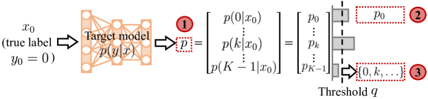
Figure 1: Membership inference attack (MIA): An attacker queries an unknown target $K$-class classification model with some input $x_{0}$ whose true label, known to the attacker, is $y_{0}=0$ in order to determine whether data point $(x_{0},y_{0})$ was used in the training of the model. The attacker receives from the model one of the following: \scriptsize{1}⃝ the confidence vector (CV) $p$; \scriptsize{2}⃝ the true label confidence (TLC) $p_{0}=p(0|x_{0})$; or \scriptsize{3}⃝ the decision set (DS) $O(p)$ consisting of all labels $k$ with confidence level $p(k|x_{0})$ no smaller than a threshold $q$.

A membership inference attack (MIA) aims at determining whether a specific example $(x_{0},y_{0})$ was used in the training of a target model [1]. In line with prior studies [1, 2, 14, 8], the adversary is assumed to know: (i) the underlying data distribution, e.g., in the form of a related data set; (ii) the target model architecture; and (iii) the training algorithm used to design the target model. However, the attacker does not have access to the trained model parameters, and, as shown in Fig. 1, it can only query the target model once, at attack time, by feeding it input $x_{0}$. As a result of this query, the target model returns one of the following types of information: \small{1}⃝ the entire output confidence vector [1]; \small{2}⃝ the true label confidence probability [2]; \small{3}⃝ a prediction set containing the set of labels with confidence levels no smaller than a known threshold [18].

II-A Membership Inference Attack as Hypothesis Testing

Focusing on a $K$-class classification problem, the target model $p(y|x,\theta)$ is a conditional probability distribution over the label variable $y\in\left\{0,1,\ldots,K-1\right\}$ given input $x$ that is parameterized by a vector $\theta$. The model parameter vector $\theta$ is optimized by the target model on the basis of a training algorithm

$$\theta_{\mathcal{D}^{\mathrm{tr}}}=\mathcal{T}(\mathcal{D}^{\mathrm{tr}}),$$ (1)

mapping a training data set $\mathcal{D}^{\mathrm{tr}}$ to a model parameter vector $\theta_{\mathcal{D}^{\mathrm{tr}}}$. The training data set $\mathcal{D}^{\mathrm{tr}}$ consists of pairs $(x,y)$ generated from the ground-truth distribution $p^{*}(x,y)$.

As mentioned in [2], we assume that the attacker knows the data generation distribution $p^{*}(x,y)$, as well as the training algorithm $\mathcal{T}(\cdot)$ in (1). However, it does not have access to the training data set $\mathcal{D}^{\mathrm{tr}}$ and to the trained parameter vector $\theta_{\mathcal{D}^{\mathrm{tr}}}$. Furthermore, the attacker can query once the target model with input $x_{0}$ of interest.

The information released by the target model is a function of the confidence probability vector $p(y|x_{0},\theta_{\mathcal{D}^{\mathrm{tr}}})$ output by the model in response to a query with input $x_{0}$. We write the confidence probability vector as

$$p=\begin{bmatrix}p_{0}\\ \vdots\\ p_{K-1}\end{bmatrix}=\begin{bmatrix}p(y=0|x_{0})\\ \vdots\\ p(y=K-1|x_{0})\end{bmatrix}$$ (2)

with $p_{k}\in[0,1]$ and $\sum_{k=0}^{K-1}p_{k}=1$. Without loss of generality, we reorder the entries so that the first element, $p_{0}$, corresponds to the probability assigned by the model to the true label $y_{0}$. As illustrated in Fig. 1, we consider the following three different query outputs: \small{1}⃝ confidence vector (CV), which produces the entire vector (2) as its output, i.e.,

$$O(p)=p;$$ (3)

\small{2}⃝ true label confidence (TLC), which only returns the confidence of the true label, i.e.,

$$O(p)=p_{0};$$ (4)

\small{3}⃝ decision set (DS), which generates a set of labels whose corresponding confidence levels are no smaller than a given threshold $q$.

$$O(p)=\mathds{1}(p\geq q),$$ (5)

where $\mathds{1}(\cdot)$ is the indicator function and the threshold $q$ is known to the attacker.

A CV observation (3) provides the attacker with the most information about the model, and it can thus be considered as the worst-case setting for the model vis-à-vis the attacker [1]. The model may, however, only release the confidence level for the chosen label $y_{0}=0$, as studied in [2]. The resulting TLC output (4) generally results in less effective attacks as compared to CV observations. Finally, a DS output (5) is common for models designed for reliable decision-making using tools such as conformal prediction [17]. An attack based on (5) may be considered as a form of label-only attack [16], which has not been explicitly studied in the literature.

Based on the available information on distribution $p^{*}(x,y)$, training algorithm $\mathcal{T}(\cdot)$, and output $O(p)$ of the model (3), (4), or (5), in LiRA, the attacker aims at distinguishing two hypotheses

$$\mathcal{H}^{\mathrm{out}}:(x_{0},y_{0})\notin\mathcal{D}^{\mathrm{tr}},$$ (6a)

$$\mathcal{H}^{\mathrm{in}}:(x_{0},y_{0})\in\mathcal{D}^{\mathrm{tr}}.$$ (6b)

Accordingly, the null hypothesis $\mathcal{H}^{\mathrm{out}}$ posits that the target model $p(y|x,\theta_{\mathcal{D}^{\mathrm{tr}}})$ is trained on a data set $\mathcal{D}^{\mathrm{tr}}$ that does not include the target example $(x_{0},y_{0})$, while the alternative hypothesis $\mathcal{H}^{\mathrm{in}}$ asserts the opposite.

II-B Likelihood Ratio Attack

Based on the observation $O=O(p)$, the attacker computes a test function $T(O)$, and then it decides for either hypothesis according to the rule

$$\mathrm{if} ~{}T(O)=0,~{}\mathrm{choose}~{}\mathcal{H}^{\mathrm{out}},$$ (7a)

$$\mathrm{else~{}if} ~{}T(O)=1,~{}\mathrm{choose}~{}\mathcal{H}^{\mathrm{in}}.$$ (7b)

In order to construct the test variable $T(O)$, in this paper, we focus on the state-of-the-art likelihood ratio attack (LiRA). As illustrated in Fig. 2, LiRA estimates the distributions $f^{\mathrm{out}}(O)$ and $f^{\mathrm{in}}(O)$ of the observation $O$ during a preliminary offline phase. It is emphasized that the original LiRA focused solely on TLC outputs (4), and assumed Gaussian distributions $f^{\mathrm{out}}(O)$ and $f^{\mathrm{in}}(O)$ to obtain a practical algorithm. In this paper, we study a more general framework, allowing for any of the outputs $O$ in (3)–(5), with the aim of deriving analytical insights.

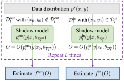
Figure 2: Illustration of the estimation process of the distribution $f^{\mathrm{out}}(O)$ of the observation $O$ under the assumption $\mathcal{H}^{\mathrm{out}}$ that the training data does not include $(x_{0},y_{0})$ and of the distribution $f^{\mathrm{in}}(O)$ under the assumption $\mathcal{H}^{\mathrm{in}}$ that the target model is trained using the pair $(x_{0},y_{0})$.

Using the available information about the distribution $p^{*}(x,y)$, training algorithm $\mathcal{T}(\cdot)$, and model architecture $p(y|x,\theta)$, in LiRA, the attacker constructs $L$ independent pairs of shadow models, with each shadow model sharing the same architecture and training algorithm as the target model. To train each model pair $l=1,2,\ldots,L$, the attacker generates two data sets. The first data set, $\mathcal{D}_{l}^{\mathrm{out}}$, contains $N^{\mathrm{tr}}$ examples sampled i.i.d. from the data distribution $p^{*}(x,y)$; while the second data set, $\mathcal{D}_{l}^{\mathrm{in}}$, contains $N^{\mathrm{tr}}-1$ examples sampled i.i.d. from $p^{*}(x,y)$ as well as the target input-output pair $(x_{0},y_{0})$:

$$\mathcal{D}^{\mathrm{out}}_{l}=\left\{(x_{n},y_{n})\right\}_{n=1}^{N^{\mathrm{tr}}}~{}\mathrm{with}~{}(x_{n},y_{n})\sim p^{*}(x,y)$$ (8a)

$$\mathcal{D}^{\mathrm{in}}_{l}=\left\{(x_{0},y_{0})\right\}\cup\left\{(x_{n},y_{n})\right\}_{n=2}^{N^{\mathrm{tr}}}~{}\mathrm{with}~{}(x_{n},y_{n})\sim p^{*}(x,y)$$ (8b)

In practice, the sets (8a)–(8b) can be obtained using data related to the training data set.

As illustrated in Fig. 2, using the data sets $\mathcal{D}_{l}^{\mathrm{out}}$ and $\mathcal{D}_{l}^{\mathrm{in}}$ and the known training algorithm $\mathcal{T}(\cdot)$, the attacker trains two models as

$$\theta_{\mathcal{D}_{l}^{\mathrm{out}}}=\mathcal{T}(\mathcal{D}_{l}^{\mathrm{out}})~{}\mathrm{and}~{}\theta_{\mathcal{D}_{l}^{\mathrm{in}}}=\mathcal{T}(\mathcal{D}_{l}^{\mathrm{in}})$$ (9)

for all $l=1,2,\ldots,L$. Using the $L$ models $\{p(y|x,\theta_{\mathcal{D}_{l}^{\mathrm{out}}})\}_{l=1}^{L}$, the attacker estimates the distribution $f^{\mathrm{out}}(O)$ of the outputs $O$ in (3)–(5) under the hypothesis $\mathcal{H}^{\mathrm{out}}$; while distribution $f^{\mathrm{in}}(O)$ of the outputs $O$ under the hypothesis $\mathcal{H}^{\mathrm{in}}$ is similarly estimated from the $L$ models $\{p(y|x,\theta_{\mathcal{D}_{l}^{\mathrm{in}}})\}_{l=1}^{L}$.

Distributions $f^{\mathrm{out}}(O)$ and $f^{\mathrm{in}}(O)$ represent the probability density functions of the observations $O$ under the hypotheses $\mathcal{H}^{\mathrm{out}}$ and $\mathcal{H}^{\mathrm{in}}$, respectively. Accordingly, the randomness captured by the distributions $f^{\mathrm{out}}(O)$ and $f^{\mathrm{in}}(O)$ reflects the inherent uncertainty of the attacker about the training data set $\mathcal{D}^{\mathrm{tr}}$ used to optimize the target model as per (1). For the analysis in what follows, we assume $L$ to be large enough that distributions $f^{\mathrm{out}}(O)$ and $f^{\mathrm{in}}(O)$ are correctly estimated by the attacker. This assumption represents a meaningful worst-case condition for the target model, since $L$ is only limited by the computational complexity of the attacker.

Once the distributions $f^{\mathrm{out}}(O)$ and $f^{\mathrm{in}}(O)$ are estimated for the given pair $(x_{0},y_{0})$ of interest, LiRA applies a likelihood ratio test to the output $O$ produced by the target model in response to input $x_{0}$. Accordingly, the decision variable used in the decision (7) is given by

$$T(O)=\mathds{1}\Big{(}\log\Big{(}\frac{f^{\mathrm{out}}(O)}{f^{\mathrm{in}}(O)}\Big{)}<\tau\Big{)}$$ (10)

for some threshold $\tau\geq 0$.

II-C Performance Metrics

The effectiveness of the test (10), and hence of the LiRA, is gauged by the type-I error $1-\alpha$ and the type-II error $\beta$. The parameter $\alpha$ represents the true negative rate (TNR), i.e., the probability of correctly reporting that sample $(x_{0},y_{0})$ was not used to train the target model. The type-II error $\beta$ is, conversely, the probability of the attacker failing to detect that sample $(x_{0},y_{0})$ was used for training, which is also referred to as the false negative rate (FNR).

Mathematically, the TNR $\alpha$ and the FNR $\beta$ are defined as

$$\alpha =\mathbb{E}_{f^{\mathrm{out}}}\left[T(O)=0\right],$$ (11a)

$$\mathrm{and}~{}\beta =\mathbb{E}_{f^{\mathrm{in}}}\left[T(O)=0\right],$$ (11b)

where $\mathbb{E}_{f^{\mathrm{out}}}[\cdot]$ and $\mathbb{E}_{f^{\mathrm{in}}}[\cdot]$ represent the expectations over the distributions $f^{\mathrm{out}}(O)$ and $f^{\mathrm{in}}(O)$, respectively, and the test variable $T(O)$ is defined in (10). Note that a larger TNR $\alpha$ and a smaller FNR $\beta$ indicate a more successful MIA.

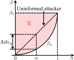
Figure 3: Illustration of the NP region $\mathcal{R}$ (shaded region), of the trade-off function $\beta_{\alpha}$, and of the MIA advantage with respect to an uninformed attacker.

As illustrated in Fig. 3, the Neyman-Pearson (NP) region $\mathcal{R}$ consists of all the achievable pairs $(\alpha,\beta)$ of TNR and FNR values that can be attained by test (10) when varying the threshold $\tau$. More precisely, including in region $\mathcal{R}$ all pairs $(\alpha^{\prime},\beta^{\prime})$ that are worse than a pair $(\alpha,\beta)$ obtained as per (11) for some threshold $\tau$, we have

$$\mathcal{R}=\left\{\left(\alpha^{\prime},\beta^{\prime}\right)\in[0,1]^{2}:\exists\tau\geq 0~{}\mathrm{s.t.}~{}\alpha^{\prime}\leq\alpha~{}\mathrm{and}~{}\beta^{\prime}\geq\beta~{}\mathrm{for}~{}(\alpha,\beta)~{}\mathrm{in}~{}\eqref{def_alpha_beta}\right\}.$$ (12)

Note, in fact, that any pair $(\alpha^{\prime},\beta^{\prime})$ with TNR $\alpha^{\prime}\leq\alpha$ and FNR $\beta^{\prime}\geq\beta$ is less desirable to the attacker than the pair $(\alpha,\beta)$.

The minimum FNR $\beta$ given a target TNR $\alpha$ is given by the trade-off function

$$\beta_{\alpha}=\inf_{(\alpha,\beta)\in\mathcal{R}}\beta.$$ (13)

For any fixed target TNR $\alpha$, a smaller trade-off function $\beta_{\alpha}$ indicates a more effective MIA. An uninformed attacker that chooses hypothesis $\mathcal{H}^{\mathrm{out}}$ with probability $\alpha$, irrespective of the output $O$, achieves the trivial trade-off $\beta_{\alpha}=\alpha$. Consequently, an effective attack must satisfy the inequality $\beta_{\alpha}<\alpha$ for at least some values of the TNR $\alpha$.

Accordingly, to characterize how well an adversary can distinguish between the two hypotheses $\mathcal{H}^{\mathrm{out}}$ and $\mathcal{H}^{\mathrm{in}}$ in (6), we introduce the MIA advantage as the difference

$$\mathrm{Adv}_{\alpha}=\alpha-\beta_{\alpha}.$$ (14)

A larger advantage $\mathrm{Adv}_{\alpha}$ indicates a more successful MIA at TNR level $\alpha$, with $\mathrm{Adv}_{\alpha}=0$ corresponding to the performance of an uninformed attacker, which produces random guesses.

III Preliminaries and Definitions

In this section, we introduce relevant background information, as well as key definitions for the analysis in the next section.

III-A Preliminaries

By (10) and (11), for a fixed TNR $\alpha$, the threshold $\tau_{\alpha}\in\mathbb{R}$ is uniquely determined by the equation [23]

$$\alpha=\mathbb{E}_{f^{\mathrm{out}}}\Big{[}\mathds{1}\Big{(}\log\Big{(}\frac{f^{\mathrm{out}}\left(O\right)}{f^{\mathrm{in}}\left(O\right)}\Big{)}\geq\tau_{\alpha}\Big{)}\Big{]},$$ (15)

and the trade-off function $\beta_{\alpha}$ can be accordingly calculated as

$$\beta_{\alpha}=\mathbb{E}_{f^{\mathrm{in}}}\Big{[}\mathds{1}\Big{(}\log\Big{(}\frac{f^{\mathrm{out}}\left(O\right)}{f^{\mathrm{in}}\left(O\right)}\Big{)}\geq\tau_{\alpha}\Big{)}\Big{]}.$$ (16)

The characterization (15)–(16) of the trade-off function $\beta_{\alpha}$ generally requires the numerical evaluation of the threshold $\tau_{\alpha}$, making it difficult to obtain analytical insights. A more convenient partial characterization is provided by the following information-theoretic outer bound.

Lemma 1 (Theorem 14.7 [23]).

Each pair $(\alpha,\beta)\in\mathcal{R}$ in the NP region (12) satisfies the inequalities

$$d(\alpha\|\beta)\leq D\left(f^{\mathrm{\rm{out}}}\|f^{\mathrm{\rm{in}}}\right),$$ (17a)

$$\mathrm{and}~{} d(\beta\|\alpha)\leq D\left(f^{\mathrm{\rm{in}}}\|f^{\mathrm{\rm{out}}}\right),$$ (17b)

where

$$D(p\|q)=\mathbb{E}_{p(x)}\Big{[}\log\frac{p(x)}{q(x)}\Big{]}$$ (18)

is the Kullback-Leibler (KL) divergence between distributions $p(x)$ and $q(x)$, and

$$d(a\|b)=a\log\Big{(}\frac{a}{b}\Big{)}+(1-a)\log\Big{(}\frac{1-a}{1-b}\Big{)}$$ (19)

is the binary KL divergence.

By the inequalities (17), the function

$$\beta_{\alpha}^{\mathrm{lb}}=\inf_{(\alpha,\beta):~{}\eqref{outer_bound}~{}\mathrm{holds}}\beta$$ (20)

is a lower bound on the optimal trade-off function (13), i.e., we have the inequality

$$\beta_{\alpha}\geq\beta_{\alpha}^{\mathrm{lb}}$$ (21)

for all $\alpha\in[0,1]$.

The following result follows from Pinsker’s inequality [24], which yields the inequalities $d(\alpha\|\beta)\geq(\alpha-\beta)^{2}/2$ and $d(\beta\|\alpha)\geq(\beta-\alpha)^{2}/2$.

Lemma 2.

The advantage (14) satisfies the upper bound

$$\mathrm{Adv}_{\alpha}\leq\alpha-\beta_{\alpha}^{\mathrm{lb}}\leq\sqrt{D\left(f^{\mathrm{\rm{out}}}\|f^{\mathrm{\rm{in}}}\right)+D\left(f^{\mathrm{\rm{in}}}\|f^{\mathrm{\rm{out}}}\right)},$$ (22)

where $\beta_{\alpha}^{\mathrm{\rm{lb}}}$ is defined in (20).

III-B Aleatoric Uncertainty

Let us write as $p^{*}_{0}=p^{*}(y=0|x_{0})$ the ground-truth probability of the true label $y_{0}$. Accordingly, the complementary probability

$$\epsilon_{a}=1-p^{*}_{0}\in\Big{[}0,1-\frac{1}{K}\Big{]}$$ (23)

can be considered to be a measure of the irreducible uncertainty about the true label $y_{0}$ for the given input $x_{0}$. This is also known as aleatoric uncertainty, or data uncertainty [6]. The aleatoric uncertainty $\epsilon_{a}$ in (23) is minimal, i.e., $\epsilon_{a}=0$, when the true label $y_{0}$ is certain, i.e., when we have $p_{0}^{*}=1$; and it is maximal, i.e., $\epsilon_{a}=1-1/K$, when the true label $y_{0}$ can be as likely as any other label, i.e., $p_{0}^{*}=1/K$ under the true distribution $p^{*}(x,y)$.

The aleatoric uncertainty imposes an irreducible upper bound on the accuracy of any classification model. When the aleatoric uncertainty is large, the selected input $x_{0}$ is inherently hard to classify, even when knowing the true distribution $p^{*}(x,y)$. Conversely, when the aleatoric uncertainty is small, the example is inherently easy to classify, at least when a sufficiently large training data set is available.

III-C Calibration

While the true probability of the class $y_{0}$ is $p_{0}^{*}$, the model assigns to it a probability $p_{0}$. A well-calibrated model is expected to output a confidence probability $p_{0}$ that is close to the ground-truth probability $p_{0}^{*}$ [25, 19]. However, machine learning models tend to be overconfident, assigning a probability $p_{0}$ larger than $p_{0}^{*}$, especially when trained with the example $(x_{0},y_{0})$ being evaluated. In fact, it is well known that the power of MIA depends on the level of overconfidence of the target model [2, 14, 1, 5, 8]. A more overconfident model tends to assign a larger probability $p_{0}$, making it easier to detect the presence of example $(x_{0},y_{0})$ in the training data set.

The calibration error is defined as the average difference between the estimated confidence probability and the ground-truth probability of the true label [25, 19]. In order to quantify the calibration performance of the target model, we define the relative calibration error as

$$\Delta=\frac{\mathbb{E}_{f^{\mathrm{in}}}\left[p_{0}\right]-p_{0}^{*}}{p_{0}^{*}},$$ (24)

which measures the relative difference between the expected confidence $\mathbb{E}_{f^{\mathrm{in}}}\left[p_{0}\right]$ generated by models trained over data sets that include the data point $(x_{0},y_{0})$ and the ground-truth probability $p^{*}_{0}\in[1/K,1]$. As mentioned, an MIA is expected to be more likely to succeed when the model is overconfident, i.e., when the relative calibration error $\Delta$ is large.

IV Analysis of the Attacker’s Advantage

In this section, we analyze the performance of LiRA in terms of the attacker’s advantage (14) for the three types of outputs defined in Sec. II-A (see also Fig. 1). We start by modeling the distributions $f^{\mathrm{out}}(O)$ and $f^{\mathrm{in}}(O)$ for the baseline case of CV observations in which the output $O$ equals the entire probability vector $p$ in (2).

IV-A Modeling the Output Distributions

As explained in the previous section, the performance of LiRA hinges on the difference between the distributions $f^{\mathrm{out}}(O)$ and $f^{\mathrm{in}}(O)$ of the observations $O$ at the attacker, with $f^{\mathrm{out}}(O)$ denoting the observation distribution when the example $(x_{0},y_{0})$ is excluded from the model’s training data set, while $f^{\mathrm{in}}(O)$ refers to the distribution when the target model is trained using the example $(x_{0},y_{0})$. Recall that randomness arises in LiRA due to the unknown data sets $\mathcal{D}^{\mathrm{out}}$ and $\mathcal{D}^{\mathrm{in}}$, which must be considered as random quantities as per (6).

All output types (3)–(5) are functions of the confidence vector $p$. Therefore, the analysis of LiRA hinges on modeling the distributions $f^{\mathrm{out}}(p)$ and $f^{\mathrm{in}}(p)$. The Dirichlet distribution provides a flexible probability density function for probability distributions over $K$ possible outputs [26]. Accordingly, while other choices are possible, we assume for our analysis that the distributions $f^{\mathrm{out}}(p)$ and $f^{\mathrm{in}}(p)$ are Dirichlet probability density functions with different parameter vectors $\gamma^{\mathrm{out}}=[\gamma_{0}^{\mathrm{out}},\ldots,\gamma_{K-1}^{\mathrm{out}}]^{\mathrm{T}}$ and $\gamma^{\mathrm{in}}=[\gamma_{0}^{\mathrm{in}},\ldots,\gamma_{K-1}^{\mathrm{in}}]^{\mathrm{T}}$, respectively. Sec. V will provide a numerical example to illustrate this assumption. Therefore, the probability density functions of the confidence vectors output by the models trained on $\mathcal{D}^{\mathrm{out}}$ or $\mathcal{D}^{\mathrm{in}}$ are given by

$$f^{z}(p)=\frac{1}{B(\gamma^{z})}\prod_{k=0}^{K-1}p_{k}^{\gamma^{z}_{k}-1},~{}~{}\mathrm{for}~{}z\in\left\{\mathrm{out},\mathrm{in}\right\},$$ (25)

where $B(\gamma^{z})=\prod_{i=0}^{K-1}\Gamma(\gamma^{z}_{i})\big{/}\Gamma(\sum_{i=0}^{K-1}\gamma^{z}_{i})$ is the multivariate Beta function expressed in terms of the Gamma function $\Gamma(x)=\int_{0}^{+\infty}t^{x-1}e^{-t}dt$.

Parameters $\gamma_{0}^{\mathrm{out}}$ and $\gamma_{0}^{\mathrm{in}}$ control the average confidence assigned to the true label by the models trained without and with $(x_{0},y_{0})$, while the remaining parameters $\gamma^{\mathrm{out}}_{1},\ldots,\gamma^{\mathrm{out}}_{K-1}$ and $\gamma^{\mathrm{in}}_{1},\ldots,\gamma^{\mathrm{in}}_{K-1}$ reflect the average confidence levels assigned by the two models to the remaining $K-1$ candidate labels. More precisely, the average confidence levels are given by [26]

$$\mathbb{E}_{f^{z}}\left[p_{k}\right]=\frac{\gamma^{z}_{k}}{\sum_{i=0}^{K-1}\gamma^{z}_{i}}~{}\mathrm{for}~{}k=0,1,\ldots,K-1,$$ (26)

where $z\in\left\{\mathrm{out},\mathrm{in}\right\}$. Considering that the confidence probability of the true label constitutes the primary source of information for the attacker, we set $\gamma^{\mathrm{out}}_{1}=\cdots=\gamma^{\mathrm{out}}_{K-1}$ and $\gamma^{\mathrm{in}}_{1}=\cdots=\gamma^{\mathrm{in}}_{K-1}$ for all other candidate classes. This assumption will facilitate the interpretation of the results of the analysis, although it is not necessary for our derivations.

Being random due to the ignorance of the attacker about the training data set, the confidence levels $p_{k}$ have variability that can be measured by the variance of the Dirichlet distribution

$$\mathrm{Var}_{f^{z}}[p_{k}]=\frac{\gamma_{k}^{z}\big{(}\sum_{i=0}^{K-1}\gamma^{z}_{i}-\gamma_{k}^{z}\big{)}}{\big{(}\sum_{i=0}^{K-1}\gamma^{z}_{i}\big{)}^{2}\big{(}\sum_{i=0}^{K-1}\gamma^{z}_{i}+1\big{)}}~{}\mathrm{for}~{}k=0,1,\ldots,K-1,$$ (27)

with $z\in\left\{\mathrm{out},\mathrm{in}\right\}$. The variance (27) accounts for the dependence of the trained model as a function of the training sets drawn from the ground-truth distribution $p^{*}(x,y)$. This model-level uncertainty, known as epistemic uncertainty [6], decreases as the size $N^{\mathrm{tr}}$ of the training data set increases. In fact, in the regime $N^{\mathrm{tr}}\rightarrow\infty$, the training data sets are fully representative of the distribution $p^{*}(x,y)$, and the probabilities $p_{k}$ tend to the ground-truth values $p^{*}_{k}$.

The possibility to decrease the epistemic uncertainty is in stark contrast to the aleatoric uncertainty introduced in the previous section, which is due to the inherent randomness of the data, and thus it does not decrease as the training set size increases. It is therefore possible to simultaneously have a high epistemic uncertainty due to limited data and a low aleatoric uncertainty for “easy” examples; and, vice versa, a high aleatoric uncertainty for “hard” examples and a low epistemic uncertainty due to access to a large training set.

To account for epistemic uncertainty, we adopt the reciprocal of the sum of Dirichlet distribution parameters, which is proportional to variance (27), i.e.,

$$\epsilon_{e}=\frac{1}{\sum_{i=0}^{K-1}\gamma_{i}^{\mathrm{out}}}=\frac{1}{\sum_{i=0}^{K-1}\gamma_{i}^{\mathrm{in}}}.$$ (28)

Furthermore, by (28), since the data set size $N^{\mathrm{tr}}$ is the same for both data sets $\mathcal{D}^{\mathrm{out}}$ and $\mathcal{D}^{\mathrm{in}}$, we assume the sum in (28) to be the same for both distributions $f^{\mathrm{out}}(p)$ and $f^{\mathrm{in}}(p)$.

Finally, using (23)–(28), we can write the Dirichlet parameters as a function of the aleatoric uncertainty $\epsilon_{a}$ in (23) and epistemic uncertainty $\epsilon_{e}$ in (28) as

$$\gamma^{\mathrm{out}}_{0}=\frac{1-\epsilon_{a}}{\epsilon_{e}},$$ (29a)

$$\mathrm{and}~{} \gamma^{\mathrm{out}}_{k}=\frac{\epsilon_{a}}{(K-1)\epsilon_{e}}~{}\mathrm{for}~{}k=1,2,\ldots,K-1,$$ (29b)

for distribution $f^{\mathrm{out}}(p)$; while, for distribution $f^{\mathrm{in}}(p)$, accounting also for the relative calibration error (24), we have

$$\gamma^{\mathrm{in}}_{0}=\frac{(1+\Delta)(1-\epsilon_{a})}{\epsilon_{e}},$$ (30a)

$$\mathrm{and}~{} \gamma^{\mathrm{in}}_{k}=\frac{\epsilon_{a}\Delta+\epsilon_{a}-\Delta}{(K-1)\epsilon_{e}}~{}\mathrm{for}~{}k=1,2,\ldots,K-1.$$ (30b)

Note that, in order to ensure the inequalities $\gamma^{z}_{k}>0$ with $z\in\left\{\mathrm{out},\mathrm{in}\right\}$ and $k=0,1,\ldots,K-1$, we have the inequality $\Delta/(1+\Delta)<\epsilon_{a}<1$. Equations (29)–(30) indicate that the average confidence generated by the model in the true label $y_{0}$ decreases with the aleatoric uncertainty $\epsilon_{a}$ and with epistemic uncertainty $\epsilon_{e}$, while also increasing with the relative calibration error $\Delta$ for the model trained with $(x_{0},y_{0})$.

IV-B Confidence Vector Disclosure

In this subsection, we leverage Lemma 2 to obtain an upper bound on the advantage of the attacker in the worst case for the target model in which the attacker observes the entire CV, i.e., $O(p)=p$. We have the following result.

Proposition 1.

The advantage of the attacker with CV disclosure (3) can be upper bounded as

$$\mathrm{Adv}^{\mathrm{\rm{CV}}}_{\alpha}\leq\Big{(}\frac{\Delta(1-\epsilon_{a})}{\epsilon_{e}}\Big{(}\psi\Big{(}\frac{(1+\Delta)(1-\epsilon_{a})}{\epsilon_{e}}\Big{)}-\psi\Big{(}\frac{1-\epsilon_{a}}{\epsilon_{e}}\Big{)}$$

$$+\psi\Big{(}\frac{\epsilon_{a}}{(K-1)\epsilon_{e}}\Big{)}-\psi\Big{(}\frac{\epsilon_{a}(1+\Delta)-\Delta}{(K-1)\epsilon_{e}}\Big{)}\Big{)}\Big{)}^{\frac{1}{2}} \triangleq\mathrm{Adv}_{\alpha}^{\mathrm{CV-ub}},$$ (31)

where $\psi(x)=\Gamma^{\prime}(x)/\Gamma(x)$ denotes the digamma function. Furthermore, using the approximation $\psi(x)\approx\ln x-1/2x$, which holds when $x\rightarrow\infty$, we obtain the approximate upper bound

$$\mathrm{Adv}_{\alpha}^{\mathrm{\rm{CV-ub}}}\approx \Big{(}\frac{\Delta(1-\epsilon_{a})}{\epsilon_{e}}\ln\Big{(}\frac{(1+\Delta)\epsilon_{a}}{(1+\Delta)\epsilon_{a}-\Delta}\Big{)}$$

$$+\frac{\Delta^{2}(1-\epsilon_{a})^{2}(K-1)}{2\epsilon_{a}((1+\Delta)\epsilon_{a}-\Delta)}+\frac{\Delta^{2}}{2(1+\Delta)}\Big{)}^{\frac{1}{2}}\triangleq\mathrm{A\widetilde{d}v}_{\alpha}^{\mathrm{\rm{CV-ub}}}.$$ (32)

Proof: The proof of (1) is detailed in Appendix -A.

The approximate bound in (1) can be used to draw some analytical insights into the attacker’s advantage, which will be validated in Sec. V by experiments. First, the bound (1) increases as the relative calibration error $\Delta$ grows, which is in line with empirical evidence that overconfident models are more vulnerable to MIA [2, 1, 14, 5].

Second, the bound (1) decreases as the aleatoric uncertainty $\epsilon_{a}$ and/or the epistemic uncertainty $\epsilon_{e}$ increase. Both a larger aleatoric uncertainty and a larger epistemic uncertainty tend to yield less confident, higher-entropy predictions, which in turn mitigates model overconfidence [6]. This ensures that the model reveals less information about the training data, potentially reducing the attack’s effectiveness. This conclusion aligns with the experimental findings in [27], where the epistemic uncertainty was increased through unlearning in order to reduce the model’s information about the target data, thereby potentially reducing the effectiveness of MIA.

IV-C True Label Confidence Disclosure

Consider now the case in which the attacker has only access to the confidence probability corresponding to the true label $y_{0}$ given input $x_{0}$, i.e., $O(p)=p_{0}$, as in [2]. The marginal probability density function for variable $p_{0}$ from the joint Dirichlet distribution (25) follows the Beta distribution. Accordingly, the probability density functions of the TLC observations output by models trained on data sets that exclude and include, respectively, the target point $(x_{0},y_{0})$, are given by

$$f^{z}(p_{0};\gamma^{z}_{0},\overline{\gamma}^{z}_{0})=\frac{1}{B(\gamma^{z}_{0},\overline{\gamma}^{z}_{0})}p_{0}^{\gamma^{z}_{0}}(1-p_{0})^{\overline{\gamma}^{z}_{0}-1},~{}\mathrm{for}~{}z\in\left\{\mathrm{out},\mathrm{in}\right\},$$ (33)

with $\overline{\gamma}^{z}_{0}=\sum_{k=1}^{K-1}\gamma^{z}_{k}$, Beta function $B(\gamma^{z}_{0},\overline{\gamma}^{z}_{0})=\Gamma(\gamma^{z}_{0})\Gamma(\overline{\gamma}^{z}_{0})\big{/}\Gamma(\gamma^{z}_{0}+\overline{\gamma}^{z}_{0})$, and Gamma function $\Gamma(x)=\int_{0}^{+\infty}t^{x-1}e^{-t}dt$. This observation yields the following result.

Proposition 2.

The advantage of the attacker with TLC disclosure (4) can be upper bounded as

$$\mathrm{Adv}^{\mathrm{\rm{TLC}}}_{\alpha}\leq\Big{(}\frac{\Delta(1-\epsilon_{a})}{\epsilon_{e}}\Big{(}\psi\Big{(}\frac{(1+\Delta)(1-\epsilon_{a})}{\epsilon_{e}}\Big{)}-\psi\Big{(}\frac{1-\epsilon_{a}}{\epsilon_{e}}\Big{)}$$

$$+\psi\Big{(}\frac{\epsilon_{a}}{\epsilon_{e}}\Big{)}-\psi\Big{(}\frac{\epsilon_{a}(1+\Delta)-\Delta}{\epsilon_{e}}\Big{)}\Big{)}\Big{)}^{\frac{1}{2}} \triangleq\mathrm{Adv}^{\mathrm{TLC-ub}}_{\alpha},$$ (34)

where $\psi(x)=\Gamma^{\prime}(x)/\Gamma(x)$ denotes the digamma function. Furthermore, using the approximation $\psi(x)\approx\ln x-1/2x$, which holds when $x\rightarrow\infty$, we obtain the approximate upper bound

$$\mathrm{Adv}^{\mathrm{TLC-ub}}_{\alpha}\approx \Big{(}\frac{\Delta(1-\epsilon_{a})}{\epsilon_{e}}\ln\Big{(}\frac{(1+\Delta)\epsilon_{a}}{(1+\Delta)\epsilon_{a}-\Delta}\Big{)}$$

$$+\frac{\Delta^{2}(1-\epsilon_{a})^{2}}{2\epsilon_{a}((1+\Delta)\epsilon_{a}-\Delta)}+\frac{\Delta^{2}}{2(1+\Delta)}\Big{)}^{\frac{1}{2}}\triangleq\mathrm{A\widetilde{d}v}^{\mathrm{TLC-ub}}_{\alpha}.$$ (35)

Proof: The upper bound $\mathrm{Adv}_{\alpha}^{\mathrm{TLC-ub}}$ in (2) and the approximate upper bound $\mathrm{A\widetilde{d}v}_{\alpha}^{\mathrm{TLC-ub}}$ in (2) can be obtained by substituting $K=2$ into (1) and (1) in Proposition 1, respectively.

By the bound (2), the MIA advantage with TLC disclosure exhibits the same general trends with respect to calibration error $\Delta$ and uncertainties $\epsilon_{a}$ and $\epsilon_{e}$ as for CV disclosure. Furthermore, comparing (2) with (1), the MIA advantage under CV observations is larger than that under TLC observations according to the derived bounds, with the gap between the two bounds growing as the number of classes, $K$, increases.

IV-D Decision Set Disclosure

In this subsection, we study the DS disclosure scenarios. To this end, we analyze a generalization of (5) that allows for randomization. Randomization is a well-established mechanism to ensure privacy [28, 22, 29], and thus it is interesting to investigate its potential role in MIA.

To this end, we consider the observation

$$O(p)=\begin{bmatrix}b_{0}\\ \vdots\\ b_{K-1}\end{bmatrix}=\mathds{1}_{T}(p\geq q)$$ (36)

where $\mathds{1}_{T}(p\geq q)$ represents a stochastic element-wise threshold function with temperature parameter $T>0$. This function returns random variables $b_{k}\in\{0,1\}$ with

$$b_{k}=\begin{cases}1&\text{with probability $\sigma_{T}(p_{k}-q)$},\\ 0&\text{with probability $\sigma_{T}(q-p_{k})$},\end{cases}$$ (37)

where $\sigma_{T}(x)=1/(1+e^{-x/T})$ represents the sigmoid function with a temperature parameter $T>0$ [30] and $b_{k}=1$ indicates the inclusion of the $k$-th label in the decision set. The stochastic DS (36) reduces to (5) in the limit $T\rightarrow 0$.

Proposition 3.

The advantage of the attacker with DS disclosure (36) can be upper bounded as

$$\mathrm{Adv}^{\mathrm{\rm{DS}}}_{\alpha}\leq\delta_{T,q}\cdot\mathrm{Adv}^{\mathrm{CV-ub}}_{\alpha} \triangleq\mathrm{Adv}^{\mathrm{DS-ub}}_{\alpha},$$ (38)

where

$$\delta_{T,q}=\Big{(}\max_{p,p^{\prime}}\frac{1}{2}\sum_{b\in\{0,1\}^{K}}\Big{|}\prod_{k=0}^{K-1}\sigma_{T}\big{(}(2b_{k}-1)(p_{k}-q)\big{)}-\prod_{k=0}^{K-1}\sigma_{T}\big{(}(2b_{k}-1)(p^{\prime}_{k}-q)\big{)}\Big{|}\Big{)}^{\frac{1}{2}},$$ (39)

with maximization over $k\times 1$ probability vectors $p$ and $p^{\prime}$, and $\mathrm{Adv}^{\mathrm{CV-ub}}_{\alpha}$ is defined in (1). Using (1) in Proposition 1, we can then obtain the approximate upper bound

$$\mathrm{A\widetilde{d}v}^{\mathrm{DS-ub}}_{\alpha}\approx\delta_{T,q}\cdot\mathrm{A\widetilde{d}v}^{\mathrm{CV-ub}}_{\alpha},$$ (40)

where $\mathrm{A\widetilde{d}v}^{\mathrm{CV-ub}}_{\alpha}$ is defined in (1).

Proof: The proof of (38) is detailed in Appendix -B.

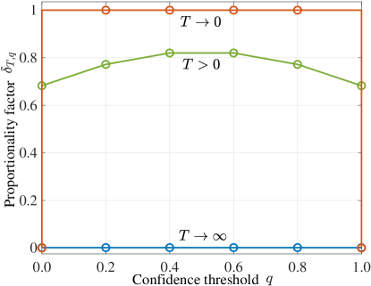
Figure 4: The proportionality factor $\delta_{T,q}$ between the advantage of DS disclosure (36) and CV disclosure (3) as a function of the confidence threshold $q$ for different values of the temperature parameter $T$ with $K=2$.

While the upper bound (40) requires numerical optimization to evaluate (39), some useful insights can be obtained from (40). In particular, the bound indicates that the attacker’s advantage under DS disclosure is proportional to that under the worst-case (for the target model) CV disclosure with a proportionality constant $\delta_{T,q}$. This constant can be proved to satisfy the inequality

$$\delta_{T,q}\leq 1,$$ (41)

reflecting the weaker power of the adversary under DS disclosure.

The proportionality factor $\delta_{T,q}$ depends on the temperature parameter $T$ as illustrated in Fig. 4 for the case $K=2$. In particular, for $T\rightarrow 0$, which corresponds to the deterministic function in (5), the constant attains the maximum value of $1$, except for the trivial cases $q=0$ and $q=1$, which yield $\delta_{T,q}=0$ as $T\rightarrow 0$. Thus, for a deterministic disclosure function, the upper bound (40) is not sufficiently tight to quantify any decrease in the attacker’s advantage. However, for any $T>0$, and thus even with minimal randomness, the bound predicts that the attacker’s advantage at first increases as $q$ grows, since a larger threshold in (36) allows to capture more information about the confidence vector $q$. However, an excessively large $q$ ends up decreasing the performance of the attacker as the predicted set $O(p)$ in (36) gets increasingly smaller. Furthermore, as $T\rightarrow\infty$, the sigmoid function equals $\sigma_{T}(x)=1/2$ and the proportionality factor equals zero, $\delta_{T,q}=0$. In this case, the attacker does not obtain any useful information, resulting in a vanishing advantage.

V Numerical Results

In this section, we provide numerical results to validate the analysis. We begin by illustrating the assumption of modeling the confidence probability vector using a Dirichlet distribution. Subsequently, we compare the analytical bounds to the actual performance of attacks based on the observations (3)–(5) as a function of calibration and uncertainty metrics. Furthermore, for attacks leveraging DS observation, we further evaluate the trade-off between prediction set size, which determines the informativeness of the predictor [31] and the attacker’s advantage. Throughout, we consider the target model to be a classifier with $K=10$ classes.

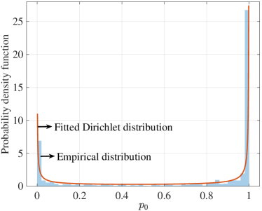
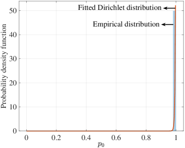
Figure 5: Empirical distributions of the confidence level $p_{0}$ and corresponding marginal of the fitted Dirichlet distributions for models trained without (left) and with (right) the target sample $(x_{0},y_{0})$.

V-A On the Dirichlet Assumption

First, to validate the use of a Dirichlet distribution to model the confidence probability, we evaluate the true distribution of the confidence vector produced by a neural network-based classifier. Following the setting in [1], we use the CIFAR-10 data set, a standard benchmark for image classification involving images classified by $K=10$ labels. To construct the training sets $\mathcal{D}^{\mathrm{out}}$ and $\mathcal{D}^{\mathrm{in}}$, we draw $N^{\mathrm{tr}}=4000$ samples at random from the overall data set. The target classification model adopts a standard convolutional neural network (CNN) with two convolution and max pooling layers, followed by a $128$-unit fully connected layer and a SoftMax output layer. The Tanh is used as the activation function, and the cross-entropy serves as the loss function. We adopt the stochastic gradient descent (SGD) optimizer with a learning rate of $0.001$, momentum of $0.9$, and weight decay of $1\times 10^{-7}$, over $100$ epochs for model training.

We collect probability vectors generated by the trained model for images corresponding to the training and test images with the truth label $0$. We then apply maximum likelihood estimation with the L-BFGS-B algorithm, a gradient descent variant tailored for large-scale optimizations [32], to fit the generated data points to Dirichlet distributions for both models trained on $\mathcal{D}^{\mathrm{out}}$ and $\mathcal{D}^{\mathrm{in}}$.

Fig. 5 illustrates the probability density functions of the confidence level $p_{0}$ for the target sample $(x_{0},y_{0})$, along with the corresponding empirical distribution obtained from the fitted Dirichlet distributions for the models trained on $\mathcal{D}^{\mathrm{out}}$ (left) and $\mathcal{D}^{\mathrm{in}}$ (right). The model is observed to be overconfident when trained by including the sample $(x_{0},y_{0})$. The empirical distributions closely align with the fitted Dirichlet distributions, confirming the flexibility of the working assumption of Dirichlet distributions for the confidence vectors. Throughout the rest of this section, we adopt this assumption.

V-B On the Impact of Calibration and Uncertainty

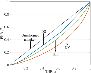
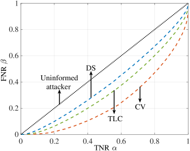
Figure 6: True trade-off function $\beta_{\alpha}$ in (16) (left) and the lower bound $\beta^{\mathrm{lb}}_{\alpha}$ in (20) (right) for CV, TLC, and DS observations with relative calibration error $\Delta=0.2$, aleatoric uncertainty $\epsilon_{a}=0.5$, epistemic uncertainty $\epsilon_{e}=0.25$, and threshold $q=0.2$.

In this subsection, to validate the analysis in Sec. IV, we compare the true trade-off function $\beta_{\alpha}$ in (16) along with the lower bound $\beta_{\alpha}^{\mathrm{lb}}$ in (20) obtained by Lemma 1 by setting the relative calibration error as $\Delta=0.2$, the aleatoric uncertainty as $\epsilon_{a}=0.5$, the and the epistemic uncertainty as $\epsilon_{e}=0.25$ in the Dirichlet parameters (29)–(30). Fig. 6 plots the true trade-off function (left) and lower bound (right) for all disclosure schemes. In particular, for DS, we consider the situation most vulnerable to MIA by applying a deterministic thresholding scheme, i.e., $T\rightarrow 0$ in (37).

The figures confirm that the derived lower bound provides a useful prediction of the relative performance of the three schemes. Specifically, both the true attacker’s advantage and the lower bound indicate that CV disclosure provides the most information to the attacker, followed by TLC and DS.

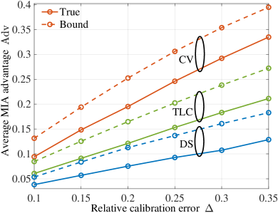
Figure 7: True advantage (14) and bounds (22) for the attacker’s advantage with CV, TLC, and DS observations as a function of relative calibration error $\Delta$ with aleatoric uncertainty $\epsilon_{a}=0.5$, epistemic uncertainty $\epsilon_{e}=0.25$, and threshold $q=0.2$.

We now turn to studying the impact of calibration and uncertainty on the attacker’s advantage. To this end, in Fig. 7, we first display the attacker’s advantage averaged over a uniformly selected TNR $\alpha$ as $\mathrm{Adv}=\mathbb{E}_{\alpha\sim U(0,1)}[\alpha-\beta_{\alpha}]$, as a function of the relative calibration error $\Delta$ with $\epsilon_{a}=0.5$ and $\epsilon_{e}=0.25$. Bound (22) in Lemma 2 and true values are again observed to be well aligned. Furthermore, confirming the empirical observations in [2, 1, 14, 5], the attacker’s advantage is seen to increase with $\Delta$. In fact, overconfident models tend to output higher confidence probabilities for the true label when trained with the target sample, which can be easily distinguished from the confidence probabilities for the other labels. Irrespective of the relative calibration error, the attacker’s advantage decreases as the model discloses less information via TLC and DS.

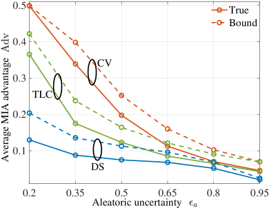
Figure 8: True advantage (14) and bounds (22) for the attacker’s advantage with CV, TLC, and DS observations as a function of aleatoric uncertainty $\epsilon_{a}$ with relative calibration error $\Delta=0.2$, epistemic uncertainty $\epsilon_{e}=0.25$, and threshold $q=0.2$.

Fig. 8 depicts the average attacker’s advantage with CV, TLC, and DS disclosures as a function of the aleatoric uncertainty $\epsilon_{a}$ with $\Delta=0.2$ and $\epsilon_{e}=0.25$. A larger aleatoric uncertainty reflects greater uncertainty in the underlying data. Accordingly, the effectiveness of attacks based on all observation types decreases and gradually approaches the theoretical lower limit of $0$. This is because the distributions of the observations produced by models trained without or with the target sample tend to become closer as the inherent data uncertainty grows. This, in turn, reduces the attacker’s ability to exploit the overconfidence in the target model for successful attacks.

Figure 9: True advantage (14) and bounds (22) for the attacker’s advantage with CV, TLC, and DS observations as a function of epistemic uncertainty $\epsilon_{e}$ with relative calibration error $\Delta=0.2$, aleatoric uncertainty $\epsilon_{a}=0.5$, and threshold $q=0.4$.

Finally, Fig. 9 shows the average attacker’s advantage as a function of the epistemic uncertainty $\epsilon_{e}$ for $\Delta=0.2$ and $\epsilon_{a}=0.5$. An increased epistemic uncertainty reflects smaller training sets, causing a larger uncertainty on the target model. Accordingly, the effectiveness of MIA decreases with $\epsilon_{e}$, becoming progressively lower due to the growing difficulty of the attacker to predict the model’s outputs when including or not the target sample $(x_{0},y_{0})$ in the training data set.

V-C Evaluating MIA with DS Disclosure

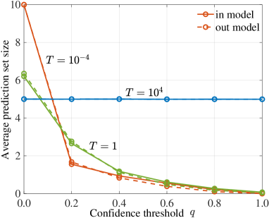
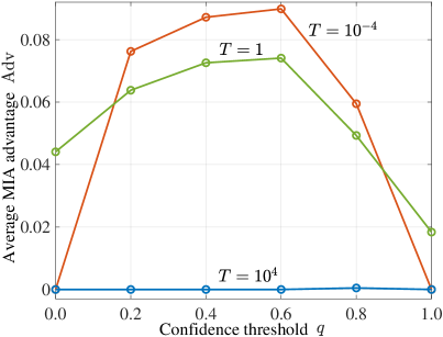
Figure 10: Average prediction set size (left) and attacker’s advantage (right) based on DS disclosure as a function of the confidence threshold $q$ with relative calibration error $\Delta=0.2$, aleatoric uncertainty $\epsilon_{a}=0.5$, epistemic uncertainty $\epsilon_{e}=0.25$.

In this final subsection, we further analyze the performance of the DS-observed attacker by studying the impact of the temperature parameter $T$ and of the confidence threshold $q$ in (36). As discussed in Sec. IV-D (see also Fig. 4), the bound (40) provides a U-shaped curve for the attacker’s advantage, as excessively small or large thresholds yield predicted sets that are nearly independent of the input $x_{0}$. In fact, as seen in Fig. 10 (left), as the threshold $q$ approaches $0$, the target model tends to produce a prediction set containing all labels, while with $q$ near $1$, it generates an empty prediction set. Neither extreme provides useful information for the attacker. The most effective attack occurs at a moderate $q$ value, here $q=0.6$, where the prediction set is expected to yield the most informative insights for the attacker. This trend is confirmed by Fig. 10 (right), which shows the average attacker’s advantage as a function of the threshold $q$ for different values of the temperature parameter $T$ in the randomized thresholding (37).

Finally, we observe that the attacker’s advantage follows the analysis in Sec. IV-D, illustrated in Fig. 4, also in terms of its dependence on the randomness of the thresholding scheme (37). As the temperature parameter $T$ approaches $0$, the thresholding scheme becomes deterministic, providing the most information to the attacker for a given threshold $q$, and resulting in the highest advantage. Conversely, as $T$ grows, the thresholding noise is so large that the attacker can obtain vanishing information about the target model, and the advantage consistently attains the theoretical lower limit of $0$.

VI Conclusions

This paper has introduced a theoretical framework to analyze the attacker’s advantage in MIAs as a function of the model’s calibration, as well as of the aleatoric and epistemic uncertainties. Following the state-of-the-art LiRA-style attacks, we regarded MIA as a hypothesis-testing problem; and we considered three typical types of observations that can be acquired by the attacker when querying the target model: confidence vector (CV), true label confidence (TLC), and decision set (DS). By making the flexible modeling assumption that the output confidence vectors follow the Dirichlet distributions, thus accounting for both aleatoric and epistemic uncertainties, we derived upper bounds on the attacker’s advantage. The bounds yield analytical insights on the impact of the relative calibration error, aleatoric uncertainty, and epistemic uncertainty on the success of MIAs. For DS disclosure, we studied for the first time the impact of the threshold and of randomization on the effectiveness of MIA.

Future work may specialize the analysis to data domains such as text, images, and tabular data, as well as to model architectures such as transformers. Additionally, from the defender’s perspective, it would be interesting to investigate the effectiveness of countermeasures to MIA such as regularization, model pruning, and data augmentation.

-A Proof of Proposition 1

The KL divergence between two Dirichlet distributions in (22) can be expressed as [33]

$$D\big{(}f^{\mathrm{out}}(p;\gamma^{\mathrm{out}})\|f^{\mathrm{in}}(p;\gamma^{\mathrm{in}})\big{)} =\ln\frac{B(\gamma^{\mathrm{in}})}{B(\gamma^{\mathrm{out}})}+\sum_{k=0}^{K-1}\big{(}\gamma^{\mathrm{out}}_{k}-\gamma^{\mathrm{in}}_{k}\big{)}\Big{(}\psi(\gamma^{\mathrm{out}}_{k})-\psi\Big{(}\sum_{i=0}^{K-1}\gamma^{\mathrm{out}}_{i}\Big{)}\Big{)},$$ (42)

where we have defined that digamma function $\psi(x)=\Gamma^{\prime}(x)/\Gamma(x)$, multivariate Beta function $B(\gamma^{\mathrm{out/in}})=\prod_{i=0}^{K-1}\Gamma(\gamma^{\mathrm{out/in}}_{i})\big{/}\Gamma(\sum_{i=0}^{K-1}\gamma^{\mathrm{out/in}}_{i})$ and Gamma function $\Gamma(x)=\int_{0}^{+\infty}t^{x-1}e^{-t}dt$. The same logic applies for $D\big{(}f^{\mathrm{in}}(p;\gamma^{\mathrm{in}})\|f^{\mathrm{out}}(p;\gamma^{\mathrm{out}})\big{)}$.

Accordingly, the square root of the symmetrized KL divergence in the approximate bound (22) in Lemma 2 given CV observations can be calculated as

$$\mathrm{Adv}^{\mathrm{CV}}_{\alpha}\leq\sqrt{D\big{(}f^{\mathrm{out}}\left(p;\gamma^{\mathrm{out}}\right)\|f^{\mathrm{in}}\left(p;\gamma^{\mathrm{in}}\right)\big{)}+D\big{(}f^{\mathrm{in}}\left(p;\gamma^{\mathrm{in}}\right)\|f^{\mathrm{out}}\left(p;\gamma^{\mathrm{out}}\right)\big{)}}\triangleq\mathrm{Adv}_{\alpha}^{\mathrm{CV-ub}},$$ (43)

by using the definitions of $\gamma_{k}^{\mathrm{out}}$ in (29) and of $\gamma_{k}^{\mathrm{in}}$ in (30).

-B Proof of Proposition 3

We leverage the strong data processing inequality [34, Proposition II.4.10][35] to obtain the upper bound of the MIA advantage given DS observations as

$$\frac{D\big{(}f^{\mathrm{out}}(b)\|f^{\mathrm{in}}(b)\big{)}}{D\big{(}f^{\mathrm{out}}(p)\|f^{\mathrm{in}}(p)\big{)}}\leq\max_{p,p^{\prime}}\left\|f(b|p)-f(b|p^{\prime})\right\|_{\mathrm{TV}}\triangleq\delta^{2}_{T,q},$$ (44)

where $\|P-Q\|_{\mathrm{TV}}$ denotes the total variance (TV) distance between distributions $P$ and $Q$. Note that we have the inequality $\delta_{T,q}^{2}\leq 1$. Accordingly, the advantage of the attacks given DS observation can be upper bounded as

$$\mathrm{Adv}^{\mathrm{DS}}_{\alpha}\leq\sqrt{D\big{(}f^{\mathrm{out}}(b)\|f^{\mathrm{in}}(b)\big{)}+D\big{(}f^{\mathrm{in}}(b)\|f^{\mathrm{out}}(b)\big{)}}=\delta_{T,q}\cdot\mathrm{Adv}^{\mathrm{CV-ub}}_{\alpha},$$ (45)

where we have used Lemma 2 and (44).

References

- [1] R. Shokri, M. Stronati, C. Song, and V. Shmatikov, “Membership inference attacks against machine learning models,” in 2017 IEEE symposium on security and privacy (SP), 2017, pp. 3–18.
- [2] N. Carlini, S. Chien, M. Nasr, S. Song, A. Terzis, and F. Tramer, “Membership inference attacks from first principles,” in 2022 IEEE Symposium on Security and Privacy (SP), 2022, pp. 1897–1914.
- [3] S. Yeom, I. Giacomelli, M. Fredrikson, and S. Jha, “Privacy risk in machine learning: Analyzing the connection to overfitting,” in 2018 IEEE 31st computer security foundations symposium (CSF), 2018, pp. 268–282.
- [4] B. Jayaraman and D. Evans, “Evaluating differentially private machine learning in practice,” in 28th USENIX Security Symposium (USENIX Security 19), 2019, pp. 1895–1912.
- [5] Z. Chen and K. Pattabiraman, “Overconfidence is a dangerous thing: Mitigating membership inference attacks by enforcing less confident prediction,” arXiv preprint arXiv:2307.01610, 2023.
- [6] E. Hüllermeier and W. Waegeman, “Aleatoric and epistemic uncertainty in machine learning: An introduction to concepts and methods,” Machine Learning, vol. 110, pp. 457–506, 2021.
- [7] J. Guo and X. Du, “Sensitivity analysis with mixture of epistemic and aleatory uncertainties,” AIAA journal, vol. 45, no. 9, pp. 2337–2349, 2007.
- [8] A. Salem, Y. Zhang, M. Humbert, P. Berrang, M. Fritz, and M. Backes, “ML-leaks: Model and data independent membership inference attacks and defenses on machine learning models,” arXiv preprint arXiv:1806.01246, 2018.
- [9] L. Song and P. Mittal, “Systematic evaluation of privacy risks of machine learning models,” in 30th USENIX Security Symposium (USENIX Security 21), 2021, pp. 2615–2632.
- [10] B. Jayaraman, L. Wang, K. Knipmeyer, Q. Gu, and D. Evans, “Revisiting membership inference under realistic assumptions,” arXiv preprint arXiv:2005.10881, 2020.
- [11] Y. Liu, Z. Zhao, M. Backes, and Y. Zhang, “Membership inference attacks by exploiting loss trajectory,” in Proceedings of the 2022 ACM SIGSAC Conference on Computer and Communications Security, 2022, pp. 2085–2098.
- [12] M. Bertran, S. Tang, M. Kearns, J. Morgenstern, A. Roth, and Z. S. Wu, “Scalable membership inference attacks via quantile regression,” arXiv preprint arXiv:2307.03694, 2023.
- [13] H. Ali, A. Qayyum, A. Al-Fuqaha, and J. Qadir, “Membership inference attacks on DNNs using adversarial perturbations,” arXiv preprint arXiv:2307.05193, 2023.
- [14] J. Ye, A. Maddi, S. K. Murakonda, V. Bindschaedler, and R. Shokri, “Enhanced membership inference attacks against machine learning models,” in Proceedings of the 2022 ACM SIGSAC Conference on Computer and Communications Security, 2022, pp. 3093–3106.
- [15] Z. Li and Y. Zhang, “Membership leakage in label-only exposures,” in Proceedings of the 2021 ACM SIGSAC Conference on Computer and Communications Security, 2021, pp. 880–895.
- [16] C. A. Choquette-Choo, F. Tramer, N. Carlini, and N. Papernot, “Label-only membership inference attacks,” in International conference on machine learning. PMLR, 2021, pp. 1964–1974.
- [17] V. Vovk, A. Gammerman, and G. Shafer, Algorithmic learning in a random world. Springer, 2005, vol. 29.
- [18] A. N. Angelopoulos and S. Bates, “A gentle introduction to conformal prediction and distribution-free uncertainty quantification,” arXiv preprint arXiv:2107.07511, 2021.
- [19] K. M. Cohen, S. Park, O. Simeone, and S. Shamai, “Calibrating AI models for wireless communications via conformal prediction,” IEEE Transactions on Machine Learning in Communications and Networking, 2023.
- [20] G. Del Grosso, G. Pichler, C. Palamidessi, and P. Piantanida, “Bounding information leakage in machine learning,” Neurocomputing, vol. 534, pp. 1–17, 2023.
- [21] E. Aubinais, E. Gassiat, and P. Piantanida, “Fundamental limits of membership inference attacks on machine learning models,” arXiv preprint arXiv:2310.13786, 2023.
- [22] C. Dwork, A. Roth et al., “The algorithmic foundations of differential privacy,” Foundations and Trends® in Theoretical Computer Science, vol. 9, no. 3–4, pp. 211–407, 2014.
- [23] Y. Polyanskiy and Y. Wu, Information Theory From Coding to Learning, 2022.
- [24] P. Jobic, M. Haddouche, and B. Guedj, “Federated learning with nonvacuous generalisation bounds,” arXiv preprint arXiv:2310.11203, 2023.
- [25] C. Guo, G. Pleiss, Y. Sun, and K. Q. Weinberger, “On calibration of modern neural networks,” in International conference on machine learning. PMLR, 2017, pp. 1321–1330.
- [26] S. Kotz, N. Balakrishnan, and N. L. Johnson, Continuous multivariate distributions, Volume 1: Models and applications. John Wiley & Sons, 2004, vol. 1.
- [27] A. Becker and T. Liebig, “Evaluating machine unlearning via epistemic uncertainty,” arXiv preprint arXiv:2208.10836, 2022.
- [28] Y. Youn, Z. Hu, J. Ziani, and J. Abernethy, “Randomized quantization is all you need for differential privacy in federated learning,” arXiv preprint arXiv:2306.11913, 2023.
- [29] D. Liu and O. Simeone, “Privacy for free: Wireless federated learning via uncoded transmission with adaptive power control,” IEEE Journal on Selected Areas in Communications, vol. 39, no. 1, pp. 170–185, 2020.
- [30] N. Papernot, A. Thakurta, S. Song, S. Chien, and Ú. Erlingsson, “Tempered sigmoid activations for deep learning with differential privacy,” in Proceedings of the AAAI Conference on Artificial Intelligence, vol. 35, no. 10, 2021, pp. 9312–9321.
- [31] M. Zecchin, S. Park, O. Simeone, and F. Hellström, “Generalization and informativeness of conformal prediction,” arXiv preprint arXiv:2401.11810, 2024.
- [32] R. H. Byrd, P. Lu, J. Nocedal, and C. Zhu, “A limited memory algorithm for bound constrained optimization,” SIAM Journal on scientific computing, vol. 16, no. 5, pp. 1190–1208, 1995.
- [33] J. Lin, “On the dirichlet distribution,” Department of Mathematics and Statistics, Queens University, pp. 10–11, 2016.
- [34] J. Cohen, J. H. Kempermann, and G. Zbaganu, Comparisons of stochastic matrices with applications in information theory, statistics, economics and population. Springer Science & Business Media, 1998.
- [35] H. He, C. Yu, and Z. Goldfeld, “Information-theoretic generalization bounds for deep neural networks,” in NeurIPS 2023 workshop: Information-Theoretic Principles in Cognitive Systems, 2023.