Reduced Order Model Enhanced Source Iteration with Synthetic Acceleration for Parametric Radiative Transfer Equation

Abstract

Applications such as uncertainty quantification, shape optimization, and optical tomography, require solving the radiative transfer equation (RTE) many times for various parameters. Efficient solvers for RTE are highly desired.

Source Iteration with Synthetic Acceleration (SISA) is one of the most popular and successful iterative solvers for RTE. Synthetic Acceleration (SA) acts as a preconditioning step to accelerate the convergence of Source Iteration (SI). After each source iteration, classical SA strategies introduce a correction to the macroscopic particle density by solving a low order approximation to a kinetic correction equation. For example, Diffusion Synthetic Acceleration (DSA) uses the diffusion limit. However, these strategies may become less effective when the underlying low order approximations are not accurate enough. Furthermore, they do not exploit low rank structures concerning the parameters of parametric problems.

To address these issues, we propose enhancing SISA with data-driven ROMs for the parametric problem and the corresponding kinetic correction equation. First, the ROM for the parametric problem can be utilized to obtain an improved initial guess. Second, the ROM for the kinetic correction equation can be utilized to design a low rank approximation to it. Unlike the diffusion limit, this ROM-based approximation builds on the kinetic description of the correction equation and leverages low rank structures concerning the parameters. We further introduce a novel SA strategy called ROMSAD. ROMSAD initially adopts our ROM-based approximation to exploit its greater efficiency in the early stage of SISA, and then automatically switches to DSA to leverage its robustness in the later stage. Additionally, we propose an approach to construct the ROM for the kinetic correction equation without directly solving it.

Through a series of numerical tests, we demonstrate the effectiveness of the proposed methods. Particularly, for a multiscale parametric pin-cell problem, ROMSAD achieves approximately $10$ times the acceleration compared to DSA.

1 Introduction

Radiative transfer equation (RTE) is a kinetic equation describing the behavior of particles (such as photons and neutrons) propagating through a background medium. It plays an important role in medical imaging [1], nuclear engineering [2], astrophysics [3], and remote sensing [4]. In applications such as shape optimization, uncertainty quantification and optical tomorgraphy, RTE needs to be solved many times for various parameters, such as boundary conditions, material properties or geometric configurations. As a result, efficient solvers for parametric RTE are highly desired.

Source Iteration with Synthetic Acceleration (SISA) is one of the most successful iterative solvers for RTE, developed over decades and widely applied in various applications. Instead of providing an exhaustive literature review for SISA, we refer readers to the review paper [5]. It is well known that, without Synthetic Acceleration (SA), Source Iteration (SI) may converge slowly for scattering dominant (optically thick) or multiscale problems [5]. SA can be seen as a preconditioning step to accelerate the convergence of SI by introducing a correction to the macroscopic particle density (also known as the scalar flux) after each source iteration. If the density correction is obtained by solving an ideal kinetic correction equation, SI will converge with at most two source iterations. However, solving this kinetic correction equation is as expensive as solving the original problem. In practice, a low order approximation to the kinetic correction equation is solved in the correction step of SA. For example, Diffusion Synthetic Acceleration (DSA) [6, 7, 8, 9] adopts its diffusion limit, Quasi-Diffusion method [10, 11, 12] uses the variable Eddington factor, and S$2$SA [13] employs a low order discrete ordinates ($S_{N}$) approximation. Despite the success of these classical SA strategies, they still have some limitations. Their effectiveness relies on the accuracy of the underlying empirical low order approximation to the kinetic correction equation. Moreover, low rank structures with respect to the parameters of parametric problems are not exploited.

To go beyond these limitations, we propose to enhance SISA by utilizing data-driven reduced order models (ROMs) for parametric RTE and the corresponding kinetic correction equation. Before presenting our methods, we briefly review the basic ideas of data-driven ROMs and their recent developments in the context of RTE. Data-driven ROMs typically follow an offline-online decomposition framework. In the offline stage, a low dimensional linear space is constructed by exploring low rank structures in the training data, i.e. solutions for parameters in a training set. In the online stage, reconstruction and prediction can be efficiently done through an interpolation or a projection based on the low dimensional space constructed offline. In recent years, ROMs for steady state and time dependent RTEs have been actively developed to utilize low rank structures in space-time domain [14], angular space [15, 16, 17], angular-time domain [18], parametric problems [19, 20, 21] and eigenvalue problems [22]. ROMs leveraging the variable Eddington factor are proposed in [23, 24, 25]. Besides data-driven ROMs, low rank tensor or matrix decompositions have been applied to design low rank solvers for RTE in [26, 27, 28, 29, 30, 31, 32, 33].

Now, we outline our strategies to leverage ROMs to accelerate the convergence of SISA.

1. The ROM for the parametric problem can be viewed as a surrogate solver for the parametric problem. It can efficiently provide an improved initial guess for SISA.

2. The ROM for the correction equation can be utilized to design a new SA strategy, called ROMSA. Instead of using empirical low order approximations to the kinetic correction equation like its diffuion limit, ROMSA employs an approximation based on a data-driven ROM for the kinetic correction equation. This approximation directly builds on the kinetic description of the correction equation and exploits low rank structures with respect to the parameters of the underlying parametric problem. Additionally, we propose an approach to construct the ROM for the kinetic correction equation without directly solving it.

In our numerical tests, we observe that ROMSA achieves more significant acceleration than DSA in the early stage of SISA. However, it may suffer from an efficiency reduction and becomes slower than DSA as iterations continue. The cause of this efficiency reduction is as follows. As source iterations continue, source terms in the kinetic correction equations for the later iterations may exhibit significant shape variations compared to those in the early stage of SISA. However, including information for source terms corresponding to the later iterations in our training data may lead to prohibitive memory costs. To improve the robustness of ROMSA without sacrificing its high efficiency in the early stage of SISA, we design a SA strategy called ROMSAD, which combines ROMSA and DSA. ROMSAD adopts ROMSA in the first few iterations of SISA to leverage its high efficiency in the early stage, and then automatically switches to DSA. In our numerical tests, we observe that, overall, ROMSAD is more efficient than DSA and more robust than ROMSA. Specifically, ROMSAD achieves approximately $10$ times the acceleration compared to DSA for a parametric multiscale pin-cell problem.

To contextualize our methods, we briefly review other methods utilizing data-driven ROMs or similar ideas to accelerate iterative solvers for RTE. For nonlinear RTEs, Dynamic Mode Decomposition (DMD) is exploited as a low rank update strategy for the SI in [34]. A neural network surrogate for the transport sweep in SI is developed in [35]. These methods focus on SI, while we concentrate on the correction step of SA. Random Singular Value Decomposition (RSVD) has been applied to build a low-rank boundary-to-boundary map of a Schwartz solver for RTE [36]. A fast solver, applying offline-online decomposition but not built on data-driven ROMs, is proposed in [37]. This method is under the framework of the Tailored Finite Point Method (TFPM). The offline stage of this method can be seen as building an efficient preconditioner for RTE based on a matrix factorization exploiting local structures given by TFPM.

The rest of this paper is organized as follows. In Sec. 2, we briefly review discrete ordinates angular discretization, upwind discontinuous Galerkin spatial discretization, and the SISA iterative solver for the steady state RTE. In Sec. 3, we build ROMs for parametric RTE and the corresponding correction equation, and introduce our ROM-based enhancement for SISA. In Sec. 4, the performance of the proposed methods is demonstrated through a series of numerical tests. In Sec. 5, we draw our conclusions and outline potential future directions.

2 Background

The steady state linear RTE with one energy group, isotropic scattering and isotropic inflow boundary conditions is:

$$\boldsymbol{v}\cdot\nabla_{\mathbf{x}}f(\mathbf{x},\boldsymbol{v})+\sigma_{t}(\mathbf{x})f(\mathbf{x},\boldsymbol{v})=\sigma_{s}(\mathbf{x})\rho(\mathbf{x})+G(\mathbf{x}),\quad\rho(\mathbf{x})=\frac{1}{4\pi}\int_{\boldsymbol{v}\in\mathbb{S}^{2}}fd\boldsymbol{v},\quad\mathbf{x}\in\Omega_{\mathbf{x}},$$ (1a)

$$f(\mathbf{x},\boldsymbol{v})=g(\mathbf{x}),\quad\mathbf{x}\in\partial\Omega_{\mathbf{x}},\;\boldsymbol{v}\cdot\boldsymbol{n}(\mathbf{x})<0.$$ (1b)

Here, $f(\mathbf{x},\boldsymbol{v})$ is the particle distribution (also known as the angular flux) with angular direction $\boldsymbol{v}\in\mathbb{S}^{2}$ at spatial location $\mathbf{x}\in\Omega_{\mathbf{x}}$, $\rho(\mathbf{x})=\frac{1}{4\pi}\int_{\boldsymbol{v}\in\mathbb{S}^{2}}f(\mathbf{x},\boldsymbol{v})d\boldsymbol{v}$ is the macroscopic density (also called scalar flux), $\sigma_{s}(\mathbf{x})\geq 0$ is the scattering cross section, $\sigma_{t}(\mathbf{x})\geq\sigma_{s}(\mathbf{x})\geq 0$ is the total cross section, $\sigma_{a}(\mathbf{x})=\sigma_{t}(\mathbf{x})-\sigma_{s}(\mathbf{x})$ is the absorption cross section, $G(\mathbf{x})$ is an isotropic source, and $\boldsymbol{n}(\mathbf{x})$ is the outward normal direction of $\Omega_{\mathbf{x}}$ at $\mathbf{x}\in\partial\Omega_{\mathbf{x}}$.

1D slab geometry: Under symmetry assumptions, RTE (1) can be further simplified in 1D slab geometry:

$$\xi\partial_{x}f(x,\xi)+\sigma_{t}(x)f(x,\xi)=\sigma_{s}(x)\rho(x)+G(x),\quad\rho(x)=\frac{1}{2}\int_{-1}^{1}f(x,\xi)d\xi,$$ (2)

where the particle distribution $f(x,\xi)$ depends on location $x\in\mathbb{R}$ and cosine of the angle between angular direction $\boldsymbol{v}$ and the $x$-axis, namely $\xi\in[-1,1]$.

In this section, we briefly review discrete ordinates angular discretization, upwind discontinuous Galerkin (DG) spatial discretization, and Source Iteration with Synthetic Acceleration (SISA).

2.1 Discrete ordinates ($S_{N}$) angular discretization

We apply discrete ordinates ($S_{N}$) method [2] in angular space. Let $\{(\boldsymbol{v}_{j},\omega_{j})\}_{j=1}^{N_{\boldsymbol{v}}}$ be a set of quadrature points in angular space and the corresponding quadrature weights satisfying $\sum_{j=1}^{N_{\boldsymbol{v}}}\omega_{j}=1$. RTE is solved at these quadrature points by approximating the normalized integral term, $\rho(\mathbf{x})=\frac{1}{4\pi}\int_{\boldsymbol{v}\in\mathbb{S}^{2}}f(\mathbf{x},\boldsymbol{v})d\boldsymbol{v}$, with the associated quadrature rule:

$$(\boldsymbol{v}_{j}\cdot\nabla_{x}+\sigma_{t}(\mathbf{x}))f(\mathbf{x},\boldsymbol{v}_{j})=\sigma_{s}(\mathbf{x})\rho(\mathbf{x})+G(\mathbf{x}),\quad\rho(\mathbf{x})=\sum_{j=1}^{N_{\boldsymbol{v}}}\omega_{j}f(\mathbf{x},\boldsymbol{v}_{j})$$ (3a)

$$f(\mathbf{x},\boldsymbol{v}_{j})=g(\mathbf{x}),\quad\mathbf{x}\in\partial\Omega_{\mathbf{x}},\;\boldsymbol{v}_{j}\cdot\boldsymbol{n}(\mathbf{x})<0.$$ (3b)

For 1D slab geometry, we use Gauss-Legendre quadrature points. For 2D X-Y geometry with $\mathbb{S}^{2}$ as the angular space, we use Chebyshev-Legendre (CL) points. CL quadrature is the tensor product of Chebyshev rule for the unit circle and Gauss-Legendre rule for $\boldsymbol{v}_{z}\in[-1,1]$. The quadrature points and weights of the $N_{\phi}$-points normalized Chebyshev quadrature rule for the unit circle is

$$\left\{(\phi_{j},\omega_{\phi,j}):\;\phi_{j}=\frac{j\pi}{N_{\phi}}-\frac{\pi}{2N_{\phi}}\;\text{and}\;\omega^{\phi}_{j}=\frac{1}{N_{\phi}},\;j=1,\dots,N_{\phi}\right\}.$$

Let $\{(v_{z,j},\omega_{z,j})\}_{j=1}^{N_{v_{z}}}$ denote quadrature points and weights of the $N_{v_{z}}$-points normalized Gauss-Legendre rule for $[-1,1]$. The quadrature points and weights of the CL$(N_{\phi},N_{v_{z}})$ quadrature rule, $(\boldsymbol{v}_{j},\omega_{j})$, are defined as

$$\boldsymbol{v}_{j}=\left(\cos(\phi_{j_{1}})\sqrt{1-v_{z,j_{2}}^{2}},\sin(\phi_{j_{1}})\sqrt{1-v_{z,j_{2}}^{2}},v_{z,j_{2}}\right),\;\omega_{j}=\omega_{\phi,j_{1}}\omega_{v_{z},j_{2}},$$

where $1\leq j_{1}\leq N_{\phi}$, $1\leq j_{2}\leq N_{v_{z}}$ and $j=(j_{2}-1)N_{\phi}+j_{1}$. Normalized integral on $\mathbb{S}^{2}$ can be approximated by this quadrature rule as $\frac{1}{4\pi}\int_{\boldsymbol{v}\in\mathbb{S}^{2}}f(\boldsymbol{v})d\boldsymbol{v}\approx\sum_{j=1}^{N_{\phi}N_{v_{z}}}\omega_{j}f(\boldsymbol{v}_{j}).$ Other popular choices for angular discretization of $\mathbb{S}^{2}$ include Lebedev quadratures rule [38] and $T_{N}$ quadrature rules [39].

2.2 Upwind discontinuous Galerkin spatial discretization

We apply upwind discontinuous Galerkin (DG) spatial discretization, because it is an asymptotic preserving (locking free in optically thick regions) scheme [40, 41], which is able to capture the correct diffusion limit without resolving small mean free path of particles.

Consider 2D $X$-$Y$ geometry with a rectangular computational domain $\Omega_{\mathbf{x}}=[x_{l},x_{r}]\times[y_{l},y_{r}]$. Let $\mathcal{T}_{h}=\{\mathcal{T}_{i}\}_{i=1}^{N_{\mathbf{x}}}$ be a partition of $\Omega_{\mathbf{x}}$ with $\mathcal{T}_{i}$’s being rectangles. We seek the solution in the discrete space

$$U_{h}^{K}(\mathcal{T}_{h}):=\{u(\mathbf{x}):u(\mathbf{x})|_{\mathcal{T}_{i}}\in Q^{K}(\mathcal{T}_{i}),1\leq i\leq N_{\mathbf{x}}\},$$ (4)

where $Q^{K}(\mathcal{T}_{i})$ is the bi-variate polynomial space whose degree in each direction is at most $K$ on the element $\mathcal{T}_{i}$. Denote the set of cell edges as $\partial\mathcal{T}_{h}$ and the set of edges on the inflow boundary for $\boldsymbol{v}_{j}$ as

$$\partial\mathcal{T}_{h,j}^{(\textrm{ibc})}=\{\mathcal{E}:\mathcal{E}\in\partial\mathcal{T}_{h},\;\mathcal{E}\subset\partial\Omega_{\mathbf{x}},\;\boldsymbol{v}_{j}\cdot\boldsymbol{n}(\mathbf{x})<0,\forall\mathbf{x}\in\mathcal{E}\},$$

where $\boldsymbol{n}(\mathbf{x})$ is the outward normal direction of $\Omega_{\mathbf{x}}$ at $\mathbf{x}$.

Applying upwind DG spatial discretization to (3), we seek $f_{h}(\mathbf{x},\boldsymbol{v}_{j})\in U_{h}^{K}(\mathcal{T}_{h})$, $j=1,\dots,N_{\boldsymbol{v}}$ satisfying $\forall\phi_{h}(\mathbf{x})\in U_{h}^{K}(\mathcal{T}_{h}),$

$$-\sum_{i=1}^{N_{\mathbf{x}}} \int_{\mathcal{T}_{i}}\Big{(}\boldsymbol{v}_{j}\cdot\nabla\phi_{h}(\mathbf{x})\Big{)}f_{h}(\mathbf{x},\boldsymbol{v}_{j})d\mathbf{x}+\sum_{\mathcal{E}\in\partial\mathcal{T}_{h}\setminus\partial\mathcal{T}_{h,j}^{(\textrm{ibc})}}\int_{\mathcal{E}}\widehat{{\bf{H}}}(\boldsymbol{v}_{j},f_{h},\boldsymbol{n}(\mathbf{x}))\phi_{h}(\mathbf{x})d\mathbf{x}+\sum_{i=1}^{N_{\mathbf{x}}}\int_{\mathcal{T}_{i}}\sigma_{t}(\mathbf{x})f_{h}(\mathbf{x},\boldsymbol{v}_{j})\phi_{h}(\mathbf{x})d\mathbf{x}$$

$$= \sum_{i=1}^{N_{\mathbf{x}}}\int_{\mathcal{T}_{i}}\sigma_{s}(\mathbf{x})\rho_{h}(\mathbf{x})\phi_{h}(\mathbf{x})d\mathbf{x}+\sum_{i=1}^{N_{\mathbf{x}}}\int_{\mathcal{T}_{i}}G(\mathbf{x})\phi_{h}(\mathbf{x})d\mathbf{x}-\sum_{\mathcal{E}\in\partial\mathcal{T}_{h,j}^{(\textrm{ibc})}}\int_{\mathcal{E}}g(\mathbf{x})\phi_{h}(\mathbf{x})\boldsymbol{v}_{j}\cdot\boldsymbol{n}(\mathbf{x})d\mathbf{x}.$$ (5)

Here, $\rho_{h}(\mathbf{x})=\sum_{j=1}^{N_{\boldsymbol{v}}}\omega_{j}f_{h}(\mathbf{x},\boldsymbol{v}_{j})$. The upwind numerical flux $\widehat{{\bf{H}}}(\boldsymbol{v}_{j},f_{h},\boldsymbol{n}(\mathbf{x}))$ along the edge $\mathcal{E}$ for an element $\mathcal{T}_{i}=\mathcal{T}^{-}$ with the neighboring element $\mathcal{T}^{+}$, is defined as

$$\widehat{{\bf{H}}}(\boldsymbol{v}_{j},f_{h},\boldsymbol{n}(\mathbf{x}))=\frac{\boldsymbol{v}_{j}\cdot\boldsymbol{n}(\mathbf{x})}{2}\Big{(}f_{h}^{+}(\mathbf{x},\boldsymbol{v}_{j})+f_{h}^{-}(\mathbf{x},\boldsymbol{v}_{j})\Big{)}+\frac{|\boldsymbol{v}_{j}\cdot\boldsymbol{n}(\mathbf{x})|}{2}\Big{(}f_{h}^{-}(\mathbf{x},\boldsymbol{v}_{j})-f_{h}^{+}(\mathbf{x},\boldsymbol{v}_{j})\Big{)},$$ (6)

where $f_{h}^{\pm}(\mathbf{x},\boldsymbol{v}_{j})$ is the restriction of $f_{h}(\mathbf{x},\boldsymbol{v}_{j})$ to $\mathcal{T}^{\pm}$, and $\boldsymbol{n}(\mathbf{x})$ is the unit outward normal direction at $\mathbf{x}\in\mathcal{E}$ with respect to the element $\mathcal{T}_{i}=\mathcal{T}^{-}$.

We further rewrite the DG scheme to its matrix-vector form. Let $\{\phi_{i}(\mathbf{x})\}_{i=1}^{N_{\textrm{DOF}}}$ be an orthonormal basis for $U_{h}^{K}(\mathcal{T}_{h})$. Then, $f_{h}(\mathbf{x},\boldsymbol{v}_{j})$ and $\rho_{h}(\mathbf{x})$ can be expanded as

$$f_{h}(\mathbf{x},\boldsymbol{v}_{j})=\sum_{i=1}^{N_{\textrm{DOF}}}\alpha_{i}^{f}(\boldsymbol{v}_{j})\phi_{i}(\mathbf{x})\quad\text{and}\quad\rho_{h}(\mathbf{x})=\sum_{i=1}^{N_{\textrm{DOF}}}\alpha_{i}^{\rho}\phi_{i}(\mathbf{x}),\;\text{with}\;\alpha_{i}^{\rho}=\sum_{j=1}^{N_{\boldsymbol{v}}}\omega_{j}\alpha_{i}^{f}(\boldsymbol{v}_{j}).$$ (7)

Define $\boldsymbol{f}_{j}=\left(\alpha_{1}^{f}(\boldsymbol{v}_{j}),\dots,\alpha_{N_{\textrm{DOF}}}^{f}(\boldsymbol{v}_{j})\right)^{T}\in\mathbb{R}^{N_{\textrm{DOF}}}$, $\boldsymbol{\rho}=\left(\alpha_{1}^{\rho},\dots,\alpha_{N_{\textrm{DOF}}}^{\rho}\right)^{T}\in\mathbb{R}^{N_{\textrm{DOF}}}$. Then, the DG scheme (5) can be written in its matrix-vector form:

$$({\bf{D}}_{j}+{\mathbf{\Sigma}}_{t})\boldsymbol{f}_{j}={\mathbf{\Sigma}}_{s}\boldsymbol{\rho}+\boldsymbol{G}+\boldsymbol{g}_{j}^{(\textrm{bc})}={\mathbf{\Sigma}}_{s}\boldsymbol{\rho}+\widetilde{\boldsymbol{G}}_{j},\;\boldsymbol{\rho}=\sum_{j=1}^{N_{\boldsymbol{v}}}\omega_{j}\boldsymbol{f}_{j},\quad j=1,\dots,N_{\boldsymbol{v}},$$ (8)

where ${\bf{D}}_{j},{\mathbf{\Sigma}}_{s},{\mathbf{\Sigma}}_{t}\in\mathbb{R}^{N_{\textrm{DOF}}\times N_{\textrm{DOF}}}$, $\boldsymbol{G},\boldsymbol{g}_{j}^{(\textrm{bc})}\in\mathbb{R}^{\textrm{DOF}}$ and $\widetilde{\boldsymbol{G}}_{j}=\boldsymbol{G}+\boldsymbol{g}_{j}^{(\textrm{bc})}$ are defined as:

$$({\bf{D}}_{j})_{kl}=-\sum_{i=1}^{N_{x}}\int_{\mathcal{T}_{i}}(\boldsymbol{v}_{j}\cdot\nabla\phi_{k}(\mathbf{x}))\phi_{l}(\mathbf{x})d\mathbf{x}+\sum_{\mathcal{E}\in\partial\mathcal{T}_{h}\setminus\partial\mathcal{T}_{h,j}^{(\textrm{ibc})}}\int_{\mathcal{E}}\widehat{{\bf{H}}}\left(\boldsymbol{v}_{j},\phi_{l},\boldsymbol{n}(\mathbf{x})\right)\phi_{k}(\mathbf{x})d\mathbf{x},$$ (9a)

$$({\mathbf{\Sigma}}_{t})_{kl}=\sum_{i=1}^{N_{x}}\int_{\mathcal{T}_{i}}\sigma_{t}(\mathbf{x})\phi_{k}(\mathbf{x})\phi_{l}(\mathbf{x})d\mathbf{x},\quad({\mathbf{\Sigma}}_{s})_{kl}=\sum_{i=1}^{N_{x}}\int_{\mathcal{T}_{i}}\sigma_{s}(\mathbf{x})\phi_{k}(\mathbf{x})\phi_{l}(\mathbf{x})d\mathbf{x},$$ (9b)

$$(\boldsymbol{G})_{k}=\sum_{i=1}^{N_{x}}\int_{\mathcal{T}_{i}}G(\mathbf{x})\phi_{k}(\mathbf{x})d\mathbf{x},\quad(\boldsymbol{g}_{j}^{(\textrm{bc})})_{k}=-\sum_{\mathcal{E}\in\partial\mathcal{T}_{h,j}^{(\textrm{ibc})}}\int_{\mathcal{E}}g(\mathbf{x})\phi_{k}(\mathbf{x})\boldsymbol{v}_{j}\cdot\boldsymbol{n}(\mathbf{x})d\mathbf{x}.$$ (9c)

Let $\boldsymbol{f}=(\boldsymbol{f}_{1}^{T},\dots,\boldsymbol{f}_{N_{\boldsymbol{v}}}^{T})^{T}\in\mathbb{R}^{N_{\boldsymbol{v}}N_{\textrm{DOF}}}$, then (8) can be rewritten as a coupled linear system

$$\mathbf{A}\boldsymbol{f}=\left(\begin{matrix}{\bf{D}}_{1}+{\mathbf{\Sigma}}_{t}-\omega_{1}{\mathbf{\Sigma}}_{s}&-\omega_{2}{\mathbf{\Sigma}}_{s}&\dots&-\omega_{N_{\boldsymbol{v}}}{\mathbf{\Sigma}}_{s}\\ -\omega_{1}{\mathbf{\Sigma}}_{s}&{\bf{D}}_{2}+{\mathbf{\Sigma}}_{t}-\omega_{2}{\mathbf{\Sigma}}_{s}&\dots&-\omega_{N_{\boldsymbol{v}}}{\mathbf{\Sigma}}_{s}\\ \vdots&\vdots&\vdots&\vdots\\ -\omega_{1}{\mathbf{\Sigma}}_{s}&-\omega_{2}{\mathbf{\Sigma}}_{s}&\dots&{\bf{D}}_{N_{\boldsymbol{v}}}+{\mathbf{\Sigma}}_{t}-\omega_{N_{\boldsymbol{v}}}{\mathbf{\Sigma}}_{s}\end{matrix}\right)\left(\begin{matrix}\boldsymbol{f}_{1}\\ \boldsymbol{f}_{2}\\ \vdots\\ \boldsymbol{f}_{N_{\boldsymbol{v}}}\end{matrix}\right)=\left(\begin{matrix}\widetilde{\boldsymbol{G}}_{1}\\ \widetilde{\boldsymbol{G}}_{2}\\ \vdots\\ \widetilde{\boldsymbol{G}}_{N_{\boldsymbol{v}}}\end{matrix}\right)=\mathbf{b}$$ (10)

2.3 Source Iteration with Synthetic Acceleration

We briefly review basic ideas of Source Iteration with Synthetic Acceleration (SISA) [5]. Before delving into details, we present the overall workflow of SISA in Alg. 1.

Algorithm 1 Source Iteration with Synthetic Acceleration (SISA) to solve (8)

  Given initial guess: $\boldsymbol{\rho}^{(0)}$, tolerance $\epsilon_{\textrm{SISA}}$, and the maximum number of iterations allowed $N_{\textrm{iter}}$.

  Source iteration: solve $({\bf{D}}_{j}+{\mathbf{\Sigma}}_{t})\boldsymbol{f}_{j}^{(1)}=\widetilde{\boldsymbol{G}}_{j}+{\mathbf{\Sigma}}_{s}\boldsymbol{\rho}^{(0)}$, $j=1,\dots,N_{\boldsymbol{v}}$.

  Update the density as $\boldsymbol{\rho}^{(1,*)}=\sum_{j=1}^{N_{\boldsymbol{v}}}\omega_{j}\boldsymbol{f}_{j}^{(1)}$.

  if  $||\rho^{(1,*)}-\rho^{(0)}||_{\infty}<\epsilon_{\textrm{SISA}}$, then

     return $\boldsymbol{\rho}^{(1,*)}$ and $\boldsymbol{f}^{(1)}$ as our solutions.

  end if

  Correction: solve a correction equation to obtain the correction $\delta\boldsymbol{\rho}^{(1)}$.

  Update the density as $\boldsymbol{\rho}^{(1)}=\boldsymbol{\rho}^{(1,*)}+\delta\boldsymbol{\rho}^{(1)}$.

  for $l=2:N_{\textrm{iter}}$ do

     Source iteration: solve $({\bf{D}}_{j}+{\mathbf{\Sigma}}_{t})\boldsymbol{f}_{j}^{(l)}=\widetilde{\boldsymbol{G}}_{j}+{\mathbf{\Sigma}}_{s}\boldsymbol{\rho}^{(l-1)}$, $j=1,\dots,N_{\boldsymbol{v}}$.

     Update the density as $\boldsymbol{\rho}^{(l,*)}=\sum_{j=1}^{N_{\boldsymbol{v}}}\omega_{j}\boldsymbol{f}_{j}^{(l)}$.

     if  $||\rho^{(l,*)}-\rho^{(l-1)}||_{\infty}<\epsilon_{\textrm{SISA}}$, then

        return $\boldsymbol{\rho}^{(l,*)}$ and $\boldsymbol{f}^{(l)}$ as the solution.

     end if

     Correction: solve a correction equation to obtain the correction $\delta\boldsymbol{\rho}^{(l)}$.

     Update the density as $\boldsymbol{\rho}^{(l)}=\boldsymbol{\rho}^{(l,*)}+\delta\boldsymbol{\rho}^{(l)}$.

  end for

Source Iteration (SI): In the linear system $\mathbf{A}\in\mathbb{R}^{N_{\boldsymbol{v}}N_{\textrm{DOF}}\times N_{\boldsymbol{v}}N_{\textrm{DOF}}}$ (defiend in (10)), $\boldsymbol{f}_{j}$’s are coupled through the integral term ${\mathbf{\Sigma}}_{s}\boldsymbol{\rho}=\sum_{j=1}^{N_{\boldsymbol{v}}}\omega_{j}{\mathbf{\Sigma}}_{s}\boldsymbol{f}_{j}$. To avoid directly solving the huge coupled system $\mathbf{A}$, SI decouples $\boldsymbol{f}_{j}$ in each iteration by freezing the density $\boldsymbol{\rho}$. Specifically, in the $l$-th source iteration $(l\geq 1)$, given the density determined by the previous iteration or the initial guess $\boldsymbol{\rho}^{(l-1)}$, we update the solution by solving

$$({\bf{D}}_{j}+{\mathbf{\Sigma}}_{t})\boldsymbol{f}_{j}^{(l)}={\mathbf{\Sigma}}_{s}\boldsymbol{\rho}^{(l-1)}+\boldsymbol{G}+\boldsymbol{g}_{j}^{(\textrm{bc})},\;j=1,\dots,N_{\boldsymbol{v}}.$$ (11)

Without Synthetic Acceleration (SA), the density is updated as $\boldsymbol{\rho}^{(l)}=\boldsymbol{\rho}^{(l,*)}=\sum_{j=1}^{N_{\boldsymbol{v}}}\omega_{j}\boldsymbol{f}_{j}^{(l)}$. With upwind DG spatial discretization, ${\bf{D}}_{j}+{\mathbf{\Sigma}}_{t}$ is a block lower triangular matrix, when a proper ordering of elements determined by the upwind direction for $\boldsymbol{v}_{j}$ is applied. Consequently, the decoupled linear system (11) can be efficiently solved in a matrix-free manner by a transport sweep [5].

Synthetic Acceleration (SA): It is well known that vanilla SI can suffer from arbitrarily slow convergence [5]. SA can be viewed as a preconditioning step to accelerate its convergence. SA introduces a correction to the density after each source iteration:

$$\boldsymbol{\rho}^{(l)}=\boldsymbol{\rho}^{(l,*)}+\delta\boldsymbol{\rho}^{(l)},\quad\boldsymbol{\rho}^{(l,*)}=\sum_{j=1}^{N_{\boldsymbol{v}}}\omega_{j}\boldsymbol{f}_{j}^{(l)}.$$ (12)

Let $\boldsymbol{f}_{j}$ be the exact solution to (8). The ideal density correction is

$$\delta\boldsymbol{\rho}^{(l)}=\sum_{j=1}^{N_{\boldsymbol{v}}}\omega_{j}\delta\boldsymbol{f}^{(l)},\quad\delta\boldsymbol{f}_{j}^{(l)}=\boldsymbol{f}_{j}-\boldsymbol{f}_{j}^{(l)}.$$ (13)

One can show that the ideal correction $\delta\boldsymbol{f}_{j}^{(l)}$ satisfies the following discrete kinetic correction equation:

$$({\bf{D}}_{j}+{\mathbf{\Sigma}}_{t})\delta\boldsymbol{f}_{j}^{(l)}={\mathbf{\Sigma}}_{s}\delta\boldsymbol{\rho}^{(l)}+{\mathbf{\Sigma}}_{s}\left(\boldsymbol{\rho}^{(l,*)}-\boldsymbol{\rho}^{(l-1)}\right),\;j=1,\dots,N_{\boldsymbol{v}},$$ (14a)

$$\delta\boldsymbol{\rho}^{(l)}=\sum_{j=1}^{N_{\boldsymbol{v}}}\omega_{j}\delta\boldsymbol{f}_{j}^{(l)},$$ (14b)

which can be rewritten as

$$\mathbf{A}\delta\boldsymbol{f}^{(l)}=\delta\mathbf{b}^{(l)},$$ (15)

where $\mathbf{A}$ is defined in (10), $\delta\boldsymbol{f}^{(l)}=\left((\delta\boldsymbol{f}_{1}^{(l)})^{T},\dots,(\delta\boldsymbol{f}^{(l)}_{N_{\boldsymbol{v}}})^{T}\right)^{T}$, and

$$\delta\mathbf{b}^{(l)}=\underbrace{\left(({\mathbf{\Sigma}}_{s}(\boldsymbol{\rho}^{(l,*})-\boldsymbol{\rho}^{(l-1)}))^{T},\dots,({\mathbf{\Sigma}}_{s}(\boldsymbol{\rho}^{(l,*)}-\boldsymbol{\rho}^{(l-1)}))^{T}\right)^{T}}_{\text{Repeat }N_{v}\text{\;times}}.$$

Equation (14) is the $S_{N}$-DG discretization of the kinetic correction equation

$$\boldsymbol{v}\cdot\nabla_{\mathbf{x}}\delta f^{(l)}(\mathbf{x},\boldsymbol{v})+\sigma_{t}(\mathbf{x})\delta f^{(l)}(\mathbf{x},\boldsymbol{v})=\sigma_{s}\delta\rho^{(l)}(\mathbf{x})+\sigma_{s}(\mathbf{x})(\rho^{(l,*)}(\mathbf{x})-\rho^{(l-1)}(\mathbf{x})),\quad\mathbf{x}\in\Omega_{\mathbf{x}},$$ (16a)

$$\delta\rho^{(l)}(\mathbf{x})=\frac{1}{4\pi}\int_{\mathbb{S}^{2}}\delta f^{(l)}(\mathbf{x},\boldsymbol{v})d\boldsymbol{v},\quad\mathbf{x}\in\Omega_{\mathbf{x}}$$ (16b)

$$\delta f^{(l)}(\mathbf{x},\boldsymbol{v})=0,\quad\mathbf{x}\in\partial\Omega_{\mathbf{x}},\;\boldsymbol{v}\cdot\boldsymbol{n}(\mathbf{x})<0,$$ (16c)

which is a RTE with the isotropic source $\sigma_{s}(\mathbf{x})(\rho^{(l,*)}(\mathbf{x})-\rho^{(l-1)}(\mathbf{x}))$ and zero inflow boundary conditions. If one exactly solves the kinetic correction equation (14), the SI converges with at most two iterations, because the solution of (8) satisfies

$$\boldsymbol{\rho}=\boldsymbol{\rho}^{(1)}=\boldsymbol{\rho}^{(1,*)}+\delta\boldsymbol{\rho}^{(1)}\quad\text{and}\quad\boldsymbol{f}_{j}=\boldsymbol{f}_{j}^{(2)}=({\bf{D}}_{j}+{\mathbf{\Sigma}}_{t})^{-1}({\mathbf{\Sigma}}_{s}\boldsymbol{\rho}+\boldsymbol{G}+\boldsymbol{g}_{j}^{\textrm{(bc)}}).$$

However, solving the kinetic correction equation (14) is as expensive as directly solving (8).

In practice, instead of the kinetic correction equation (14), a computationally cheap low order approximation to it is solved in the correction step. For example, Diffusion Synthetic Acceleration (DSA) [6, 7, 8, 9, 5] adopts the diffusion limit of the kinetic correction equation (16)

$$-\nabla_{\mathbf{x}}\cdot\left(\frac{1}{\sigma_{s}}{\bf{D}}_{\boldsymbol{v}}(\nabla_{\mathbf{x}}\delta\rho^{(l)})\right)=-\sigma_{a}\delta\rho^{(l)}+\sigma_{s}(\rho^{(l,*)}-\rho^{(l-1)}),$$ (17)

where ${\bf{D}}_{\boldsymbol{v}}=\textrm{diag}\left(\frac{1}{4\pi}\int_{\boldsymbol{v}\in\mathbb{S}^{2}}\boldsymbol{v}_{x}^{2}d\boldsymbol{v},\frac{1}{4\pi}\int_{\boldsymbol{v}\in\mathbb{S}^{2}}\boldsymbol{v}_{y}^{2}d\boldsymbol{v},\frac{1}{4\pi}\int_{\boldsymbol{v}\in\mathbb{S}^{2}}\boldsymbol{v}_{z}^{2}d\boldsymbol{v}\right).$ Quasi-Diffusion method [10, 11, 12] uses the variable Eddington factor, and S$2$SA [13] employs a low order discrete ordinates ($S_{N}$) approximation. The effectiveness of these methods relies on the accuracy of their underlying low order approximations. For example, SI with DSA (SI-DSA) may converge slowly, if the kinetic correction equation is far from its diffusion limit [5].

3 Reduced order model enhanced SISA

In applications such as uncertainty quantification, shape optimization and inverse problems, RTE needs to be solved many times for various parameters. Low rank structures with respect to the parameters of these parametric problems are not exploited by classical SA strategies like DSA. We propose utilizing data-driven reduced order models (ROMs) for these parametric problems and their corresponding kinetic correction equations to enhance SISA by identifying and leveraging these low rank structures.

The ROM for the parametric problem can be exploited to provide an improved initial guess for SISA. Additionally, the ROM for the kinetic correction equation can be exploited to design a low rank approximation to the kinetic correction equation (14). Unlike empirical low order approximations such as the diffusion limit, this ROM-based low rank approximation directly builds on the kinetic description of the correction equation and leverages low rank structures with respect to the parameters. Furthermore, novel SA strategies can be developed based on this approximation.

This section is organized as follows. In Sec. 3.1 we first build a ROM for parametric RTE following [21] and then use the constructed ROM to provide an initial guess for SISA. In Sec. 3.2, we propose a strategy to build a ROM for the kinetic correction equation without directly solving it, and then design two SA strategies built on this ROM for the kinetic correction equation.

3.1 ROM based initial guess

We first construct a ROM for parametric RTE following [21], and then utilize the constructed ROM to provide an improved initial guess for the SISA.

3.1.1 ROM for parametric RTE

Following [21], we employ Proper Orthogonal Decomposition (POD) [42, 43] to build a ROM for parametric RTE. POD applies an offline-online decomposition framework. In the online stage, we seek reduced order solutions in a reduced order space constructed offline. The dimension of this reduced order space is much smaller than $N_{v}N_{\textrm{DOF}}$, resulting in very efficient prediction online. In the offline stage, we construct the reduced order space by extracting low rank structures from the training data. The details of this procedure are as follows.

Offline reduced order space construction: Let $\mathcal{P}_{\textrm{train}}=\{{\boldsymbol{\mu}}_{j}\in\mathbb{R}^{p}\}_{j=1}^{N_{\textrm{train}}}$ be a training set of parameters, such as the strength of scattering and absorption cross sections, boundary conditions and source terms. Denote the solution corresponding to a parameter ${\boldsymbol{\mu}}$ as $\boldsymbol{f}^{{\boldsymbol{\mu}}}$, also called a snapshot. The snapshot matrix determined by the training set is defined as

$$\mathbf{F}=\left(\boldsymbol{f}^{{\boldsymbol{\mu}}_{1}},\boldsymbol{f}^{{\boldsymbol{\mu}}_{2}},\dots,\boldsymbol{f}^{{\boldsymbol{\mu}}_{N_{\textrm{train}}}}\right).$$ (18)

Each column of the snapshot matrix $\mathbf{F}$ is a full order solution corresponding to a parameter ${\boldsymbol{\mu}}\in\mathcal{P}_{\textrm{train}}$. These solutions can be obtained by solving (8) with SI-DSA.

To identify low rank structures in the training data, we compute the singular value decomposition (SVD) of the snapshot matrix $\mathbf{F}$:

$$\mathbf{F}=\mathbf{U}\mathbf{\Lambda}\mathbf{V}^{T},$$ (19)

where $\mathbf{U}\in\mathbb{R}^{N_{\boldsymbol{v}}N_{\textrm{DOF}}\times N_{\boldsymbol{v}}N_{\textrm{DOF}}}$, $\mathbf{V}\in\mathbb{R}^{N_{\textrm{train}}\times{N_{\textrm{train}}}}$ are orthogonal matrices, and the $k$-th diagonal element of $\mathbf{\Lambda}\in\mathbb{R}^{N_{\boldsymbol{v}}N_{\textrm{DOF}}\times N_{\textrm{train}}}$, $\lambda_{k}$, is the $k$-th largest singular value of $\mathbf{F}$. Given an error tolerance $\epsilon_{\textrm{POD}}$, we determine the dimension of the desired reduced order space $r_{p}$ as

$$r_{p}=\arg\min_{l}\frac{\sum_{k=1}^{l}{\lambda_{k}}}{\textrm{trace}(\mathbf{\Lambda})}\geq 1-\epsilon_{\textrm{POD}}.$$ (20)

The POD basis $\mathbf{U}_{r_{p}}$ is defined as the first $r_{p}$ columns of $\mathbf{U}$. The constructed reduced order space is the space determined by columns of $\mathbf{U}_{r_{p}}$. In the online stage, we seek reduced order solutions in this space.

Online prediction: In the online stage, to efficiently predict the solution for a parameter ${\boldsymbol{\mu}}\not\in\mathcal{P}_{\textrm{train}}$, we seek a reduced order solution in the reduced order space, $\boldsymbol{f}^{{\boldsymbol{\mu}}}\approx\mathbf{U}_{r_{p}}\mathbf{c}_{{\boldsymbol{\mu}},r_{p}}$. To determine the coefficient of the reduced order solution $\mathbf{c}_{{\boldsymbol{\mu}},r_{p}}$, we project the full order problem (10) onto the reduced order space through a Galerkin projection:

$$\mathbf{A}_{{\boldsymbol{\mu}},r_{p}}\mathbf{c}_{{\boldsymbol{\mu}},r_{p}}=\mathbf{U}_{r_{p}}^{T}\mathbf{A}_{{\boldsymbol{\mu}}}\mathbf{U}_{r_{p}}\mathbf{c}_{{\boldsymbol{\mu}},r_{p}}=\mathbf{U}_{r_{p}}^{T}\mathbf{b}_{{\boldsymbol{\mu}}}.$$ (21)

Here, footnote ${\boldsymbol{\mu}}$ represents ${\boldsymbol{\mu}}$-dependence.

Offline precomputations: We can utilize offline precomputations to efficiently construct the reduced order operator $\mathbf{A}_{{\boldsymbol{\mu}},r_{p}}$ online. For now, we consider affine operators $\mathbf{A}_{{\boldsymbol{\mu}}}$ satisfying

$$\mathbf{A}_{{\boldsymbol{\mu}}}=\sum_{k=1}^{m}\psi_{k}({\boldsymbol{\mu}})\mathbf{A}_{k},\;\psi_{k}({\boldsymbol{\mu}})\in\mathbb{R},\;\mathbf{A}_{k}\in\mathbb{R}^{N_{\boldsymbol{v}}N_{\textrm{DOF}}\times{N_{\boldsymbol{v}}N_{\textrm{DOF}}}},$$ (22)

where $\mathbf{A}_{k}$’s are constant matrices independent of the parameter ${\boldsymbol{\mu}}$. Under this affine assumption, we can precompute and save reduced operators $\mathbf{A}_{k,r_{p}}=\mathbf{U}_{r_{p}}^{T}\mathbf{A}_{k}\mathbf{U}_{r_{p}}\in\mathbb{R}^{{r_{p}}\times{r_{p}}}$ offline. In the online stage, the reduced order operator $\mathbf{A}_{{\boldsymbol{\mu}},r_{p}}$ can be efficiently constructed for a new parameter ${\boldsymbol{\mu}}\not\in\mathcal{P}_{\textrm{train}}$ as $\mathbf{A}_{{\boldsymbol{\mu}},r_{p}}=\sum_{k=1}^{m}\psi_{k}({\boldsymbol{\mu}})\mathbf{A}_{k,r_{p}}$. When $\mathbf{A}_{{\boldsymbol{\mu}}}$ has non-affine dependence on the parameter ${\boldsymbol{\mu}}$, one needs to apply empirical interpolation method (EIM) or discrete EIM (DEIM) [44, 45] to achieve significant computational saving in the online stage. The main focus of this paper is to demonstrate the potential of using ROMs to accelerate SISA. Applying EIM or DEIM for non-affine problems will be left for future investigations.

Furthermore, offline precomputations can help us to compute the density for the reduced order solution or project isotropic source terms more efficiently online. Let $\mathbf{U}_{r_{p},j}$ be the submatrix of $\mathbf{U}_{r_{p}}$ corresponding to its $(j-1)N_{\textrm{DOF}}+1$-th row to its $jN_{\textrm{DOF}}$-th row, i.e., rows aligned with $\boldsymbol{f}_{j}$. Then, $\mathbf{U}_{r_{p}}=(\mathbf{U}^{T}_{r_{p},1},\dots,\mathbf{U}^{T}_{r_{p},N_{\boldsymbol{v}}})^{T}$. The reduced order approximation to the density is given by

$$\boldsymbol{\rho}^{\boldsymbol{\mu}}\approx\sum_{j=1}^{N_{\boldsymbol{v}}}\omega_{j}\mathbf{U}_{r_{p},j}\mathbf{c}_{{\boldsymbol{\mu}},r_{p}}=\mathbf{U}_{r_{p}}^{\rho}\mathbf{c}_{\mu,r_{p}},\quad\mathbf{U}_{r_{p}}^{\rho}=\sum_{j=1}^{N_{\boldsymbol{v}}}\omega_{j}\mathbf{U}_{r_{p},j}.$$ (23)

When the source term in RTE is isotropic and the boundary conditions are zero inflow boundary conditions, we have $\mathbf{b}_{{\boldsymbol{\mu}}}=(\boldsymbol{G}^{T}_{{\boldsymbol{\mu}}},\dots,\boldsymbol{G}^{T}_{{\boldsymbol{\mu}}})^{T}$ and

$$\mathbf{U}_{r_{p}}^{T}\mathbf{b}_{\boldsymbol{\mu}}=\sum_{j=1}^{N_{\boldsymbol{v}}}\mathbf{U}_{r_{p},j}^{T}\boldsymbol{G}_{{\boldsymbol{\mu}}}=\mathbf{U}_{r_{p}}^{\textrm{iso}}\boldsymbol{G}_{{\boldsymbol{\mu}}},\;\mathbf{U}_{r_{p}}^{\textrm{iso}}=\sum_{j=1}^{N_{\boldsymbol{v}}}U_{r_{p},j}.$$ (24)

To improve online efficiency, we precompute and save $\mathbf{U}^{\rho}_{r_{p}}$ and $\mathbf{U}_{r_{p}}^{\textrm{iso}}$ offline:

$$\mathbf{U}_{r_{p}}^{\rho}=\sum_{j=1}^{N_{\boldsymbol{v}}}\omega_{j}\mathbf{U}_{r_{p},j}\quad\text{and}\quad\mathbf{U}_{r_{p}}^{\textrm{iso}}=\sum_{j=1}^{N_{\boldsymbol{v}}}\mathbf{U}_{r_{p},j}.$$ (25)

.

ROM based initial guess (ROMIG): The ROM for the parametric problem (21) can be seen as a surrogate solver to predict solutions for parameters outside the training set. The size of the reduced order problem (21) is $r_{p}$, where $r_{p}\ll N_{\textrm{DOF}}N_{\boldsymbol{v}}$. Consequently, solving this reduced order problem is highly efficient. Furthermore, the reduced order solution can be employed as an initial guess for SISA. This ROM-based initial guess (ROMIG) is usually closer to the exact solution compared with a random or $0$ initial guess. We refer to DSA using a ROMIG as DSA-ROMIG. We want to mention that, beyond the scope of RTE, a ROM based initial guess has been applied to solve elliptic equations [46].

Remark 3.1.

If only the source term and the boundary conditions rely on the parameter ${\boldsymbol{\mu}}$, a more efficient ROM requiring less memory can be built for parametric RTE [20]. However, when the scattering or absorption cross section depends on the parameter ${\boldsymbol{\mu}}$, whether the dependence is affine or not, the online stage of the ROM in [20] may become inefficient.

3.2 ROM based Synthetic Acceleration

The key step of SA is to correct the density by solving a computationally cheap low order approximation to the kinetic correction equation (14). Classical SA strategies apply empirical low order approximations such as the diffusion limit. They become less effective when their underlying low order approximations are not accurate enough. Additionally, they do not exploit low rank structures with respect to the parameters of parametric problems.

Alternatively, we propose to adopt a low rank approximation to the kinetic correction equation based on a data-driven ROM for it. This low rank approximation directly builds on the kinetic description of the correction equation and leverages low rank structures with respect to the parameters.

To construct a data-driven ROM for the kinetic correction equation (14), solutions to it are required. However, directly solving the kinetic correction equation for various parameters ${\boldsymbol{\mu}}$ and source terms for multiple iterations ${\mathbf{\Sigma}}_{s,{\boldsymbol{\mu}}}(\boldsymbol{\rho}^{{\boldsymbol{\mu}},(l,*)}-\boldsymbol{\rho}^{{\boldsymbol{\mu}},(l-1)})$ ($l\geq 1$) dramatically increases the computational cost of the offline stage. Fortunately, when solving RTE with SISA, solutions to the kinetic correction equations for source terms corresponding to multiple iterations can be obtained without directly solving them. The approach of accomplishing this will be detailed in Sec. 3.2.1. Subsequently, in Sec. 3.2.2, we propose two SA strategies based on the constructed ROM for the kinetic correction equation.

3.2.1 ROM for the correction equation

Given the snapshot matrix for the kinetic correction equation(14), $\delta\mathbf{F}$, we can build a ROM for it following a procedure similar to Sec. 3.1. We denote the resulting POD basis as $\delta\mathbf{U}_{r_{c}}\in\mathbb{R}^{N_{\textrm{DOF}}\times r_{c}}$, and the dimension of the corresponding reduced order space as $r_{c}$. Below, we outline an efficient approach to generate the snapshot matrix without directly solving the kinetic correction equation.

Generation of the snapshot matrix: We choose a window size $\mathfrak{w}\in\mathbb{Z},\;\mathfrak{w}\geq 1$. When solving parametric RTE with SISA, we save not only the converged solution $\boldsymbol{f}^{{\boldsymbol{\mu}}}$ but also the intermediate solutions at the $l$-th iteration $\boldsymbol{f}^{{\boldsymbol{\mu}},(l)}$ for $1\leq l\leq\mathfrak{w}_{{\boldsymbol{\mu}}}$, where

$$\mathfrak{w}_{{\boldsymbol{\mu}}}=\min(n_{{\boldsymbol{\mu}}}^{(\textrm{conv})},\mathfrak{w})$$

and $n_{{\boldsymbol{\mu}}}^{(\textrm{conv})}$ is the number of iterations for convergence. Recall that the solution of the kinetic correction equation (14) for the $l$-th iteration is $\delta\boldsymbol{f}^{(l)}=\boldsymbol{f}-\boldsymbol{f}^{(l)}$. Consequently, the snapshot matrix for the kinetic correction equation $\delta\mathbf{F}$ can be assembled as

$$\delta\mathbf{F}=\left(\delta\boldsymbol{f}^{{\boldsymbol{\mu}}_{1},(1)},\dots,\delta\boldsymbol{f}^{{\boldsymbol{\mu}}_{1},(\mathfrak{w}_{{\boldsymbol{\mu}}_{1}})},\delta\boldsymbol{f}^{{\boldsymbol{\mu}}_{2},(1)},\dots,\delta\boldsymbol{f}^{{\boldsymbol{\mu}}_{2},(\mathfrak{w}_{{\boldsymbol{\mu}}_{2}})},\delta\boldsymbol{f}^{{\boldsymbol{\mu}}_{N_{\textrm{train}}},(1)},\dots,\delta\boldsymbol{f}^{{\boldsymbol{\mu}}_{N_{\textrm{train}}},(\mathfrak{w}_{{\boldsymbol{\mu}}_{N_{\textrm{train}}}})}\right),$$ (26)

where $\delta\boldsymbol{f}^{{\boldsymbol{\mu}}_{k},(l)}=\boldsymbol{f}^{{\boldsymbol{\mu}}_{k}}-\boldsymbol{f}^{{\boldsymbol{\mu}}_{k},(l)}$. In summary, to construct the snapshot matrix $\delta\mathbf{F}$, it is sufficient to save both the converged solution $\boldsymbol{f}^{{\boldsymbol{\mu}}}$ and the intermediate results for the first few iterations $\boldsymbol{f}^{{\boldsymbol{\mu}},(l)}$, $l=1,\dots,\mathfrak{w}_{{\boldsymbol{\mu}}}$.

Online computation: Following Sec. 3.1.1, we can build the POD basis $\delta\mathbf{U}_{r_{c}}$ based on the SVD of the snapshot matrix $\delta\mathbf{F}$. For a parameter ${\boldsymbol{\mu}}\not\in\mathcal{P}_{\textrm{train}}$, we project the kinetic correction equation for the $l$-th iteration (15) to the $r_{c}$ dimensional reduced order space determined by $\delta\mathbf{U}_{r_{c}}$, and seek a reduced order solution $\delta\boldsymbol{f}^{{\boldsymbol{\mu}},(l)}\approx\delta\mathbf{U}_{r_{c}}\delta\mathbf{c}^{(l)}_{{\boldsymbol{\mu}},r_{c}}$ by solving

$$\delta\mathbf{U}_{r_{c}}^{T}\mathbf{A}_{\mu}\delta\mathbf{U}_{r_{c}}\delta\mathbf{c}^{(l)}_{{\boldsymbol{\mu}},r_{c}}=\delta\mathbf{U}_{r_{c}}^{T}\delta\mathbf{b}^{(l)}_{{\boldsymbol{\mu}}}.$$ (27)

Similar to (25), we can define $\delta\mathbf{U}_{r_{c}}^{\rho}$ and $\delta\mathbf{U}_{r_{c}}^{\textrm{iso}}$. Then, the reduced order density correction is $\delta\boldsymbol{\rho}^{{\boldsymbol{\mu}},(l)}\approx\delta\mathbf{U}_{r_{c}}^{\rho}\delta\mathbf{c}^{(l)}_{{\boldsymbol{\mu}},r_{c}}$. Moreover, the kinetic correction equation (16) always has zero inflow boundary conditions and isotropic source term, hence its right hand side can always be projected as $(\delta\mathbf{U}_{r_{c}}^{\textrm{iso}})^{T}\left({\mathbf{\Sigma}}_{s,\mu}(\boldsymbol{\rho}^{{\boldsymbol{\mu}},(l,*)}-\boldsymbol{\rho}^{{\boldsymbol{\mu}},(l-1)})\right)$.

The role of the window size $\mathfrak{w}$: As source iterations continue, the isotropic source in the correction equation for the $l$-th iteration, i.e. ${\mathbf{\Sigma}}_{s}(\boldsymbol{\rho}^{(l,*)}-\boldsymbol{\rho}^{(l-1)})$, changes its shape. To demonstrate this shape variation, we consider the following example in 1D slab geometry:

$$\Omega_{\mathbf{x}}=[0,10],\;G=0.01,\;\sigma_{t}(x)=\sigma_{s}(x)=1,\;f(0,\xi)=0\;\text{with }\xi>0,\;f(10,\xi)=0\;\text{with }\xi<0.$$

We use $16$ Gauss-Legendre points for angular discretization, linear upwind DG for spatial discretization and a uniform mesh with $400$ elements to partition $\Omega_{\mathbf{x}}$. The resulting linear system is solved with SI-DSA. In Fig. 1, we present the shape of the source in the correction equation for the $l$-th iteration, i.e. $\sigma_{s}(x)(\rho^{(l,*)}(x)-\rho^{(l-1)}(x))$, where $l=1,2,3,4,12,19$. We observe that the isotropic source term becomes more oscillatory as iterations continue. To account for this shape variation of the source term, we use a window size $\mathfrak{w}\geq 1$.

The larger window size $\mathfrak{w}$ is, the more information for later iterations will be included in our training data. However, in practice, we can only use a moderate window size $\mathfrak{w}$ to avoid unacceptable memory costs. On the other hand, when the tolerance in the stopping criteria of SISA is small, many iterations may be needed and the shape of source terms may vary significantly. Nevertheless, using a moderate window size $\mathfrak{w}$, our ROM may not be accurate enough in the later stage of SISA. We will discuss how to handle this issue when designing a ROM-based SA strategy in Sec. 3.2.2.

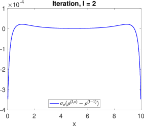
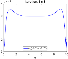
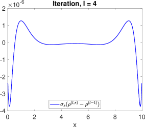
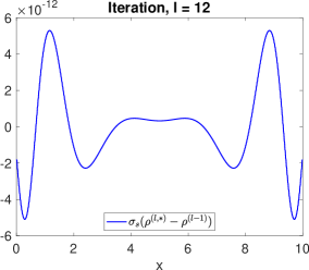
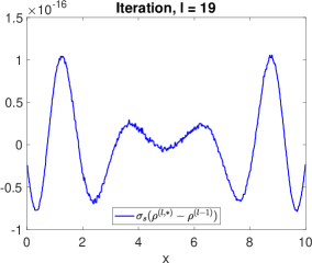
Figure 1: The source term in the correction equation for the $l$-th ($l=1,2,3,4,12,19$) iteration in the SI-DSA solving the problem in Sec. 3.2.1.

3.2.2 Two ROM based SA strategies

We design a ROM-based SA strategy (ROMSA) and a hybridized strategy called ROMSAD, which combines ROMSA and DSA.

ROMSA: If the underlying ROM is generated with a window size $\mathfrak{w}$, we call our SA strategy, ROMSA-$\mathfrak{w}$. ROMSA uses a ROM-based low rank approximation to the kinetic correction equation (14). Specifically, after the $l$-th source iteration, ROMSA solves the reduced order kinetic correction equation (27) to get the density correction $\delta\boldsymbol{\rho}^{{\boldsymbol{\mu}},(l)}=\delta\mathbf{U}_{r_{c}}^{\rho}\delta\mathbf{c}^{(l)}_{{\boldsymbol{\mu}},r_{c}}$, where $\mathbf{c}^{(l)}_{{\boldsymbol{\mu}},r_{c}}$ is the solution of (27). This ROM-based low rank approximation directly builds on the kinetic description of the correction equation and leverages low rank structures with respect to the parameters of the underlying parametric problem.

Numerically, we observe that ROMSA-$\mathfrak{w}$ achieves greater acceleration than DSA in the early stage of SISA. However, as iterations continue, the shapes of the source terms in the correction equations may vary significantly. With a moderate window size $\mathfrak{w}$, the underlying ROM may fail to accurately approximate the kinetic correction equation in the later stage of SISA. Consequently, ROMSA may suffer from an efficiency reduction in the later stage. For a clear illustration, in Fig. 2, we present how the difference of $\boldsymbol{\rho}$ for successive iterations, $||\boldsymbol{\rho}^{(k,*)}-\boldsymbol{\rho}^{(k-1)}||_{\infty}$, evolves for the cross-regime problem in Sec. 4.1.1. We observe a rapid decrease in $||\boldsymbol{\rho}^{(k,*)}-\boldsymbol{\rho}^{(k-1)}||_{\infty}$ for ROMSA-$3$ in the first $4$ iterations, followed by a slow decline starting from the $5$-th iteration. The decrease rate of $||\boldsymbol{\rho}^{(k,*)}-\boldsymbol{\rho}^{(k-1)}||_{\infty}$ for DSA is slower than or comparable to the rate for ROMSA in the first $4$ iterations, but becomes faster than ROMSA from the $5$-th iteration and onward.

In summary, with a moderate window size $\mathfrak{w}$, ROMSA is more efficient than DSA in the first few iterations of SISA, but less robust than DSA. Hence, we should only use ROMSA in the early stage when it is more efficient, and then switch to DSA to avoid the potential efficiency reduction of ROMSA.

Remark 3.2.

In our numerical tests, we observe that, for some parametric problems, SI accelerated by ROMSA converges very fast and does not suffer from the efficiency decline. Nevertheless, the lack of robustness severely restricts the applicability of ROMSA for general parametric problems. In contrary, DSA is robust for all tests.

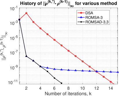
Figure 2: The history of the change of $\boldsymbol{\rho}$ in the $k$-th iteration, i.e. $||\boldsymbol{\rho}^{(k,*)}-\boldsymbol{\rho}^{(k-1)}||_{\infty}$, for the cross-regime problem in Sec. 4.1.1 with $\mu_{s}=19.772$ and $\epsilon_{\textrm{POD}}=10^{-9}$.

ROMSA hybridized with DSA (ROMSAD): To leverage high efficiency of ROMSA in the early stage of SISA and the robustness of DSA, we propose a hybridized strategy called ROMSAD.

As observed in Fig. 2, ROMSA is highly efficient in the early stage of SISA, while DSA maintains robust across all stages. We propose to use ROMSA in the first few iterations, and then automatically switch to DSA to avoid the potential efficiency reduction of ROMSA. Specifically, we use ROMSA after the $l$-th source iteration if

$$||\rho^{(l,*)}-\rho^{(l-1)}||_{\infty}\geq\epsilon_{\textrm{ROMSAD}}\quad\text{and}\quad l\leq\theta.$$

Otherwise, we use DSA. We choose

$$\epsilon_{\textrm{ROMSAD}}=\eta\max(\epsilon_{\textrm{SISA}}^{\textrm{train}},\epsilon_{\textrm{POD}}),\quad\eta\geq 0,$$ (28)

where $\epsilon_{\textrm{SISA}}^{\textrm{train}}$ is the tolerance in the stopping criteria of SISA generating our training data and $\epsilon_{\textrm{POD}}$ is the truncation tolerance in POD (see equation (20)). These two values determine the accuracy of the ROM utilized by ROMSA. We summarize our ROMSAD algorithm in Alg. 2. We refer to ROMSAD as ROMSAD-$\mathfrak{w},\theta$, when the underlying ROM is generated with a window size $\mathfrak{w}$, and ROMSA is allowed to be applied after at most the first $\theta$ source iterations. We denote SI with ROMSAD as SI-ROMSAD.

To demonstrate the effectiveness of ROMSAD, in Fig. 2, we also show how $||\boldsymbol{\rho}^{(k,*)}-\boldsymbol{\rho}^{(k-1)}||_{\infty}$ evolves for ROMSAD-$3,3$. ROMSAD-$3,3$ corrects the density with ROMSA after the first $3$ source iterations, and then switches to DSA. As a result, ROMSAD enjoys a decrease of $||\boldsymbol{\rho}^{(k,*)}-\boldsymbol{\rho}^{(k-1)}||_{\infty}$ as rapid as ROMSA in the first $4$ iterations, and thereafter demonstrates performance as robust as DSA. For this problem, overall, ROMSAD converges faster than both ROMSA and DSA. ROMSAD resolves the robustness issue of ROMSA without sacrificing its great efficiency in the early stage of SISA.

Algorithm 2 Determine applying ROMSA or DSA after the $l$-th source iteration of SI-ROMSAD.

  Input: current number of iterations $l$, a window size $\theta$, and a tolerance $\epsilon_{\textrm{ROMSAD}}$.

  if $1\leq l\leq\theta$ and $||\rho^{(l,*)}-\rho^{(l-1)}||_{\infty}\geq\epsilon_{\textrm{ROMSAD}}$, then

     apply ROMSA.

  else

     apply DSA.

  end if

Remark 3.3.

At first glance, it seems to be natural to directly use a ROM-based initial guess (ROMIG) for SI-ROMSAD. However, when using a ROMIG close to the exact solution, the shapes of source terms in the correction equations can differ significantly from those for other initial guesses, even in the early stage of SISA. Consequently, the underlying ROM of ROMSAD may not be accurate, unless it is built based on training data generated with the ROMIG.

A potential solution is to employ an iterative offline stage that adaptively updates ROMs for the parametric problem and the kinetic correction equation. Specifically, we first build an initial ROM for the parametric problem and then use an initial guess based on this ROM to generate training data for building an initial ROM for the correction equation. After initializing these ROMs, we can adaptively update them in an alternating manner. This iterative offline strategy will be left for future investigation.

4 Numerical results

In our numerical tests, we consider both 1D slab geometry and 2D $X$-$Y$ geometry. We compare the performance of the proposed DSA-ROMIG, ROMSA and ROMSAD to DSA using a zero initial guess. Throughout this section, we abbreviate DSA with a zero initial guess as DSA-$0$, ROMSA-$\mathfrak{w}$ as SA-$\mathfrak{w}$ and ROMSAD-$\mathfrak{w},\theta$ as SAD-$\mathfrak{w},\theta$. We denote SI with DSA as SI-DSA. SI-ROMSA and SI-ROMSAD have similar meanings. All the ROMs are constructed based on training data generated by DSA-$0$. SI-ROMSA and SI-ROMSAD always start with a $0$ initial guess.

For the choice of DSA, we use a consistent strategy following [47, 5]. In 1D slab geometry, the resulting diffusion equation is solved by a direct solver. In 2D $X$-$Y$ geometry, the diffusion equation is solved by an algebraic multigrid (AMG) solver implemented based on the iFEM package [48]. The reduced order kinetic correction problem for ROMSA is always solved by a direct solver, as its size is small.

In all examples, we use linear upwind DG spatial discretization $(K=1$ in (4)). We set $\eta$ as $\eta=0.1$ in the threshold of the switching criteria of ROMSAD (see (28)). We refer to the training set for parameters as $\mathcal{P}_{\textrm{train}}$, and the test set for parameters as $\mathcal{P}_{\textrm{test}}$. The training set and the test set satisfy $\mathcal{P}_{\textrm{train}}\cap\mathcal{P}_{\textrm{test}}=\emptyset$.

Recall that we denote the tolerance in the stopping criteria of SISA as $\epsilon_{\textrm{SISA}}$, the truncation tolerance to POD basis in (20) as $\epsilon_{\textrm{POD}}$, and the window size to assemble the snapshot matrix for the correction equation as $\mathfrak{w}$. We define the average number of iterations for the test set as

$$n_{\textrm{iter}}=\frac{\sum_{{\boldsymbol{\mu}}\in\mathcal{P}_{\textrm{train}}}\textrm{number of iterations for the convergence for the parameter}{\boldsymbol{\mu}}}{\textrm{total number of parameters in }\mathcal{P}_{\textrm{test}}}.$$

Similarly, we define the average relative computational time with respect to DSA-$0$ as $T_{\textrm{rel}}$. To verify that SI-DSA-ROMIG, SI-ROMSA and SI-ROMSAD converge to the correct solutions, we use solutions given by SI-DSA -$0$ as the reference solutions. We define the average derivation from the reference solutions as

$$\mathcal{D}_{\infty}^{\rho}=\frac{\sum_{{\boldsymbol{\mu}}\in\mathcal{P}_{\textrm{train}}}||\boldsymbol{\rho}_{\boldsymbol{\mu}}^{\textrm{test}}-\boldsymbol{\rho}^{\textrm{DSA}}_{{\boldsymbol{\mu}}}||_{\infty}}{\textrm{total number of parameters in }\mathcal{P}_{\textrm{test}}},$$

where $\boldsymbol{\rho}_{{\boldsymbol{\mu}}}^{\textrm{test}}$ is obtained by the method under consideration.

4.1 1D slab geometry

In our tests for 1D slab geometry, $16$ Gauss-Legendre quadrature points for $[-1,1]$ is used for angular discretization.

4.1.1 Cross-regime problem

We consider a parametric problem with a spatially varying scattering cross section. The set-up of the problem is as follows:

$$\Omega_{\mathbf{x}}=[0,10],\;G=0.01,\;\sigma_{a}=0,\;\sigma_{s}(x)=0.1+\mu_{s}x,\;\;\sigma_{t}=\sigma_{a}+\sigma_{s},\;f(0,\xi)=0\;\text{with }\xi>0,\;f(10,\xi)=0\;\text{with }\xi<0.$$

The slope of the linear scattering cross section $\mu_{s}\in[10,20]$ is the parameter of this problem. We use a uniform mesh with $N_{\mathbf{x}}=400$ to partition the computational domain. The tolerance in the stopping criteria of SISA is set to $\epsilon_{\textrm{SISA}}=10^{-11}$.

As we move from the left to the right of the computational domain, the scattering cross section $\sigma_{s}(x)$ continuously changes from $0.1$ to $0.1+10\mu_{s}$ which is bigger than $100$ for $\mu_{s}\in[10,20]$. In other words, there is a smooth transition in the material property from transport dominance to scattering dominance. The slope $\mu_{s}$ determines how fast this transition is.

The training set $\mathcal{P}_{\textrm{train}}=\{\mu_{s,j}=10+j\Delta\mu,\;\Delta\mu=\frac{1}{4},\;j=0,\dots,40\}$ consists of $41$ uniformly distributed samples in $[10,20]$. To test the performance of the proposed methods, we randomly sample $20$ different values of $\mu_{s}$ from $[10,20]$. Solutions corresponding to $3$ test samples are presented in the left picture of Fig. 3. Using this cross-regime problem, we investigate the influence of the POD truncation tolerance $\epsilon_{\textrm{POD}}$ and the window size $\mathfrak{w}$ on the performance of DSA-ROMIG, ROMSA and ROMSAD.

Dimensions of the reduced order spaces in our ROMs for the parametric problem ($r_{p}$) and the corresponding kinetic correction equations ($r_{c}$) are displayed in Tab. 1. With the same truncation tolerance $\epsilon_{\textrm{POD}}$, We observe that $r_{p}$ is always not greater than $r_{c}$. In addition, for the same tolerance $\epsilon_{\textrm{POD}}$, the dimension of the reduced order space for the correction equation, $r_{c}$, grows as the window size $\mathfrak{w}$ increases.

In Tab. 2, we compare the performance of various methods. Key observations are as follows.

1. Influence of the POD truncation tolerance $\epsilon_{\textrm{POD}}$: For this problem, the performance of DSA-ROMIG is insensitive to the choice of the tolerance $\epsilon_{\textrm{POD}}$, and it converges with nearly $60\%$ of iterations with respect to DSA-$0$.

   ROMSA is sensitive to the choice of the tolerance $\epsilon_{\textrm{POD}}$ for this problem. With $\epsilon_{\textrm{POD}}=10^{-9}$, ROMSA needs even more iterations for convergence than DSA-$0$, regardless of the window size $\mathfrak{w}$. The results for ROMSA-$1$ are identical with $\epsilon_{\textrm{POD}}=10^{-9}$ and $\epsilon_{\textrm{POD}}=10^{-10}$, as the underlying reduced order spaces are the same. When $\epsilon_{\textrm{POD}}=10^{-11}$, ROMSA-$1$ converges with $47\%$ number of iterations with respect to DSA-$0$. For $\epsilon_{\textrm{POD}}=10^{-10}$ and $\epsilon_{\textrm{POD}}=10^{-11}$, ROMSA-$3$ and ROMSA-$5$ result in convergence faster than DSA, regardless of whether the zero or the ROM-based initial guess is used.

   ROMSAD is more robust than ROMSA concerning the choice of the tolerance $\epsilon_{\textrm{POD}}$. Compared with DSA-$0$ and DSA-ROMIG, ROMSAD consistently achieves greater acceleration, regardless of the window size $\mathfrak{w}$. Due to its robustness, ROMSAD-$\mathfrak{w},3$ is significantly more efficient than ROMSA-$\mathfrak{w}$ for $\epsilon_{\textrm{POD}}=10^{-9}$ and $\epsilon_{\textrm{POD}}=10^{-10}$. When $\epsilon_{\textrm{POD}}=10^{-11}$, the underlying ROM for the correction equation becomes accurate, and ROMSAD-$\mathfrak{w},3$ is slightly more efficient than ROMSA-$\mathfrak{w}$.

2. Influence of $\mathfrak{w}$ on ROMSAD: When $\epsilon_{\textrm{POD}}=10^{-9}$, ROMSAD-$\mathfrak{w},3$ converges with a comparable number of iterations for window sizes $\mathfrak{w}=1,3,5$. When $\epsilon_{\textrm{POD}}=10^{-10}$ or $10^{-11}$, ROMSAD converges faster if the underlying ROM is generated with a wider window size $\mathfrak{w}$.

3. We observe that the average relative computational time with respect to DSA-$0$ is approximately proportional to the average number of iterations for DSA-ROMIG, but not to that number for ROMSA and ROMSAD. The reason is as follows. In 1D slab geometry, we only use $16$ quadrature points in our angular discretization. As a result, the computational time of solving the diffusion equation in the correction step of DSA is not negligible compared to the time for the source iteration step. In contrast, the computational time for solving the low-dimensional reduced order problem in the correction step of ROMSA is almost negligible compared to the time for the source iteration.

   In higher dimensions, a large number of angular directions are required. As a result, the computational cost of the correction step is negligible in comparison with the source iteration step, no matter we use DSA or ROMSA. Therefore, the relative computational times for DSA, ROMSA and ROMSAD should be all approximately proportional to the number of iterations in higher dimensions.

For this problem, ROMSAD and DSA-ROMIG are more robust than ROMSA, and more efficient than DSA-$0$. In the rest of the numerical section, we will mainly focus on comparing these two methods with DSA-$0$.

$\epsilon_{\textrm{POD}}$	$r_{p}$	$r_{c}$ with $\mathfrak{w}=1$	$r_{c}$ with $\mathfrak{w}=3$	$r_{c}$ with $\mathfrak{w}=5$
$10^{-9}$	$6$	$6$	$15$	$24$
$10^{-10}$	$6$	$6$	$18$	$29$
$10^{-11}$	$7$	$7$	$21$	$34$
$10^{-12}$	$9$	$9$	$26$	$42$

Table 1: Dimensions of the reduced order spaces for the parametric problem ($r_{p}$) and the correction equation ($r_{c}$) for the cross-regime problem in Sec. 4.1.1 with different POD truncation tolerances $\epsilon_{\textrm{POD}}$.

	DSA-$0$	DSA-ROMIG	SA-$1$	SAD-$1,3$	SA-$3$	SAD-$3,3$	SA-$5$	SAD-$5,3$
${n}_{\textrm{iter}}$	15	9	23.75	6.55	42.25	6.85	72.95	6.95
${T}_{\textrm{rel}}$	100%	58.801%	104.552%	31.544%	186.234%	32.612%	321.982%	33.063%
${\mathcal{D}}^{\rho}_{\infty}$	N.A.	4.15e-11	6.74e-9	5.06e-11	5.23e-9	5.48e-11	3.18e-9	4.67e-11

(a) $\epsilon_{\textrm{POD}}=10^{-9}$, $\epsilon_{\textrm{SISA}}=10^{-11}$

	DSA-$0$	DSA-ROMIG	SA-$1$	SAD-$1,3$	SA-$3$	SAD-$3,3$	SA-$5$	SAD-$5,3$
${n}_{\textrm{iter}}$	15	9	23.75	6.6	12.05	5.8	8.6	5.25
${T}_{\textrm{rel}}$	100%	58.801%	101.405%	29.681%	52.911%	29.710%	37.806%	26.146%
${\mathcal{D}}^{\rho}_{\infty}$	N.A.	4.15e-11	6.74e-9	5.05e-11	1.00e-9	4.15e-11	2.53e-9	4.78e-11

(b) $\epsilon_{\textrm{POD}}=10^{-10}$, $\epsilon_{\textrm{SISA}}=10^{-11}$

	DSA-$0$	DSA-ROMIG	SA-$1$	SAD-$1,3$	SA-$3$	SAD-$3,3$	SA-$5$	SAD-$5,3$
${n}_{\textrm{iter}}$	15	9	7.05	5.65	4.55	4.5	3.7	3.7
${T}_{\textrm{rel}}$	100%	58.722%	30.669%	28.650%	20.013%	21.216%	16.342%	16.425%
${\mathcal{D}}^{\rho}_{\infty}$	N.A.	3.68e-11	2.37e-9	5.31e-11	6.24e-10	2.31e-10	8.58e-10	8.05e-10

(c) $\epsilon_{\textrm{POD}}=10^{-11}$, $\epsilon_{\textrm{SISA}}=10^{-11}$

Table 2: Results for the cross-regime problem in 1D slab geometry (see Sec. 4.1.1).

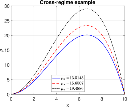
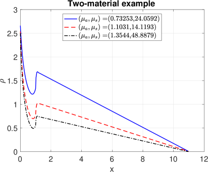
Figure 3: Reference solutions for $3$ samples in the test set. Left: the cross-regime example in Sec. 4.1.1. Right: the two-material example in Sec. 4.1.2.

4.1.2 Two-material problem

We consider a parametric two-material problem with the following set-up:

$$\Omega_{\mathbf{x}}=[0,11],\;G=0,\;\sigma_{a}(x)=\begin{cases}\mu_{a},\;0<x\leq 1,\\ 0,\;1<x<11,\end{cases}\;\sigma_{s}(x)=\begin{cases}0,\;0<x\leq 1,\\ \mu_{s},\;1<x<11,\end{cases}\;\sigma_{t}(x)=\sigma_{a}(x)+\sigma_{s}(x),$$

$$f(0,\xi)=5\;\text{with }\xi>0,\;f(11,\xi)=0\;\text{with }\xi<0.$$

There is a pure absorption region ($[0,1]$) and a pure scattering region ($[1,11]$) in the computational domain. Parameters $\mu_{a}\in[0.5,1.5]$ and $\mu_{s}\in[10,50]$ are the strength of the absorption and scattering cross sections in the absorption and scattering regions, respectively. A non-uniform mesh with $\Delta x=\Delta x_{1}=\frac{1}{100}$ on $[0,1]$ and $\Delta x=\Delta x_{2}=\frac{1}{10}$ on $[1,11]$ is used to partition the computational domain. The tolerance in the stopping criteria of SISA is set to $\epsilon_{\textrm{SISA}}=10^{-12}$.

The training set for this problem is

$$\mathcal{P}_{\textrm{train}}=\{(\mu_{a,m},\mu_{s,n}):\;\mu_{a,m}=0.5+0.1m,\;\mu_{s,n}=10+n,0\leq m\leq 10,0\leq n\leq 40\}.$$

To test the performance of the proposed methods, we randomly sample $20$ pairs of $(\mu_{a},\mu_{s})$ from $[0.5,1.5]\times[10,50]$. Solutions corresponding to $3$ samples in the test set are presented in the right picture of Fig. 3.

The results are summarized in Tab. 3. With $\theta=1,2,3$, i.e. the maximum number of iterations allowed to use ROMSA in ROMSAD, ROMSAD-$\mathfrak{w},\theta$ turn out to have identical performance for this problem, when the same window size $\mathfrak{w}$ ($\mathfrak{w}=3,5$) is applied. With the POD truncation tolerances $\epsilon_{\textrm{POD}}=10^{-6}$, $10^{-9}$ and $10^{-10}$, both DSA-ROMIG and ROMSAD leads to convergence faster than DSA-$0$. The efficiency of DSA-ROMIG and ROMSAD improves, as we decrease the tolerance $\epsilon_{\textrm{POD}}$. For this example, DSA-ROMIG is slightly more efficient than ROMSAD, when their underlying ROMs are generated with the same tolerance $\epsilon_{\textrm{POD}}$.

	$\epsilon_{\textrm{POD}}$	DSA-$0$	DSA-ROMIG	SAD-$3,\theta$	SAD-$5,\theta$
$n_{\textrm{iter}}$	$10^{-6}$	14.6	8.1	8.9	9.05
$T_{\textrm{rel}}$		100%	54.01%	55.78%	56.68%
$\mathcal{D}_{\infty}^{\rho}$		N.A.	1.14e-12	1.40e-12	1.33e-12
$n_{\textrm{iter}}$	$10^{-9}$	14.6	4.2	5.35	5.35
$T_{\textrm{rel}}$		100%	27.85%	33.16%	33.16%
$\mathcal{D}_{\infty}^{\rho}$		N.A.	9.31e-13	1.19e-12	1.09e-12
$n_{\textrm{iter}}$	$10^{-10}$	14.6	3.35	4.25	4.25
$T_{\textrm{rel}}$		100%	22.09%	26.50%	26.31%
$\mathcal{D}_{\infty}^{\rho}$		N.A.	1.12e-12	1.17e-12	1.07e-12

Table 3: Results for the two-material problem in Sec. 4.1.2. The most number of iterations applying ROMSA in ROMSAD is $\theta=1,3,5$. Performance of SAD-$3,\theta$ and SAD-$5,\theta$ are identical to each other. Dimensions of the reduced order spaces: when $\epsilon_{\textrm{POD}}=10^{-6}$, $r_{p}=21$, $r_{c}=49$ for $\mathfrak{w}=3$ and $r_{c}=54$ for $\mathfrak{w}=5$; when $\epsilon_{\textrm{POD}}=10^{-9}$, $r_{p}=44$, $r_{c}=101$ for $\mathfrak{w}=3$ and $r_{c}=120$ for $\mathfrak{w}=5$; when $\epsilon_{\textrm{POD}}=10^{-10}$, $r_{p}=53$, $r_{c}=123$ for $\mathfrak{w}=3$ and $r_{c}=147$ for $\mathfrak{w}=5$.

4.2 2D $X$-$Y$ geometry and $\mathbb{S}^{2}$ as angular space

To further demonstrate the performance of our methods, we consider a sires of problems in 2D $X$-$Y$ geometry with $\mathbb{S}^{2}$ as the angular space. For the $S_{N}$ angular discretization, we use the CL($N_{\phi}$,$N_{v_{z}}$) quadrature rule, which is the tensor product of the normalized $N_{\phi}$-points Chebyshev quadrature rule for the unit circle and the normalized $N_{v_{z}}$-points Gauss-Legendre quadrature rule for $v_{z}\in[-1,1]$.

4.2.1 Homogeneous medium

We consider a parametric problem with zero inflow boundary conditions and a homogeneous background medium:

$$\Omega_{\mathbf{x}}=[0,1]^{2},\;G(x,y)=\exp(-100((x-0.5)^{2}+(y-0.5)^{2})),\;\sigma_{a}(\mathbf{x})=0,\;\sigma_{s}(\mathbf{x})=\mu_{s},\;\mu_{s}\in[0.9,1.1].$$

We use an $80\times 80$ uniform rectangular mesh to partition $\Omega_{\mathbf{x}}$ and the CL-($30,6$) quadrature rule to discretize the angular space. The tolerance in the stopping criteria of SISA is set to $\epsilon_{\textrm{SISA}}=10^{-12}$.

For this problem, we construct our ROMs using a uniformly sampled training set with $21$ samples: $\mathcal{P}_{\textrm{train}}=\{\mu_{s,m}=0.9+m\Delta\mu,\;\Delta\mu=\frac{1}{200},0\leq m\leq 20\}$. We test the performance of the proposed methods with $10$ randomly sampled values of $\mu_{s}$ from $[0.9,1.1]$. POD basis is generated with the tolerance $\epsilon_{\textrm{POD}}=10^{-9}$. The solution for the test sample $\mu_{s}=1.0101$ is presented in Figure 4.

Results for the test set are summarized in Tab. 4. Using DSA-ROMIG, SI converges with approximately $19.8\%$ computational time and $20.5\%$ number of iterations compared to DSA-$0$. Using ROMSA-$3$ and ROMSAD-$3,3$, SI converges with slightly less than $20\%$ computational time and number of iterations compared to DSA-$0$. Unlike 1D slab geometry, the relative computational time is approximately proportional to the number of iterations for convergence. The reason why is as follows. In one source iteration, $180$ block lower triangular linear systems are solved with transport sweep, while only one diffusion or reduced order system is solved in one correction step. Therefore, the computational costs of the correction step for both DSA and ROMSA are almost negligible in comparison with the source iteration step.

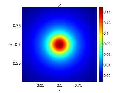
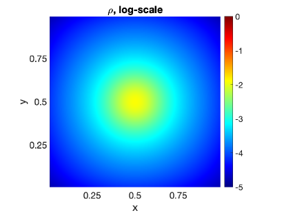
Figure 4: The reference solution for the homogeneous medium problem in Sec. 4.2.1 with $\mu_{s}=1.0101$. The right figure is the solution under log-scale.

	DSA-$0$	DSA-ROMIG	SA-$3$	SAD-$3,3$
${n}_{\textrm{iter}}$	14.6	3.0	2.9	2.9
${T}_{\textrm{rel}}$	100%	19.826%	16.523%	17.736%
${\mathcal{D}}^{\rho}_{\infty}$	N.A.	2.46e-13	2.64e-13	2.16e-13

Table 4: Results for the problem with homogeneous medium in Sec. 4.2.1. Dimensions of reduced order spaces: $r_{p}=5$ and $r_{c}=14$.

4.2.2 Lattice problem

We consider a parametric lattice problem with zero inflow boundary conditions in the computational domain $\Omega_{\mathbf{x}}=[0,5]^{2}$. The geometry set-up is presented in the left picture of Fig. 5. In Fig. 5, black regions are pure absorption regions with $(\sigma_{a},\sigma_{s})=(\mu_{a},0)$. Other regions are pure scattering regions with $(\sigma_{a},\sigma_{s})=(0,\mu_{s})$. The parameter ${\boldsymbol{\mu}}=(\mu_{a},\mu_{s})\in[95,105]\times[0.5,1.5]$ determines the strength of absorption in the pure absorption region and the strength of scattering in the pure scattering region. The source term

$$G(x,y)=\begin{cases}1.0,\quad\text{if}\quad|x-2.5|<0.5\;\text{and}\quad|y-2.5|<0.5,\\ 0,\quad\text{otherwise},\end{cases}$$

is imposed in the orange region. We use a uniform mesh with $50\times 50$ elements to partition the computational domain and discretize the angular space with the CL($40,6$) quadrature rule. The tolerance for the SISA stopping criteria is set to $\epsilon_{\textrm{SISA}}=10^{-12}$.

The training set

$$\mathcal{P}_{\textrm{train}}=\{(\mu_{a},\mu_{s})=(95+i\Delta\mu_{a},0.5+0.1j\Delta\mu_{s}),\Delta\mu_{a}=1,\Delta\mu_{s}=0.1,i,j=0,1,\dots,10\}$$

has $121$ pairs of uniformly sampled $(\mu_{a},\mu_{s})$ in total. We test the performance of our methods with $10$ randomly sampled $(\mu_{a},\mu_{s})$ from $[95,105]\times[0.5,1.5]$. A reference solution corresponding to a test sample is presented in the right picture of Fig. 5.

Results for parameters in the test set are summarized in Tab. 5. Various POD truncation tolerances are applied to generate ROMs. When $\epsilon_{\textrm{POD}}=10^{-9}$, DSA-ROMIG is approximately $1.6$ times as fast as ROMSAD-$3,5$ and $4$ times as fast as DSA-$0$. When $\epsilon_{\textrm{POD}}=10^{-10}$, DSA-ROMIG and ROMSAD-$3,5$ have comparable speeds, leading to a nearly $5$ times acceleration compared to DSA-$0$. When $\epsilon_{\textrm{POD}}=10^{-11}$, ROMSAD-$3,5$ becomes the fastest and leads to a convergence with approximately $11.41\%$ computational time and $12.69\%$ number of iterations compared to DSA-$0$. Overall, for this example, as the POD truncation tolerance $\epsilon_{\textrm{POD}}$ decreases, both of DSA-ROMIG and ROMSAD-$3,5$ gain performance boosts, while the boost gained by ROMSAD-$3,5$ is larger. When ROMs are generated using a larger tolerance $\epsilon_{\textrm{POD}}$, DSA-ROMIG outperforms ROMSAD-$3,5$. On the other hand, ROMSAD-$3,5$ is faster for a smaller tolerance $\epsilon_{\textrm{POD}}$.

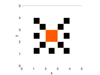
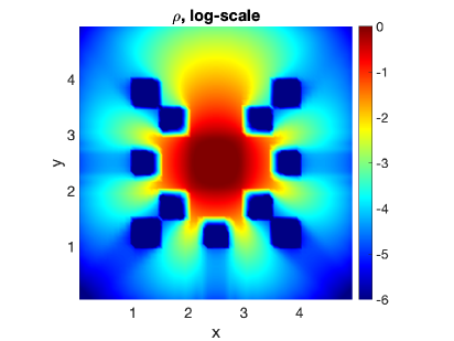
Figure 5: The set-up and a reference solution for the lattice problem in Sec. 4.2.2. Left: the set-up for the lattice problem. Black: pure absorption regions with $(\sigma_{a},\sigma_{s})=(\mu_{a},0)$. White and orange: pure scattering regions with $(\sigma_{a},\sigma_{s})=(0,\mu_{s})$. Orange: constant source term with $G=1$. Right: the reference solution under log-scale for $(\mu_{a},\mu_{s})=(97.235,1.051)$.

	$\epsilon_{\textrm{POD}}$	DSA-$0$	DSA-ROMIG	SAD-$3,5$
$n_{\textrm{iter}}$	$10^{-9}$	19.7	5.1	8.0
$T_{\textrm{rel}}$		100%	25.592%	39.498%
$\mathcal{D}_{\infty}^{\rho}$		N.A.	6.29e-13	1.30e-12
$n_{\textrm{iter}}$	$10^{-10}$	19.7	3.9	4.2
$T_{\textrm{rel}}$		100%	19.561%	20.213%
$\mathcal{D}_{\infty}^{\rho}$		N.A.	4.83e-13	6.48e-13
$n_{\textrm{iter}}$	$10^{-11}$	19.7	3.5	2.5
$T_{\textrm{rel}}$		100%	17.419%	11.407%
$\mathcal{D}_{\infty}^{\rho}$		N.A.	4.96e-13	6.39e-13

Table 5: Results for the lattice problem in Sec. 4.2.2. Dimensions of the reduced order spaces: $r_{p}=25$ and $r_{c}=66$ for $\epsilon_{\textrm{POD}}=10^{-9}$; $r_{p}=29$ and $r_{c}=80$ for $\epsilon_{\textrm{POD}}=10^{-10}$; $r_{p}=34$ and $r_{c}=96$ for $\epsilon_{\textrm{POD}}=10^{-11}$.

4.2.3 Pin-cell problem

We consider a parametric pin-cell problem with zero inflow boundary conditions and the geometric set-up in the top left picture of Fig. 6. The computational domain is $\Omega_{\mathbf{x}}=[-1,1]^{2}$ and the source is $G(x,y)=\exp(-100(x^{2}+y^{2}))$. The absorption and scattering cross sections are

$$\sigma_{a}(x,y)=\begin{cases}\mu_{a},\;\text{if}\;|x|\leq 0.5\;\text{and}\;|y|\leq 0.5,\\ 0,\;\text{otherwise},\end{cases}\;\text{and}\quad\sigma_{s}(x,y)=\begin{cases}\mu_{s},\;\text{if}\;|x|\leq 0.5\;\text{and}\;|y|\leq 0.5,\\ 100,\;\text{otherwise}.\end{cases}$$

Parameters $\mu_{a}\in[0.05,0.5]$ and $\mu_{s}\in[0.05,0.5]$ are the absorption and scattering cross sections for the inner cell, respectively. As we move from the center of the computational domain to the outer part, there is a sharp transition in the strength of the scattering effect from weak to strong. The computational domain is partitioned with an $80\times 80$ uniform mesh. We use the CL($30,6$) quadrature rule for the angular discretization. The tolerance in the stopping criteria for SISA is set to $\epsilon_{\textrm{SISA}}=10^{-11}$.

To build ROMs, we use a training set with $25$ uniformly distributed samples:

$$\mathcal{P}_{\textrm{train}}=\{(\mu_{a},\mu_{s})=(i\Delta\mu_{a},j\Delta\mu_{s}),\;i,j=1,\dots 5,\;\Delta\mu_{a}=\Delta\mu_{s}=0.05\}.$$

We generate our ROMs with the tolerance $\epsilon_{\textrm{POD}}=10^{-9}$. To test the performance of our methods, we randomly sample $10$ pairs of $(\mu_{a},\mu_{s})$ from $[0.05,0.5]^{2}$. Solutions for $3$ pairs of test samples are presented in Fig. 6. When the difference between material properties of the inner and outer parts of the computational domain is larger, the density has sharper features near the material interface.

The performance of various methods is demonstrated in Tab. 6. Due to the significant jump in $\sigma_{s}$ near the material interface, this problem is challenging for SISA. On average, SISA using DSA-$0$ needs $39.3$ iterations to converge. Both of DSA-ROMIG and ROMSAD-$3,5$ significantly accelerate the convergence of SISA. DSA-ROMIG leads to approximately $7.4$ times the acceleration compared to DSA-$0$. ROMSAD-$3,5$ results in nearly $10$ times the acceleration compared to DSA-$0$.

In Fig. 7, we show how the change of the density in the $k$-th source iteration, $||\boldsymbol{\rho}^{(k,*)}-\boldsymbol{\rho}^{(k-1)}||_{\infty}$, evolves for various methods. Due to the use of a ROM-based initial guess, DSA-ROMIG starts from a small initial difference $||\boldsymbol{\rho}^{(1,*)}-\boldsymbol{\rho}^{0}||_{\infty}$, and converges earlier than DSA-$0$. The decreasing rates for DSA-ROMIG and DSA-$0$ appear similar to each other. ROMSAD-$3,5$ starts from a zero initial guess, so $||\boldsymbol{\rho}^{(1,*)}-\boldsymbol{\rho}^{(0)}||_{\infty}$ are the same for ROMSAD-$3,5$ and DSA-$0$. Leveraging a reduced order kinetic correction equation, $||\boldsymbol{\rho}^{(k,*)}-\boldsymbol{\rho}^{(k-1)}||_{\infty}$ for ROMSAD-$3,5$ drops significantly in the second iteration, and its decline rate is faster than DSA in the third iteration. In fact, for the presented test sample, SI-ROMSAD-$3,5$ converges with only $3$ iterations.

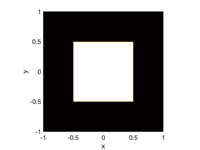
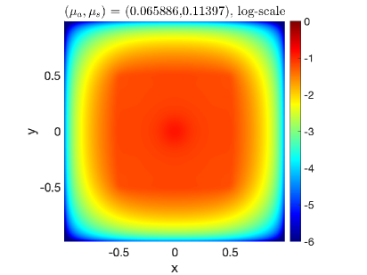
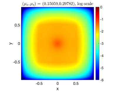
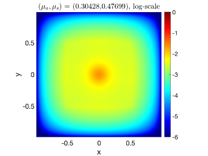
Figure 6: The set-up and reference solutions for the pin-cell problem in Sec. 4.2.3. Top left: problem set-up. Other pictures: $\rho$ for various pairs of parameters $(\mu_{s},\mu_{a})$ (under log-scale).

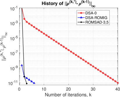
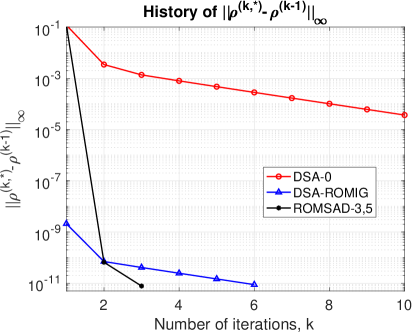
Figure 7: The history of the change of $\boldsymbol{\rho}$ in the $k$-th iteration, i.e. $||\boldsymbol{\rho}^{(k,*)}-\boldsymbol{\rho}^{(k-1)}||_{\infty}$, for the pin-cell problem in Sec. 4.2.3 with $(\mu_{a},\mu_{s})=(0.15068,0.2978)$. Left: entire history. Right: zoomed-in picture.

	DSA-$0$	DSA-ROMIG	SAD-$3,5$
${n}_{\textrm{iter}}$	39.3	5.3	4
${T}_{\textrm{rel}}$	100%	13.011%	9.013%
${\mathcal{D}}^{\rho}_{\infty}$	N.A.	2.34e-11	8.93e-11

Table 6: Results for the pin-cell problem in Sec. 4.2.3. Dimensions of the reduced order spaces: $r_{p}=21$ and $r_{c}=59$.

4.2.4 Variable scattering cross section

We consider a parametric problem on the computational domain $\Omega_{\mathbf{x}}=[-1,1]^{2}$ with zero inflow boundary conditions and a variable scattering cross section

$$\sigma_{s}(x,y)=\begin{cases}\mu_{s}r^{4}(2-r^{2})^{2}+0.1,\quad r=\sqrt{x^{2}+y^{2}}\leq 1,\\ \mu_{s}+0.1,\quad\text{otherwise},\end{cases}\quad\mu_{s}\in[49.9,99.9],$$ (29)

and a zero absorption cross section. The scattering cross section $\sigma_{s}(\mathbf{x})$ with $\mu_{s}=99.9$ is presented in the left figure of Fig. 8. From the center of the computational domain to the outer part, the scattering cross section smoothly changes from $0.1$ to $\mu_{s}+0.1$ which is at least $50$ for $\mu_{s}\in[49.9,99.9]$. In other words, there is a smooth transition from transport dominance to scattering dominance. The parameter $\mu_{s}$ determines how fast $\sigma_{s}(\mathbf{x})$ changes. The source is $G(x,y)=\frac{10}{\pi}\exp(-100(x^{2}+y^{2})).$ We use an $80\times 80$ uniform mesh to partition the computation domain and the CL($30,6$) quadrature rule for the angular discretization. The tolerance in the stopping criteria of SISA is set to $\epsilon_{\textrm{SISA}}=10^{-12}$.

We use a training set with $50$ uniformly distributed samples and build ROMs with the POD truncation tolerance $\epsilon_{\textrm{POD}}=10^{-11}$. To test the performance of our methods, we randomly sample $10$ values of $\mu_{s}$ from $[49.9,99.9]$. Results for this test are summarized in Tab. 7. Compared with DSA-$0$, both DSA-ROMIG and ROMSAD-$3,5$ result in greater acceleration. DSA-ROMIG outperforms ROMSAD-$3,5$ for this example.

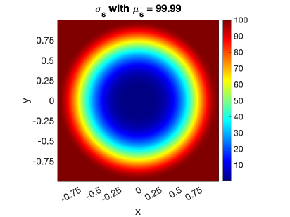
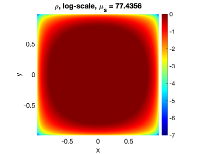
Figure 8: Left: $\sigma_{s}(\mathbf{x})$ with $\mu_{s}=99.9$ for the variable scattering probelm in Sec. 4.2.4. Right: $\rho$ for $\mu_{s}=77.4356$ (under log-scale).

	DSA-$0$	DSA-ROMIG	SAD-$3,5$
${n}_{\textrm{iter}}$	17	2.6	4.2
${T}_{\textrm{rel}}$	100%	14.288%	19.913%
${\mathcal{D}}^{\rho}_{\infty}$	N.A.	8.46e-13	5.71e-12

Table 7: Results for the variable scattering problem in Sec. 4.2.4. Dimensions of the reduced order spaces: $r_{p}=9$ and $r_{c}=18$.

5 Conclusion

We propose two strategies to utilize data-driven ROMs to enhance SISA for parametric RTE.

1. We use the ROM for the parametric problem to provide an improved initial guess for SI-DSA.

2. We exploit the ROM for the kinetic correction equation to design a new ROM-based synthetic acceleration strategy called ROMSA. We further combine ROMSA with DSA to develop a strategy named ROMSAD. ROMSAD leverages the high efficiency of ROMSA in the early stage of SISA and the robustness of DSA in the later stage. Additionally, we propose an approach to construct the ROM for the kinetic correction equation without directly solving it.

In our numerical tests, we observe that, compared with DSA using a $0$ initial guess, DSA-ROMIG and ROMSAD achieve greater acceleration. Specifically, DSA-ROMIG is more robust with respect to different choices of the POD truncation tolerance $\epsilon_{\textrm{POD}}$. ROMSAD has the potential to achieve rapid convergence for some challenging problems. For example, in a multiscale pin-cell problem, SI-ROMSAD achieves $10$ times the acceleration compared to SI-DSA with the same initial guess.

Potential future directions are as follows. First, as mentioned in Remark 3.3, we may not be able to directly use a ROM based initial guess for ROMSAD. An enhanced adaptive offline stage is required to leverage the power of both the ROMIG and ROMSAD. Second, to further improve the efficiency and robustness of ROMSAD, a switching strategy based on error estimators can be designed to determine when switching from ROMSA to DSA. Third, the offline cost of building ROMs can be reduced by using a greedy algorithm which identifies most representative parameters in the training set and computes full order solutions only for these parameters offline. Fourth, we plan to extend our method to parametric problems with anisotropic scattering, multiple energy groups and nonlinear terms. Moreover, we aim to integrate our method as a building block for uncertainty quantification, shape optimization, and solvers for inverse problems.

CRediT authorship contribution statement

Zhichao Peng: Writing – original draft, Writing – review & editing, Visualization, Validation, Software, Methodology, Data curation, Conceptualization.

Declaration of generative AI and AI-assisted technologies in the writing process

During the preparation of this work the author(s) used ChatGPT in order to check grammar errors and improve readability. After using this tool/service, the author(s) reviewed and edited the content as needed and take(s) full responsibility for the content of the publication.

References

- [1] S. R. Arridge, J. C. Schotland, Optical tomography: forward and inverse problems, Inverse problems 25 (12) (2009) 123010.
- [2] G. C. Pomraning, The equations of radiation hydrodynamics, International Series of Monographs in Natural Philosophy, Oxford: Pergamon Press (1973).
- [3] H.-T. Janka, K. Langanke, A. Marek, G. Martínez-Pinedo, B. Müller, Theory of core-collapse supernovae, Physics Reports 442 (1-6) (2007) 38–74.
- [4] R. Spurr, T. Kurosu, K. Chance, A linearized discrete ordinate radiative transfer model for atmospheric remote-sensing retrieval, Journal of Quantitative Spectroscopy and Radiative Transfer 68 (6) (2001) 689–735.
- [5] M. L. Adams, E. W. Larsen, Fast iterative methods for discrete-ordinates particle transport calculations, Progress in Nuclear Energy 40 (2002) 3–159.
- [6] H. Kopp, Synthetic method solution of the transport equation, Nuclear Science and Engineering 17 (1) (1963) 65–74.
- [7] R. Alcouffe, Dittusion Synthetic Acceleration Methods For the Diamond-Ditterenced Discrete-Ordinotes Equations, Nuclear science and engineering 64 (1977) 344–355.
- [8] M. L. Adams, W. R. Martin, Diffusion synthetic acceleration of discontinuous finite element transport iterations, Nuclear science and engineering 111 (2) (1992) 145–167.
- [9] T. Wareing, New diffusion-sythetic acceleration methods for the equations with corner balance spatial differencing (1993).
- [10] V. Y. Gol’din, A quasi-diffusion method of solving the kinetic equation, Zhurnal Vychislitel’noi Matematiki i Matematicheskoi Fiziki 4 (6) (1964) 1078–1087.
- [11] D. Y. Anistratov, V. Y. Gol’Din, Nonlinear methods for solving particle transport problems, Transport Theory and Statistical Physics 22 (2-3) (1993) 125–163.
- [12] S. Olivier, W. Pazner, T. S. Haut, B. C. Yee, A family of independent Variable Eddington Factor methods with efficient preconditioned iterative solvers, Journal of Computational Physics 473 (2023) 111747.
- [13] L. J. Lorence Jr, J. Morel, E. W. Larsen, An synthetic acceleration scheme for the one-dimensional sn equations with linear discontinuous spatial differencing, Nuclear Science and Engineering 101 (4) (1989) 341–351.
- [14] Y. Choi, P. Brown, W. Arrighi, R. Anderson, K. Huynh, Space–time reduced order model for large-scale linear dynamical systems with application to boltzmann transport problems, Journal of Computational Physics 424 (2021) 109845.
- [15] A. G. Buchan, A. Calloo, M. G. Goffin, S. Dargaville, F. Fang, C. C. Pain, I. M. Navon, A POD reduced order model for resolving angular direction in neutron/photon transport problems, Journal of Computational Physics 296 (2015) 138–157.
- [16] A. C. Hughes, A. G. Buchan, A discontinuous and adaptive reduced order model for the angular discretization of the Boltzmann transport equation, International Journal for Numerical Methods in Engineering 121 (24) (2020) 5647–5666.
- [17] Z. Peng, Y. Chen, Y. Cheng, F. Li, A reduced basis method for radiative transfer equation, Journal of Scientific Computing 91 (1) (2022) 1–27.
- [18] Z. Peng, Y. Chen, Y. Cheng, F. Li, A micro-macro decomposed reduced basis method for the time-dependent radiative transfer equation, arXiv preprint arXiv:2211.04677 (2022).
- [19] M. Tano, J. Ragusa, D. Caron, P. Behne, Affine reduced-order model for radiation transport problems in cylindrical coordinates, Annals of Nuclear Energy 158 (2021) 108214.
- [20] P. Behne, J. Vermaak, J. C. Ragusa, Minimally-invasive parametric model-order reduction for sweep-based radiation transport, Journal of Computational Physics 469 (2022) 111525.
- [21] P. Behne, J. Vermaak, J. Ragusa, Parametric Model-Order Reduction for Radiation Transport Simulations Based on an Affine Decomposition of the Operators, Nuclear Science and Engineering 197 (2) (2023) 233–261.
- [22] R. G. McClarren, Calculating time eigenvalues of the neutron transport equation with dynamic mode decomposition, Nuclear Science and Engineering 193 (8) (2019) 854–867.
- [23] J. M. Coale, D. Y. Anistratov, Reduced order models for thermal radiative transfer problems based on moment equations and data-driven approximations of the Eddington tensor, Journal of Quantitative Spectroscopy and Radiative Transfer 296 (2023) 108458.
- [24] J. M. Coale, D. Y. Anistratov, A Reduced-Order Model for Nonlinear Radiative Transfer Problems Based on Moment Equations and POD-Petrov-Galerkin Projection of the Normalized Boltzmann Transport Equation, arXiv:2308.15375 (2023).
- [25] J. M. Coale, D. Y. Anistratov, A Variable Eddington Factor Model for Thermal Radiative Transfer with Closure based on Data-Driven Shape Function, arXiv:2310.02072 (2023).
- [26] Z. Peng, R. G. McClarren, M. Frank, A low-rank method for two-dimensional time-dependent radiation transport calculations, Journal of Computational Physics 421 (2020) 109735.
- [27] Z. Peng, R. G. McClarren, A high-order/low-order (HOLO) algorithm for preserving conservation in time-dependent low-rank transport calculations, Journal of Computational Physics 447 (2021) 110672.
- [28] J. Kusch, P. Stammer, A robust collision source method for rank adaptive dynamical low-rank approximation in radiation therapy, arXiv preprint arXiv:2111.07160 (2021).
- [29] L. Einkemmer, J. Hu, Y. Wang, An asymptotic-preserving dynamical low-rank method for the multi-scale multi-dimensional linear transport equation, Journal of Computational Physics 439 (2021) 110353.
- [30] J. Kusch, B. Whewell, R. McClarren, M. Frank, A low-rank power iteration scheme for neutron transport criticality problems, arXiv preprint arXiv:2201.12340 (2022).
- [31] K. A. Dominesey, W. Ji, Reduced-order modeling of neutron transport separated in space and angle via proper generalized decomposition, Nuclear Science and Engineering (2022).
- [32] P. Yin, E. Endeve, C. D. Hauck, S. R. Schnake, A semi-implicit dynamical low-rank discontinuous Galerkin method for space homogeneous kinetic equations. Part I: emission and absorption, arXiv preprint arXiv:2308.05914 (2023).
- [33] L. Einkemmer, J. Hu, J. Kusch, Asymptotic-Preserving and Energy Stable Dynamical Low-Rank Approximation, SIAM Journal on Numerical Analysis 62 (1) (2024) 73–92.
- [34] R. G. McClarren, T. S. Haut, Data-driven acceleration of thermal radiation transfer calculations with the dynamic mode decomposition and a sequential singular value decomposition, Journal of Computational Physics 448 (2022) 110756.
- [35] M. E. Tano, J. C. Ragusa, Sweep-net: an artificial neural network for radiation transport solves, Journal of Computational Physics 426 (2021) 109757.
- [36] K. Chen, Q. Li, J. Lu, S. J. Wright, A Low-Rank Schwarz Method for Radiative Transfer Equation With Heterogeneous Scattering Coefficient, Multiscale Modeling & Simulation 19 (2) (2021) 775–801.
- [37] J. Fu, M. Tang, A fast offline/online forward solver for stationary transport equation with multiple inflow boundary conditions and varying coefficients, arXiv preprint arXiv:2401.03147 (2024).
- [38] V. I. Lebedev, Quadratures on a sphere, USSR Computational Mathematics and Mathematical Physics 16 (2) (1976) 10–24.
- [39] C. Thurgood, A. Pollard, H. Becker, The tn quadrature set for the discrete ordinates method (1995).
- [40] M. L. Adams, Discontinuous finite element transport solutions in thick diffusive problems, Nuclear science and engineering 137 (3) (2001) 298–333.
- [41] J.-L. Guermond, G. Kanschat, Asymptotic analysis of upwind discontinuous Galerkin approximation of the radiative transport equation in the diffusive limit, SIAM Journal on Numerical Analysis 48 (1) (2010) 53–78.
- [42] L. Sirovich, Turbulence and the dynamics of coherent structures. I. Coherent structures, Quarterly of applied mathematics 45 (3) (1987) 561–571.
- [43] G. Berkooz, P. Holmes, J. Lumley, The proper orthogonal decomposition in the analysis of turbulent flows, Annual review of fluid mechanics 25 (1) (1993) 539–575.
- [44] M. Barrault, Y. Maday, N. C. Nguyen, A. T. Patera, An ‘empirical interpolation’method: application to efficient reduced-basis discretization of partial differential equations, Comptes Rendus Mathematique 339 (9) (2004) 667–672.
- [45] S. Chaturantabut, D. C. Sorensen, Nonlinear model reduction via discrete empirical interpolation, SIAM Journal on Scientific Computing 32 (5) (2010) 2737–2764.
- [46] S. Hou, Y. Chen, Y. Xia, A reduced basis warm-start iterative solver for the parameterized linear systems, arXiv preprint arXiv:2311.13862 (2023).
- [47] E. W. Larsen, Unconditionally stable diffusion-synthetic acceleration methods for the slab geometry discrete ordinates equations. Part I: Theory, Nuclear Science and Engineering 82 (1) (1982) 47–63.
-
[48]
L. Chen, FEM: an integrated finite
element methods package in MATLAB, Tech. rep. (2009).
URL https://github.com/lyc102/ifem