Random Projection Layers for
Multidimensional Time Series Forecasting

Abstract

All-Multi-Layer Perceptron (all-MLP) mixer models have been shown to be effective for time series forecasting problems. However, when such a model is applied to high-dimensional time series (e.g., the time series in a spatial-temporal dataset), its performance is likely to degrade due to overfitting issues. In this paper, we propose an all-MLP time series forecasting architecture, referred to as RPMixer. Our method leverages the ensemble-like behavior of deep neural networks, where each individual block within the network acts like a base learner in an ensemble model, especially when identity mapping residual connections are incorporated. By integrating random projection layers into our model, we increase the diversity among the blocks’ outputs, thereby enhancing the overall performance of RPMixer. Extensive experiments conducted on large-scale spatial-temporal forecasting benchmark datasets demonstrate that our proposed method outperforms alternative methods, including both spatial-temporal graph models and general forecasting models.

1 Introduction

Multidimensional time series forecasting systems play a crucial role in addressing various real-world problems [45, 46, 11, 25, 5]. Over the years, a multitude of multidimensional time series forecasting methods have been proposed [34, 56, 7]. In this paper, we have a particular interest in solutions that exclusively utilize Multi-Layer Perceptron (MLP) due to its simplicity, efficiency, and state-of-the-art performance in time series forecasting [7]. These models, often dubbed all-MLP or mixer models, consist of layers of mixer blocks [37, 7]. However, when applying existing methods like TSMixer [7] to high-dimensional datasets, such as the multidimensional time series from spatial-temporal datasets, the performance tends to suffer, likely due to overfitting.

Our proposed method seeks to enhance the existing mixer model’s capacity to capture the relationship between different dimensions of the input time series. Specifically, we incorporate random projection into mixer models to reinforce the model’s ability to learn such relationships. It has been observed that deep learning models exhibit ensemble-like behavior when identity mapping connections are integrated into the model design [41]. This results in residual units, or mixer blocks in the context of mixer models, functioning similarly to base learners in an ensemble model [41]. Given that diversity is a critical factor for the success of an ensemble model [27], and diversifying the intermediate outputs is akin to diversifying the base learners in an ensemble model, our proposed method has demonstrated superior performance compared to existing solutions on large-scale spatial-temporal forecasting benchmark datasets.

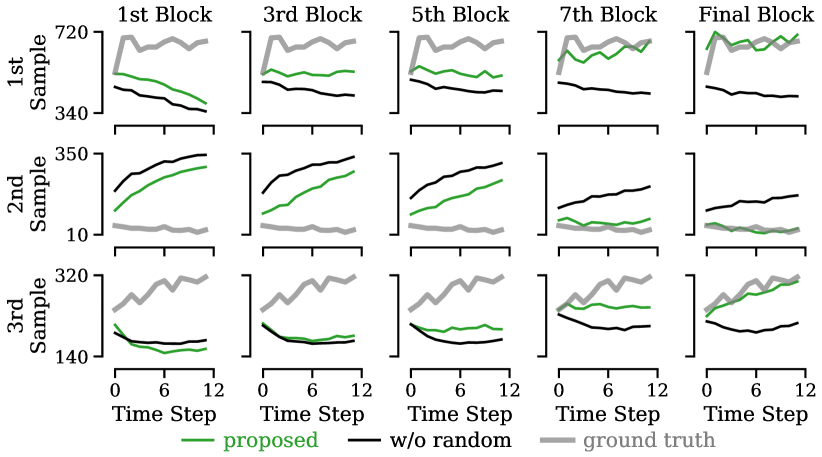
Figure 1: Each row consists of the intermediate and final outputs from a sampled node, while each column consists of the outputs from different mixer blocks within the model. The three samples are from node 238, 280, and 295 of the SD dataset (see Section 5 for details).

To illustrate that the inclusion of random projection does diversify the intermediate representation, we refer to Fig. 1, which presents three examples of the outputs from the first, third, fifth, seventh, and final (eighth) blocks of two mixer models. One of these models integrates random projection (i.e., “proposed" in Fig. 1), while the other does not. As shown, the outputs of the mixer blocks in our proposed method exhibit greater diversity (i.e., the outputs from different blocks are less similar) compared to those of alternative models that lack random projection. This diversification leads to more accurate predictions, as evidenced by the output of the final block, which closely mirrors the ground truth. Due to our application of random projection in the mixer model design, we have aptly named our proposed method RPMixer.

The key contributions of this paper include:

• We have developed a novel spatial-temporal forecasting method, RPMixer, which is both effective and efficient. We incorporate random projection layers into RPMixer to enhance the modeling diversity and capability of mixer models.

• Our ablation study highlights the importance of identity mapping for achieving the best performance of our proposed RPMixer.

• Extensive experiments validate the effectiveness of our proposed method on large-scale spatial-temporal forecasting datasets, demonstrating superior performance compared to existing solutions.

2 Related Work

In this section, we review the literature on three areas: 1) spatial-temporal forecasting methods, 2) multidimensional time series forecasting methods, and 3) random projection methods.

Spatial-temporal forecasting methods primarily use one of two spatial representations: 1) a graph-based format [24], where the spatial information is stored in a graph, and 2) a grid-based format [57], where nodes are arranged in a grid resembling an image. Given that the LargeST dataset [24] is graph-based, our review focuses on graph-based methods. These methods typically integrate graph modeling architectures, such as the graph convolutional network [17] or the graph attention network [42], with sequential modeling architectures like recurrent neural networks [14], temporal convolutional networks [30], or transformers [40]. Recent proposals include DCRNN [21], STGCN [55], ASTGCN [12], GWNET [44], AGCRN [3], STGODE [10], DSTAGNN [18], D²STGNN [35], and DGCRN [19]. We incorporate all these methods into our experiments due to their relevance to our problem. We delve into the details of these spatial-temporal forecasting methods in Appendix A.3. Note, MLPST [57], much like RPMixer, is also a mixer-type forecasting model. However, it was specifically developed for grid-based spatial-temporal forecasting problems and, therefore, is not considered in this paper.

The spatial-temporal forecasting problem, in the absence of graph input, essentially transforms into a multidimensional time series forecasting problem (see Section 3 for details). As such, we also review methods designed for multidimensional time series forecasting. Over the years, transformer-based methods [40] like LogTrans [20], Pyraformer [23], Autoformer [43], Informer [58], and Fedformer [59] have emerged. However, simple linear models outperform these transformer-based methods on multidimensional long-term time series forecasting datasets as [56] demonstrates. In contrast, mixer-based methods [37], like TSMixer [7], have demonstrated promising performance on multidimensional time series forecasting problems. Consequently, we aim to develop a mixer-based architecture for the spatial-temporal forecasting problem.

Random projection [4] is utilized in a variety of machine learning and data mining methods [4, 33, 6, 48]. However, the majority of these works [4, 6, 48] concentrate on the efficiency gains from random projection. Only [33] discusses how the diversity introduced by random projection could enhance the performance of an ensemble model, but without confirming that random projection actually introduces diversity into the model. Besides random projection, randomized methods like random shapelets/convolutions [31, 50, 54, 9] also perform exceptionally well for time series data on classification problems. Some papers also employ neural networks with partially fixed random initialized weights [15, 39, 32], but these papers neither focus on the spatial-temporal forecasting problem nor provide an analysis based on the ensemble interpretation of deep neural networks [41]. To the best of our knowledge, our paper is the first to investigate fixed randomized layers (or random projection) in the context of spatial-temporal forecasting problems.

3 Definition and Problem

We use lowercase letters (e.g., $x$), boldface lowercase letters (e.g., $\mathbf{x}$), uppercase letters (e.g., $X$), and boldface uppercase letters (e.g., $\mathbf{X}$) to denote scalars, vectors, matrices, and tensors, respectively. We begin by introducing the components of a spatial-temporal dataset. The spatial and temporal information are stored in the adjacency matrix and the time series matrix, respectively.

Definition 1.

Given that there are $n$ entities in a spatial-temporal dataset, an adjacency matrix $A\in\mathbb{R}^{n\times n}$ stores the spatial relationships among the entities, i.e., $A[i,j]$ describes the relationship between the $i$-th entity and the $j$-th entity.

Definition 2.

Given that there are $n$ entities in a spatial-temporal dataset, a time series matrix $X\in\mathbb{R}^{n\times t}$ stores the temporal information of the entities, where $t$ is the length of the time series in the dataset.

Next, we introduce the spatial-temporal forecasting problem.

Problem 1.

Given an adjacency matrix $A\in\mathbb{R}^{n\times n}$ and a historical time series matrix $X_{\text{past}}\in\mathbb{R}^{n\times t_{\text{past}}}$ for the past $t_{\text{past}}$ steps, the goal of spatial-temporal forecasting is to learn a model $F(\cdot)$ which predicts the future time series matrix $X_{\text{future}}\in\mathbb{R}^{n\times t_{\text{future}}}$ for the next $t_{\text{future}}$ steps. The problem can be formulated as: $F(X_{\text{past}},A)\rightarrow X_{\text{future}}$.

The problem formulation aligns with the multidimensional time series forecasting problem [56] if the adjacency matrix $A$ is disregarded by the model $F(\cdot)$. It is important to note that each node in a spatial-temporal dataset can be associated with multiple feature dimensions. This means that the input time series to the model $F(\cdot)$ could become a time series tensor $\mathbf{X}_{\text{past}}\in\mathbb{R}^{n\times d\times t_{\text{past}}}$, where $d$ represents the number of features of the time series and $t_{\text{past}}$ is the number of time steps in the input time series. Linear or MLP-based models can easily accommodate this additional dimensionality by reshaping the time series tensor $\mathbf{X}_{\text{past}}$ into a matrix with the shape $n\times dt_{\text{past}}$ as they utilize fully connected (linear) layers. Given the $dt_{\text{past}}$-sized vector associated with an entity, a fully connected layer is capable of utilizing information from every dimension in each past time step for the prediction.

4 Proposed Method

The proposed RPMixer adopts an all-MLP mixer architecture akin to the TSMixer [7] method, but it differs in three aspects:

1. Our design emphasizes the inclusion of identity mapping connections, achieved with a pre-activation design. The RPMixer is inspired by the ensemble interpretation of the residual connection [41], which necessitates the incorporation of identity mapping connections in the design.

2. We incorporate random projection layers in our model to increase diversity among the outputs of different mixer blocks. This is based on the ensemble interpretation, where the mixer blocks serve a similar function to the base learners in an ensemble model.

3. We process the time series in the frequency domain using complex linear layers, as time series generated from human activity are typically periodic. However, for non-periodic time series, complex layers may not be optimal. The determination of how periodic a signal should be to justify the use of complex linear layers is a topic for future research.

The overall model design is depicted in Fig. 2. Given an input historical time series matrix $X_{\text{past}}\in\mathbb{R}^{n\times t_{\text{past}}}$, the model processes it with $n_{\text{block}}$ mixer blocks, which we will introduce in the next paragraph. The output of each mixer block is also in $\mathbb{R}^{n\times t_{\text{past}}}$. The output of the last mixer block is processed by an output linear layer to project the length of the time series to the desired length (i.e., $t_{\text{future}}$). The output time series matrix is in $\mathbb{R}^{n\times t_{\text{future}}}$. We optimize the model with mean absolute error (MAE) loss.

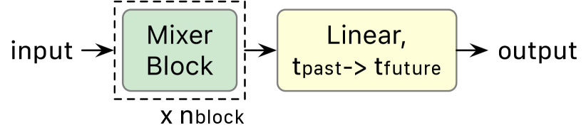
Figure 2: The RPMixer architecture.

The design of the mixer block is illustrated in Fig. 3. The highlighted forward path (in red) is used to explain the identity mapping connection in Section 4.2. The shape of the input, intermediate, and output matrices are also included in the figure. The sizes of the input and output matrices are both in $\mathbb{R}^{n\times t_{\text{past}}}$.

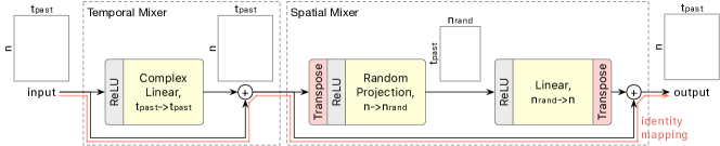
Figure 3: The detailed design of the mixer block. The red line highlighted the identity mapping connection for a mixer block.

The mixer block comprises two sub-blocks: 1) a temporal mixer block focusing on modeling the relationship between different time steps, and 2) a spatial mixer block focusing on modeling the relationship between different nodes. The temporal mixer block employs a complex linear layer after the ReLU activation function to model the time series in the frequency domain. We delve into the details of the complex linear layer in Appendix A.1.

The first and last operations of the spatial mixer block are matrix transpositions. This is done because the linear layers within the spatial mixer block are designed to model the relationship between the nodes dimension of the matrix. By transposing the matrix, we enable the linear layers to linearly combine the representations associated with each node, as opposed to time steps.

There are two types of linear layers in the spatial mixer block: 1) the random projection layer, and 2) the regular linear layer. We first use the random projection layer to project the vectors within the matrix from $\mathbb{R}^{n}$ to $\mathbb{R}^{n_{\text{rand}}}$. We regard the random projection layer as a type of linear layer because it consists of linear operations, which we implemented with a fixed, randomly initialized linear layer. We consider $n_{\text{rand}}$ a hyper-parameter of our method and provide an empirical study of this parameter in Section 5.5. The details about the random projection layer are discussed in Section 4.1. Subsequently, a regular linear layer is used to map the size of the vector within the matrix from $n_{\text{rand}}$ back to $n$. Both linear layers are preceded by a ReLU activation function.

4.1 Random Projection Layer

With the ensemble interpretation established in Section 4.2, our goal is to utilize this interpretation to further enhance the performance of our mixer model. Specifically, we aim to increase the diversity among the outputs of different base learners by incorporating random projection layers.

import torch import torch.nn as nn import torch.nn.functional as F

class RPLayer(nn.Module): def __init__(self, in_dim, out_dim, seed): super(RPLayer, self).__init__() torch.manual_seed(seed=seed) weight = torch.randn( out_dim, in_dim, requires_grad=False) self.register_buffer( ’weight’, weight, persistent=True) self.register_buffer( ’bias’, None)

def forward(self, x): return F.linear(x, self.weight, self.bias)

As demonstrated in the above pseudocode, the random projection layer is a fixed, randomly initialized linear layer that performs random projection [4] on the input. If we split the input time series matrix $X\in\mathbb{R}^{n\times t_{\text{past}}}$ into $t_{\text{past}}$ vectors of size $n$, the random projection layer computes $n_{\text{rand}}$ random combinations of the vector elements to form new vectors of size $n_{\text{rand}}$. In essence, by keeping the weights of the random projection layers fixed during training, we encourage each mixer block to concentrate on different nodes, since each random projection layer possesses its own set of randomly initialized weights.

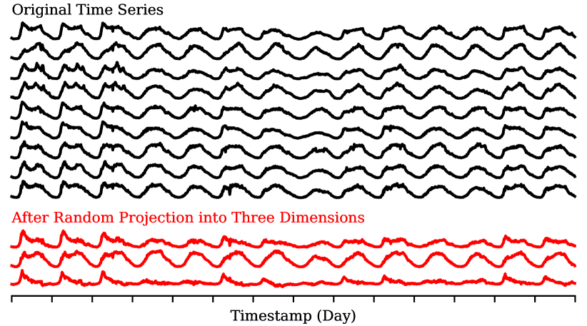
Figure 4: The time series output from a random projection layer retains the daily and weekly patterns of the original time series.

According to the Johnson-Lindenstrauss lemma [16], the relationships between the $t_{\text{past}}$ vectors are preserved after the random projection layer with high probability. This implies that the dynamics of the overall spatial-temporal data are largely retained in the data, even if it is projected to a much smaller space. To visually verify this claim, we randomly sampled nine nodes from the LargeST dataset [24] to form a nine-dimensional time series and used random projection to reduce the dimensionality to three. The visualization is shown in Fig. 4, where the daily and weekly patterns are preserved in the time series output by random projection. A similar phenomenon has been observed in [51] for the time series discord mining problem.

Another advantage of the random projection layer is its efficiency. As a dimension reduction technique [4], random projection can improve the model’s efficiency, especially when dealing with spatial-temporal data with a large number of nodes, by reducing the vector size from $n$ to a smaller $n_{\text{rand}}$. Overall, the random projection layers promote the diversity among each mixer block’s outputs while ensure efficiency.

4.2 Identity Mapping with Pre-Activation

The identity mapping connection [13] plays an important role in the ensemble interpretation [41] of the proposed RPMixer. It facilitates the creation of shorter paths, which acts like base learners within the model. We have implemented the identity mapping connection drawing inspiration from the pre-activation design proposed in [13], where the activation functions (e.g., ReLU) precede the weighted layers.

To understand why shorter paths exist within the model, we refer back to Fig. 3. We define the weighted paths for the temporal and spatial mixer sub-blocks as follows:

$$F_{\text{temp}}(X)\vcentcolon=\textsc{ComplexLinear}(\textsc{ReLU}(X))$$ (1)

$$F_{\text{sp}}(X)\vcentcolon=\textsc{Linear}(\textsc{ReLU}(\textsc{RandProject}(\textsc{ReLU}(X^{T}))))^{T}$$ (2)

Given an input $X$, the operation of the mixer block can be expressed as:

$$\textsc{Mixer}(X)=F_{\text{sp}}(F_{\text{temp}}(X)+X)+F_{\text{temp}}(X)+X$$ (3)

If we further define a function $G(\cdot)$ as:

$$G(X)\vcentcolon=F_{\text{sp}}(F_{\text{temp}}(X)+X)+F_{\text{temp}}(X)$$ (4)

The mixer block operation can be simplified to:

$$\textsc{Mixer}(X)=G(X)+X$$ (5)

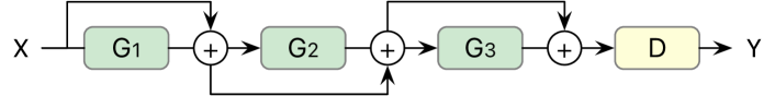
Figure 5: An example used for illustrating how the RPMixer could be interpreted as an ensemble model. In this example, there are only three mixer blocks in the model; however, the same analysis can be extended to models with more blocks.

In this equation, the first term represents the weighted path and the second term is the identity mapping connection (as shown by the red line in Fig. 3). With this simplified notation in place, let us consider the case depicted in Fig. 5, which illustrates the RPMixer with three mixer blocks. Here, we use $D(\cdot)$ to represent the output linear layer. Note, the example presented in the figure only consists of three mixer blocks, but the same analysis can be extended to models with more mixer blocks.

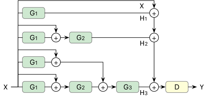
Figure 6: The unraveled view of different forward passes for the model illustrated in Fig. 5.

Following the analysis presented in [41], we can unravel the forward pass in Fig. 5 into multiple paths. The unraveled view is illustrated in Fig. 6.

If we denote the outputs of $G_{1}(\cdot)$, $G_{2}(\cdot)$, and $G_{3}(\cdot)$ as $H_{1}$, $H_{2}$, and $H_{3}$ respectively, the output $Y$ can be represented as: $Y=D(X+H_{1}+H_{2}+H_{3})$. Since $D(\cdot)$ is a linear function, the above equation can be rewritten as: $Y=D(X)+D(H_{1})+D(H_{2})+D(H_{3})$. If we further define: $Y_{0}\vcentcolon=D(X)$, $Y_{1}\vcentcolon=D(H_{1})$, $Y_{2}\vcentcolon=D(H_{2})$, and $Y_{3}\vcentcolon=D(H_{3})$, it becomes clear that the prediction $Y$ is the sum of the individual predictions from each path, i.e., $Y=Y_{0}+Y_{1}+Y_{2}+Y_{3}$. In essence, the identity mapping connections introduced by the pre-activation design facilitate an ensemble-like behavior in RPMixer.

5 Experiment

In this section, we present experiment results that demonstrate the effectiveness of our proposed method. We begin by introducing the dataset, benchmark settings, and baseline methods. Following this, we explore the benchmark results and an ablation study, which showcases the impact of each design choice. Importantly, we show how the random projection layer significantly enhances the diversity of the network’s intermediate representation, contributing substantially to the superior performance of our proposed method. Next, we conduct a sensitivity analysis on the crucial hyper-parameters. It is worth noting that our proposed method is a general approach for multivariate time series forecasting. Thus, we also perform experiments on benchmark datasets for multivariate time series forecasting and include the results in Appendix A.6. Details regarding the implementation can be found in Appendix A.4. The source code for our experiments can be downloaded from [36].

5.1 Dataset and Benchmark Setting

We conducted our experiments using the LargeST dataset [24], which consists of traffic data collected from 8,600 sensors in California from 2017 to 2021. For benchmarking purposes, we generated four sub-datasets following the procedure outlined in [24]. These sub-datasets, namely SD, GBA, GLA, and CA, include sensor data from the San Diego region, the Greater Bay Area region, the Greater Los Angeles region, and all 8,600 sensors across California, respectively. The statistics pertaining to these datasets are detailed in Appendix A.2.

In line with the experimental setup described in [24], we only utilized traffic data from 2019. Sensor readings, originally recorded at 5-minute intervals, were aggregated into 15-minute windows, yielding 96 windows per day. Each sub-dataset was chronologically divided into training, validation, and test sets at a ratio of 6:2:2. The benchmark task was to predict the next 12 steps for each sensor at each timestamp. Performance was measured using the mean absolute error (MAE), root mean squared error (RMSE), and mean absolute percentage error (MAPE).

5.2 Baseline Method

Our benchmark experiment incorporates 14 baseline methods. Besides the 11 baseline methods evaluated by Liu et al. [24], we also explore general time series forecasting baseline methods such as the one-nearest-neighbor regressor (1NN), linear model, and TSMixer [7]. It is important to note that certain baseline methods are not included for the CA dataset due to scalability issues preventing the completion of these methods’ experiments. The details about these methods are included in Appendix A.3.

Table 1: Performance comparisons. We bold the best-performing results. The performance reported in the “Average" column is computed by averaging over 12 predicted time steps. The absence of baselines on the GLA and CA datasets indicates that the models incur an out-of-memory issue. Param: the number of learnable parameters. K: $10^{3}$. M: $10^{6}$.

Data	Method	Param	Horizon 3			Horizon 6			Horizon 12			Average
			MAE	RMSE	MAPE	MAE	RMSE	MAPE	MAE	RMSE	MAPE	MAE	RMSE	MAPE
SD	HL	–	33.61	50.97	20.77%	57.80	84.92	37.73%	101.74	140.14	76.84%	60.79	87.40	41.88%
	LSTM	98K	19.17	30.75	11.85%	26.11	41.28	16.53%	38.06	59.63	25.07%	26.73	42.14	17.17%
	ASTGCN	2.2M	20.09	32.13	13.61%	25.58	40.41	17.44%	32.86	52.05	26.00%	25.10	39.91	18.05%
	DCRNN	373K	17.01	27.33	10.96%	20.80	33.03	13.72%	26.77	42.49	18.57%	20.86	33.13	13.94%
	AGCRN	761K	16.05	28.78	11.74%	18.37	32.44	13.37%	22.12	40.37	16.63%	18.43	32.97	13.51%
	STGCN	508K	18.23	30.60	13.75%	20.34	34.42	15.10%	23.56	41.70	17.08%	20.35	34.70	15.13%
	GWNET	311K	15.49	25.45	9.90%	18.17	30.16	11.98%	22.18	37.82	15.41%	18.12	30.21	12.08%
	STGODE	729K	16.76	27.26	10.95%	19.79	32.91	13.18%	23.60	41.32	16.60%	19.52	32.76	13.22%
	DSTAGNN	3.9M	17.83	28.60	11.08%	21.95	35.37	14.55%	26.83	46.39	19.62%	21.52	35.67	14.52%
	DGCRN	243K	15.24	25.46	10.09%	17.66	29.65	11.77%	21.38	36.67	14.75%	17.65	29.70	11.89%
	D2STGNN	406K	14.85	24.95	9.91%	17.28	29.05	12.17%	21.59	35.55	16.88%	17.38	28.92	12.43%
	1NN	-	21.79	35.15	13.79%	25.64	41.59	17.05%	30.77	50.59	22.38%	25.47	41.36	17.25%
	Linear	3.5K	20.58	33.30	12.98%	27.00	43.87	18.20%	32.35	53.51	22.38%	25.85	42.35	17.10%
	TSMixer	815K	17.13	27.42	11.35%	19.30	31.07	12.50%	22.03	35.70	14.26%	19.06	30.66	12.55%
	RPMixer	1.5M	15.12	24.83	9.97%	17.04	28.24	10.98%	19.60	32.96	13.12%	16.90	27.97	11.07%
GBA	HL	–	32.57	48.42	22.78%	53.79	77.08	43.01%	92.64	126.22	92.85%	56.44	79.82	48.87%
	LSTM	98K	20.41	33.47	15.60%	27.50	43.64	23.25%	38.85	60.46	37.47%	27.88	44.23	24.31%
	ASTGCN	22.3M	21.40	33.61	17.65%	26.70	40.75	24.02%	33.64	51.21	31.15%	26.15	40.25	23.29%
	DCRNN	373K	18.25	29.73	14.37%	22.25	35.04	19.82%	28.68	44.39	28.69%	22.35	35.26	20.15%
	AGCRN	777K	18.11	30.19	13.64%	20.86	34.42	16.24%	24.06	39.47	19.29%	20.55	33.91	16.06%
	STGCN	1.3M	20.62	33.81	15.84%	23.19	37.96	18.09%	26.53	43.88	21.77%	23.03	37.82	18.20%
	GWNET	344K	17.74	28.92	14.37%	20.98	33.50	17.77%	25.39	40.30	22.99%	20.78	33.32	17.76%
	STGODE	788K	18.80	30.53	15.67%	22.19	35.91	18.54%	26.27	43.07	22.71%	21.86	35.57	18.33%
	DSTAGNN	26.9M	19.87	31.54	16.85%	23.89	38.11	19.53%	28.48	44.65	24.65%	23.39	37.07	19.58%
	DGCRN	374K	18.09	29.27	15.32%	21.18	33.78	18.59%	25.73	40.88	23.67%	21.10	33.76	18.58%
	D2STGNN	446K	17.20	28.50	12.22%	20.80	33.53	15.32%	25.72	40.90	19.90%	20.71	33.44	15.23%
	1NN	-	24.84	41.30	17.70%	29.31	48.56	22.92%	35.22	58.44	31.07%	29.10	48.23	23.14%
	Linear	3.5K	21.55	34.79	17.94%	27.24	43.36	23.66%	31.50	51.56	26.18%	26.12	42.14	22.10%
	TSMixer	3.1M	17.57	29.22	14.14%	19.85	32.64	16.95%	22.27	37.60	18.63%	19.58	32.56	16.58%
	RPMixer	2.3M	17.35	28.69	13.42%	19.44	32.04	15.61%	21.65	36.20	17.42%	19.06	31.54	15.09%
GLA	HL	–	33.66	50.91	19.16%	56.88	83.54	34.85%	98.45	137.52	71.14%	59.58	86.19	38.76%
	LSTM	98K	20.09	32.41	11.82%	27.80	44.10	16.52%	39.61	61.57	25.63%	28.12	44.40	17.31%
	ASTGCN	59.1M	21.11	34.04	12.29%	28.65	44.67	17.79%	39.39	59.31	28.03%	28.44	44.13	18.62%
	DCRNN	373K	18.33	29.13	10.78%	22.70	35.55	13.74%	29.45	45.88	18.87%	22.73	35.65	13.97%
	AGCRN	792K	17.57	30.83	10.86%	20.79	36.09	13.11%	25.01	44.82	16.11%	20.61	36.23	12.99%
	STGCN	2.1M	19.87	34.01	12.58%	22.54	38.57	13.94%	26.48	45.61	16.92%	22.48	38.55	14.15%
	GWNET	374K	17.30	27.72	10.69%	21.22	33.64	13.48%	27.25	43.03	18.49%	21.23	33.68	13.72%
	STGODE	841K	18.46	30.05	11.94%	22.24	36.68	14.67%	27.14	45.38	19.12%	22.02	36.34	14.93%
	DSTAGNN	66.3M	19.35	30.55	11.33%	24.22	38.19	15.90%	30.32	48.37	23.51%	23.87	37.88	15.36%
	1NN	-	23.23	38.69	13.44%	27.75	45.92	17.07%	33.49	55.51	22.86%	27.49	45.57	17.28%
	Linear	3.5K	21.32	34.48	13.35%	27.45	43.83	17.79%	32.50	52.69	21.76%	26.40	42.56	17.16%
	TSMixer	4.6M	20.38	224.82	13.62%	22.90	229.86	15.51%	23.63	135.09	15.56%	22.12	207.68	14.87%
	RPMixer	3.2M	16.49	26.75	9.75%	18.82	30.56	11.58%	21.18	35.10	13.46%	18.46	30.13	11.34%
CA	HL	–	30.72	46.96	20.43%	51.56	76.48	37.22%	89.31	125.71	76.80%	54.10	78.97	41.61%
	LSTM	98K	19.01	31.21	13.57%	26.49	42.54	20.62%	38.41	60.42	31.03%	26.95	43.07	21.18%
	DCRNN	373K	17.52	28.18	12.55%	21.72	34.19	16.56%	28.45	44.23	23.57%	21.81	34.35	16.92%
	STGCN	4.5M	19.14	32.64	14.23%	21.65	36.94	16.09%	24.86	42.61	19.14%	21.48	36.69	16.16%
	GWNET	469K	16.93	27.53	13.14%	21.08	33.52	16.73%	27.37	42.65	22.50%	21.08	33.43	16.86%
	STGODE	1.0M	17.59	31.04	13.28%	20.92	36.65	16.23%	25.34	45.10	20.56%	20.72	36.65	16.19%
	1NN	-	21.88	36.67	15.19%	25.94	43.36	19.19%	31.29	52.52	25.65%	25.76	43.10	19.43%
	Linear	3.5K	19.82	32.39	14.73%	25.20	40.97	19.24%	29.80	49.34	23.09%	24.32	39.88	18.52%
	TSMixer	9.5M	18.40	106.28	14.30%	19.77	73.98	15.30%	22.56	87.56	17.80%	19.86	90.20	15.79%
	RPMixer	7.8M	15.90	26.08	11.69%	17.79	29.37	13.23%	19.93	33.18	15.11%	17.50	28.90	13.03%

5.3 Benchmark Result

The benchmark results are summarized in Table 1. Our discussion on the performance differences among various methods will proceed in three parts: firstly, we will discuss the 11 baselines included in the original LargeST benchmark [24]; next, we will address the three new time series forecasting baselines we added to the benchmark; finally, we will highlight the performance of our proposed RPMixer method in comparison to the baselines.

Regarding the original 11 baseline methods, HL and LSTM are typically outperformed by other methods as they do not consider inter-node relationships like the remaining nine spatial-temporal methods. Newer methods such as DGCRN and D²STGNN usually outperform other baselines. However, these two methods cannot be scaled to the two larger datasets, GLA and CA. Among older methods, AGCRN and GWNET outperform others on the SD, GBA, and GLA datasets. When considering the CA dataset, only four spatial-temporal models are applicable; GWNET, STGCN, and STGODE performance are comparable with each other.

In the case of the three new baselines (1NN, Linear, and TSMixer), both 1NN and Linear perform poorly for the same reason as the HL and LSTM baselines: these methods do not model the relationship between the nodes. When comparing TSMixer with the original 11 baseline methods, it is comparable with the best method on the two smaller datasets (SD and GBA). However, it performs noticeably worse in terms of RMSE on the two larger datasets (GLA and CA). A possible reason is that TSMixer is overfitting to MAE, which also serves as the loss function when training the model. Despite TSMixer’s high parameter count, it can still be applied to the largest dataset (CA) because the memory scales linearly with respect to the number of nodes, unlike the more expensive graph-based baselines (ASTGCN, AGCRN, DSTAGNN, DGCRN, and D²STGNN).

For smaller datasets such as SD and GBA, RPMixer surpasses the performance of baseline methods in the later time steps of the predictions. When it comes to larger datasets like GLA and CA, RPMixer outperforms all baseline methods across every performance measure and time horizon. Even though the proposed method has a high number of parameters similar to TSMixer, it is not overfitting to the loss function and performs exceptionally well across the board. The memory complexity of RPMixer scales linearly with respect to the number of nodes, enabling it to be applied to the largest dataset (CA).

5.4 Ablation Study

We conducted an ablation study on the three most crucial design decisions associated with our proposed RPMixer method. The three decisions were: 1) implementing the identity mapping connection with pre-activation, 2) introducing random projection layers, and 3) processing the time series in the frequency domain. The results of the ablation study are presented in Fig. 7.

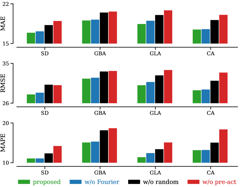
Figure 7: The ablation study result measured using average MAE, RMSE, and MAPE. Removing each component resulted in a degradation of the performance.

The pre-activation design emerged as the most consequential design decision. Upon its replacement with a post-activation design, we effectively removed the most important element of the original design, leading to a significant performance decrease. This decline is likely due to the elimination of identity mapping connections from the network. These connections are vital for the ensemble interpretation of the residual connection. Without them, the inclusion of a random projection layer no longer makes sense, as it weakens the ensemble-like-like behavior of the residual blocks (i.e., the mixer blocks in RPMixer), which was the motivation behind the design of the random projection layer.

The random projection layer design was the second most important decision in terms of performance difference. We disabled the random projection layer by converting it into a regular linear layer with trainable weights. This layer helps each mixer block in focusing on different aspects of the inter-node relationship, so its importance is not surprising. To verify our claim that the random projection layer promotes diversity, we constructed a correlation-error diagram comparing the proposed method with the variant without random projection layer. This diagram serves a similar purpose to the kappa-error diagram [27] used for analyzing base learners in an ensemble model. Before discussing the diagram, let us first introduce what a correlation-error diagram is.

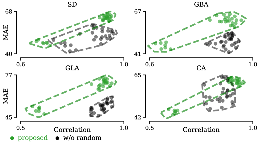
Figure 8: The correlation-error diagram illustrates the interplay of diversity and error (MAE) across individual blocks in the model.

A correlation-error diagram is a visualization tool akin to the kappa-error diagram [27], used for analyzing the trade-off between performance and diversity in ensemble models. Each dot in the diagram represents a pair of base learners, with the $y$-axis showing the average performance of the pair’s outputs and the $x$-axis indicating the degree of agreement between them. Specifically, we use the Pearson correlation coefficient to measure agreement between the outputs of a pair of mixer blocks (i.e., the base learners). We use MAE, RMSE, and MAPE as performance measures. The figure created using MAE and Pearson correlation coefficient is shown in Fig. 8. Figures using other performance measures are included in Appendix A.5. We observe that the dots associated with the proposed method with a random projection layer have a wider distribution (larger range in $y$-axis) compared to the variant without the random projection layer. This confirms that our random projection layer effectively increases the diversity of the intermediate representation.

The decision to process the time series in the frequency domain had the least impact on performance. The performance improvement is minor compared to the other two design choices. One possible reason is that the Fourier transformation is a linear transformation, so the majority of its benefits could be learned by the model during training. We also analyze the effect of different design choices at various time horizons and the findings are reported in Appendix A.5.

5.5 Parameter Sensitivity Analysis

In our parameter sensitivity analysis, we focus on two hyper-parameters: the number of mixer blocks and the number of neurons in the random projection layer. We report performance on both the validation and test sets to demonstrate the generalizability of our findings across different data partitions. Fig. 9(a) illustrates the parameter sensitivity analysis for the number of mixer blocks.

(a) Setting the number of block to eight generally yields better results. This observation holds true for both validation and test data.

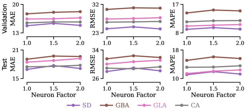
(b) The number is set by $m_{neuron}\sqrt{n}$, where $n$ is the number of nodes in the graph and $m_{neuron}$ is a factor. Setting this factor to one often has the best performance. This observation holds true for both validation and test data.

Figure 9: The parameter sensitivity analysis for the number of block and number of neurons parameter measured using average MAE, RMSE, and MAPE.

Setting the number of blocks to eight generally yields the best performance on both the validation and test data. Reducing the number of blocks to two significantly diminishes performance, indicating the necessity of multiple blocks to achieve ensemble-like behavior. Increasing the number of blocks to 16 results in minor performance improvement on some datasets. However, as it doubles the model size, the minor gain in performance may not justify the increased computational cost. Similar trends are observed on both the validation and test data, suggesting that we can use the validation set to tune this hyper-parameter.

For the number of neurons in the random projection layer, we set it as a function with respect to the number of nodes in the spatial-temporal data, as more neurons may be required for datasets with larger number of nodes. If the graph has $n$ nodes, we set the number of neurons in the random projection layer as $m_{neuron}\sqrt{n}$, where $m_{neuron}$ is the hyper-parameter controlling the number of neurons in the layer. This design allows the model to automatically use more neurons for datasets with more number of nodes, even if the hyper-parameter $m_{neuron}$ is set to the same value for all datasets. Fig. 9(b) displays the results of the parameter sensitivity analysis for the hyper-parameter $m_{neuron}$.

We evaluated the model under three different settings of $m_{neuron}$: $\{1.0,1.5,2.0\}$. Our observation indicates that setting the hyper-parameter to 1.0 generally leads to good performance, although for some datasets, a setting of 2.0 may yield better results. However, the performance difference is minimal and may not justify the additional computational cost associated with the 2.0 setting. Additionally, the trends on the validation data closely mirror those on the testing data, justifying the use of validation data for setting the hyper-parameter.

6 Conclusion

In this paper, we proposed RPMixer, an all-MLP mixer model that incorporates random projection layers. These layers enhance the diversity among the outputs of each mixer block, thereby improving the overall performance of the model. Our experiments demonstrated that the random projection layers not only improve the diversity of the intermediate representation but also boost the model’s overall performance on large-scale spatial-temporal benchmark datasets in the literature [24]. This work contributes a new approach to spatial-temporal forecasting, potentially providing more accurate and reliable predictions for real-world applications such as traffic flow prediction. In future work, we plan to investigate the potential of applying time series foundation models [47] for tackling spatial-temporal forecasting problems.

Appendix A Supplementary

In this section, we provide supplementary materials for the paper. These materials encompass additional details and results that were excluded from the primary text due to space constraints.

A.1 Complex Linear Layer

As depicted in Fig. 10, the time series in the large spatial-temporal forecasting benchmark dataset exhibits periodicity.

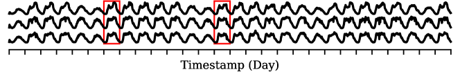
Figure 10: The time series for three randomly selected nodes from the LargeST dataset spans a period of four weeks.

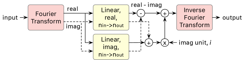
Figure 11: The complex linear layer.

To leverage this periodicity, we opt to process the time series in the frequency domain using a complex linear layer [38]. The computational graph for the complex linear layer is illustrated in Fig. 11. Initially, the input data is converted to the frequency domain using the Fast Fourier Transform (FFT) method. Subsequently, the real and imaginary parts are processed by two distinct linear layers, one containing the real part of the model weights and the other containing the imaginary part. The outputs from these two linear layers are then combined, and finally an inverse FFT layer is used to convert back to the time domain.

The design rationale stems from the fact that, unlike regular linear layers, the weights for the complex linear layer are complex numbers. Consider a simplified scenario where we aim to multiply input data $x$ with a complex weight matrix $W_{\text{real}}+{i\mkern 1.0mu}W_{\text{imag}}$. As depicted in Fig. 11, the input data $x$ is first converted to the frequency domain as $x_{\text{real}}+{i\mkern 1.0mu}x_{\text{imag}}$ using the FFT method. Next, we multiply $x_{\text{real}}+{i\mkern 1.0mu}x_{\text{imag}}$ with $W_{\text{real}}+{i\mkern 1.0mu}W_{\text{imag}}$. Simple algebraic manipulation reveals that the result of this multiplication is

$$(W_{\text{real}}x_{\text{real}}-W_{\text{imag}}x_{\text{imag}})+{i\mkern 1.0mu}(W_{\text{real}}x_{\text{imag}}+W_{\text{imag}}x_{\text{real}})$$ (6)

This operation is captured in the design illustrated in Fig. 11.

A.2 Dataset Statistics

The statistics for the SD, GBA, GLA, and CA dataset are summarized in Table 2.

Table 2: Dataset statistics.

Data	# of nodes	# of time steps	time range
SD	716	35,040	[1/1/2019, 1/1/2020)
GBA	2,352	35,040	[1/1/2019, 1/1/2020)
GLA	3,834	35,040	[1/1/2019, 1/1/2020)
CA	8,600	35,040	[1/1/2019, 1/1/2020)

A.3 Baseline Method

The details about the 14 baseline methods are provided below:

• HL: The prediction for all future time steps is generated by using the last value from the historical data.

• LSTM [14]: The Long Short-Term Memory (LSTM), a variant of the recurrent neural network architecture, is specifically designed to process sequential data, making it a general method for time series forecasting. When deploying this architecture on the LargeST dataset, the same model weights are utilized across the time series of different nodes.

• ASTGCN [12]: The Attention-based Spatial-Temporal Graph Convolutional Network (ASTGCN) model employs a spatial-temporal attention mechanism to capture spatial-temporal correlations. It also uses graph convolutions and conventional convolutions to extract spatial and temporal patterns, respectively.

• DCRNN [21]: The Diffusion Convolutional Recurrent Neural Network (DCRNN) incorporates diffusion convolution, the sequence-to-sequence architecture, and the scheduled sampling technique to capture spatial-temporal patterns.

• AGCRN [3]: The Adaptive Graph Convolutional Recurrent Network (AGCRN) extends the design of recurrent networks with a node adaptive parameter learning module, enabling the capture of node-specific patterns. Additionally, it includes a data adaptive graph generation module to infer the interdependencies among different nodes.

• STGCN [55]: The Spatial-Temporal Graph Convolutional Networks (STGCN) employs both graph and temporal convolutions to model the spatial-temporal correlations within the data.

• GWNET [44]: The Graph WaveNet (GWNET) is another network that relies on convolution operations. Specifically, it employs a gated temporal convolution module and a graph convolution layer to model the spatial-temporal correlation.

• STGODE [10]: The Spatial-Temporal Graph Ordinary Differential Equation Networks (STGODE) models spatial-temporal dynamics using tensor-based ordinary differential equations. The model design also incorporates a semantical adjacency matrix and temporal dilated convolution modules.

• DSTAGNN [18]: The Dynamic Spatial-Temporal Aware Graph Neural Network (DSTAGNN) is a method that does not use a predefined static adjacency matrix. Instead, it learns the dynamic spatial associations among nodes and utilizes a spatial-temporal attention module based on multi-order Chebyshev polynomials to capture these associations. To model the temporal associations, it employs gated convolution modules.

• DGCRN [19]: The Dynamic Graph Convolutional Recurrent Network (DGCRN) model combines graph convolution networks with recurrent networks. In this model, a dynamic adjacency matrix is progressively generated by a hyper-network in synchronization with the recurrent steps. This dynamic adjacency matrix, in conjunction with the predefined static adjacency matrix, is utilized to generate predictions.

• D²STGNN [35]: The Decoupled Dynamic Spatial-Temporal Graph Neural Network (D²STGNN) decouples the diffusion and inherent information in a data-driven manner using an estimation gate and a residual decomposition mechanism. Additionally, it employs a dynamic graph learning module that learns the dynamic characteristics of the spatial-temporal graph.

• 1NN: The 1-Nearest-Neighbor (1NN) method serves as a simple baseline for a range of time series problems [2, 8]. We have implemented this baseline by leveraging the matrix profile for its efficiency [53, 60]. Notably, the version of the 1NN method benchmarked in this study is the most basic form, where each node is treated as independent from the others. While more advanced techniques from the literature, such as those presented in [49, 28, 52], could potentially enhance the method, we plan to explore these techniques in our future work.

• Linear: Having proven its effectiveness in general time series forecasting [56], the linear model has been incorporated into our benchmark experiments. Similar to LSTM, the same model weights are used across the time series of various nodes.

• TSMixer [7]: The Time Series Mixer (TSMixer) is a stacked Multi-Layer Perceptron (MLP) that efficiently extracts information by utilizing mixing operations across both the time and feature dimensions (i.e., nodes for spatial-temporal data). These mixing operations are capable of capturing the relationships between different time steps and nodes.

A.4 Implementation Detail

The experiments were carried out using Python 3.10.11 on a Linux server equipped with an AMD EPYC 7713 64-Core Processor and NVIDIA Tesla A100 GPU. Our implementation leverages PyTorch 2.0.1 to realize the proposed RPMixer, TSMixer, and the Linear model. All three models are trained using the AdamW optimizer [26] with default hyper-parameter settings. The MAE loss function was used, following [24]. In the case of the proposed method, we configure the number of mixer blocks to eight and set the random projection dimension to $\sqrt{n}$, where $n$ is the number of nodes in the graph. For TSMixer, the number of mixer blocks is also set to eight, and the number of hidden dimensions is fixed at 64, in accordance with the parameterization used by the original author in the Traffic prediction dataset experiment [7]. The 1NN method is implemented using pyscamp 0.4.0 [60]. Further details on our implementation can be found in the released source code [36].

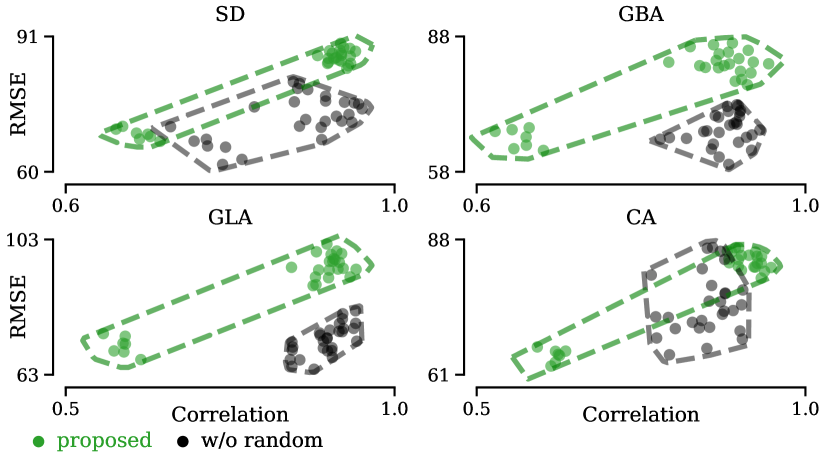
(a) RMSE

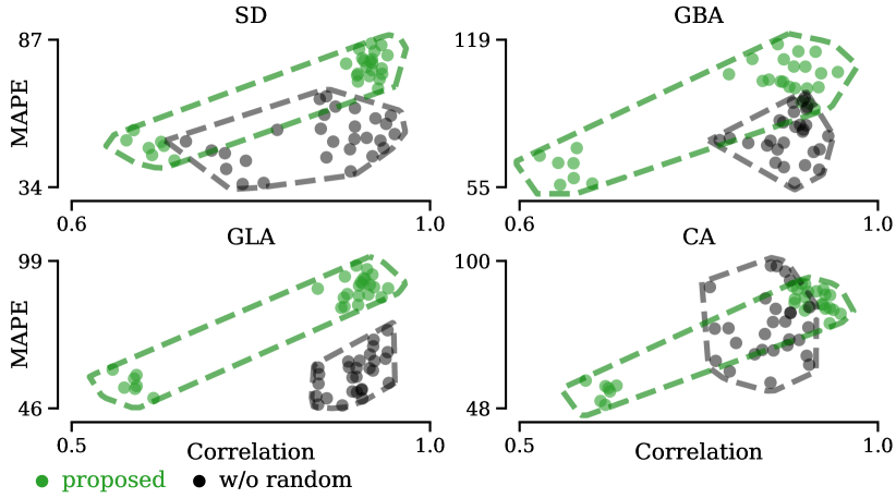
(b) MAPE

Figure 12: The correlation-error diagram illustrates the interplay of diversity and error (RMSE and MAPE) across individual blocks in the model.

A.5 Ablation Study

We have produced correlation-error diagrams employing all three measurements (MAE, RMSE, and MAPE). In Section 5.4, we showcase the correlation-error diagram with MAE in Fig. 8. This section introduces the remaining two correlation-error diagrams, namely, the correlation-error diagram with RMSE in Fig. 12(a), and the correlation-error diagram with MAPE in Fig. 12(b). The conclusions remain consistent. The random projection layer aids the proposed method in achieving greater diversity.

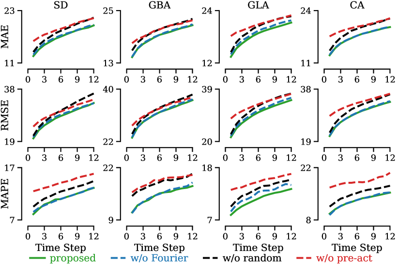
Figure 13: The ablation study result measured using per-step MAE, RMSE, and MAPE. The random projection layer benefits the prediction for later time steps more compared to earlier time steps.

To understand the effect of different design choices at various time horizons, we visualized the performance of different variants of the proposed model over the prediction time steps in Fig. 13. For the pre-activation and frequency domain choices, the positive effect is evenly distributed across different time steps. For the random projection layer, the benefits lean more towards longer-term predictions. A possible explanation is that the variance for longer-term prediction is typically higher. Since the random projection layer helps different mixer blocks focus on different dimensions of the multivariate time series, it aids the model in better capturing the later, harder-to-predict time steps.

A.6 Long-Term Time Series Forecasting

The effectiveness of the proposed method in spatial-temporal forecasting tasks has been demonstrated. However, as a general time series forecasting method, we sought to assess its performance against other forecasting methods. To this end, we evaluated our method on seven multivariate long-term time series forecasting datasets (i.e., ETTh1, ETTh2, ETTm1, ETTm2, Weather, Electricity, and Traffic), and compared it with two state-of-the-art methods, TSMixer [7] and PatchTST [29], which have shown superior performance over alternatives such as Autoformer [43], Informer [58], TFT [22], FEDformer [59], and linear models [56].

The experimental setup followed the guidelines outlined in [29, 7]. We evaluated the models under long-term time series forecasting settings, with prediction lengths of 96, 192, 336, and 720. The evaluation metrics employed were mean square error (MSE) and mean absolute error (MAE). The dataset was divided into training, validation, and testing subsets, as suggested in [29, 7, 56]. The input length was set to 512 as per [7], and other hyper-parameters were determined based on the validation set results. The settings for the hyper-parameters are provided with the source code, which can be downloaded from [36]. We employed the AdamW optimizer [26] with the objective of minimizing the mean square error. The results are presented in Table 3.

Table 3: Performance comparisons. We bold the best-performing results.

Data	Method	Horizon 96		Horizon 192		Horizon 336		Horizon 720
		MSE	MAE	MSE	MAE	MSE	MAE	MSE	MAE
ETTh1	PatchTST	0.370	0.400	0.413	0.429	0.422	0.440	0.447	0.468
	TSMixer	0.361	0.392	0.404	0.418	0.420	0.431	0.463	0.472
	RPMixer	0.444	0.444	0.488	0.475	0.521	0.498	0.625	0.574
ETTh2	PatchTST	0.274	0.337	0.341	0.382	0.329	0.384	0.379	0.422
	TSMixer	0.274	0.341	0.339	0.385	0.361	0.406	0.445	0.470
	RPMixer	0.173	0.284	0.210	0.317	0.246	0.346	0.340	0.410
ETTm1	PatchTST	0.293	0.346	0.333	0.370	0.369	0.392	0.416	0.420
	TSMixer	0.285	0.339	0.327	0.365	0.356	0.382	0.419	0.414
	RPMixer	0.358	0.385	0.397	0.406	0.439	0.433	0.503	0.475
ETTm2	PatchTST	0.166	0.256	0.223	0.296	0.274	0.329	0.362	0.385
	TSMixer	0.163	0.252	0.216	0.290	0.268	0.324	0.420	0.422
	RPMixer	0.111	0.224	0.139	0.252	0.168	0.276	0.212	0.311
Weather	PatchTST	0.149	0.198	0.194	0.241	0.245	0.282	0.314	0.334
	TSMixer	0.145	0.198	0.191	0.242	0.242	0.280	0.320	0.336
	RPMixer	0.149	0.206	0.198	0.250	0.258	0.295	0.343	0.353
Electricity	PatchTST	0.129	0.222	0.147	0.240	0.163	0.259	0.197	0.290
	TSMixer	0.131	0.229	0.151	0.246	0.161	0.261	0.197	0.293
	RPMixer	0.130	0.229	0.149	0.247	0.166	0.264	0.201	0.302
Traffic	PatchTST	0.360	0.249	0.379	0.256	0.392	0.264	0.432	0.286
	TSMixer	0.376	0.264	0.397	0.277	0.413	0.290	0.444	0.306
	RPMixer	0.394	0.277	0.406	0.282	0.415	0.286	0.451	0.307

The results suggest that our proposed method performs comparably to both TSMixer and PatchTST, as confirmed by a $t$-test with $\alpha=0.05$. This implies that the proposed method also achieves state-of-the-art performance on the long-term time series forecasting tasks. Chen et al. [7] noted that the cross-variate information might not be as significant in these seven datasets. Therefore, the fact that our proposed method achieves state-of-the-art performance indicates that its components for capturing cross-variate information do not degrade performance, even when the cross-variate information is not relevant for the task. This suggests that our method is robust against irrelevant cross-variate information.

References

- [1]
- Bagnall et al. [2017] Anthony Bagnall, Jason Lines, Aaron Bostrom, James Large, and Eamonn Keogh. 2017. The great time series classification bake off: a review and experimental evaluation of recent algorithmic advances. Data mining and knowledge discovery 31 (2017), 606–660.
- Bai et al. [2020] Lei Bai, Lina Yao, Can Li, Xianzhi Wang, and Can Wang. 2020. Adaptive graph convolutional recurrent network for traffic forecasting. Advances in neural information processing systems 33 (2020), 17804–17815.
- Bingham and Mannila [2001] Ella Bingham and Heikki Mannila. 2001. Random projection in dimensionality reduction: applications to image and text data. In Proceedings of the seventh ACM SIGKDD international conference on Knowledge discovery and data mining. 245–250.
- Cai et al. [2023] Zekun Cai, Renhe Jiang, Xinyu Yang, Zhaonan Wang, Diansheng Guo, Hiroki Kobayashi, Xuan Song, and Ryosuke Shibasaki. 2023. MemDA: Forecasting Urban Time Series with Memory-based Drift Adaptation. arXiv preprint arXiv:2309.14216 (2023).
- Cannings and Samworth [2017] Timothy I Cannings and Richard J Samworth. 2017. Random-projection ensemble classification. Journal of the Royal Statistical Society Series B: Statistical Methodology 79, 4 (2017), 959–1035.
- Chen et al. [2023] Si-An Chen, Chun-Liang Li, Nate Yoder, Sercan O Arik, and Tomas Pfister. 2023. Tsmixer: An all-mlp architecture for time series forecasting. arXiv preprint arXiv:2303.06053 (2023).
- Dau et al. [2019] Hoang Anh Dau, Anthony Bagnall, Kaveh Kamgar, Chin-Chia Michael Yeh, Yan Zhu, Shaghayegh Gharghabi, Chotirat Ann Ratanamahatana, and Eamonn Keogh. 2019. The UCR time series archive. IEEE/CAA Journal of Automatica Sinica 6, 6 (2019), 1293–1305.
- Dempster et al. [2020] Angus Dempster, François Petitjean, and Geoffrey I Webb. 2020. ROCKET: exceptionally fast and accurate time series classification using random convolutional kernels. Data Mining and Knowledge Discovery 34, 5 (2020), 1454–1495.
- Fang et al. [2021] Zheng Fang, Qingqing Long, Guojie Song, and Kunqing Xie. 2021. Spatial-temporal graph ode networks for traffic flow forecasting. In Proceedings of the 27th ACM SIGKDD conference on knowledge discovery & data mining. 364–373.
- Geng et al. [2019] Xu Geng, Yaguang Li, Leye Wang, Lingyu Zhang, Qiang Yang, Jieping Ye, and Yan Liu. 2019. Spatiotemporal multi-graph convolution network for ride-hailing demand forecasting. In Proceedings of the AAAI conference on artificial intelligence, Vol. 33. 3656–3663.
- Guo et al. [2019] Shengnan Guo, Youfang Lin, Ning Feng, Chao Song, and Huaiyu Wan. 2019. Attention based spatial-temporal graph convolutional networks for traffic flow forecasting. In Proceedings of the AAAI conference on artificial intelligence, Vol. 33. 922–929.
- He et al. [2016] Kaiming He, Xiangyu Zhang, Shaoqing Ren, and Jian Sun. 2016. Identity mappings in deep residual networks. In Computer Vision–ECCV 2016: 14th European Conference, Amsterdam, The Netherlands, October 11–14, 2016, Proceedings, Part IV 14. Springer, 630–645.
- Hochreiter and Schmidhuber [1997] Sepp Hochreiter and Jürgen Schmidhuber. 1997. Long short-term memory. Neural computation 9, 8 (1997), 1735–1780.
- Huang et al. [2015] Gao Huang, Guang-Bin Huang, Shiji Song, and Keyou You. 2015. Trends in extreme learning machines: A review. Neural Networks 61 (2015), 32–48.
- Johnson [1984] William B Johnson. 1984. Extensions of Lipshitz mapping into Hilbert space. In Conference modern analysis and probability, 1984. 189–206.
- Kipf and Welling [2016] Thomas N Kipf and Max Welling. 2016. Semi-supervised classification with graph convolutional networks. arXiv preprint arXiv:1609.02907 (2016).
- Lan et al. [2022] Shiyong Lan, Yitong Ma, Weikang Huang, Wenwu Wang, Hongyu Yang, and Pyang Li. 2022. Dstagnn: Dynamic spatial-temporal aware graph neural network for traffic flow forecasting. In International conference on machine learning. PMLR, 11906–11917.
- Li et al. [2023] Fuxian Li, Jie Feng, Huan Yan, Guangyin Jin, Fan Yang, Funing Sun, Depeng Jin, and Yong Li. 2023. Dynamic graph convolutional recurrent network for traffic prediction: Benchmark and solution. ACM Transactions on Knowledge Discovery from Data 17, 1 (2023), 1–21.
- Li et al. [2019] Shiyang Li, Xiaoyong Jin, Yao Xuan, Xiyou Zhou, Wenhu Chen, Yu-Xiang Wang, and Xifeng Yan. 2019. Enhancing the locality and breaking the memory bottleneck of transformer on time series forecasting. Advances in neural information processing systems 32 (2019).
- Li et al. [2017] Yaguang Li, Rose Yu, Cyrus Shahabi, and Yan Liu. 2017. Diffusion convolutional recurrent neural network: Data-driven traffic forecasting. arXiv preprint arXiv:1707.01926 (2017).
- Lim et al. [2021] Bryan Lim, Sercan Ö Arık, Nicolas Loeff, and Tomas Pfister. 2021. Temporal fusion transformers for interpretable multi-horizon time series forecasting. International Journal of Forecasting 37, 4 (2021), 1748–1764.
- Liu et al. [2021] Shizhan Liu, Hang Yu, Cong Liao, Jianguo Li, Weiyao Lin, Alex X Liu, and Schahram Dustdar. 2021. Pyraformer: Low-complexity pyramidal attention for long-range time series modeling and forecasting. In International conference on learning representations.
- Liu et al. [2023] Xu Liu, Yutong Xia, Yuxuan Liang, Junfeng Hu, Yiwei Wang, Lei Bai, Chao Huang, Zhenguang Liu, Bryan Hooi, and Roger Zimmermann. 2023. LargeST: A Benchmark Dataset for Large-Scale Traffic Forecasting. arXiv preprint arXiv:2306.08259 (2023).
- Liu et al. [2020] Ziyu Liu, Hongwen Zhang, Zhenghao Chen, Zhiyong Wang, and Wanli Ouyang. 2020. Disentangling and unifying graph convolutions for skeleton-based action recognition. In Proceedings of the IEEE/CVF conference on computer vision and pattern recognition. 143–152.
- Loshchilov and Hutter [2017] Ilya Loshchilov and Frank Hutter. 2017. Decoupled weight decay regularization. arXiv preprint arXiv:1711.05101 (2017).
- Margineantu and Dietterich [1997] Dragos D Margineantu and Thomas G Dietterich. 1997. Pruning Adaptive Boosting. In Proceedings of the Fourteenth International Conference on Machine Learning. 211–218.
- Martínez et al. [2019] Francisco Martínez, María Pilar Frías, María Dolores Pérez, and Antonio Jesús Rivera. 2019. A methodology for applying k-nearest neighbor to time series forecasting. Artificial Intelligence Review 52, 3 (2019), 2019–2037.
- Nie et al. [2022] Yuqi Nie, Nam H Nguyen, Phanwadee Sinthong, and Jayant Kalagnanam. 2022. A time series is worth 64 words: Long-term forecasting with transformers. arXiv preprint arXiv:2211.14730 (2022).
- Oord et al. [2016] Aaron van den Oord, Sander Dieleman, Heiga Zen, Karen Simonyan, Oriol Vinyals, Alex Graves, Nal Kalchbrenner, Andrew Senior, and Koray Kavukcuoglu. 2016. Wavenet: A generative model for raw audio. arXiv preprint arXiv:1609.03499 (2016).
- Renard et al. [2016] Xavier Renard, Maria Rifqi, Gabriel Fricout, and Marcin Detyniecki. 2016. EAST representation: fast discovery of discriminant temporal patterns from time series. In ECML/PKDD Workshop on Advanced Analytics and Learning on Temporal Data.
- Rosenfeld and Tsotsos [2019] Amir Rosenfeld and John K Tsotsos. 2019. Intriguing properties of randomly weighted networks: Generalizing while learning next to nothing. In 2019 16th conference on computer and robot vision (CRV). IEEE, 9–16.
- Schclar and Rokach [2009] Alon Schclar and Lior Rokach. 2009. Random projection ensemble classifiers. In Enterprise Information Systems: 11th International Conference, ICEIS 2009, Milan, Italy, May 6-10, 2009. Proceedings 11. Springer, 309–316.
- Shang et al. [2021] Chao Shang, Jie Chen, and Jinbo Bi. 2021. Discrete graph structure learning for forecasting multiple time series. arXiv preprint arXiv:2101.06861 (2021).
- Shao et al. [2022] Zezhi Shao, Zhao Zhang, Wei Wei, Fei Wang, Yongjun Xu, Xin Cao, and Christian S Jensen. 2022. Decoupled dynamic spatial-temporal graph neural network for traffic forecasting. arXiv preprint arXiv:2206.09112 (2022).
- The Author(2023) [s] The Author(s). 2023. Project Website. https://sites.google.com/view/rpmixer.
- Tolstikhin et al. [2021] Ilya O Tolstikhin, Neil Houlsby, Alexander Kolesnikov, Lucas Beyer, Xiaohua Zhai, Thomas Unterthiner, Jessica Yung, Andreas Steiner, Daniel Keysers, Jakob Uszkoreit, et al. 2021. Mlp-mixer: An all-mlp architecture for vision. Advances in neural information processing systems 34 (2021), 24261–24272.
- Trabelsi et al. [2018] Chiheb Trabelsi, Olexa Bilaniuk, Ying Zhang, Dmitriy Serdyuk, Sandeep Subramanian, João Felipe Santos, Soroush Mehri, Negar Rostamzadeh, Yoshua Bengio, and Christopher J Pal. 2018. Deep Complex Networks. arXiv:1705.09792 [cs.NE]
- Ulyanov et al. [2018] Dmitry Ulyanov, Andrea Vedaldi, and Victor Lempitsky. 2018. Deep image prior. In Proceedings of the IEEE conference on computer vision and pattern recognition. 9446–9454.
- Vaswani et al. [2017] Ashish Vaswani, Noam Shazeer, Niki Parmar, Jakob Uszkoreit, Llion Jones, Aidan N Gomez, Łukasz Kaiser, and Illia Polosukhin. 2017. Attention is all you need. Advances in neural information processing systems 30 (2017).
- Veit et al. [2016] Andreas Veit, Michael J Wilber, and Serge Belongie. 2016. Residual networks behave like ensembles of relatively shallow networks. Advances in neural information processing systems 29 (2016).
- Veličković et al. [2017] Petar Veličković, Guillem Cucurull, Arantxa Casanova, Adriana Romero, Pietro Lio, and Yoshua Bengio. 2017. Graph attention networks. arXiv preprint arXiv:1710.10903 (2017).
- Wu et al. [2021] Haixu Wu, Jiehui Xu, Jianmin Wang, and Mingsheng Long. 2021. Autoformer: Decomposition transformers with auto-correlation for long-term series forecasting. Advances in Neural Information Processing Systems 34 (2021), 22419–22430.
- Wu et al. [2019] Zonghan Wu, Shirui Pan, Guodong Long, Jing Jiang, and Chengqi Zhang. 2019. Graph wavenet for deep spatial-temporal graph modeling. arXiv preprint arXiv:1906.00121 (2019).
- Yan et al. [2018] Sijie Yan, Yuanjun Xiong, and Dahua Lin. 2018. Spatial temporal graph convolutional networks for skeleton-based action recognition. In Proceedings of the AAAI conference on artificial intelligence, Vol. 32.
- Yao et al. [2018] Huaxiu Yao, Fei Wu, Jintao Ke, Xianfeng Tang, Yitian Jia, Siyu Lu, Pinghua Gong, Jieping Ye, and Zhenhui Li. 2018. Deep multi-view spatial-temporal network for taxi demand prediction. In Proceedings of the AAAI conference on artificial intelligence, Vol. 32.
- Yeh et al. [2023a] Chin-Chia Michael Yeh, Xin Dai, Huiyuan Chen, Yan Zheng, Yujie Fan, Audrey Der, Vivian Lai, Zhongfang Zhuang, Junpeng Wang, Liang Wang, et al. 2023a. Toward a foundation model for time series data. In Proceedings of the 32nd ACM International Conference on Information and Knowledge Management. 4400–4404.
- Yeh et al. [2022a] Chin-Chia Michael Yeh, Mengting Gu, Yan Zheng, Huiyuan Chen, Javid Ebrahimi, Zhongfang Zhuang, Junpeng Wang, Liang Wang, and Wei Zhang. 2022a. Embedding Compression with Hashing for Efficient Representation Learning in Large-Scale Graph. In Proceedings of the 28th ACM SIGKDD Conference on Knowledge Discovery and Data Mining. 4391–4401.
- Yeh et al. [2017] Chin-Chia Michael Yeh, Nickolas Kavantzas, and Eamonn Keogh. 2017. Matrix profile VI: Meaningful multidimensional motif discovery. In 2017 IEEE international conference on data mining (ICDM). IEEE, 565–574.
- Yeh and Keogh [2016] Chin-Chia Michael Yeh and Eamonn Keogh. 2016. The First Place Solution to the AALTD’16 Challenge. https://github.com/mcyeh/aaltd16_fusion.
- Yeh et al. [2023b] Chin-Chia Michael Yeh, Yan Zheng, Menghai Pan, Huiyuan Chen, Zhongfang Zhuang, Junpeng Wang, Liang Wang, Wei Zhang, Jeff M Phillips, and Eamonn Keogh. 2023b. Sketching multidimensional time series for fast discord mining. arXiv preprint arXiv:2311.03393 (2023).
- Yeh et al. [2022b] Chin-Chia Michael Yeh, Yan Zheng, Junpeng Wang, Huiyuan Chen, Zhongfang Zhuang, Wei Zhang, and Eamonn Keogh. 2022b. Error-bounded approximate time series joins using compact dictionary representations of time series. In Proceedings of the 2022 SIAM International Conference on Data Mining (SDM). SIAM, 181–189.
- Yeh et al. [2016] Chin-Chia Michael Yeh, Yan Zhu, Liudmila Ulanova, Nurjahan Begum, Yifei Ding, Hoang Anh Dau, Diego Furtado Silva, Abdullah Mueen, and Eamonn Keogh. 2016. Matrix profile I: all pairs similarity joins for time series: a unifying view that includes motifs, discords and shapelets. In 2016 IEEE 16th international conference on data mining (ICDM). Ieee, 1317–1322.
- Yeh [2018] Michael Chin-Chia Yeh. 2018. Towards a near universal time series data mining tool: Introducing the matrix profile. University of California, Riverside.
- Yu et al. [2017] Bing Yu, Haoteng Yin, and Zhanxing Zhu. 2017. Spatio-temporal graph convolutional networks: A deep learning framework for traffic forecasting. arXiv preprint arXiv:1709.04875 (2017).
- Zeng et al. [2023] Ailing Zeng, Muxi Chen, Lei Zhang, and Qiang Xu. 2023. Are transformers effective for time series forecasting?. In Proceedings of the AAAI conference on artificial intelligence, Vol. 37. 11121–11128.
- Zhang et al. [2023] Zijian Zhang, Ze Huang, Zhiwei Hu, Xiangyu Zhao, Wanyu Wang, Zitao Liu, Junbo Zhang, S Joe Qin, and Hongwei Zhao. 2023. MLPST: MLP is All You Need for Spatio-Temporal Prediction. In Proceedings of the 32nd ACM International Conference on Information and Knowledge Management. 3381–3390.
- Zhou et al. [2021] Haoyi Zhou, Shanghang Zhang, Jieqi Peng, Shuai Zhang, Jianxin Li, Hui Xiong, and Wancai Zhang. 2021. Informer: Beyond efficient transformer for long sequence time-series forecasting. In Proceedings of the AAAI conference on artificial intelligence, Vol. 35. 11106–11115.
- Zhou et al. [2022] Tian Zhou, Ziqing Ma, Qingsong Wen, Xue Wang, Liang Sun, and Rong Jin. 2022. Fedformer: Frequency enhanced decomposed transformer for long-term series forecasting. In International Conference on Machine Learning. PMLR, 27268–27286.
- Zimmerman et al. [2019] Zachary Zimmerman, Kaveh Kamgar, Nader Shakibay Senobari, Brian Crites, Gareth Funning, Philip Brisk, and Eamonn Keogh. 2019. Matrix profile XIV: scaling time series motif discovery with GPUs to break a quintillion pairwise comparisons a day and beyond. In Proceedings of the ACM Symposium on Cloud Computing. 74–86.