Revisiting Experience Replayable Conditions

Abstract

Experience replay (ER) used in (deep) reinforcement learning is considered to be applicable only to off-policy algorithms. However, there have been some cases in which ER has been applied for on-policy algorithms, suggesting that off-policyness might be a sufficient condition for applying ER. This paper reconsiders more strict “experience replayable conditions” (ERC) and proposes the way of modifying the existing algorithms to satisfy ERC. To this end, instability of policy improvements is assumed to be a key in ERC. The instability factors are revealed from the viewpoint of metric learning as i) repulsive forces from negative samples and ii) replays of inappropriate experiences. Accordingly, the corresponding stabilization tricks are derived. As a result, it is confirmed through numerical simulations that the proposed stabilization tricks make ER applicable to an advantage actor-critic, an on-policy algorithm. In addition, its learning performance is comparable to that of a soft actor-critic, a state-of-the-art off-policy algorithm.

1 Introduction

In the past decade, (deep) reinforcement learning (RL) [46] has made significant progress and has gained attention in various application fields, including game AI [35, 51], robot control [19, 53], autonomous driving [5, 7], and even finance [16]. RL agents can optimize their action policies in a trial-and-error manner, even in nonlinear and unknown environments. However, the trial-and-error process is computationally expensive, and the low sample efficiency of RL remains a challenge.

To improve sample efficiency, many RL algorithms utilize experience replay (ER) [31]. ER stores the empirical data obtained during the trial-and-error process into a replay buffer instead of immediately streaming them. By randomly replaying the stored empirical data for learning, the impact of each empirical data for learning, i.e. sample efficiency, can be increased. Although ER is a simple technique, it is highly useful due to its compatibility with recent deep learning libraries and abundant computational resources. Various variants have been proposed as attention to practicality of ER has increased: e.g. prioritization of important empirical data with high replay frequency [40, 39]; and regularization of learning for inappropriate empirical data [34, 43]. However, it is claimed that ER is only applicable to off-policy algorithms [10]. For example, proximal policy optimization (PPO), an on-policy algorithm, learns after collecting a certain amount of empirical data but generally does not reuse them [42].

On the other hand, a survey of past cases confirms the application of ER to on-policy algorithms. For example, previous studies [58, 2] reported that ER was successfully applied to state–action–reward–state–action (SARSA) [46], a typical on-policy algorithm . This SARSA is also used to learn value functions in soft actor-critic (SAC) [14] and twin delayed deep deterministic policy gradient (TD3) [11], both of which are off-policy algorithms . In addition, the author have successfully applied ER to PPO and its variants without any learning breakdowns [26].

From the above suggestive cases, it is considered that being an off-policy algorithm corresponds to a sufficient condition for “experience replayable conditions” (ERC). Then, what is necessary and sufficient conditions for ERC? This study hypothesizes that i) policy improvement algorithms in RL have the corresponding sets of empirical data that can be acceptable for learning, and that ii) ER can be applied to them if only the empirical data belonging to the respective sets are replayed. With this hypothesis, one can expect that off-policy algorithms naturally satisfy ERC because the acceptable set for them coincides with the whole set of empirical data. As a remark, based on previous cases, it is assumeed that there is no ERC for learning value functions (this assumption will become clear in the numerical verification of this paper).

To demonstrate the validity of this hypothesis, this paper first reveals the instability factors that destabilize learning by ER. Specifically, one can focus on the fact revealed in Kobayashi [24] that the standard policy improvement algorithms can be derived as a triplet loss in metric learning [50], from the viewpoint of control as inference (CaI) [29]. That is, the instability factors of triplet loss, i.e. i) repulsive forces from negative samples (so-called hard negative) [6, 54] and ii) replays of inappropriate experiences (so-called distribution shift) [41, 55], are inherited by the policy improvement algorithms. These instability factors might be easily apparent by ER, causing learning breakdowns.

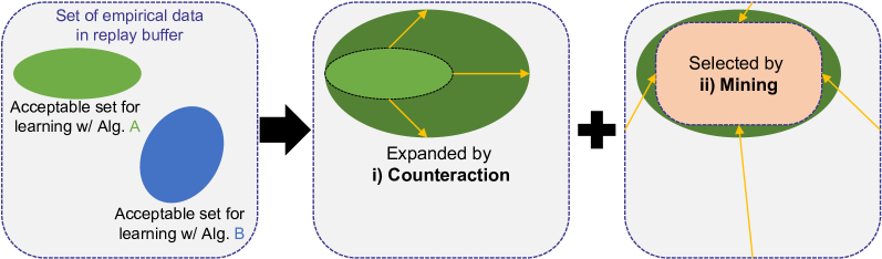
Figure 1: Concept of two stabilization tricks for satisfying ERC

To alleviate the identified instability factors, the two corresponding stabilization tricks, counteraction and mining, are proposed based on an experience discriminator. For the hypothesized ERC, i) the counteraction is responsible for expanding the acceptable set of empirical data, and ii) the mining is responsible for selectively replaying the empirical data belonging to it (see Fig. 1). Hence, ERC should hold by setting the appropriate counteraction and mining.

With the proposed stabilization tricks, it is verified whether ER is applicable to an advantage actor-critic (A2C) [33], an on-policy algorithm, by satisfying ERC. First, a rough grid search of hyperparameters is performed to identify the range of counteraction and mining in which ERC holds. Second, ablation tests for the counteraction and mining with the found hyperparameters show the needs for both. Finally, the A2C with the proposed stabilization tricks is evaluated on more practical multi-dimensional tasks, suggesting the learning performance comparable to SAC, which is the state-of-the-art off-policy algorithm.

In summary, this paper contributes to the following three folds:

1. It is revealed that the reason why ER is limited to off-policy algorithms is due to the two instability factors associated with triplet loss hidden in the policy improvement algorithms.

2. The two stabilization tricks, the counteraction and mining, are developed to alleviate the instability factors respectively.

3. With the two stabilization tricks, A2C, an on-policy algorithm, can satisfy ERC and achieve learning performance comparable to SAC.

2 Preliminaries

2.1 Basics of reinforcement learning

Let’s briefly introduce a problem statement for RL [46]. RL aims to maximize the sum of future rewards, so-called return, under Markov decision process (MDP). Mathematically, MDP is defined with the tuple $(\mathcal{S},\mathcal{A},p_{e},r)$: $\mathcal{S}$ and $\mathcal{A}$ denote the state and action spaces, respectively; $p_{e}:\mathcal{S}\times\mathcal{A}\mapsto\mathcal{S}$ gives the stochastic state transition function; and $r:\mathcal{S}\times\mathcal{A}\mapsto\mathcal{R}$ defines the reward function for the current situation with $\mathcal{R}\subset\mathbb{R}$ the set of rewards.

Under the above MDP, an agent encounters the current state $s_{t}\in\mathcal{S}$ of an (unknown) environment at the current time step $t\in\mathbb{N}$. The agent decides its action $a_{t}\in\mathcal{A}$ according to its learnable policy $\pi(a_{t}\mid s_{t}):\mathcal{S}\mapsto\mathcal{A}$. By interacting with the environment by $a_{t}$, the agent enters the next state $s_{t+1}=:s_{t}^{\prime}\in\mathcal{S}$ according to $p_{e}(s_{t}^{\prime}\mid s_{t},a_{t})$. At the same time, the reward $r_{t}=r(s_{t},a_{t})$ is obtained from the environment.

By repeating the above transition, the agent obtains the return, $R_{t}=\sum_{k=0}^{\infty}\gamma^{k}r_{t+k}$, with $\gamma\in[0,1)$ the discount factor. RL wants to maximize the expected return from $t$ by optimizing $\pi(a_{t}\mid s_{t})$ as follows:

$$\pi^{\ast}(a_{t}\mid s_{t})=\arg\max_{\pi}\mathbb{E}_{a_{t}\sim\pi(a_{t}\mid s_{t}),\tau_{t}\sim\rho^{\pi}}[R_{t}\mid s_{t}]$$ (1)

where $\rho^{\pi}$ denotes the probability to generate the state-action trajectory, $\tau_{t}=[s_{t}^{\prime},a_{t+1},\ldots]$, under $\pi$ and $p_{e}$. Here, the expected return can be defined as the following learnable value functions.

$$V(s_{t}) =\mathbb{E}_{a_{t}\sim\pi(a_{t}\mid s_{t}),\tau_{t}\sim\rho^{\pi}}[R_{t}\mid s_{t}]$$ (2)

$$Q(s_{t},a_{t}) =\mathbb{E}_{\tau_{t}\sim\rho^{\pi}}[R_{t}\mid s_{t},a_{t}]$$ (3)

where $V(s_{t})=\mathbb{E}_{a_{t}\sim\pi(a_{t}\mid s_{t})}[Q(s_{t},a_{t})]$ holds. The value functions are useful in acquring $\pi^{\ast}$, and therefore, most RL algorithms learn them.

2.2 RL algorithms with experience replay

ER stores the empirical data, $(s,a,s^{\prime},r,b)$ ($b=\pi(a\mid s)\in\mathbb{R}_{+}$ the policy likelihood to generate $a$, which is used for the proposed method), in a replay buffer $\mathcal{B}$ with finite size $|\mathcal{B}|$ in FIFO format [31]. For the sake of simplicity, this paper focuses on ER for learning algorithms with each single transition, although ER for long-term sequences has also been developed [17, 20]. That is, the loss function w.r.t. the learnable functions in RL (i.e. $\pi$, $V$, and/or $Q$ mainly) to be minimized can be computed for each empirical data. The following minimization problem is therefore given under ER.

$$\min_{f}\mathbb{E}_{(s,a,s^{\prime},r,b)\sim\mathcal{B}}[\ell_{f}^{\mathrm{alg}}(s,a,s^{\prime},r,b)]$$ (4)

where $f$ indicates the function(s) to be optimized and $\ell_{f}^{\mathrm{alg}}$ denotes the algorithm-dependent loss function for $f$ (even if other functions are used for computing it, they are not optimized through minimizing it).

2.2.1 Soft actor-critic

Here, two algorithms used in this paper are introduced briefly. The first one is SAC [14], which is known as a representative off-policy algorithm, as the comparison. SAC learns two functions, $\pi$ and $Q$, through minimization of the following loss functions .

$$\ell_{Q}^{\mathrm{SAC}}(s,a,s^{\prime},r) =\frac{1}{2}\{r+\gamma\mathbb{E}_{a^{\prime}\sim\pi(a^{\prime}\mid s^{\prime})}[\bar{Q}(s^{\prime},a^{\prime})-\alpha\ln\pi(a^{\prime}\mid s^{\prime})]-Q(s,a)\}^{2}$$ (5)

$$\ell_{\pi}^{\mathrm{SAC}}(s) =\mathbb{E}_{a\sim\pi(a\mid s)}[-Q(s,a)+\alpha\ln\pi(a\mid s)]$$ (6)

where $\bar{Q}$ denotes the target value (without computational graph) and $\alpha\geq 0$ denotes the magnitude of policy entropy, which can be auto-tuned by Kobayashi [27]. The two expectations w.r.t. $\pi$ are roughly approximated by a one-sample Monte Carlo method.

As for the optimization of $Q$, the expected SARSA [49], which can be an off-policy algorithm, is employed. Indeed, the target value of $Q$ is computed with $\pi$, which is different from the policy used for obtaining the empirical data (so-called the behavior policy). In addition, the optimization of $\pi$ is off-policy as well since $Q$ to be minimized in $\ell_{\pi}$ can be dependent on arbitrary policies (as like Lillicrap et al [30]). In this way, SAC belongs to the off-policy algorithm in total. As a result, SAC can optimize $\pi$ and $Q$ with arbitrary empirical data, making it possible to use ER freely.

2.2.2 Advantage actor-critic

Next, A2C [33], an on-policy algorithm, is introduced as the baseline for the proposed method. In this paper, the advantage function is approximated by the temporal difference (TD) error $\delta$ for simplicity. In other words, A2C in this paper learns $\pi$ and $V$ by minimizing the following loss functions.

$$\delta(s,s^{\prime},r) =r+\gamma\bar{V}(s^{\prime})-V(s)$$

$$\ell_{V}^{\mathrm{A2C}}(s,s^{\prime},r) =\frac{1}{2}\delta(s,s^{\prime},r)^{2}$$ (7)

$$\ell_{\pi}^{\mathrm{A2C}}(s,a,s^{\prime},r) =-\delta(s,s^{\prime},r)\ln\pi(a\mid s)$$ (8)

where $\bar{V}$ denotes the target value as like $\bar{Q}$.

As $V$ necessarily depends on $\pi$ by definition, the above learning rule for $V$ requires $\pi$-dependent $r$ (and $s^{\prime}$). The learning rule for $\pi$ is also derived based on the policy gradient theorem, and again the dependence of $\pi$ is assumed for $V$. In this way, A2C belongs to the on-policy algorithm in total. As a result, A2C should not be theoretically able to learn with ER, which stores the empirical data independent of $\pi$. Note that the policy gradient algorithm is theoretically converted to the off-policy algorithm by utilizing importance sampling [8], but due to computational instability and distribution shift, various countermeasures must be implemented [52, 57, 9] (see Section 6.1 in details).

2.3 Metric learning with triplet loss

Metric learning [3] is a methodology for extracting an embedding space, in which the similarity of the input data $x\in\mathcal{X}$ (e.g. image) can be measured. The triplet loss relevant to this study [50], which is one of the loss functions to extract the embedding space $\mathcal{Z}$, is briefly introduced. Three types of the input data, the anchor, positive, and negative data ($x$, $x^{+}$, and $x^{-}$ respectively), are required to compute it. These are fed into the common networks $f$, outputting the corresponding features in $\mathcal{Z}$. A distance function $d:\mathcal{Z}\times\mathcal{Z}\mapsto\mathbb{R}_{+}$ is then prepared to learn the desired distance relationship in the inputs. That is, $x$ should be close to $x^{+}$ and away from $x^{-}$, as shown in Fig. 2.

By minimizing the following triplet loss, this relationship can be acquired.

$$\ell_{f}^{\mathrm{triplet}}=\max(0,d(x,x^{+})+m-d(x,x^{-}))$$ (9)

where $m\geq 0$ denotes the margin between the positive and negative clusters. The max operator is applied to prevent divergence into negative infinity. That is, the anchor data can be embedded near the positive data while being away from the negative data to some extent.

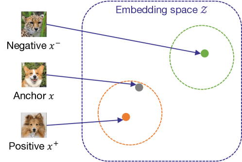
Figure 2: Desired distance relationship in metric learning with triplet loss

3 Reasons for instabilization by experience replay

3.1 Policy improvements via control as inference

CaI has been proposed for a new interpretation of RL [29]. To indicate that the policy improvements (e.g. A2C) can be regarded as a kind of triplet loss, CaI is utilized as below (see Kobayashi [24] for the details of derivation).

In this concept, an optimal variable $O=\{0,1\}$ is introduced. The probability mass functions, $p(O=1\mid s)$ and $p(O=1\mid s,a)$, can be defined with $V$ and $Q$, respectively.

$$p(O=1\mid s) =e^{\beta(V(s)-C)}=:p_{V}(s)$$ (10)

$$p(O=1\mid s,a) =e^{\beta(Q(s,a)-C)}=:p_{Q}(s,a)$$ (11)

where $\beta>0$ denotes the inverse temperature parameter. For convenience, $C$, which is numerically unknown, is substracted to satisfy $V(s)-C\leq 0$ and $Q(s,a)-C\leq 0$. Note that since $O$ is binary, the probability of $O=0$ can be given as $p(O=0\mid s)=1-p_{V}(s)$ and $p(O=0\mid s,a)=1-p_{Q}(s,a)$.

Using these probabilities, the optimal and non-optimal policies are inferred using Bayesian theorem. That is, $\pi(a\mid s,O)$ is given as follows:

$$\pi(a\mid s,O) =\cfrac{p(O\mid s,a)b(a\mid s)}{p(O\mid s)}$$

$$=\begin{cases}\cfrac{p_{Q}(s,a)}{p_{V}(s)}b(a\mid s)=:\pi^{+}(a\mid s)&O=1\\ \cfrac{1-p_{Q}(s,a)}{1-p_{V}(s)}b(a\mid s)=:\pi^{-}(a\mid s)&O=0\end{cases}$$ (12)

where $b(a\mid s)$ denotes the behavior policy to sample $a$, which can be different from the current learnable policy $\pi$.

Now, to optimize $\pi$, the following minimization problem is solved.

$$\min_{\pi}\mathbb{E}_{s\sim\mathcal{S}}[\mathrm{KL}(\pi(a\mid s)\mid\pi^{+}(a\mid s))-\mathrm{KL}(\pi(a\mid s)\mid\pi^{-}(a\mid s))]$$ (13)

where $\mathrm{KL}(\cdot\mid\cdot)$ denotes Kullback-Leibler (KL) divergence. The gradient of these two terms w.r.t. $\pi$, $g_{\pi}$, is derived as follows:

$$g_{\pi} =\mathbb{E}_{s\sim\mathcal{S}}\left[\nabla\mathbb{E}_{a\sim\pi(a\mid s)}\left[\ln\cfrac{\pi(a\mid s)}{\pi^{+}(a\mid s)}-\ln\cfrac{\pi(a\mid s)}{\pi^{-}(a\mid s)}\right]\right]$$

$$=\mathbb{E}_{s\sim\mathcal{S},a\sim\pi(a\mid s)}\left[-\nabla\ln\pi(a\mid s)\left\{\beta(Q(s,a)-V(s))+\ln\cfrac{1-p_{Q}(s,a)}{1-p_{V}(s)}\right\}\right]$$

$$\propto\mathbb{E}_{(s,a)\sim\mathcal{B}}\left[-(Q(s,a)-V(s))\nabla\ln\pi(a\mid s)\right]$$

$$\propto\mathbb{E}_{(s,a,s^{\prime},r)\sim\mathcal{B}}\left[-\delta(s,s^{\prime},r)\nabla\ln\pi(a\mid s)\right]$$ (14)

Here, by assuming $\beta\to\infty$, this gradient can be simplified. In addition, $Q-V=A$ the advantage function can be approximated by TD error $\delta$ (see Section 2.2.2).

It can be seen that the minimization of eq. (13) using the surrogated gradient is consistent with the minimization of the A2C loss function $\ell_{\pi}^{\mathrm{A2C}}$ by (stochastic) gradient descent. The original minimization problem can be interpreted as trying to move the anchor data $\pi$ closer to the positive data $\pi^{+}$ and away from the negative data $\pi^{-}$ by employing KL divergence as the distance function $d$ . Compared to eq. (9), the margin $m$ and the max operator are not used, but this is because $m=0$ and $\pi^{+,-}$ is centered on $b$, preventing the divergence to infinity.

3.2 Instability factors hidden in triplet loss

As the policy improvements correspond to minimizing triplet loss, then its characteristics during learning should also inherit that of minimizing triplet loss. Ideally, the anchor data should approach the positive data, resulting in $\pi\to\pi^{+}$. On the other hand, minimization of triplet loss is different from simple supervised learning, and several factors that destabilize learning have been reported. This study assumes that these instability factors become apparent in the policy improvements combined with ER. In this paper, therefore, the following two instability factors are raised as ones that needs to be addressed.

First, with inappropriate selection of anchor, positive, and negative data, $\mathrm{KL}(\pi\mid\pi^{+})>\mathrm{KL}(\pi\mid\pi^{-})$ might be caused. In this case, the repulsion from $\pi^{-}$ is stronger than the attraction to $\pi^{+}$ and the optimal solution cannot be found, updating $\pi$ by the divergent behavior. This is known as hard negative [6, 54]. To alleviate this instability factor, the exclusion of hard-negative triplets and/or the regularization that suppresses the repulsion would be required.

Second, from all the triplets that can be constructed, only a few can be used for optimization. In fact, $\pi^{+}$ and $\pi^{-}$ are linked via the behavior policy $b$ in the policy improvements, and no arbitrary triplet can be constructed. This causes distribution shift, inducing a large bias in learning [41, 55]. To alleviate this instability factor, it is desirable to eliminate triplets that are prone to bias and/or to regularize the distribution of selected triplets.

4 Tricks for experience replayable conditions

4.1 Experience discriminator

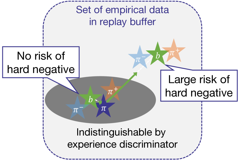
(a) Counteraction

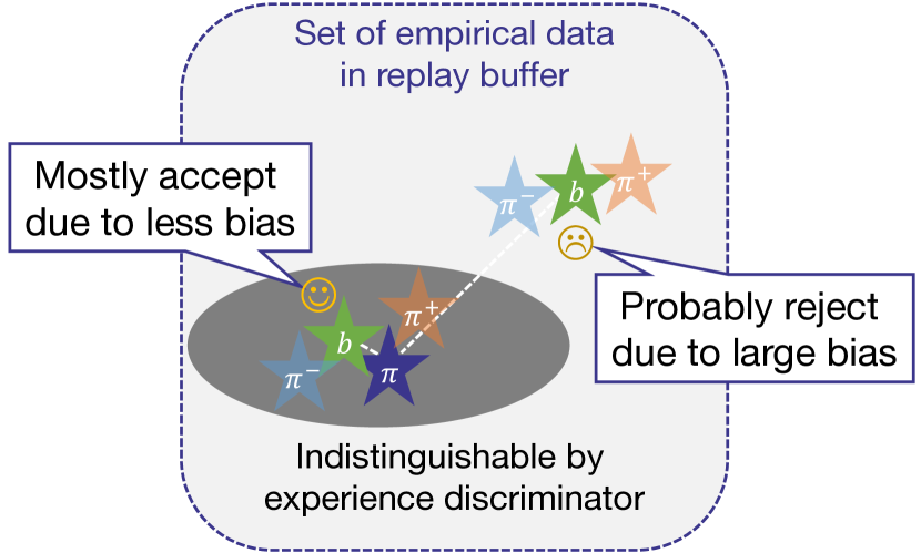
(b) Mining

Figure 3: Two stabilization tricks

The instability factors induced by the above triplet loss have to be suppressed to satisfy ERC. To this end, two stabilization tricks, counteraction and mining, are heuristically designed (see Fig. 3). As a common module for them, experience discriminator, is first introduced.

Specifically, it is required to judge whether the state-action pair $(s,a)$ in the buffer $\mathcal{B}$ can be regarded as one generated by the current policy $\pi$. According to the density trick, the following density ratio $d$ satisfies this requirement.

$$d(s,a,b) =\min\left(0.5,\cfrac{\pi(a\mid s)}{\pi(a\mid s)+b}\right)$$

$$=\min(0.5,\sigma(\ln\pi(a\mid s)-\ln b))$$ (15)

where $\sigma(\cdot)\in[0,1]$ is the sigmoid function. Note that $d$ should be equal to or less than $0.5$ since $(s,a)$ is actually generated from the behavior policy with likelihood $b$.

In addition, robust judgements should be considered w.r.t. the stochasticity of actions and the non-stationarity of policies. For this purpose, $D:\mathcal{S}\mapsto[0,1]$, which marginalizes $d$ by $a$ and has only $s$ as input, is defined as a learnable model. As $D$ corresponds to the probability parameter of Bernoulli distribution, it can be optimized through minimization of its negative log-likelihood.

$$\mathcal{L}_{D}=\mathbb{E}_{(s,a,b)\sim\mathcal{B}}[-d(s,a,b)\ln D(s)-(1-d(s,a,b))\ln(1-D(s))]$$ (16)

where the above $d$ is employed as the supervised signal.

4.2 Counteraction of deviations from non-optimal policies

First trick, so-called the counteraction, is proposed as a countermeasure against the hard negative mainly. In the previous work [6], the regularization to change the ratio of two terms in eq. (9) has been proposed to counteract the repulsion from the negative data. This concept can be reproduced in eq. (13) as follows:

$$\min_{\pi}\mathbb{E}_{s\sim\mathcal{S}}[(1+\lambda)\mathrm{KL}(\pi(a\mid s)\mid\pi^{+}(a\mid s))-\mathrm{KL}(\pi(a\mid s)\mid\pi^{-}(a\mid s))]$$ (17)

where, $\lambda\geq 0$ denotes the gain for imbalancing the positive and negative terms .

Now, how this extension works in practice is shown. As in the original minimization problem, the gradient for the added regularization is derived as below.

$$\nabla\mathbb{E}_{s\sim\mathcal{S}}[\mathrm{KL}(\pi(a\mid s)\mid\pi^{+}(a\mid s))]$$

$$= \nabla\mathbb{E}_{s\sim\mathcal{S},a\sim\pi}[\ln\pi(a\mid s)-\ln b(a\mid s)-\ln p_{Q}(s,a)+\ln p_{V}(s)]$$

$$= \nabla\mathbb{E}_{s\sim\mathcal{S}}[\mathrm{KL}(\pi(a\mid s)\mid b(a\mid s))]-\nabla\mathbb{E}_{s\sim\mathcal{S},a\sim\pi}[\ln p_{Q}(s,a)-\ln p_{V}(s)]$$ (18)

Now, the second term can be decomposed to eq. (14) by using the definitions of $p_{V}$ and $p_{Q}$ in eqs. (10) and (11), respectively.

$$-\nabla\mathbb{E}_{s\sim\mathcal{S},a\sim\pi}[\ln p_{Q}(s,a)-\ln p_{V}(s)]$$

$$= -\nabla\mathbb{E}_{s\sim\mathcal{S},a\sim\pi}[\beta Q(s,a)-\beta C-\beta V(s)+\beta C]$$

$$= \mathbb{E}_{s\sim\mathcal{S},a\sim\pi}[-\nabla\ln\pi(a\mid s)\beta\{Q(s,a)-V(s)\}]$$

$$\propto \mathbb{E}_{(s,a,s^{\prime},r)\sim\mathcal{B}}\left[-\delta(s,s^{\prime},r)\nabla\ln\pi(a\mid s)\right]=\eqref{eq:cai_a2c}$$ (19)

That is, the second term can be absorbed into the original loss.

The added regularization, therefore, has a role to constrain $\pi\to b$ only. As $b$ should be located between $\pi^{+}$ and $\pi^{-}$, this regularization is expected to avoid the hard negative and stabilize $\pi\to\pi^{+}$. However, to implement this regularization directly, the behavior policy $b(a\mid s)$ at each experience must be retained, which is costly. As an alternative regularization way, the adversarial learning to eq. (16) is implemented in this paper.

That is, it takes advantage of the fact that the higher the misidentification rate of $D$ means $\pi\sim b$, reducing the risk of hard negative (see Fig. 3(a)). Since $d$ has the computational graph w.r.t. $\pi$, the following loss function can be given as the counteraction trick for regularizing $\pi$ to $b$.

$$\mathcal{L}_{C}=\mathbb{E}_{(s,a,b)\sim\mathcal{B}}[\omega d(s,a,b)\{\ln D(s)-\ln(1-D(s))\}]$$ (20)

where, $\omega\geq 0$ denotes the gain, which is designed below. One can find that the term related to $D$ also behaves as a gain and is larger when $D\ll 1$ (i.e. no misidentification). In addition, if $d$ is clipped to $0.5$ (i.e. $\pi\simeq b$ holds), the gradient w.r.t. $\pi$ is zero. Note that, in the actual implementation, the gradient reversal layer [12] is useful to lump eqs. (16) and (20) together.

As for $\omega$, $d\ll 1$ has the small gradient due to the sigmoid function, not like $D\ll 1$. To compensate it and improve convergence performance to $\pi\to b$ even in such a case, $\omega$ is designed in the manner of PI control, referring to the literature [45].

$$\begin{split}P(s,a,b)&=\eta_{C}(1-2\hat{d}(s,a,b))\\ I&=\max(0,0.5I+\mathbb{E}_{\mathcal{B}}[P(s,a,b)])\\ \omega(s,a,b)&=\max(0,P(s,a,b)+I)\end{split}$$ (21)

where $\hat{d}$ means $d$ without the computational graph, and $\eta_{C}\geq 0$ denotes the hyperparameter for this counteraction. $I\geq 0$ is the integral term with saturation by multiplying $0.5$ (its initial value must be zero).

4.3 Mining of indistinguishable experiences

Second trick, so-called the mining, is proposed to mitigate the effect of distribution shift mainly. In previous studies, semi-hard triplets, which satisfy $d(x,x^{+})+m<d(x,x^{-})$, are considered useful [41]. Since the optimization problem in this study sets $m=0$, $\mathrm{KL}(\pi\mid\pi^{+})<\mathrm{KL}(\pi\mid\pi^{-})$ seems better. However, this is also regarded to be hard triplets, which would induce selection bias. Of course, $\mathrm{KL}(\pi\mid\pi^{+})>\mathrm{KL}(\pi\mid\pi^{-})$ is still not suitable for learning because of the hard negative relationship described above. Hence, the triplets with $\mathrm{KL}(\pi\mid\pi^{+})\simeq\mathrm{KL}(\pi\mid\pi^{-})$ are desired to be mined.

Specifically, it takes advantage of the fact that, in this study, the anchor data is determined by the current policy $\pi$, and the positive and negative data, $\pi^{+}$ and $\pi^{-}$, are located around the behavior policy $b$. In other words, the indistinguishable empirical data with $\pi\simeq b$ is likely to achieve the desired relationship (see Fig. 3(b)). The mining trick is therefore given as the following stochastic dropout [44].

$$\begin{split}p(M\mid s,a,b)&=2\max(0,0.5-\min(d(s,a,b),D(s))^{\eta_{M}})\\ M&=\begin{cases}1&p(M\mid s,a,b)\leq\epsilon\sim\mathcal{U}(0,1)\\ 0&\text{otherwise}\end{cases}\end{split}$$ (22)

where $\mathcal{U}(l,u)$ is the uniform distribution within $[l,u]$, and $\eta_{M}\geq 0$ denotes the hyperparameter for this mining. When sampling the empirical data from the replay buffer $\mathcal{B}$, each data is screend by the mining: if $M=1$, it is used for the optimization; if $M=0$, it is excluded.

5 Simulations

5.1 Overview

Here, it is verified that ERC is satisfied by the two stabilization tricks. To do so, A2C [33], which is the on-policy algorithm and generally considered inapplicable for ER, is employed as a baseline (see Appendix A for detailed settings). Learning is conducted only with the empirical data replayed from ER at the end of each episode (without online learning).

The following three steps are performed for the step-by-step verification. With them, it is shown that alleviating the instability factors hidden in triplet loss is effective not only to satisfy ERC, but also to learn with comparable sample efficiency to SAC [14].

1. The hyperparameters of the respective stabilization tricks, $\eta_{C,M}\geq 0$, are roughly examined their effective ranges in a toyproblem, determining the values to be used in the subsequent verification.

2. It is confirmed that both of the two stabilization tricks are complementarily essential to satisfy ERC and to learn the optimal policy through ablation tests on three major tasks implemented in Mujoco [47].

3. Finally, A2C with the proposed stabilization tricks is evaluated on two tasks of relatively large problem scale in dm_control [48] in comparison to SAC, which is the latest off-policy algorithm.

Note that training for each task and condition is conducted 12 times with different random seeds in order to evaluate the performance with their statistics.

5.2 Effective range of hyperparameters

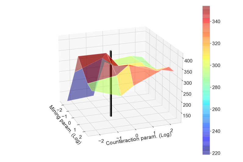
Figure 4: Grid search of $(\eta_{C},\eta_{M})$ on DoublePendulum

A toy problem named DoublePendulum, where a pendulum agent with two passive joints tries to balance in a standing position by moving its base, is solved. This has only one-dimensional action space and the state space limited by a terminal condition (i.e. excessive tilting). Thus, as this is a relatively simple problem and many empirical data should naturally satisfy ERC, the effect of $\eta_{C,M}$ should behave in a Gaussian manner, enabling adjustment statistically.

To roughly check the effective parameter ranges of $\eta_{C,M}$, $5\times 5=25$ conditions with $\eta_{C,M}=\{0.1,0.5,1.0,5.0,10.0\}$ are compared. The test results, which are evaluated after learning, are summarized in Fig. 4. The results suggest the following two points.

First, $\eta_{M}$ must be of a certain scale to activate the selection of empirical data, or else the performance can be significantly degraded. However, an excessively large $\eta_{M}$ would result in too little empirical data being replayed. Therefore, $\eta_{M}$ is considered reasonable in the vicinity of $1$.

Second, $\eta_{C}$ seems to have an appropriate range depending on $\eta_{M}$. In other words, if $\eta_{M}$ is excessively large and the replayable empirical data is too limited, it is desirable to increase them by increasing $\eta_{C}$. On the other hand, if the empirical data are moderately selected around $\eta_{M}\simeq 1$, it seems essential to relax the counteraction to some extent as $\eta_{C}\leq 1$.

Based on the two trends, and as a natural setting, $(\eta_{C},\eta_{M})$ are decided to be $(0.5,2.0)$. The learning performance at this time is also shown in Fig. 4 (the black bar), and is higher than the rough grid search results (i.e. $\sim 416$ while the others did not exceed $400$).

5.3 Ablation tests

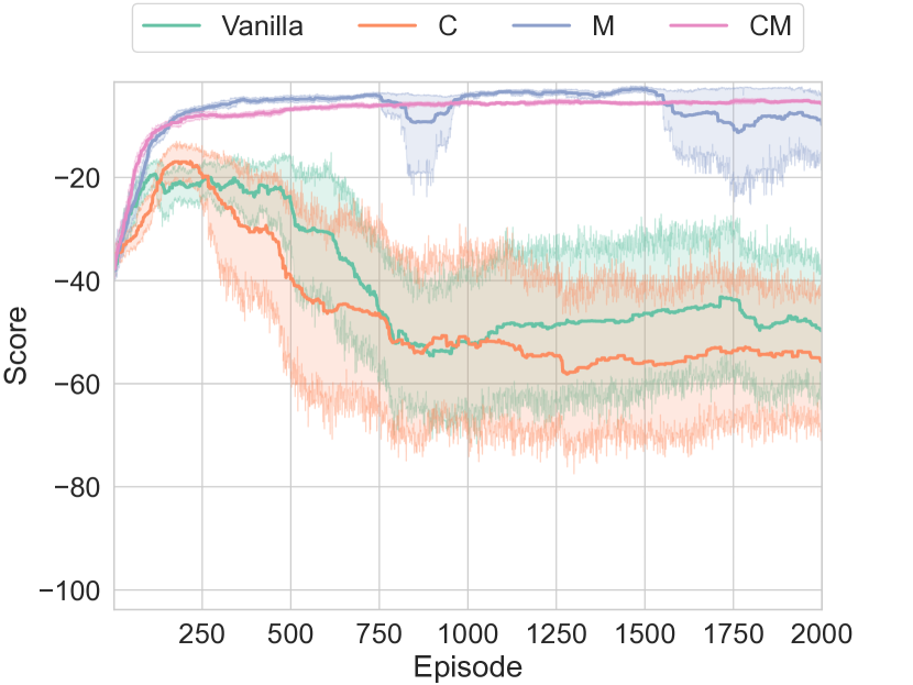
(a) Reacher

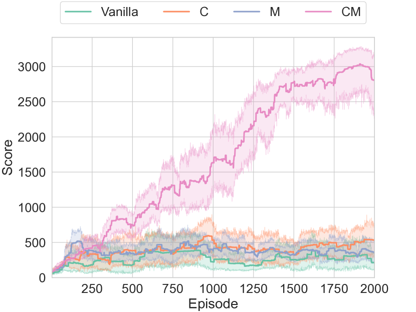
(b) Hopper

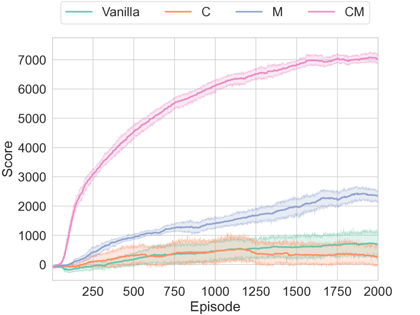
(c) HalfCheetah

Figure 5: Returns of ablation tests

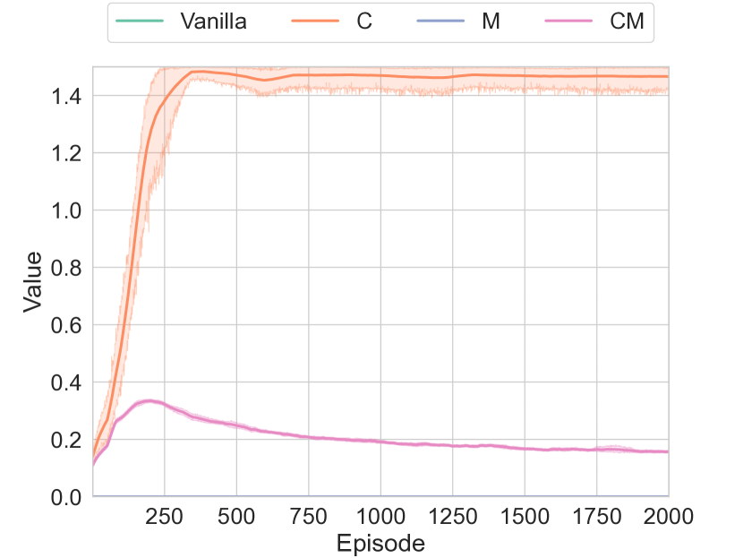
(a) Reacher

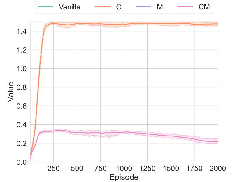
(b) Hopper

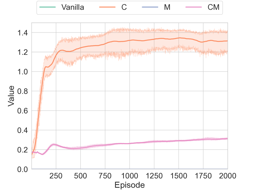
(c) HalfCheetah

Figure 6: $\omega(s,a,b)$ in the counteraction trick

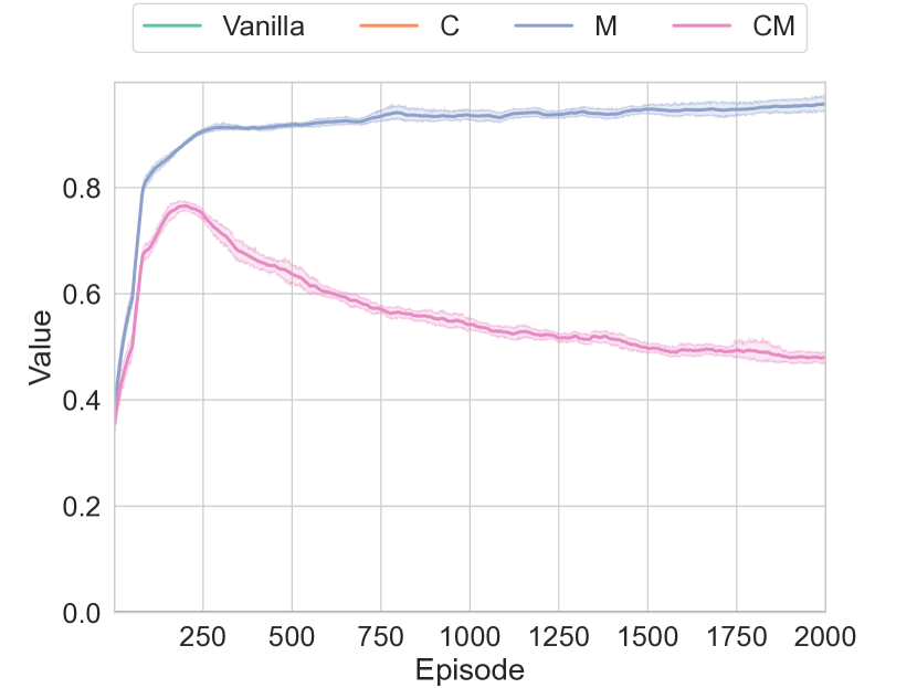
(a) Reacher

(b) Hopper

(c) HalfCheetah

Figure 7: $p(M\mid s,a,b)$ in the mining trick

Next, the needs for the two stabilization tricks are demonstrated through ablation tests. Specifically, the presence or absence of the two stabilization tricks (labeled with their initials ‘C’ and ‘M’) is switched by setting $\eta_{C,M}=0$. The four conditions of that combination are compared in the following three tasks in Mujoco [47]: Reacher; Hopper; and HalfCheetah.

The learning curves for these returns are shown in Fig. 5. As can be seen from the results, Vanilla (a.k.a. the standard A2C) without the two stabilization tricks did not learn any tasks at all, probably because it does not satisfy ERC. Adding the counteraction trick alone did not improve learning as well, but adding the mining trick improved somewhat. Nevertheless, it seems that either of them does not satisfy ERC or learn the optimal policy. On the other hand, only the case using the two stabilization tricks was able to learn all tasks. From these results, it can be concluded that both of the two stabilization tricks are necessary (and sufficient) to satisfy ERC and learn the optimal policy.

Now let’s see why both stabilization tricks are required. To this end, the internal parameters for the respective stabilization tricks, $\omega(s,a,b)$ and $p(M\mid s,a,b)$, are depicted in Figs. 6 and 7. One can find that the cases only with one of the stabilization tricks immediately saturated the respective internal parameters. That is, if using the counteraction trick only, its regularization to $\pi\to b$ is not enough for satisfying ERC; and if using the mining trick only, its selection is too strict for learning the optimal policy. On the other hand, by using both, the internal parameters converged to task-specific values without saturation. That is why the two stabilization tricks need to be used together to increase the amount of replayable empirical data to reach a level where the optimal policy can be learned while still satisfying ERC.

5.4 Performance comparison

Figure 8: Test results on practical tasks

Finally, the learning performance of the A2C with the proposed stabilization tricks (labeled ERC) is compared to the state-of-the-art off-policy algorithm, SAC [14]. Two practical tasks with more than 10-dimensional action space, QuadrupedWalk (with $|\mathcal{A}|=12$) and Swimmer15D (with $|\mathcal{A}|=14$) in dm_control [48], are solved.

The test results after learning are depicted in Fig. 8. As can be seen, while SAC solved Quadruped at a high level, it did not solve Swimmer consistently. On the other hand, ERC performed unstably on Quadruped, but showed high performance on Swimmer. Thus, it can be said that ERC has a learning performance comparable to that of SAC, although they have different strengths in different tasks.

As a remark, the difference in performance between ERC and SAC might be attributed to the difference in the policy gradients used. Actually, ERC learns the policy with likelihood-ratio gradients, while SAC does so with reparameterization gradients [37]. The former obtains the gradients over the entire (multi-dimensional) policy, which cannot optimize each component of actions independently. As a result, this is useful to learn tasks that require synchonization of actions. The latter, on the other hand, obtains the gradients for each component of actions, and thus can quickly learn tasks that do not require precise synchronization. These learning characteristics correspond to the two types of tasks solved in this study. Hence, it is suggested that SAC performed well for Quadruped, where synchronization at each leg is sufficient, and ERC performed well for Swimmer, where synchronization at all joints is needed. Note that policy improvements by mixing them have been proposed, which would be expected to be useful [13].

6 Discussions

6.1 Relations to conventional algorithms

As demonstrated in the above section, ERC hypothesized in this study can be achieved by limiting the replayed empirical data to ones acceptable by the applied RL algorithm. At the same time, the improvement in learning efficiency due to ER can be increased by expanding the acceptable set of empirical data. These were achieved by the two stabilization tricks proposed, with $\pi\simeq b$ being the key to both. This corresponds to the concept of on-policyness, where the empirical data contained in the replay buffer can be regarded as generated from the current policy $\pi$ [10]. In other words, the proposed stabilization tricks aimed to stabilize the triplet loss and consequently increased the on-policyness. Conversely, the usefulness of increasing the on-policyness in previous studies [34, 43] can be explained in terms of mitigating the instabilization factors hidden in the triplet loss.

Actually, ER can be applied to make A2C off-policy [8]. To this end, the most important trick is to change the sampler by importance sampling, as described above. This trick involves weighting the original loss function by $\pi/b$, which is unstable when $b\simeq 0$ (i.e. rare actions are sampled). Several heuristics have been proposed to resolve this instability [52, 57, 9]. On the other hand, the proposed stabilization tricks selectively replay the empirical data with $\pi\simeq b$ while increasing the number of acceptable ones. As a result, the weight in this important sampling can be ignored as $\pi/b\simeq 1$. That is why A2C with the proposed stabilization tricks, although not explicitly off-policy, made ER available as if they were off-policy.

As a remark, the report that PPO (and its variants), which is on-policy [42], could utilize ER empirically [26] is related to the above considerations and the proposed stabilization tricks. That is, PPO applies regularization aiming at $\pi\simeq b$, and if $\pi$ deviates from $b$, it clips the weight of the importance sampling, resulting in excluding that data. Thus, PPO can increase the on-policyness of empirical data and exclude from replays that are unacceptable, so ER is actually applicable.

Finally, another interpretation of why DDPG [30], SAC [14], and TD3 [11], which are considered off-policy, can stably learn the optimal policy using ER. These algorithms optimize the current policy $\pi$ by using reparameterization gradients through the actions generated from $\pi$ fed into the action value function $Q$. As mentioned in the SAC paper, this can be derived from the minimization of KL divergence between $\pi$ and the optimal policy based on $Q$ only. In other words, unlike algorithms that use likelihood-ratio gradients such as A2C, they do not deal with the triplet loss. Therefore, it can be considered that ER is applicable since there is no instabilization factors induced by the triplet loss in the first place.

6.2 Limitations of stabiliation tricks

For ERC holding, this paper proposed the two stabilization tricks, the contributions of which were evaluated in the above section. However, these naturally leave room for improvements. First, using them requires a discriminator $D$ learned through eq. (16), which needs an extra computational cost. While it is possible to implement the two tricks using only $d$ in eq. (15) without $D$, $d$ is an unstable variable, so a lightweight stabilizer will be needed to replace $D$.

It is also important to note that the decision on $D$ and $d$ is based on the likelihood $\pi$ and $b$. That is, when the policy deals with a high-dimensional action space, even a small deviation in action may be judged as $\pi\neq b$ severely. In fact, when the RL benchmark with musculoskeletal model, i.e. myosuite [4], was tested with $|\mathcal{A}|=39$, $p(M\mid s,a,b)$ often converged to one depending on the conditions. This means that most of the empirical data could not be replayed. To avoid this excessive exclusion of empirical data, it would be useful to either determine the final exclusion of empirical data by summarizing the respective judgements on individual action dimension separately; or to optimize the policy by masking the inappropriate action dimension only.

In addition, the counteraction alone did not satisfy ERC, as indicated in the ablation tests. This is probably due to saturation of the regularization gain $\omega$ (see Fig. 6). Although a non-saturated gain made learning unstable empirically, it would be better to relax the saturation to some extent. Alternatively, an auto-tuning trick, which is possible by once interpreting the regularization as the constraint [15, 27], is considered to be useful.

7 Conclusion

This study reconsidered the factors that cause whether ER is applicable to RL algorithms. To this end, the instability factors that ER might induce especifally in on-policy algorithms were first revealed. In other words, it was found that the policy gradient algorithms can be regarded as the minimization of triplet loss in metric learning, inheriting its instability factors. To alleviate them, the two stabilization tricks, the counteraction and mining, were proposed as countermeasures attached to arbitrary RL algorithms. The counteraction and mining are responsible for i) expanding the set of acceptable empirical data for each RL algorithm and ii) excluding empirical data outside the set, respectively. Through multiple simulations, ERC indeed holded by using these two stabilization tricks. Furthermore, the standard on-policy algorithm with them achieved the learning performance comparable to the state-of-the-art off-policy algorithm.

As described in the discussion, the two stabilization tricks proposed to satisfy ERC leave some room for improvements. In particular, since the hypothesis formulated in this study is now deeply related to the on-policyness of the empirical data in the replay buffer, they would be improved based on this perspective. Afterwards, other RL algorithms will be integrated with the stabilization tricks for further investigations of ERC.

Acknowledgments

This research was supported by “Strategic Research Projects” grant from ROIS (Research Organization of Information and Systems).

Data Availability

The datasets generated during and/or analyzed during the current study are available from the corresponding author on reasonable request.

Competing interests

The author declares that there is no known competing financial interests or personal relationships that could have appeared to influence the work reported in this paper.

Appendix A Details of implementation

The algorithms used in this paper is implemented with Pytorch [38]. This implementation is based on the one in the literature [25]. The characteristic hyperparameters in this implementation are listed up in Table 1.

The policy and value functions are approximated by a fully-connected neural networks consisting of two hidden layers with 100 neurons for each. As activation functions, Squish function [1, 28] and RMSNorm [56] are combined. AdaTerm [18], which is the noise-robust optimizer, is adopted for robustly optimizing parameters against noises caused by bootstrapped learning in RL. Similarly, target networks that are updated by CAT-soft update [22] are employed to stabilize learning (and to prevent learning speed degradation). In A2C, the target networks is applied to both the policy $\pi$ and the value function $V$, while in SAC they are applied only to the action value function $Q$. In addition, A2C enhances output continuity by using L2C2 [23] with default parameters, although SAC does not so due to reproduction of its standard implementation.

Both A2C and SAC policies are modeled as Student’s t-distribution with high global exploration capability [21]. Therefore, the outputs from the networks are three model parameters: position, scale, and degrees of freedom. However, as in the standard implementation of SAC, the process of converting the generated action to a bounded range is also explicitly considered as a probability distribution. On the other hand, in A2C, this process is performed implicitly on the environment side and is not reflected in the probability distribution.

SAC approximates the two action value functions $Q_{1,2}$ with independent networks as in the standard implementation, and aims at conservative learning by selecting the smaller value. On the other hand, A2C aims at stable learning by outputting 10 values from shared networks and using the median as the representative value. In order to enhance the effect of ensemble learning, the outputs are computed with both learnable and unlearnable parameters, so that each output can easily take on different values (especially in unlearned regions) [36].

A2C and SAC share the settings of ER, with a buffer size of 102,400 and a batch size of 256. The replay buffer is in FIFO format that deletes the oldest empirical data when the buffer size is exceeded. At the end of each episode, half of the empirical data stored in ER is replayed uniformly at random.

Table 1: Parameter configuration

Symbol	Meaning	Value
–	#Hidden layers	$2$
–	#Neurons for each hidden layer	$100$
–	Activation function	Squish + RMSNorm
$\gamma$	Discount factor	$0.99$
$\alpha$	Learning rate for AdaTerm	$10^{-3}$
$\tau$	Update rate of target networks	$0.1$
$|\mathcal{B}|$	Buffer size	$102400$
$N_{b}$	Batch size	$256$
$N_{r}$	#Replayed data	$|\mathcal{B}|/2$

References

- \bibcommenthead
- Barron [2021] Barron JT (2021) Squareplus: A softplus-like algebraic rectifier. arXiv preprint arXiv:211211687
- Bejjani et al [2018] Bejjani W, Papallas R, Leonetti M, et al (2018) Planning with a receding horizon for manipulation in clutter using a learned value function. 1803.08100
- Bellet et al [2022] Bellet A, Habrard A, Sebban M (2022) Metric learning. Springer Nature
- Caggiano et al [2022] Caggiano V, Wang H, Durandau G, et al (2022) Myosuite–a contact-rich simulation suite for musculoskeletal motor control. arXiv preprint arXiv:220513600
- Chen et al [2021] Chen J, Li SE, Tomizuka M (2021) Interpretable end-to-end urban autonomous driving with latent deep reinforcement learning. IEEE Transactions on Intelligent Transportation Systems 23(6):5068–5078
- Cheng et al [2016] Cheng D, Gong Y, Zhou S, et al (2016) Person re-identification by multi-channel parts-based cnn with improved triplet loss function. In: IEEE conference on computer vision and pattern recognition, pp 1335–1344
- Cui et al [2021] Cui Y, Osaki S, Matsubara T (2021) Autonomous boat driving system using sample-efficient model predictive control-based reinforcement learning approach. Journal of Field Robotics 38(3):331–354
- Degris et al [2012] Degris T, White M, Sutton RS (2012) Off-policy actor-critic. In: International Conference on Machine Learning
- Fakoor et al [2020] Fakoor R, Chaudhari P, Smola AJ (2020) P3O: Policy-on policy-off policy optimization. In: Uncertainty in Artificial Intelligence, PMLR, pp 1017–1027
- Fedus et al [2020] Fedus W, Ramachandran P, Agarwal R, et al (2020) Revisiting fundamentals of experience replay. In: International Conference on Machine Learning, PMLR, pp 3061–3071
- Fujimoto et al [2018] Fujimoto S, Hoof H, Meger D (2018) Addressing function approximation error in actor-critic methods. In: International conference on machine learning, PMLR, pp 1587–1596
- Ganin et al [2016] Ganin Y, Ustinova E, Ajakan H, et al (2016) Domain-adversarial training of neural networks. Journal of machine learning research 17(59):1–35
- Gu et al [2017] Gu SS, Lillicrap T, Turner RE, et al (2017) Interpolated policy gradient: Merging on-policy and off-policy gradient estimation for deep reinforcement learning. Advances in neural information processing systems 30
- Haarnoja et al [2018a] Haarnoja T, Zhou A, Abbeel P, et al (2018a) Soft actor-critic: Off-policy maximum entropy deep reinforcement learning with a stochastic actor. In: International conference on machine learning, PMLR, pp 1861–1870
- Haarnoja et al [2018b] Haarnoja T, Zhou A, Hartikainen K, et al (2018b) Soft actor-critic algorithms and applications. arXiv preprint arXiv:181205905
- Hambly et al [2023] Hambly B, Xu R, Yang H (2023) Recent advances in reinforcement learning in finance. Mathematical Finance 33(3):437–503
- Hansen et al [2018] Hansen S, Pritzel A, Sprechmann P, et al (2018) Fast deep reinforcement learning using online adjustments from the past. Advances in Neural Information Processing Systems 31
- Ilboudo et al [2023] Ilboudo WEL, Kobayashi T, Matsubara T (2023) Adaterm: Adaptive t-distribution estimated robust moments for noise-robust stochastic gradient optimization. Neurocomputing 557:126692
- Kalashnikov et al [2018] Kalashnikov D, Irpan A, Pastor P, et al (2018) Scalable deep reinforcement learning for vision-based robotic manipulation. In: Conference on Robot Learning, PMLR, pp 651–673
- Kapturowski et al [2019] Kapturowski S, Ostrovski G, Quan J, et al (2019) Recurrent experience replay in distributed reinforcement learning. In: International Conference on Learning Representations
- Kobayashi [2019] Kobayashi T (2019) Student-t policy in reinforcement learning to acquire global optimum of robot control. Applied Intelligence 49(12):4335–4347
- Kobayashi [2022a] Kobayashi T (2022a) Consolidated adaptive t-soft update for deep reinforcement learning. arXiv preprint arXiv:220212504
- Kobayashi [2022b] Kobayashi T (2022b) L2c2: Locally lipschitz continuous constraint towards stable and smooth reinforcement learning. In: IEEE/RSJ International Conference on Intelligent Robots and Systems, IEEE, pp 4032–4039
- Kobayashi [2022c] Kobayashi T (2022c) Optimistic reinforcement learning by forward kullback–leibler divergence optimization. Neural Networks 152:169–180
- Kobayashi [2023a] Kobayashi T (2023a) Intentionally-underestimated value function at terminal state for temporal-difference learning with mis-designed reward. arXiv preprint arXiv:230812772
- Kobayashi [2023b] Kobayashi T (2023b) Proximal policy optimization with adaptive threshold for symmetric relative density ratio. Results in Control and Optimization 10:100192
- Kobayashi [2023c] Kobayashi T (2023c) Soft actor-critic algorithm with truly-satisfied inequality constraint. arXiv preprint arXiv:230304356
- Kobayashi and Aotani [2023] Kobayashi T, Aotani T (2023) Design of restricted normalizing flow towards arbitrary stochastic policy with computational efficiency. Advanced Robotics pp 1–18
- Levine [2018] Levine S (2018) Reinforcement learning and control as probabilistic inference: Tutorial and review. arXiv preprint arXiv:180500909
- Lillicrap et al [2015] Lillicrap TP, Hunt JJ, Pritzel A, et al (2015) Continuous control with deep reinforcement learning. arXiv preprint arXiv:150902971
- Lin [1992] Lin LJ (1992) Self-improving reactive agents based on reinforcement learning, planning and teaching. Machine learning 8(3-4):293–321
- Mnih et al [2015] Mnih V, Kavukcuoglu K, Silver D, et al (2015) Human-level control through deep reinforcement learning. nature 518(7540):529–533
- Mnih et al [2016] Mnih V, Badia AP, Mirza M, et al (2016) Asynchronous methods for deep reinforcement learning. In: International conference on machine learning, PMLR, pp 1928–1937
- Novati and Koumoutsakos [2019] Novati G, Koumoutsakos P (2019) Remember and forget for experience replay. In: International Conference on Machine Learning, PMLR, pp 4851–4860
- Oh et al [2021] Oh I, Rho S, Moon S, et al (2021) Creating pro-level ai for a real-time fighting game using deep reinforcement learning. IEEE Transactions on Games 14(2):212–220
- Osband et al [2018] Osband I, Aslanides J, Cassirer A (2018) Randomized prior functions for deep reinforcement learning. Advances in Neural Information Processing Systems 31
- Parmas and Sugiyama [2021] Parmas P, Sugiyama M (2021) A unified view of likelihood ratio and reparameterization gradients. In: International Conference on Artificial Intelligence and Statistics, PMLR, pp 4078–4086
- Paszke et al [2019] Paszke A, Gross S, Massa F, et al (2019) Pytorch: An imperative style, high-performance deep learning library. Advances in neural information processing systems 32
- Saglam et al [2023] Saglam B, Mutlu FB, Cicek DC, et al (2023) Actor prioritized experience replay. Journal of Artificial Intelligence Research 78:639–672
- Schaul et al [2015] Schaul T, Quan J, Antonoglou I, et al (2015) Prioritized experience replay. arXiv preprint arXiv:151105952
- Schroff et al [2015] Schroff F, Kalenichenko D, Philbin J (2015) Facenet: A unified embedding for face recognition and clustering. In: IEEE conference on computer vision and pattern recognition, pp 815–823
- Schulman et al [2017] Schulman J, Wolski F, Dhariwal P, et al (2017) Proximal policy optimization algorithms. arXiv preprint arXiv:170706347
- Sinha et al [2022] Sinha S, Song J, Garg A, et al (2022) Experience replay with likelihood-free importance weights. In: Learning for Dynamics and Control Conference, PMLR, pp 110–123
- Srivastava et al [2014] Srivastava N, Hinton G, Krizhevsky A, et al (2014) Dropout: a simple way to prevent neural networks from overfitting. The journal of machine learning research 15(1):1929–1958
- Stooke et al [2020] Stooke A, Achiam J, Abbeel P (2020) Responsive safety in reinforcement learning by pid lagrangian methods. In: International Conference on Machine Learning, PMLR, pp 9133–9143
- Sutton and Barto [2018] Sutton RS, Barto AG (2018) Reinforcement learning: An introduction. MIT press
- Todorov et al [2012] Todorov E, Erez T, Tassa Y (2012) Mujoco: A physics engine for model-based control. In: IEEE/RSJ international conference on intelligent robots and systems, IEEE, pp 5026–5033
- Tunyasuvunakool et al [2020] Tunyasuvunakool S, Muldal A, Doron Y, et al (2020) dm_control: Software and tasks for continuous control. Software Impacts 6:100022
- Van Seijen et al [2009] Van Seijen H, Van Hasselt H, Whiteson S, et al (2009) A theoretical and empirical analysis of expected sarsa. In: IEEE symposium on adaptive dynamic programming and reinforcement learning, IEEE, pp 177–184
- Wang et al [2014] Wang J, Song Y, Leung T, et al (2014) Learning fine-grained image similarity with deep ranking. In: IEEE conference on computer vision and pattern recognition, pp 1386–1393
- Wang et al [2021] Wang X, Song J, Qi P, et al (2021) Scc: An efficient deep reinforcement learning agent mastering the game of starcraft ii. In: International conference on machine learning, PMLR, pp 10905–10915
- Wang et al [2017] Wang Z, Bapst V, Heess N, et al (2017) Sample efficient actor-critic with experience replay. In: International Conference on Learning Representations
- Wu et al [2023] Wu P, Escontrela A, Hafner D, et al (2023) Daydreamer: World models for physical robot learning. In: Conference on Robot Learning, PMLR, pp 2226–2240
- Xuan et al [2020] Xuan H, Stylianou A, Liu X, et al (2020) Hard negative examples are hard, but useful. In: European Conference on Computer Vision, pp 126–142
- Yu et al [2018] Yu B, Liu T, Gong M, et al (2018) Correcting the triplet selection bias for triplet loss. In: European Conference on Computer Vision, pp 71–87
- Zhang and Sennrich [2019] Zhang B, Sennrich R (2019) Root mean square layer normalization. Advances in Neural Information Processing Systems 32
- Zhang et al [2019] Zhang S, Boehmer W, Whiteson S (2019) Generalized off-policy actor-critic. Advances in neural information processing systems 32
- Zhao et al [2016] Zhao D, Wang H, Shao K, et al (2016) Deep reinforcement learning with experience replay based on sarsa. In: IEEE symposium series on computational intelligence, IEEE, pp 1–6