Planning with a Receding Horizon for Manipulation in Clutter
using a Learned Value Function

Abstract

Manipulation in clutter requires solving complex sequential decision making problems in an environment rich with physical interactions. The transfer of motion planning solutions from simulation to the real world, in open-loop, suffers from the inherent uncertainty in modelling real world physics. We propose interleaving planning and execution in real-time, in a closed-loop setting, using a Receding Horizon Planner (RHP) for pushing manipulation in clutter. In this context, we address the problem of finding a suitable value function based heuristic for efficient planning, and for estimating the cost-to-go from the horizon to the goal. We estimate such a value function first by using plans generated by an existing sampling-based planner. Then, we further optimize the value function through reinforcement learning. We evaluate our approach and compare it to state-of-the-art planning techniques for manipulation in clutter. We conduct experiments in simulation with artificially injected uncertainty on the physics parameters, as well as in real world tasks of manipulation in clutter. We show that this approach enables the robot to react to the uncertain dynamics of the real world effectively.

I Introduction

We propose a planning approach for physics-based manipulation in clutter, for tasks in which an object has to be pushed to a goal region, with little to no repositioning of other objects. Such robotic manipulation skills are required in a variety of applications. In service robotics, for example, robots have to simultaneously interact with multiple everyday objects (e.g., objects in drawers or in cabinets) to execute household activities [1, 2]. In industrial settings, such as in warehouses, robots have to fulfill orders by picking items off cluttered shelves, as in the Amazon Picking Challenge [3]. This requires pushing certain items out of the way, without dropping them off the shelf, while reaching for a target item.

There has been significant recent interest in motion planning for pushing-based manipulation tasks in clutter, and impressive planners have been proposed [4, 5, 6]. Real-world execution of these trajectories, however, still poses great challenges. The main difficulty is due to the inevitable inaccuracy in the physics model used by the planners. This inaccuracy is emphasized particularly when multiple objects are in contact, which is common in the application domains mentioned above.

We present an example of the task in Fig. 1, where the green object has to be pushed to a target region (the green region) while keeping the red objects close to their original positions (red regions).

    Open-loop

(a)

    Kino-dynamic planner

(b)

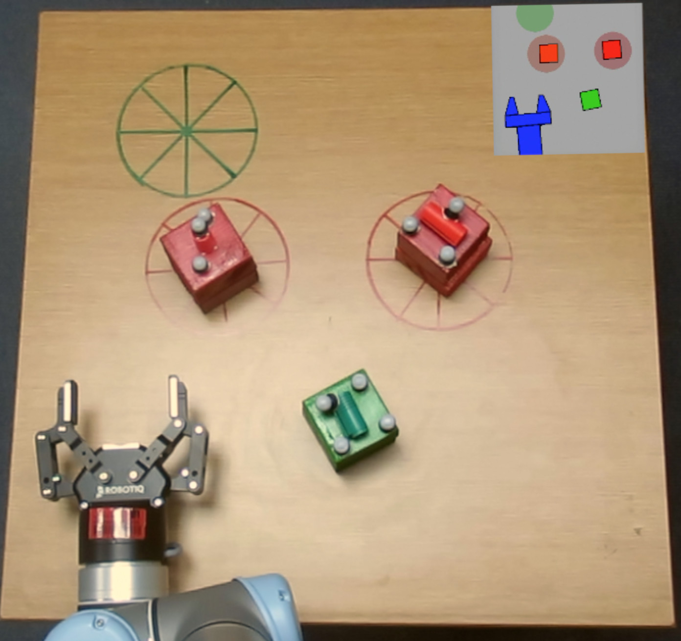
(c)

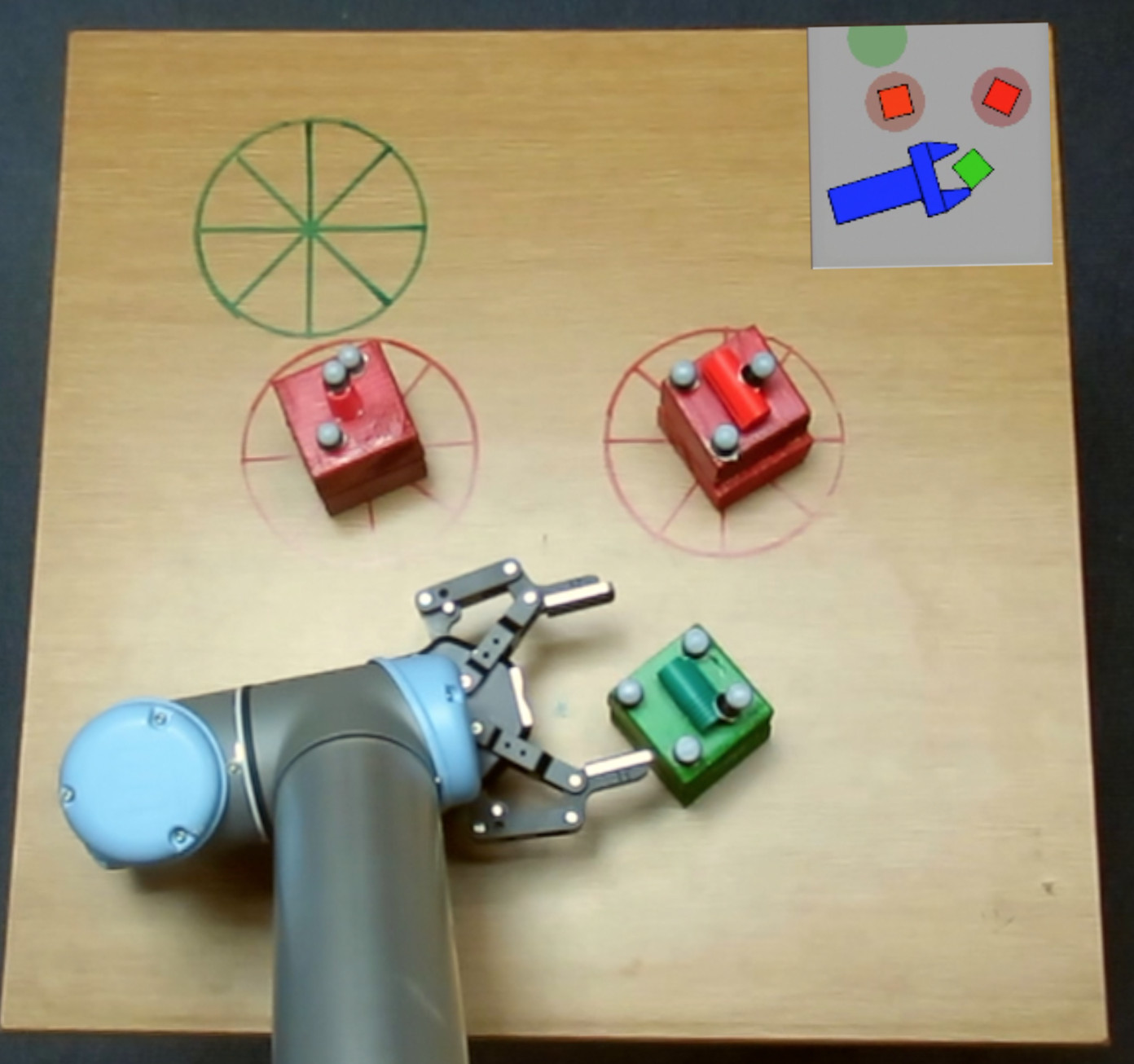
(d)

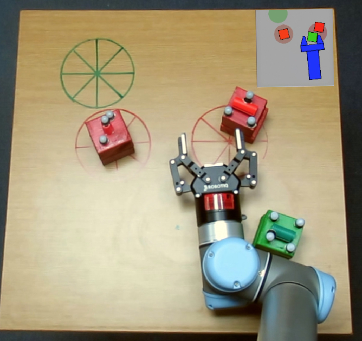
(e)

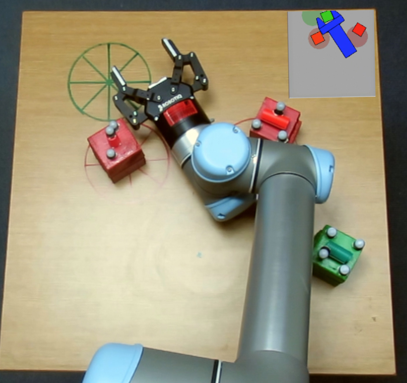
(f)

    Closed-loop

(g)

    RHP execution

(h)

(i)

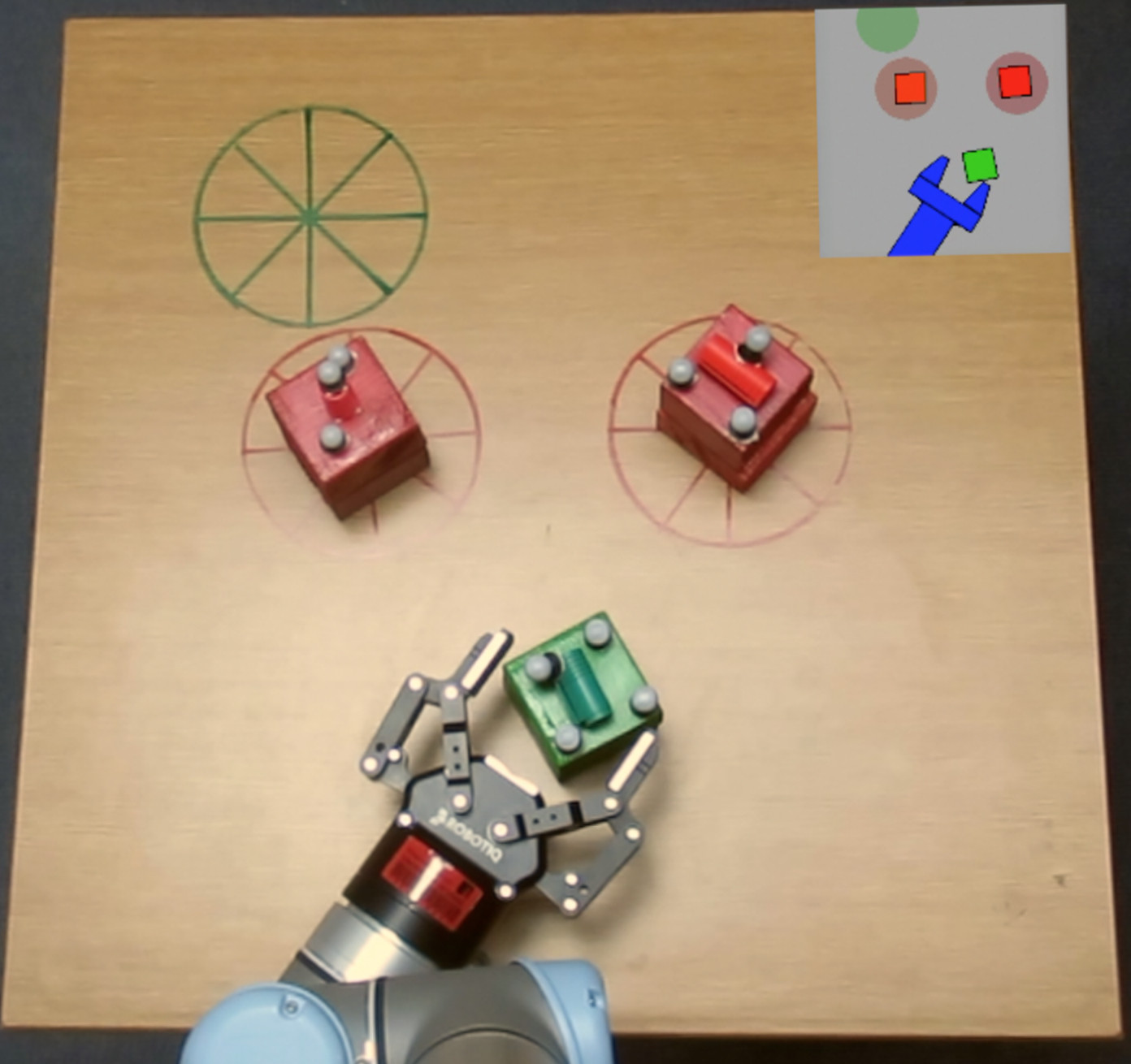
(j)

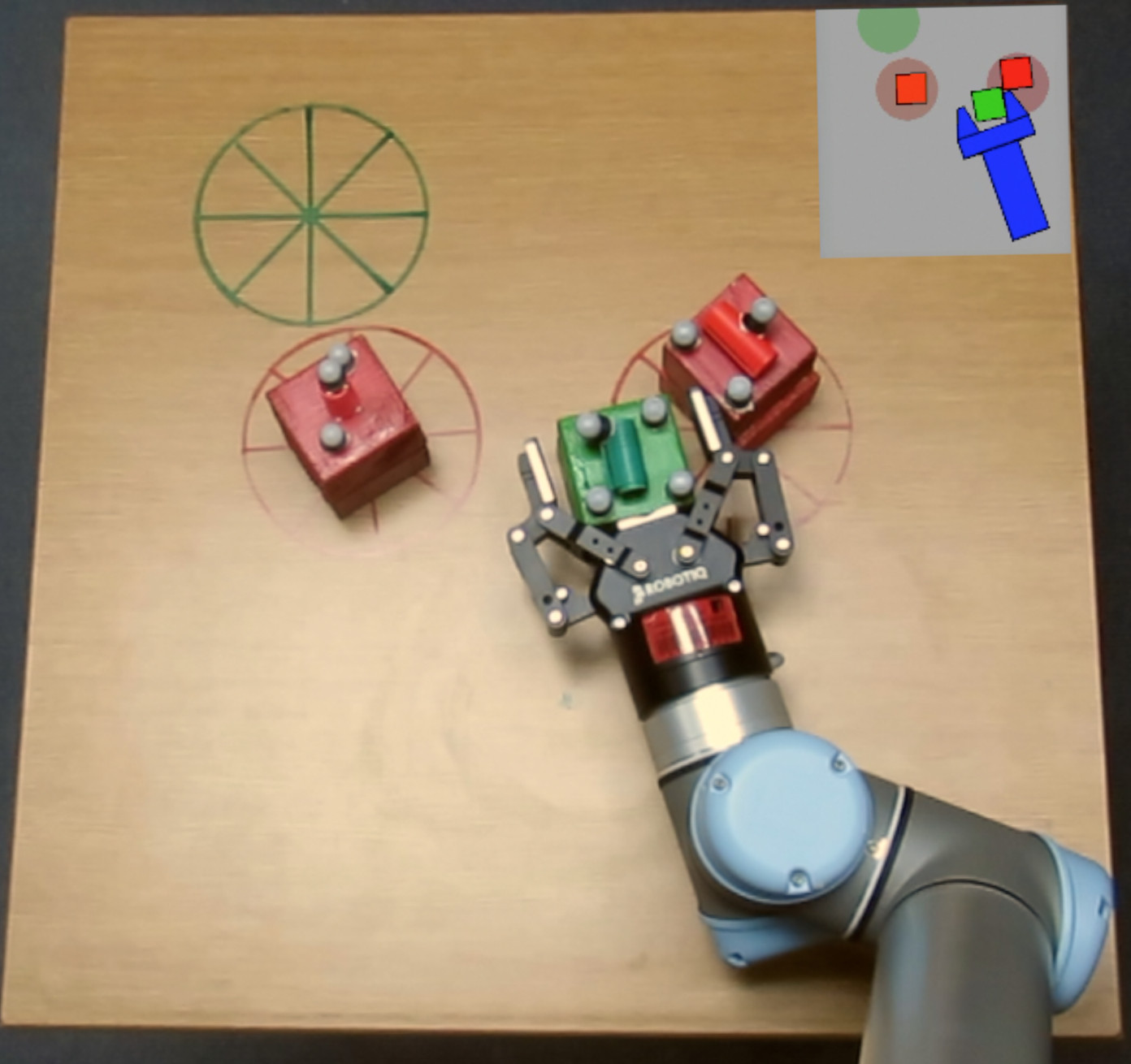
(k)

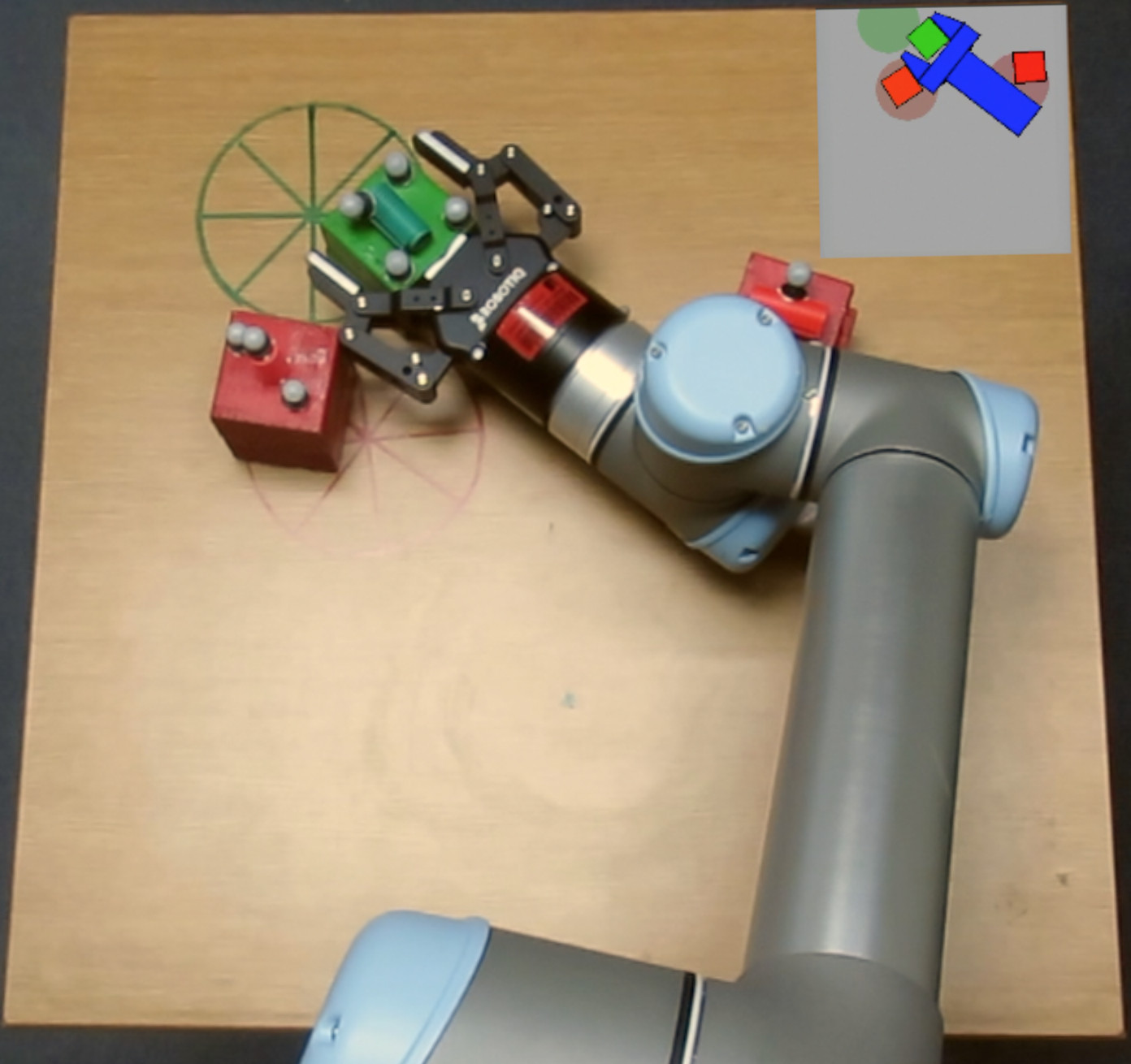
(l)

Figure 1: Top: robot failing to push the green box to the goal region by following a precomputed plan using kino-dynamic planning. Bottom: robot successfully executing the task using closed-loop RHP execution.

The top row of Fig. 1 shows the execution of an open-loop trajectory generated by a sampling-based planner, while the bottom row presents an execution of our system. The overlaid animated figures (on the top-right corner of the images) show the planner’s prediction of how the objects should move during interaction. When planned trajectories are executed open-loop, the real motion of the objects can differ significantly from the motion predicted by the planner. For this reason, in the shown example, the open-loop controller fails to accomplish the task.

A solution to this problem is to interleave planning and execution. In this approach, a sequence of actions is planned, but only the first action in this sequence is executed. Then, the current state is updated by observing the environment, after which another sequence of actions is planned, and the routine is repeated. This idea is commonly used in domains that involve uncertainty, and underlies many similar methods with different names, among which: rolling horizon planning, receding horizon control, and model predictive control. We show an execution of such a controller in the bottom row of Fig. 1. Even if objects move differently than predicted, the controller has the opportunity to correct for it.

One possible approach to generating such a receding horizon planner (RHP) would be to run one of the aforementioned planners at every step of the execution, to generate the new sequence of actions. The computation time these planners require, however, is prohibitively high, typically taking from tens of seconds to minutes for one plan [7, 4, 5, 6, 2, 8, 9]. In contrast, we are interested in real-time execution, which requires a planner that can quickly suggest an action for the current state of the world.

To generate plans quickly, we propose to run RHP with a short horizon into the future, and take advantage of an appropriate cost-to-go function as a proxy for the value of the states beyond the horizon. This value of a state must estimate how costly (or rewarding, depending on the formulation) it would be to reach the goal from that state. In domains where multiple physics-based object-to-object contact is possible, defining this function is a challenge on its own.

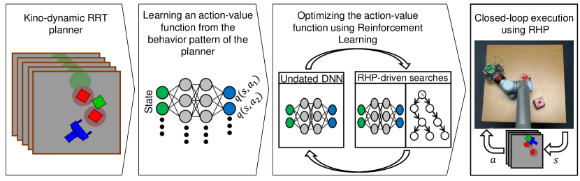
Figure 2: Overview of the proposed approach.

In this paper, we propose to use data-driven techniques to learn such a value function, so that we can then use it as a heuristic within a receding horizon planner. In order to do this, in simulation, we generate many planning instances, and we solve them using an existing sampling-based planner (a kino-dynamic RRT planner [4]). We then use the sequences of states and actions in these plans to train a Deep Neural Network (DNN), to predict the value of a state-action pair, that is, the expected reward for reaching the goal starting from that state and using that action.

The value function learned at this stage leads to an acceptable controller when used as a heuristic, but as we show in our results, it can be further improved. Our insight is that the DNN, trained only by the sampling-based planner, encodes the value of a state under the planned trajectory, which differs from what the robot will actually execute when controlled by RHP. Therefore, we use a reinforcement learning (RL) algorithm to gradually update the value function to better estimate the actual optimal value of the manipulation task.

Our key contribution is in showing that such an approach gives promising results in the domain of physics-based manipulation in clutter: the robot is able to perform fast closed-loop re-planning to deal with the inherent uncertainty in this domain, which challenges existing planners. We show that a heuristic value function can be learned using sampling-based planners and deep learning. Furthermore, we show that it can be improved using reinforcement learning. We perform simulated and real-world experiments to evaluate the performance of our planner.

II Related Work

The planners discussed so far [4, 5, 6, 2] adopt an approach of motion planning followed by open-loop execution to solve the problem of manipulation in clutter. In particular, Haustein et al. [4] adopts sampling-based planning to solve this problem. They propose reducing the search space of kinodynamic Rapidly exploring Random Trees (RRT) by planning over statically stable environment states while allowing for physical interaction in-between these states. In this paper, we use a similar kinodynamic RRT planner to generate plans to different manipulation problem instances. There are planners which also take uncertainty into account before the generation of the motion trajectory [2, 10, 8, 9], but these planners typically rely on uncertainty reducing actions which generate a conservative sequence of actions, limiting the robot from using the complete dynamics of the domain.

In this paper, however, we are mainly interested in real-time planning which can be used in a closed-loop system to respond dynamically to changes during execution. Kloss et al. [11] present a learning approach for planar pushing tasks in closed-loop form. They train a neural network, which takes the visual state of the environment as input, and feeds the appropriate physical properties extracted from the scene to an analytical model of the task. Hogan and Rodriguez [12] apply a feedback control scheme that can alternate between different interaction modes to control a tool pushing a slider on a planar surface. To avoid learning a behavior that exploits the idiosyncrasies of the physics model in the simulation environment, Peng et al. [13] propose randomizing the physics parameters in the simulation environment during the learning phase for a pushing task. These approaches have proven capable in real world manipulation. However, they focus on manipulating a single object whereas we are interested in multi-object interaction present in cluttered spaces. Laskey et al. [14] tackles this problem by relying on a expert human demonstrator and a DNN to control 2-DOF of a robot arm to reach a target object on a cluttered surface.

The idea of learning a heuristic for control and planning has been applied in domain other than manipulation in clutter. Negenborn et al. [15] propose a framework for learning based model predictive control for general Markov Decision Process. Similarly, Zhong et al. [16] look at the problem of value function approximation for automatically shortening the horizon in model predictive control for dynamic tasks like inverted pendulum and acrobot. These approaches do not take into account challenges typical to clutter manipulation tasks, such as inaccuracy of the physics model, and computation constraints imposed by the physics engine. Conceptually, the work of Anthony et al. [17] is reminiscent to our work. They use Monte Carlo Tree Search to generate plans leading to the goal. They suggest making the searches more efficient by biasing the search process with a DNN-based value function that is recursively trained on previous iteration of the generated plans. Likewise, Hottung et al. [18] integrate neural networks in a heuristic tree search procedure for accelerating the searches by pruning the tree. Further, Hussein et al. [19] rely on collected demonstrations to pre-train a DNN-based policy. Then, they refine the policy in an active learning fashion where an agent is assumed to have access to the optimal policy when faced with states with low action confidence. Although combining traditional control and theoretic planning such MCTS methods [20, 21] with machine learning offers promising solutions to problems with a sparse reward function [22], they are yet to be proven capable in handling physics based manipulation, where simulating a large number of roll-outs (a common feature of these approaches) at every time step is prohibitively expensive. To the best of our knowledge, this line of thought has not yet been investigated in the context manipulation in clutter. In this paper we examine the problem from a physics based perspective for real world applications.

III Problem Formulation

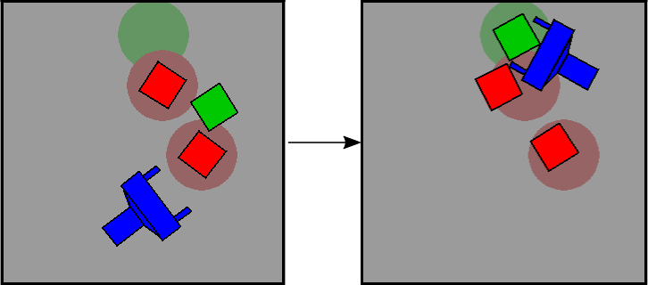
Figure 3: The initial configuration (left) and the final configuration (right) of an example scene.

We target applications where a robot has to reach and manipulate objects in cluttered spaces. For instance, reaching a ketchup bottle in the back of a cluttered refrigerator shelf, or pushing a box item on a warehouse shelf. In these settings, it is also desirable to minimize the disturbance of other objects while manipulating the target object. The robot has to use non-prehensile skills to manipulate movable objects from an initial state to a desired goal state, as illustrated in Fig. 3.

We model the environment as a Markov Decision Process (MDP) represented as a tuple ${M=\langle S,A,T,r,\gamma\rangle}$ where $S$ and $A$ are the sets of states and actions respectively, ${r:S\times S\rightarrow\mathbb{R}}$ is the reward function, ${T:S\times A\rightarrow S}$ is the transition function, and $\gamma$ is the discount factor, such that ${0\leq\gamma\leq 1}$. Since we are interested in modeling planning problems with goal states, our MDP model is episodic, that is there exists at least a (goal) state $s_{g}$ that can never be left ($T(s_{g},a)=s_{g}\;\forall a\in A$) and gives zero reward ($r(s_{g},s_{g})=0$). A behavior for the MDP is represented as a (stochastic) policy $\pi:S\times A\rightarrow[0,1]$, where $\pi(s,a)=P(a|s)$, with $s\in S,a\in A$, that is, the probability of the agent picking action $a$ in state $s$. The value of a state-action pair $\langle s,a\rangle$ under a given policy $\pi$ is the cumulative discounted reward (called the return) achieved from $s$ taking $a$ and following $\pi$ thereafter: $q^{\pi}(s,a)=\sum_{t=0}^{\infty}\gamma^{t}r_{t+1}|_{\pi}$

The state at time $t$ is given by the planar poses of the robot and the $m$ objects $s_{t}=\{\langle x_{\textrm{robot}},y_{\textrm{robot}},\theta_{\textrm{robot}}\rangle,$ $\langle x_{\textrm{obj\_}i},y_{\textrm{obj\_}i},\theta_{\textrm{obj\_}i}\rangle_{i=1}^{m}\}$. While the state space is continuous, we discretize the action space, so that the robot can execute six actions in $A$, four to apply a force in each of the cardinal directions, and two to rotate the end-effector clockwise and counterclockwise in the task space. The transition function $T$ models the physics-based interaction between the robot and the objects, predicting how the objects move in response to robot actions. We avoid hand-crafted reward functions by setting $r(s_{t},s_{t+1})=r_{t+1}=-1$ where $s_{t},s_{t+1}\in S$. This domain-independent reward function encourages the robot to reach the goal ${S_{\textrm{goal}}\subseteq S}$ as fast as possible.

A task instance $\langle s_{init},G\rangle$ for our problem is defined by the initial positions of the robot and objects, $s_{init}$, and a set of circular goal regions for all objects ${G=\langle x_{\textrm{goal\_}i},y_{\textrm{goal\_}i},radius_{\textrm{goal\_}i}\rangle_{i=1}^{m}}$, where $x_{\textrm{goal\_}i}$ and $y_{\textrm{goal\_}i}$ is the centre of the goal region for object $i$ and the $radius_{\textrm{goal\_}i}$ is the radius of this region. Example regions are in Fig. 3. In this paper, for the obstacle objects (red objects in the figure), we place the goal regions (red regions in the figure) on the initial positions of these objects at $s_{0}$. This is how we discourage the planner from disturbing the scene. For the target object (green object) the goal region (green region in the figure) can be anywhere. We also use the same fixed radius for all goal regions. The goal set ${S_{\textrm{goal}}}$ is the set of all the states where all the objects are in their goal regions $G$.

A plan is a sequence of states and actions ${p=\langle s_{0},a_{0},\ldots,s_{L-1},a_{L-1}\rangle}$, where $L$ is the length of the plan, $s_{t+1}=T(s_{t},a_{t})$ with $s_{t},s_{t+1}\in S$, and $T(s_{L-1},a_{L-1})\in S_{g}$, i.e. the final state is a goal state. An optimal plan is one that maximizes the return from the initial state.

Existing planners [2, 4, 5, 6] can generate solutions to this problem (which are usually sub-optimal in the sense of maximizing the return, but can at least find a plan to reach a goal state). However, open-loop execution of these plans in the real world can easily fail, as the predicted motion of the objects differs from the real motion due to uncertainty in physics-based predictions, especially when there are multiple contacts between objects.

In order to take the model uncertainty into account, we propose to interleave planning and execution, where the robot:

1. Plans a sequence of actions from the current state $s_{0}$.

2. Executes the first action, $a_{0}$, in the sequence.

3. Observes the state of the system and update $s_{0}$.

4. Goes to step 1.

The first step in this procedure is usually the most costly one. The planners in the literature addressing the problem of manipulation in clutter are not fast enough (taking anywhere from tens of seconds to minutes [2, 4, 5, 6]) to run as step 1. Therefore, in this paper, we propose to plan for only a short horizon, and not necessarily until the goal. Given such a horizon $h$, we are then interested in maximizing the reward for $h$ steps plus our estimate of how much reward we can get from the state at the horizon:

$$\langle a_{0},\ldots,a_{h-1}\rangle=\operatorname*{arg\,max}_{\langle a_{0},\ldots,a_{h-1}\rangle}\sum_{k=0}^{h-1}\gamma^{k}r_{k+1}+\gamma^{h}\max_{a}q(s_{h},a)$$ (1)

where the action-value function $q(s_{h},a)$ estimates the expected return for reaching the goal from the horizon state $s_{h}$ and choosing the action $a$. In this paper, we call this the Receding horizon planner (RHP) and we use it as the robot control policy.

The horizon can mitigate the inaccuracy of the value function estimate, by ranging from infinity, with the robot planning all the way to the goal, to zero, with the robot acting greedily with the respect to the value function. With an infinite horizon the value function is ignored, while with $h=0$ the behaviour depends entirely on the value function. In the latter case, if the value function is optimal (that is $q(s,a)\geq q^{\pi}(s,a)\;\forall s\in S,a\in A$, for any policy $\pi$), so is the resulting policy. In practice, a short but non-zero horizon takes advantage of both the planner and the value function without relying on either one entirely, and we experiment with several values for $h$.

IV Learning an action-value function from sampling-based planners

We are interested in having an approximation of the action-value function over the entire continuous state-space for any goal. In this section, we present a learning approach to extract an estimate of the action-value function from a collection of planning instances. The learned function approximates the return achieved by the planner from a number of sampled initial states and goal regions.

IV-A Generating example plans

Sampling-based planners treat every new planning instance independently from previously solved instances. Also, they must plan until the goal, which means that they do not offer useful information on the searched areas of the state-state space from which the goal was not reached. However, sampling-based planners provide a probabilistically complete tool to solve complex planning problems in high-dimensional state spaces without necessarily requiring a hand-crafted or domain-dependent heuristic. In particular, Kino-dynamic planners are one family of the sampling-based Rapidly exploring Random Trees planners, specific for solving planning problems that involve dynamic interactions. We implement a state-of-the-art kino-dynamic planner [4] used for solving physics-based manipulation in clutter planning problems. We generate $P$ random problem instances $\langle s_{init}^{p},G^{p}\rangle_{p=1}^{P}$, as described in Sec. III. Then, for each planning instance $p$, we run the kino-dynamic planner to generate a solution of the form $\langle a_{init}^{p},\ldots,a_{L-1}^{p}\rangle$. The state trajectory $\langle s_{init}^{p},\ldots,s_{L-1}^{p}\rangle$ induced by the action sequence of a plan $p$ brings the environment to a goal state $T(s_{L-1}^{p},a_{L-1}^{p})\in S_{g}^{p}$ where each box is placed in its corresponding target region $G^{p}$.

IV-B Learning The Action-Value Function From Observed Trajectories

We use example plans to train a DNN to predict the action-value estimate for a given state-action pair. We represent the action-value function estimate $\hat{q}(s,a;\theta)$, modeled by a DNN with parameters $\theta$. To train the DNN, we use every state-action pair encountered along every example plan. For each example plan, and for every state-action pair in that plan, we compute the update target:

$$q(s_{l}^{p},a_{l}^{p})=\sum_{k=0}^{L-l-1}\gamma^{k}r_{l+k+1}=r(\frac{1-\gamma^{L-l}}{1-\gamma})$$ (2)

where $p$ stands for the index of the plan generated by the kino-dynamic planner and $l$ is the index of the state-action pair in that plan. The second equality takes advantage of the fact that in our formulation all the immediate rewards, denoted as $r$, are the same.

While the DNN trained as above learns to predict the action-values for the actions executed in a state by the kino-dynamic planner, the values predicted by the DNN for actions that have not been used by the planner can be arbitrary. This is because the available example plans offer no information on the actions that the planner did not choose along the traversed states. As a result of function approximation, however, these actions will nonetheless have a value. The value can converge to an arbitrary number, determined by the effect of the target value in the states that the planner did traverse. A possible undesirable effect is that the values of the actions not chosen by the planner can be higher than the chosen one. This can later cause an action that was not favored by the kino-dynamic planner to look more favorable to RHP that uses the action-value function as a heuristic.

In order to avoid this phenomenon, we ground the unchosen actions to a target value that is lower than the target value of the chosen action. In literature [23, 24], the difference between the value of a desired action and the other actions is referred to as the value margin

We propose a definition of the value margin driven by the observation that, in the domain of pushing tasks, a mistake is in most cases not irreparable, but can be overcome through a number of $k$ additional actions. Hence, we use for the action-value of the unchosen actions the following update target:

$$q(s_{l}^{p},a_{u}^{p})=\begin{cases}r(\frac{1-\gamma^{L-l+k}}{1-\gamma}),\,&\text{if}\ \hat{q}(s_{l}^{p},a_{u}^{p};\theta)\geq q(s_{l}^{p},a_{l}^{p})\\ \hat{q}(s_{l}^{p},a_{u}^{p};\theta),\,&\text{otherwise}\end{cases}$$ (3)

where $a_{u}\in A\setminus\{a_{l}\}$ is an unchosen action. This imposes that the unchosen actions, which would otherwise have a higher value than the chosen one, have a value equivalent to being $k$ steps further away from the goal than the chosen action. If, on the other hand, the value that the approximator converges to does not favor an unchosen action then we leave it unchanged (as estimated by the network). Lastly, we add an $L_{2}$ regularization term to the target function of Eq. 2 and 3, to avoid over-fitting on the available plans. Once the training converges, we can use the action-value function to derive RHP policy for the robot, as described in Sec. III.

We experimented with DNNs of different sizes and expressive power, but none could reliably represent the behavior of the planner over a large number of task instances. We demonstrate experimentally that executing a greedy policy directly on the output of the network leads to a success rate much lower than using the action-value function as heuristic for RHP policy, i.e. using the action-value function only after a few lookahead steps. Nonetheless, we show in the next section that the information compiled in the action-value function can be further optimized to play a valuable role when used as a heuristic to drive RHP.

V Heuristic-Guided Deep Reinforcement Learning

The performance of action-value based RHP is bounded by the quality of its heuristic. So far, the knowledge encapsulated in the action-value function has two shortcomings: first, the plans generated by the kino-dynamic planner are, in general, sub-optimal; and second, information is lost in the approximation by the DNN, with consequent performance degradation with respect to the kino-dynamic planner. Furthermore, the action-value function estimates the return based on the average behavior of the kino-dynamic planner. However, the RHP policy, that is actually controlling the robot, can differ from the behavior of the kino-dynamic planner. To overcome these problems, we use reinforcement learning to 1) improve the action-value function to better estimate the optimal one and to 2) ground the unexperienced state-space transitions to their actual values.

We implement the Deep Q-Learning (DQN) algorithm [25]. We initialize the DNN to the trained DNN from the previous section. Further, We formulate an RL policy, that we call $\epsilon$-RHP, which selects a random action with probability $\epsilon$ and with probability $1-\epsilon$ the policy queries RHP for an action. We found that focusing the search towards the goal by augmenting the RL policy with RHP, reduces the chances of the action-value function from diverging which is common problem in RL when used in conjunction with a DNN as a function approximator.

Throughout the RL training process, the robot stores the newly collected transition samples in a finite buffer $D^{replay}$, initialized with transition samples from the previously solved task instances, and gradually replacing old samples. At every action step, the DNN parameters are updated by minimizing a loss function on a batch of random transition samples from $D^{replay}$. The loss function is the squared prediction error over the $M$ samples in a batch $B=\{\langle s_{i},a_{i},r_{i},s^{\prime}_{i}\rangle_{i}\}$ where $s^{\prime}_{i}$ is the state following $s_{i}$ in sample $i$:

$$L_{\theta}(B)=\sum_{i=1}^{M}(r_{i}+\gamma\max_{a^{\prime}_{i}}\hat{q}(s^{\prime}_{i},a^{\prime}_{i};\theta)-\hat{q}(s_{i},a_{i};\theta))^{2}$$ (4)

We also add an $L_{2}$ regularization loss on the network parameters.

The benefit of $D^{replay}$ is twofold. It is using the collected experience more effectively to counteract the high correlation in the on-line incoming samples, which is also known as experience replay. Second, it leads to a smooth change in the action-value function, and consequently in the robot behavior, as it shifts from estimating the cost of following the kino-dynamic planner to estimating the optimal action-value function.

VI Searching the action-space up to the horizon

We use the learned action-value function $\hat{q}(s,a;\theta)$ as heuristic to RHP, i.e. we use it as an approximation in Eq. 1 in-place of the unknown optimal action-value function at $s_{h}$.

The only remaining problem is searching the action-space up to the horizon, i.e. the maximization over the $h$ actions in Eq. 1. One naïve way to do this is to explore all possible action sequences up to the horizon $h$. However, an exhaustive search would scale badly with the horizon depth $h$ and the size of the action set $A$, $\mathcal{O}(|A|^{h})$.

Instead, we bias the search towards promising actions. We implement RHP, such that it simulates $n$ trajectories, which we call roll-outs, of horizon $h$ each. Each of the $n$ roll-outs is started from the current state $s_{0}$. At every step $t$ in a roll-out, RHP samples an action using the soft-max of the action-value function:

$$P(a|s_{t})=\frac{exp(\hat{q}(s_{t},a;\theta)/\tau)}{\Sigma_{a_{i}\in A}exp(\hat{q}(s_{t},a_{i};\theta)/\tau)}$$ (5)

where $\tau$ is the temperature parameter. This would favor exploring actions whose value learned in the previous section is the highest. The return of a roll-out is computed as an $h$-step return, where the first $h$ rewards are generated by the model, and the action-value function acts as a proxy for the rewards beyond the horizon:

$$R_{0:h}=r_{1}+\gamma r_{2}+\ldots+\gamma^{h-1}r_{h}+\gamma^{h}\hat{q}(s_{h},a_{h};\theta).$$

RHP then executes the first action in the roll-out that obtains the highest return. This procedure reduces the number of simulated actions per RHP query to $n\times h$. The action-value function, therefore, plays two roles: to inform the search through the soft-max sampling, and as a proxy for the rewards that are not sampled from the model.

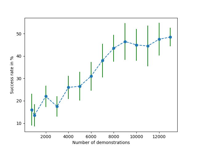
Figure 4: Performance of the greedy policy induced by the action-value function trained over a different number plans.

VII Evaluation

The manipulation scenario follows the same model introduced in Sec. III. As shown in Fig. 3, the environment consists of the end-effector of the robot arm shown in blue and 3 movable square boxes of side $6\ cm$ on a planar surface shown in red and green. The robot has to push one of the boxes into a desired target region of radius $6\ cm$, while having the rest of the objects placed by the end of the task as close as possible to their initial pose. The target regions are depicted by light colored circles corresponding to their designated boxes.

We evaluate the proposed approach in three experiment sets:

• First, we measure the effect of the number of plans (that is, plans generated by the kino-dynamic planner) on the quality of the action-value function. We show that after a certain number of plans from the planner, the performance of the induced policy hits a plateau.

• Second, we compare the performance of our trained planner to different base line approaches.

• Lastly, we demonstrate some example plans on a real world implementation.

In our simulation experiments, we modeled the world in the Box2D physics simulator [26]. The robot motion is generated by applying momentary forces to its end-effector, and waiting until the robot and objects came to a stop due to frictional damping forces. With this force, we observed that each translational action moved the hand for a distance of around $5\ cm$, and each rotational action moved the hand for about $30^{o}$. The kino-dynamic planner typically needed 20-30 actions to reach the goal in our experiments in a wide variety of task instances. Therefore, we set 40 actions as the limit before we stopped our policy. At the end of a run, if any the boxes was out of its corresponding target region, then we considered that run a failure. Otherwise, we considered it a success.

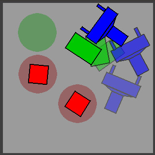
(a) Kinodynamic Planner

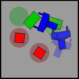
(b) RHP

Figure 5: Evaluation at execution time with shape uncertainty.

VII-A The effect of the dataset size on performance

We generated multiple task instances by randomly sampling non-colliding initial object poses and also randomly sampling a target region for the green box. We then run the kino-dynamic planner to generate a plan for each the task instances. We used the TensorFlow [27] library to build and train a feed-forward DNN model consisting of 5 fully connected layers. The first 4 layers have 330, 180, 80, and 64 neurons, respectively, with ReLU activation function. The output layer consists of 6 neurons, one per action, with linear activation functions. The DNN is trained following the procedure described in Sec. IV-B with the value margin parametrized by $k=4$.

To test the action-value function encoded by the network, we generated 500 random task instances, and run a greedy policy on them, that is executing the action with the highest value estimate. The horizontal axis in Fig. 4 shows the number of plans $P$ generated by the kino-dynamic planner, and the vertical axis shows the success rate of the policy trained with that many plans. We split the 500 task instances into 25 batches of 20, and the figure plots the average success rate and the confidence interval over these batches.

As expected, the graph shows an increasing trend w. r. t. the number of available plans. After reaching a $P$ of 9000 plans, we see that it starts to plateau before it hits $50\%$ success rate. This demonstrates that the DNN alone could not encode, across all instances, a behavior as good as the planner which achieves a success rate of $98\%$ as shown in the first cell of Table I.

    Open-loop

(a)

    Kino-dynamic planner

(b)

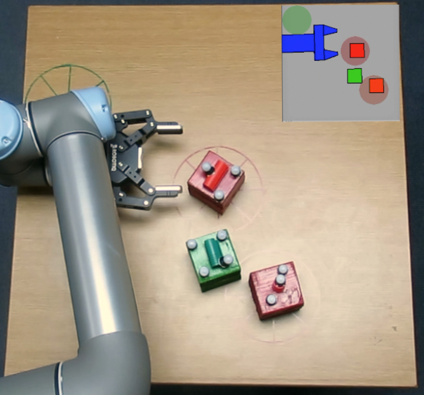
(c)

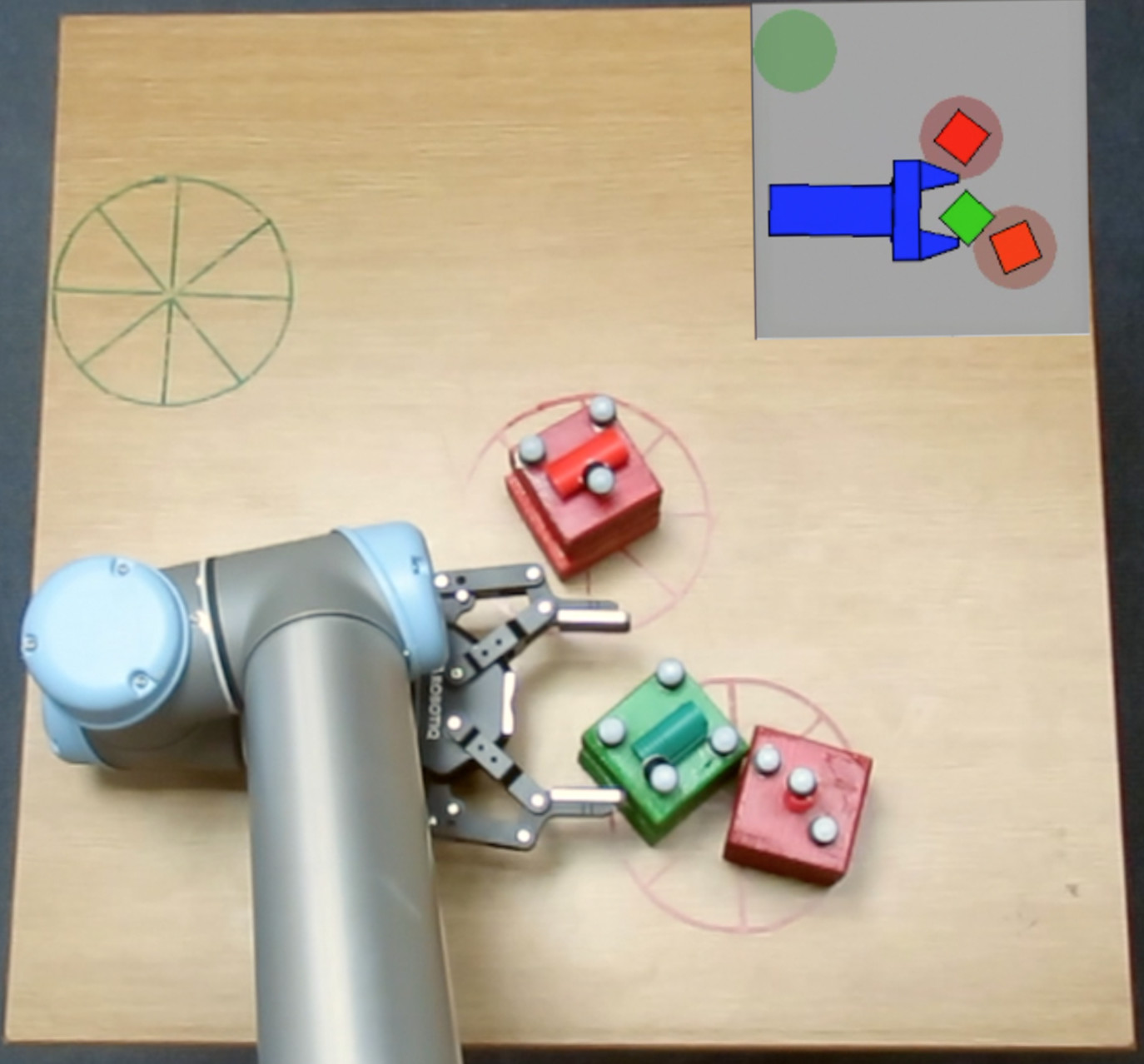
(d)

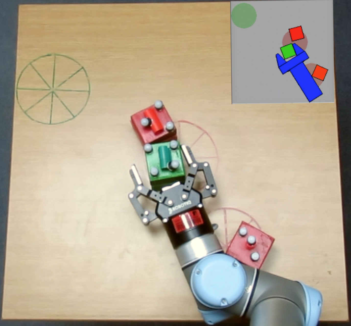
(e)

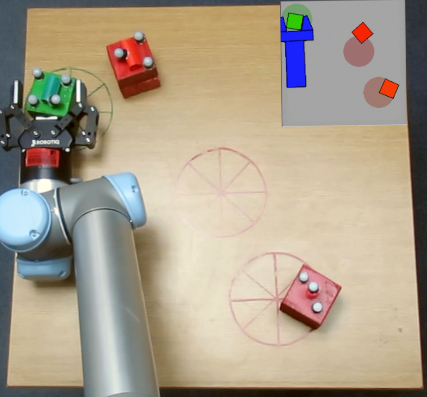
(f)

    Closed-loop

(g)

    RHP execution

(h)

(i)

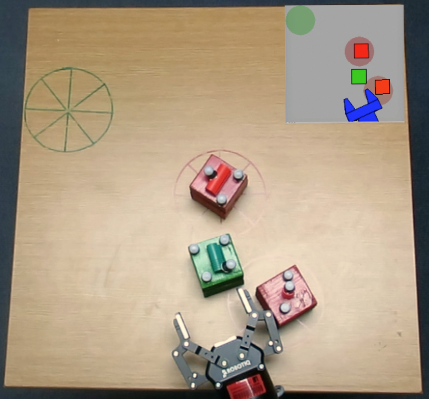
(j)

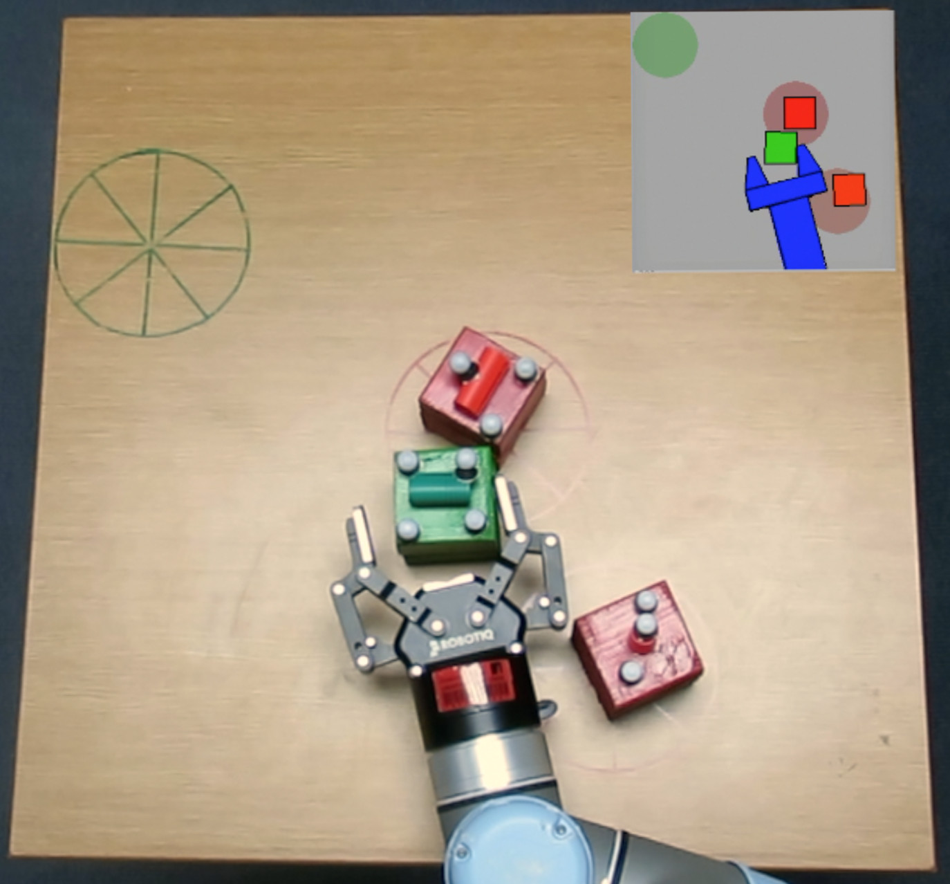
(k)

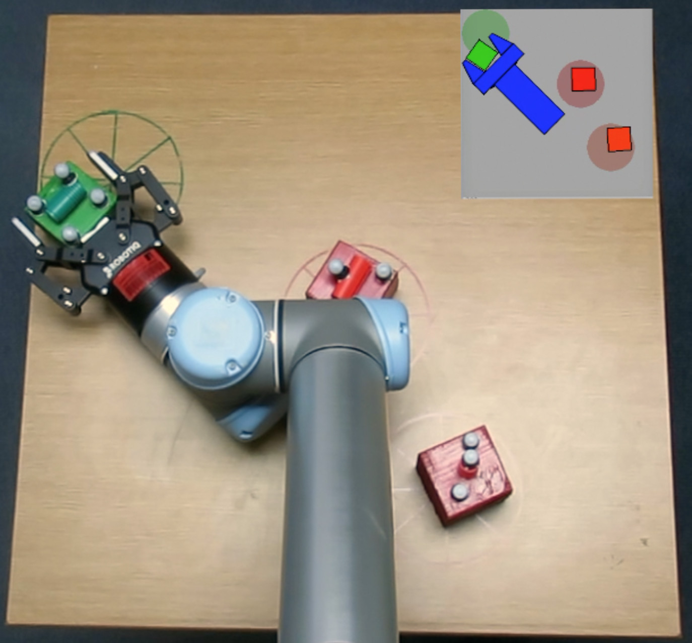
(l)

Figure 6: Top: robot failing to keep the red box close to its initial position by following a precomputed plan using kino-dynamic planning. Bottom: robot successfully executing the task goal using RHP-66.

VII-B Performance evaluation

TABLE I: The performance results of the different policies and the planner

			Planner		Kino-dynamic RHP				Kino-dynamic RHP + RHP-guided RL
			KDP		GP	RHP-33	RHP-66		GP	RHP-33	RHP-66
No uncert.	suc. rate [%]		98.0 $\pm$ 2.0		48.0 $\pm$ 0.0	78.0 $\pm$ 1.9	88.0 $\pm$ 1.9		51.5 $\pm$ 5.6	88.8 $\pm$ 1.3	94.4 $\pm$ 1.6
	Avg. exec. time [s]		49.4 $\pm$ 14.9		0.7 $\pm$ 0.0	5.8 $\pm$ 0.2	17.7 $\pm$ 2.0		0.6 $\pm$ 0.1	7.9 $\pm$ 0.2	21.2 $\pm$ 1.6
Low uncert.	suc. rate [%]		24.5 $\pm$ 17.3		48.2 $\pm$ 7.7	77.2 $\pm$ 4.4	86.2 $\pm$ 3.5		48.6 $\pm$ 6.7	88.2 $\pm$ 2.8	94.0 $\pm$ 2.5
	Avg. exec. time [s]		41.1 $\pm$ 11.7		0.7 $\pm$ 0.1	6.4 $\pm$ 0.5	18.6 $\pm$ 1.6		0.6 $\pm$ 0.0	8.0 $\pm$ 1.3	22.7 $\pm$ 5.6
Med. uncert.	suc. rate[%]		28.5 $\pm$ 25.3		42.2 $\pm$ 12.4	73.4 $\pm$ 4.9	85.8 $\pm$ 8.7		47.3 $\pm$ 9.1	88.0 $\pm$ 2.4	91.2 $\pm$ 4.6
	Avg. exec. time [s]		42.5 $\pm$ 9.0		0.6 $\pm$ 0.1	7.3 $\pm$ 0.1	19.7 $\pm$ 3.5		0.6 $\pm$ 0.1	8.1 $\pm$ 0.6	18.4 $\pm$ 5.2
High uncert.	suc. rate[%]		15.7 $\pm$ 15.1		44.7 $\pm$ 29.9	71.5 $\pm$ 7.2	82.8 $\pm$ 8.1		45.6 $\pm$ 10.4	87.3 $\pm$ 5.1	90.1 $\pm$ 2.8
	Avg. exec. time [s]		37.6 $\pm$ 8.9		0.7 $\pm$ 0.1	7.1 $\pm$ 0.8	14.5 $\pm$ 2.3		0.7 $\pm$ 0.2	8.5 $\pm$ 2.7	17.3 $\pm$ 1.6

Next, the network that encoded the best action-value function as measured by the performance in the first round of experiments is further trained with RHP-guided RL where each RHP query runs $n=6$ roll-outs of $h=6$ horizon depth each. To evaluate the effectiveness of every step in our approach, we compare two groups of RHP policies:

• In the first group, the action-value function (that is, the DNN) is learned solely from the plans over the kino-dynamic planner. We call this kino-dynamic RHP in Table I.

• In the second group, the action-value function is further updated with the RHP-guided RL. We call this kino-dynamic RHP + RHP-guided RL in Table I.

We evaluated each of these groups by using the trained action-value function in three different ways: greedy policy (GP), RHP with $n=3,\ h=3$ (RHP-33), and RHP with $n=6,\ h=6$ (RHP-66). We also include the open-loop execution based on the kino-dynamic planner (KDP) as a base-line.

    Open-loop

(a)

    Kino-dynamic planner

(b)

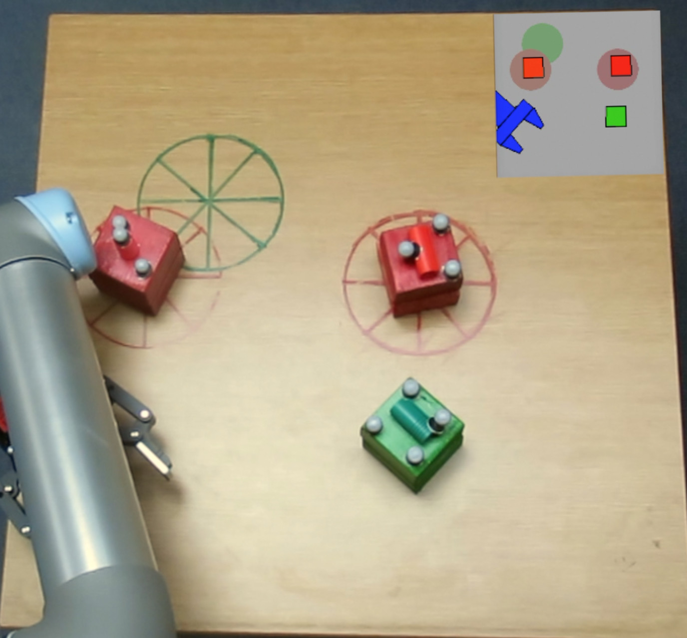
(c)

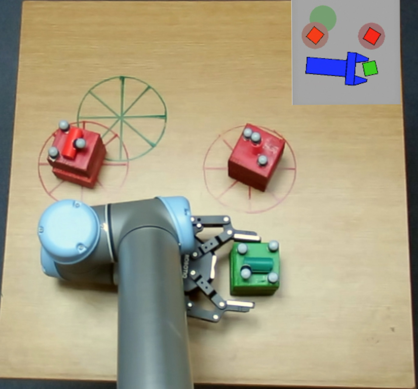
(d)

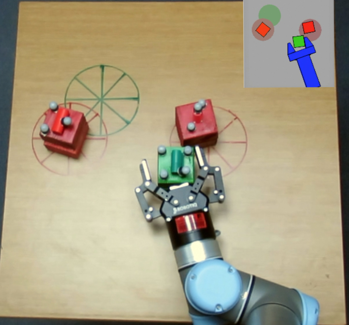
(e)

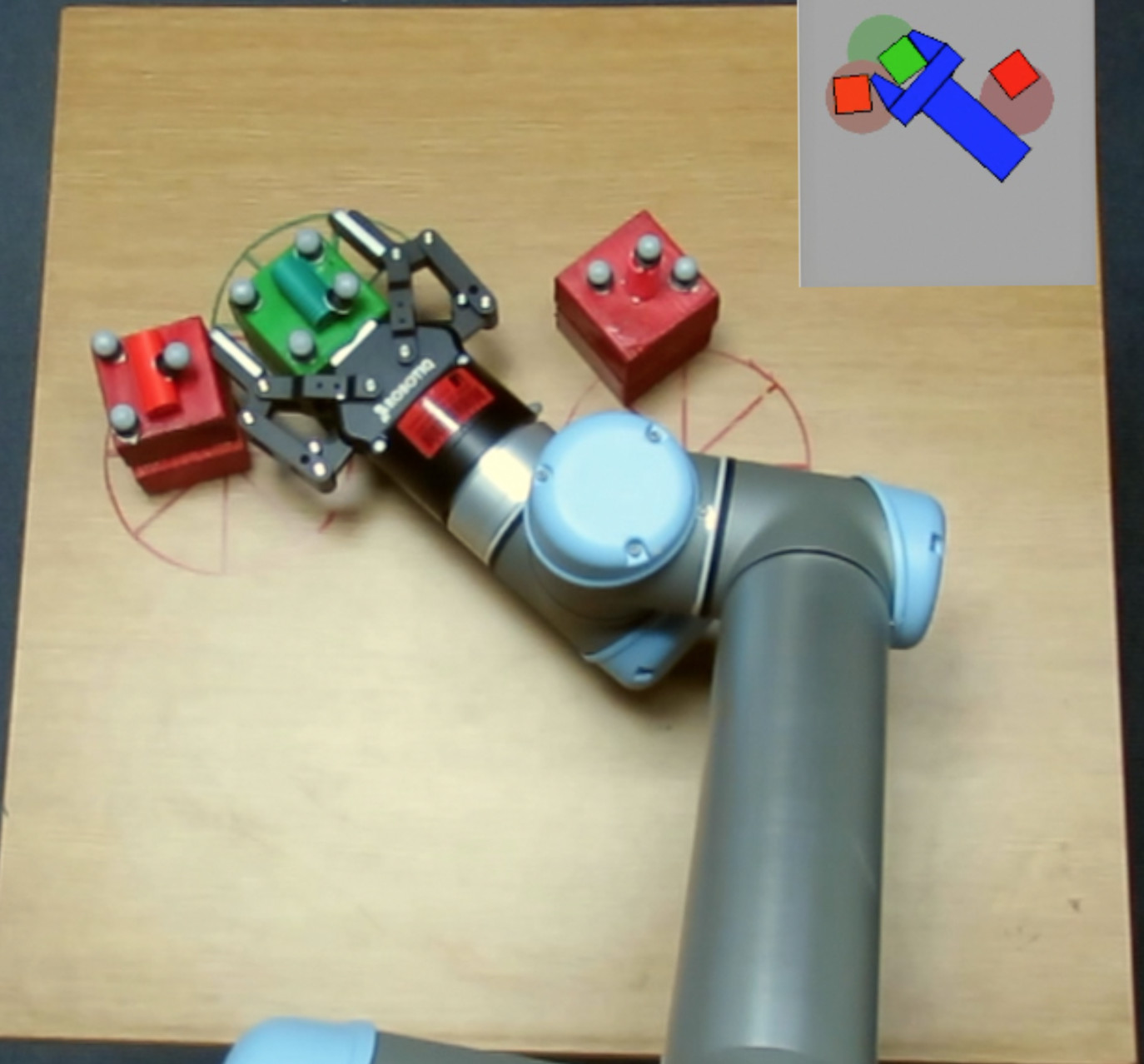
(f)

    Closed-loop

(g)

    RHP execution

(h)

(i)

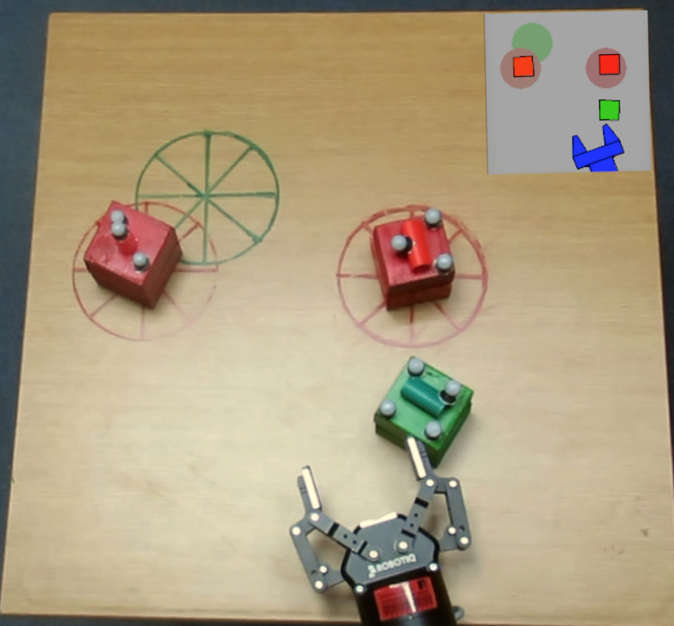
(j)

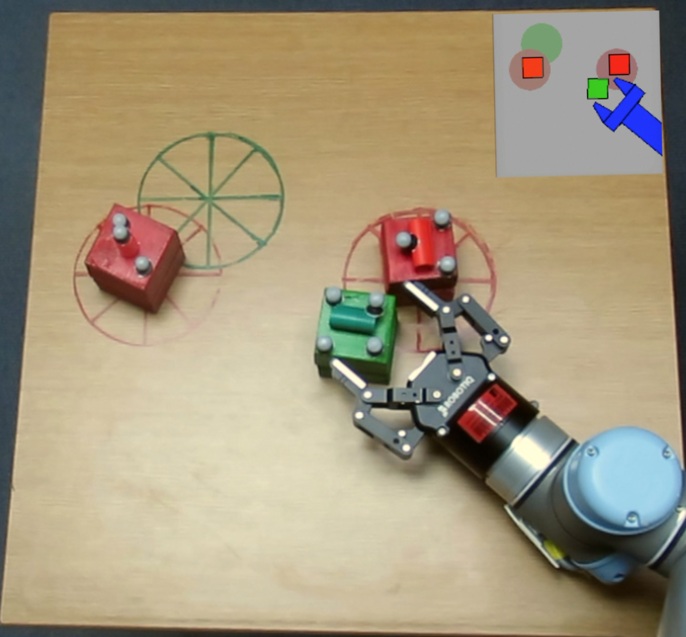
(k)

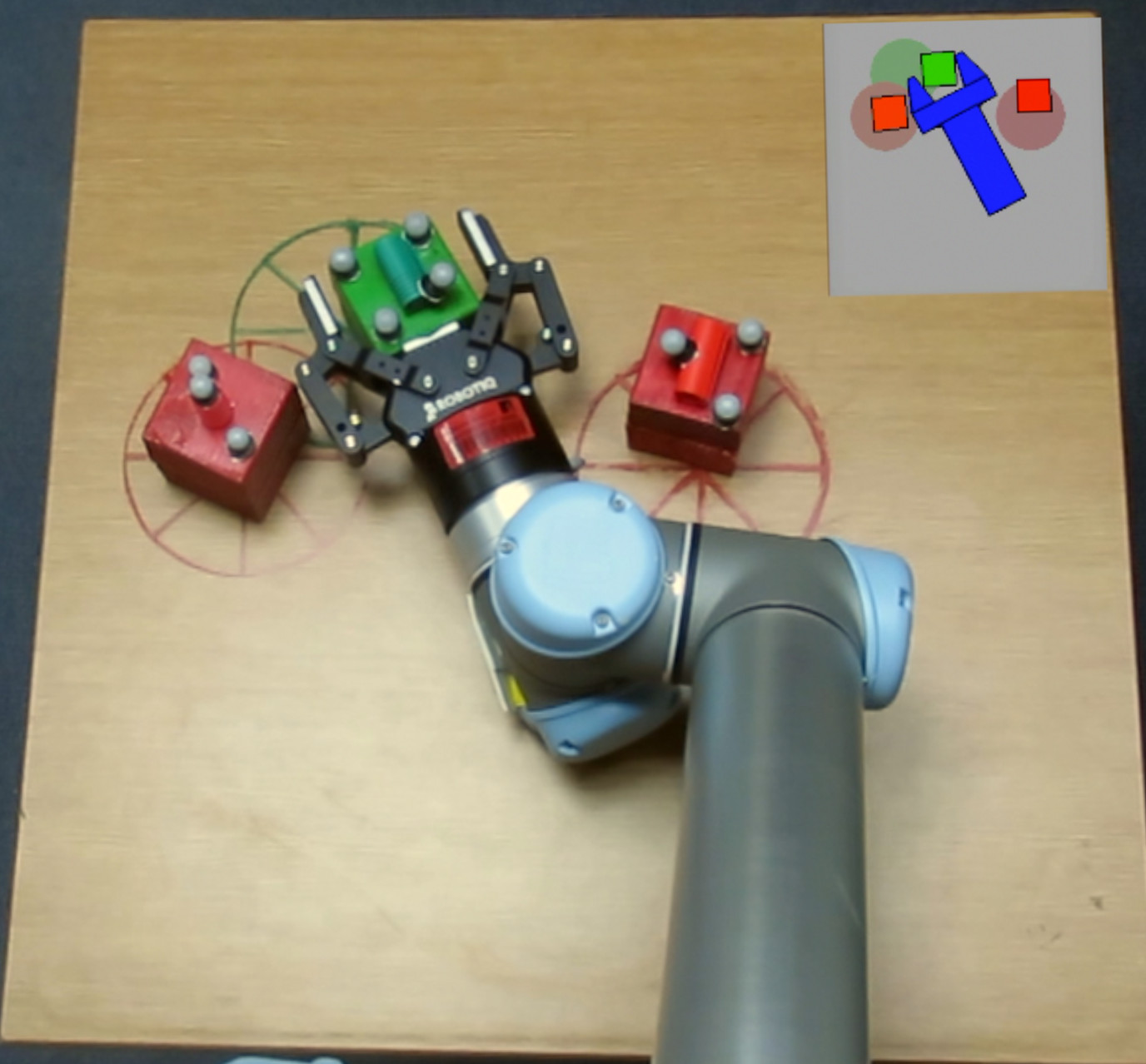
(l)

Figure 7: Top: robot successfully executing the task goal by following precomputed plan using kino-dynamic planning. Bottom: robot successfully executing the task goal using RHP-66.

When we evaluated a certain policy, we injected different levels of uncertainty in the physics model as a way of gaging how a policy copes with dynamics that are different then the one it was trained on. The performance under such artificial uncertainty is a way of estimating the robustness of each policy, and approximating how a policy would perform under real world uncertainty. The rows in Table I correspond to these uncertainty levels.

To inject uncertainty into the execution, we considered physics parameters: shape, friction, and density of the boxes. During evaluation, the uncertainty is sampled from a Gaussian distribution centered around the value of the parameters used in the training (and planning in the kino-dynamic planner case).

In each cell, Table I shows the success rate and the average computation time per successful execution. The latter includes planning time, whether kino-dynamic planning or RHP, and the time required to compute the physical interaction using Box2D. Also, a computation time limit of 2 minutes is imposed on all trials. The results presented are averaged over 10 trials on the 500 random task instances. We note that the experiments are conducted on an Intel Xeon E5-2665 computer equipped with NVIDIA Quadro K4000 GPU card.

The kino-dynamic planner case with no uncertainty shows a high success rate. The few cases where it failed are due to the imposed time limit. Nevertheless, the decreasing performance with uncertainty and the relatively high computation time confirms the limitation of using open-loop planning in execution. The left image in Fig. 5 shows how a plan can fail during execution when the environment is slightly different than expected. The green box was expected to slide inside the robot hand, however because of mismatched dimension, that is, the box has a rectangular shape instead of the square shape used for planning, the box slides outside of the arm trajectory. In general, this indicates that this type of planning is favorable when a high-fidelity model and high-processing power are available.

We also notice that when RHP is engaged there is a notable increase in performance. The longer the horizon and number of roll-outs the higher is the success rate and the more robust it is against uncertainty. The performance increase comes at a cost of an increased computation time. However, it is still within reasonable limits for near real-time manipulation. In contrast to using an open-loop control scheme, the right image in Fig. 5 illustrates how the robot can adapt to unexpected behaviors.

Looking at the overall performance between the two groups of policies, we see that further optimizing the action-value function with RHP-guided RL contributed to a higher success rate and robustness to uncertainty. Particularly, RHP-66 outperformed all of the others w. r. t. the success rate. We used this policy successfully to command a robot in the real world.

VII-C Real robot execution

We performed experiments on a UR5 robot. We created the three task instances shown in Figures 1, 6, and 7. In each task, we tested the trained RHP-66 policy (bottom row in figures) and compared it to the open-loop execution of the kino-dynamic planner (top row). During the execution of RHP, closed-loop feedback on object poses was supplied using an OptiTrack system for RHP to run the roll-outs on the model. As expected, the reactive capability of RHP made its reaction robust to the dynamics of the real world, and succeed in these three tasks. In two out of three tasks, the open-loop execution failed. A video of these experiments is available on https://youtu.be/xwa0fTTuQ1g.

VIII Conclusions

This paper described a receding horizon planning (RHP) approach for closed-loop planning to solve physics-based manipulation in clutter problems in near real-time. We demonstrated how a suitable action-value function for RHP can be learned from a sampling-based planner, and how further improving the action-value function with RL contributes to the system being both faster, and more robust, than the open-loop planner it builds on. Our approach does not require engineering domain-dependent heuristics or manual reward shaping.

These findings motivate us to further develop our research on real-time dynamic manipulation. We are currently extending this work to admit visual input for the state representation. This will allow the robot to seamlessly adapt to a changing number of objects in the scene. We are also committed to augmenting the robot manipulation skills with other manipulation primitives such as grasping, leveraging, and rolling.

References

- [1] D. Leidner, W. Bejjani, A. Albu-Schäffer, and M. Beetz, “Robotic agents representing, reasoning, and executing wiping tasks for daily household chores,” in Proceedings of the 2016 International Conference on Autonomous Agents & Multiagent Systems. International Foundation for Autonomous Agents and Multiagent Systems, 2016, pp. 1006–1014.
- [2] M. Dogar, K. Hsiao, M. Ciocarlie, and S. Srinivasa, “Physics-based grasp planning through clutter,” in Robotics: Science and Systems, 2012.
- [3] C. Hernandez, M. Bharatheesha, W. Ko, H. Gaiser, J. Tan, K. van Deurzen, M. de Vries, B. Van Mil, J. van Egmond, R. Burger, et al., “Team delft’s robot winner of the amazon picking challenge 2016,” in Robot World Cup. Springer, 2016, pp. 613–624.
- [4] J. A. Haustein, J. King, S. S. Srinivasa, and T. Asfour, “Kinodynamic randomized rearrangement planning via dynamic transitions between statically stable states,” in Robotics and Automation (ICRA), 2015 IEEE International Conference on. IEEE, 2015, pp. 3075–3082.
- [5] N. Kitaev, I. Mordatch, S. Patil, and P. Abbeel, “Physics-based trajectory optimization for grasping in cluttered environments,” in Robotics and Automation (ICRA), 2015 IEEE International Conference on. IEEE, 2015, pp. 3102–3109.
- [6] J. E. King, J. A. Haustein, S. S. Srinivasa, and T. Asfour, “Nonprehensile whole arm rearrangement planning on physics manifolds,” in Robotics and Automation (ICRA), 2015 IEEE International Conference on. IEEE, 2015, pp. 2508–2515.
- [7] M. R. Dogar and S. S. Srinivasa, “A planning framework for non-prehensile manipulation under clutter and uncertainty,” Autonomous Robots, vol. 33, no. 3, pp. 217–236, 2012.
- [8] A. M. Johnson, J. King, and S. Srinivasa, “Convergent planning,” vol. 1, no. 2, pp. 1044–1051, July 2016.
- [9] Muhayyuddin, M. Moll, L. Kavraki, and J. Rosell, “Randomized Physics-based Motion Planning for Grasping in Cluttered and Uncertain Environments,” ArXiv e-prints, Nov. 2017.
- [10] M. C. Koval, J. E. King, N. S. Pollard, and S. S. Srinivasa, “Robust trajectory selection for rearrangement planning as a multi-armed bandit problem,” in Intelligent Robots and Systems (IROS), 2015 IEEE/RSJ International Conference on. IEEE, 2015, pp. 2678–2685.
- [11] A. Kloss, S. Schaal, and J. Bohg, “Combining learned and analytical models for predicting action effects,” arXiv preprint arXiv:1710.04102, 2017.
- [12] F. R. Hogan and A. Rodriguez, “Feedback control of the pusher-slider system: A story of hybrid and underactuated contact dynamics,” arXiv preprint arXiv:1611.08268, 2016.
- [13] X. B. Peng, M. Andrychowicz, W. Zaremba, and P. Abbeel, “Sim-to-real transfer of robotic control with dynamics randomization,” arXiv preprint arXiv:1710.06537, 2017.
- [14] M. Laskey, J. Lee, C. Chuck, D. Gealy, W. Hsieh, F. T. Pokorny, A. D. Dragan, and K. Goldberg, “Robot grasping in clutter: Using a hierarchy of supervisors for learning from demonstrations,” in Automation Science and Engineering (CASE), 2016 IEEE International Conference on. IEEE, 2016, pp. 827–834.
- [15] R. R. Negenborn, B. De Schutter, M. A. Wiering, and H. Hellendoorn, “Learning-based model predictive control for markov decision processes,” Delft Center for Systems and Control Technical Report 04-021, 2005.
- [16] M. Zhong, M. Johnson, Y. Tassa, T. Erez, and E. Todorov, “Value function approximation and model predictive control,” in Adaptive Dynamic Programming And Reinforcement Learning (ADPRL), 2013 IEEE Symposium on. IEEE, 2013, pp. 100–107.
- [17] T. Anthony, Z. Tian, and D. Barber, “Thinking fast and slow with deep learning and tree search,” in Advances in Neural Information Processing Systems, 2017, pp. 5366–5376.
- [18] A. Hottung, S. Tanaka, and K. Tierney, “Deep learning assisted heuristic tree search for the container pre-marshalling problem,” arXiv preprint arXiv:1709.09972, 2017.
- [19] A. Hussein, E. Elyan, M. M. Gaber, and C. Jayne, “Deep imitation learning for 3d navigation tasks,” Neural computing and applications, pp. 1–16, 2017.
- [20] C. B. Browne, E. Powley, D. Whitehouse, S. M. Lucas, P. I. Cowling, P. Rohlfshagen, S. Tavener, D. Perez, S. Samothrakis, and S. Colton, “A survey of monte carlo tree search methods,” IEEE Transactions on Computational Intelligence and AI in games, vol. 4, no. 1, pp. 1–43, 2012.
- [21] L. Kocsis and C. Szepesvári, “Bandit based monte-carlo planning,” in European conference on machine learning. Springer, 2006, pp. 282–293.
- [22] D. Silver, A. Huang, C. J. Maddison, A. Guez, L. Sifre, G. Van Den Driessche, J. Schrittwieser, I. Antonoglou, V. Panneershelvam, M. Lanctot, et al., “Mastering the game of go with deep neural networks and tree search,” nature, vol. 529, no. 7587, p. 484, 2016.
- [23] T. Hester, M. Vecerik, O. Pietquin, M. Lanctot, T. Schaul, B. Piot, A. Sendonaris, G. Dulac-Arnold, I. Osband, J. Agapiou, et al., “Learning from demonstrations for real world reinforcement learning,” arXiv preprint arXiv:1704.03732, 2017.
- [24] A. Lakshminarayanan, S. Ozair, and Y. Bengio, “Reinforcement learning with few expert demonstrations,” NIPS Workshop on Deep Learning for Action and Interaction, 2016, 2016.
- [25] V. Mnih, K. Kavukcuoglu, D. Silver, A. Graves, I. Antonoglou, D. Wierstra, and M. Riedmiller, “Playing atari with deep reinforcement learning,” arXiv preprint arXiv:1312.5602, 2013.
- [26] E. Catto, “Box2d,” http://box2d.org/, 2015.
- [27] M. Abadi, A. Agarwal, P. Barham, E. Brevdo, Z. Chen, C. Citro, G. S. Corrado, A. Davis, J. Dean, M. Devin, S. Ghemawat, I. Goodfellow, A. Harp, G. Irving, M. Isard, Y. Jia, R. Jozefowicz, L. Kaiser, M. Kudlur, J. Levenberg, D. Mané, R. Monga, S. Moore, D. Murray, C. Olah, and et al., “TensorFlow: Large-scale machine learning on heterogeneous systems,” 2015, software available from tensorflow.org. [Online]. Available: https://www.tensorflow.org/