Pseudoscalar pole light-by-light contributions to the muon $(g-2)$ in Resonance Chiral Theory

Abstract

We have studied the $P\to\gamma^{\star}\gamma^{\star}$ transition form-factors ($P=\pi^{0},\,\eta,\,\eta^{\prime}$) within a chiral invariant framework that allows us to relate the three form-factors and evaluate the corresponding contributions to the muon anomalous magnetic moment $a_{\mu}=(g_{\mu}-2)/2$, through pseudoscalar pole contributions. We use a chiral invariant Lagrangian to describe the interactions between the pseudo-Goldstones from the spontaneous chiral symmetry breaking and the massive meson resonances. We will consider just the lightest vector and pseudoscalar resonance multiplets. Photon interactions and $U(3)$ flavor breaking effects are accounted for in this covariant framework. This article studies the most general corrections of order $m_{P}^{2}$ within this setting. Requiring short-distance constraints fixes most of the parameters entering the form-factors, consistent with previous determinations. The remaining ones are obtained from a fit of these form-factors to experimental measurements in the space-like ($q^{2}\leq 0$) region of photon momenta. No time-like observable is included in our fits. The combination of data, chiral symmetry relations between form-factors and high-energy constraints allows us to determine with improved precision the on-shell $P$-pole contribution to the Hadronic Light-by-Light scattering of the muon anomalous magnetic moment: we obtain $a_{\mu}^{P,HLbL}=(8.47\pm 0.16)\cdot 10^{-10}$ for our best fit. This result was obtained excluding BaBar $\pi^{0}$ data, which our analysis finds in conflict with the remaining experimental inputs. This study also allows us to determine the parameters describing the $\eta-\eta^{\prime}$ system in the two-mixing angle scheme and their correlations. Finally, a preliminary rough estimate of the impact of loop corrections ($1/N_{C}$) and higher vector multiplets (asym) enlarges the uncertainty up to $a_{\mu}^{P,HLbL}=(\,8.47\pm 0.16_{\rm sta}\pm 0.09_{\rm 1/N_{C}}{}^{+0.5}_{-0}{}_{\rm asym})\cdot 10^{-10}$.

1 Introduction

The electron anomalous magnetic moment, $a_{e}=(g_{e}-2)/2$, is the most precisely measured [1] and predicted [2] observable in nature. There is, however, a greater interest in the muon anomalous magnetic moment, $a_{\mu}=(g_{\mu}-2)/2$, since heavy physics beyond the Standard Model (SM) would have an effect of order $(m_{\mu}/m_{e})^{2}\sim 4\times 10^{4}$ times bigger in $a_{\mu}$ than in $a_{e}$ [3, 4, 5, 6]. Similarly, $a_{\tau}$ should be $\sim 280$ times more sensitive to heavy new physics than $a_{\mu}$. However, the significantly lower mean lifetime of the $\tau$ lepton makes particularly difficult to measure this property (see e.g. refs. [7, 8]), which by now is still consistent with zero [1].

The most accurate measurement from Brookhaven [9] of $a_{\mu}$ seems at odds with the SM prediction [10, 11, 12, 13, 14, 5, 15, 16] with a 3.5$\sigma$ discrepancy [1] and, both, FNAL muon g-2 and the J-PARC E34 collaborations have announced new experiments that will reduce the current Brookhaven error by, at least, a factor 4 [20, 21]. Therefore, it becomes necessary to make a more accurate prediction for this observable with reduced uncertainty so as to be able to confront the forthcoming results from both collaborations with a SM result of comparable accuracy.

The main source of uncertainty comes from the hadronic contributions, so these are where our activity should focus on (see in ref. [22] an early discussion of this issue). All such contributions can be divided into two, the Hadronic Vacuum Polarization (HVP) and the Hadronic Light-by-Light Scattering (HLbL). The HVP can be completely data-driven through dispersion relations [23, 24] , while the latter cannot be obtained completely in this way yet. However, there have been remarkable advances in determining the HLbL part in a model independent way, by means of Lattice QCD [26, 27, 28] and dispersion relations [29, 30]. Therefore, it is the HLbL contribution to the muon anomalous magnetic moment, $a_{\mu}^{HLbL}$, which calls for a dedicated theory effort [31].

We will focus on the leading contribution to the HLbL [5], which is given by the pseudoscalar exchange , $a_{\mu}^{P,HLbL}$. To evaluate such contribution, a necessary ingredient is the $P\to\gamma^{\star}\gamma^{\star}$ transition form-factor (TFF), $\mathcal{F}_{P\gamma^{\star}\gamma^{\star}}$, which cannot be computed analytically in the underlying theory of strong interactions. However, as for the HLbL part, there have also been remarkable advances in determining the TFF in a model independent way by means of Lattice QCD [34] and dispersion relations [35]. We calculate it by means of the extension of Chiral Perturbation Theory ($\chi$PT) [36] that incorporates the lightest resonance multiplets in a chiral invariant framework [37], called Resonance Chiral Theory (R$\chi$T). We work within the large–$N_{C}$ limit and assume a $1/N_{C}$ expansion, in such a way that we have a spontaneous chiral symmetry breaking pattern $U(3)_{L}\times U(3)_{R}/U(3)_{L+R}$, which gives place to a nonet of chiral (pseudo) Goldstones. We consider a R$\chi$T Lagrangian, $\mathcal{L}_{R\chi T}$, that includes $U(3)$ symmetric operators and terms that introduce quark mass corrections in the even and odd-intrinsic parity sectors [38, 39, 40, 41]. Previous works [41] and [42] analyzed $U(3)$ symmetric TFFs, given in the chiral limit. The novelty of the present approach is that the TFFs are studied beyond the massless pseudo-Goldstone limit, accounting for its leading order corrections in powers of the pseudo-Goldstone bosons squared masses, $m_{P}^{2}$, which explicitly break $U(3)$ flavor symmetry. We will see that all but eight parameters (including among them the four $\eta-\eta^{\prime}$ mixing parameters) are fixed by short distance constraints. These eight unknown couplings will be determined through a fit to the experimental data in the space-like region of photon four-momenta $q^{2}\leq 0$ (note that the pseudoscalar pole contribution to $a_{\mu}$ can be written in terms of just the space-like TFFs [43]). Since the data for the $\pi^{0}$ transition form-factor given by BaBar collaboration [44] seems to be at odds with its Brodsky-Lepage high-energy limit [45] and the $\eta$ and $\eta^{\prime}$ TFFs, we will discuss its validity and consistency with other data. We will perform various alternative analyses and take as our reference fit the one without this set of data.

Our approach intends to introduce the $U(3)$ breaking through a chiral invariant Lagrangian, where quark mass effects enter in a covariant way. This gives slightly simpler expressions for these form-factors and the short-distance constraints for the Lagrangian parameters, contrary to the strategy followed in ref. [46], which allows a completely general $U(3)$ breaking pattern. Despite giving an accurate description of data, is a little less straightforward to employ and does not rely on chiral symmetry (where quark mass correction must enter through a more restricted pattern). Likewise, ref. [46] also used data from both time- and space-like regions, whereas the present article will only rely on space-like data. We will work in the large–$N_{C}$ limit and hadron loop effects will be neglected, so time-like observables (e.g., partial widths) will be excluded from our fits, as they require a dedicated analysis of the $1/N_{C}$ corrections. In addition, photon radiative corrections to $P\to\gamma^{(\star)}\gamma^{(\star)}$ decays also play a non negligible role [47].

The paper is organized as follows: In section 2, we recall the relevant pieces of the Resonance Chiral Lagrangian needed for our study. Particularly, we explain the flavor-breaking corrections that we include for the first time in this kind of analysis (see, however, ref. [48] for a related discussion within vector-meson dominance, constituent-quark loops, the QCD-inspired interpolation by Brodsky-Lepage, and Chiral Perturbation Theory). Then, in section 3 we collect our results for the transition form-factors including the contribution from intermediate vector and pseudoscalar resonances. In section 4 we discuss the short-distance constraints on the Resonance Chiral Lagrangian parameters that are obtained by demanding the QCD short-distance behaviour to the VVP Green’s function and the pseudo-Goldstone form-factors ($P$–TFF). Our fits to data are presented in section 5, where we also quote our results for the parameters describing the $\eta-\eta^{\prime}$ mixing in the double angle scheme, including their correlations. We also compare our approach to other recent articles on the subject in section 5.2. Finally, the branching ratio predictions for $P\to\gamma^{(\star)}\gamma^{(\star)}$ processes are compared to their respective experimental measurements in section 5.3. The corresponding $P$ pole contributions to $a_{\mu}$ are obtained in section 6, with a careful statistical treatment and highlighting the influence of $\pi^{0}$ transition form-factor BaBar data. Finally, our conclusions are summarized in section 7. The three appendices collect, respectively, the Wess-Zumino–Witten Lagrangian, the relevant formulae used to evaluate the $P$ pole contribution to $a_{\mu}$, and the correlation matrices for the two alternative fits considered in our analysis.

2 R$\chi$T Lagrangian

2.1 Relevant operators for the TFF

In modeling the TFF we make use of R$\chi$T, an extension of $\chi$PT that also includes the lightest resonance multiplets [37]. The Wess-Zumino-Witten action [49] describes the local $P\gamma\gamma$ interaction vertex, whereas a dressed photon description is needed to assure the ultraviolet convergence of the pseudo-Goldstone exchange contribution to $a_{\mu}^{HLbL}$ [5]. Within our approach, this is done by considering the vector resonances exchange between the pseudo-Goldstone and the final state photons. To include such interactions one needs to consider the odd-intrinsic parity sector with operators including a pseudo-Goldstone and, either two vector resonances or one vector resonance and one external photon.

The complete odd-intrinsic parity basis involving pseudo-Goldstones and either two vector resonances or a vector resonance and a photon was given in [41]. We will rely, however, on the operators given in ref. [40], since these conform a complete basis for describing vertices involving only one pseudo-Goldstone. Also, this basis is simpler for the problem at hand (optimized for the study of this type of processes) and, as proven in [50], equivalent to the complete basis of Ref. [41] for a single pseudo-Goldstone field. In order to compare and employ results from [41], pseudoscalar resonances $P^{\prime}$ are also included in our description of the TFF. Ref. [42] found that the effect of the latter on the form-factors was equivalent to adding a second vector multiplet. Such $P^{\prime}$ interactions are taken from ref. [41] within the chiral limit, which give their first corrections to the TFF at ${\cal O}(m_{P}^{2})$ and will be addressed in subsection 2.2.

The Lagrangian describing the interaction between the lightest multiplet of pseudoscalars (the chiral pseudo-Goldstones) and massive meson resonances, $R$, can be organized according to the number of heavy fields:

$$\mathcal{L} = \mathcal{L}_{\rm non-R}+\sum_{R}\left(\mathcal{L}_{R}^{\rm Kin}+\mathcal{L}_{R}\right)+\sum_{R,R^{\prime}}\mathcal{L}_{RR^{\prime}}+\sum_{R,R^{\prime},R^{\prime\prime}}\mathcal{L}_{RR^{\prime}R^{\prime\prime}}+...$$ (1)

We will not consider operators with four or more resonance fields since they cannot contribute to the $P\to\gamma^{\star}\gamma^{\star}$ TFFs at the tree-level –considered in this analysis–. We will describe the spin–1 resonance fields in the antisymmetric tensor representation [37]. In this formalism, as a general feature, the simplest operators in the even-intrinsic parity sector contain an ${\cal O}(p^{2})$ chiral tensor (with two derivatives or equivalent scales) [37] in addition to the resonance field, while in the odd-intrinsic parity sector the light-pseudoscalar tensor accompanying the resonance fields usually starts at ${\cal O}(p^{4})$ [40, 41]. Furthermore, the R$\chi$T Lagrangian will be divided in even and odd-intrinsic parity sectors, the latter containing the anomalous Wess-Zumino-Witten Lagrangian, $\mathcal{L}_{WZW}$. We will present now the R$\chi$T operators that provide the relevant interactions between photons, $\gamma$, pseudo-Goldstones, $\phi^{a}$, and vector resonances, $V$:

• Operators without resonance fields:
  The operators in $\mathcal{L}_{\rm non-R}$ only contain pseudo-Goldstone fields $\phi^{a}$ and start in the even-intrinsic parity sector at ${\cal O}(p^{2})$ (given by Gasser and Leutwyler’s $\mathcal{L}^{{\cal O}(p^{2})}_{\chi PT}$ Lagrangian) and at ${\cal O}(p^{4})$ for the anomalous odd-intrinsic parity sector (where the lowest order contribution is provided by $\mathcal{L}_{WZW}$). However, as we want to study the most general possible $U(3)$ breaking we will also consider operators with the structure of the odd-intrinsic parity ${\cal O}(p^{6})$ $\chi$PT Lagrangian [51]. Thus our non-resonant part of the R$\chi$T Lagrangian is given by

  $$\mathcal{L}_{\rm non-R}^{\rm even} = \frac{F^{2}}{4}\langle u_{\mu}u^{\mu}+\chi_{+}\rangle\,,$$

  $$\mathcal{L}_{\rm non-R}^{\rm odd} = \mathcal{L}_{WZW}+\sum_{j=7,8,22}C_{j}^{W}\mathcal{O}_{j}^{W}\,,$$ (2)

  where $\langle A\rangle$ stands for the trace in flavour space of $A$, the operators $\mathcal{O}_{j}^{W}$ can be found in table 1 and the well-known –though lengthy– form of $\mathcal{L}_{WZW}$ is given in App. A [49, 51]. Although this non-resonant Lagrangian was considered in the chiral and large–$N_{C}$ limit VVP Green’s function analysis [41], an appropriate description of physical $P\to\gamma^{\star}\gamma^{\star}$ processes requires further pseudo-Goldstone bilinear terms not shown above [52, 103, 59], which dress the $\phi^{a}$ wave-functions and induces the $\eta-\eta^{\prime}$ mixing. This details are discussed in the later section 2.2. In order to explore the $U(3)$ breaking in the $\eta-\eta^{\prime}$ system in more generality we have allowed here the presence of the double-trace operator $C_{8}^{W}$. Although it is subleading in $1/N_{C}$ and it should be dropped from our analysis, $1/N_{C}$ corrections play an important role in the description of the $\eta-\eta^{\prime}$ mixing so one could argue that this operator might be numerically relevant. We will show, nonetheless, that after demanding that the TFFs follow the high-energy QCD behaviour this subleading coupling $C_{8}^{W}$ vanishes. We want to emphasize that $\mathcal{L}_{\rm non-R}$ in eq. (2) is not the low-energy $\chi$PT Lagrangian; it belongs to R$\chi$T Lagrangian which describes the meson interactions in the range of high and intermediate energies and the $C_{j}^{W}$ and $C_{j}^{W,\,{\rm\chi PT}}$ couplings must not be confused.

  $\mathcal{O}_{7}^{W}$	$i\epsilon_{\mu\nu\alpha\beta}\langle\,\chi_{-}f_{+}^{\mu\nu}f_{+}^{\alpha\beta}\,\rangle$
  $\mathcal{O}_{8}^{W}$	$i\epsilon_{\mu\nu\alpha\beta}\langle\,\chi_{-}\,\rangle\,\langle\,f_{+}^{\mu\nu}f_{+}^{\alpha\beta}\,\rangle$
  $\mathcal{O}_{22}^{W}$	$i\epsilon_{\mu\nu\alpha\beta}\langle\,u^{\mu}\{\nabla_{\rho}f_{+}^{\rho\nu},f_{+}^{\alpha\beta}\}\,\rangle$

  Table 1: Relevant non-resonant odd-intrinsic parity operators.

• Operators with one vector resonance field:
  At tree-level, the $P$–TFF will have contributions from $V-\gamma$ and $V-\gamma-\phi^{a}$ vertices, with the vector multiplet $V_{\mu\nu}=\sum_{a=0}^{8}\frac{1}{\sqrt{2}}\lambda^{a}V_{\mu\nu}^{a}$ described in the antisymmetric tensor formalism [37] :

  $$\mathcal{L}_{R}^{\rm Kin} = -\frac{\displaystyle 1}{\displaystyle 2}\langle\,\nabla_{\lambda}V^{\lambda\nu}\nabla^{\rho}V_{\rho\nu}\,\rangle+\frac{\displaystyle 1}{\displaystyle 4}M_{V}^{2}\langle\,V_{\mu\nu}V^{\mu\nu}\,\rangle\,,$$

  $$\mathcal{L}_{V}^{\rm even} = \frac{\displaystyle F_{V}}{\displaystyle 2\sqrt{2}}\langle\,V_{\mu\nu}f_{+}^{\mu\nu}\,\rangle+\frac{\displaystyle\lambda_{V}}{\displaystyle\sqrt{2}}\langle\,V_{\mu\nu}\{f_{+}^{\mu\nu},\chi_{+}\}\,\rangle\,,$$

  $$\mathcal{L}_{V}^{\rm odd} = \sum_{j=1,2,3,5,6}\frac{\displaystyle c_{j}}{\displaystyle M_{V}}\mathcal{O}^{j}_{VJP}\,.$$ (3)

  A quark mass correction to the $V-\gamma$ transitions is allowed in $\mathcal{L}_{V}^{\rm even}$ to account for the $U(3)$ breaking in this vertex, where the only single-trace operator at ${\cal O}(m_{P}^{2})$ is given by the $\lambda_{V}$ term, given in ref. [38] by $\mathcal{O}_{6}^{V}$ with coupling $\lambda_{6}^{V}=\lambda_{V}/\sqrt{2}$. Table 2 provides the full list of $\mathcal{O}^{j}_{VJP}$ operators [40], containing those ($j=1,2,3,5,6$) that contribute to the $V-\gamma-\phi^{a}$ vertex. Notice that the $c_{3}$ term is the only one that explicitly breaks the $U(3)$ symmetry, via the tensor $\chi_{-}$, proportional to the quark masses. Nonetheless, the other $c_{j}$ couplings will also enter in the $U(3)$ breaking contributions to the TFFs once the external pseudo-Goldstones are set on-shell and their wave function renormalizations and mixings are taken into account.

  $\mathcal{O}^{1}_{VJP}$	$\varepsilon_{\mu\nu\rho\sigma}\langle\left\{V^{\mu\nu},f^{\rho\alpha}_{+}\right\}\nabla_{\alpha}u^{\sigma}\rangle$
  $\mathcal{O}^{2}_{VJP}$	$\varepsilon_{\mu\nu\rho\sigma}\langle\left\{V^{\mu\alpha},f^{\rho\sigma}_{+}\right\}\nabla_{\alpha}u^{\nu}\rangle$
  $\mathcal{O}^{3}_{VJP}$	$i\varepsilon_{\mu\nu\rho\sigma}\langle\left\{V^{\mu\nu},f^{\rho\sigma}_{+}\right\}\chi_{-}\rangle$
  $\mathcal{O}^{4}_{VJP}$	$i\varepsilon_{\mu\nu\rho\sigma}\langle V^{\mu\nu}\left[f^{\rho\sigma}_{-},\chi_{+}\right]\rangle$
  $\mathcal{O}^{5}_{VJP}$	$\varepsilon_{\mu\nu\rho\sigma}\langle\left\{\nabla_{\alpha}V^{\mu\nu},f^{\rho\alpha}_{+}\right\}u^{\sigma}\rangle$
  $\mathcal{O}^{6}_{VJP}$	$\varepsilon_{\mu\nu\rho\sigma}\langle\left\{\nabla_{\alpha}V^{\mu\alpha},f^{\rho\sigma}_{+}\right\}u^{\nu}\rangle$
  $\mathcal{O}^{7}_{VJP}$	$\varepsilon_{\mu\nu\rho\sigma}\langle\left\{\nabla^{\sigma}V^{\mu\nu},f^{\rho\alpha}_{+}\right\}u_{\alpha}\rangle$

  Table 2: Full list of $\mathcal{O}^{j}_{VJP}$ operators [40], containing those ($j=1,2,3,5,6$) that contribute to the $V-\gamma-\phi^{a}$ vertex.

• Operators with two vector resonance fields:
  Operators with two vector fields give quark mass corrections to the resonance mass term (although we have preferred to keep it as a perturbation instead of including it in $\mathcal{L}_{V}^{\rm Kin}$) and contribute to the $V-V-\phi^{a}$ vertices:

  $$\mathcal{L}_{VV}^{\rm even} = -e_{m}^{V}\langle\,V_{\mu\nu}V^{\mu\nu}\chi_{+}\,\rangle\,,$$

  $$\mathcal{L}_{VV}^{\rm odd} = \sum_{j=1,2,3}d_{j}\mathcal{O}_{VVP}^{j}\,.$$ (4)

  The quark mass splitting induces a $U(3)$ mass breaking in the vector nonet, in fair agreement with the phenomenology [39]. We note that in ref. [39] the $e_{m}^{V}$ Lagrangian is loosely written as $e_{m}^{R}\langle\,RR\chi_{+}\,\rangle$ for a generic resonance. Table 3 provides the full list of $\mathcal{O}^{j}_{VVP}$ operators [40], containing those ($j=1,2,3$) that contribute to the $V-V-\phi^{a}$ vertex. Only the $d_{2}$ operator breaks explicitly $U(3)$.

  $\mathcal{O}^{1}_{VVP}$	$\varepsilon_{\mu\nu\rho\sigma}\langle\left\{V^{\mu\nu},V^{\rho\alpha}\right\}\nabla_{\alpha}u^{\sigma}\rangle$
  $\mathcal{O}^{2}_{VVP}$	$i\varepsilon_{\mu\nu\rho\sigma}\langle\left\{V^{\mu\nu},V^{\rho\sigma}\right\}\chi_{-}\rangle$
  $\mathcal{O}^{3}_{VVP}$	$\varepsilon_{\mu\nu\rho\sigma}\langle\left\{\nabla_{\alpha}V^{\mu\nu},V^{\rho\alpha}\right\}u^{\sigma}\rangle$
  $\mathcal{O}^{4}_{VVP}$	$\varepsilon_{\mu\nu\rho\sigma}\langle\left\{\nabla^{\sigma}V^{\mu\nu},V^{\rho\alpha}\right\}u_{\alpha}\rangle$

  Table 3: Full list of $\mathcal{O}^{j}_{VVP}$ operators [40], containing those ($j=1,2,3$) that contribute to the $V-V-\phi^{a}$ vertex.

The chiral building blocks are defined as [51]

$$u_{\mu} = i\left[u^{\dagger}(\partial_{\mu}-ir_{\mu})u-u(\partial_{\mu}-i\ell_{\mu})u^{\dagger}\right]\,,$$

$$\Gamma_{\mu} = \frac{1}{2}\left[u^{\dagger}(\partial_{\mu}-ir_{\mu})u+u(\partial_{\mu}-i\ell_{\mu})u^{\dagger}\right]\,,$$

$$\nabla_{\mu}\cdot = \partial_{\mu}\cdot+[\Gamma_{\mu},\cdot]\,,\qquad f_{\pm}^{\mu\nu}=uF_{L}^{\mu\nu}u^{\dagger}\pm u^{\dagger}F_{R}^{\mu\nu}u\,,$$

$$\chi_{\pm} = u^{\dagger}\chi u^{\dagger}\pm u\chi^{\dagger}u,\hskip 21.52771pt\chi=2B_{0}(s+ip)\,,$$

$$u = \exp{\left(\frac{\displaystyle i\Phi}{\displaystyle\sqrt{2}F}\right)}\,,\qquad\Phi=\sum_{a=0}^{8}\frac{\displaystyle\lambda_{a}\phi^{a}}{\displaystyle\sqrt{2}}\,,$$ (5)

where the $\phi^{a}$ fields provide the $U(3)$ nonet of the chiral pseudo-Goldstone fields (the $\eta^{\prime}$ becomes a chiral Goldstone under the chiral and large–$N_{C}$ limits), the scalar-pseudoscalar densities are set to the quark masses, $s+ip=$diag$(m_{u},m_{d},m_{s})$ (isospin symmetry will be assumed from now on, so $m_{u}=m_{d}\equiv m_{q}\neq m_{s}$), and $F$ is the pion decay constant ($F_{\pi}=92.2$ MeV [1]) in the chiral limit. The left and right sources are respectively $\ell_{\mu}=v_{\mu}-a_{\mu}=eQA_{\mu}+...$ and $r_{\mu}=v_{\mu}+a_{\mu}=eQA_{\mu}+...$ (with $A_{\mu}$ the photon field, $Q=$diag$\left(\frac{2}{3},-\frac{1}{3},-\frac{1}{3}\right)$), $F_{L}^{\mu\nu}=\partial^{\mu}\ell^{\nu}-\partial^{\nu}\ell^{\mu}-i[\ell^{\mu},\ell^{\nu}]=eQF^{\mu\nu}+...$ and $F_{R}^{\mu\nu}=F_{L}^{\mu\nu}|_{\ell\to r}=eQF^{\mu\nu}+...$ are their associated field strengths (with the photon field strength tensor $F^{\mu\nu}=\partial^{\mu}A^{\nu}-\partial^{\nu}A^{\mu}$), and the dots stand for gauge boson fields not contributing to the $P\to\gamma^{\star}\gamma^{\star}$ TFF. For the Levi-Civita tensor we use the standard convention $\epsilon_{0123}=1$.

The main contribution to the TFF is provided by the previous operators, as the pseudoscalar resonances $P^{\prime}$ can only enter via the $P^{\prime}-\phi^{a}$ mixing, suppressed by the ratio $m_{P}^{2}/M_{P^{\prime}}^{2}$ of the light pseudo-Goldstone and heavy pseudoscalar resonance masses. However, the $P^{\prime}$ multiplet is crucial to recover the right behaviour prescribed by the OPE for the VVP Green’s function [41, 50]. In order to use the short-distance constraints therein, for consistency, one needs to also include the pseudoscalar resonance operators in [41] that contribute to the TFF [37, 41]:

$$\Delta\mathcal{L}_{P^{\prime}}^{\rm even} = \frac{\displaystyle 1}{\displaystyle 2}\langle\,\nabla_{\mu}P^{\prime}\,\nabla^{\mu}P^{\prime}\,\rangle+id_{m}\langle\,P^{\prime}\chi_{-}\,\rangle\,,$$ (6)

$$\Delta\mathcal{L}_{P^{\prime}}^{\rm odd} = \varepsilon_{\mu\nu\alpha\beta}\langle\kappa_{5}^{P}\{f_{+}^{\mu\nu},f_{+}^{\alpha\beta}\}P^{\prime}+\kappa_{3}^{PV}\{V^{\mu\nu},f_{+}^{\alpha\beta}\}P^{\prime}+\kappa^{PVV}V^{\mu\nu}V^{\alpha\beta}P^{\prime}\rangle\,,$$

with $P^{\prime}=\sum_{a=0}^{8}\lambda_{a}P^{{}^{\prime}\,a}/\sqrt{2}$. Our final results will crucially rely on the asymptotic behaviour imposed by QCD on the TFFs at high-energies [45].

2.2 $U(3)$ breaking in the $\Phi$ and $V$ nonets

A more accurate analysis of the $P$–TFF can be done by including corrections up to ${\cal O}(m_{P}^{2})$, with $m_{P}$ referring to the mass of the pseudo-Goldstones. In order to do this, one needs to take into account all possible corrections to interaction vertices, resonance masses and field renormalizations.

For the vector resonance nonet we will assume an ideal mixing, such that $(V^{\mu\nu}_{11},V^{\mu\nu}_{22},V^{\mu\nu}_{33})=\left((\rho^{0\,\mu\nu}+\omega^{\mu\nu})/\sqrt{2},(-\rho^{0\,\mu\nu}+\omega^{\mu\nu})/\sqrt{2},\phi^{\mu\nu}\right)$, as prescribed by the large–$N_{C}$ limit. We will include only the lowest order terms in $m_{q/s}$ that break the $U(3)$ symmetry. The quark mass corrections to the vector masses stemming from the operator of $\mathcal{L}^{\text{even}}_{VV}$ do not modify this mixing. In the large–$N_{C}$ and isospin limits, this Lagrangian yields the vector resonance mass pattern [39],

$$M_{\rho}^{2}= M_{V}^{2}-4e^{V}_{m}m_{\pi}^{2}\,,$$ (7a)

$$M_{\omega}^{2}= M_{V}^{2}-4e^{V}_{m}m_{\pi}^{2}\,,$$ (7b)

$$M_{K^{*}}^{2}= M_{V}^{2}-4e^{V}_{m}m_{K}^{2}\,,$$ (7c)

$$M_{\phi}^{2}= M_{V}^{2}-4e^{V}_{m}\Delta^{2}_{2K\pi}\,,$$ (7d)

in fair agreement with the phenomenology, with $\Delta^{2}_{2K\pi}=2m_{K}^{2}-m_{\pi}^{2}$. The $K^{*}$ mass is provided to complete the information on the $U(3)$ splitting of the vector nonet, although it will not be relevant for this work, obviously. Similar relations can be obtained for the pseudoscalar resonances (see ref. [39]), however these will not be needed. These effects would only correct the amplitudes at ${\cal O}(m_{P}^{4})$ and are beyond the scope of this work.

In the same way, the $\lambda_{V}$ term in $\mathcal{L}_{V}^{\text{even}}$ Lagrangian will introduce an $U(3)$ breaking in the $V-\gamma$ transitions, such that we will have to make the replacements:

$$\rho-\gamma:\qquad F_{V}\quad\longrightarrow\quad F_{V}+8m_{\pi}^{2}\lambda_{V},$$ (8a)

$$\omega-\gamma:\qquad F_{V}\quad\longrightarrow\quad F_{V}+8m_{\pi}^{2}\lambda_{V},$$ (8b)

$$\phi-\gamma:\qquad F_{V}\quad\longrightarrow\quad F_{V}+8\Delta_{2K\pi}^{2}\lambda_{V}\,.$$ (8c)

To compute the transition $P\to\gamma\gamma$ one has to establish the pseudo-Goldstone mass eigenstates and, in particular, the $\eta-\eta^{\prime}$ mixing. For this we will use a two-angle mixing scheme [52, 53] consistent with the large $N_{C}$ limit of QCD [54], where the octet and singlet bare fields $\phi^{a}$ are related to the physical fields through

$$(\Phi_{11},\Phi_{22},\Phi_{33})=\left(\frac{C_{\pi}\pi^{0}+C_{q}\eta+C_{q}^{\prime}\eta^{\prime}}{\sqrt{2}},\frac{-C_{\pi}\pi^{0}+C_{q}\eta+C_{q}^{\prime}\eta^{\prime}}{\sqrt{2}},-C_{s}\eta+C_{s}^{\prime}\eta^{\prime}\right),$$ (9)

where $\Phi=\sum_{a=0}^{8}\frac{1}{\sqrt{2}}\phi^{a}\lambda^{a}$ is the pseudo-Goldstone matrix in terms of the bare pseudoscalar fields $\phi^{a}$. These fields are related to the physical ones through a rescaling of the form $\phi^{3}=(\Phi_{11}-\Phi_{22})/\sqrt{2}=C_{\pi}\pi^{0}$, with $C_{\pi}=F/F_{\pi}$ in the large–$N_{C}$ limit [55, 56, 57]. In the most general case, when loops and other corrections are taken into account $C_{\pi}^{2}$ is just the wave-function renormalization $Z_{\pi}$.

Within the two-angle mixing scheme, the mixing constants are parametrized in the most general form through

$$C_{q}:= \frac{F}{\sqrt{3}\cos(\theta_{8}-\theta_{0})}\left(\frac{\cos\theta_{0}}{f_{8}}-\frac{\sqrt{2}\sin\theta_{8}}{f_{0}}\right),$$ (10a)

$$C_{q}^{\prime}:= \frac{F}{\sqrt{3}\cos(\theta_{8}-\theta_{0})}\left(\frac{\sqrt{2}\cos\theta_{8}}{f_{0}}+\frac{\sin\theta_{0}}{f_{8}}\right),$$ (10b)

$$C_{s}:= \frac{F}{\sqrt{3}\cos(\theta_{8}-\theta_{0})}\left(\frac{\sqrt{2}\cos\theta_{0}}{f_{8}}+\frac{\sin\theta_{8}}{f_{0}}\right),$$ (10c)

$$C_{s}^{\prime}:= \frac{F}{\sqrt{3}\cos(\theta_{8}-\theta_{0})}\left(\frac{\cos\theta_{8}}{f_{0}}-\frac{\sqrt{2}\sin\theta_{0}}{f_{8}}\right)\,,$$ (10d)

in terms of two couplings $f_{8/0}$ and two mixing angles $\theta_{8/0}$ [58]. The physical fields can be identified through the mixing parameters as a linear combination of the ‘bare’ $SU(3)$ octet (bare $\eta_{8}=\phi^{8}$) and singlet (bare $\eta_{0}=\phi^{0}$) fields in $\Phi$. In the large $N_{C}$ limit, one has $\eta_{q}=\eta$ and $\eta_{s}=\eta^{\prime}$, where the former is an isosinglet combination $u\bar{u}+d\bar{d}$ and the latter is a pure $s\bar{s}$ state. These parameters have been computed in $U(3)$ large–$N_{C}$ $\chi$PT at LO [52] (where $\theta_{8}=\theta_{0}\approx-20^{\circ}$ and $f_{8}=f_{0}=F$), next-to-leading order (NLO) [52] and next-to-next-to-leading order (NNLO) [59]. These calculations point out an important issue in the treatment of the $\eta$ and $\eta^{\prime}$ mesons with the large–$N_{C}$ and/or chiral limit: $1/N_{C}$ and quark mass corrections to the $U(3)$ pseudo-Goldstone properties happen to be of a similar order of magnitude and compete with each other. For instance, the lowest contribution to the $\eta^{\prime}$ mass is dominated by the ${\cal O}(N_{C}^{-1}m_{q}^{0})$ contribution from the $U(1)_{A}$ chiral anomaly whereas the ${\cal O}(N_{C}^{0}m_{q}^{1})$ contributions mostly determine the $\pi^{0}$ mass. It is illustrative to observe the two limits separately: in the large–$N_{C}$ limit, the physical states are given by the ideal mixing angles $\theta_{8/0}=-\arcsin{\left(\sqrt{2/3}\right)}\approx-55^{\circ}$ and couplings $f_{8/0}=F$, which imply $C_{q}=C_{s}^{\prime}=1$ and $C_{q}^{\prime}=C_{s}=0$, all up to quark mass corrections; in the chiral limit, $\theta_{0}=\theta_{8}=0$, $f_{8}=F$ and $f_{0}=F\,[1+{\cal O}(N_{C}^{-1})]$, which imply $C_{q}=\sqrt{1/3}$, $C_{q}^{\prime}=\frac{F}{f_{0}}\sqrt{2/3}$, $C_{s}=\sqrt{2/3}$ and $C_{s}^{\prime}=\frac{F}{f_{0}}\sqrt{1/3}$.

Therefore, in the present work, we will always keep the full mixing coefficients $C_{q/s}^{(^{\prime})}$, not expanded; on the other hand, the large–$N_{C}$ limit will be assumed everywhere else in our space-like TFF analysis and resonance widths, meson loops or multi-trace R$\chi$T operators will be considered negligible for our study. Obviously, these subleading effects must be properly taken into account in the analysis of time-like observables (vector and pseudoscalar branching ratios, $e^{+}e^{-}\to P\gamma$ production, etc.). We are, however, modelling the large–$N_{C}$ limit of $R\chi T$ with the infinite tower of resonant states truncated at the first multiplet. Still, we expect that this approximation will affect very mildly our prediction for $a_{\mu}^{P,HLbL}$. The reason for this is that the integration kernel of the these contributions is completely dominated by the $[0.1,1]$ GeV² region for both photon virtualities $q_{1,2}^{2}$ [43], which suppresses the contributions from higher resonance excitations. Nonetheless we will use the $[0,100]$ GeV² region for both photon momenta in the form-factor when computing $a_{\mu}^{P,HLbL}$. According to our results, $\sim 85\%$ of the whole contribution comes from the $[0.1,1]$ GeV² region for both photon virtualities. Furthermore, if the upper limit in both squared momenta is set to 400 GeV², the prediction for $a_{\mu}^{P,HLbL}$ changes by less than 0.005% with respect to our reference value. In addition to this, we will see in section 5 that current TFF data (extending up to roughly $35$ GeV²) do not show any hint of a sizable contribution from excited resonances and that their effect can be captured by a small shift of the lightest vector resonance parameters. It is illustrative to compare the present results with more involved studies including higher resonance poles [46, 43, 60].

3 Transition form-factors in R$\chi$T

The transition amplitude $P(p)\to\gamma^{\star}(q_{1},\epsilon_{1})\gamma^{\star}(q_{2},\epsilon_{2})$ with an on-shell light pseudoscalar and two photons with virtualities $q_{1}^{2}$ and $q_{2}^{2}$ (polarizations $\epsilon_{1}^{\star}(q_{1})$ and $\epsilon_{2}^{\star}(q_{2})$) can be parametrized in terms of a scalar function, the form-factor $\mathcal{F}_{P\gamma^{\star}\gamma^{\star}}(q_{1}^{2},q_{2}^{2})$, in the form

$$\mathcal{M}_{P\gamma^{\star}\gamma^{\star}} = ie^{2}\varepsilon^{\mu\nu\rho\sigma}{q_{1}}_{\mu}{q_{2}}_{\nu}{\epsilon^{*}_{1}}_{\rho}{\epsilon^{*}_{2}}_{\sigma}\,\mathcal{F}_{P\gamma^{\star}\gamma^{\star}}\left(q_{1}^{2},q_{2}^{2}\right)\,,$$ (11)

where Bose symmetry implies $\mathcal{F}_{P\gamma^{\star}\gamma^{\star}}(q_{1}^{2},q_{2}^{2})=\mathcal{F}_{P\gamma^{\star}\gamma^{\star}}(q_{2}^{2},q_{1}^{2})$.

This amplitude can be divided into three kinds depending on the number of intermediate vector resonances contributing to each diagram. First we have contributions involving no resonances, as that shown in Figure 1, which can be computed by means of the Wess-Zumino-Witten functional [49] (of chiral order $p^{4}$) and the $\mathcal{O}(p^{6})$ $\chi$PT Lagrangian [51]. This gives

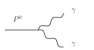
Figure 1: Local contribution to the $P^{0}\to\gamma\gamma$ decay.

$$\mathcal{M}_{\text{Loc}} = i\varepsilon^{\mu\nu\rho\sigma}{q_{1}}_{\mu}{q_{2}}_{\nu}{\epsilon^{*}_{1}}_{\rho}{\epsilon^{*}_{2}}_{\sigma}\frac{2e^{2}}{3F}\times$$ (12)

$$\left\{-\left[\frac{N_{C}}{8\pi^{2}}+8(q_{1}^{2}+q_{2}^{2})C_{22}^{W}\right]C_{P_{0}}+32C_{7}^{W}C_{P_{7}}+64C_{8}^{W}C_{P_{8}}\right\},\;\;$$

where the constants $C_{P_{0}}$, $C_{P_{7}}$ and $C_{P_{8}}$ depend on the pseudo-Goldstone boson considered and are given in table 4.

	$C_{P_{0}}$	$C_{P_{7}}$	$C_{P_{8}}$
$\pi$	1	$m_{\pi}^{2}$	0
$\eta$	$\left({5C_{q}-\sqrt{2}C_{s}}\right)/{3}$	$\left({5C_{q}m_{\pi}^{2}-\sqrt{2}C_{s}\Delta_{2K\pi}^{2}}\right)/{3}$	$2C_{q}m_{\pi}^{2}-\sqrt{2}C_{s}\Delta_{2K\pi}^{2}$
$\eta^{\prime}$	$\left({5C_{q}^{\prime}+\sqrt{2}C_{s}^{\prime}}\right)/{3}$	$\left({5C_{q}^{\prime}m_{\pi}^{2}+\sqrt{2}C_{s}^{\prime}\Delta_{2K\pi}^{2}}\right)/{3}$	$2C_{q}^{\prime}m_{\pi}^{2}+\sqrt{2}C_{s}^{\prime}\Delta_{2K\pi}^{2}$

Table 4: Values of $C_{P_{i}}$ for the local interaction.

The contributions involving one vector resonance exchange (fig. 2) are

$$\mathcal{M}_{1R} = -i\varepsilon^{\mu\nu\rho\sigma}{q_{1}}_{\mu}{q_{2}}_{\nu}{\epsilon_{1}^{*}}_{\rho}{\epsilon_{2}^{*}}_{\sigma}\frac{4\sqrt{2}e^{2}}{3M_{V}F}\times$$

$$\sum_{i=\rho^{0},\omega,\phi}C_{V_{i}}\left\{\frac{4c_{3}(C_{1R}^{m})_{i}+(C_{1R}^{d})_{i}\left[q_{1}\cdot q_{2}(c_{1}+c_{2}-c_{5})+q_{1}^{2}(c_{2}-c_{6})+q_{2}^{2}c_{1}\right]}{M_{i}^{2}-q_{1}^{2}}+(q_{1}\leftrightarrow q_{2})\right\},$$

where the constants $C_{V}$ are

$$C_{V_{i}}=\left\{\begin{array}[]{cc}\frac{1}{3}(F_{V}+8m_{\pi}^{2}\lambda_{V})&\text{for }\omega,\\ (F_{V}+8m_{\pi}^{2}\lambda_{V})&\text{for }\rho^{0},\\ \frac{\sqrt{2}}{3}\left(F_{V}+8\Delta_{2K\pi}^{2}\lambda_{V}\right)&\text{for }\phi,\\ \end{array}\right.$$ (17)

and the constants $C_{1R}^{d}$ and $C_{2R}^{m}$ are given in table 5.

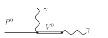
Figure 2: Contribution to the $P^{0}\to\gamma\gamma$ decay with one resonance exchange.

$C_{1R}^{d}$	$\omega$	$\rho^{0}$	$\phi$
$\pi^{0}$	3	1	0
$\eta$	$C_{q}$	$3C_{q}$	$-2C_{s}$
$\eta^{\prime}$	$C_{q}^{\prime}$	$3C_{q}^{\prime}$	$2C_{s}^{\prime}$

$C_{1R}^{m}$	$\omega$	$\rho^{0}$	$\phi$
$\pi^{0}$	$3m_{\pi}^{2}$	$m_{\pi}^{2}$	0
$\eta$	$m_{\pi}^{2}C_{q}$	$3m_{\pi}^{2}C_{q}$	$-2\Delta_{2K\pi}^{2}C_{s}$
$\eta^{\prime}$	$m_{\pi}^{2}C_{q}^{\prime}$	$3m_{\pi}^{2}C_{q}^{\prime}$	$2\Delta_{2K\pi}^{2}C_{s}^{\prime}$

Table 5: Values of $C_{1R}^{d}$ (left) and $C_{1R}^{m}$ (right) for the couplings between different mesons.

The two-vector meson exchange contributions (fig. 3) are given by

$$\mathcal{M}_{2R} = i\varepsilon^{\mu\nu\rho\sigma}{q_{1}}_{\mu}{q_{2}}_{\nu}{\epsilon_{1}^{*}}_{\rho}{\epsilon_{2}^{*}}_{\sigma}\frac{2\sqrt{2}e^{2}}{F}\times$$

$$\sum_{i,j=\rho^{0},\omega,\phi}C_{Vi}C_{Vj}\frac{8d_{2}(C_{2R}^{m})_{ij}+(C_{2R}^{d})_{ij}\left[2(d_{1}-d_{3})q_{1}\cdot q_{2}+d_{1}(q_{1}^{2}+q_{2}^{2})\right]}{(M_{i}^{2}-q_{1}^{2})(M_{j}^{2}-q_{2}^{2})},$$

where the values for the constants $C_{2R}^{d}$ and $C_{2R}^{m}$ can be read from table 6.

$C_{2R}^{d}$	$\omega\omega$	$\rho^{0}\rho^{0}$	$\omega\rho^{0}$	$\phi\phi$
$\pi^{0}$	0	0	$\sqrt{2}$	0
$\eta$	$\sqrt{2}C_{q}$	$\sqrt{2}C_{q}$	0	$-2C_{s}$
$\eta^{\prime}$	$\sqrt{2}C_{q}^{\prime}$	$\sqrt{2}C_{q}^{\prime}$	0	$2C_{s}^{\prime}$

$C_{2R}^{m}$	$\omega\omega$	$\rho^{0}\rho^{0}$	$\omega\rho^{0}$	$\phi\phi$
$\pi^{0}$	0	0	$\sqrt{2}m_{\pi}^{2}$	0
$\eta$	$\sqrt{2}m_{\pi}^{2}C_{q}$	$\sqrt{2}m_{\pi}^{2}C_{q}$	0	$-2\Delta_{2K\pi}^{2}C_{s}$
$\eta^{\prime}$	$\sqrt{2}m_{\pi}^{2}C_{q}^{\prime}$	$\sqrt{2}m_{\pi}^{2}C_{q}^{\prime}$	0	$2\Delta_{2K\pi}^{2}C_{s}^{\prime}$

Table 6: Values of $C_{2R}^{m}$ (up) and $C_{2R}^{m}$ (bottom) for the couplings between different mesons.

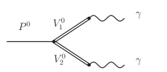
Figure 3: Contribution to the $P^{0}\to\gamma\gamma$ decay with two resonances exchange.

Adding up the various $\pi^{0}\to\gamma^{\star}\gamma^{\star}$ contributions we obtain the $\pi^{0}$-TFF,

$$\mathcal{F}_{\pi^{0}\gamma^{\star}\gamma^{\star}}(q_{1}^{2},q_{2}^{2}) = \frac{2}{3F_{\pi}}\left\{-\frac{N_{C}}{8\pi^{2}}+32m_{\pi}^{2}C_{7}^{W}+\left[-8q_{1}^{2}{C_{22}^{W}}\frac{}{}\right.\right.$$ (19)

$$+\frac{2(F_{V}+8m_{\pi}^{2}\lambda_{V})^{2}\left(d_{3}(q_{1}^{2}+q_{2}^{2})+d_{123}m_{\pi}^{2}\right)}{D_{\rho}(q_{1}^{2})D_{\omega}(q_{2}^{2})}$$

$$-\frac{\sqrt{2}(F_{V}+8m_{\pi}^{2}\lambda_{V})}{M_{V}}\left(m_{\pi}^{2}c_{1235}-q_{1}^{2}c_{1256}+q_{2}^{2}c_{125}\right)\times$$

$$\left(\frac{1}{D_{\rho}(q_{1}^{2})}+\frac{1}{D_{\omega}(q_{1}^{2})}\right)\left.\left.\frac{}{}+\left(q_{1}\leftrightarrow q_{2}\right)\right]^{\frac{}{}}\right\},$$

where $D_{R}(s)=M_{R}^{2}-s$. Note that the pion wave-function renormalization changes the global $F^{-1}$ factor to $F_{\pi}^{-1}$ in the large–$N_{C}$ limit [55, 56, 57].

For simplicity, in addition to the couplings $c_{3}$ and $d_{2}$, we will use the following combinations of constants:

$$c_{1235} =c_{1}+c_{2}+8c_{3}-c_{5},$$ (20a)

$$c_{1256} =c_{1}-c_{2}-c_{5}+2c_{6},$$ (20b)

$$c_{125} =c_{1}-c_{2}+c_{5},$$ (20c)

$$d_{123} =d_{1}+8d_{2}-d_{3}.$$ (20d)

For the $\eta$ meson we find the TFF,

$$\mathcal{F}_{\eta\gamma^{\star}\gamma^{\star}}(q_{1}^{2},q_{2}^{2}) = \frac{2}{3F}\left\{-\frac{\left(5C_{q}-\sqrt{2}C_{s}\right)}{3}\left[8(q_{1}^{2}+q_{2}^{2})C_{22}^{W}+\frac{N_{C}}{8\pi^{2}}\right]\right.$$ (21)

$$+32C_{7}^{W}\frac{5C_{q}m_{\pi}^{2}-\sqrt{2}C_{s}\Delta_{2K\pi}^{2}}{3}+64C_{8}^{W}\left(2C_{q}m_{\pi}^{2}-\sqrt{2}C_{s}\Delta_{2K\pi}^{2}\right)$$

$$+\left[-\frac{\sqrt{2}C_{q}}{3M_{V}}\frac{(F_{V}+8m_{\pi}^{2}\lambda_{V})\left(-8c_{3}\Delta_{\eta\pi}^{2}+c_{1235}m_{\eta}^{2}-c_{1256}q_{1}^{2}+c_{125}q_{2}^{2}\right)}{D_{\rho}(q_{1}^{2})}\right.$$

$$-\frac{3\sqrt{2}C_{q}}{M_{V}}\frac{(F_{V}+8m_{\pi}^{2}\lambda_{V})\left(-8c_{3}\Delta_{\eta\pi}^{2}+c_{1235}m_{\eta}^{2}-c_{1256}q_{1}^{2}+c_{125}q_{2}^{2}\right)}{D_{\omega}(q_{1}^{2})}$$

$$+\frac{4C_{s}}{3M_{V}}\frac{(F_{V}+8\Delta_{2K\pi}^{2}\lambda_{V})\left(c_{1235}m_{\eta}^{2}-c_{1256}q_{1}^{2}+c_{125}q_{2}^{2}+8c_{3}\Delta_{2K\pi\eta}^{2}\right)}{D_{\phi}(q_{1}^{2})}$$

$$+\frac{3C_{q}(F_{V}+8m_{\pi}^{2}\lambda_{V})^{2}\left(-8d_{2}\Delta_{\eta\pi}^{2}+d_{123}m_{\eta}^{2}+d_{3}(q_{1}^{2}+q_{2}^{2})\right)}{D_{\rho}\left(q_{1}^{2}\right)D_{\rho}\left(q_{2}^{2}\right)}$$

$$+\frac{C_{q}(F_{V}+8m_{\pi}^{2}\lambda_{V})^{2}\left(-8d_{2}\Delta_{\eta\pi}^{2}+d_{123}m_{\eta}^{2}+d_{3}(q_{1}^{2}+q_{2}^{2})\right)}{3D_{\omega}\left(q_{1}^{2}\right)D_{\omega}\left(q_{2}^{2}\right)}$$

$$-\frac{2\sqrt{2}C_{s}(F_{V}+8\Delta_{2K\pi}^{2}\lambda_{V})^{2}\left(d_{123}m_{\eta}^{2}+d_{3}(q_{1}^{2}+q_{2}^{2})+8d_{2}\Delta_{2K\pi\eta}^{2}\right)}{3D_{\phi}\left(q_{1}^{2}\right)D_{\phi}\left(q_{2}^{2}\right)}$$

$$\left.\left.\frac{}{}+(q_{1}\leftrightarrow q_{2})^{\frac{}{}}\right]^{\frac{}{}}\right\},$$

where $\Delta_{\eta\pi}^{2}=m_{\eta}^{2}-m_{\pi}^{2}$ and $\Delta_{2K\pi\eta}^{2}=2m_{K}^{2}-m_{\pi}^{2}-m_{\eta}^{2}$. The result for the $\eta^{\prime}$ can be obtained from the previous one by substituting $C_{q}\to C_{q}^{\prime}$, $C_{s}\to-C_{s}^{\prime}$ and $m_{\eta}\to m_{\eta^{\prime}}$. Notice that by taking the chiral limit one recovers the expressions given previously in refs. [41, 42].

We would like to remark that the value of pseudoscalar decay constant in the chiral limit, $F$, is not required in our R$\chi$T description. In the $\pi^{0}$-TFF it combines into the global $F_{\pi}^{-1}$ factor in eq. (19), with $F_{\pi}=92.2$ MeV [1]. In the same way, the $\eta$ and $\eta^{\prime}$ form-factors only depend on the combinations $C_{q}/F$, $C_{s}/F$, $C_{q}^{\prime}/F$ and $C_{s}^{\prime}/F$ which, in turn, only depend on the mixing angles $\theta_{8}$, $\theta_{0}$ and the value of $f_{8}$ and $f_{0}$ (not on their ratios $f_{8}/F$ and $f_{0}/F$).

Since we want to make use of the $VVP$ Green’s function short-distance constraints [41], the analysis is incomplete if the pseudoscalar resonance multiplet, $P^{\prime}$, –included in ref. [41]– is not considered. The $d_{m}$ operator introduces a mixing between $P^{\prime}$ and the pseudo-Goldstone states $P$ proportional to the quark masses. Thus, the contributions from the heavy pseudoscalar nonet to the $P$–TFFs begin at ${\cal O}(m_{P}^{2})$ and, at that order, take the form

$$\mathcal{F}_{P\to P^{{}^{\prime}\star}\to\gamma^{\star}\gamma^{\star}} = C_{P_{7}}\,\times\,\frac{\displaystyle 2\sqrt{2}d_{m}}{\displaystyle FM_{P^{\prime}}^{2}}\,\mathcal{F}_{P_{I=1}^{{}^{\prime}\star}(p)\to\gamma^{\star}\gamma^{\star}}\bigg{|}_{p^{2}\to 0}\,,$$ (22)

in terms of the $P^{\prime\star}(p)\to\gamma^{\star}(q_{1})\gamma^{\star}(q_{2})$ transition amplitude in the chiral and large–$N_{C}$ limits, provided here for the isospin $I=1$ resonance by

$$\mathcal{F}_{P_{I=1}^{{}^{\prime}\star}(p)\to\gamma^{\star}\gamma^{\star}} = \frac{8\sqrt{2}}{3}\left[4\kappa_{5}^{P}-\sqrt{2}\kappa_{3}^{PV}F_{V}\left(\frac{1}{M_{V}^{2}-q_{1}^{2}}+\frac{1}{M_{V}^{2}-q_{2}^{2}}\right)\right.$$ (23)

$$\qquad\qquad\left.+\frac{\kappa^{PVV}F_{V}^{2}}{(M_{V}^{2}-q_{1}^{2})(M_{V}^{2}-q_{2}^{2})}\right]\,,$$

where $C_{P_{7}}={\cal O}(m_{P}^{2})$ and $M_{P^{\prime}}$ is the $P^{\prime}$ mass in the chiral and large–$N_{C}$ limits. $U(3)$ breaking effects in the $P^{\prime}$ multiplet would contribute to our $P$–TFFs at higher orders in $m_{P}^{2}$. This result for the off-shell $P^{{}^{\prime}\star}\gamma^{\star}\gamma^{\star}$ transition is in agreement with ref. [41] and the $U(3)$ limit of eq. (22) (given by $m_{\pi}=m_{K}$ in $C_{P_{7}}$) coincides with $U(3)$ symmetric contribution to the $P$–TFFs in ref. [42]. Comparing these expressions for the $P^{\prime}$ contributions with those in eqs. (19) and (21), it becomes evident that these contributions can be included merely by a redefinition of three parameters, namely, $C_{7}^{W}$, $c_{3}$, $d_{2}$: 

$$C_{7}^{W}\,\,\longrightarrow\,\,{C_{7}^{W}}^{\star} =C_{7}^{W}+\frac{2d_{m}\kappa_{5}^{P}}{M_{P^{\prime}}^{2}}\,,$$ (24a)

$$c_{3}\,\,\longrightarrow\,\,\,\,\,\,c_{3}^{\star}\,\, =c_{3}+\frac{d_{m}M_{V}\kappa_{3}^{PV}}{M_{P^{\prime}}^{2}}\,,$$ (24b)

$$d_{2}\,\,\longrightarrow\,\,\,\,\,\,d_{2}^{\star}\,\, =d_{2}+\frac{d_{m}\kappa^{PVV}}{2M_{P^{\prime}}^{2}}\,.$$ (24c)

Note that the R$\chi$T couplings $c_{1,2,5,6}$ and $d_{1,3}$ do not need to be corrected. However, in order to take the $P^{\prime}$ contributions into account, we will also need to shift our auxiliary combinations

$$c_{1235}\,\,\longrightarrow\,\, c_{1235}^{\star}=c_{1}+c_{2}+8c_{3}^{\star}-c_{5}\,,$$ (25a)

$$d_{123}\,\,\longrightarrow\,\, d_{123}^{\star}=d_{1}+8d_{2}^{\star}-d_{3}\,.$$ (25b)

4 Short Distance Constraints

We will constrain the R$\chi$T parameters by imposing on the $\mathcal{F}_{P\gamma^{\star}\gamma^{\star}}$ TFFs ($P=\pi^{0},\eta,\eta^{\prime}$) the high energy behaviour prescribed by QCD [45, 61]:

$$\mathcal{F}_{P\gamma^{\star}\gamma^{\star}}(q^{2},q^{2})\,\,\stackrel{{\scriptstyle Q^{2}\to\infty}}{{\longrightarrow}}\,\,0\,,\qquad\qquad\ \mathcal{F}_{P\gamma^{\star}\gamma^{\star}}(q^{2},0)\,\,\stackrel{{\scriptstyle Q^{2}\to\infty}}{{\longrightarrow}}\,\,0\,,$$ (26)

with $Q^{2}=-q^{2}$. These conditions are applied order by order in the $m_{P}^{2}$ expansion, separately: first in the massless limit, at ${\cal O}(m_{P}^{0})$, and then at ${\cal O}(m_{P}^{2})$. We emphasize that in this work we are not matching the precise QCD predictions for the coefficients of the $1/Q^{2}$ expansion [45, 61], just requiring the vanishing of the TFF at high momentum transfer. We will see that these results are found to be compatible with previous results [41, 50] from the analysis of the VVP Green’s function and other observables. The constraints from ${\cal O}(m_{P}^{4})$ or higher are not taken into account, as we did not considered R$\chi$T operators contributing at that order.

The high-energy analysis of the TFF leads to the relations:

• $\pi^{0}$-TFF, $\hskip 4.30554pt{\cal O}(m_{P}^{0})$ :

  $$C_{22}^{W}= \,0,$$ (27a)

  $$c_{125}= \,0,$$ (27b)

  $$c_{1256}= -\frac{N_{C}M_{V}}{32\sqrt{2}\pi^{2}F_{V}},$$ (27c)

  $$d_{3}= -\frac{N_{C}M_{V}^{2}}{64\pi^{2}F_{V}^{2}}.$$ (27d)

• $\pi^{0}$-TFF, $\hskip 4.30554pt{\cal O}(m_{P}^{2})$ :

  $$\lambda_{V}= -\frac{32\pi^{2}F_{V}}{N_{C}}C_{7}^{W\star}\,,$$ (28a)

  $$c_{1235}^{\star}= \frac{N_{C}M_{V}e_{m}^{V}}{8\sqrt{2}\pi^{2}F_{V}}+\frac{\displaystyle N_{C}M_{V}^{3}\lambda_{V}}{\displaystyle 4\sqrt{2}\pi^{2}F_{V}^{2}}\,.$$ (28b)

• Additional $\eta$-TFF constraints, ${\cal O}(m_{P}^{2})$:

  $$C_{8}^{W}= \,0,$$ (29a)

  $$c_{3}^{\star}= \frac{c_{1235}^{\star}}{8}=\frac{N_{C}M_{V}e_{m}^{V}}{64\sqrt{2}\pi^{2}F_{V}}+\frac{\displaystyle N_{C}M_{V}^{3}\lambda_{V}}{\displaystyle 32\sqrt{2}\pi^{2}F_{V}^{2}}\,.$$ (29b)

  Notice that the implicit $\kappa_{3}^{PV}$ cancels out in the last equation so it should be actually read as $c_{3}=c_{1235}/8$. This, in combination with the constraint (27b), yields $c_{1}=c_{2}-c_{5}=0$.

• No additional $\eta^{\prime}$-TFF constraints: up to ${\cal O}(m_{P}^{2})$, the analysis of the $\eta^{\prime}$-TFF casts the same relations provided by the $\pi^{0}$ and $\eta$ form-factors.

We note that we did not need to perform the $m_{P}^{2}$ expansion of the mixing coefficients $C_{q/s}^{(^{\prime})}$. One obtains the previous set of consistent relations for any value of $C_{q/s}^{(^{\prime})}$: our conditions are actually requiring a good high-energy behaviour to the bare $\phi^{a}\to\gamma^{\star}\gamma^{\star}$ TFFs, which is inherited by the physical $\pi^{0}$, $\eta$ and $\eta^{\prime}$ TFFs after taking into account the field renormalizations and mixings provided by $C_{\pi}$ and $C_{q/s}^{(^{\prime})}$.

This allows us to by-pass the cumbersome problem of the large–$N_{C}$ limit in the $\eta-\eta^{\prime}$ mixing [52], where $1/N_{C}$ and quark mass corrections are found to be of a similar numerical order [52, 53, 59].

We will supplement these TFF constraints with the additional conditions derived from the short-distance analysis of the VVP Green’s function $\Pi(p^{2},q^{2},r^{2})$ [41]. By matching the leading terms of the QCD OPE at $p^{2},q^{2},r^{2}\to\infty$ within the chiral and large–$N_{C}$ limits, ref. [41] obtains ,

• $VVP$ Green’s function, $\hskip 4.30554pt{\cal O}(m_{P}^{0})$ :

  $$c_{125}\,=\,c_{1235}\,=\,0\,,\qquad c_{1256}=-\frac{\displaystyle N_{C}M_{V}}{\displaystyle 32\sqrt{2}\pi^{2}F_{V}}\,,$$

  $$d_{3}\,=\,-\frac{\displaystyle N_{C}M_{V}^{2}}{\displaystyle 64\pi^{2}F_{V}^{2}}+\frac{\displaystyle F^{2}}{\displaystyle 8F_{V}^{2}}+\frac{\displaystyle 4\sqrt{2}d_{m}\kappa_{3}^{PV}}{\displaystyle F_{V}}\,,\qquad d_{123}\,=\,\frac{\displaystyle F^{2}}{\displaystyle 8F_{V}^{2}}\,,\qquad\kappa_{5}^{P}\,=\,0\,,$$

  $$C_{7}^{W}\,=\,C_{8}^{W}\,=\,C_{22}^{W}\,=\,0\,.$$ (30)

In the last line, we added the VVP constraints for the R$\chi$T couplings $C_{j}^{W}$ in $\mathcal{L}_{\rm non-R}$. It is remarkable that these relations are compatible with our TFF relations above, being the relations for $c_{125}$, $c_{1256}$, $C_{8}^{W}$ and $C_{22}^{W}$ identical. Combining these VVP constraints [41] with the previous ones from the high-energy TFF analysis up to ${\cal O}(m_{P}^{2})$, we conclude the constraints

$$c_{1}\,=\,c_{2}-c_{5}\,=\,c_{3}\,=\,c_{125}\,=\,c_{1235}\,=\,0\,,$$

$$c_{1235}^{\star}\,=\,8c_{3}^{\star}\,=\,\,\frac{\displaystyle 8d_{m}\kappa_{3}^{PV}M_{V}}{\displaystyle M_{P^{\prime}}^{2}}\,=\,\frac{\displaystyle N_{C}e_{m}^{V}M_{V}}{\displaystyle 8\sqrt{2}\pi^{2}F_{V}}\,,$$

$$d_{123}^{\star}\,=\,\frac{\displaystyle F^{2}}{\displaystyle 8F_{V}^{2}}+\frac{\displaystyle 4d_{m}\kappa^{PVV}}{\displaystyle M_{P^{\prime}}^{2}}\,,\qquad\qquad d_{123}\,=\,\frac{\displaystyle F^{2}}{\displaystyle 8F_{V}^{2}}\,,$$

$$d_{3}=-\frac{N_{C}M_{V}^{2}}{64\pi^{2}F_{V}^{2}}\,,\qquad\qquad c_{1256}=-\frac{\displaystyle N_{C}M_{V}}{\displaystyle 32\sqrt{2}\pi^{2}F_{V}}\,,$$

$${C_{7}^{W}}^{\star}\,=\,\lambda_{V}=0\,,\qquad\kappa_{5}^{P}=0\,,\qquad C_{7}^{W}={C_{8}^{W}}=C_{22}^{W}=0.$$ (31)

The relations obtained in this way fix all the parameters in the form-factors except for $d_{123}^{\star}$, $d_{2}^{\star}$, $M_{V}$, $e_{m}^{V}$ and the four $\eta-\eta^{\prime}$ mixing parameters. Particularly, among the operators violating $U(3)$ explicitly, those with coefficients $c_{3}$, ${C_{7}^{W}}^{\star}$, $C_{8}^{W}$ and $\lambda_{V}$ vanish, according to eq. (31). Although there is a relation for $d_{123}$ from the OPE study of the VVP Green’s function, $d_{123}^{\star}$ is not well known since the $\kappa^{PVV}$ coupling remains unconstrained [41]. The unrestricted parameters are fitted in this work using $\mathcal{F}_{P\gamma^{\star}\gamma^{\star}}(q^{2},0)$ experimental data for $\pi^{0}$, $\eta$ and $\eta^{\prime}$. The results are given in the next section. There is one more constraint for $\kappa_{3}^{PV}$ from the combination of the TFF and VVP relations for $d_{3}$ in the chiral and large–$N_{C}$ limits [41], which, however will not be considered in detail in this work:

$$8d_{m}\kappa_{3}^{PV}\,=\,-\frac{\displaystyle F^{2}}{\displaystyle 4\sqrt{2}F_{V}}\,<\,0\,.$$ (32)

In principle, this, together with the previous constraints, leads to a negative vector mass splitting parameter $e_{m}^{V}$, in agreement with previous phenomenology [39] and our later fits. This prediction $e_{m}^{V}=-2\pi^{2}F^{2}/(N_{C}M_{P^{\prime}}^{2})$ is, however, one order of magnitude smaller for $F\sim F_{\pi}$ and $M_{P^{\prime}}\sim 1.3$ GeV than the values required by the phenomenology. Nonetheless, one should be very cautious with the theoretical determinations of the $P^{\prime}$ couplings: under the lightest $P^{\prime}$ and $V$ resonance multiplet approximation it is possible to obtain a good high-energy behaviour for the $\pi^{0}$–TFF and VVP Green’s function in the chiral limit but at the price of a $P^{\prime}\to\gamma^{\star}\gamma$ TFF (23) which does not vanish a large momentum transfer. For this reason we have decided to leave $\kappa_{3}^{PV}$ –or equivalently $e_{m}^{V}$– as a phenomenological parameter in our later fits, postponing further studies on the structure of the $P^{\prime}$ Lagrangian for a future work.

After using the SD constraints, the $\pi^{0}$-TFF results simplified into the form

$$\mathcal{F}_{\pi\gamma^{\star}\gamma^{\star}}(q_{1}^{2},q_{2}^{2})=\frac{32\pi^{2}m_{\pi}^{2}F_{V}^{2}d_{123}^{\star}-N_{C}M_{V}^{2}M_{\rho}^{2}}{12\pi^{2}F_{\pi}D_{\rho}(q_{1}^{2})D_{\rho}(q_{2}^{2})},$$ (33)

Also the $\eta$-TFF is simplified to

$$\mathcal{F}_{\eta\gamma^{\star}\gamma^{\star}}(q_{1}^{2},q_{2}^{2}) = \frac{1}{12\pi^{2}FD_{\rho}(q_{1}^{2})D_{\rho}(q_{2}^{2})D_{\phi}(q_{1}^{2})D_{\phi}(q_{2}^{2})}\times$$

$$\left\{-\frac{N_{C}M_{V}^{2}}{3}\left[5C_{q}M_{\rho}^{2}D_{\phi}(q_{1}^{2})D_{\phi}(q_{2}^{2})-\sqrt{2}C_{s}M_{\phi}^{2}D_{\rho}(q_{1}^{2})D_{\rho}(q_{2}^{2})\right]\right.$$

$$+\frac{32\pi^{2}F_{V}^{2}d_{123}^{\star}m_{\eta}^{2}}{3}\left[(5C_{q}D_{\phi}(q_{1}^{2})D_{\phi}(q_{2}^{2})-\sqrt{2}C_{s}D_{\rho}(q_{1}^{2})D_{\rho}(q_{2}^{2})\right]$$

$$\left.-\frac{256\pi^{2}F_{V}^{2}d_{2}^{\star}}{3}\left[(5C_{q}\Delta_{\eta\pi}^{2}D_{\phi}(q_{1}^{2})D_{\phi}(q_{2}^{2})+\sqrt{2}C_{s}\Delta_{2K\pi\eta}^{2}D_{\rho}(q_{1}^{2})D_{\rho}(q_{2}^{2})\right]\right\}.$$

The constrained $\eta^{\prime}$-TFF is given by this expression with the same replacements indicated before after eq. (21): $C_{q}\to C_{q}^{\prime}$, $C_{s}\to-C_{s}^{\prime}$ and $m_{\eta}\to m_{\eta^{\prime}}$.

In the chiral and large–$N_{C}$ limits one has $m_{P}\to 0$ and we recover the previous result from ref. [43]:

$$\mathcal{F}_{\pi^{0}\gamma^{\star}\gamma^{\star}}(q_{1}^{2},q_{2}^{2}) = \,-\,\frac{\displaystyle N_{C}M_{V}^{4}}{\displaystyle 12\pi^{2}F(M_{V}^{2}-q_{1}^{2})(M_{V}^{2}-q_{2}^{2})}\,,$$ (35)

and $\mathcal{F}_{\eta\gamma^{\star}\gamma^{\star}}(q_{1}^{2},q_{2}^{2})=\mathcal{F}_{\pi^{0}\gamma^{\star}\gamma^{\star}}(q_{1}^{2},q_{2}^{2})\times(5C_{q}-\sqrt{2}C_{s})/3$. The result for the $\eta^{\prime}$ TFF is analogous with $C_{q}\to C_{q^{\prime}}$ and $C_{s}\to-C_{s^{\prime}}$ [42] . We find again at ${\cal O}(m_{P}^{2})$ the issue pointed out in previous studies of the TFF with only one vector multiplet at ${\cal O}(m_{P}^{0})$ [43]: it is not possible to match the $1/q^{2}$ coefficient prescribed by QCD at deep virtual momentum $Q^{2}\to\infty$ at the same time for both kinematical configurations $\mathcal{F}_{P\gamma^{\star}\gamma^{\star}}(q^{2},0)\approx 2F/q^{2}$ [45] and $\mathcal{F}_{P\gamma^{\star}\gamma^{\star}}(q^{2},q^{2})\approx 2F/(3q^{2})$ [61]. We will see that, even though the first limit is not imposed, our TFFs fitted to data approximately recover the asymptotic behaviour $2F/q^{2}$. On the other hand, for the doubly off-shell TFFs we always find $\mathcal{F}_{P\gamma^{\star}\gamma^{\star}}(q^{2},q^{2})\stackrel{{\scriptstyle Q^{2}\to\infty}}{{=}}{\cal O}(1/q^{4})$. This deficiency of our description might lead to a slight underestimation of our result for $a_{\mu}^{P,HLbL}$ that will be later discussed.

We would like to remark that the $P\gamma^{\star}\gamma^{\star}$ and $VVP$ short-distance relations provided here are fully compatible with the constraints from $\tau\to P^{-}\gamma\nu_{\tau}$ [62] and $\tau\to(PV)^{-}\nu_{\tau}$ [63]. The high-energy conditions from $\tau\to(KK\pi)^{-}\nu_{\tau}$ [64] and $\tau\to\eta\pi^{-}\pi^{0}\nu_{\tau}$ [65] are also compatible with the relations in the present article provided $F_{V}=\sqrt{3}F$ [50]. Nevertheless, the outcomes in this article will not rely on this last relation, even though it will be useful for comparison.

5 Form factor experimental data analysis

5.1 Fit to experimental TFF

After demanding the high-energy TFF and $VVP$ conditions, these form-factors depend only on the vector mass parameters $M_{V}$ and $e_{m}^{V}$, the combinations $F_{V}^{2}d_{123}^{\star}$ and, in the $\eta$ and $\eta^{\prime}$ cases, $F_{V}^{2}d_{2}^{\star}$ and the coefficients $C_{q/s}^{(^{\prime})}/F$ (which only depend on the mixing parameters $\theta_{8}$, $\theta_{0}$, $f_{8}$ and $f_{0}$) . All fitted parameters (but $M_{V}$) break explicitly the $U(3)$ flavor symmetry.

We will determine these 8 parameters by means of a fit to the available space-like experimental data. Notice, however, that our fit will be completely insensitive to $F_{V}$, since it only appears in the form-factors multiplying $d_{2}^{\star}$ and $d_{123}^{\star}$. Therefore, for convenience and to ease the comparison we will show the results for the combinations

$$\bar{d}_{2}\equiv\frac{\displaystyle F_{V}^{2}d_{2}^{\star}}{\displaystyle 3F_{\pi}^{2}}\,,\qquad\bar{d}_{123}\equiv\frac{\displaystyle F_{V}^{2}d_{123}^{\star}}{\displaystyle 3F_{\pi}^{2}}\,,$$ (36)

with $F_{\pi}=92.2$ MeV [1].

Since we are mainly focused on the application of the transition Form Factor in the pseudoscalar exchange contribution to the $a_{\mu}^{HLbL}$, we will only perform fits to data with negative squared photon momenta, $q^{2}\leq 0$. There are two reasons for this, the first one is that being a NLO effect in the $1/N_{C}$ expansion, the width of the resonances is needed to obtain a finite result in the $q^{2}>0$ region of momenta, and to be consistent, we would need to consider also all NLO terms in the $1/N_{C}$ expansion; the other one is that the observables in the time-like region may get large contributions from disregarded photon radiative corrections [47].

The $\Gamma(P\to\gamma\gamma)$ decay widths give relevant information of the form-factor at very low energies and help reduce the error in the $\eta-\eta^{\prime}$ mixing parameters. The values for the $\Gamma(P\to\gamma\gamma)$ decays are taken from the Particle Data Group (PDG) [1]. The relation between the form-factor and the on-shell photons decay width is given by

$$|\mathcal{F}_{P\gamma^{\star}\gamma^{\star}}(0,0)|^{2}=\frac{64\pi}{(4\pi\alpha)^{2}}\frac{\Gamma(P\to\gamma\gamma)}{m_{P}^{3}}.$$ (37)

We use CLEO [66], CELLO [67], LEP [68], BaBar [44, 69] and Belle [70] data of the form-factors along with the decay width to real photons. Since the PDG takes into account LEP data at $q^{2}=0$ for the $\eta^{\prime}\to\gamma\gamma$ transition, we have removed this bin to avoid double counting. We fit our form-factors for $\pi^{0}$, $\eta$ and $\eta^{\prime}$ to all these data, simultaneously.

In order to stabilize the fit, we have added a contribution to the $\chi^{2}$ given by the values of the parameters $\theta_{8/0}$ and $f_{8/0}$ from previous determinations [52, 53, 58], namely

$$\theta_{8}= (-21.2\pm 1.6)^{\circ},$$ (38a)

$$\theta_{0}= (-9.2\pm 1.7)^{\circ},$$ (38b)

$$f_{8}= (1.26\pm 0.04)F_{\pi}=(116.2\pm 3.7)\mathrm{\hskip 4.30554ptMeV},$$ (38c)

$$f_{0}= (1.17\pm 0.03)F_{\pi}=(107.9\pm 2.8)\mathrm{\hskip 4.30554ptMeV}.$$ (38d)

This gives a very small contribution $\Delta\chi^{2}\approx 1.5$. These inputs could be understood as a prior distribution for the mixing parameters given by [52, 53, 58]. If one, however, takes the numbers given in ref. [59] , $f_{0}$ and $\theta_{0}$ coincide with the results of our best fit in table 7, but we get $\theta_{8}=(-23.8\pm 0.9)^{\circ}$ and $f_{8}=(151\pm 9)$ MeV, which is no longer compatible with the results from table 7. Also, since $e_{m}^{V}$ and $M_{V}$ are correlated to the mixing parameters, these values change to $M_{V}=(777\pm 10)$ MeV and $e_{m}^{V}=(-51\pm 17)\cdot 10^{-2}$. This input rises the $\chi^{2}$ by $\sim 12$. Despite the different values of these parameters, we get a value for $a_{\mu}^{P,HLbL}$ still compatible with the result from our best fit (see section 7). If one uses $F$ instead of $F_{\pi}$ in eqs. (38c) and (38d), the values for the parameters are completely compatible with those from our best fit. With this input we also get a result compatible with our best fit $a_{\mu}^{P,HLbL}$ (see secs. 6 and 7). If, furthermore, we remove the stabilizing conditions, eqs. (38a)–(38d), we end up with values for the mixing parameters that are incompatible with previous determinations [52, 53, 58, 59]: $\theta_{8}=(-27\pm 4)^{\circ}$, $\theta_{0}=(-5\pm 8)^{\circ}$, $f_{8}=(220\pm 40)$ MeV and $f_{0}=(110\pm 30)$ MeV (though this leads to $a_{\mu}^{P,HLbL}=(8.81\pm 0.16)\cdot 10^{-10}$, compatible with our best fit in secs. 6 and 7). The reason for this is that, as can be seen in table 8 (and tables 14 and 15), there is a large correlation between $\mathcal{P}_{1}$ and $\theta_{8}$ and between $\mathcal{P}_{2}$ and $\theta_{0}$ and $f_{0}$ (in addition to the strong correlations between the four mixing parameters) . Therefore, the fit to the TFF data alone is not really sensitive to the four mixing parameters but to combinations of them and $\mathcal{P}_{1,2}$. The stabilizing conditions in eq. (38) lessen the effect of such high correlations avoiding, thus, a non-physical region for the mixing parameters.

		(Best Fit)
	‘fit 1’	‘fit 2’	‘fit 3’
	With $\pi^{0}$-BaBar	Without $\pi^{0}$-BaBar	Fixing $M_{V}$ and $e_{m}^{V}$
$\mathcal{P}_{1}$	$-0.2\pm 1.0$	$0.0\pm 1.0$	$0.0\pm 1.0$
$\mathcal{P}_{2}$	$0.5\pm 1.0$	$0.0\pm 0.5$	$0.0\pm 1.0$
$\bar{d}_{2}$	$(-2.9\pm 1.7)\cdot 10^{-2}$	$(-2.7\pm 1.7)\cdot 10^{-2}$	$(-3\pm 2)\cdot 10^{-2}$
$\bar{d}_{123}$	$(-2.5\pm 1.5)\cdot 10^{-1}$	$(-2.3\pm 1.5)\cdot 10^{-1}$	$(-3\pm 2)\cdot 10^{-1}$
$M_{V}$	$(799\pm 5)$ MeV	$(791\pm 6)$ MeV	764.3 MeV †
$e_{m}^{V}$	$-0.35\pm 0.10$	$-0.36\pm 0.10$	$-0.228$ †
$\theta_{8}$	$(-19.5\pm 0.9)^{\circ}$	$(-19.5\pm 0.9)^{\circ}$	$(-21.7\pm 0.9)^{\circ}$
$\theta_{0}$	$(-9.5\pm 1.6)^{\circ}$	$(-9.5\pm 1.6)^{\circ}$	$(-10.4\pm 1.6)^{\circ}$
$f_{8}$	$(118\pm 4)$ MeV	$(118\pm 3)$ MeV	$(118\pm 3)$ MeV
$f_{0}$	$(108\pm 3)$ MeV	$(107.5\pm 1.0)$ MeV	$(107\pm 3)$ MeV
$\chi^{2}$/dof	$150./101$	$69./84$	$101./86$

Table 7: Values for the fitted parameters with (first column) and without (second column) BaBar data on the $\pi^{0}$ form-factor. We fit the parameters $M_{V}$, $e_{m}^{V}$ and the mixing couplings together with $\mathcal{P}_{1}$ and $\mathcal{P}_{2}$, not $\bar{d}_{2}$ and $\bar{d}_{123}$; these are reconstructed from the fitted values for $\mathcal{P}_{1}$ and $\mathcal{P}_{2}$ and eqs. (39a) and (39b) and shown here for illustration. The third column shows the parameters fitted excluding BaBar $\pi^{0}$ data and fixing $M_{V}$ and $e_{m}^{V}$ (marked with $\dagger$) according to refs. [39]. The last row collects the $\chi^{2}$ per degree of freedom (dof).

	$\mathcal{P}_{1}$	$\mathcal{P}_{2}$	$M_{V}$	$e_{m}^{V}$	$\theta_{8}$	$\theta_{0}$	$f_{8}$	$f_{0}$
$\mathcal{P}_{1}$	1	0.085	0.511	0.638	0.495	0.017	-0.107	-0.025
$\mathcal{P}_{2}$	0.085	1	0.434	0.439	-0.157	-0.616	-0.058	0.434
$M_{V}$	0.511	0.434	1	0.444	0.321	-0.054	-0.129	0.351
$e_{m}^{V}$	0.638	0.439	0.444	1	-0.081	0.059	-0.179	0.319
$\theta_{8}$	0.495	-0.157	0.321	-0.081	1	-0.046	-0.486	-0.184
$\theta_{0}$	0.017	-0.616	-0.054	0.059	-0.046	1	-0.020	-0.424
$f_{8}$	-0.107	-0.058	-0.129	-0.179	-0.486	-0.020	1	-0.156
$f_{0}$	-0.025	0.434	0.351	0.319	-0.184	-0.424	-0.156	1

Table 8: Correlation matrix for our best fit (excluding BaBar $\pi^{0}$–TFF data).

We now focus on the fit to TFF data and eqs. (38a)–(38d). A preliminary fit with $f_{8/0}$, $\theta_{8/0}$, $M_{V}$, $e_{m}^{V}$ and $\bar{d}_{2}$ and $\bar{d}_{123}$ shows a correlation between the latter two close to one. Hence, instead of considering $\bar{d}_{2}$ and $\bar{d}_{123}$, we will fit the parameters $\mathcal{P}_{1}$ and $\mathcal{P}_{2}$ provided by the linear combinations

$$\bar{d}_{2}= \alpha_{2}+\frac{\sigma_{d_{2}}}{\sqrt{2}}\left(\sqrt{1+r}\hskip 4.30554pt\mathcal{P}_{1}-\sqrt{1-r}\hskip 4.30554pt\mathcal{P}_{2}\right),$$ (39a)

$$\bar{d}_{123}= \alpha_{123}+\frac{\sigma_{d_{123}}}{\sqrt{2}}\left(\sqrt{1+r}\hskip 4.30554pt\mathcal{P}_{1}+\sqrt{1-r}\hskip 4.30554pt\mathcal{P}_{2}\right),$$ (39b)

with $\alpha_{2}=-0.0272$, $\alpha_{123}=-0.233$, $\sigma_{d_{2}}=10.49\cdot 10^{-3}$, $\sigma_{d_{123}}=81.28\cdot 10^{-3}$ and $r=0.995$. A fair estimate of the constants $\sigma_{d_{2}}$, $\sigma_{d_{123}}$ and $r$ that minimize these fit correlations can be extracted from the errors and correlation between $\bar{d}_{2}$ and $\bar{d}_{123}$, respectively, in the preliminary fit. This transformation greatly reduces the correlation between both fit parameters, improving the efficiency and reliability of the numerical fit. We note that these constants $\sigma_{d_{2}}$, $\sigma_{d_{123}}$ and $r$ will change if one considers a different data set or fixes some parameters, e.g., $M_{V}$ and $e_{m}^{V}$. In this case, the fit to all the available space-like TFF data casts the mean values and errors given in table 7 (first column of results; $\bar{d}_{2,123}$ were reconstructed from $\mathcal{P}_{1,2}$ by means of eqs. (39a) and (39b)). Further details on the correlations for this ‘fit 1’have been relegated to table 14 in App. C.

However, this first fit points out that the $\pi^{0}$ BaBar data [44] is in conflict with $\eta$ and $\eta^{\prime}$-TFF data, related through chiral symmetry, and with Belle data (see e.g. refs. [71, 72, 73, 74, 75, 76, 77, 78, 79]). Likewise, it is at odds with the asymptotic $\pi^{0}$ form-factor behaviour $\mathcal{F}_{\pi^{0}\gamma^{\star}\gamma^{\star}}\sim{\cal O}(Q^{-2})$ expected in high-energy QCD [45]. Indeed, this set of $\pi^{0}$ data is exclusively responsible for the important deviation in $\chi^{2}$ ($150.$) from the number of degrees of freedom of this ‘fit 1’ ($101$). Once the BaBar $\pi^{0}$ data set is removed from the analysis, the ratio $\chi^{2}/$dof drops and our theoretical expressions provide a good description for all the $\pi^{0}$, $\eta$ and $\eta^{\prime}$ experimental data. Thus, we will take this ‘fit 2’ as our best fit. The corresponding mean values and marginal standard deviations are given in table 7 (second column of results) and their correlations can be found in table 8. In order to reduce the correlations in‘fit 2’ ($\pi^{0}$ BaBar data excluded), we have used transformations (39a) and (39b) with the same values for $\sigma_{d_{2}}$, $\sigma_{d_{123}}$ and $r$ as ‘fit 1’ ($\pi^{0}$ BaBar data included).

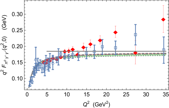
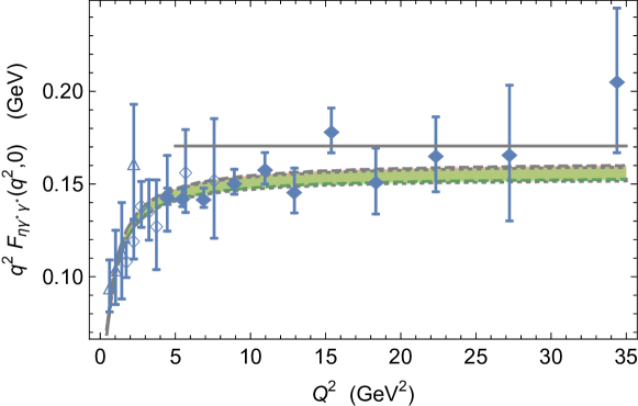
Figure 4: Comparison between the $\pi^{0}$ (top), $\eta$ (middle) and $\eta^{\prime}$ (bottom) TFFs from the fit to all data (darker red band with dashed borders) and the fit after removing BaBar $\pi^{0}$ data (clearer green band with dotted borders). See the text for details.

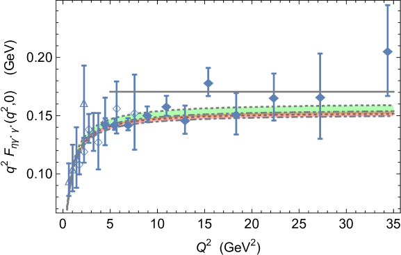
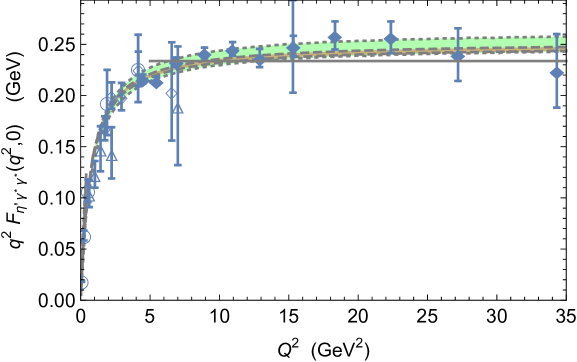
Figure 5: Comparison between the $\pi^{0}$ (top), $\eta$ (middle) and $\eta^{\prime}$ (bottom) TFFs from the fit with $M_{V}$ and $e_{m}^{V}$ fixed (darker red band with dashed borders) and with these parameters included in the fit (clearer green band with dotted borders). BaBar $\pi^{0}$ data is not fitted in both cases. The remaining notation is the same as in fig. 4.

The values of $M_{V}$ obtained from these fits seem rather at odds with what one expects from the measured mass of the lowest-lying resonances: $M_{\rho}=M_{\omega}\approx 807$ MeV and $M_{\phi}\approx 1126$ MeV. In principle, this is not a problem for our analysis, as we are considering a purely space-like analysis within the lightest resonance multiplet and large–$N_{C}$ approximation. Thus, the parameters employed here are not truly those of the full theory with the large–$N_{C}$ infinite tower of resonances. Thus, the lightest vector couplings become slightly shifted to compensate for the heavier resonances missing in our R$\chi$T description. This could mean that resonances from heavier multiplets (e.g., $\rho^{\prime}$) might be giving a contribution to the experimental data of the form-factor which is not fully negligible in our approach. Therefore, we decided to make yet another fit fixing the mass and the $U(3)$ splitting parameter, excluding the $\pi^{0}$ data from BaBar, in order to study how this affects our results. This ‘fit 3’ gives the values shown in the third column of table 7, and the correlation among parameters in table 15 in app. C. As done in the previous fits, the $\bar{d}_{2}$ and $\bar{d}_{123}$ parameters were transformed in the same way, however, for this fit the values of the decorrelating transformation constants read $\alpha_{2}=-2.95\cdot 10^{-2}$, $\alpha_{123}=-0.254$, $\sigma_{d_{2}}=6.88\cdot 10^{-3}$, $\sigma_{d_{123}}=5.04\cdot 10^{-2}$ and $r=0.992$. The comparison of the second and third columns of results in table 7 shows only small changes in the fitted parameters and the fit quality, which supports the values obtained for $M_{V}$ and $e^{V}_{m}$ in the first two fits of table 7. Based on this discussion, we consider the second column of results in table 7 as our reference fit.

In fig. 4, we show the comparison between our best fit (excluding the BaBar $\pi^{0}$ TFF) and the fit to all the data ($Q^{2}=-q^{2}$). The $\pi^{0}$-TFF from the fit to all data is represented by the darker red band with dashed borders and the fit after removing BaBar $\pi^{0}$ data is given by the clearer green band with dotted borders. These bands provide the TFF $1\sigma$ uncertainty stemming from the corresponding fit, taking into account correlations. These results are shown together with the experimental data from BaBar [44, 69] (full diamonds), Belle [70] (squares), CLEO [66] (empty diamonds) and CELLO [67] (triangles). The outcomes from both fits are very similar for the $\pi^{0}$ TFF and essentially identical for the $\eta$ and $\eta^{\prime}$ form-factors. We have also plotted the QCD asymptotic $1/q^{2}$ coefficient $\lim_{Q^{2}\to\infty}q^{2}\mathcal{F}_{P\gamma^{\star}\gamma^{\star}}(q^{2},0)$ in fig. 4 (horizontal line), estimated by $2F\times C_{P_{0}}$ with the central values from our best fit and $F\approx F_{\pi}$ for illustration [45] . Since the experimental TFFs (barring BaBar $\pi^{0}$ data) are compatible with this asymptotic behaviour, our theoretical form-factors also approximately agree with it, even though the matching of the asymptotic $1/q^{2}$ coefficient from QCD was not among our high-energy constraints.

The comparison of our best fit with that disregarding the $\pi^{0}$ data from BaBar but fixing $M_{V}$ and $e_{m}^{V}$ is given in fig. 5. The TFF from the fit with $M_{V}$ and $e_{m}^{V}$ fixed is given by the darker red band with dashed borders. It is compared to our best fit, where $M_{V}$ and $e_{m}^{V}$ are fitted together with the other six parameters, provided by the clearer green band with dotted borders. The remaining notation is the same as in the previous plots in fig. 4. The results for the $\eta$ and $\eta^{\prime}$ TFFs happen to be compatible –though less precise for our best fit–. On the other hand, there is some small discrepancy in the $\pi^{0}$-TFF: the $1\sigma$ bands do not overlap and the asymptotic value for the $\pi^{0}$ form-factor is slightly smaller in the case with fixed $M_{V}$ and $e_{m}^{V}$, yielding a poorer $\chi^{2}/$dof. Notice that the worsening of the fixed–$(M_{V},e_{m}^{V})$ fit is due to the $\pi^{0}$–TFF.

The departure of all three values for $\bar{d}_{123}$ in table 7 from the prediction $d_{123}=1/24\approx 4\cdot 10^{-2}$ [50] shows the impact of pseudoscalar resonances in this particular coupling. Our fitted values of $\bar{d}_{2}$ exhibit a similar deviation with respect to those obtained in ref. [82], where $d_{2}\in[4,7]\cdot 10^{-2}$ (see also ref. [83]), pointing again to the relevance of pseudoscalar resonance contributions to $VVP$ vertices.

We also evaluated the mixing parameters $C_{q}^{(\prime)}$ and $C_{s}^{(\prime)}$ according to our best fit (BaBar $\pi^{0}$ data excluded). Since our fit determines $f_{8}$ and $f_{0}$ rather than their respective ratios $f_{8}/F$ and $f_{0}/F$ with the chiral limit decay constant $F$, we define the quantities $\overline{C}_{q/s}^{(^{\prime})}\equiv C_{q/s}^{(^{\prime})}\times(F_{\pi}/F)$. These quantities only depend now on the angles $\theta_{8/0}$ and the ratios $f_{8/0}/F_{\pi}$ and can be easily translated into the actual mixing coefficients $C_{q/s}^{(^{\prime})}$ once the value of the ratio $F_{\pi}/F$ is provided. They are given in table 9, where the mean values, the marginal standard deviations and the correlation matrix are quoted. The errors have been propagated from the fit parameters taking into account correlations by means of a MonteCarlo.

	$\overline{C}_{q}$	$\overline{C}_{s}$	$\overline{C}_{q}^{\prime}$	$\overline{C}_{s}^{\prime}$	Mean value $\pm 1\sigma$	Czyż et al. [46]
$\overline{C}_{q}$	1	0.404	0.334	-0.469	$0.69\pm 0.03$	$0.61\pm 0.05$
$\overline{C}_{s}$	0.404	1	0.127	0.008	$0.47\pm 0.03$	$0.14\pm 0.06$
$\overline{C}_{q}^{\prime}$	0.334	0.127	1	-0.820	$0.60\pm 0.03$	$0.56\pm 0.06$
$\overline{C}_{s}^{\prime}$	-0.469	0.00754	-0.820	1	$0.58\pm 0.02$	$0.74\pm 0.08$

Table 9: Correlation matrix for the $\eta-\eta^{\prime}$ mixing parameters, mean values and marginal standard deviations according to our best fit analysis. These results are compared to the corresponding values from ref. [46].

5.2 Comparison with other recent TFF determinations

Our description of the Transition Form Factor provides fairly simple expressions that can be implemented in the computation of $P\gamma\gamma$ observables, despite the lack of NLO contributions in the $1/N_{C}$ expansion (barring those in the $\eta-\eta^{\prime}$ mixing). This derives from the also simple short distance constraints (31), contrary to those in ref. [46], where much more involved ultraviolet restrictions are reported. These are the result of a more general $U(3)$ breaking pattern, not introduced in the chirally covariant form proposed in this article, and the inclusion of several vector multiplets. Their fits are done to observables in both $q^{2}$ regimes, time-like and space-like, without considering photon radiative corrections [47] which may become important for some observables.

Czyż et al. [46]	This work
$f_{V_{1}}$	$\frac{1}{M_{\rho}}(F_{V}+8m_{\pi}^{2}\lambda_{V})$
$F_{\omega_{1}}$	1
$F_{\phi_{1}}$	$\frac{M_{\rho}}{M_{\phi}}\frac{(F_{V}+8\Delta_{2K\pi}^{2}\lambda_{V})}{(F_{V}+8m_{\pi}^{2}\lambda_{V})}$
$h_{V_{1}}^{\pi_{0}}$	$\frac{1}{M_{V}M_{\rho}}(-c_{1256}M_{\rho}^{2}+c_{1235}^{\star}m_{\pi}^{2})$
$h_{V_{1}}^{\eta}$	$\frac{1}{M_{V}M_{\rho}}(-c_{1256}M_{\rho}^{2}+c_{1235}^{\star}m_{\eta}^{2}-8c_{3}^{\star}\Delta_{\eta\pi}^{2})$
$H_{\omega_{1}}$	1
$A^{\pi_{0}}_{1}$	0
${h_{V_{1}}^{\eta}}\left[2C_{s}-\left(\frac{5}{\sqrt{2}}C_{q}-C_{s}\right)A^{\eta}_{1}\right]$	$\frac{C_{s}}{M_{V}M_{\phi}}(-c_{1256}M_{\phi}^{2}+c_{1235}^{\star}m_{\eta}^{2}-8c_{3}^{\star}\Delta_{2K\pi\eta}^{2})$
$\sigma_{V_{1}}^{\pi_{0}}$	$-\frac{1}{M_{\rho}M_{\omega}}\left[d_{123}^{\star}m_{\pi}^{2}+d_{3}^{\star}(M_{\rho}^{2}+M_{\omega}^{2})\right]$
$\sigma_{V_{1}}^{\eta}$	$-\frac{1}{M_{\rho}^{2}}\left[d_{123}^{\star}m_{\eta}^{2}-d_{2}^{\star}\Delta_{\eta\pi}^{2}+2d_{3}^{\star}M_{\rho}^{2}\right]$
$A^{\pi^{0}}_{\phi\omega,1}$	0
$A^{\eta}_{\phi\omega,1}$	0
$\frac{\sigma_{V_{1}}^{\eta}}{F{{}_{\phi_{1}}}}\left[5C_{q}A_{1}^{\eta}-\sqrt{2}C_{s}(A_{1}^{\eta}+2)\right]$	$\frac{2C_{s}}{M_{\phi}^{2}}\left[d_{123}^{\star}m_{\eta}^{2}-d_{2}^{\star}\Delta_{2K\pi\eta}^{2}+2d_{3}^{\star}M_{\phi}^{2}\right]$

Table 10: Relations between the parameters in the model of ref. [46] and this work. The expressions have been derived comparing various on-shell vertices, as explained in the text. The relations for $\eta^{\prime}$ are again obtained from the $\eta$ ones as explained after eq. (21).

This model is analogous to ours in the sense that all the parameters in our model can be expressed in terms of those in ref. [46], when restricted to the first multiplet given by $i=1$ . In our approach the Lagrangian couplings are quark mass independent and the structure of $m_{q/s}$ corrections is dictated by the operators and the kinematics ($(q_{1}+q_{2})^{2}=p^{2}=m_{P}^{2}$). On the other hand, the effective parameters in [46] encoded an important part of the quark mass corrections. Note, however, that the $U(3)$ splitting in ref. [46] is not fully general and assumes some restrictions: their vector-photon-pseudoscalar ($h_{V_{i}}$) and vector-vector-pseudoscalar ($\sigma_{V_{i}}$) couplings are the same for the three pseudo-Goldstones. The equivalences are given in table 10. In order to do the comparison, we have translated our resonance Lagrangian in the antisymmetric tensor $V_{\alpha\beta}$ formalism into the Proca four-vector $\hat{V}_{\rho}$ realization considered in [46] through the transformation $V_{i}^{\mu\nu}\to-(\partial^{\mu}\hat{V}_{i}^{\nu}-\partial^{\nu}\hat{V}_{i}^{\mu})/M_{V_{i}}$ for each vector $V_{i}=\rho,\omega,\phi,\rho^{\prime}...$ [85, 86]. Once our $\mathcal{L}_{R\chi T}$ is expressed in terms of Proca fields, the operators are set with their particles on-shell and identified with the corresponding notation in [46].

In table 11 we give the numerical values of the parameters in table 10 for both descriptions (’fit 2’ results are used in the comparison). It can be seen that, in spite of the differences in both descriptions, a very good agreement is found among the numerical values for table 11. It is worth mentioning that, despite the very different results for $\theta_{8}$, $\theta_{0}$, $f_{8}$ and $f_{0}$, the mixing parameters $C_{q}^{(\prime)}$ are in good agreement but $C_{s}$ and $C^{\prime}_{s}$ show some discrepancy (more significant for the latter), as it can be seen in table 9. However, if the relations of eqs. (38) are not imposed in our fits, the values obtained for the mixing parameters in this way get closer to those in ref. [46].

	Czyż et al. [46]	This work
$f_{V_{1}}$	$0.2020\pm 0.0008$	$0.198\pm 0.003$
$F_{\omega_{1}}$	$0.88\pm 0.01$	1
$F_{\phi_{1}}$	$0.783\pm 0.005$	$0.72\pm 0.04$
$h_{V_{1}}$	$0.0377\pm 0.0008$	$0.0326\pm 0.0005$
$H_{\omega_{1}}$	$1.02\pm 0.03$	1
$A^{\pi_{0}}_{1}$	$-0.083\pm 0.002$	0
${h_{V_{1}}^{\eta}}\left[2C_{s}-\left(\frac{5}{\sqrt{2}}C_{q}-C_{s}\right)A^{\eta}_{1}\right]$	$0.39\pm 0.09$	$0.36\pm 0.07$
$\sigma_{V_{1}}^{\pi}$	$0.264\pm 0.007$	$0.240\pm 0.008$
$\sigma_{V_{1}}^{\eta}$	$0.264\pm 0.007$	$0.2\pm 0.3$
$\sigma_{V_{1}}^{\eta^{\prime}}$	$0.264\pm 0.007$	$0.3\pm 0.8$
$-{h_{V_{1}}^{\eta^{\prime}}}\left[2C_{s}^{\prime}+\left(\frac{5}{\sqrt{2}}C_{q}^{\prime}+C_{s}^{\prime}\right)A^{\eta^{\prime}}_{1}\right]$	$-0.37\pm 0.11$	$-0.45\pm 0.07$
$A^{\pi^{0}}_{\phi\omega,1}$	$-0.21\pm 0.04$	0
$A^{\eta}_{\phi\omega,1}$	$-0.027\pm 0.007$	0
$\frac{\sigma_{V_{1}}^{\eta}}{F{{}_{\phi_{1}}}}\left[5C_{q}A_{1}^{\eta}-\sqrt{2}C_{s}(A_{1}^{\eta}+2)\right]$	$-0.42\pm 0.03$	$-0.27\pm 0.02$
$\frac{\sigma_{V_{1}}^{\eta^{\prime}}}{F{{}_{\phi_{1}}}}\left[5C_{q}^{\prime}A_{1}^{\eta^{\prime}}+\sqrt{2}C_{s}^{\prime}(A_{1}^{\eta^{\prime}}+2)\right]$	$0.43\pm 0.16$	$0.33\pm 0.05$

Table 11: Numerical values for the linear combinations of constants shown in table 10, reported in ref. [46], compared to the values obtained from our analysis.

On the other hand, descriptions of the TFF such as those in ref. [60] by means of Padé approximants provide a neat and simple approach, which can also incorporate asymptotic QCD information [45, 61]. However, the lack of a Lagrangian in such method makes it complicated to combine information from the $\pi^{0}$ and $\eta^{(^{\prime})}$ TFFs. As a result, one needs to perform a separate Padé analysis for each quantity, needing a set of similar statistical quality data to describe a closely related process with a comparable accuracy.

5.3 $\mathcal{B}(P\to\gamma^{(\star)}\gamma^{(\star)})$ predictions vs. data

As a quality check of the fitted parameters and the R$\chi$T description, we give our estimates for different branching ratios related to $P\to\gamma^{(\star)}\gamma^{(\star)}$ processes, uncertainties are naively obtained by independently varying the R$\chi$T parameters within their $1\sigma$ ranges without considering correlations among them . These are provided by our best fit in the table 12 (all parameters are floated and BaBar $\pi^{0}$ data is excluded). The width of the resonances is needed to obtain finite results. A momentum dependent width is employed for the $\rho$ meson, following ref. [87]; for the $\omega$ and $\phi$, we use the total widths from PDG [1] neglecting any off-shellness dependence, as they are rather narrow. This is accomplished by changing the denominator of the corresponding resonance propagator to $D_{R}(s)=(M_{R}^{\rm phys})^{2}-s-iM_{R}\Gamma_{R}(s)$, with the physical masses $M_{R}^{{\rm phys}}$ taken from the PDG [1]. Except for the resonances masses in the propagators $D_{R}(s)$, all parameters correspond to those from our best fit. For the computation of our predicted branching ratios we have divided our R$\chi$T results for the partial widths by the experimental total decay width (no theoretical prediction is considered here for the latter).

Process	Predicted branching fraction	PDG value
$\pi^{0}\to e^{+}e^{-}\gamma$	$(1.16\pm 0.06)\cdot 10^{-2}$	$1.174(35)\cdot 10^{-2}$
$\eta\to e^{+}e^{-}\gamma$	$(7.1\pm 0.8)\cdot 10^{-3}$	$6.9(4)\cdot 10^{-3}$
$\eta\to\mu^{+}\mu^{-}\gamma$	$(3.4\pm 0.3)\cdot 10^{-4}$	$3.1(4)\cdot 10^{-4}$
$\eta^{\prime}\to e^{+}e^{-}\gamma$	$(5.3\pm 1.1)\cdot 10^{-4}$	$4.73(30)\cdot 10^{-4}$
$\eta^{\prime}\to\mu^{+}\mu^{-}\gamma$	$(1.3\pm 0.3)\cdot 10^{-4}$	$1.09(27)\cdot 10^{-4}$
$\pi^{0}\to 2e^{+}2e^{-}$	$(3.24\pm 0.16)\cdot 10^{-5}$	$3.34(16)\cdot 10^{-5}$
$\eta\to 2e^{+}2e^{-}$	$(2.4\pm 0.3)\cdot 10^{-5}$	$2.40(22)\cdot 10^{-5}$
$\eta\to 2\mu^{+}2\mu^{-}$	$(4.0\pm 0.4)\cdot 10^{-9}$	$<3.6\cdot 10^{-4}$
$\eta\to e^{+}e^{-}\mu^{+}\mu^{-}$	$(2.4\pm 0.2)\cdot 10^{-6}$	$<1.6\cdot 10^{-4}$
$\eta^{\prime}\to 2e^{+}2e^{-}$	$(2.2\pm 0.5)\cdot 10^{-6}$	No bounds
$\eta^{\prime}\to 2\mu^{+}2\mu^{-}$	$(2.2\pm 0.5)\cdot 10^{-8}$	No bounds
$\eta^{\prime}\to e^{+}e^{-}\mu^{+}\mu^{-}$	$(1.2\pm 0.2)\cdot 10^{-7}$	No bounds

Table 12: Predicted branching fractions of the fitted parameters excluding BaBar $\pi^{0}$ data compared to PDG data. PDG upper bounds are given at the 90 $\%$ confidence level.

The second and third column of table 12 agree at less than two standard deviations in all cases (theory undertainties are not discussed in these estimates), which corroborates our best fit results. We note that no experimental limit is known for the decays in the last three lines of table 12. We emphasize that our space-like analysis is missing several features which may be crucial in time-like observables, such as subleading $1/N_{C}$ effects as, e.g., resonance widths and the impact of higher resonance multiplets. Thus, the R$\chi$T branching ratios in table 12 should be taken with a grain of salt. Nonetheless, the fair agreement with data is remarkable, giving support to the hypotheses and approximations assumed in this work and the final results for the anomalous magnetic moment in the next section.

6 Pseudo-Goldstone pole contribution to $a_{\mu}^{HLbL}$

6.1 Pole prediction with one vector resonance multiplet

For the evaluation of the pseudoscalar pole contribution to the HLbL, $a_{\mu}^{P,HLbL}$, we used the expressions for the loop integrals given in ref. [43] . Dispersion relations [29, 30] show that the HLbL is determined by the various physical absorptive channels of the $VVVV$ Green’s function of four electromagnetic currents. The lightest absortive cut is given by the meson pole topologies $\gamma^{\star}\gamma^{\star}\to P\to\gamma^{\star}\gamma^{\star}$. Additional intermediate states ($PP$ cuts, multiparticle states or with heavy resonances, etc.) will add further corrections to $a_{\mu}^{HLbL}$. These were effectively included before in the so-called meson-exchange contributions (with off-shell mesons) [5]. In a dispersive framework, however, the analyticity structure of the amplitudes is encoded in their poles and cuts alone, in such a way that their residues and imaginary parts (discontinuities) are uniquely related to on-shell form factors and scattering amplitudes [29, 30].

Notice that the $\mathcal{O}(m_{\pi}^{2})$ correction to the form-factor from considering a non-vanishing pseudo-Goldstone mass given in ref. [42] is automatically included in our analysis. Since no $U(3)$-splitting parameter was considered in the analysis of the form-factor in ref. [42], such correction was underestimated. This contribution accounts for a relative variation of the form-factor of $\Delta\sim-2.5\cdot 10^{-2}$,  while in ref. [42] this correction is reported to be $\Delta\sim 5.9\cdot 10^{-3}$. However, as stated there, additional corrections come as further suppressed powers of $m_{P}^{2}$.

The total pseudo-Goldstone pole contribution is estimated by means of a MonteCarlo run with 5000 events, which randomly generates the eight fit parameters with a normal distribution according to their mean values, errors and correlations between parameters. It integrates at the same time all three contributions from $\pi^{0}$, $\eta$ and $\eta^{\prime}$ exchanges, thus taking into account the correlations between the $\pi^{0}$, $\eta$ and $\eta^{\prime}$ TFF contributions. Our best fit (‘fit 2’ –excluding BaBar $\pi^{0}$ data–) leads to our final result

$$a_{\mu}^{P,HLbL}=(8.47\pm 0.16)\cdot 10^{-10}\,,$$ (40)

which perfectly agrees with previous results [41, 42, 60, 43, 89, 90, 99, 91, 92, 93, 94, 95, 96, 97, 98, 26, 27] and with a reduced uncertainty. In general, all evaluations are in agreement, as can be seen from table 13. Noticeable exceptions are (we consider the last result from every group as the reference one) those using Melnikov-Vainshtein short-distance constraints [99], obtaining $\sim 13.5\cdot 10^{-10}$ and the results obtained within the non-local chiral quark model by Dorokhov et al., $\sim 5.85\cdot 10^{-10}$ [95]. Although the lattice result of ref. [26] $(5.35\pm 1.35)\cdot 10^{-10}$ (see also refs. [28, 34, 100, 101]), might seem at odds with other determinations, one still has to take into account potentially large finite-volume systematics, finite-lattice-spacing corrections and the limited statistics for the leading disconnected contribution, all of which are being refined and could bring in reasonable agreement this result with the remaining predictions. From these numbers and comparing ours with those previously quoted, it seems that further orders in $m_{P}^{2}$ might be neglected in our analyses.

For comparison we also provide the pole contribution for the anomalous magnetic moment stemming from the other two types of fits done in this article:

Including BaBar $$\pi^{0} a_{\mu}^{P,HLbL}=(8.58\pm 0.16)\cdot 10^{-10}.\;\;$$ data ‘fit 1’:

Fixing $$M_{V} e_{m}^{V} a_{\mu}^{P,HLbL}=(8.50\pm 0.13)\cdot 10^{-10},\;\;$$ and ‘fit 3’: (41)

The values given by BaBar for the $\pi^{0}$-TFF at high energies are much larger than the form-factor derived from the $\eta$ and $\eta^{\prime}$ TFFs through chiral symmetry. This leads to a slightly higher value for $a_{\mu}^{P,HLbL}$ in comparison to our best fit, with BaBar $\pi^{0}$ data excluded, which shows a very good compatibility between the $\pi^{0}$, $\eta$ and $\eta^{\prime}$ data. Both results are still compatible within errors. On the other hand, the fit where the vector masses are fixed gives a $1\sigma$ confidence interval fully included in the $1\sigma$ interval of our best determination (40), although with a slightly smaller error, as expected.

Reference	$10^{10}\,\cdot\,a_{\mu}^{P,HLbL}$
Knecht and Nyffeler  (2002) [43]	8.3   $\pm$  1.2
Hayakawa and Kinoshita  (2002) [89]	8.3   $\pm$  0.6
Bijnens, Pallante and Prades  (2002) [90]	8.5   $\pm$  1.3
Goecke, Fischer and Williams  (2012) [94]	8.1   $\pm$  1.2
Roig, Guevara and López Castro  (2014) [42]	8.60  $\pm$  0.25
Masjuan and Sánchez-Puertas  (2017) [60]	9.4   $\pm$  0.5
Czyż, Kisza and Tracz  (2018) [46]	8.28  $\pm$  0.34
This work	8.47  $\pm$  0.16

Table 13: Comparison of different predictions for the pseudoscalar-pole contributions to $a_{\mu}^{HLbL}$.

Given the abovementioned tension between QCD-driven predictions and BaBar $\pi^{0}$ transition form-factor data, we consider the result (40) excluding these data from the fits as our reference value, $a_{\mu}^{P,HLbL}=(8.47\pm 0.16)\cdot 10^{-10}$.

From the fit considering the conditions given in eqs. (38), but taking $F\approx 87$ MeV (chiral limit) instead of $F_{\pi}$, we get $a_{\mu}^{P,HLbL}=(8.47\pm 0.17)\cdot 10^{-10}$. If, instead of the values of eqs. (38), we use the $\eta-\eta^{\prime}$ mixing conditions from the NNLO $U(3)$ $\chi$PT fit to lattice data [59], we get $a_{\mu}^{P,HLbL}=(8.57\pm 0.16)\cdot 10^{-10}$. These results are compatible with our reference value in eq. (40), showing that our result is not fixed by the precise input given for the numerical values used to stabilize the $\eta-\eta^{\prime}$ mixing parameters. For the fit without the stabilizing conditions, eqs. (38), we get $a_{\mu}^{P,HLbL}=(8.87\pm 0.16)\cdot 10^{-10}$, which is $2.5\sigma$ away from our reference determination in eq. (40), $a_{\mu}^{P,HLbL}=(8.47\pm 0.16)\cdot 10^{-10}$. However, this result is not reliable since part of the phase space generated by a Gaussian random distribution of the parameters according to such fit are not physical and must be discarded . This shows the need to employ our stabilizing conditions for the $\eta-\eta^{\prime}$ mixing in eqs. (38).

Since the separate contributions of the $P$ mesons are interesting in their own (i.e., some papers only consider the $\pi^{0}$ contribution, which is highly restricted by chiral symmetry, contrary to the $\eta^{(\prime)}$ cases; data quality varies from channel to channel, etc.), we quote their values in the following. The pole contributions from each separate pseudo-Goldstone exchange are computed for our best fit via a 5000 event MonteCarlo in the same way described before, giving the following values for our best fit:

$$a_{\mu}^{\pi^{0},HLbL} =(5.81\pm 0.09)\cdot 10^{-10},$$ (42a)

$$a_{\mu}^{\eta,HLbL} =(1.51\pm 0.06)\cdot 10^{-10},$$ (42b)

$$a_{\mu}^{\eta^{\prime},HLbL} =(1.15\pm 0.07)\cdot 10^{-10}\,.$$ (42c)

Notice that despite the slightly higher (absolute) uncertainty in the $\pi^{0}$ contribution , the $\eta$ has an uncertainty reduced by a factor of four compared with previous determinations [42]. Also, the $\eta^{\prime}$ contribution has a mildly reduced uncertainty. We note that the sum in quadrature (uncorrelated) of the errors for the individual contributions in the preceding equations yields an error estimate ($\sim 0.13\cdot 10^{-10}$), which is a bit smaller than the one in eq. (40) because of the correlations, accounted in the latter: performing the simultaneous integral of the three contributions leads to eq. (40).

As a check of the size of these corrections, we have additionally computed the $P$ pole contributions using our form-factor in the chiral and large–$N_{C}$ limits. We have taken the central values of the vector mass $M_{V}$ and mixing parameters from our best fit, though keeping the physical pseudo-Goldstone masses in the integration kernels. As a result, we find $(F/F_{\pi})^{2}\,\,a_{\mu}^{P,HLbL}=8.27\cdot 10^{-10}$, where the change is essentially given by the $a_{\mu}^{\eta,HLbL}$ contribution. For $F\approx F_{\pi}$, the small change in the mean value of the pseudo-Goldstone pole contribution in the chiral and large–$N_{C}$ limits ($\sim-2.5\%$, up to corrections in $F/F_{\pi}$) suggests that NNLO corrections, suppressed by further powers of $m_{P}^{2}$, must be negligible. An effect on this ballpark could already be inferred by comparing $a_{\mu}^{P,HLbL}$ in the $U(3)$ symmetric analysis of ref. [42] with our present result. To check the compatibility between the present fit and that done in ref. [42] we compare the values obtained for the relevant combination $F_{V}^{2}d_{3}$ in the TFF: $F_{V}^{2}d_{3}/(3F_{\pi}^{2})=(-116.2\pm 1.8)\cdot 10^{-3}$ for this work and $F_{V}^{2}d_{3}/(3F_{\pi}^{2})=(-110.7\pm 8.3)\cdot 10^{-3}$ for that in ref. [42], which show a good agreement between both determinations.

The study of the so-called off-shell pole contribution to $a_{\mu}^{HLbL}$ will not be discussed in this article. The $P$–TFF with an off-shell pseudo-Goldstone ($p^{2}\neq m_{P}^{2}$) is by construction an ill-defined quantity (arbitrary off-shell contributions can be obtained through pseudoscalar field redefinitions). One should actually rather analyze the Green’s function of four electromagnetic currents $\langle\,T\{J^{\mu}_{\rm EM}(0)J^{\nu}_{\rm EM}(x)J^{\alpha}_{\rm EM}(y)J^{\beta}_{\rm EM}(z)\}\,\rangle$, which is free of these ambiguities. However, its study within the R$\chi$T framework is a more cumbersome problem than just accounting for the pseudo-Goldstone tree-level exchanges provided by the TFFs, and has been postponed for a future work.

6.2 Further error analysis

As said previously, only the leading order terms in $1/N_{C}$ have been considered in the computation of $a_{\mu}^{P,HLbL}$. However, one must include a non-zero width in the vector resonance propagators in order to get finite values for the branching fractions of subsection 5.3. In particular, the $\rho$ meson width plays the most important role. Intermediate $\pi\pi$ and $K\overline{K}$ loops account for the main NLO corrections in $1/N_{C}$ to the $\rho$ propagator [87]:

$$M_{\rho}^{2}-q^{2}\,\,\longrightarrow\,\,M_{\rho}^{2}-q^{2}+\frac{q^{2}M_{\rho}^{2}}{96\pi^{2}F_{\pi}^{2}}\left(A_{\pi}(q^{2})+\frac{1}{2}A_{K}(q^{2})\right),$$ (43)

where

$$A_{P}(q^{2})\,=\,\ln\frac{m_{P}^{2}}{M_{\rho}^{2}}+8\frac{m_{P}^{2}}{q^{2}}-\frac{5}{3}+\sigma_{P}^{3}(q^{2})\ln\left(\frac{\sigma_{P}(q^{2})+1}{\sigma_{P}(q^{2})-1}\right),$$ (44)

being $\sigma_{P}(q^{2})=\sqrt{1-\frac{4m_{P}^{2}}{q^{2}}}$. Note that $A_{P}(q^{2})$ is real for $q^{2}<4m_{P}^{2}$. Thus, the $\rho$ propagator provided by eq. (43) is real in the whole space-like region $q^{2}<0$.

We perform the NLO replacement in the $\rho$ propagators given in eq. (43) of the functions $g_{V_{i}}(q^{2})$ in app. B, which enter in the $a_{\mu}^{P,HLbL}$ integral representation [43]. The $\omega$ and $\phi$ propagators in the $g_{V_{i}}(q^{2})$ are left unchanged. Likewise, we keep $f(q^{2})=0$, as it is found at LO in $1/N_{C}$ after imposing the short distance constraints. This leads to a decreasing in the theoretical prediction, $a_{\mu}^{P,HLbL}|_{\rm LO+NLO}-a_{\mu}^{P,HLbL}|_{\rm LO}=-0.09\cdot 10^{-10}$, essentially dominated by the contribution in the virtuality range $[0.1,1]$ GeV², as before. This is, nonetheless, just one of the possible NLO corrections in $1/N_{C}$ to the anomalous magnetic moment. One-loop modifications to the $\pi^{0}VV^{\prime}$ vertex can be, e.g., equally important in the space-like domain and may lead to a positive contribution to $a_{\mu}^{P,HLbL}$. Thus, we take the absolute value of this shift as a crude estimate of the $1/N_{C}$ effects:

$$(\Delta a_{\mu}^{P,HLbL})_{\rm 1/N_{C}}\,\,=\,\,\pm 0.09\cdot 10^{-10}\,.$$ (45)

Other source of unaccounted error originates in the lightest meson dominance assumption of the present work. As shown in [43], a TFF with only one vector multiplet fails to reproduce at the same time the correct asymptotic behaviour $q^{2}\mathcal{F}_{P\gamma^{\star}\gamma^{\star}}(0,q^{2})=-2F$ [45] and $q^{2}\mathcal{F}_{P\gamma^{\star}\gamma^{\star}}(q^{2},q^{2})=-2F/3$ [61] for $q^{2}\to-\infty$. In our one-multiplet study, we were able to reproduce $\mathcal{F}_{P\gamma^{\star}\gamma^{\star}}(0,q^{2})\approx-2F/q^{2}$ at large momentum transfer but the doubly off-shell form-factor behaved like $\mathcal{F}_{P\gamma^{\star}\gamma^{\star}}(q^{2},q^{2})\stackrel{{\scriptstyle q^{2}\to\-\infty}}{{\sim}}{\cal O}(q^{-4})$. However, both QCD limits can be correctly recovered by considering a second multiplet of vector resonances. In the chiral limit, the $\pi^{0}$–TFF including $\rho$ and $\rho^{\prime}$ takes then the form

$$\mathcal{F}_{\pi^{0}\gamma^{\star}\gamma^{\star}}(q_{1}^{2},q_{2}^{2}) = \frac{-1}{12\pi^{2}F\left(M_{\rho}^{2}-q_{1}^{2}\right)\left(M_{\rho}^{2}-q_{2}^{2}\right)\left(M_{\rho^{\prime}}^{2}-q_{1}^{2}\right)\left(M_{\rho^{\prime}}^{2}-q_{2}^{2}\right)}$$ (46)

$$\times\bigg{[}-q_{1}^{2}q_{2}^{2}\left(N_{C}M_{\rho^{\prime}}^{4}-48\pi^{2}F^{2}M_{\rho^{\prime}}^{2}+4\pi^{2}F^{2}\left(q_{1}^{2}+q_{2}^{2}\right)\right)$$

$$+N_{C}M_{\rho}^{4}M_{\rho^{\prime}}^{4}-8\pi^{2}F^{2}M_{\rho}^{2}\left(3\left(q_{1}^{2}+q_{2}^{2}\right)M_{\rho^{\prime}}^{2}-q_{1}^{2}q_{2}^{2}\right)$$

$$+64\pi^{2}F_{\rho}^{2}d_{3}^{(\rho,\rho)}M_{\rho}^{2}q_{1}^{2}q_{2}^{2}\left(1-\frac{M_{\rho^{\prime}}^{2}}{M_{\rho}^{2}}\right)^{2}$$

$$-\frac{16\pi^{2}\sqrt{2}F_{\rho}c_{125}^{(\rho)}}{M_{\rho}}q_{1}^{2}q_{2}^{2}\left(q_{1}^{2}-q_{2}^{2}\right){}^{2}\left(1-\frac{M_{\rho^{\prime}}^{2}}{M_{\rho}^{2}}\right)\bigg{]}\,.$$

The Lagrangian operators for these second vector multiplet have the same structure as those in Tables 2 and 3 involving couplings $c_{j}^{(V)}$ and $d_{j}^{(V,V^{\prime})}$, with the indices $V,V^{\prime}\in\{\rho,\rho^{\prime}\}$ indicating the resonances in the vertex. In the chiral and large–$N_{C}$ limits all the vectors in a multiplet are degenerate, so we generically denote a resonance from the first (second) multiplet as $\rho$ ($\rho^{\prime}$). The comparison of the one-vector-multiplet and two–vector-multiplet TFF provides a rough estimate of the uncertainty introduced in $a_{\mu}^{\pi^{0},HLbL}$ by the incorrect $\mathcal{F}_{\pi^{0}\gamma^{\star}\gamma^{\star}}(q^{2},q^{2})$ asymptotic behaviour. Accordingly, we compared the predictions from the chiral limit TFF in eqs. (35) and (46) for $a_{\mu}^{\pi^{0},HLbL}$ . After imposing that the form-factor follows exactly the QCD asymptotic behaviour from refs. [45, 61], the two-multiplet TFF only depends on two free resonance couplings, which here have been chosen to be $c_{125}^{(\rho)}$ and $d_{3}^{(\rho,\rho)}$ (the superindex shows the multiplet to which it couples to). One of the short distance conditions is that $F_{\rho}c_{125}^{(\rho)}/M_{\rho}^{3}+F_{\rho^{\prime}}c_{125}^{(\rho^{\prime})}/M_{\rho^{\prime}}^{3}=0$. If one assumes that the lightest multiplet dominates in this high-energy relation, then one would expect that each multiplet contribution cancels on its own, yielding $c_{125}^{(\rho)}=c_{125}^{(\rho^{\prime})}=0$, in agreement with the constraint for $c_{125}^{(\rho)}$ in the single-resonance analysis. Thus, we will use this and the condition $F_{\rho}^{2}d_{3}^{(\rho,\rho)}=-N_{C}M_{\rho}^{2}/(64\pi^{2})$ from eq. (31) in sec. 4. We have taken the chiral limit $\pi^{0}$–TFF and the inputs $M_{\rho}=0.77$ GeV, $M_{\rho^{\prime}}=1.45$ GeV and $F\simeq F_{\pi}$ in the $a_{\mu}^{\pi^{0},HLbL}$ integral representation [43], while keeping the physical pion mass in the integration kernels. Hence, we observe that the second vector multiplet increases $a_{\mu}^{\pi^{0},HLbL}$ by an amount $\sim 0.5\cdot 10^{-10}$. This increasing is not unexpected: since our single-resonance $\mathcal{F}_{\pi^{0}\gamma^{\star}\gamma^{\star}}(q^{2},q^{2})$ vanishes too fast at high energies, it provides an underrated prediction in comparison with the asymptotic QCD TFF and, consequently, an underrated anomalous magnetic moment prediction. We therefore expect that all modifications of the latter TFF that arrange its asymptotic behaviour will push $a_{\mu}^{P,HLbL}$ upwards. We thus have the rough estimate,

$$(\Delta a_{\mu}^{P,HLbL})_{\rm asym}\,\,=\,\,{}^{+0.5}_{-0}\,\cdot 10^{-10}\,.$$ (47)

We assume the correction to the $\pi^{0}$ contribution as the dominant effect and neglect here the corrections in $a_{\mu}^{\eta,HLbL}$ and $a_{\mu}^{\eta^{\prime},HLbL}$ [43]. A more rigourous and detailed analysis will be performed in a future work [88], where we will consider all the short distance constraints beyond the chiral limit and extract the free parameters from a fit to the experimental data. This issue has also been discussed in [43]: the difference between the VMD result (reproduced here by (35) and failing to fulfill the OPE constraint [61]) and the LMD+V rational approximation (with a good short-distance behaviour) was used to estimate an uncertainty $\Delta a_{\mu}^{\pi^{0},LbL}=\pm 1.0\cdot 10^{-10}$. This error was essentially dominated by the uncertainty in one of the LMD+V parameters, namely $h_{2}$ [43].

7 Conclusions

We have given a more accurate description of the form-factor by including terms up to order $m_{P}^{2}$, for the first time in a chiral invariant Lagrangian approach with the quark mass corrections introduced covariantly. In addition to chiral symmetry, the high-energy conditions from the TFF (up to ${\cal O}(m_{P}^{2})$) and the VVP Green’s funtion (at ${\cal O}(m_{P}^{0})$) were crucial to fix the various unknown Lagrangian parameters. These short distance constraints were found to be consistent with previous determinations in the chiral and large–$N_{C}$ limits. We have also been able to fix various $VJP$ couplings for the first time: $c_{1}=c_{2}-c_{5}=c_{3}=0$.

By fitting to the different sets of data for the TFF of the pseudo-Goldstones we were able to confirm that BaBar data for the $\pi^{0}$-TFF is not compatible with measurements of the $\eta^{(\prime)}$ transition form-factors. However, in order to stabilize the fit, some prior distribution for the mixing parameters were provided. Otherwise, the fit leads to an $\eta-\eta^{\prime}$ mixing in strong conflict with current phenomenology –though still yielding a fair $a_{\mu}^{P,HLbL}$ determination–. After assuming previous phenomenological determinations [52, 53, 58] as inputs, we obtain as a by-product of our analysis, the correlated $\eta-\eta^{\prime}$ mixing parameters, given in table 9, which may be useful for future analyses involving these mesons. The contribution from the four mixing inputs $f_{8/0}^{\rm pheno}$ and $\theta_{8/0}^{\rm pheno}$ in eqs. (38a)–(38d) to the $\chi^{2}$ turns out to be very small ($\Delta\chi^{2}\sim 1.5$) and yielded values very similar to previous determinations of such parameters, correlated and with a reduced marginal error. These results depended very mildly on the mixing inputs.

Comparing our results with other recent determinations, we find that the TFFs presented in this article turn into rather simple expressions after demanding the correct high energy QCD behaviour while, at the same time, they contain the corresponding ${\cal O}(m_{P}^{2})$ corrections and implement chiral symmetry. We also have obtained values for the parameters that are compatible with those obtained in ref. [46] despite the lack of heavier copies of the resonances in our approach. This shows that, even though these heavier multiplets are not taken into account, our result should be compatible with the $a_{\mu}^{P,HLbL}$ considering these resonances.

We have determined the pseudo-Goldstone pole contribution to the $a_{\mu}^{HLbL}$ with an improved precision,

$$a_{\mu}^{P,HLbL}\,=\,(8.47\,\pm\,0.16)\,\cdot\,10^{-10}\,,$$ (48)

with respect to previous works by using a more accurate description of the Resonance Chiral Lagrangian: we have considered corrections up to ${\cal O}(m_{P}^{2})$ in the form-factor within the lightest $V$ and $P$ resonance multiplet approximation. We have performed some checks which suggest that contributions suppressed by higher powers of $m_{P}^{2}$ are negligible at the present level of precision.

Future works will be directed towards an improved estimate of the impact from higher resonance multiplets and $1/N_{C}$ corrections, assumed negligible in most of this work. Nonetheless, a rough estimate of possible further uncertainties was performed in subsection 6.2, yielding

$$a_{\mu}^{P,HLbL}\,\,=\,\,(\,8.47\,\pm\,0.16_{\rm sta}\,\pm\,0.09_{\rm 1/N_{C}}\,{}^{+0.5}_{-0}{}_{\rm asym}\,)\,\cdot\,10^{-10}\,,$$ (49)

where the first error (sta) comes from the fit, the second one ($1/N_{C}$) from the estimate of NLO effects in $1/N_{C}$ and the last one (asym) stems from the incorrect $\mathcal{F}_{P\gamma^{\star}\gamma^{\star}}(q^{2},q^{2})$ asymptotic behaviour and the impact of higher resonance multiplets. Likewise, a more throrough HLbL determination should go beyond the meson-pole contribution, demanding a future study of the $VVVV$ four-point Green’s function.

Appendix A Wess-Zumino-Witten Lagrangian

Here we provide the full Wess-Zumino-Witten Lagrangian [49, 51]:

$$S[U,\ell,r]_{\mathrm{WZW}} = -\,\displaystyle\frac{iN_{C}}{240\pi^{2}}\int d\sigma^{ijklm}\left\langle\Sigma^{L}_{i}\Sigma^{L}_{j}\Sigma^{L}_{k}\Sigma^{L}_{l}\Sigma^{L}_{m}\right\rangle$$

$$\mbox{}-\,\displaystyle\frac{iN_{C}}{48\pi^{2}}\int d^{4}x\,\varepsilon_{\mu\nu\alpha\beta}\left(W(U,\ell,r)^{\mu\nu\alpha\beta}-W({\bf 1},\ell,r)^{\mu\nu\alpha\beta}\right)\,,$$

$$W(U,\ell,r)_{\mu\nu\alpha\beta} = \left\langle U\ell_{\mu}\ell_{\nu}\ell_{\alpha}U^{\dagger}r_{\beta}+\displaystyle\frac{1}{4}U\ell_{\mu}U^{\dagger}r_{\nu}U\ell_{\alpha}U^{\dagger}r_{\beta}\right.$$

$$\mbox{}+iU\partial_{\mu}\ell_{\nu}\ell_{\alpha}U^{\dagger}r_{\beta}+i\partial_{\mu}r_{\nu}U\ell_{\alpha}U^{\dagger}r_{\beta}-i\Sigma^{L}_{\mu}\ell_{\nu}U^{\dagger}r_{\alpha}U\ell_{\beta}$$

$$\mbox{}+\Sigma^{L}_{\mu}U^{\dagger}\partial_{\nu}r_{\alpha}U\ell_{\beta}-\Sigma^{L}_{\mu}\Sigma^{L}_{\nu}U^{\dagger}r_{\alpha}U\ell_{\beta}+\Sigma^{L}_{\mu}\ell_{\nu}\partial_{\alpha}\ell_{\beta}+\Sigma^{L}_{\mu}\partial_{\nu}\ell_{\alpha}\ell_{\beta}$$

$$\left.\mbox{}-i\Sigma^{L}_{\mu}\ell_{\nu}\ell_{\alpha}\ell_{\beta}+\displaystyle\frac{1}{2}\Sigma^{L}_{\mu}\ell_{\nu}\Sigma^{L}_{\alpha}\ell_{\beta}-i\Sigma^{L}_{\mu}\Sigma^{L}_{\nu}\Sigma^{L}_{\alpha}\ell_{\beta}\right\rangle-\left(L\leftrightarrow R\right)\,,$$

where

$$\Sigma^{L}_{\mu}=U^{\dagger}\partial_{\mu}U\,,\qquad\qquad\Sigma^{R}_{\mu}=U\partial_{\mu}U^{\dagger}\,,$$ (52)

and $\left(L\leftrightarrow R\right)$ stands for the interchanges $U\leftrightarrow U^{\dagger}$, $\ell_{\mu}\leftrightarrow r_{\mu}$ and $\Sigma^{L}_{\mu}\leftrightarrow\Sigma^{R}_{\mu}$. The case with an axial vector singlet as well is somewhat more complicated and is discussed in ref. [103].

Appendix B The $P$ form-factor in the evaluation of $a_{\mu}^{HLbL}$

For the evaluation of $a_{\mu}^{HLbL}$ the form-factor is conveniently written as follows [43]

$$\mathcal{F}_{P^{0}\gamma^{\star}\gamma^{\star}}(q_{1}^{2},q_{2}^{2})=\frac{F}{3}\left[f(q_{1}^{2})+\sum_{V_{i}}\frac{1}{M_{V_{i}}^{2}-q_{2}^{2}}g_{V_{i}}(q_{1}^{2})\right],$$ (53)

where, for $P^{0}=\pi^{0}$ the $f$ and $g$ functions are given by

$$f(q^{2}) = \frac{2}{FF_{\pi}}\left[-\frac{N_{C}}{8\pi^{2}}+32m_{\pi}^{2}C_{7}^{W\star}-\sum_{V_{i}}\frac{2d_{3}(F_{V}+8m_{\pi}^{2}\lambda_{V})^{2}}{M_{V_{i}}^{2}-q^{2}}\right.$$ (54)

$$\left.-\frac{\sqrt{2}(F_{V}+8m_{\pi}^{2}\lambda_{V})}{M_{V}}\left(2c_{1256}+\sum_{V_{i}}\frac{c_{1235}^{\star}m_{\pi}^{2}-c_{1256}q^{2}}{M_{V_{i}}^{2}-q^{2}}\right)\right],$$

$$g_{V_{i}}(q^{2}) = \frac{2}{FF_{\pi}}\left[\sqrt{2}(F_{V}+8m_{\pi}^{2}\lambda_{V})\frac{c_{1256}M_{V_{i}}^{2}-c_{1235}^{\star}m_{\pi}^{2}}{M_{V}}\right.$$ (55)

$$\left.+2(F_{V}+8m_{\pi}^{2}\lambda_{V})^{2}\frac{d_{3}(M_{V_{i}}^{2}+q^{2})+d_{123}^{\star}m_{\pi}^{2}}{M_{V^{\prime}_{i}}^{2}-q^{2}}\right],$$

where $M_{V^{\prime}_{i}}=M_{\omega}\delta_{\rho V_{i}}+M_{\rho}\delta_{\omega V_{i}}$, being $\delta$ the Kronecker delta. Notice that since in the $\pi^{0}$ decays, no photon comes from a $\phi$ meson at the large $N_{C}$ limit (as can be seen in the values of $C^{d}_{1R}$, $C^{m}_{1R}$, $C^{d}_{2R}$ and $C^{m}_{2R}$ in tables 5 and 6) the sum in the $\pi^{0}$-TFF must only contain the $\rho$ and $\omega$ resonances.

For the $\eta$-TFF one gets the following $f$ and $g$ functions

$$f(q^{2}) = \frac{2}{F^{2}}\left\{-\frac{(5C_{q}-\sqrt{2}C_{s})N_{C}}{24\pi^{2}}+32C_{7}^{W\star}\,\frac{5C_{q}m_{\pi}^{2}-\sqrt{2}C_{s}\Delta_{2K\pi}^{2}}{3}\right.$$

$$+64C_{8}^{W}(2C_{q}m_{\pi}^{2}-\sqrt{2}C_{s}\Delta^{2}_{2k\pi})-\frac{2(F_{V}+8m_{\pi}^{2}\lambda_{V})^{2}}{3}\sum_{V_{i}}\frac{h_{V_{i}}}{M_{V_{i}}^{2}-q^{2}}$$

$$\left.-\frac{\sqrt{2}(F_{V}+8m_{\pi}^{2}\lambda_{V})}{3M_{V}}\left[2c_{1256}(5C_{q}-\sqrt{2}C_{s})+\sum_{V_{i}}\frac{f_{V_{i}}(q^{2})}{M_{V_{i}}^{2}-q^{2}}\right]\right\},$$

where

$$h_{\rho} = 9C_{q}d_{3},$$ (57)

$$h_{\omega} = C_{q}d_{3},$$ (58)

$$h_{\phi} = -2\sqrt{2}C_{s}d_{3},$$ (59)

$$f_{\rho}(q^{2}) = C_{q}\left(c_{1235}^{\star}m_{\eta}^{2}-c_{1256}q^{2}-8c_{3}^{\star}\Delta_{\eta\pi}^{2}\right),$$ (60)

$$f_{\omega}(q^{2}) = 9f_{\rho}(q^{2}),$$ (61)

$$f_{\phi}(q^{2}) = -2\sqrt{2}C_{s}\left(c_{1235}^{\star}m_{\eta}^{2}-c_{1256}q^{2}+8c_{3}^{\star}\Delta_{2K\pi\eta}^{2}\right),$$ (62)

and

$$g_{\rho}(q^{2}) = \frac{2}{F^{2}}\left[\frac{\sqrt{2}(F_{V}+8m_{\pi}^{2}\lambda_{V})C_{q}}{3M_{V}}\left(c_{1256}M_{\rho}^{2}-c_{1235}^{\star}m_{\eta}^{2}+8c_{3}^{\star}\Delta_{\eta\pi}^{2}\right)\right.$$ (63)

$$\left.+6(F_{V}+8m_{\pi}^{2}\lambda_{V})^{2}C_{q}\frac{d_{3}(M_{\rho}^{2}+q^{2})+d_{123}^{\star}m_{\eta}^{2}-8d_{2}^{\star}\Delta_{\eta\pi}^{2}}{M_{\rho}^{2}-q^{2}}\right],$$

$$g_{\omega}(q^{2}) = \frac{2}{F^{2}}\left[\frac{3\sqrt{2}(F_{V}+8m_{\pi}^{2}\lambda_{V})C_{q}}{M_{V}}\left(c_{1256}M_{\omega}^{2}-c_{1235}^{\star}m_{\eta}^{2}+8c_{3}^{\star}\Delta_{\eta\pi}^{2}\right)\right.$$ (64)

$$\left.+\frac{2(F_{V}+8m_{\pi}^{2}\lambda_{V})^{2}C_{q}}{3}\left(\frac{d_{3}(M_{\omega}^{2}+q^{2})+d_{123}^{\star}m_{\eta}^{2}-8d_{2}^{\star}\Delta_{\eta\pi}^{2}}{M_{\omega}^{2}-q^{2}}\right)\right],$$

$$g_{\phi}(q^{2}) = \frac{2}{F^{2}}\left\{-\frac{4(F_{V}+8\Delta_{2K\pi}^{2}\lambda_{V})C_{s}}{3M_{V}}\left(c_{1256}M_{\phi}^{2}-c_{1235}^{\star}m_{\eta}^{2}-8c_{3}^{\star}\Delta_{2K\pi\eta}^{2}\right)\right.$$

$$\left.-\frac{4\sqrt{2}(F_{V}+8\Delta_{2K\pi}^{2}\lambda_{V})^{2}C_{s}}{3}\frac{d_{3}(M_{\phi}^{2}+q^{2})+d_{123}^{\star}m_{\eta}^{2}+8d_{2}^{\star}\Delta_{2K\pi\eta}^{2}}{M_{\phi}^{2}-q^{2}}\right\}.$$

Note that the $f_{\rho,\omega,\phi}$ and $h_{\rho,\omega,\phi}$ in these equations do not refer to the constants employed in ref. [46] and discussed in Tables 10 and 11.

Just as explained for the case of the $\eta^{\prime}-TFF$ below eq. (21), one can obtain the expressions for the $\eta^{\prime}$ in the form given by eq. (53) by replacing $C_{q}\to C_{q}^{\prime}$, $C_{s}\to-C_{s}^{\prime}$ and $m_{\eta}\to m_{\eta}^{\prime}$ including $\Delta_{\eta\pi}^{2}\to\Delta_{\eta^{\prime}\pi}^{2}$ and $\Delta_{2K\pi\eta}^{2}\to\Delta_{2K\pi\eta^{\prime}}^{2}$.

It is worth noticing that, in agreement with refs. [41, 42], by imposing the short distance constraints, one obtains

$$f(q^{2})\,=\,0\,,$$ (66)

for the three pseudo-Goldstone bosons, which greatly simplifies the numerical computation of $a_{\mu}^{P,HLbL}$.

Appendix C Additional information on the fit correlations

We collect in this appendix the correlations between fitted parameters in the two main alternative fits discussed in the paper: i) ‘fit 1’, in which all sets of data are analyzed ; ii) ‘fit 3’, where BaBar $\pi^{0}$ TFF data is excluded from the fits with $M_{V}$ and $e^{V}_{M}$ fixed to the values from [39]. These can be read in Tables 14 and 15, respectively.

	$\mathcal{P}_{1}$	$\mathcal{P}_{2}$	$M_{V}$	$e_{m}^{V}$	$\theta_{8}$	$\theta_{0}$	$f_{8}$	$f_{0}$
$\mathcal{P}_{1}$	1	0.041	0.751	0.636	0.481	0.033	-0.101	0.024
$\mathcal{P}_{2}$	0.041	1	0.174	0.317	-0.169	-0.413	-0.087	-0.789
$M_{V}$	0.751	0.174	1	0.502	0.416	-0.021	-0.106	0.005
$e_{m}^{V}$	0.636	0.317	0.502	1	-0.134	0.064	-0.186	-0.021
$\theta_{8}$	0.481	-0.169	0.416	-0.134	1	-0.031	-0.443	0.024
$\theta_{0}$	0.033	-0.413	-0.021	0.064	-0.031	1	-0.015	-0.001
$f_{8}$	-0.101	-0.087	-0.106	-0.186	-0.443	-0.015	1	0.023
$f_{0}$	0.024	-0.789	0.005	-0.021	0.024	-0.001	0.023	1

Table 14: Correlation of fitted parameters including the $\pi^{0}$ form-factor BaBar data, ‘fit 1’.

	$\mathcal{P}_{1}$	$\mathcal{P}_{2}$	$\theta_{8}$	$\theta_{0}$	$f_{8}$	$f_{0}$
$\mathcal{P}_{1}$	1	0.005	0.778	-0.012	0.009	0.078
$\mathcal{P}_{2}$	0.005	1	0.021	0.467	0.010	-0.861
$\theta_{8}$	0.778	0.021	1	-0.002	-0.434	0.033
$\theta_{0}$	-0.012	0.467	-0.002	1	0.033	-0.020
$f_{8}$	0.009	0.010	-0.434	0.033	1	0.002
$f_{0}$	0.078	-0.861	0.033	-0.020	0.002	1

Table 15: Correlation of fitted parameters with fixed $M_{V}$ and $e_{m}^{V}$ excluding the $\pi^{0}$ form-factor BaBar data, ‘fit 3’.

References

- [1] C. Patrignani et al. (Particle Data Group), Chin. Phys. C 40 (2016) 100001.
- [2] T. Aoyama, T. Kinoshita and M. Nio, Phys. Rev. D 97 (2018) no.3, 036001.
- [3] J. Bijnens and J. Prades, Mod. Phys. Lett. A 22 (2007) 767.
- [4] J. P. Miller, E. de Rafael and B. L. Roberts, Rept. Prog. Phys. 70 (2007) 795.
- [5] F. Jegerlehner and A. Nyffeler, Phys. Rep. 477 (2009) 1.
- [6] M. Lindner, M. Platscher and F. S. Queiroz, Phys. Rept. 731 (2018) 1.
- [7] S. Eidelman and M. Passera, Mod. Phys. Lett. A 22 (2007) 159.
- [8] S. Eidelman, D. Epifanov, M. Fael, L. Mercolli and M. Passera, JHEP 1603 (2016) 140.
- [9] G.W. Bennett et. al., Phys. Rev. Lett. 92 (2004) 161802.
- [10] T. Aoyama, M. Hayakawa, T. Kinoshita and M. Nio, Phys. Rev. Lett. 109 (2012) 111808.
- [11] C. Gnendiger, D. Stöckinger and H. Stöckinger-Kim, Phys. Rev. D 88 (2013) 053005.
- [12] M. Davier, A. Hoecker, B. Malaescu and Z. Zhang, Eur. Phys. J. C 71 (2011) 1515 Erratum: [Eur. Phys. J. C 72 (2012) 1874].
- [13] K. Hagiwara, R. Liao, A. D. Martin, D. Nomura and T. Teubner, J. Phys. G 38 (2011) 085003.
- [14] J. Prades, E. de Rafael and A. Vainshtein, Adv. Ser. Direct. High Energy Phys. 20 (2009) 303.
- [15] A. Kurz, T. Liu, P. Marquard and M. Steinhauser, Phys. Lett. B 734 (2014) 144.
- [16] G. Colangelo, M. Hoferichter, A. Nyffeler, M. Passera and P. Stoffer, Phys. Lett. B 735 (2014) 90.
- [17] M. Davier, A. Hoecker, B. Malaescu and Z. Zhang, Eur. Phys. J. C 77 (2017) no.12, 827.
- [18] A. Keshavarzi, D. Nomura and T. Teubner, arXiv:1802.02995 [hep-ph].
- [19] S. Actis et al. [Working Group on Radiative Corrections and Monte Carlo Generators for Low Energies], Eur. Phys. J. C 66 (2010) 585.
- [20] Wesley Gohn, FERMILAB-CONF-17-602-PPD, Muon g-2 collaboration, (2017), E-print: arXiv:1801.00084.
- [21] Hiromi Inuma et al, Nucl. Instrum. Meth. A 832 (2016) 51.
- [22] K. Melnikov, Int. J. Mod. Phys. A 16 (2001) 4591.
- [23] S. J. Brodsky and E. De Rafael, Phys. Rev. 168 (1968) 1620.
- [24] M. Gourdin and E. De Rafael, Nucl. Phys. B 10 (1969) 667.
- [25] T. Blum, Phys. Rev. Lett. 91 (2003) 052001. C. Aubin and T. Blum, Phys. Rev. D 75 (2007) 114502. C. Aubin, T. Blum, M. Golterman and S. Peris, Phys. Rev. D 86 (2012) 054509. X. Feng, S. Hashimoto, G. Hotzel, K. Jansen, M. Petschlies and D. B. Renner, Phys. Rev. D 88 (2013) 034505. M. Golterman, K. Maltman and S. Peris, Phys. Rev. D 90 (2014) no.7, 074508. G. Bali and G. Endrődi, Phys. Rev. D 92 (2015) no.5, 054506. C. Aubin, T. Blum, P. Chau, M. Golterman, S. Peris and C. Tu, Phys. Rev. D 93 (2016) no.5, 054508. T. Blum et al., Phys. Rev. Lett. 116 (2016) no.23, 232002. T. Blum et al. [RBC/UKQCD Collaboration], JHEP 1604 (2016) 063 Erratum: [JHEP 1705 (2017) 034]. J. Bijnens and J. Relefors, JHEP 1611 (2016) 086. M. Della Morte et al., JHEP 1710 (2017) 020. D. Giusti, V. Lubicz, G. Martinelli, F. Sanfilippo and S. Simula, JHEP 1710 (2017) 157. S. Borsanyi et al. [Budapest-Marseille-Wuppertal Collaboration], arXiv:1711.04980 [hep-lat].
- [26] T. Blum, N. Christ, M. Hayakawa, T. Izubuchi, L. Jin, C. Jung and C. Lehner, Phys. Rev. Lett. 118 (2017) no.2, 022005.
- [27] T. Blum, N. Christ, M. Hayakawa, T. Izubuchi, L. Jin, C. Jung and C. Lehner, Phys. Rev. D 96 (2017) no.3, 034515.
- [28] J. Green, O. Gryniuk, G. von Hippel, H. B. Meyer and V. Pascalutsa, Phys. Rev. Lett. 115 (2015) no.22, 222003.
- [29] G. Colangelo, M. Hoferichter, M. Procura and P. Stoffer, JHEP 1409 (2014) 091; G. Colangelo, M. Hoferichter, B. Kubis, M. Procura and P. Stoffer, Phys. Lett. B 738 (2014) 6; G. Colangelo, M. Hoferichter, M. Procura and P. Stoffer, JHEP 1509 (2015) 074; Phys. Rev. Lett. 118 (2017) no.23, 232001; JHEP 1704 (2017) 161.
- [30] V. Pauk and M. Vanderhaeghen, Phys. Rev. D 90 (2014) no.11, 113012; A. Nyffeler, Phys. Rev. D 94 (2016) no.5, 053006; I. Danilkin and M. Vanderhaeghen, Phys. Rev. D 95 (2017) no.1, 014019; F. Hagelstein and V. Pascalutsa, Phys. Rev. Lett. 120 (2018) no.7, 072002.
- [31] T. Blum, A. Denig, I. Logashenko, E. de Rafael, B. Lee Roberts, T. Teubner and G. Venanzoni, arXiv:1311.2198 [hep-ph].
- [32] E. de Rafael, Phys. Lett. B 322 (1994) 239.
- [33] M. Knecht, A. Nyffeler, M. Perrottet and E. de Rafael, Phys. Rev. Lett. 88 (2002) 071802.
- [34] A. Gérardin, H. B. Meyer and A. Nyffeler, Phys. Rev. D 94 (2016) no.7, 074507.
- [35] C. Hanhart, A. Kupśc, U.-G. Meißner, F. Stollenwerk and A. Wirzba, Eur. Phys. J. C 73 (2013) no.12, 2668 Erratum: [Eur. Phys. J. C 75 (2015) no.6, 242]; M. Hoferichter, B. Kubis, S. Leupold, F. Niecknig and S. P. Schneider, Eur. Phys. J. C 74 (2014) 3180; B. Kubis and J. Plenter, Eur. Phys. J. C 75 (2015) no.6, 283; C. W. Xiao, T. Dato, C. Hanhart, B. Kubis, U.-G. Meißner and A. Wirzba, arXiv:1509.02194 [hep-ph].
- [36] S. Weinberg, Physica A 96 (1979) 327. J. Gasser and H. Leutwyler, Annals Phys. 158 (1984) 142; Nucl. Phys. B 250 (1985) 465.
- [37] G. Ecker, J. Gasser, A. Pich, E. De Rafael, Nucl. Phys. B321 (1989) 311; G. Ecker, J. Gasser, H. Leutwyler, A. Pich, E. De Rafael, Phys. Lett. B223 (1989) 425.
- [38] V. Cirigliano, G. Ecker, M. Eidemuller, R. Kaiser, A. Pich and J. Portolés, Nucl. Phys. B 753 (2006) 139.
- [39] V. Cirigliano, G. Ecker, H. Neufeld and A. Pich, JHEP 0306 (2003) 012. Z. H. Guo and J. J. Sanz-Cillero, Phys. Rev. D 79 (2009) 096006.
- [40] P. D. Ruiz-Femenía, A. Pich and J. Portolés, JHEP 0307 (2003) 003.
- [41] K. Kampf and J. Novotný, Phys. Rev. D84 (2011) 014036.
- [42] P. Roig, A. Guevara and G. López Castro, Phys. Rev. D89 (2014) 073016.
- [43] M. Knecht and A. Nyffeler, Phys. Rev. D 65 (2002) 073034.
- [44] B. Aubert et al. [BaBar Collaboration], Phys. Rev. D 80 (2009) 052002.
- [45] S. J. Brodsky and G. R. Farrar, Phys. Rev. Lett. 31 (1973) 1153; G. P. Lepage and S. J. Brodsky, Phys. Rev. D 22 (1980) 2157.
- [46] H. Czyż, P. Kisza and S. Tracz, Phys. Rev. D 97 (2018) 016006.
- [47] K. Kampf, J. Novotný and P. Sánchez-Puertas, Phys. Rev. D 97 (2018) no.5, 056010.
- [48] L. Ametller, J. Bijnens, A. Bramon and F. Cornet, Phys. Rev. D 45 (1992) 986.
- [49] J. Wess and B. Zumino, Phys. Lett. 37B (1971) 95; E. Witten, Nucl. Phys. B 223 (1983) 422.
- [50] P. Roig and J.J. Sanz Cillero, Phys. Lett. B733 (2014) 158.
- [51] J. Bijnens, L. Girlanda and P. Talavera, Eur. Phys. J. C23 (2002) 539.
- [52] R. Kaiser and H. Leutwyler, Eur. Phys. J. C 17 (2000) 623.
- [53] T. Feldmann, P. Kroll and B. Stech, Phys. Rev. D 58 (1998) 114006; Phys. Lett. B 449 (1999) 339.
- [54] G. ’t Hooft, Nucl. Phys. B 72 (1974) 461; 75 (1974) 461. E. Witten, Nucl. Phys. B 160 (1979) 57.
- [55] V. Bernard, N. Kaiser and U. G. Meissner, Nucl. Phys. B 364 (1991) 283.
- [56] J. J. Sanz-Cillero, Phys. Rev. D 70 (2004) 094033.
- [57] Z. H. Guo and J. J. Sanz-Cillero, Phys. Rev. D 89 (2014) no.9, 094024.
- [58] J. Schechter, A. Subbaraman and H. Weigel, Phys. Rev. D 48 (1993) 339; A. Bramon, R. Escribano and M. D. Scadron, Eur. Phys. J. C 7 (1999) 271; T. Feldmann, P. Kroll and D. Stech, Phys. Lett. B 499, 339 (1999); T. Feldmann, Int. J. Mod. Phys. A 15 (2000) 159; R. Escribano and J. M. Frere, JHEP 0506 (2005) 029.
- [59] X. K. Guo, Z. H. Guo, J. A. Oller and J. J. Sanz-Cillero, JHEP 1506 (2015) 175.
- [60] P. Masjuan and P. Sánchez-Puertas, Phys. Rev. D 95 (2017) no.5, 054026.
- [61] V. A. Nesterenko and A. V. Radyushkin, Phys. Lett. B128 (1983) 439; V. A. Novikov, Mikhail A. Shifman, A. I. Vainshtein, M. B. Voloshin, V. I. Zakharov, Nucl. Phys. B237 (1984) 525.
- [62] Z. H. Guo and P. Roig, Phys. Rev. D 82 (2010) 113016.
- [63] Z. H. Guo, Phys. Rev. D 78 (2008) 033004.
- [64] D. G. Dumm, P. Roig, A. Pich and J. Portolés, Phys. Rev. D 81 (2010) 034031.
- [65] D. Gómez Dumm and P. Roig, Phys. Rev. D 86 (2012) 076009.
- [66] J. Gronberg et al. [CLEO Collaboration], Phys. Rev. D 57 (1998) 33.
- [67] H. J. Behrend et al. [CELLO Collaboration], Z. Phys. C 49 (1991) 401.
- [68] M. Acciarri et al. [L3 Collaboration], Phys. Lett. B 418 (1998) 399.
- [69] P. del Amo Sanchez et al. [BaBar Collaboration], Phys. Rev. D 84 (2011) 052001.
- [70] S. Uehara, et al. (Belle Collaboration), Phys. Rev. D 86 (2012) 092007.
- [71] S. V. Mikhailov and N. G. Stefanis, Nucl. Phys. B 821 (2009) 291.
- [72] H. L. L. Roberts, C. D. Roberts, A. Bashir, L. X. Gutiérrez-Guerrero and P. C. Tandy, Phys. Rev. C 82 (2010) 065202.
- [73] S. J. Brodsky, F. G. Cao and G. F. de Teramond, Phys. Rev. D 84 (2011) 033001.
- [74] A. P. Bakulev, S. V. Mikhailov, A. V. Pimikov and N. G. Stefanis, Phys. Rev. D 84 (2011) 034014.
- [75] S. J. Brodsky, F. G. Cao and G. F. de Teramond, Phys. Rev. D 84 (2011) 075012.
- [76] N. G. Stefanis, A. P. Bakulev, S. V. Mikhailov and A. V. Pimikov, Phys. Rev. D 87 (2013) no.9, 094025.
- [77] A. P. Bakulev, S. V. Mikhailov, A. V. Pimikov and N. G. Stefanis, Phys. Rev. D 86 (2012) 031501.
- [78] K. Raya, L. Chang, A. Bashir, J. J. Cobos-Martínez, L. X. Gutiérrez-Guerrero, C. D. Roberts and P. C. Tandy, Phys. Rev. D 93 (2016) no.7, 074017.
- [79] G. Eichmann, C. Fischer, E. Weil and R. Williams, Phys. Lett. B 774 (2017) 425.
- [80] S. S. Agaev, V. M. Braun, N. Offen, F. A. Porkert and A. Schäfer, Phys. Rev. D 90 (2014) no.7, 074019.
- [81] R. Escribano, S. Gonzàlez-Solís, P. Masjuan and P. Sánchez-Puertas, Phys. Rev. D 94 (2016) no.5, 054033.
- [82] L. Y. Dai, J. Portolés and O. Shekhovtsova, Phys. Rev. D 88 (2013) 056001.
- [83] Y. H. Chen, Z. H. Guo and H. Q. Zheng, Phys. Rev. D 85 (2012) 054018.
- [84] H. Czyz, S. Ivashyn, A. Korchin and O. Shekhovtsova, Phys. Rev. D 85 (2012) 094010.
- [85] J. Bijnens and E. Pallante, Mod. Phys. Lett. A 11 (1996) 1069.
- [86] K. Kampf, J. Novotny and J. Trnka, Eur. Phys. J. C 50 (2007) 385.
- [87] D. Gómez Dumm, A. Pich and J. Portolés, Phys. Rev. D 62 (2000) 054014.
- [88] A. Guevara, P. Roig and J. J. Sanz-Cillero, in preparation.
- [89] M. Hayakawa and T. Kinoshita, Phys. Rev. D 57 (1998) 465. Erratum: [Phys. Rev. D 66 (2002) 019902].
- [90] J. Bijnens, E. Pallante and J. Prades, Nucl. Phys. B 626 (2002) 410.
- [91] J. Erler and G. Toledo Sánchez, Phys. Rev. Lett. 97 (2006) 161801.
- [92] D. K. Hong and D. Kim, Phys. Lett. B 680 (2009) 480.
- [93] L. Cappiello, O. Catà and G. D’Ambrosio, Phys. Rev. D 83 (2011) 093006.
- [94] T. Goecke, C. S. Fischer and R. Williams, Phys. Rev. D 83 (2011) 094006 Erratum: [Phys. Rev. D 86 (2012) 099901].
- [95] A. E. Dorokhov, A. E. Radzhabov and A. S. Zhevlakov, Eur. Phys. J. C 71 (2011) 1702.
- [96] P. Masjuan, Phys. Rev. D 86 (2012) 094021.
- [97] P. Masjuan and M. Vanderhaeghen, J. Phys. G 42 (2015) no.12, 125004.
- [98] R. Escribano, P. Masjuan and P. Sánchez-Puertas, Phys. Rev. D 89 (2014) no.3, 034014.
- [99] K. Melnikov and A. Vainshtein, Phys. Rev. D 70 (2004) 113006.
- [100] J. Bijnens and J. Relefors, JHEP 1609 (2016) 113.
- [101] N. Asmussen, A. Gérardin, H. B. Meyer and A. Nyffeler, arXiv:1711.02466 [hep-lat].
- [102] M. Hoferichter, B. L. Hoid, B. Kubis, S. Leupold and S. P. Schneider, arXiv:1805.01471 [hep-ph].
- [103] R. Kaiser, Phys. Rev. D 63 (2001) 076010; R. Kaiser and H. Leutwyler, In Adelaide 1998, Nonperturbative methods in quantum field theory 15-29 [hep-ph/9806336].