Understanding team collapse via probabilistic graphical models

Abstract.

In this work, we develop a graphical model to capture team dynamics. We analyze the model and show how to learn its parameters from data. Using our model we study the phenomenon of team collapse from a computational perspective. We use simulations and real-world experiments to find the main causes of team collapse. We also provide the principles of building resilient teams, i.e., teams that avoid collapsing. Finally, we use our model to analyze the structure of NBA teams and dive deeper into games of interest.

1. Introduction

What are the reasons that a (sports) team severely under-performs and eventually collapses? Are some teams more prone to collapse than others? Are there some guiding principles for building resilient teams?

In this paper, we make a significant step towards addressing these questions. We achieve this by introducing a probabilistic graphical model that assumes the following: at any time $t$ a player’s hidden (mental) state depends on the player’s own hidden state at $t-1$ and the observed performances of all team members at $t-1$. Consequently, a team collapse happens at time $t$ if more than a certain percentage of the team’s players are in a “low” hidden (mental) state at $t$.

Our model parameters enable us to encode different types of dependencies among team members. For example, there may be players whose performance is only affected by their own hidden/observed state and is unaffected by the performance of others. We call such players pillars. On the other hand, non-pillar players are more susceptible to be influenced by their teammates’ observed performance. An interesting question we explore is to what extend having more or less pillars affects the resilience of a team and influences its collapse probability. Moreover, is it just the number of pillars important or their dependency patterns as well? We believe that being able to answer questions like this can inform roaster-building decisions.

From the computational point of view, we show that we can use the Expectation-Maximization (EM) framework to learn the parameters of our model. In particular, we borrow several ideas from probabilistic graphical models (Koller and Friedman, 2009) and Hidden Markov Models (HMMs) (Bishop, 2006) in order to implement the expectation and the maximization steps of EM. In practice, we show that despite the large number of parameters of our model, EM can learn those parameters effectively in a small number of iterations.

Using real data from National Basketball Association (NBA) games (season 2021-22), we deploy our EM algorithm to learn the parameters of our model for all NBA teams. We identify some interesting dependencies among players and demonstrate that pillar players do not always coincide with players widely acknowledged as “stars”. Moreover, our framework allows us to identify team collapses in various games and further analyze them in order to find the reasons for which these collapses happened. We believe that these results provide useful insights on team dynamics and can be used from team psychologists and General Managers in order to safeguard teams from collapses.

Overall, our model allows us to capture complex team dynamics and can be used as a tool by experts in team sports to analyze their teams’ compositions, simulate the performance of different compositions and use these insights to create teams that are more resilient to team collapses.

Although related to other probabilistic models proposed in the literature (see related work for an extended discussion), the exact details of our model and the corresponding computational problem associated with the learning of its parameters are novel. This is because, to the best of our knowledge, our model is the first probabilistic graphical model that is tailored to capture how teammate dependencies give rise to team collapses.

Related work: During the last decade, the ability to collect multiple player-tracking data has led to a growth of computational approaches for evaluating players, teams and team strategies in a variety of sports (Cervone et al., 2016; Chen et al., 2021; D’Amour et al., 2015; Decroos et al., 2019; Miller et al., 2014; Nguyen et al., 2023; Lucey et al., 2016; Seidl et al., 2018; Sicilia et al., 2019; Yue et al., 2014; Yurko et al., 2020). From the application point of view, our work falls into this general area and it relates to work on sport analytics and athlete choking. From the computational point of view, our work is related to existing work on probabilistic models and interconnected Hidden Markov Models (HMMs). We summarize these connections below.

Team and player performance ratings:

One of the main tasks that the field of sports analytics has dealt with is that of team and player performance evaluation. This typically is achieved through models that learn team and player ratings, which are then used in match prediction and gambling or to help teams identify players to acquire. The simplest team ratings are based on regression methods  (Langville and Meyer, 2012; W Bassett, 2007; Bradley and Terry, 1952; Winston et al., 2022). More sophisticated ones use network analysis of the “who-wins-whom” network  (Park and Newman, 2005; Pelechrinis et al., 2016), while others use latent space models to learn an embedding for each team that will help obtain a team ranking (Chen and Joachims, 2016a, b; Pelechrinis, 2018). Similarly, for evaluating players the traditional approach for obtaining player ratings is using regression based approaches (Macdonald, 2011; Thomas et al., 2013; Sabin, 2021) to model the score differential during a game possession as a function of the players on the court/pitch.

These ratings ignore dependencies between the players and make the implicit assumptions that player ratings are additive, i.e., a team is the sum of the individual players. As such, it is hard for these type of models to help us understand and explain situations where a team significantly over or under performs its expectation within a game. In our work, we explicitly consider the dependencies between players and we develop a framework that can explain how these dependencies can lead to a team collapsing.

Athlete’s “choking”

: The common belief is that super-star athletes shine when the stakes are high, while athletes in lower tiers severely under perform under pressure, i.e., they “choke” or collapse. While there has been some literature on players performance and decision-making under pressure, this has traditionally been in the field of sports psychology (Baumeister and Showers, 1986; Pineda-Hernández, 2022; Parkin and Walsh, 2017). The vast majority of the literature has been on the complementary phenomenon of “clutch” players, i.e., players that deliver when the stakes are high. The majority of this literature indicates that individual clutch performance is highly noisy (Solomonov et al., 2015; Wallace et al., 2013; Birnbaum, 2008). One of the few computational studies on player performance under pressure is that from Bransen et al. (Bransen et al., 2019) who develop metrics to evaluate the performance of individual soccer players under situations with high mental pressure. In a similar direction, Dohmen (Dohmen, 2008) focused on studying penalty shootouts and found that players of the home team are more likely to choke; the same study identified no evidence in their data that high stakes induce choking. A detailed overview of mechanisms and potential moderators of choking in sport is further provided by Hill et al. (Hill et al., 2010).

All the above work considers individual players’ choking. Our work enhances this literature by studying the team effects of individual performance, as well as, the possible influence they exert on the performance of their teammates and how this translates to a team’s ability to withstand, or not, periods of subpar performance of individual players.

Computational work on interacting HMMs

Our model is inspired by HMMs (Koller and Friedman, 2009) and in particular work on “coupled” HMMs (Dong et al., 2012; Pan et al., 2012) where the nodes of a network are HMMs themselves influenced by the other nodes via the edges of the network. The most related to ours is the work of Pan et al. (Pan et al., 2012). Motivated by applications of influence in social media and disease propagation, Pan et al. propose a model very similar to ours, where the hidden state of every individual at time step $t$ depends on their own hidden state at $t-1$ and the others’ hidden states at $t-1$. Contrary to this, our model assumes that an individual’s hidden state at $t$ depends on their own hidden state at $t-1$ and the others’ observed states at $t-1$. From the application point of view this difference is important: players in a team don’t know the hidden state of their teammates; they only know their teammates’ observed performance. Thus, our model is better suited for our application. The computational consequences of this difference are also important: we are able to compute (and sample) from the posterior probability distribution during the E-step of our EM algorithm, while they cannot as they have to deploy variational inference techniques.

Figure 1. Graphical model representation of our model for $n=2$ entities and $T=3$ timesteps

2. The model

We start this section by giving some notational conventions we follow throughout the paper. Then, we give a high-level description of our model, and provide example instantiations that enable us to better convey its expressivity.

2.1. Notational conventions

For the rest of the paper, we establish the following notation: we use uppercase letters to denote random variables, e.g. $X$, $O$, $H$ and lowercase letters to denote non-random quantities, e.g. $x$, $o$, $h$. When the random variables are vectors we denote them with bold uppercase letters $\mathbf{X}$, $\mathbf{O}$ and $\mathbf{H}$ and the corresponding vector non-random quantities $\mathbf{x}$, $\mathbf{o}$ and $\mathbf{h}$. For a vector random (resp. non-random) variable $\mathbf{X}$ (resp. $\mathbf{x}$), we denote its $i$-th coordinate with $X^{i}$ (resp. ${x}^{i})$. We also use uppercase calligraphic letters to denote (non-random) matrices, e.g. $\mathcal{M},\mathcal{N}$. All matrices in this paper are non-random quantities. In some cases, we abuse notation, and we also use use uppercase calligraphic letters to denote sets, e.g. $\mathcal{H}$, and $|\cdot|$ to denote their cardinality. We use $\text{Pr}(X=x)$ to denote the probability of random variable $X$ taking the value $x$. For brevity, when clear from context, we abuse the notation and use $\text{Pr}(X)$ instead of $\text{Pr}(X=x)$.

2.2. Model description

Our team model aims to capture the influence that the team entities/players have on each other. The model is inspired by Hidden Markov Models and their interaction as described by Pan et al.(Pan et al., 2012). Despite this initial inspiration, our model deviates from the aforementioned work in some key ways which have significant application and computational consequences, discussed in the last paragraph of the Related work.

Entities: The model assumes of $n$ entities. At time step $t=1,\ldots,T$, each entity $i$ is associated with a hidden (not observed) state $H_{t}^{i}\in\mathcal{H}$, where $\mathcal{H}$ is a discrete finite set of hidden states with cardinality $n_{h}$. At $t$, entity $i$ emits an observed signal $O_{t}^{i}\in\mathcal{O}$, where $\mathcal{O}$ is a discrete finite set of observed states with cardinality $n_{o}$. We assume that we have observations for $T$ timesteps.

In our case, the entities correspond to the players, members of a team. Since we consider basketball teams we have $n=5$.

The hidden states can be thought of as the psychological/mental states of each player. In our experiments, we define $3$ hidden states $\mathcal{H}=\{-1,0,1\}$ where $-1$ is the lowest (worst), $0$ is the average and $3$ is the highest (best) possible mental state of a player. The observed states capture the performance of each player during a game. We again experiment with $3$ observed states $\mathcal{O}=\{-1,0,1\}$; $0$ corresponds to a player performing within their average performance, $1$ (resp. $-1$) corresponds to a player’s performance above (resp. below) his/her expected performance. We give the details of how we set those in real data in Section 5.

Model parameters: The key assumption of our model is that the hidden state $H_{t}^{i}$ of an entity $i$ at time $t$ depends on the observed states of all entities at time $t-1$, denoted by $\mathbf{O}_{t-1}$, as well as $H_{t-1}^{i}$ (i.e., the hidden state of $i$ at time $t-1$). Figure 1 shows the graphical model representation of our model for $n=3$ and $T=3$.

Central for our model is the computation of the conditional probability

$$\text{Pr}(H_{t}^{i}\mid\mathbf{O}_{t-1},H_{t-1}^{i}).$$

In general, computing this probability is hard due to the exponential state space. Thus, we adopt the following simplifying assumption:

$$\text{Pr}(H_{t}^{i}\mid\mathbf{O}_{t-1},H_{t-1}^{i})=$$

$$\sum_{j=1}^{n}\underbrace{R_{ij}}_{\text{tie strength}}\times\underbrace{\text{Infl}(H_{t}^{i}\mid O_{t-1}^{j})}_{\text{influence }j\rightarrow i}\;+\underbrace{r_{i}\times\text{Infl}(H_{t}^{i}\mid H_{t-1}^{i})}_{\text{previous hidden state influence}},$$

where $R_{ij}$’s and $r_{i}$ are convex coefficients; i.e., $\sum_{j=1}^{n}R_{ij}+r_{i}=1$ and $R_{ij},r_{i}\geq 0$. For brevity, we also use vector $\mathcal{R}^{i}=(r_{i}\mid R_{i1},\dots,R_{in})$ to store the convex coefficients that appear in Eq. (2.2). Finally, we use $\mathcal{R}$ to denote the $n\times(n+1)$ matrix that contains all $n$ $\mathcal{R}^{i}$ vectors as its rows.

Note that $\mathcal{R}$ is an important parameter as it encodes the structure of influence within the team. In Section 5 this is the matrix we are inspecting in order to analyze the structure of the teams we consider. We refer to $\mathcal{R}$ as the team structure.

$\text{Infl}(H_{t}^{i}=h\mid O_{t-1}^{j}=o)$ corresponds to the influence that $O_{t-1}^{j}=o$ has on $H_{t}^{i}=h$. We store these influence values in $n_{o}\times n_{h}$ matrices $\mathcal{M}^{ij}=\text{Infl}(H_{t}^{i}\mid O_{t-1}^{j})$. Similarly, $\text{Infl}(H_{t}^{i}=h\mid H_{t-1}^{i}=h^{\prime})$ corresponds to the influence that $H_{t-1}^{i}=h^{\prime}$ has on $H_{t}^{i}=h$. For notational convenience, we define an $n_{h}\times n_{h}$ matrix $\mathcal{N}^{i}$ storing these influence values; i.e., $\mathcal{N}^{i}=\text{Infl}(H_{t}^{i}\mid H_{t-1}^{i})$. We assume that both matrices $\mathcal{M}^{ij}$ and $\mathcal{N}^{i}$ are row-stochastic.

One may be tempted to interpret these influence values as probabilities and assume that $\text{Infl}(H_{t}^{i}\mid O_{t-1}^{j})=\text{Pr}(H_{t}^{i}\mid O_{t-1}^{j})$ and $\text{Infl}(H_{t}^{i}\mid H_{t-1}^{i})=\text{Pr}(H_{t}^{i}\mid H_{t-1}^{i})$. In Appendix A.2 we show that this is not true and that the $\text{Infl}(\cdot)$ values are not necessarily probabilities. In order to establish that our model is well-defined we show the following lemma, with proof in Appendix A.1:

Lemma 0.

$\text{Pr}(\cdot\mid\mathbf{O}_{t-1},H_{t-1}^{i})$ induces a probability law.

Finally, we need to specify the emission probabilities $\text{Pr}(O_{t}^{i}|H_{t}^{i})$ that connect the hidden state of an entity to its observed state. We store those in matrix: $\mathcal{E}^{i}=\text{Pr}(O_{t}^{i}|H_{t}^{i})$.

Matrices $\mathcal{M}^{ij}$, $\mathcal{N}^{i}$, $\mathcal{R}$ and $\mathcal{E}^{i}$ are the parameters of our model denoted by $\boldsymbol{\Theta}=\{\mathcal{M}^{ij},\mathcal{N}^{i},\mathcal{R},\mathcal{E}^{i}\mid i,j\in[n]\}$. These parameters fully describe our model and each instantiation of the parameters corresponds to a different team profile.

In many practical applications it is reasonable to assume that matrices $\mathcal{M}^{ij}$ are the same for all $j\in[n]$. In such cases we write $\mathcal{M}^{i}$, instead of $\mathcal{M}^{ij}$. Simplifying the model even further we may have all entities to share the same $\mathcal{M}$ matrix. In practice, it is also reasonable to assume that there is a single $\mathcal{N}$, and $\mathcal{E}$ shared among all entities. In our experiments we make such simplifying assumptions assuming that its parameters are $\boldsymbol{\Theta}=\{\mathcal{M},\mathcal{N},\mathcal{R},\mathcal{E}\}$.

2.3. Team collapse

Given the above model, we can now formally define the hidden and the observed team states and the notions of player choking and team collapse.

Definition 0.

The hidden (resp. observed) team state is the average hidden (resp. observed) state of the team’s players.

Definition 0.

A player $i$ is in a chocking state at time $t$, if $H_{t}^{i}=-1$, i.e., the player is in the lowest possible hidden state.

Definition 0.

A team is in an $\alpha$-collapse state at time $t$, if $\alpha$ fraction of the team’s players are in a chocking state at time $t$; for $\alpha\in[0,1]$.

We use these definitions of player choking and team collapse when analysing the expressivity of our model in Section 3 and when doing experiments with data from NBA teams in Section 5.

3. Exploring team profiles

In this section, we experimentally evaluate how prone are different team profiles to team collapse. For this, we focus on a few basic team profiles, i.e., different instantiations of the model parameters $\Theta=\{\mathcal{M},\mathcal{N},\mathcal{R},\mathcal{E}\}$. Then, we generate data using the instances of $\Theta$ we consider and study different properties of the corresponding team profile. These properties include the average hidden (resp. observed) team state (Def. 2) and the probability that a team gets into a collapse state (Def. 4).

The goal of this section is not only to study the properties of the particular profiles we are considering, but also demonstrate how our model can be used by experts in team sports to analyze different team compositions and their robustness to team collapses.

3.1. Team profiles

Below we describe the design principles for the team profiles we experiment with in the main body of the paper; a more extensive list of team profiles as well as some specific instances of the parameters are also shown in Appendix B.

Setting $\mathcal{M}$: Matrix $\mathcal{M}$ captures the influence of everyone’s observed states to the hidden state of a player. When designing $\mathcal{M}$, we assume that $\mathcal{M}(o=\ell,h=\ell)>\mathcal{M}(o=\ell,h=\ell^{\prime})$ for all $\ell\neq\ell^{\prime}$ and $\ell,\ell^{\prime}\in\{-1,0,1\}$. That is, when observing a state that is similar to their hidden state, the players do not change their hidden state. Moreover, $\mathcal{M}(o=\ell,h=\ell^{\prime})$ is monotonically decreasing with the difference $|\ell-\ell^{\prime}|$. Intuitively, this means that a player’s hidden state gets affected less by observed states that are very different from his/hers current hidden state. For the experiments we show here we assume that $\mathcal{M}(o=\ell,h=\ell)$ is the same for all values of $\ell\in\{-1,0,1\}$. In this scenario any observed state of any player influences the others to stay in the corresponding hidden state. The particular matrix we used for our simulations in shown in Appendix B.1.

Setting $\mathcal{N}$: Matrix $\mathcal{N}$ captures the influence of a player’s hidden state at $t-1$ to their own hidden state at $t$. Our assumption is that each player is inclined to stay in the same hidden state; i.e., $\mathcal{N}(h,h)>\mathcal{N}(h,h^{\prime})$, for all $h\neq h^{\prime}$ and $h,h^{\prime}\in\mathcal{H}$.

Setting $\mathcal{R}$: Parameters $\mathcal{R}^{i}=(r_{i}\mid R_{i1},\cdots,R_{in})$ for all $i\in[n]$ assign weights to the influence matrices $\mathcal{M}$ and $\mathcal{N}$ (see Eq. (2.2)). We consider different scenarios for $\mathcal{R}^{i}$:

• $\mathcal{R}_{\text{H}}$: All players depend on their previous hidden state. That is, $r_{i}=1,\forall i\in[n]$ and $R_{ij}=0,\forall i,j\in[n]$. We denote the profile that corresponds to this $\mathcal{R}$ with H.

• $\mathcal{R}_{\text{HO}}$: All players depend only on their previous hidden and observed states. That is, $r_{i}>R_{ii}>0,\forall i\in[n]$ and $R_{ij}=0,\forall i,j\in[n]$. For our experiments we use $r_{i}=0.7$ and $R_{ii}=0.3$, for all $i\in[n]$.

• $\mathcal{R}_{k}$: There are $k$ pillar players $P$ that affect all others; i.e., $r_{i}=R_{ii}=0$ and $R_{ij}=1/|P|$ for all $i\notin P$ and $j\in P$ and $r_{i}=1$ for $i\in P$.

• $\mathcal{R}_{\text{kH}}$: There are $k$ pillar players $P$ that affect all others, but all non-pillar players are also affected by their hidden states. That is, $r_{i}=1$ for all $i\in P$, $r_{i}>0$ for all $i\notin P$ and $R_{ij}=(1-r_{i})1/|P|$ for all $i\notin P$ and $j\in P$. In our experiments we set $r_{i}=0.5$ for all $i\notin P$.

• $\mathcal{R}_{\text{kD}}$: In this case, there are again $k$ pillar players $P$ (as in $\mathcal{R}_{k}$, but this time they depend on each other. That is, for every $i\in P$ $0<r_{i}<1$ and $R_{ij}=(1-r_{i})1/|P|$ for every $i,j\in P$. In our experiments we again set $r_{i}=0.5$.

Setting $\mathcal{E}$: Matrix $\mathcal{E}$ controls the emission probabilities. We assume that the observed states are strongly correlated with hidden states. That is, $\mathcal{E}(o=\ell,h=\ell)>\mathcal{E}(o=\ell,h=\ell^{\prime})$ all $\ell,\ell^{\prime}\in\{-1,0,1\}$ and $\ell\neq\ell^{\prime}$. For example, if a player is in a poor mental state, we expect their performance (observed state) to also be poor low.

Since we do not vary $\mathcal{M}$, $\mathcal{N}$ and $\mathcal{E}$, the instantiations of $\mathcal{R}$ give rise to different team profiles. Thus, we have the following mappings between the $\mathcal{R}$ instances and team-profile names: $\mathcal{R}_{\text{H}}\rightarrow\texttt{H}$, $\mathcal{R}_{\text{HO}}\rightarrow\texttt{HO}$, $\mathcal{R}_{k}\rightarrow\texttt{kPillars}(\texttt{kP})$, $\mathcal{R}_{\text{kH}}\rightarrow\texttt{kPillars+H}(\texttt{kP + H})$ and $\mathcal{R}_{\text{kD}}\rightarrow\texttt{kPillars+D}(\texttt{kP + D})$.

3.2. Simulations

In order to better understand our models we create data that correspond to $7$ distinct team profiles; for a larger set of team profiles see Appendix B.2. Using these profiles we generate $1000$ datasets for each profile, where each dataset has $n=5$, $T=100$ and every player $i\in[n]$ starts from hidden state $H_{1}^{i}=0$.

In Appendix B.3 we show the hidden and observed team states for the profiles we mention above and others we consider in the appendix. The summary of the results is the following: in almost all cases the hidden and the observed team states follow closely one another. All teams’ states converge to the expected performance (0). Some differences are observed between profiles with respect to the 25-75 percentiles of the values we get in the simulations.

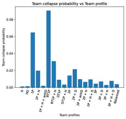
Figure 10. Team collapse probability vs Team profile

Probability of team collapse. In order to empirically estimate the probability of a team collapse for a given team, we count all the times the team collapsed in the simulations and divide by the total number of samples ($1000\times 100=10^{5})$. In these experiments, we consider that $\alpha=1$ (see Dfn. 4); i.e. a team collapses if all its players have choked. In Fig. 10 we show the team-collapse probability for the different team profiles we considered.

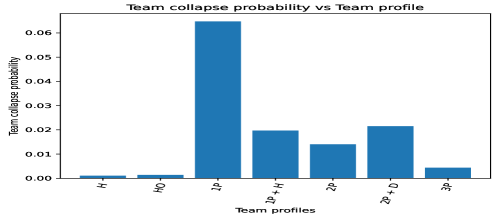
Figure 2. Team collapse probability vs team profile

First, we observe that when all players are completely unaffected by other players (profiles H and HO), then the team rarely collapses. In this case, the only way for a collapse to occur is all players independently under-performing at the same time. In general, adding dependence on the hidden state of the players, i.e., making the players more self-dependent results in a more resilient team.

We also observe that the when there is one pillar in the team (profiles 1Pillar and 1Pillar+H), the team has a single point of failure. That is, when the pillar happens to under-perform, the rest of the players are negatively affected and transition to their lowest mental (hidden) state. Subsequently, these players also under-perform until the performance of the pillar player improves. Naturally, adding more pillars (profiles kPillars, ) makes the team more resilient to collapse since not all pillars under-perform at the same time.

Furthermore, dependence between pillar players (e.g., profile 2Pillars+D) results in less resilient teams. This is because, dependent pillar players have a tendency to under-perform at the same time. Once this happens, the rest of the players transition to hidden state $-1$ and start under-performing.

Finally, we emphasize that a team that doesn’t under-perform isn’t necessarily a good team. Observed performance is measured relatively to the average performance of the team. Thus, a consistently bad team might never under-perform, but still perform poorly relatively to other teams.

3.3. Remarks on team profiles

We summarize here our observations and state some principles we experimentally found to be true and can provide useful insights to experts reasoning about team composition and resilience of teams to collapses.

Remark 1.

(Self-dependence.) Self-dependent players, i.e., players that primarily depend on their own hidden and observed states, improve the resilience of teams.

We say that a player is a pillar if other players heavily depend on him/her, while he/she is self-dependent. For example, a player $i$ is a pillar player if $r_{i}\approx 1$ and $R_{ji}\approx 1,\forall j\in[n]$.

Remark 2.

(Pillars.) More pillars are better than less pillars.

Remark 3.

(Dependence between pillars.) Dependence between pillars makes teams more vulnerable to team collapse.

These observations have several implications in terms of team and roster construction. More specifically, self-dependent players are also typically players that can do several things at a high level. This is in contrast to “specialists” that bring to the team a very well-delineated skillset (e.g., individual defense and three point shooting) and depend on their teammates for other aspects of the game (e.g., shot generation). While lately there are many teams that prioritize the acquisition of specialists who possess specific skillset at an elite level, our observations indicate that having more self-dependent players makes a team more resilient to a possible collapse.

Furthermore, as one might have expected, a team with self-dependent players that can also influence/help their teammates’ performance (i.e., pillar players) is in general more resilient. However, the choice of these pillar players should take into consideration their dependence. According to our third remark, if a team includes pillars that are dependent, the resiliency to team collapse reduces. This dependency can be related to the position the two pillars cover on the team. For instance, if a team’s pillar A is a center and its other pillar B is a guard there can be directional dependency from the B to A, just because B controls the ball more and is the one responsible for distributing it to other players. This dependency does not have to be strong, but its effects can trickle down to the rest of the players. Hence, from a roster-construction perspective, assuming a team already has one pillar, understanding the dependency that will be introduced when adding a second one is crucial. Going back to the example above, the best pillar pairing for player B might be another guard instead of a center.

4. Learning the model

In this section, we describe a learning algorithm. Given the observed states of the players of a team over a period of time, it estimates the parameters of our model and the corresponding hidden states of the players.

Throughout the description we follow the following notation: we use $\mathbf{O}$ to denote the sequence of observations $\mathbf{O}_{1},\cdots,\mathbf{O}_{T}$, where $\mathbf{O}_{t}=(O_{t}^{1},\dots,O_{t}^{n})$ are the observed signals of all entities at time $t$. Accordingly, we use $\mathbf{H}$ to denote the sequence of hidden states $\mathbf{H}_{1},\cdots,\mathbf{H}_{t}$, where $\mathbf{H}_{t}=(H_{t}^{1},\dots,H_{t}^{n})$ are the hidden states of all entities at time $t$. Finally, we use $\mathbf{O}_{1:t}$ to denote $\mathbf{O}_{1},\dots,\mathbf{O}_{t}$. Thus, given $\mathbf{O}$, we want to learn the parameters $\boldsymbol{\Theta}=\{\mathcal{M}^{ij},\mathcal{N}^{i},\mathcal{R},\mathcal{E}^{i}\mid i,j\in[n]\}$ of the model and the sequence of hidden states $\mathbf{H}$.

4.1. Learning the parameters of the model

We learn the parameters of the model by applying the Expectation-Maximization (EM) algorithm. EM alternates between two steps: the expectation step (E-step) and the maximization step (M-step). In our case, these steps are:

E-step: In this step, we need to calculate the expected complete log-likelihood:

(2) $$Q(\boldsymbol{\Theta}\mid\boldsymbol{\Theta}^{\text{old}})=\mathbb{E}_{\mathbf{H}\sim\text{Pr}(\mathbf{H}\mid\mathbf{O},\boldsymbol{\Theta}^{\text{old}})}\left[\log\text{Pr}(\mathbf{H},\mathbf{O}\mid\boldsymbol{\Theta})\right],$$

Usually, we approximate the above expectation by drawing samples from the posterior distribution $\text{Pr}(\mathbf{H}\mid\mathbf{O},\boldsymbol{\Theta})$ and calculating the average of the function.

M-step: In this step, we need to maximize the expected complete log-likelihood w.r.t. the parameters of the model.

EM alternates between the E and the M steps until convergence.

4.1.1. E-step

In the E-step we need to sample from the posterior distribution $\text{Pr}(\mathbf{H}\mid\mathbf{O},\boldsymbol{\Theta})$, assuming that the model parameters $\boldsymbol{\Theta}$ are known. Since it is clear from the context that all probabilities will be conditioned on $\boldsymbol{\Theta}$, we omit the parameters in the condition and write the posterior as $\text{Pr}(\mathbf{H}\mid\mathbf{O})$

The key idea for being able to sample from the posterior is that we need to write $\text{Pr}(\mathbf{H}\mid\mathbf{O})$ as a product where each random variable $\mathbf{H}_{t}$ is only conditioned on observed quantities or on random variables $\mathbf{H}_{t^{\prime}}$ with $t^{\prime}<t$. This is summarized in the following Lemma, which is the main result of this section:

Lemma 0.

It holds that

(3) $$\text{Pr}(\mathbf{H}\mid\mathbf{O})=\prod_{i=1}^{n}\prod_{t=1}^{T}\frac{\text{Pr}(H_{t}^{i}\mid\mathbf{O}_{1:t})}{\text{Pr}(H_{t}^{i}\mid\mathbf{O}_{1:t-1})}\text{Pr}(H_{t}^{i}\mid H_{t-1}^{i},\mathbf{O}_{1:t-1})$$

The proof of the lemma is based on a set of observations and it is quite lengthy, so it is given in Appendix D.1. This lemma allows us to sample $H_{t}^{i}$ from a distribution that is proportional to

$$\frac{\text{Pr}(H_{t}^{i}=h\mid\mathbf{O}_{1:t})\text{Pr}(H_{t}^{i}=h\mid H_{t-1}^{i},\mathbf{O}_{t-1})}{\text{Pr}(H_{t}^{i}=h\mid\mathbf{O}_{1:t-1})},$$

as dictated by Lemma 1.

4.1.2. M-step

In the M-step we want to maximize the the expected complete log-likelihood w.r.t. the parameters of the model. To see how this can be approached we first write the complete likelihood:

$$\text{Pr}(\mathbf{H},\mathbf{O}) =\text{Pr}(\mathbf{H}_{1})\prod_{t=2}^{T}\text{Pr}(\mathbf{H}_{t}\mid\mathbf{H}_{t-1},\mathbf{O}_{t-1})\prod_{t=1}^{T}\text{Pr}(\mathbf{O}_{t}\mid\mathbf{H}_{t})$$

$$=\text{Pr}(\mathbf{H}_{1})\prod_{t=2}^{T}\prod_{i=1}^{n}\text{Pr}(H_{t}^{i}\mid H_{t-1}^{i},\mathbf{O}_{t-1})\prod_{t=1}^{T}\prod_{i=1}^{n}\text{Pr}(O_{t}^{i}\mid H_{t}^{i})$$

Taking the logarithm on both sides we get the complete log-likelihood:

(4) $$\log\text{Pr}(\mathbf{H},\mathbf{O}) =\log\text{Pr}(\mathbf{H}_{1})$$

$$+\sum_{t=2}^{T}\sum_{i=1}^{n}\log\text{Pr}(H_{t}^{i}\mid H_{t-1}^{i},\mathbf{O}_{t-1})$$

$$+\sum_{t=1}^{T}\sum_{i=1}^{n}\log\text{Pr}(O_{t}^{i}\mid H_{t}^{i}).$$

Thus in the M-step we have to solve the following problem:

(5) $$\boldsymbol{\Theta}^{\text{new}}=\operatorname*{arg\,max}_{\boldsymbol{\Theta}}Q(\boldsymbol{\Theta}\mid\boldsymbol{\Theta}^{\text{old}}),$$

where $Q()$ is given by Eq. (2) and the complete log-likelihood is computed by Eq. 4. Note that $Q(\boldsymbol{\Theta}\mid\boldsymbol{\Theta}^{\text{old}})$ is not a concave function in the parameters $\boldsymbol{\Theta}$ and thus finding a global maximum it not easy. Specifically, the problem stems from the terms $\text{Pr}(H_{t}^{i}\mid H_{t-1}^{i},\mathbf{O}_{t-1})$ which contain products of variables. Thus, we opted for a round-robin heuristic algorithm. This heuristic iteratively optimizes one parameter from $\boldsymbol{\Theta}=\{\mathcal{M},\mathcal{N},\mathcal{R}^{i},\mathcal{E}\mid i\in[n]\}$ per iteration, while keeping the other parameters fixed; in all cases fixing all but one of the parameters results in a concave function. Hence, we can use standard convex-optimization tools to optimize for each parameter separately. In practice, we found that 1-2 iterations of the round robin heuristic are adequate.

4.2. Likelihood calculation

Given the model parameters $\boldsymbol{\Theta}$, we can calculate the likelihood of the data $\Pr(\mathbf{O})$, based on the results of the previous section:

(6) $$\log\Pr(\mathbf{O}) =\sum_{t=1}^{T}\sum_{i=1}^{n}\log\Pr(O_{t}^{i}\mid\mathbf{O}_{t-1})$$

(7) $$=\sum_{t=1}^{T}\sum_{i=1}^{n}\log\left[\sum_{h\in\mathcal{H}}\Pr(O_{t}^{i}\mid H_{t}^{i}=h)\Pr(H_{t}^{i}=h\mid\mathbf{O}_{1:t-1})\right].$$

4.3. Decoding the hidden states

In decoding , we find the most likely hidden variables path $\mathbf{H}_{1},\dots,\mathbf{H}_{T}$, given the model parameters $\boldsymbol{\Theta}$ (evaluated by EM) and the observed variables $\mathbf{O}=\mathbf{O}_{1:T}$. Formally, this problem can be expressed as

(8) $$\overline{\mathbf{h}}=\operatorname*{arg\,max}_{\mathbf{h}}\text{Pr}(\mathbf{H}=\mathbf{h}\mid\mathbf{O}).$$

We solve the problem expressed in Eq. (8) via a dynamic-programming algorithm, which is very similar to the Viterbi algorithm used for standard HMMs (Bishop, 2006). To this end, first we decouple the chains

$$\text{Pr}(\mathbf{H}=\mathbf{h}\mid\mathbf{O})=\prod_{i=1}^{n}\text{Pr}(\mathbf{H}^{i}=\mathbf{h}^{i}\mid\mathbf{O}),$$

using the independence of $\mathbf{H}^{i}$ and $\mathbf{H}^{j}$ given $\mathbf{O}$. For each entity $i$, we define $\delta_{i}(t,h)$ to be the probability of the maximum-probability path ending at $H_{t}^{i}=h$; formally:

$$\delta_{i}(t,h)=\max_{h_{1},\dots,h_{t-1}\in\mathcal{H}^{t-1}}$$

$$\text{Pr}(H_{1}^{i}=h_{1},\cdots,H_{t-1}^{i}=h_{t-1},H_{t}^{i}=h\mid O_{1}^{i},\cdots O_{t}^{i}).$$

That is, $\delta_{t}(h)$ is the probability of the most probable path ending at $H_{t}^{i}=h$. Now the values of $\delta_{i}(t,h)$ can be computed using the following dynamic-programming recursion:

$$\delta_{i}(t,h)=\text{Pr}(O_{t}^{i}\mid H_{t}^{i}=h)\times$$

$$\max_{h^{\prime}\in\mathcal{H}}\left(\delta_{i}(t-1,h^{\prime})\text{Pr}(H_{t}^{i}=h\mid H_{t-1}^{i}=h^{\prime},\mathbf{O}_{t-1})\right),$$

$\forall h\in\mathcal{H}$ and $t\in\{1,\ldots,T\}$.

The base case is

$$\delta_{i}(1,h)=\text{Pr}(H_{1}^{i}=h)\text{Pr}(O_{1}^{i}\mid H_{1}^{i}=h),\forall h\in\mathcal{H}.$$

Once all $\delta_{i}(t,h)$ values are computed one can trace back the solutions starting from $\delta_{i}(T,h)$, where $h=\operatorname*{arg\,max}_{h^{\prime}\in\mathcal{H}}\delta_{i}(T,h^{\prime})$.

4.4. Evaluating the learning algorithm on synthetic data

We evaluated our implementation of the EM algorithm on synthetic data as follows. We created a 1Pillar team profile and generated samples that correspond to $T=100$ timesteps. We then ran the EM algorithm and found that it correctly identifies the structure of the team. Figure 3 shows the Negative Evidence Lower Bound (N-ELBO) as a function of the iterations of EM. The figure shows the average and the standard deviation of N-ELBO over $10$ different initializations. As expected, N-ELBO decreases with iterations until it stabilizes to a low value. The negative likelihood of the (best) learned model is $416$, while the negative likelihood of the true model is $417$ (slightly larger). That is, EM finds a model that has even better likelihood than the model used to generate the data.

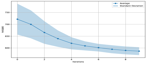
Figure 3. Negative Evidence Lower Bound (N-ELBO) vs iterations of EM; average and standard deviation over 10 random initializations.

Negative Evidence Lower Bound (N-ELBO) vs iterations of EM

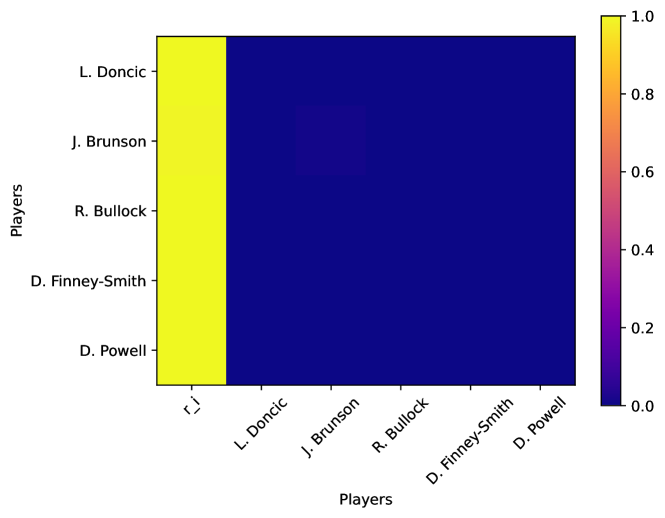
(a) Dallas Mavericks

(b) Cleveland Cavaliers

(c) Boston Celtics

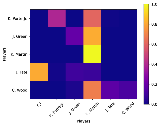
(d) Houston Rockets

Figure 4. Team structure ($\mathcal{R}$) for the Dallas Mavericks, Cleveland Cavaliers, Boston Celtics and Houston Rockets.

5. Real-world experiments

In this section, we validate the practical utility of our model by using it to identify the structure of all NBA teams for the season 2021-2022. We also show how our model can be used to analyze and obtain significant insights for specific games.

5.1. Data

For each NBA team of the 2021-2022 season we selected their starting lineup players. That is, the players that played the most minutes in each position (Point Guard, Shooting Guard, Small Forward, Power Forward, Center).

For our experiment,s we used a Play-by-Play dataset (PBP) that contains a detailed record of events for all NBA games of the season. Using PBP, for each player, we computed his average PIE metric across all quarters (each game has four 12min quarters) of all games. At a high level, the PIE metric of a player for a given time window, captures the percentage of events (points, assists, rebounds, etc) that the player achieved in the given window. Finally, we labeled the performance of every player for every quarter he played as average ($O_{t}^{i}=0$), if his PIE metric was within $\pm\epsilon$ of his average PIE, where $\epsilon=0.05$. If his performance was above this region, we labeled his performance as over-performance $O_{t}^{i}=1$. Accordingly, if his performance was below the average region we labels his performance as under-performance $O_{t}^{i}=-1$. If the player didn’t play in a quarter we used his latest PIE measurement in the game, or if there was no previous measurement we assumed average performance $O_{t}^{i}=1$. We name the resulting dataset NBAseason.

For section 5.4, we created the NBAgames dataset. This dataset contains a few selected games of interest. We divided each of these games into 3 minute time windows so as to have more fine-grained measurements. As before, for each player we computed his average PIE metric in each 3 minute window and labeled his performance.

5.2. Implementation details

In order to apply EM in real data, we created a collection of approximately $10000$ team profiles, i.e., instantiations of our model. These profiles were, to a large extent, informed by our findings in Section 4.4. Then, we found the profile from the collection that best matches each team by calculating the likelihood of the profile. Finally, for each team we ran the EM algorithm initialized with the aforementioned profile.

The implementation of our algorithms, along with the datasets we used in our experiments are publicly available at https://github.com/jasonNikolaou/Team-collapse.git.

5.3. Team structure in NBA teams

Using dataset NBAseason, we applied the EM algorithm to find the maximum-likelihood estimates of the parameters of our model as described in Section 5.2.

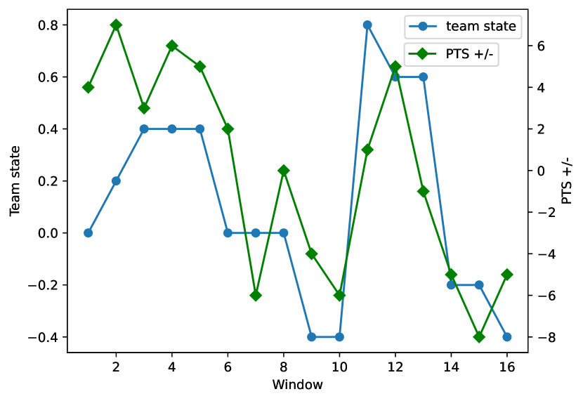
(a) Nets vs Knicks game (16 Feb 2022)

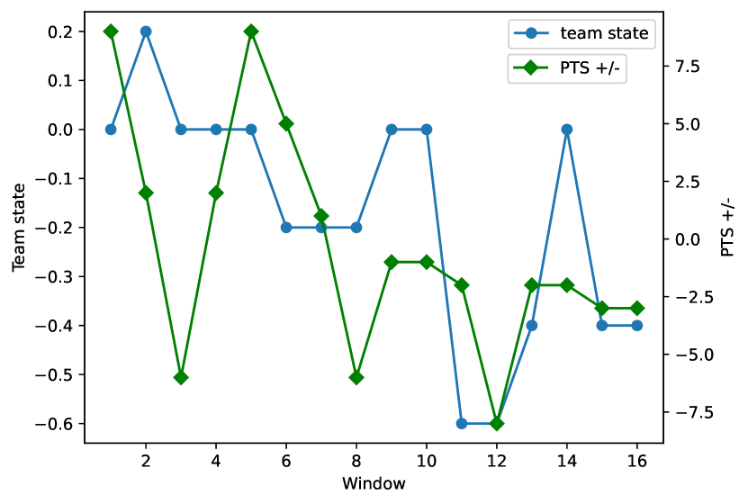
(b) Celtics vs Knicks game (6 Jan 2022)

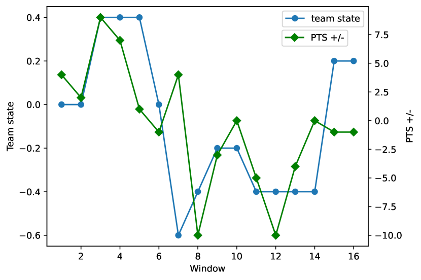
(c) Lakers vs Thunder (27 Oct 2021)

Figure 5. Team (hidden) state and points difference (PTS +/-) per 3 minute window for different games.

Thus, for every one of the 30 NBA teams we obtained an estimate of its team structure $\mathcal{R}$. While of course each team has a different structure, there are two main team-structure types that emerge. In Figure 4 we present four representative teams of these team structures (two for each), while we present the rest of the team structures in Appendix E.1.

The team structures correspond to the matrix $\mathcal{R}$ of the team profile and therefore, they are presented as a $5\times 6$ heatmap. The first column in the heatmap corresponds to the dependency of each row player $i$ to its hidden state (i.e., $r_{i}$), and the rest $5\times 5$ matrix represents the dependency between the hidden state of the row player $i$ and the observed state of the column player $j$.

The first two team structures, shown in Figures 4(a) and 4(b) correspond to the structures of Dallas Mavericks and Cleveland Cavaliers respectively. For the Mavericks, we see that the state of every player is mainly dependent on their own hidden state (first column of the matrix), while they do not depend on their own observations. Simply put, these teams consist of players that typically can showcase “short memory” with respect to their observed performance/state and their state only depends on their own hidden (mental) state. The Cavaliers’ team structure is very similar.

The other two team structures shown in Figures 4(c) and 4(d) correspond to Boston Celtics and Houston Rockets respectively. For Celtics, we see a smaller dependency of their players’ on their own hidden state and a larger dependency for some of them on their observed state. However, there is also a dependency on another player’s observed state (last column in Figure 4(c)). In this particular case , this player is Al Horford, who is the most experienced player on the team and his teammates can be thought of as “feeding off” his observed state/performance. The Rockets team structure (Figure 4(d)) is very similar.

Interestingly, while both the Dallas Mavericks and Boston Celtics have very different structures, they both reached the conference finals and finals respectively. On the other hand, the Houston Rockets, which have structure similar to Boston Celtics, had a record of 20 wins and 62 loses and finished last in the Western conference. This demonstrates that there are many ways to succeed (or fail) in a team sport. The team structure is just one characteristic of a team, among others that create different vulnerabilities and strengths.

5.4. Diving deeper into specific games

For the results we report here, we use the NBAgames dataset described in section 5.1. Using the parameters learned in the previous section, we decode the most probable hidden states of players by applying the decoding algorithm described in Section 4.3.

We now analyze three games in detail. In all these games, one of the teams managed to comeback and win the game despite trailing behind in score for the most part of the game. More analyzed games can be found in the Appendix E.2.

Figure 5 visualizes the hidden team state we obtained from our model over the 3 minute windows, and overlays the actual point differential for the game during these states. In these games, a team was performing well to start the game (Knicks, Celtics and Lakers respectively in the figure order), but later in the game there was a “transition” and they surrendered the lead and ultimately lost the game (i.e., collapsed). As we can see the inferences on the team state made by our model follow closely the point differential, and hence the status, of the game. These results indicate that our model captures the underlying hidden states of the players to a great extent and can explain what one observes at the game.

6. Conclusions

In this paper, we proposed a probabilistic graphical model that allowed us to formalize the dependencies between team players’ hidden/mental states and the observed performance of themselves and their teammates. Then, we used this model to identify, analyze and explain team collapses, i.e., events where a team severely under-performed. We also showed that we can learn the parameters of this model using an EM algorithm. Furthermore, we used our model to analyze real-world team data from NBA games in 2021-22 season. As a result, we found some interesting team structures and identified games where according to our model a team collapsed.

One shortcoming of our model is the assumption that players in the team do not change over time. Considering a dynamic version of the model, where players can get substituted is an interesting direction of future work. In our experiments with real-world data, we relied on the use of the PIE metric to measure the observed performance of players. In the future, we plan to explore other metrics as well as make use of machine learning methods in order to classify the observed performance. Finally, we can potentially use our model to calculate collapse probabilities, as predictors of future collapses. In such a scenario, our model can guide coaching decisions, e.g., substitutions, time-out, etc.

Reproducibility. We make the code and the data we used in our experiments publicly available at https://github.com/jasonNikolaou/Team-collapse.git.

Appendix A Appendix for Section 2

A.1. Proof of Lemma 1

Proof.

$$\sum_{h\in\mathcal{H}}(H_{t}^{i}=h\mid\mathbf{O}_{t-1},H_{t-1}^{i})$$

$$=\sum_{h\in\mathcal{H}}\left(\sum_{j=1}^{n}R_{ij}\text{Infl}(H_{t}^{i}=h\mid O_{t-1}^{j})+R_{i}\text{Infl}(H_{t}^{i}=h\mid H_{t-1}^{i})\right)$$

$$=\sum_{j=1}^{n}R_{ij}\sum_{h\in\mathcal{H}}\text{Infl}(H_{t}^{i}=h\mid O_{t-1}^{j})+R_{i}\sum_{h\in\mathcal{H}}\text{Infl}(H_{t}^{i}=h\mid H_{t-1}^{i})$$

$$=\sum_{j=1}^{n}R_{ij}+R_{i}$$

$$=1.$$

∎

A.2. On the influence matrices

In this section, we answer the following question: why isn’t $\mathcal{M}$ the same as the probability distributions $\text{Pr}(H_{t}^{i}\mid O_{t-1}^{i})$. Consider the following proof by contradiction. Let $n=1$ and $r_{1}=0$, $R_{11}=1$. We define the following parameters:

(9) $$\mathcal{N}=\begin{bmatrix}0&0&1\\ 0&1&0\\ 1&0&0\end{bmatrix},\mathcal{N}=\begin{bmatrix}1&0&0\\ 0&1&0\\ 0&0&1\end{bmatrix},\mathcal{E}=\begin{bmatrix}0.7&0.2&0.1\\ 0.2&0.6&0.2\\ 0.1&0.2&0.7\end{bmatrix},$$

Assume that:

(10) $$\text{Pr}(H_{t}^{i}=h\mid O_{t-1}^{i}=o)=\mathcal{M}[h,o]$$

We have

(11) $$\text{Pr}(H_{t}^{1}=0\mid H_{t-1}^{1}=1,O_{t-1}^{1}=2) =r_{1}\mathcal{N}[1,0]+R_{11}\mathcal{M}[2,0]$$

(12) $$=0+1\times 1$$

(13) $$=1$$

and

(14) $$\text{Pr}(H_{t}^{1}=0\mid H_{t-1}^{1}=1)=\mathcal{N}[1,0]=0.$$

We also have

(15) $$\text{Pr}(H_{t}^{1}=0\mid H_{t-1}^{1}=1) =\sum_{o}\text{Pr}(H_{t}^{1}=0\mid H_{t-1}^{1}=1,O_{t-1}^{1}=o)\text{Pr}(O_{t-1}^{1}=o\mid H_{t-1}^{1}=1)$$

(16) $$\geq\text{Pr}(H_{t}^{1}=0\mid H_{t-1}^{1}=1,O_{t-1}^{1}=2)\text{Pr}(O_{t-1}^{1}=2\mid H_{t-1}^{1}=1)$$

(17) $$\geq 1\times 0.2$$

(18) $$=0.2,$$

which is a contradiction.

In the same way, we can prove that $\mathcal{N}$ isn’t the same as the probability distributions $\text{Pr}(H_{t}^{i}\mid H_{t-1}^{i})$.

Appendix B Appendix for Section 3

B.1. Examples of model parameters used in our experiments

$\mathcal{N}$ instance used in the experiments presented in Section 3:

(19) $$\mathcal{N}=\begin{bmatrix}0.7&0.2&0.1\\ 0.2&0.6&0.2\\ 0.1&0.2&0.7\end{bmatrix}$$

$\mathcal{E}$ instance used in our experiments:

(20) $$\mathcal{E}=\begin{bmatrix}0.8&0.2&0\\ 0.2&0.8&0.2\\ 0&0.2&0.8\end{bmatrix}$$

$\mathcal{M}$ instances used in our experiments in Section 3

(21) $$\mathcal{M}=\begin{bmatrix}0.8&0.2&0\\ 0.2&0.8&0.2\\ 0&0.2&0.8\end{bmatrix},$$

Additional $\mathcal{M}$ instances we considered:

(22) $$\mathcal{M}=\begin{bmatrix}0.9&0.1&0\\ 0.2&0.6&0.2\\ 0.2&0.3&0.5\end{bmatrix}$$

and

(23) $$\mathcal{M}_{\text{anti}}=\begin{bmatrix}0&0.2&0.8\\ 0.1&0.8&0.1\\ 0.8&0.2&0\end{bmatrix}.$$

Additional $\mathcal{R}$ instances we considered In addition to the $\mathcal{R}$ instances we described in Section 3, we also experimented with a few more $\mathcal{R}$ instances. We describe the full set of those instances here:

• $\mathcal{R}_{\text{H}}$: All players depend on their previous hidden state. That is, $r_{i}=1,\forall i\in[n]$ and $R_{ij}=0,\forall i,j\in[n]$. We denote the profile that corresponds to this $\mathcal{R}$ with H.

• $\mathcal{R}_{\text{HO}}$: All players depend only on their previous hidden and observed states. That is, $r_{i}>R_{ii}>0,\forall i\in[n]$ and $R_{ij}=0,\forall i,j\in[n]$. For our experiments we use $r_{i}=0.7$ and $R_{ii}=0.3$, for all $i\in[n]$.

• $\mathcal{R}_{k}$: There are $k$ pillar players $P$ that affect all others; i.e., $r_{i}=R_{ii}=0$ and $R_{ij}=1/|P|$ for all $i\notin P$ and $j\in P$ and $r_{i}=1$ for $i\in P$.

• $\mathcal{R}_{\text{kH}}$: There are $k$ pillar players $P$ that affect all others, but all non-pillar players are also affected by their hidden states. That is, $r_{i}=1$ for all $i\in P$, $r_{i}>0$ for all $i\notin P$ and $R_{ij}=(1-r_{i})1/|P|$ for all $i\notin P$ and $j\in P$. In our experiments we set $r_{i}=0.5$ for all $i\notin P$.

• $\mathcal{R}_{\text{kD}}$: In this case, there are again $k$ pillar players $P$ (as in $\mathcal{R}_{k}$, but this time they depend on each other. That is, for every $i\in P$ $0<r_{i}<1$ and $R_{ij}=(1-r_{i})1/|P|$ for every $i,j\in P$. In our experiments we again set $r_{i}=0.5$.

• $\mathcal{R}_{\text{kDH}}$: This is a combination of $\mathcal{R}_{H}$ and $\mathcal{R}_{kD}$ where all pillar players are set as in $\mathcal{R}_{kD}$ and all non-pillar players are set as in $\mathcal{R}_{\text{kH}}$.

• $\mathcal{R}_{\text{uniform}}$: In this case we assume that for every player $i$, $r_{i}=R_{ij}=1/(n+1)$.

B.2. Team profiles

We create the following extended sets of profiles:

H: $\mathcal{M}$ as above and $\mathcal{R}^{i}=\mathcal{R}_{H}$.

HO. $\mathcal{M}$ as above and $\mathcal{R}^{i}=\mathcal{R}_{\text{HO}}$.

1Pillar (1P). $\mathcal{M}$ as above and $\mathcal{R}^{i}=\mathcal{R}_{\text{1}}$.

1Pillar + Hidden (1P + H). $\mathcal{M}$ as above and $\mathcal{R}^{i}=\mathcal{R}_{\text{1H}}$.

2Pillars (2P). $\mathcal{M}$ as above and $\mathcal{R}^{i}=\mathcal{R}_{\text{2}}$.

2Pillars + Dependence (2P + D). $\mathcal{M}$ as above and $\mathcal{R}^{i}=\mathcal{R}_{\text{2D}}$.

2Pillars + Hidden (2P + H). $\mathcal{M}$ as above and $\mathcal{R}^{i}=\mathcal{R}_{\text{2H}}$.

2Pillars + Hidden + Dependence (2P + H + D). $\mathcal{M}$ as above and $\mathcal{R}^{i}=\mathcal{R}_{\text{2DH}}$.

3Pillars (3P). $\mathcal{M}$ as above and $\mathcal{R}^{i}=\mathcal{R}_{\text{3}}$.

3Pillars + Dependence (3P + D). $\mathcal{M}$ as above and $\mathcal{R}^{i}=\mathcal{R}_{\text{3D}}$.

3Pillars + Hidden (3P + H). $\mathcal{M}$ as above and $\mathcal{R}^{i}=\mathcal{R}_{\text{2H}}$.

3Pillars + Hidden + Dependence (3P + H + D). $\mathcal{M}$ as above and $\mathcal{R}^{i}=\mathcal{R}_{\text{2DH}}$.

Uniform. Players equally depend on their hidden states and other players, i.e. $R_{i}=1/6,R_{ij}=1/6,\forall i,j\in[n]$.

1Pillar Bad Teammate (BT1P). Same as the 1Pillar profile, but we change the $\mathcal{M}$ matrix to the following:

(24) $$\mathcal{M}=\begin{bmatrix}0.9&0.1&0\\ 0.2&0.6&0.2\\ 0.2&0.3&0.5\end{bmatrix}.$$

We are trying to capture a pillar who has significantly negative impact when his/her observed state is $-1$ (i.e. below-average performance), and weakly positive impact when their observed state is $1$ (i.e. above-average performance).

1Pillar Bad Teammate + Hidden (BT1P). Same as the 1Pillar + Hidden profile, but with the $\mathcal{M}$ matrix of the BT1P profile.

1Pillar Great Teammate (GT1S). Same as the 1Pillar profile, but we change the $\mathbf{M}$ matrix to the following:

(25) $$\mathcal{M}=\begin{bmatrix}0.5&0.3&0.2\\ 0.1&0.8&0.1\\ 0&0.1&0.9\end{bmatrix}.$$

This profile captures a pillar who has significantly positive impact when their observed state is $1$ (i.e. above-average performance), and weakly negative impact when their observed state is $-1$ (i.e. below-average performance).

1Pillar Great Teammate + Hidden (GT1P). Same as the 1Pillar + Hidden profile, but with the $\mathcal{M}$ matrix of the 1-Pillar Great Teammate profile.

Finally, we create two profiles to capture anti-dependence. That is, when one player’s performance improves, another player’s performance drops. We define the anti-dependence $\mathcal{M}$ matrix as:

(26) $$\mathcal{M}^{\text{antiD}}=\begin{bmatrix}0&0.2&0.8\\ 0.1&0.8&0.1\\ 0.8&0.2&0\end{bmatrix}.$$

1Pillar + anti-Dependence (1Pillar + antiD). Same as the 1Pillar profile, but we change the $\mathcal{M}$ to $\mathcal{M}^{\text{antiD}}$.

2Pillars + anti-Dependence (2Pillars + antiD). Same as the 2Pillar profile, but we change the $\mathcal{M}$ matrix of both pillars to $\mathcal{M}^{\text{antiD}}$. In this way, the two pillars are anti-dependent on each other. Note that the pillars don’t depend at all on non-pillar players.

B.3. Team state over time

In order to better understand our models we experiment with the 19 profiles described in Appendix B.2. For each profile we types of teams and then run $1000$ simulations. Each simulation consists of $100$ samples. We assume that every player $i\in[n]$ starts from hidden state $H_{1}^{i}=0$. In our experiments, we use 19 different team profiles, which correspond to different combinations of $\mathcal{R}$ and $\mathcal{M}$ pairs.

We define the hidden team state (resp. observed team state) at each timestep as the average of the hidden (resp. observed) states of the individuals in the team at this timestep; values close to $0$ correspond to average team performance, values close to $-1$ (resp. $1$) correspond to an under-performing (resp. over-performing) team. The team (hidden) state of the different teams over time is shown in Figures 6 -  9. In these plots the thick green region corresponds to the 25-th and 75-th percentiles of the team state across simulations. The light green region corresponds to the min and max values of the team state across simulations.

Depending on the team profile, the thick green band might vary its width. Teams with a narrow green band, are more stable, since in $50\%$ of the time they are close to their average mental state. Furthermore, its worth noticing that for some profiles the green band is shifted either upwards (e.g. GT1P) or downwards (e.g BT1P). This shift reveals an inclination of a team towards higher (or lower) mental states.

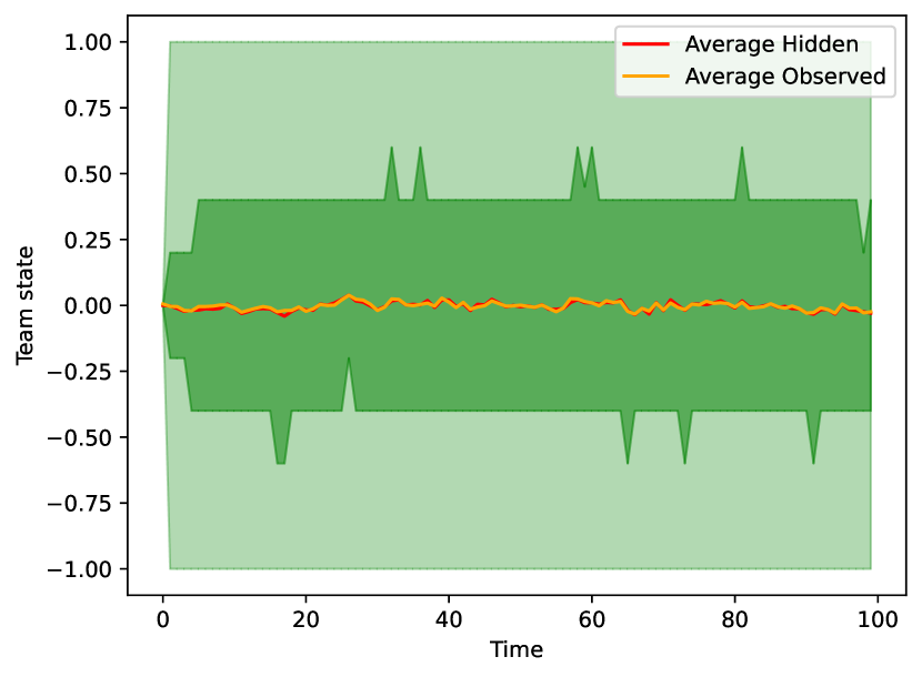
(a) 1Pillar

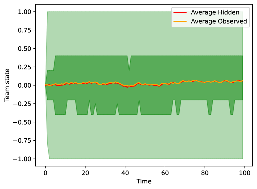
(b) 1Pillar + H

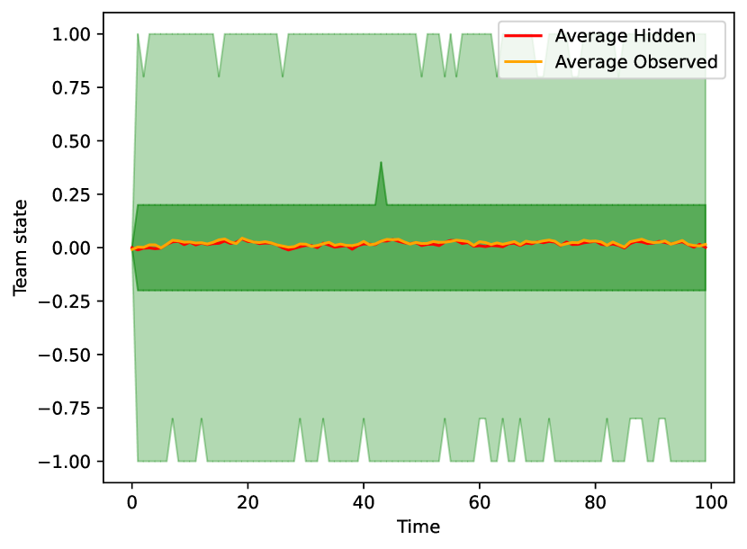
(c) 1Pillar + H + antiD

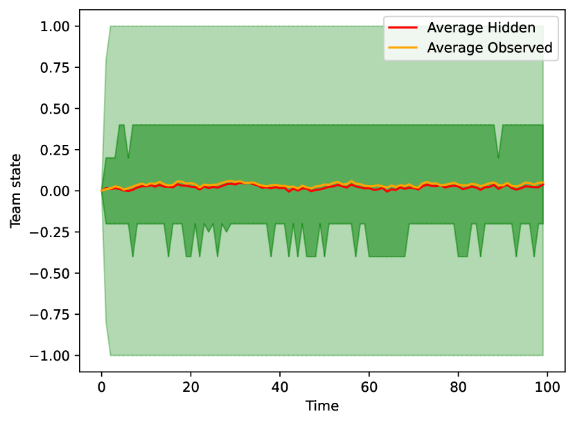
(d) 2Pillars

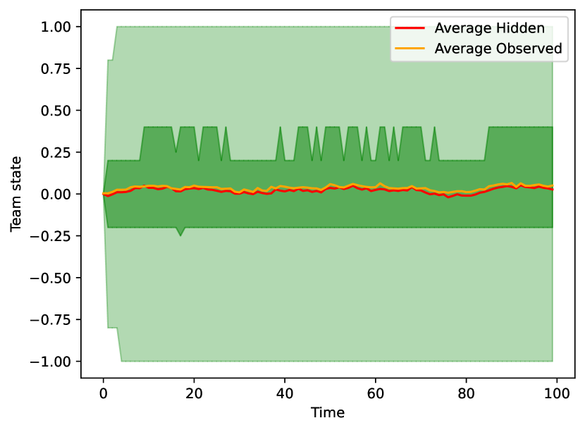
(e) 2Pillars + H

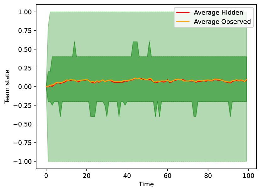
(f) 2Pillars + D

Figure 6. Average hidden and observed states for each team profile

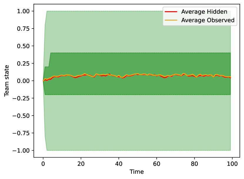
(a) 2Pillars + H + D

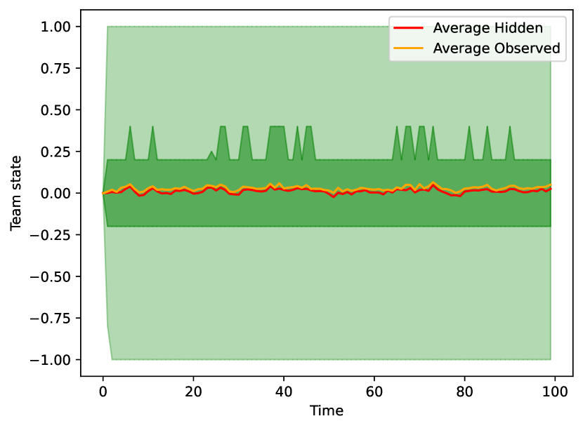
(b) 2Pillars + antiD

(c) 3Pillars

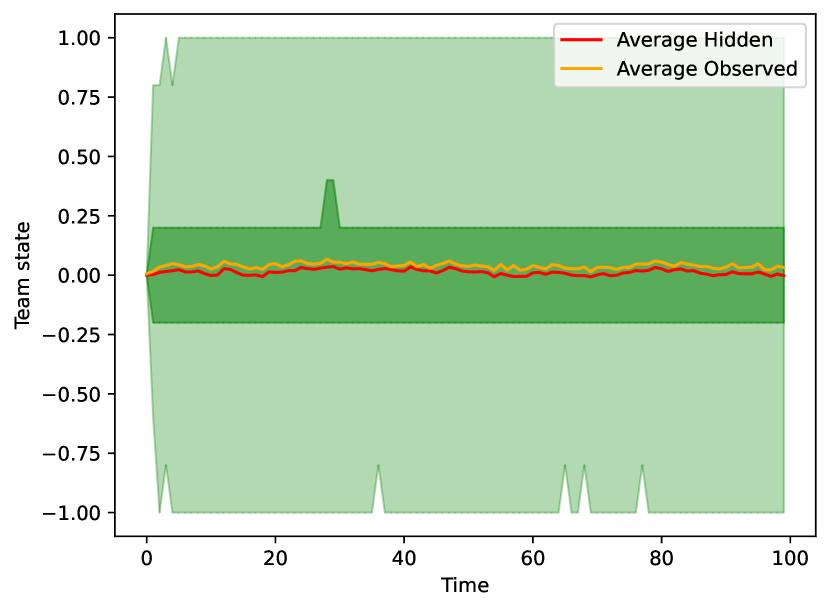
(d) 3Pillars + H

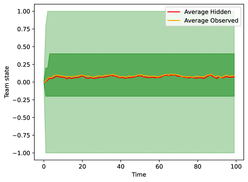
(e) 3Pillars + D

(f) 3Pillars + H + D

Figure 7. Average hidden and observed states for each team profile

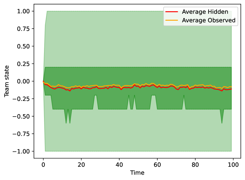
(a) 1Pillar Bad Teammate (BT1P)

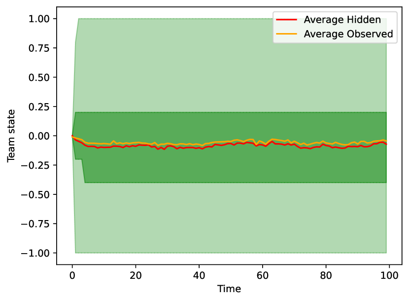
(b) 1Pillar Bad Teammate (BT1P) + H

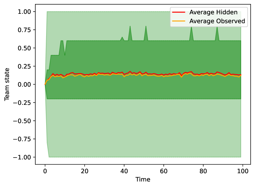
(c) 1Pillar Great Teammate (GT1T)

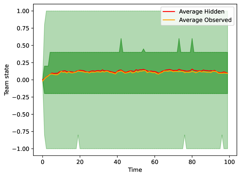
(d) 1Pillar Great Teammate (GT1T) + H

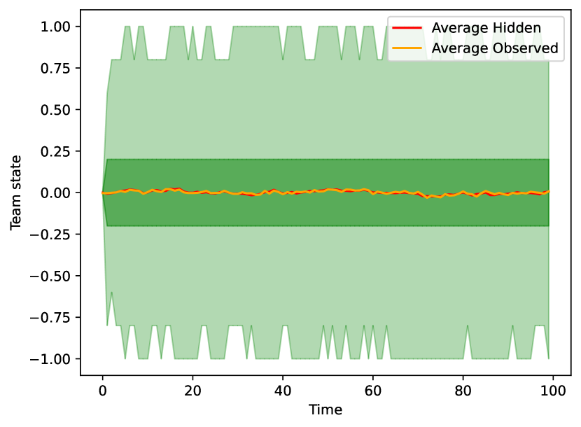
(e) H

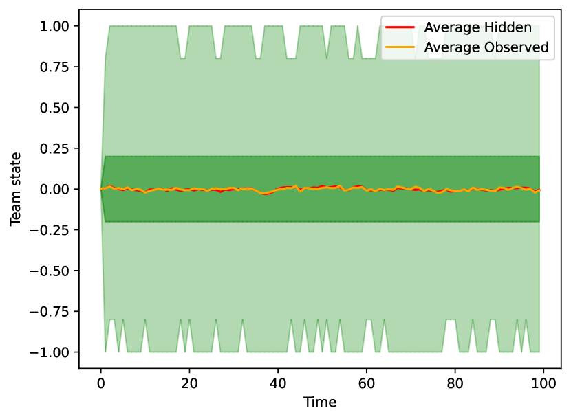
(f) HO

Figure 8. Average hidden and observed states for each team profile

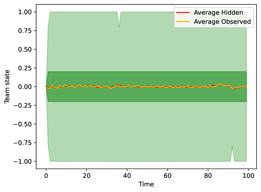
(a) Balanced

Figure 9. Average hidden and observed team states for each team profile; average is taken over different simulations

B.4. Team collapse probability vs Team profile

team collapse probability vs team profile

B.5. Maximum and average time in collapse state

(a) Maximum time in team collapse

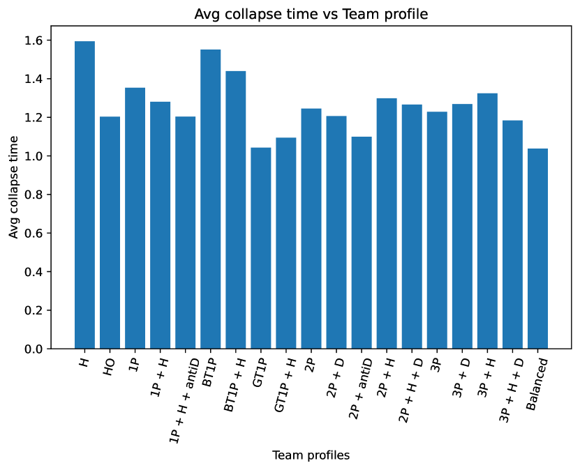
(b) Average time in collapse

Figure 11. Maximum and average time team team collapse

In figure 11 (a), we observe that the more pillars a team has, the longer the maximum window of team collapse is. In general adding self-dependence, i.e. dependence on the hidden states, doesn’t always make the team more resilient. However, adding self-dependence in the 3Pillars profile resulted in higher maximum collapse time. Moreover, we observe that having a Great Teammate player on whom all other players depend (1Pillar Great Teammate (GT1T) profile), significantly reduces the length of the maximum time collapse window. This is because when the pillar player under-performs, he/she only mildly affects non-pillar players. On the contrary, if the pillar player over-performs, non-pillar players are greatly affected in a positive way.

In Figure 11 (b), we observe that the average collapse time doesn’t significantly vary among team profiles. That said, it is clear that when the players only depend on their hidden state, i.e.H profile, the average duration of the collapse is longer. This is because, in the rare case that all players choke, it is very difficult to get out of the choke. For example, this is not the case for the 1Pillar profile. When the pillar of the team chokes, non-pillar players are likely to choke. But, once the pillar player gets out of the choke, non-pillar players are likely to do the same.

Appendix C Independence

In graphical models, independence between random variables is defined using the concept of $d$-separation. For a definition and analysis of $d$-separation see (Koller and Friedman, 2009). We use $X\perp Y\mid Z$ to denote that $X$ is independent of $Y$ given $Z$. In our proofs we used the following independence relationships:

• $H_{t}^{i}\perp H_{t}^{j}\mid\mathbf{O}_{1:t}$

• $O_{t}^{i}\perp\mathbf{O}_{t}^{-i}\mid H_{t}^{i}$

• $H_{t}^{i}\perp\mathbf{O}_{t}^{-i}\mid\mathbf{O}_{1:t-1}$

• $O_{t}^{i}\perp\mathbf{O}_{t}^{1:t-1}\mid H_{t}^{i}$

• $(H_{t}^{i},O_{t}^{i})\perp(H_{t}^{j},O_{t}^{j})\mid\mathbf{O}_{1:t-1}$

• $\mathbf{H}^{i}\perp\mathbf{H}^{j}\mid\mathbf{O}$

Apart from checking the above relationships using the rules of $d$-separation, we also checked them using independence checker programs that are freely available online.

Appendix D Appendix for Section 4

D.1. Expectation step

Calculating the posterior. Using the definition of conditional probability we have that the posterior can be written as

(27) $$\text{Pr}(\mathbf{H}\mid\mathbf{O})=\frac{\text{Pr}(\mathbf{H},\mathbf{O})}{\text{Pr}(\mathbf{O})}.$$

Now, using the structure of the graphical model (see Fig. 1), we can decompose the joint probability of the variables as a product of probabilities where each variable is conditioned on its parent nodes (Koller and Friedman, 2009). Thus, we have

(28) $$\text{Pr}(\mathbf{H},\mathbf{O})=\text{Pr}(\mathbf{H}_{1})\prod_{t=1}^{T}\prod_{i=1}^{n}\text{Pr}(O_{t}^{i}\mid H_{t}^{i})\prod_{t=2}^{T}\prod_{i=2}^{n}\text{Pr}(H_{t}^{i}\mid H_{t-1}^{i},\mathbf{O}_{t-1})$$

Thus, the difficulty of sampling from the posterior stems from the denominator $\text{Pr}(\mathbf{O})$ which can be written as

(29) $$\text{Pr}(\mathbf{O})=\text{Pr}(\mathbf{O}_{1})\prod\text{Pr}(\mathbf{O}_{t}\mid\mathbf{O}_{1:t-1}).$$

In general, calculating $\text{Pr}(\mathbf{O})$ is difficult, however in our model it can be done efficiently by calculating $\text{Pr}(\mathbf{O}_{t}\mid\mathbf{O}_{1:t-1})$. We do this as follows. First, we define the forward parameters

(30) $$\text{Pr}({\mathbf{H}_{t}\mid\mathbf{O}_{1:t}})=\prod_{i=1}^{n}\text{Pr}(H_{t}^{i}\mid\mathbf{O}_{1:t}),$$

where we used the independence of $H_{t}^{i}$ and $H_{t}^{j}$ given $\mathbf{O}_{1:t}$. We now calculate $\text{Pr}(H_{t}^{i}|\mathbf{O}_{1:t-1})$.

(31) $$\text{Pr}(H_{t}^{i}\mid\mathbf{O}_{1:t}) =\text{Pr}(H_{t}^{i}\mid\mathbf{O}_{1:t-1},\mathbf{O}_{t})$$

(32) $$=\frac{\text{Pr}(\mathbf{O}_{t}\mid H_{t}^{i},\mathbf{O}_{1:t-1})\text{Pr}(H_{t}^{i}\mid\mathbf{O}_{1:t-1})}{\text{Pr}(\mathbf{O}_{t}\mid\mathbf{O}_{1:t-1})}$$

(33) $$=\frac{\text{Pr}(\mathbf{O}_{t}^{-i}\mid\mathbf{O}_{1:t-1})\text{Pr}(O_{t}^{i}\mid H_{t}^{i},\mathbf{O}_{1:t-1})\text{Pr}(H_{t}^{i}\mid\mathbf{O}_{1:t-1})}{\text{Pr}(O_{t}^{i}\mid\mathbf{O}_{1:t-1})\text{Pr}(\mathbf{O}_{t}^{-i}\mid\mathbf{O}_{1:t-1})}$$

(34) $$=\frac{\text{Pr}(O_{t}^{i}\mid H_{t}^{i})\text{Pr}(H_{t}^{i}\mid\mathbf{O}_{1:t-1})}{\text{Pr}(O_{t}^{i}\mid\mathbf{O}_{1:t-1})},$$

where in the second equation we used Bayes’ rule, in the third equation we used the independence between $O_{t}^{i}$ and $\mathbf{O}_{t}^{-i}$ given $\mathbf{O}_{1:t-1}$ and the independence of $\mathbf{O}_{t}^{-i}$ and $H_{t}^{i}$ given $\mathbf{O}_{1:t-1}$, and in the last equation we used the independence of $O_{t}^{i}$ and $\mathbf{O}_{1:t-1}$ given $H_{t}^{i}$. Furthermore, we have

(35) $$\text{Pr}(H_{t}^{i}\mid\mathbf{O}_{1:t-1})=\sum_{h\in\mathcal{H}}\text{Pr}(H_{t}^{i}\mid H_{t-1}^{i}=h,\mathbf{O}_{1:t-1})\text{Pr}(H_{t-1}^{i}\mid\mathbf{O}_{1:t-1}),$$

where $\text{Pr}(H_{t-1}^{i}\mid\mathbf{O}_{1:t-1})$ can be calculated recursively.

We also have

(36) $$\text{Pr}(\mathbf{H}_{t},\mathbf{O}_{t}\mid\mathbf{O}_{1:t-1}) =\prod_{i=1}^{n}\text{Pr}(H_{t}^{i},O_{t}^{i}\mid\mathbf{O}_{1:t-1})$$

(37) $$=\prod_{i=1}^{n}\text{Pr}(O_{t}^{i}\mid H_{t}^{i},\mathbf{O}_{1:t-1})\text{Pr}(H_{t}^{i}\mid\mathbf{O}_{1:t-1})$$

(38) $$=\prod_{i=1}^{n}\text{Pr}(O_{t}^{i}\mid H_{t}^{i})\text{Pr}(H_{t}^{i}\mid\mathbf{O}_{1:t-1}),$$

where in the first equation we used the independence of $(H_{t}^{i},O_{t}^{i})$ and $(H_{t}^{j},O_{t}^{j})$ given $\mathbf{O}_{1:t-1}$, and in the third equation we used the independence of $O_{t}^{i}$ and $\mathbf{O}_{1:t-1}$ given $H_{t}^{i}$.

Moreover, we have

(39) $$\text{Pr}(\mathbf{H}_{t}\mid\mathbf{O}_{1:t}) =\frac{\text{Pr}(\mathbf{H}_{t},\mathbf{O}_{t}\mid\mathbf{O}_{1:t-1})}{\text{Pr}(\mathbf{O}_{t}\mid\mathbf{O}_{1:t-1})}$$

Having computed $\text{Pr}(\mathbf{H}_{t}\mid\mathbf{O}_{1:t})$ and $\text{Pr}(\mathbf{H}_{t},\mathbf{O}_{t}\mid\mathbf{O}_{1:t-1})$ we can calculate $\text{Pr}(\mathbf{O}_{t}\mid\mathbf{O}_{1:t-1})$ using the above equation. Thus, we can compute $\text{Pr}(\mathbf{O})$ and the posterior distribution.

The E-step concludes by defining $Q(\boldsymbol{\Theta}\mid\boldsymbol{\Theta}^{\text{old}})$ as the expected value of the log likelihood function of $\boldsymbol{\Theta}$, with respect to the current conditional distribution of $\mathbf{H}$ given $\mathbf{O}$ and the current estimates of the parameters:

(40) $$Q(\boldsymbol{\Theta}\mid\boldsymbol{\Theta}^{\text{old}})=\mathbb{E}_{\mathbf{H}\sim\text{Pr}(\mathbf{H}\mid\mathbf{O},\boldsymbol{\Theta}^{\text{old}})}\left[\log\text{Pr}(\mathbf{H},\mathbf{O}\mid\boldsymbol{\Theta})\right]$$

In practice, we estimate the expectation by drawing samples from the posterior distribution $\text{Pr}(\mathbf{H}\mid\mathbf{O},\boldsymbol{\Theta}^{\text{old}})$, and using the empirical mean. To this end, we next show how to generate samples from the posterior distribution.

Sampling from the posterior. We are now ready to prove Lemma 1 that allows us to decompose the posterior distribution into products of simpler distributions.

Proof.

First, based on the previous analysis, we have

(41) $$\text{Pr}(\mathbf{O}_{t}\mid\mathbf{O}_{1:t-1}) =\frac{\text{Pr}(\mathbf{H}_{t},\mathbf{O}_{t}\mid\mathbf{O}_{1:t-1})}{\text{Pr}(\mathbf{H}_{t}\mid\mathbf{O}_{1:t})}$$

(42) $$=\prod_{i=1}^{n}\frac{\text{Pr}(H_{t}^{i},O_{t}^{i}\mid\mathbf{O}_{1:t-1})}{\text{Pr}(H_{t}^{i}\mid\mathbf{O}_{1:t})}$$

(43) $$=\prod_{i=1}^{n}\frac{\text{Pr}(O_{t}^{i}\mid H_{t}^{i})\text{Pr}(H_{t}^{i}\mid\mathbf{O}_{1:t-1})}{\text{Pr}(H_{t}^{i}\mid\mathbf{O}_{1:t})}.$$

Hence, the evidence becomes

(44) $$\text{Pr}(\mathbf{O}) =\prod_{t=1}^{T}\text{Pr}(\mathbf{O}_{t}\mid\mathbf{O}_{1:t-1})$$

(45) $$=\prod_{t=1}^{T}\prod_{i=1}^{n}\frac{\text{Pr}(H_{t}^{i},O_{t}^{i}\mid\mathbf{O}_{1:t-1})}{\text{Pr}(H_{t}^{i}\mid\mathbf{O}_{1:t})}$$

(46) $$=\prod_{t=1}^{T}\prod_{i=1}^{n}\frac{\text{Pr}(O_{t}^{i}\mid H_{t}^{i})\text{Pr}(H_{t}^{i}\mid\mathbf{O}_{1:t-1})}{\text{Pr}(H_{t}^{i}\mid\mathbf{O}_{1:t})}.$$

Finally, substituting the above into the definition of the posterior distribution and combining with the joint distribution, we have

(47) $$Pr(\mathbf{H}\mid\mathbf{O}) =\frac{\text{Pr}(\mathbf{H},\mathbf{O})}{\text{Pr}(\mathbf{O})}$$

(48) $$=\prod_{t=1}^{T}\prod_{i=1}^{n}\frac{\text{Pr}(O_{t}^{i}\mid H_{t}^{i})\text{Pr}(H_{t}^{i}\mid H_{t-1}^{i},\mathbf{O}_{t-1})}{\text{Pr}(O_{t}^{i}\mid H_{t}^{i})\text{Pr}(H_{t}^{i}\mid\mathbf{O}_{1:t-1})/\text{Pr}(H_{t}^{i}\mid\mathbf{O}_{1:t})}$$

(49) $$=\prod_{t=1}^{T}\prod_{i=1}^{n}\frac{\text{Pr}(H_{t}^{i}\mid\mathbf{O}_{1:t})\text{Pr}(H_{t}^{i}\mid H_{t-1}^{i},\mathbf{O}_{t-1})}{\text{Pr}(H_{t}^{i}\mid\mathbf{O}_{1:t-1})}$$

. ∎

Thus, we sample $H_{t}^{i}$ from a propability distribution that is proportional to

(50) $$\frac{\text{Pr}(H_{t}^{i}=h\mid\mathbf{O}_{1:t})\text{Pr}(H_{t}^{i}=h\mid H_{t-1}^{i},\mathbf{O}_{t-1})}{\text{Pr}(H_{t}^{i}=h\mid\mathbf{O}_{1:t-1})}.$$

Appendix E Real-world experiments

E.1. Team structures

Figure 12 presents the structure matrix for all 30 NBA teams in our dataset. As discussed in Section 5 there are two main profiles and each team can be thought of as falling closer to one of them. For example the Cleveland Cavaliers, fall closer to the profile we saw for the Dallas Mavericks, but with the added difference that two of their players also depend slightly to their own observed state (not only their hidden state). At the same time, Houston Rockets are closer to the profile we saw for the Boston Celtics, where the observed state of Martin seems to impact the state of his teammates.

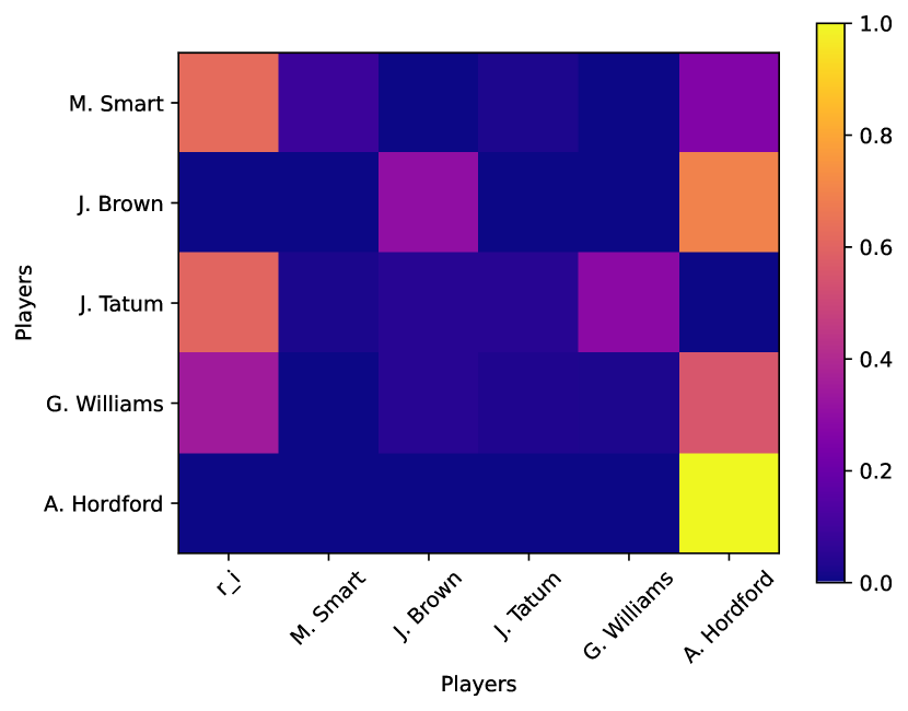
(a) Boston Celtics

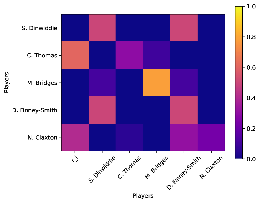
(b) Brooklyn Nets

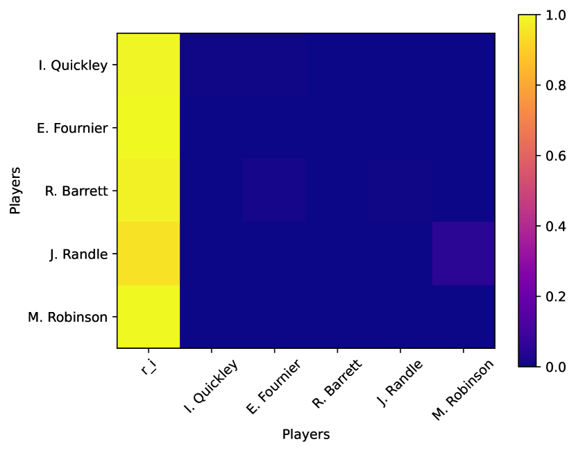
(c) New York Knicks

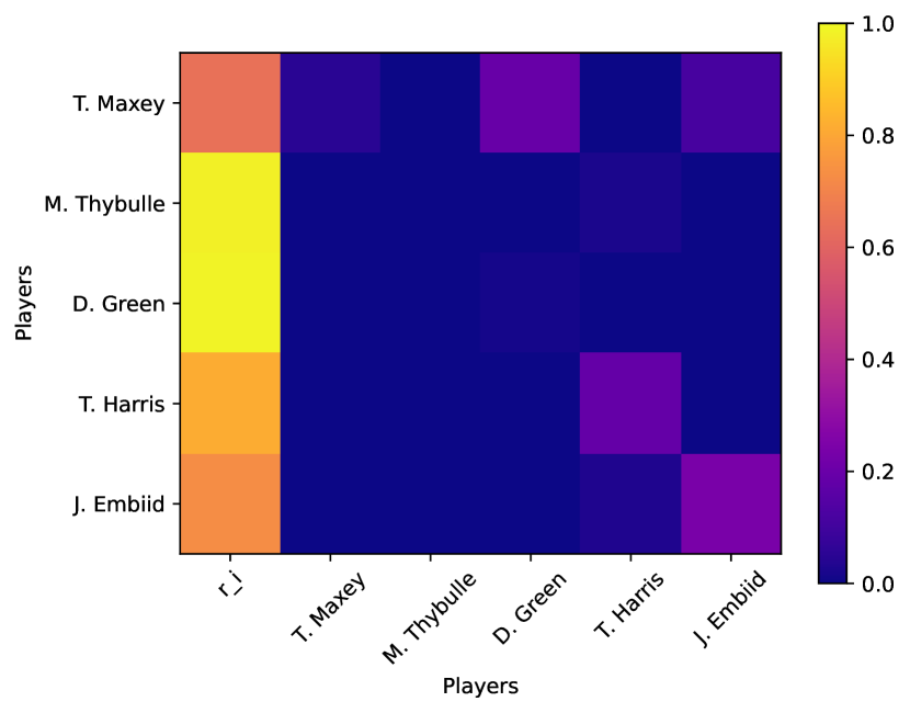
(d) Philadelphia 76ers

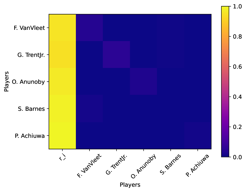
(e) Toronto Raptors

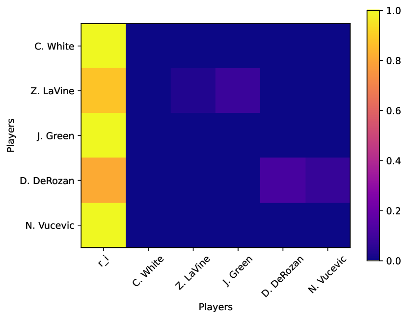
(f) Chicago Bulls

Figure 12. Team structure $\mathcal{R}$

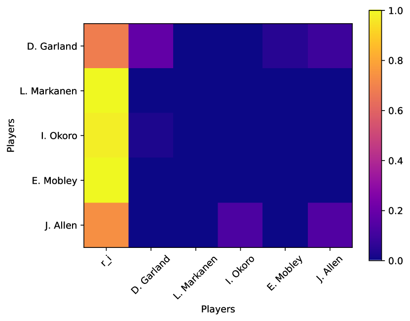
(a) Cleveland Cavaliers

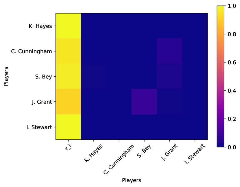
(b) Detroit Pistons

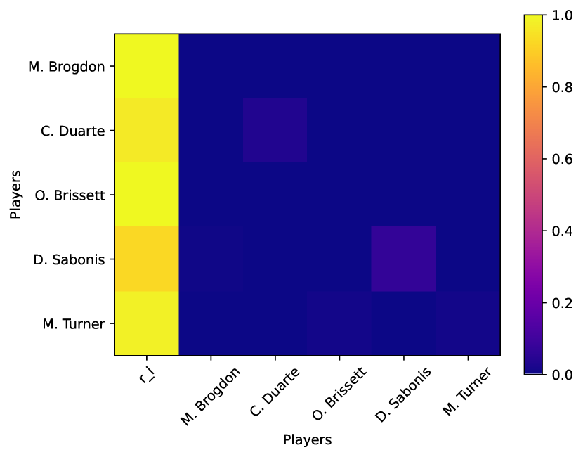
(c) Indiana Pacers

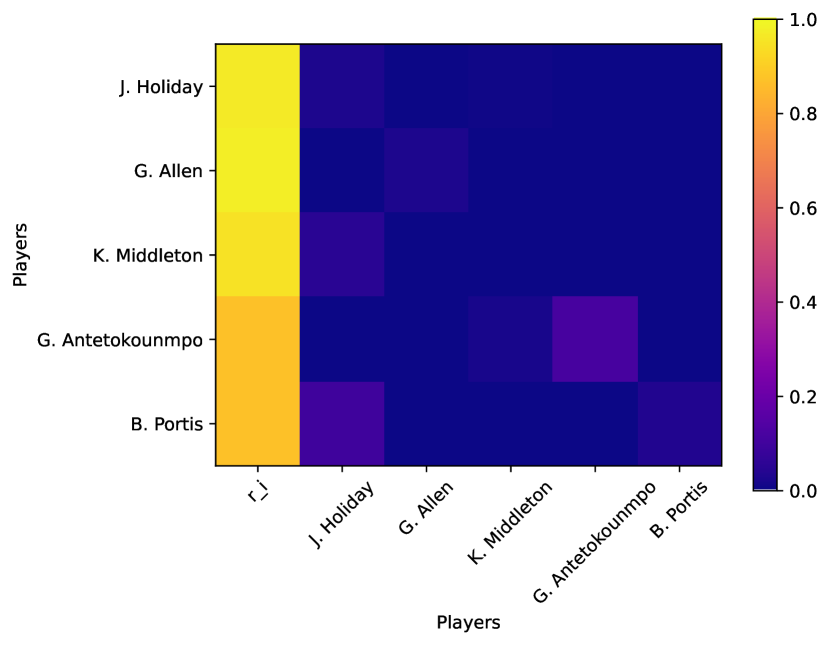
(d) Milwaukee Bucks

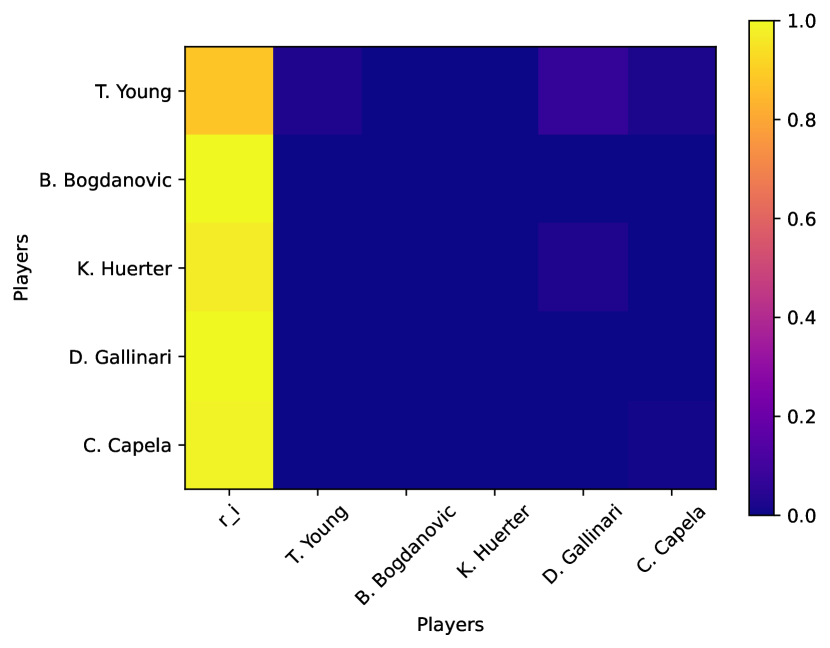
(e) Atlanta Hawks

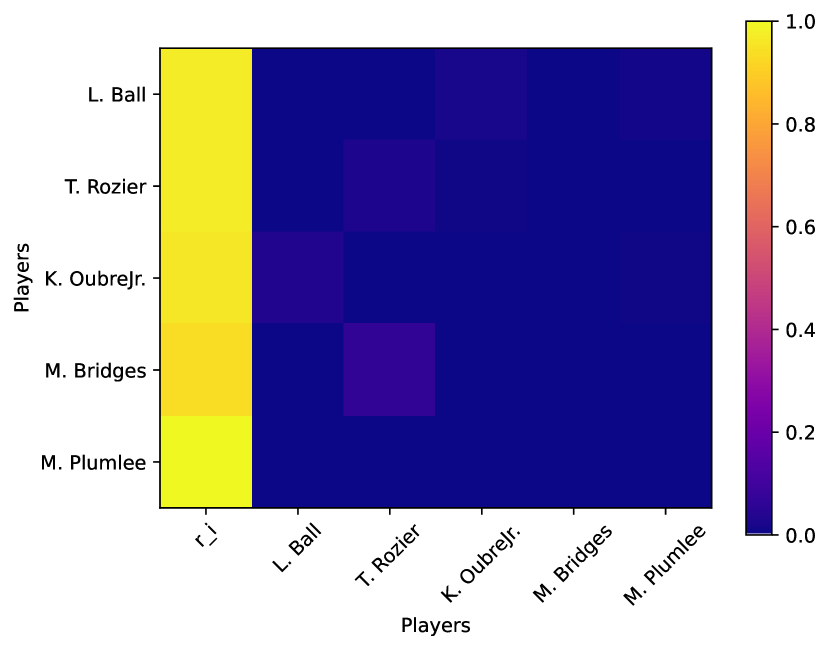
(f) Charlotte Hornets

Figure 13. Team structure $\mathcal{R}$

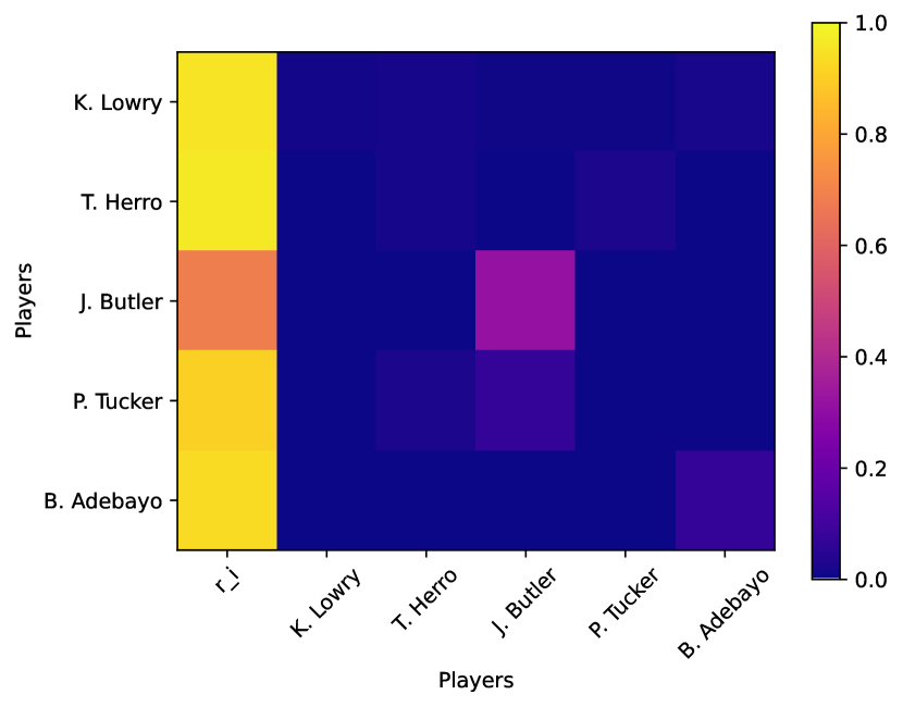
(a) Miami Heat

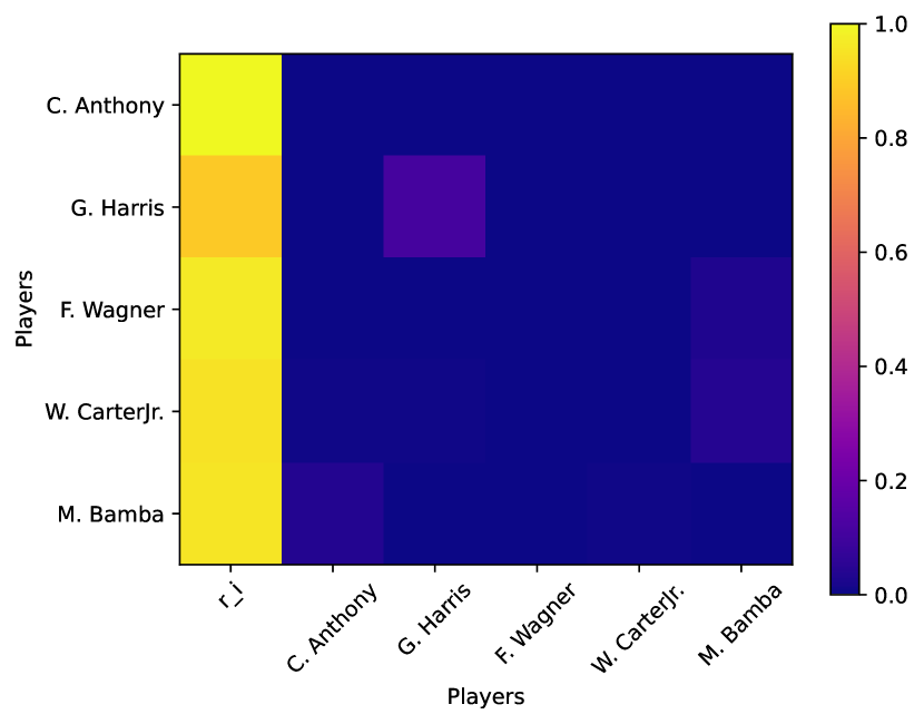
(b) Orlando Magic

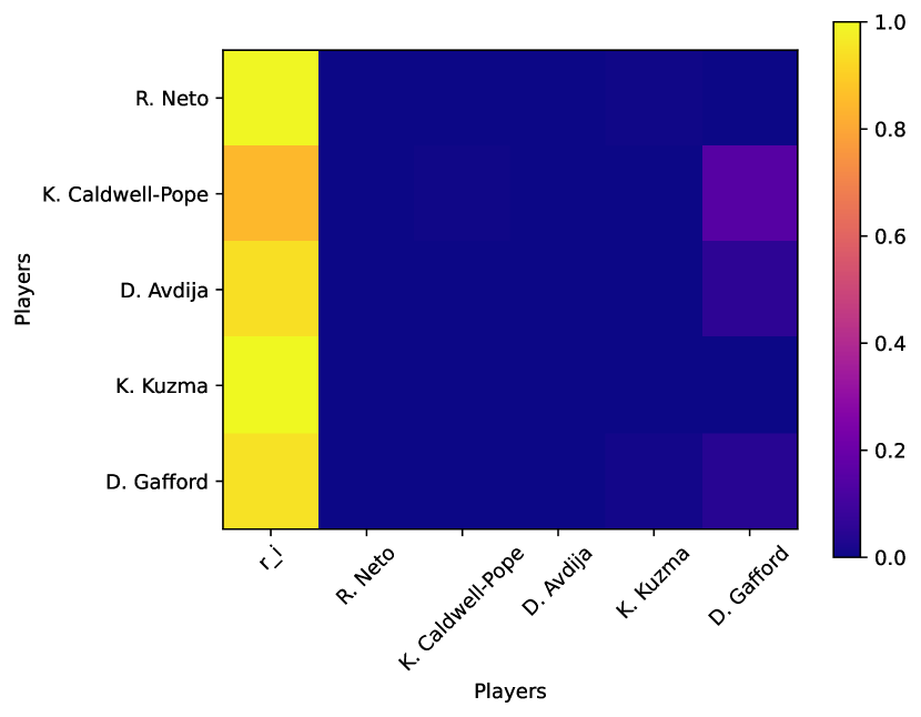
(c) Washington Wizards

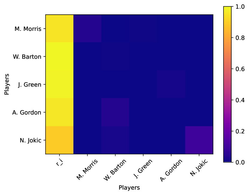
(d) Denver Nuggets

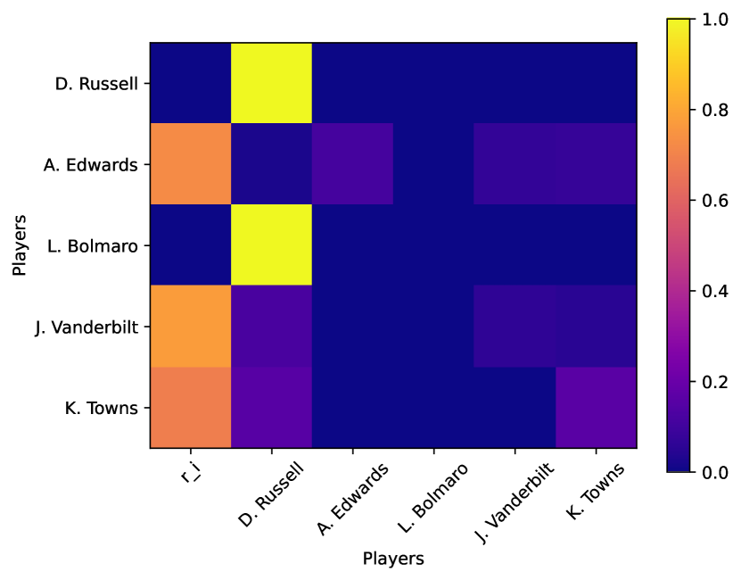
(e) Minnesota Timberwolves

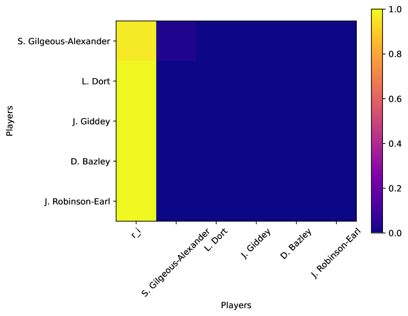
(f) Oklahoma City Thunder

Figure 14. Team structure $\mathcal{R}$

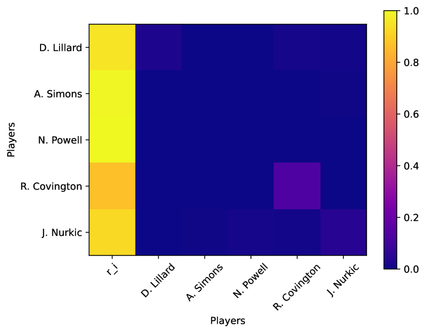
(a) Portland Trail Blazers

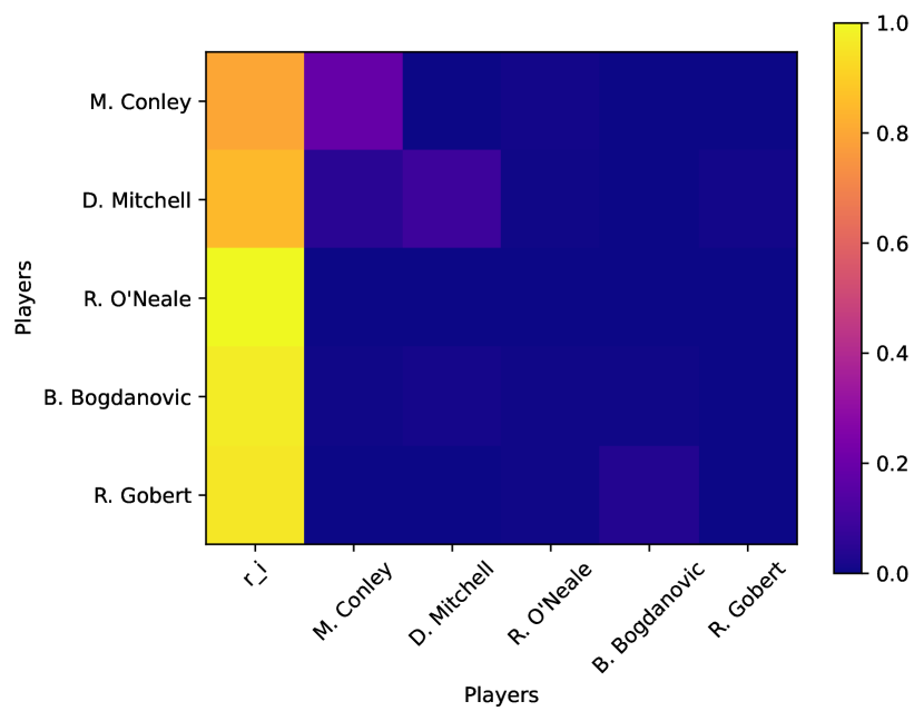
(b) Utah Jazz

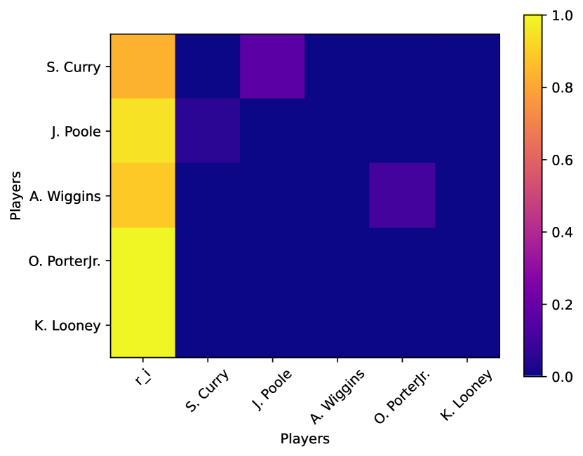
(c) Golden State Warriors

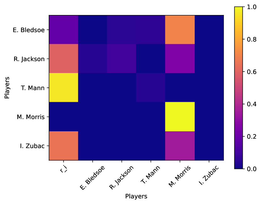
(d) LA Clippers

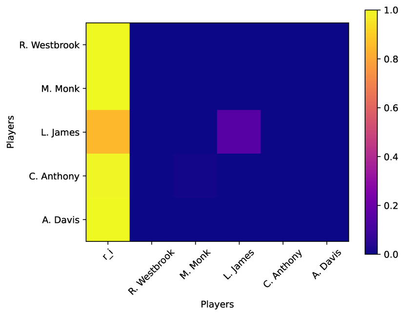
(e) Los Angeles Lakers

(f) Phoenix Suns

Figure 15. Team structure $\mathcal{R}$

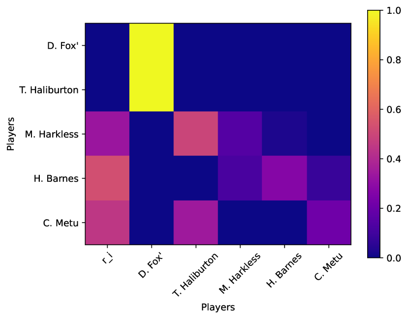
(a) Sacramento Kings

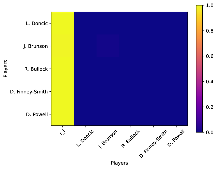
(b) Dallas Mavericks

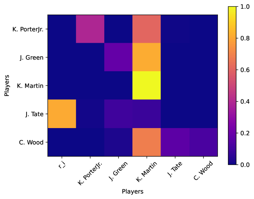
(c) Houston Rockets

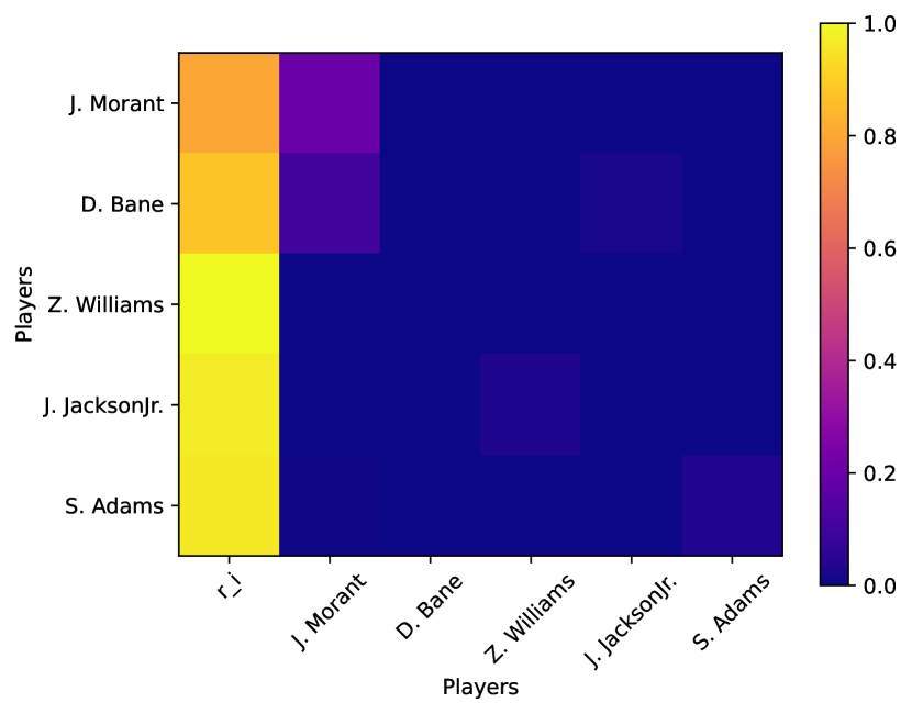
(d) Memphis Grizzlies

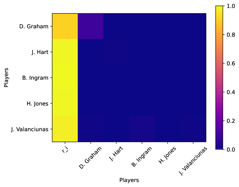
(e) New Orleans Pelicans

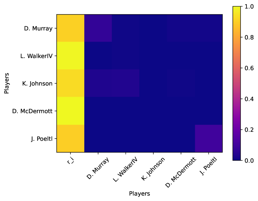
(f) San Antonio Spurs

Figure 16. Team structure $\mathcal{R}$

E.2. Additional examples of specific games

The following figure provides some additional examples of games with the inferred from our model team state. As we can see here also, the team states inferred from our model follows closely in the vast majority of the cases the observed score differential at the game. All in all, the expressivity of our model is very good and can explain well the observed output of the game.

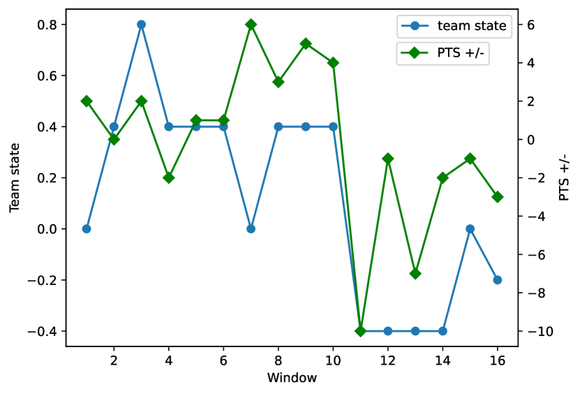
(a) Denver Nuggets vs Los Angeles Lakers(11 Jan 2022)

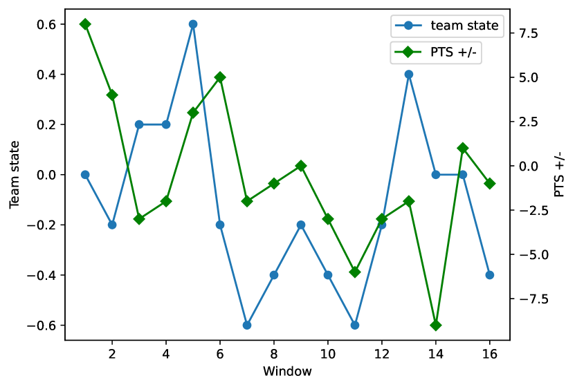
(b) Dallas Mavericks vs Golden State Warriors (20 May 2022)

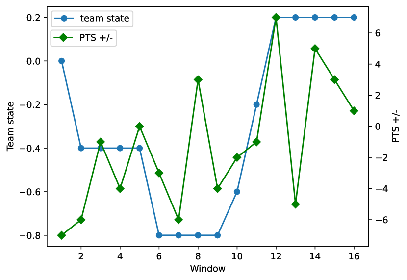
(c) Miami Heat vs Boston Celtics (23 May 2022)

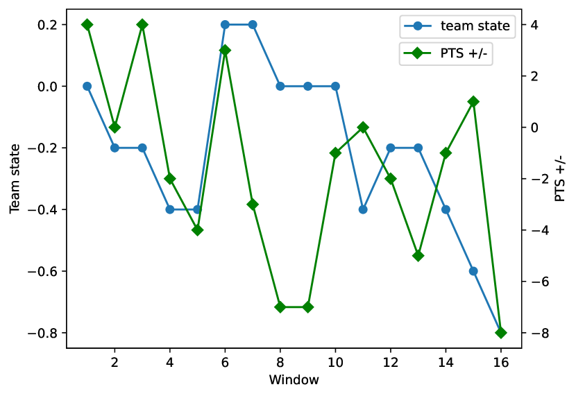
(d) Milwaukee Bucks vs Boston Celtics (15 May 2022)

Figure 17. Team collapse games

References

- (1)
- Baumeister and Showers (1986) Roy F Baumeister and Carolin J Showers. 1986. A review of paradoxical performance effects: Choking under pressure in sports and mental tests. European Journal of Social Psychology 16, 4 (1986), 361–383.
- Birnbaum (2008) Phil Birnbaum. 2008. Clutch hitting and the cramer test. The Baseball Research Journal 37 (2008), 71–76.
- Bishop (2006) Christopher M. Bishop. 2006. Pattern recognition and machine learning. Springer.
- Bradley and Terry (1952) Ralph Allan Bradley and Milton E Terry. 1952. Rank analysis of incomplete block designs: I. The method of paired comparisons. Biometrika 39, 3/4 (1952), 324–345.
- Bransen et al. (2019) Lotte Bransen, Pieter Robberechts, Jan Van Haaren, and Jesse Davis. 2019. Choke or shine? Quantifying soccer players’ abilities to perform under mental pressure. In Proceedings of the 13th MIT sloan sports analytics conference. 1–25.
- Cervone et al. (2016) Daniel Cervone, Alex D’Amour, Luke Bornn, and Kirk Goldsberry. 2016. A multiresolution stochastic process model for predicting basketball possession outcomes. J. Amer. Statist. Assoc. 111, 514 (2016), 585–599.
- Chen and Joachims (2016a) Shuo Chen and Thorsten Joachims. 2016a. Modeling intransitivity in matchup and comparison data. In Proceedings of the ninth acm international conference on web search and data mining. 227–236.
- Chen and Joachims (2016b) Shuo Chen and Thorsten Joachims. 2016b. Predicting matchups and preferences in context. In Proceedings of the 22nd ACM SIGKDD International Conference on Knowledge Discovery and Data Mining. 775–784.
- Chen et al. (2021) Wen-Cheng Chen, Wan-Lun Tsai, Huan-Hua Chang, Min-Chun Hu, and Wei-Ta Chu. 2021. Instant basketball defensive trajectory generation. ACM Transactions on Intelligent Systems and Technology (TIST) 13, 1 (2021), 1–20.
- D’Amour et al. (2015) Alexander D’Amour, Daniel Cervone, Luke Bornn, and Kirk Goldsberry. 2015. Move or Die: How Ball Movement Creates Open Shots in the NBA.
- Decroos et al. (2019) Tom Decroos, Lotte Bransen, Jan Van Haaren, and Jesse Davis. 2019. Actions speak louder than goals: Valuing player actions in soccer. In Proceedings of the 25th ACM SIGKDD international conference on knowledge discovery & data mining. 1851–1861.
- Dohmen (2008) Thomas J Dohmen. 2008. Do professionals choke under pressure? Journal of economic behavior & organization 65, 3-4 (2008), 636–653.
- Dong et al. (2012) Wen Dong, Alex Pentland, and Katherine A. Heller. 2012. Graph-Coupled HMMs for Modeling the Spread of Infection. In Proceedings of the Twenty-Eighth Conference on Uncertainty in Artificial Intelligence, Catalina Island, CA, USA, August 14-18, 2012, Nando de Freitas and Kevin P. Murphy (Eds.). AUAI Press, 227–236.
- Hill et al. (2010) Denise M Hill, Sheldon Hanton, Nic Matthews, and Scott Fleming. 2010. Choking in sport: A review. International Review of Sport and Exercise Psychology 3, 1 (2010), 24–39.
- Koller and Friedman (2009) Daphne Koller and Nir Friedman. 2009. Probabilistic graphical models: principles and techniques. MIT press.
- Langville and Meyer (2012) Amy N Langville and Carl D Meyer. 2012. Who’s# 1? The science of rating and ranking. Princeton University Press.
- Lucey et al. (2016) Patrick Lucey, Alina Bialkowski, Mathew Monfort, Peter Carr, and Iain Matthews. 2016. quality vs quantity: Improved shot prediction in soccer using strategic features from spatiotemporal data. In 8th MIT Sloan Sports Analytics Conference.
- Macdonald (2011) Brian Macdonald. 2011. A regression-based adjusted plus-minus statistic for NHL players. Journal of Quantitative Analysis in Sports 7, 3 (2011).
- Miller et al. (2014) Andrew Miller, Luke Bornn, Ryan Adams, and Kirk Goldsberry. 2014. Factorized Point Process Intensities: A Spatial Analysis of Professional. In ICML.
- Nguyen et al. (2023) Quang Nguyen, Ronald Yurko, and Gregory J Matthews. 2023. Here Comes the STRAIN: Analyzing Defensive Pass Rush in American Football with Player Tracking Data. arXiv preprint arXiv:2305.10262 (2023).
- Pan et al. (2012) Wei Pan, Wen Dong, Manuel Cebrian, Taemie Kim, James H Fowler, and Alex Sandy Pentland. 2012. Modeling dynamical influence in human interaction: Using data to make better inferences about influence within social systems. IEEE Signal Processing Magazine 29, 2 (2012), 77–86.
- Park and Newman (2005) Juyong Park and Mark EJ Newman. 2005. A network-based ranking system for US college football. Journal of Statistical Mechanics: Theory and Experiment 2005, 10 (2005), P10014.
- Parkin and Walsh (2017) Beth L Parkin and Vincent Walsh. 2017. Gunslingers, poker players, and chickens 2: Decision-making under physical performance pressure in subelite athletes. Progress in Brain Research 234 (2017), 317–338.
- Pelechrinis (2018) Konstantinos Pelechrinis. 2018. Linnet: Probabilistic lineup evaluation through network embedding. In Joint European Conference on Machine Learning and Knowledge Discovery in Databases. Springer, 20–36.
- Pelechrinis et al. (2016) Konstantinos Pelechrinis, Evangelos Papalexakis, and Christos Faloutsos. 2016. Sportsnetrank: Network-based sports team ranking. ACM KDD Workshop on Large-Scale Sports Analytics (2016).
- Pineda-Hernández (2022) Sònia Pineda-Hernández. 2022. How to play under pressure: EEG monitoring of mental activation training in a professional tennis player. Physiology & Behavior 250 (2022), 113784.
- Sabin (2021) R Paul Sabin. 2021. Estimating player value in American football using plus–minus models. Journal of Quantitative Analysis in Sports 17, 4 (2021), 313–364.
- Seidl et al. (2018) Thomas Seidl, Aditya Cherukumudi, Andrew Hartnett, Peter Carr, and Patrick Lucey. 2018. Bhostgusters: Realtime interactive play sketching with synthesized NBA defenses. In Proceeding of the 12th MIT Sloan Sports Analytics Conference, Boston, MA. Boston: MIT.
- Sicilia et al. (2019) Anthony Sicilia, Konstantinos Pelechrinis, and Kirk Goldsberry. 2019. Deephoops: Evaluating micro-actions in basketball using deep feature representations of spatio-temporal data. In Proceedings of the 25th ACM SIGKDD International Conference on Knowledge Discovery & Data Mining. 2096–2104.
- Solomonov et al. (2015) Yosef Solomonov, Simcha Avugos, and Michael Bar-Eli. 2015. Do clutch players win the game? Testing the validity of the clutch player’s reputation in basketball. Psychology of Sport and Exercise 16 (2015), 130–138.
- Thomas et al. (2013) AC Thomas, Samuel L Ventura, Shane T Jensen, and Stephen Ma. 2013. Competing process hazard function models for player ratings in ice hockey. The Annals of Applied Statistics (2013), 1497–1524.
- W Bassett (2007) Gilbert W Bassett. 2007. Quantile regression for rating teams. Statistical Modelling 7, 4 (2007), 301–313.
- Wallace et al. (2013) Scott Wallace, Steven B Caudill, and Franklin G Mixon Jr. 2013. Homo certus in professional basketball? Empirical evidence from the 2011 NBA Playoffs. Applied Economics Letters 20, 7 (2013), 642–648.
- Winston et al. (2022) Wayne L Winston, Scott Nestler, and Konstantinos Pelechrinis. 2022. Mathletics: How gamblers, managers, and fans use mathematics in sports. Princeton University Press.
- Yue et al. (2014) Yisong Yue, Patrick Lucey, Peter Carr, Alina Bialkowski, and Ian Matthews. 2014. Learning fine-grained spatial models for dynamic sports play prediction. In ICDM.
- Yurko et al. (2020) Ronald Yurko, Francesca Matano, Lee F Richardson, Nicholas Granered, Taylor Pospisil, Konstantinos Pelechrinis, and Samuel L Ventura. 2020. Going deep: models for continuous-time within-play valuation of game outcomes in American football with tracking data. Journal of Quantitative Analysis in Sports 16, 2 (2020), 163–182.