Signed Diverse Multiplex Networks: Clustering and Inference

Abstract

The paper introduces a Signed Generalized Random Dot Product Graph (SGRDPG) model, which is a variant of the Generalized Random Dot Product Graph (GRDPG), where, in addition, edges can be positive or negative. The setting is extended to a multiplex version, where all layers have the same collection of nodes and follow the SGRDPG. The only common feature of the layers of the network is that they can be partitioned into groups with common subspace structures, while otherwise all matrices of connection probabilities can be all different. The setting above is extremely flexible and includes a variety of existing multiplex network models as its particular cases. The paper fulfills two objectives. First, it shows that keeping signs of the edges in the process of network construction leads to a better precision of estimation and clustering and, hence, is beneficial for tackling real world problems such as analysis of brain networks. Second, by employing novel algorithms, our paper ensures equivalent or superior accuracy than has been achieved in simpler multiplex network models. In addition to theoretical guarantees, both of those features are demonstrated using numerical simulations and a real data example.

1 1. Introduction

1.1 1.1 Signed Generalized Random Dot Product Graph (SGRDPG) model

Stochastic network models appear in a variety of applications, including genetics, proteomics, medical imaging, international relationships, brain science and many more. In the last few decades, researchers developed a variety of ways to model those networks, imposing some restriction on the matrix of probabilities that generates random edges. The block models and the latent position graph settings are perhaps the most popular ways of modeling random graphs. In particular, the Generalized Random Dot Product Graph (GRDPG) model is a latent position graph model which has great flexibility. However, the GRDPG requires assumptions that are difficult to satisfy. In order to remove this shortcoming, below we introduce the Signed Generalized Random Dot Product Graph (SGRDPG) model and extend it to a multilayer setting.

Consider a undirected network with $n$ nodes and without self-loops. The GRDPG model refers to a network where the matrix of connection probabilities is of the form

$$P=UQU^{T},\quad Q=Q^{T}\in{\mathbb{R}}^{K\times K}.$$ (1)

Here $U\in{\mathbb{R}}^{n\times K}$ is a matrix with orthonormal columns, and $U$ and $Q$ are such that all entries of $P$ are in $[0,1]$. The GRDPG network model is very flexible and is known to have a variety of the network models as its particular cases: the Stochastic Block Model (SBM), the Degree Corrected Block Model (Gao et al. (2018)), the Popularity Adjusted Block Model (Koo et al. (2022), Noroozi et al. (2021)), the Mixed Membership Model (Airoldi et al. (2008), Cheng et al. (2017)), or the Degree Corrected Mixed Membership Model (Ke and Wang (2022)). If all eigenvalues of matrix $Q$ are positive, then model (1) reduces to the Random Dot Product Graph (RDPG) model (see, e.g., the survey in Athreya et al. (2018)). The RDPG and the GRDPG models (Athreya et al. (2018), Rubin-Delanchy et al. (2022)) have recently gained an increasing popularity.

Nevertheless, the condition that elements of matrix $P$ in (1) are indeed probabilities is not easy to satisfy. Indeed, unless a network is generated using one of the above mentioned block model scenarios and matrices $U$ and $Q$ are found later by using the Singular Value Decomposition (SVD), it is very difficult to guarantee that the elements of matrix $P$ are nonnegative. The latter is due to the fact that, in general, elements of matrix $U$ can be positive or negative. For this reason, here we propose the Signed Generalized Dot Product Graph (SGRDPG) model which generates an edge between nodes $i$ and $j$ with probability $|P_{i,j}|$ and the corresponding element of the adjacency matrix $A(i,j)$ can be zero, 1 or -1:

$${\mathbb{P}}(|A(i,j)|=1)=|P(i,j)|,\ \mbox{sign}(A(i,j))=\mbox{sign}(P(i,j)),$$

$$A(i,j)=A(i,j)\quad 1\leq i<j\leq n$$ (2)

It is easy to ensure that $|P(i,j)|\leq 1$ since the latter is guaranteed by the row norms of matrix $U$ being bounded by one and the eigenvalues of matrix $Q$ being in the interval $[-1,1]$. The setting above can be viewed as a particular case of a Weighted Graph introduced in Gallagher et al. (2023+). However, the Signed RGDPG model does not require special tools for its analysis, unlike the Weighted Graph model in Gallagher et al. (2023+), and can be easily extended to a multilayer context.

The purpose of the introduction of the Signed RGDPG model and its multilayer version is not limited to the fact that that non-negativity constraints are hard to satisfy. The signed networks has long been studied in the social sciences where relation between two nodes can be positive (”friendship”), or negative (”animosity”), or zero (”no relationship”). However, outside this field of study, the edges of the network are modeled as existing or non-existing leading to a “0-1” binary network.

One of the reasons of abandoning the signs while modeling a network is a prevailing balance theory which puts restrictions on the signs of the edges. In particular, the maxims ”an enemy of my enemy is my friend” and ”two of my friends cannot be enemies” lead to the fact that any closed triangle in a signed network can have either two or zero negative edges (strong balance). The allure of the strong balance formulation lies in the fact that strongly balanced networks are clusterable (Harary (1953)), i.e., the nodes can be divided into some number of disjoint sets such that all edges within sets are positive and all edges between sets are negative. This is, however, a sufficient condition while the necessary condition for clusterability is the so called weak balance (Davis (1967)), which requires that there are no closed loops in the network with exactly one negative edge.

A number of authors studied signed networks in a view of the balance theory and tested balance in real world networks and drew surprisingly different conclusions (see, e.g., Babul and Lambiotte (2023), Estrada and Benzi (2014), Feng et al. (2022), Gallo et al. (2023), Singh and Adhikari (2017), Kirkley et al. (2019) among others). For example, Kirkley et al. (2019), compared signed networks with ”null networks” that have the same edge locations and the same number of negative and positive edges, while the signs of the edges are assigned at random, and discovered that the networks in their examples are both strongly and weakly balanced. On the other hand, Feng et al. (2022) argued that many of the existing real world networks are not balanced. This particularly applies to biological networks, which are often constructed on the basis of correlation (or precision) matrices, elements of which can be positive or negative. There is no intrinsic reason for the balance in those networks, since it is possible that there are multiple tuples of nodes such that one or all three pairs in the tuple have negative correlations.

Therefore, in this paper we do not associate the signs distribution with any intrinsic pattern, as it is done in , e.g., Cucuringu et al. (2019), and, instead, just preserve the sign of each edge. Furthermore, we demonstrate below that keeping the signs in the process of construction of an, otherwise, binary network improves the accuracy of the statistical inference. On the other hand, we would like to point out that all intrinsic difficulties, associated with using Bernoulli rather than, say, Gaussian variables, remain in this case.

1.2 1.2  SGRDPG-equipped Diverse MultiPLEx network (DIMPLE-SRGDPG)

While in the early years of the field of stochastic networks, research mainly focused on studying a single network, in recent years the frontier moved to investigation of collection of networks, the so called multilayer network, which allows to study relationships between nodes with respect to various modalities (e.g., relationships between species based on food or space), or consists of network data collected from different individuals (e.g., brain networks). Although there are many different ways of modeling a multilayer network (see, e.g., an excellent review article of Kivela et al. (2014)), in this paper, we consider a Multiplex Network Model where all layers have the same set of nodes, and all the edges between nodes are drawn within layers, i.e., there are no edges connecting the nodes in different layers. Multiplex network models have a variety of applications such as brain networks (Sporns (2018)) where nodes are brain regions and layers are individuals, or trade networks (De Domenico et al. (2015)) where nodes and layers represent, respectively, various countries and commodities in which they are trading.

Many authors researched multiplex network models, imposing an array of restrictions of varying degree of severity. The simplest of the multiplex network models, the “checker board model” of Chi et al. (2020), assumes that all layers are equipped with the Stochastic Block Models, all layers have the same communities and there are only few distinct block connectivity matrices. On the other hand, the DIverse MultiPLEx Generalized Random Dot Product Graph (DIMPLE-GRDPG) in Pensky and Wang (2021) considers layers that follow the GRDPG model (Rubin-Delanchy et al. (2022)) and allows utmost variability in layers’ structures and connectivity patterns throughout the network.

The present paper follows this most general multiplex network model of Pensky and Wang (2021), and, in addition, allows edges to be equipped with signs. The objective of the paper is twofold: first, it shows that keeping signs of the edges in the process of network construction leads to a more accurate estimation and clustering; second, it demonstrates that, even for this extremely complex multilayer network, one can achieve similar or better inference precision, than has been obtained obtained for simpler multiplex network models.

Specifically, this paper studies a multiplex network where each layer follows the SGRDPG model introduced in (2). Consider an $L$-layer network on the same set of $n$ vertices $[n]\equiv\{1,\cdots,n\}$. The tensor of connection probabilities $\mathbf{P}\in[0,1]^{n\times n\times L}$ is formed by layers $P^{(l)}$, $l\in[L]$, which can be partitioned into $M$ groups, so that there exists a label function $s:[L]\to[M]$. It is assumed that the probability matrices $P^{(l)}$ of the layers of the network follow the SGRDPG model defined in (1) and (2), and that each group of layers is embedded in its own ambient subspace, but otherwise all matrices of connection probabilities can be different. Specifically, $P^{(l)}$, $l\in[L]$, are given by

$$P^{(l)}=U^{(m)}Q^{(l)}(U^{(m)})^{T},\quad m=s(l),$$ (3)

where $Q^{(l)}=(Q^{(l)})^{T}$, and $U^{(m)}$, $m\in[M]$, are matrices with orthonormal columns. Here, however, matrices $U^{(m)}$ and $Q^{(l)}$ are not required to ensure that elements of matrices $P^{(l)}$ are probabilities, but just that they lie in the interval $[-1,1]$, which is a much easier condition to satisfy. We shall call this setting the DIverse MultiPLEx Signed Generalized Random Dot Product Graph (DIMPLE-SGRDPG).

Here, one observes the adjacency tensor $\mathbf{A}\in\{0,1\}^{n\times n\times L}$ with layers $A^{(l)}$ such that $A{{}^{(l)}}(i,j)$ are independent from each other for $1\leq i<j\leq n$ and $l\in[L]$, $A{{}^{(l)}}(i,j)=A^{(l)}(j,i)$. and follow (2), i.e.,

$${\mathbb{P}}(|A^{(l)}(i,j)|=1)=|P^{(l)}(i,j)|,$$ (4)

$$\mbox{sign}(A^{(l)}(i,j))=\mbox{sign}(P^{(l)}(i,j))$$

The objective is to recover the between-layer clustering function $s:[L]\to[M]$ with the corresponding clustering matrix $S$, and the bases $U^{(m)}$ of the ambient subspaces in (3). Note that, however, the main task in the DIMPLE-SGRDPG model is the between-layer clustering. Indeed, if the groups of layers are correctly identified, then the layers with common subspace structures can be pooled together in a variety of ways, as it is done in Arroyo et al. (2021) or Pensky and Wang (2021). On the other hand, we do not estimate the matrices $Q^{(l)}$ in (3) since they act as nuisance parameters, as far as the inference on the structure of the network is concerned. If desired, those matrices can be recovered by standard methods (see, e.g., Athreya et al. (2018)).

1.3 1.3 Existing results and technical challenges

It turns out that the DIMPLE-SGRDPG model generalizes a multitude of multiplex network models developed in the last few years. As it was already noted above, if the matrices $P^{(l)}$ have all elements in the interval $[0,1]$ the model reduces to the DIMPLE-GRDPG setting, introduced and studied in Pensky and Wang (2021). Since the present paper is the first one to introduce the Signed GRDPG model, all subsequent papers in the discussion below offer some particular cases of the DIMPLE-GRDPG model in Pensky and Wang (2021).

In particular, if all layers share the same ambient subspace structure, i.e., $M=1$ in (3), the DIMPLE-GRDPG reduces to the COSIE model in Arroyo et al. (2021) and Zheng and Tang (2022). The multilayer random dot product graph featured in Jones and Rubin-Delanchy (2020), while not being an exact particular case of the DIMPLE-GRDPG, due to the probability matrices $P^{(l)}$ in the layers being asymmetric, can be reduced to COSIE by replacing $P^{(l)}$ by $P^{(l)}(P^{(l)})^{T}$. Furthermore, there is a multitude of papers that study SBM-equipped multiplex networks, which constitute particular cases of the DIMPLE-GRDPG (see an extensive discussion in Noroozi and Pensky (2022) and references therein). Furthermore, the multiplex network equipped with the Degree-Corrected Stochastic Blockmodels, featured in Agterberg et al. (2022), also reduces to the COSIE model with $M=1$, due to the fact that the positions of the diagonal weight matrices and the membership matrices can be interchanged in the presentation of the layer probability matrices.

The DIMPLE-GRDPG can also be viewed as a generalization of a time-varying network with the GRDPG-equipped layers (e.g., Athreya et al. (2022)). However, the inference in a multiplex network is much more difficult than in the respective dynamic network since, in a dynamic network, the layers are ordered according to time instances, while in a multiplex network the enumeration of layers is completely arbitrary. The latter makes techniques designed for dynamic networks unsuitable for the inference in the DIMPLE-GRDPG setting.

Furthermore, we should comment on the relationship of the DIMPLE-SGRDPG model to the low-rank tensor models. In those models, one can represent a low rank tensor using the Tucker decomposition with a low-dimensional core tensor and subsequently recover the subspaces and the core tensor using the Higher Order Orthogonal Iterations (HOOI) (see, e.g., Agterberg and Zhang (2022)), Han et al. (2022), Luo et al. (2021), Zhang and Xia (2018)). The papers cited above, however, assume the noise components to be Gaussian (or sub-Gaussian with particular parameters) which makes their results not transferable to sparse binary networks. Recently, Fan et al. (2022) and Jing et al. (2021) considered the Mixed MultiLayer Stochastic Block Model (MMLSBM), where the layers can be partitioned into $M$ groups, with each group of layers equipped with its unique SBM. The MMLSBM is a particular case of the DIMPLE-GRDPG in (3), where $Q^{(l)}\equiv Q^{(m)}$ depend on $m=s(l)$ only.

Note that in all the papers cited above, the probability tensor $\mathbf{P}$ is of low rank, with the subspace structures associated with the problems of interest, and the inference relies on application of HOOI (except in Fan et al. (2022) which uses an Alternating Minimization Algorithm). Nonetheless, our framework is not generated by a low rank tensor. Instead, (3) and (4) can be viewed as a signed binary tensor which, in expectation, due to matrices $Q^{(l)}$ being arbitrary, reduces to a partial multilinear structure as in, e.g., Section 5 of Luo et al. (2021). In this case, one can recover the subspaces associated with the low-rank modes with much better precision than the high-rank mode which, in our case, is associated with the network layer clustering.

Our paper can also be viewed as related to the papers that study shared structures in the layers, specifically, the common and the uncommon parts of the bases for the ambient subspaces, associated with groups of layers. However, the publications known to us, such as Levin et al. (2022) and MacDonald et al. (2021), consider a very different setting where the probabilities of connections are the same in all layers while noise distribution varies from one layer to another.

1.4 1.4  Our contributions

Our paper makes several key contributions.

1. To the best of our knowledge, our paper is the first one to introduce the very flexible signed SGRDPG network model and to extend it to the multilayer case. We are considering the most general case of the multiplex networks with latent position/block model equipped layers.

2. Our paper offers a novel strongly consistent between-layer clustering algorithm that works for the GRDPG and SGRDPG equipped multiplex networks. It develops a general theory under very simple and intuitive assumptions, and shows that the new methodology delivers equivalent or superior accuracy than has been achieved in simpler multiplex network models.

3. Simulations in the paper establish that the between-layer and the within-layer clustering algorithms deliver high precision in a finite parameter settings. In addition, our subspace recovery error compares favorably to the ones, derived for the simpler COSIE model in Arroyo et al. (2021) and Zheng and Tang (2022), due to employment of a different algorithm.

4. Our simulations and real data example confirm that, in the case when edges of the network can naturally be positive or negative, keeping signs of the edges in the process of network construction leads to better accuracy of estimation and clustering. Hence, is beneficial for tackling real world problems such as analysis of brain networks.

5. Since our setting includes majority of the popular network models as its particular cases, our approach removes the need for testing, which of the particular network models should be used for the layers. After the groups of layers with similar ambient subspace structures are identified, one can recover those common structures and subsequently estimate community assignments, if one suspects that a block model generated networks in the layers.

1.5 1.5 Notations and organization of the paper

We denote $a_{n}=O(b_{n})$ if $a_{n}\leq Cb_{n}$, $a_{n}=\omega(b_{n})$ if $a_{n}\geq cb_{n}$, $a_{n}\propto b_{n}$ if $cb_{n}\leq a_{n}\leq Cb_{n}$, where $0<c\leq C<\infty$ are absolute constants independent of $n$. Also, $a_{n}=o(b_{n})$ and $a_{n}=\Omega(b_{n})$ if, respectively, $a_{n}/b_{n}\to 0$ and $a_{n}/b_{n}\to\infty$ as $n\to\infty$. We use $C$ as a generic absolute constant independent of $n$, $L$, $M$ and $K$.

For any vector $v\in{\mathbb{R}}^{p}$, denote its $\ell_{2}$, $\ell_{1}$, $\ell_{0}$ and $\ell_{\infty}$ norms by $\|v\|$, $\|v\|_{1}$, $\|v\|_{0}$ and $\|v\|_{\infty}$, respectively. Denote by $1_{m}$ the $m$-dimensional column vector with all components equal to one.

For any matrix $A$, denote its spectral, Frobenius and $(2,\infty)$ norms by, respectively, $\|A\|$, $\|A\|_{F}$ and $\|A\|_{2,\infty}=\max\|A(i,:)\|$. Denote the eigenvalues and singular values of $A$ by $\lambda(A)$ and $\sigma(A)$, respectively. Let $\mbox{SVD}_{r}(A)$ be $r$ left leading eigenvectors of $A$. The column $j$ and the row $i$ of a matrix $A$ are denoted by $A(:,j)$ and $A(i,:)$, respectively. Let $\mbox{vec}(A)$ be the vector obtained from matrix $A$ by sequentially stacking its columns. Denote by $A\otimes B$ the Kronecker product of matrices $A$ and $B$. Denote the diagonal of a matrix $A$ by ${\rm diag}(A)$. Also, denote the $K$-dimensional diagonal matrix with $a_{1},\ldots,a_{K}$ on the diagonal by ${\rm diag}(a_{1},\ldots,a_{K})$. Denote ${\mathcal{O}}_{n,K}=\left\{A\in{\mathbb{R}}^{n\times K}:A^{T}A=I_{K}\right\}$, ${\mathcal{O}}_{n}={\mathcal{O}}_{n,n}$. Denote by ${\mathcal{C}}_{n,K}$ the set of clustering matrices $X\in\{0,1\}^{n\times K}$ that partition $n$ objects into $K$ clusters, where $X$ is a clustering matrix if it is binary and has exactly one 1 per row. Also, we denote an absolute constants independent of $n,K,L$ and $M$, which can take different values at different instances, by $C$.

For any tensor $\mathbf{X}\in{\mathbb{R}}^{n_{1}\times n_{2}\times n_{3}}$ and a matrix $A\in{\mathbb{R}}^{m\times n_{1}}$, their mode-1 product $\mathbf{X}\times_{1}\mathbf{A}$ is a tensor in ${\mathbb{R}}^{m\times n_{2}\times n_{3}}$ defined by

$$[\mathbf{X}\times_{1}A](j,i_{2},i_{3})=\sum_{i_{1}=1}^{n_{1}}\mathbf{X}(i_{1},i_{2},i_{3})A(j,i_{1}),\quad j\in[M].$$

The scalar product of tensors $\mathbf{X},\mathbf{Y}\in{\mathbb{R}}^{n_{1}\times n_{2}\times n_{3}}$ is

$$\langle\mathbf{X},\mathbf{Y}\rangle=\sum_{i_{1}=1}^{n_{1}}\sum_{i_{2}=1}^{n_{2}}\sum_{i_{3}=1}^{n_{3}}\mathbf{X}(i_{1},i_{2},i_{3})\mathbf{Y}(i_{1},i_{2},i_{3})$$

The rest of the paper is organized as follows. Section 2 introduces a natural generative mechanism for a network that follows the DIMPLE-SGDPG model and presents algorithms for its analysis. Specifically, Section 2.3 suggests a novel between-layer clustering algorithm, while Section 2.4 examines techniques for fitting subspaces in groups of layers. Section 3 provides theoretical guarantees for the methodologies in Section 2, in particular, the upper bounds on the between-layer clustering errors (Section 3.2), the subspace fitting errors (Section 3.3), and the errors in the special case of the Stochastic Block Model and the Mixed Membership Model (Section 3.4). Section 4 considers finite sample studies of the proposed model and techniques designed for it, as well as its comparison to simpler but related previously investigated models. Section 5 illustrates the material in the paper with the real data example that demonstrates the advantage of keeping the edges’ signs in the process of network construction. Proofs for all statements of the paper can be found in Section 6.

2 2 Clustering and estimation techniques

2.1 2.1  The DIMPLE-SGRDPG network: generation and assumptions

Successful estimation and clustering in (3) is possible only if the subspace bases matrices $U^{(m)}$ in the groups of layers are not too similar. While one can postulate the necessary assumptions, as it is done in, e.g., Jing et al. (2021), and then make a reader wonder how easy it is to satisfy them, in what follows we propose a simple non-restrictive generative mechanism for forming a network that would guarantee successful inference. For obtaining SGRDPG networks in each of the layers, we follow the standard protocols of Arroyo et al. (2021).

For each layer $l\in[L]$, we generate its group membership as

$$s(l)\sim{\rm Multinomial}(\vec{\pi}),$$ (5)

$$\vec{\pi}=(\pi_{1},...,\pi_{M})\in[0,1]^{M},\ \pi_{1}+...+\pi_{M}=1.$$

In order to create the probability tensor $\mathbf{P}$, we generate $M$ matrices $X^{(m)}\in[-1,1]^{n\times K_{m}}$ with i.i.d. rows:

$$X^{(m)}(i,:)\sim\mbox{i.i.d.}\,f_{m},\ \ {\mathbb{E}}(X^{(m)}(i,:))=\mu^{(m)},$$ (6)

$$\mbox{Cov}(X^{(m)}(i,:))=\Sigma^{(m)},\ \ m\in[M],\ i\in[n]$$

where $f_{m}$ is a probability distribution on a subset of $[-1,1]^{K_{m}}$. Subsequently, we consider a collection of symmetric matrices $B^{(l)}\in{\mathbb{R}}^{K_{m}\times K_{m}}$, $m=s(l)$, $l\in[L]$, and form the layer probability matrices $P^{(l)}$ as

$$P^{(l)}=X^{(m)}B^{(l)}(X^{(m)})^{T}.$$ (7)

It is easy to see that (7) is equivalent to the model (3). Indeed, if $X^{(m)}=U_{X}^{(m)}D_{X}^{(m)}O_{X}^{(m)}$ is the SVD of $X^{(m)}$, then (7) can be rewritten as (3) with

$$Q^{(l)}=D_{X}^{(m)}O_{X}^{(m)}B^{(m)}(O_{X}^{(m)})^{T}D_{X}^{(m)},$$ (8)

$$U^{(m)}=U_{X}^{(m)},\ \ m=s(l),\ l\in[L].$$

Note that we do not assume the elements of matrices $P^{(l)}$ to be non-negative: we merely require that entries of $P^{(l)}$ lie between -1 and 1. It is relatively easy to satisfy this assumption. In particular, if $f_{m}$ is a distribution on the $K_{m}$-dimensional unit ball ${\mathcal{B}}(K_{m})$ and all singular values of $B^{(l)}$ lie in $[-1,1]$, then $P^{(l)}(i,j)\in[-1,1]$, $i,j\in[n]$. Observe also, that since $X^{(m)}$ and $B^{(l)}$ are defined up to a scaling constant, in what follows, we assume that $X^{(m)}(i,:)\in{\mathcal{B}}(K_{m})$, and model sparsity via matrices $B^{(l)}$, $l\in[L]$. We impose the following assumptions:

A1. Vector $\vec{\pi}=(\pi_{1},...,\pi_{M})$ is such that $\underline{c}_{\pi}\,M^{-1}\leq\pi_{m}\leq\bar{c}_{\pi}\,M^{-1}$, $m\in[M]$.

A2. Distributions $f_{m}$, $m\in[M]$, are supported on the $K_{m}$-dimensional unit balls ${\mathcal{B}}(K_{m})$. Here, $\displaystyle{K=\max_{m}K_{m}}$ and $\displaystyle{K\leq C_{K}\min_{m}K_{m}}$ for some constant $C_{K}$.

A3. Covariance matrices $\Sigma^{(m)}$ satisfy

$$0<\underline{c}\leq\lambda_{\min}(\Sigma^{(m)})\leq\lambda_{\max}(\Sigma^{(m)})\leq\bar{c}<\infty,\ \ m\in[M].$$ (9)

A4. The number of layers $L$ grows at most polynomially with respect to $n$, specifically, for some constant $\tau_{0}$

$$L\leq n^{\tau_{0}},\quad 0<\tau_{0}<\infty.$$ (10)

A5. For some positive constants $\underline{C}$ and $\bar{C}$, $0<\underline{C}\leq\bar{C}<\infty$ , one has

$$B^{(l)}=\rho_{n}B^{(l)}_{0}\quad\mbox{with}\quad\sigma_{\min}(B^{(l)}_{0})\geq\underline{C}_{B}>0.$$ (11)

Note that Assumption A1 as well as conditions on $K_{m}$ are always satisfied if $M$ is a constant independent of $L$ and $n$. The constants in Assumptions A3 and A5 can be modified to depend on $K_{m}$. However, this will make the notations too cumbersome. For this reason, we impose uniform bounds in Assumptions A3 and A5. Again, if $M$ and $K_{m}$ are constants independent of $L$ and $n$, those constraints are easily justifiable. Assumption A4 is hardly restrictive and is relatively common. Indeed, Jing et al. (2021) assume that $L\leq n$, so, in their paper, (10) holds with $\tau_{0}=1$. We allow any polynomial growth of $L$ with respect to $n$.

There are many ways of generating rows $X^{(m)}(i,:)\in{\mathcal{B}}(K_{m})$ of matrices $X^{(m)}$, $i\in[n]$, $m\in[M]$, satisfying conditions (6) and (9). Below are some examples, where we suppress the index $i$.

1. $f_{m}$ is a truncated normal distribution: $\xi\sim f_{m}$ is obtained as $\xi=\eta/\|\eta\|$ where $\eta\sim{\mathcal{N}}(0,\Sigma)$, the normal distribution with the mean 0 and covariance $\Sigma$.

2. Generate a vector $\eta\in[0,1]^{K+1}$ as $\eta\sim{\rm Multinomial}(\vec{\varpi})$, where $\vec{\varpi}=(\varpi_{1},...,\varpi_{K+1})$, $\varpi_{k}>0$, $\varpi_{1}+...+\varpi_{K+1}=1$. Set $\xi$ to be equal to the first $K$ components of $\eta$.

3. Generate a vector $\eta\in[0,1]^{K+1}$ as $\eta\sim{\rm Dirichlet}(\vec{\varpi})$, where $\vec{\varpi}=(\varpi_{1},...,\varpi_{K+1})$, $0\leq\varpi_{k}\leq 1$, $\varpi_{1}+...+\varpi_{K+1}=1$. Set $\xi$ to be equal to the first $K$ components of $\eta$

Note that Examples 2 and 3 bring to mind, respectively, the Stochastic Block Model (SBM) and the Mixed Membership Model (MMM), where the last column of the community assignment matrix $X^{(m)}$ is missing. Indeed, in the case of the SBM or the MMM, rows of matrix $X^{(m)}$ sum to one, which means that covariance matrix of the rows of $X^{(m)}$ is singular and does not satisfy Assumption A2. However, as we see later in Section 3.4, our methodology can handle the SBM or the MMM equipped networks, although Assumption A2 does not hold in those cases.

2.2 2.2 Disentangling the DIMPLE-SGRDPG network: the between-layer clustering

Although matrices $X^{(m)}$ and, hence, $U_{X}^{(m)}$ are different for different values of $m$, they are too similar for ensuring a reliable separation of layers of the network, due to the common mean $\mu^{(m)}$ of rows of $X^{(m)}$, which implies that ${\mathbb{E}}(X^{(m)})=1_{n}\mu^{(m)}$, $m\in[M]$. For this reason, we “de-bias” the layers by removing this common mean and replacing $X^{(m)}$ with $\widetilde{X}^{(m)}=X^{(m)}-1_{n}\bar{X}^{(m)}$, where $\bar{X}^{(m)}$ is the sample mean of the rows of $X^{(m)}$. By introducing a projection operator $\Pi=n^{-1}1_{n}1_{n}^{T}$, we can rewrite $\widetilde{X}^{(m)}$ as

$$\widetilde{X}^{(m)}=X^{(m)}-\Pi X^{(m)}=\Pi^{\bot}X^{(m)},\quad\Pi:=n^{-1}1_{n}1_{n}^{T}.$$ (12)

It is easy to see that for $m\in[M]$,  $l\in[L]$

$$\widetilde{P}^{(l)}=\Pi^{\bot}P^{(l)}\Pi^{\bot}=\widetilde{X}^{(m)}B^{(l)}(\widetilde{X}^{(m)})^{T},\ \ s(l)=m.$$ (13)

Consider the SVDs of $\widetilde{X}^{(m)}$ and $\widetilde{P}^{(l)}$:

$$\widetilde{X}^{(m)}=\widetilde{U}^{(m)}\widetilde{D}^{(m)}(\widetilde{O}^{(m)})^{T},\ \ \widetilde{P}^{(l)}=\widetilde{U}_{P}^{(l)}D_{P}^{(l)}(\widetilde{U}_{P}^{(l)})^{T},$$ (14)

where $\widetilde{O}^{(m)}\in{\mathcal{O}}_{K_{m}}$. Due to the relation $\widetilde{P}^{(l)}=\widetilde{U}^{(m)}\widetilde{B}^{(l)}\widetilde{U}^{(m)}$, where $\widetilde{B}^{(l)}=\widetilde{D}^{(m)}(\widetilde{O}^{(m)})^{T}B^{(l)}\widetilde{O}^{(m)}\widetilde{D}^{(m)}$, one can rewrite the SVD of $\widetilde{P}^{(l)}$ using the SVD of $\widetilde{B}^{(l)}$:

$$\widetilde{B}^{(l)}=\widetilde{U}_{B}^{(l)}\widetilde{D}_{B}^{(l)}(\widetilde{U}_{B}^{(l)})^{T},\ \widetilde{P}^{(l)}=\widetilde{U}^{(m)}\widetilde{U}_{B}^{(l)}\widetilde{D}_{B}^{(l)}(\widetilde{U}^{(m)}\widetilde{U}_{B}^{(l)})^{T}$$ (15)

with $\widetilde{U}_{B}^{(l)}\in{\mathcal{O}}_{K_{m}}$. Hence, it follows from (14) and (15) that $D_{P}^{(l)}=\widetilde{D}_{B}^{(l)}$ and

$$\widetilde{U}^{(m)}(\widetilde{U}^{(m)})^{T}=\widetilde{U}_{P}^{(l)}(\widetilde{U}_{P}^{(l)})^{T},\quad s(l)=m,$$ (16)

so that, the values of $\widetilde{U}_{P}^{(l)}(\widetilde{U}_{P}^{(l)})^{T}$ are unique for each group of layers $m\in[M]$.

It turns out that $\widetilde{U}^{(m)}(\widetilde{U}^{(m)})^{T}$ are dissimilar enough to allow one to separate the network layers into groups. For $l,l_{1},l_{2}\in[L]$, denote

$$\theta^{(l)}=\mbox{vec}(\widetilde{U}_{P}^{(l)}(\widetilde{U}_{P}^{(l)})^{T}),\quad\Theta(l_{1},l_{2})=\langle\theta^{(l_{1})},\theta^{(l_{2})}\rangle.$$ (17)

Then, the following statement is true.

Lemma 1.

Let Assumptions A1–A4 hold. If $n$ is large enough, then, for any fixed constant $\tau$, with probability at least $1-C_{0}M\,n^{-\tau}$, one has

$$\Theta(l_{1},l_{2})=K_{m}\quad s(l_{1})=s(l_{2})=m,$$ if (18)

$$\max_{l_{1},l_{2}}|\Theta(l_{1},l_{2})|\leq C_{1}\,K\,n^{-1}\,\log n s(l_{1})\neq s(l_{2}),$$ if (19)

where constants $C_{0}$ and $C_{1}$ depend only on $\tau$ and the constants in Assumptions A1–A4.

The formal proof of Lemma 1 is given in the Appendix. Below, we give a brief explanation why it is true. If $s(l_{1})=s(l_{2})=m$, then $\Theta(l_{1},l_{2})=\|\theta^{(m)}\|^{2}=\|\mbox{vec}(\widetilde{U}^{(m)}(\widetilde{U}^{(m)})^{T})\|^{2}$, and it is easy to show that the first relation in (18) holds. In order to justify (19), consider the sample covariance matrices $\widehat{\Sigma}^{(m)}$ with ${\mathbb{E}}(\widehat{\Sigma}^{(m)})=\Sigma^{(m)}$. If $n$ is large enough, matrices $\widehat{\Sigma}^{(m)}$ are both non-singular, and it follows from (14) that

$$\widehat{\Sigma}^{(m)}=\frac{(\widetilde{X}^{(m)})^{T}\widetilde{X}^{(m)}}{n-1}=\frac{\widetilde{O}^{(m)}\,(\widetilde{D}^{(m)})^{2}(\widetilde{O}^{(m)})^{T}}{n-1}.$$ (20)

Denoting $\left(\widehat{\Sigma}^{(m)}\right)^{1/2}=(n-1)^{-1/2}\,\widetilde{D}^{(m)}(\widetilde{O}^{(m)})^{T}$ and $\left(\widehat{\Sigma}^{(m)}\right)^{-1/2}=(n-1)^{1/2}\,\widetilde{O}^{(m)}(\widetilde{D}^{(m)})^{-1}$, derive that

$$\widetilde{U}^{(m)}=(n-1)^{-1/2}\,\widetilde{X}^{(m)}\,\left(\widehat{\Sigma}^{(m)}\right)^{-1/2}.$$ (21)

It turns out that matrices $\widetilde{X}^{(m)}$, $m\in[M]$, are dissimilar enough to allow separation of layers. In particular, the proof of (19) is based on the fact that, if $n$ is large enough, the singular values of the true and the sample covariance matrices are close to each other and that, with high probability
$\displaystyle\max_{l_{1}\neq l_{2}}\,|\Theta(l_{1},l_{2})|=O\left(n^{-2}\,\|(\widetilde{X}^{(m_{1})})^{T}\widetilde{X}^{(m_{2})}\|_{F}^{2}\right)=O\left(n^{-1}\,\log n\right).$ Note that, since the values of $\Theta(l_{1},l_{2})$ in (18) and (19) do not depend on matrices $B^{(l)}$, they are not affected by sparsity factor $\rho_{n}$, so their separation relies on the number $n$ of nodes being large enough. Nevertheless, the accuracy of their sample counterparts depends on the sparsity factor $\rho_{n}$.

2.3 2.3  The between-layer clustering algorithm

It is easy to see that Lemma 1 offers a path for the between-layer clustering. Consider proxies $\widetilde{A}^{(l)}=\Pi^{\bot}A^{(l)}\Pi^{\bot}$ for $\widetilde{P}^{(l)}$ in (13) and their full SVDs $\widetilde{A}^{(l)}=\widetilde{U}_{A}^{(l)}\widetilde{D}_{A}^{(l)}(\widetilde{U}_{A}^{(l)})^{T}$, $l\in[L]$. Note that $\mbox{rank}(P^{(l)})=K_{m}$ where $m=s(l)$, so columns of $\widetilde{U}_{A}^{(l)}$, beyond the first $K_{m}$ ones, estimate pure noise. Since we do not know the grouping of the layers in advance, we instead have to deal with $K^{(l)}=\mbox{rank}(P^{(l)})$ where, of course, $K^{(l)}=K_{m}$ if $s(l)=m$. Specifically, we form matrices

$$\widehat{U}_{A}^{(l)}=SVD_{K^{(l)}}(\widetilde{A}^{(l)}),\quad\widetilde{A}^{(l)}=\Pi^{\bot}A^{(l)}\Pi^{\bot},$$ (22)

and, subsequently, construct vectors $\hat{\theta}^{(l)}$ and a matrix $\widehat{\Theta}$ with components $\widehat{\Theta}(l_{1},l_{2})$, $l,l_{1},l_{2}\in[L]$

$$\hat{\theta}^{(l)}=\mbox{vec}\left(\widehat{U}_{A}^{(l)}(\widehat{U}_{A}^{(l)})^{T}\right),\quad\widehat{\Theta}(l_{1},l_{2})=\langle\hat{\theta}^{(l_{1})},\hat{\theta}^{(l_{2})}\rangle.$$ (23)

While straightforward clustering of matrix $\widehat{\Theta}$ does not guarantee strong consistency for grouping of the network layers, one can attain it by applying the Semidefinite Programming (SDP), as an intermediate step (Gartner and Matousek (2012)). Specifically, we solve the following SDP problem:

$$\widehat{Y}= \mbox{argmax}\langle Y,\widehat{\Theta}-T\,1_{L}1_{L}^{T}\rangle$$

$${\rm subject\ to}$$ (24)

$$Y\in[0,1]^{L\times L}\ \mbox{is positive semidefinite}$$

$$Y(i,i)=1,\quad i\in[L]$$

After that, we apply spectral clustering to the matrix $\widehat{Y}$, partitioning $L$ layers into $M$ groups. The procedure above is summarized by Algorithm 1.

Algorithm 1  The between-layer clustering

Input: Adjacency tensor $\mathbf{A}\in\{0,1\}^{n\times n\times L}$; number of groups of layers $M$; ambient dimension $K^{(l)}$ of each layer $l\in[L]$; threshold $T$; parameter $\epsilon$

Output: Estimated clustering function $\hat{s}:[L]\to[M]$ for groups of layers

Steps:
1: Find matrices $\widehat{U}_{A}^{(l)}=\mbox{SVD}_{K^{(l)}}(\widetilde{A}^{(l)})$ of $K^{(l)}$ left leading singular vectors of matrices $\widetilde{A}^{(l)}=\Pi^{\bot}A^{(l)}\Pi^{\bot}$, $l\in[L]$

2: Form vectors $\hat{\theta}^{(l)}=\mbox{vec}(\left(\widehat{U}_{A}^{(l)}(\widehat{U}_{A}^{(l)})^{T}\right)$, $l\in[L]$

3: Form matrix $\widehat{\Theta}$ with elements $\widehat{\Theta}(l_{1},l_{2})=\langle\hat{\theta}^{(l_{1})},\hat{\theta}^{(l_{2})}\rangle$, $l_{1},l_{2}\in[L]$

4: Solve the SDP problem (24) and obtain matrix $\widehat{Y}$

5: Obtain matrix $\widehat{V}=\mbox{SVD}_{M}(\widehat{Y})\in{\mathcal{O}}_{L,M}$ of $M$ leading singular vectors of matrix $\widehat{Y}$

6: Cluster $L$ rows of $\widehat{V}$ into $M$ clusters using $(1+\epsilon)$-approximate $K$-means clustering. Obtain estimated clustering function $\hat{s}$

Remark 1.

Unknown number of layers. While Algorithm 1 assumes $M$ to be known, in many practical situations this is not true, and the value of $M$ has to be discovered from data. Identifying the number of clusters is a common issue in data clustering, and it is a separate problem from the process of actually solving the clustering problem with a known number of clusters. There are many ways for estimating the number of clusters, for instance, by evaluation of the clustering error in terms of an objective function, as in, e.g., Zhang et al. (2012), or by monitoring the eigenvalues of the non-backtracking matrix or the Bethe Hessian matrix, as it is done in Le and Levina (2015).

Remark 2.

Unknown ambient dimensions.  In this paper, for the purpose of methodological developments, we assume that the ambient dimension $K^{(l)}$ (number of communities in the case of the DIMPLE model) of each layer of the network is known. This is a common assumption, and everything in the Remark 1 can also be applied to this case. Here, $K^{(l)}=K_{m}$ with $m=c(l)$. One can, of course, can assume that the values of $K_{m}$, $m\in[M]$, are known. However, since group labels are interchangeable, in the case of non-identical subspace dimensions (numbers of communities), it is hard to choose, which of the values corresponds to which of the groups. This is actually the reason why Jing et al. (2021) and Fan et al. (2022), who imposed this assumption, used it only in theory, while their simulations and real data examples are all restricted to the case of equal number of communities in all layers $K_{m}=K$, $m\in[M]$. On the contrary, knowledge of $K^{(l)}$ allows one to deal with different ambient dimensions (number of communities) in the groups of layers in simulations and real data examples. Specifically, one can infer the ambient dimension in each group of layers using the ScreeNOT technique of Donoho et al. (2023).

2.4 2.4 Fitting invariant subspaces in groups of layers

If we knew the true clustering matrix $S\in{\mathcal{C}}_{L,M}$ and the true probability tensor $\mathbf{P}\in{\mathbb{R}}^{n\times n\times L}$ with layers $P^{(l)}$ given by (3), then we could average layers with identical subspace structures. Precision of estimating matrices $U^{(m)}$, however, depends on whether the eigenvalues of $Q^{(l)}$ with $s(l)=m$ in (3) add up. Since the latter is not guaranteed, one can alternatively add the squares $G^{(l)}=(P^{(l)})^{2}$, obtaining for $m\in[M]$

$$\sum_{s(l)=m}G^{(l)}=\sum_{s(l)=m}(P^{(l)})^{2}=\sum_{s(l)=m}U^{(m)}\,(Q^{(l)})^{2}\,(U^{(m)})^{T}.$$

In this case, the eigenvalues of $(Q^{(l)})^{2}$ are all positive which ensures successful recovery of matrices $U^{(m)}$. Note that, however, $(A^{(l)})^{2}$ is not an unbiased estimator of $(P^{(l)})^{2}$. Indeed, while ${\mathbb{E}}[(A^{(l)})^{2}(i,j)]=[(P^{(l)})^{2}(i,j)]$ for $i\neq j$, for the diagonal elements, one has

$${\mathbb{E}}\left[(A^{(l)})^{2}(i,i)\right]=(P^{(l)})^{2}(i,i)+\sum_{j}\left[|P^{(l)}(i,j)|-(P^{(l)})^{2}(i,j)\right].$$

Therefore, we de-bias the squares $(A^{(l)})^{2}$ by subtracting the diagonal matrices $\widehat{D}^{(l)}$ with elements

$$\widehat{D}^{(l)}(i,i)=\sum_{j=1}^{n}|A^{(l)}(i,j)|,\quad\widehat{D}^{(l)}(i,j)=0\ \ \mbox{if}\ \ i\neq j.$$

Hence, in order to estimate matrices $U^{(m)}$, $m\in[M]$, we construct a tensor $\widehat{\mathbf{G}}\in{\mathbb{R}}^{n\times n\times L}$ with layers $\widehat{G}^{(l)}=\widehat{\mathbf{G}}(:,:,l)$ of the form

$$\widehat{G}^{(l)}=\left(A^{(l)}\right)^{2}-\widehat{D}^{(l)},\quad l\in[L].$$ (25)

Subsequently, we combine layers of the same types, obtaining tensor $\widehat{\mathbf{H}}\in{\mathbb{R}}^{n\times n\times M}$. In particular, let $\widehat{S}\in{\mathcal{C}}_{L,M}$ be the estimated clustering matrix corresponding to the estimated clustering function $\hat{s}$ in Algorithm 1. Construct tensor $\widehat{\mathbf{H}}\in{\mathbb{R}}^{n\times n\times M}$ with layers $\widehat{H}^{(m)}$, $m\in[M]$:

$$\widehat{\mathbf{H}}=\widehat{\mathbf{G}}\times_{3}\widehat{W}^{T},\quad\widehat{W}=\widehat{S}\,(\widehat{S}^{T}\,\widehat{S})^{-1/2}.$$ (26)

After that, estimate $U^{(m)}$ by the matrix of $K_{m}$ leading singular vectors of $\widehat{H}^{(m)}$:

$$\widehat{U}^{(m)}=\mbox{SVD}_{K_{m}}(\widehat{H}^{(m)}),\quad m\in[M].$$ (27)

The procedure is summarized in Algorithm 2.

Algorithm 2  Estimating invariant subspaces

Input: Adjacency tensor $\mathbf{A}\in\{0,1\}^{n\times n\times L}$; number of groups of layers $M$; ambient dimensions $K_{m}$ of a group of layers $m\in[M]$; estimated layer clustering matrix $\widehat{S}\in{\mathcal{C}}_{L,M}$

Output: Estimated invariant subspaces $\widehat{U}^{(m)}$, $m\in[M]$

Steps:
1: Construct tensor $\widehat{\mathbf{G}}$ with layers $\widehat{G}^{(l)}$, $l\in[L]$, given by (25)

2: Construct tensor $\widehat{\mathbf{H}}$ with layers $\widehat{H}^{(m)}$, $m\in[M]$, using formula (26)

3: For each $m\in[M]$, find $\widehat{U}^{(m)}$ using formula (27)

Remark 3.

Estimating ambient subspaces by spectral embedding.  Note that one can estimate bases $\widehat{U}^{(m)}$ of the ambient subspaces using spectral embedding, as it was done in, e.g., Arroyo et al. (2021) or Jones and Rubin-Delanchy (2020). Specifically, for this purpose one would place, side by side, the adjacency matrices $A^{(l)}$ with $\hat{s}(l)=m$, forming matrix $\widehat{H}_{A}^{(m)}\in\{0,1\}^{n\times n\widehat{L}_{m}}$, where $\widehat{L}_{m}$ is the estimated number of layers in a group $m\in[M]$. Afterwards, one estimates $U^{(m)}$ by $\widehat{U}^{(m)}=\mbox{SVD}_{K_{m}}(\widehat{H}_{A}^{(m)})$. While this methodology has theoretical properties similar to Algorithm 2, in our simulations, we discovered that Algorithm 2 delivers somewhat higher accuracy. We elaborate on this topic in Section 4.2 of the paper.

3 3  Theoretical analysis

3.1 3.1 Error measures

In this section, we study the between-layer clustering error rates of the Algorithm 1 and the error of estimation of invariant subspaces of Algorithm 2. Since clustering is unique only up to a permutation of cluster labels, denote the set of $K$-dimensional permutation functions of $[K]$ by $\aleph(K)$, and the set of $(K\times K)$ permutation matrices by $\mathfrak{F}(K)$. The misclassification error rate of the between-layer clustering is then given by

$$R_{BL}=(2\,L)^{-1}\ \min_{\mathscr{P}\in\mathfrak{F}(M)}\ \|\widehat{S}-S\,\mathscr{P}\|^{2}_{F}.$$ (28)

In order to assess the accuracy of estimating matrices $U^{(m)}$ by $\widehat{U}^{(m)}$, $m\in[M]$, we use the $\sin\Theta$ distances that allow to take into account that matrices $\widehat{U}^{(m)}$ are unique only up to an arbitrary rotation. The $\sin\Theta$ distances between two subspaces with orthonormal bases $U\in{\mathcal{O}}_{n,K}$ and $\widehat{U}\in{\mathcal{O}}_{n,K}$, respectively, are defined as follows (Wainwright (2019)). Suppose the singular values of $U^{T}\widehat{U}$ are $\sigma_{1}\geq\sigma_{2}\geq...\geq\sigma_{K}>0$. The quantitative measures of the distance between the column spaces of $U$ and $\widehat{U}$ are then

$$\|\sin\Theta(U,\widehat{U})\|=\left(1-\sigma_{K}^{2}(U^{T}\widehat{U})\right)^{1/2},$$ (29)

$$\|\sin\Theta(U,\widehat{U})\|_{F}=\left(K-\|U^{T}\widehat{U})\|^{2}_{F}\right)^{1/2}.$$

We also define

$$D(U,\widehat{U};2,\infty)=\min_{W\in{\mathcal{O}}_{K}}\|\widehat{U}\,W-U\|_{2,\infty}$$ (30)

and observe (see, e.g., Cai and Zhang (2018a)) that $D(U,\widehat{U};2,\infty)\leq\sqrt{2}\,\|\sin\Theta(U,\widehat{U})\|$ and also

$$\|\sin\Theta(U,\widehat{U})\|\leq\|\widehat{U}\widehat{U}^{T}-UU^{T}\|\leq\sqrt{2}\,\|\sin\Theta(U,\widehat{U})\|.$$

Since the numbering of groups of layers is defined up to a permutation, we need to minimize those errors over the permutation of labels. In particular, we measure the precision of subspace estimation by

$$R_{U,2,\infty}=\min_{\aleph(M)}\ \max_{m\in[M]}\,D\left(U^{(m)},\widehat{U}^{(\aleph(m))};2,\infty\right)$$ (31)

$$R_{U,ave}=\frac{1}{M}\ \min_{\aleph(M)}\ \sum_{m=1}^{M}\,\|\sin\Theta\left(U^{(m)},\widehat{U}^{(\aleph(m))}\right)\|_{F}^{2}$$ (32)

Note that one can also measure the accuracy of subspace estimation by the maximum discrepancy over groups of layers in operational norm

$$R_{U,max}=\min_{\aleph(M)}\ \max_{m\in[M]}\,\left\|\sin\Theta\left(U^{(m)},\widehat{U}^{(\aleph(m))}\right)\right\|$$ (33)

However, since $0.5\,R^{2}_{U,2,\infty}\leq R^{2}_{U,max}\leq R^{2}_{U,ave}$, one can easily obtain the lower and the upper bounds for $R_{U,max}$, using (31) and (32).

3.2 3.2  The accuracy of the between-layer clustering

Successful between-layer clustering relies on the fact that the elements of the true Gramm matrix $\Theta(l_{1},l_{2})$ in (18) and (19) are large when $s(l_{1})=s(l_{2})$ and small otherwise. In practice, those values are unavailable, and one has to use their sample substitutes in Algorithm 1. It is obvious that the between-layer clustering errors depend on whether matrix $\widehat{\Theta}$ in (23) inherits the properties of $\Theta$. It turns out that the latter is true if $n$ is large enough and the layers are not too sparse. Specifically, the following statement holds.

Lemma 2.

If the layers of the network are moderately sparse, so that

$$n\,\rho_{n}\geq C_{\rho}\,\log n,$$ (34)

then, if $n$ is large enough, for any fixed constant $\tau$, uniformly, with probability at least $1-C_{\tau}\,n^{-(\tau-\tau_{0})}$, one has

$$\widehat{\Theta}(l_{1},l_{2})\geq K_{m}\left[1-\frac{C_{2}}{\sqrt{n\,\rho_{n}}}\right]\ \mbox{if}\ s(l_{1})=s(l_{2})=m,$$ (35)

$$|\widehat{\Theta}(l_{1},l_{2})|\leq C_{3}K\,(n\,\rho_{n})^{-1/2} \mbox{if}\ s(l_{1})\neq s(l_{2})$$ (36)

where constants $C_{\tau}$, $C_{2}$ and $C_{3}$ depend only on $\tau$ and the constants in Assumptions A1–A5.

While we state that $n$ has to be large enough in order Lemma 2 holds, we provide an exact inequality for the lower bound on $n$ in formula (67) of Section 6.3, which ensures that Lemma 2 and subsequent statements are valid.

Note that condition (34) is very common in the random networks models. If a random network follows the SBM, then condition (34) is necessary and sufficient for adequate community recovery (Gao et al. (2017)). Since in our multiplex network the layers are grouped on the basis of subspace similarities, it is only natural that assumption (34) appears in our theory. Indeed, this assumption is present in a number of papers that consider simpler multilayer GRDPG models, such as COSIE in Arroyo et al. (2021) and Zheng and Tang (2022), or the Multilayer Degree-Corrected Stochastic Blockmodels in Agterberg et al. (2022).

Theorem 1.

Let layer assignment function $\hat{s}$ be obtained by Algorithm 1 with $K^{(l)}=K_{m}$, $m=s(l)$. Let Assumptions A1–A5 and condition (34) hold and

$$\lim_{n\to\infty}K\,(n\,\rho_{n})^{-1}=0$$ (37)

If $n$ is large enough, so that conditions (53) and (67) hold, and $\displaystyle T\geq 0.5\,\min_{m}K_{m}$, then, for any fixed constant $\tau$,

$${\mathbb{P}}(R_{BL}=0)={\mathbb{P}}(\hat{s}=s)\geq 1-C\,n^{-(\tau-\tau_{0})}$$ (38)

so that Algorithm 1 delivers strongly consistent clustering with high probability.

Observe that the between-layer clustering error rates are much smaller than in Pensky and Wang (2021) where it is shown, that with high probability, $R_{BL}=O\left(\sqrt{\log n}\,(n\rho_{n})^{-1/2}\right)$ as $n\to\infty$. The rates are similar to the ones, obtained in Noroozi and Pensky (2022), for a much simpler network with the SBM-equipped sign-free layers. In addition, Noroozi and Pensky (2022) used a methodology that does not work for a network with the GRDPG-equipped layers.

3.3 3.3  The subspace fitting errors in the groups of layers

In this section, we provide upper bounds for the divergence between matrices $U^{(m)}$ and their estimators $\widehat{U}^{(m)}$, $m\in[M]$, delivered by Algorithm 2. We measure their discrepancies by $R_{U,2,\infty}$ and $R_{U,ave}$ defined in, respectively, (31) and (32).

Theorem 2.

Let Assumptions of Theorem 1 hold. Let matrices $\widehat{U}^{(m)}$, $m\in[M]$, be obtained using Algorithm 2 and

$$L\geq 2\,(\underline{c}_{\pi})^{-2}\,M^{2}\log(n^{\tau+2\tau_{0}})$$ (39)

Then, for any $\tau>0$, and absolute constants $C$ that depend on $\tau$ and constants in Assumptions A1–A5 only, with probability at least $1-C\,n^{-(\tau-\tau_{0}-1)}$, one has

$$R_{U,2,\infty}\leq C\,\frac{\sqrt{K}}{\sqrt{n}}\ \left(\frac{\sqrt{K\,M\,\log n}}{\sqrt{\rho_{n}\,n\,L}}+\frac{\sqrt{K}}{n}\right)$$ (40)

$$R_{U,ave}\leq C\,\left(\frac{K\,M\,\log n}{\rho_{n}\,n\,L}+\frac{K}{n^{2}}\right)$$ (41)

While the proof of (41) is relatively straightforward and similar to the proof of a similar statement in Pensky and Wang (2021), the proof of (40) relies on the following Lemma which relates the subspace estimation errors in the operational and the $(2,\infty)$ norms.

Lemma 3.

Let $\widehat{U}\in{\mathcal{O}}_{K}$ be an estimator of $U\in{\mathcal{O}}_{K}$ such that

$$\|\widehat{U}\widehat{U}^{T}-UU^{T}\|\leq\epsilon_{1},\quad\epsilon_{1}\leq 1/2,$$ (42)

where $U$ satisfies $\|U\|_{2,\infty}\leq\epsilon_{2}$. Then

$$\min_{W\in{\mathcal{O}}_{K}}\|\widehat{U}\,W-U\|_{2,\infty}\leq 2.5\,\epsilon_{1}\epsilon_{2}$$ (43)

We would like to mention that Lemma 3 is important in its own right. Indeed, recently, a number of authors put a significant amount of effort into assessing the $(2,\infty)$-convergence rates in various settings. Some of those results can be obtained from the existing ones with the help of Lemma 3. Moreover, in some cases, one can derive more accurate error bounds than the ones obtained by the authors after tedious manipulations. For example, this is true in the COSIE model of Zheng and Tang (2022), where Proposition 1 states that $\min_{W\in{\mathcal{O}}_{K}}\|\widehat{U}\,W-U\|_{F}\leq C\,\sqrt{K}\,(Ln\rho_{n})^{-1/2}$, and it is assumed that the subspace basis matrices have bounded coherence $\|U\|_{2,\infty}\leq C\,K^{1/2}\,n^{-1/2}$. Hence, it follows from Lemma 3 that

$$\min_{W\in{\mathcal{O}}_{K}}\|\widehat{U}\,W-U\|_{2,\infty}\leq C\,K(Ln^{2}\rho_{n})^{-1/2},$$

which is a much stronger inequality than $\min\|\widehat{U}\,W-U\|_{2,\infty}\leq C\,\sqrt{K\,\log n}\,(n^{2}\rho_{n})^{-1/2}$ derived in Theorem 2 of Zheng and Tang (2022).

Observe also that the average subspace recovery errors in (41) are similar to the rates, obtained in Arroyo et al. (2021) for the COSIE model. They are considerably lower than the errors in Pensky and Wang (2021), where it is proved that, with high probability

$$R_{U,ave} =K^{5}M\log n(nL\rho_{n})^{-1}+K^{5}n^{-2}$$

$$+I(M>1)\,K^{5}M\,\left[(n\rho_{n})^{-1}+K^{2}\,\log^{2}n(n\rho_{n})^{-2}\right]$$

3.4 3.4  The Stochastic Block Model and the Mixed Membership Model

Observe that in the case of the multiplex network where layers are equipped with the SBM or MMM, one has $X^{(m)}=Z^{(m)}$, where $Z^{(m)}$ are membership matrices, so that each row of matrix $Z^{(m)}$ sums to one. The latter leads to all covariance matrices $\Sigma^{(m)}$ being singular. Nevertheless, Algorithms 1 and 2 can still be successfully applied, albeit with very minor modifications.

Indeed, Algorithm 1 starts with replacing matrices $A^{(l)}$ with $\widetilde{A}^{(l)}=\Pi^{\bot}A^{(l)}\Pi^{\bot}$, $l\in[L]$. In the case when Assumption A3 holds, matrices $\widetilde{A}^{(l)}$ are proxies for matrices $\widetilde{P}^{(l)}$ of rank $K_{m}$ where $m=s(l)$. If the layer graphs are generated by the SBM or the MMM, one has $\mbox{rank}(\widetilde{P}^{(l)})=K_{m}-1$. This, however, does not matter as long as one treats $K^{(l)}$ as the rank of $\widetilde{P}^{(l)}$, $l\in[L]$, so that $K^{(l)}=K_{m}-1$ for $s(l)=m$.

In order to see why this is true, consider the situation where, as in (6), one has $X^{(m)}(i,:)\sim\mbox{i.i.d.}\,f_{m}$, $i\in[n]$, and $f_{m}$, $m\in[M]$, are such that $X^{(m)}(i,:)1_{K_{m}}=1$ but covariance matrices of the first $(K_{m}-1)$ components of row vectors $X^{(m)}(i,:)$ are non-singular. In order to formalize the discussion above, we introduce matrices $\breve{X}^{(m)}=X^{(m)}(:,1:K_{m}-1)$ which consist of the first $K_{m}-1$ columns of matrices $X^{(m)}$ and denote their covariance matrices by $\breve{\Sigma}^{(m)}=\mbox{Cov}(\breve{X}(i,:))\in{\mathbb{R}}^{(K_{m}-1)\times(K_{m}-1)}$. We assume that $f_{m}$ are such that

$$X^{(m)}1_{K_{m}}=1_{n},\quad,\ \ m\in[M],$$ (44)

$$0<\underline{c}\leq\lambda_{\min}(\breve{\Sigma}^{(m)})\leq\lambda_{\max}(\breve{\Sigma}^{(m)})\leq\bar{c}<\infty.$$

Note that the first condition in (44) holds for both the SBM and the MMM. The second condition in (44) can be guaranteed by a variety of assumptions. In this paper, as one of the options, we assume that, in the cases of the SBM and the MMM, $f_{m}$ are, respectively, the Multinomial($\alpha^{(m)}$) the Dirichlet($\alpha^{(m)}$) distributions, where vectors $\alpha^{(m)}$ are such that

$$\underline{c}_{\alpha}/K\leq\alpha^{(m)}_{k}\leq\bar{c}_{\alpha}/K,\ m\in[M].$$ (45)

Partition each matrix $B^{(l)}$, $s(l)=m$, into the three portions: matrix $\widetilde{B}^{(l)}=B^{(l)}(1:K_{m}-1,1:K_{m}-1)$, vector $\widetilde{b}^{(l)}=B^{(l)}(1:K_{m}-1,K_{m})$ and a scalar $B^{(l)}(K_{m},K_{m})$. Introduce $\breve{b}^{(l)}=\widetilde{b}^{(l)}-B^{(l)}(K_{m},K_{m})\,1_{K_{m}-1}$ and

$$\breve{B}^{(l)} =\widetilde{B}^{(l)}-\widetilde{b}^{(l)}\,(1_{K_{m}-1})^{T}-1_{K_{m}-1}\,(\widetilde{b}^{(l)})^{T}$$ (46)

$$+B^{(l)}(K_{m},K_{m})\,1_{K_{m}-1}\,(1_{K_{m}-1})^{T}$$

Observe that $\breve{B}^{(l)}=J^{(m)}B^{(l)}(J^{(m)})^{T}$ where matrix $J^{(m)}$ is a horizontal concatenation of $I_{K_{m}-1}$, the $(K_{m}-1)$-dimensional identity matrix, and the vector $-1_{K_{m}-1}$. Rewrite $P^{(l)}$ as $P^{(l)}=\breve{X}^{(m)}\breve{B}^{(l)}(\breve{X}^{(m)})^{T}+\breve{X}^{(m)}\breve{b}^{(l)}1_{n}^{T}+1_{n}(\breve{X}^{(m)}\breve{b}^{(l)})^{T}+B^{(l)}(K_{m},K_{m})$. While $P^{(l)}$ cannot be expressed via $\breve{X}^{(m)}$ and $\breve{B}^{(l)}$, matrices $\widetilde{P}^{(l)}$ in (13) can:

$$\widetilde{P}^{(l)} =\breve{X}^{(m)}\,\breve{B}^{(l)}\,(\breve{X}^{(m)})^{T},$$ (47)

$$\breve{B}^{(l)} =J^{(m)}B^{(l)}(J^{(m)})^{T},\quad J^{(m)}=[I_{K_{m}-1}|-1_{K_{m}-1}]$$

Here, matrices $\breve{X}^{(m)}$ are such that condition (44) holds and can replace Assumption A3. Moreover, since all singular values of $J^{(m)}$ lie between 1 and $\sqrt{K_{m}}$, matrices $\breve{B}^{(l)}$ satisfy the assumption which is equivalent to the Assumption A5

$$\breve{B}^{(l)}=\rho_{n}\breve{B}^{(l)}_{0}\quad\mbox{with}\quad\sigma_{\min}(\breve{B}^{(l)}_{0})\geq\underline{C}_{B}>0$$ (48)

Therefore, one obtains an immediate corollary of Theorem 1.

Corollary 1.

Let distributions $f_{m}$ and matrices $B^{(l)}$ satisfy Assumptions A1, A2, A4, A5 and (44). Let the layer assignment function $\hat{s}$ be obtained by Algorithm 1 with $K^{(l)}=K_{m}-1$, $m=s(l)$, where $\displaystyle\min_{m}K_{m}\geq 2$. Let (34) and (37) hold. If $n$ is large enough and $\displaystyle T\geq 0.5\,\min_{m}K_{m}-1$, then, for any fixed constant $\tau$, (38) is valid, so that Algorithm 1 delivers strongly consistent clustering with high probability.

4 4  Simulation study

   

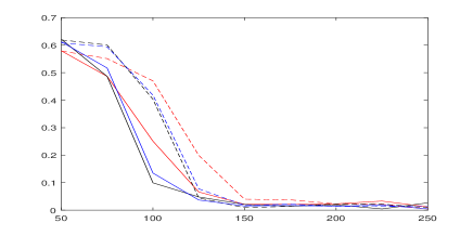
Figure 1: The between-layer clustering errors $R_{BL}$ in (28) of Algorithms 1 (solid lines) and Algorithms 3 (dash lines). Matrices $X^{(m)}$ are generated with $M=3$, $K_{m}=3$, by truncated normal distribution with $\sigma=1$ (left) and the Dirichlet distribution with $\varpi_{k}=\alpha=0.1$, $k\in[K_{m}]$ (right). The entries of $B^{(l)}$ are generated as uniform random numbers between $c=-0.05$ and $d=0.05$. Errors are averaged over 100 simulation runs, $L=50$ (red), $L=100$ (blue), $L=150$ (black).

   

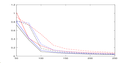
Figure 2: The subspace estimation errors $R_{U,2,\infty}$ in (31) (solid lines) and the errors of spectral embedding (dash lines). Matrices $X^{(m)}$ are generated with $M=3$, $K_{m}=3$, by truncated normal distribution with $\sigma=1$ (left) and the Dirichlet distribution with $\varpi_{k}=\alpha=0.1$, $k\in[K_{m}]$ (right). The entries of $B^{(l)}$ are generated as uniform random numbers between $c=-0.05$ and $d=0.05$. Errors are averaged over 100 simulation runs, $L=50$ (red), $L=100$ (blue), $L=150$ (black).

   

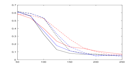
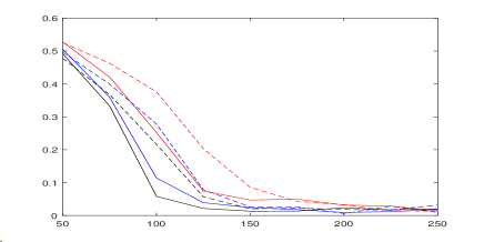
Figure 3: The between-layer clustering errors $R_{BL}$ (left) and the within-layer clustering $R_{WL}$ (right) in (28) and (49), respectively. Layers are equipped with the SBMs where matrices $X^{(m)}$, $m\in[M]$, are generated by the multinomial distributions with probabilities $(1/K_{m},...,1/K_{m})$ with $M=3$ and $K_{m}=3$. The entries of $B^{(l)}$ are generated as uniform random numbers $c=-0.05$ and $d=0.05$. All the non-diagonal entries of those matrices are subsequently multiplied by $w=1$. Errors of Algorithm 1 (solid lines), errors of Algorithms 3 (dash lines). Errors are averaged over 100 simulation runs, $L=50$ (red), $L=100$ (blue), $L=150$ (black).

4.1 4.1  Simulations settings

A limited simulation study, described in this section, has a dual purpose. The first goal is to show that our techniques deliver accurate cluster assignments and ambient subspace estimators in a finite sample case. In particular, we carry out finite sample comparisons with the between-layer clustering in Pensky and Wang (2021). The second goal is to demonstrate advantages of the model itself. Indeed, in many applications, when a network is constructed and edges are drawn, the associated edges’ signs are dropped, and the adjacency matrix has 0/1 entries only. In our simulations examples, we show that by just keeping the sign and allowing the entries of the adjacency matrix take 0/1/-1 values, one can significantly improve the accuracy of the analysis of the network.

In order to attain those objectives, we examine the SGRDPG multiplex networks with matrices $X^{(m)}$, $m\in[M]$, generated by the following three distributions:

Case 1. $f_{m}$ is a truncated normal distribution, so that $\xi\sim f_{m}$ is obtained as $\xi=\eta/\|\eta\|$, where $\eta$ is a $K$-dimensional vector with components being i.i.d. normal with mean zero and variance $\sigma^{2}$.

Case 2. $f_{m}$ is a reduced Dirichlet distribution, so that $\xi\sim f_{m}$ is obtained as the first $K$ components of vector $\eta\in[0,1]^{K+1}$, where $\eta\sim{\rm Dirichlet}(\vec{\varpi})$ with $\vec{\varpi}=(\varpi_{1},...,\varpi_{K+1})$, $\varpi_{k}>0$, $k\in[K+1]$.

Case 3. $f_{m}$ is a the multinomial distribution, so that $\xi\sim f_{m}$ is obtained as $\eta\sim{\rm Multinomial}(\vec{\varpi})$, where $\vec{\varpi}=(\varpi_{1},...,\varpi_{K})$, $0\leq\varpi_{k}\leq 1$, $\varpi_{1}+...+\varpi_{K}=1$. Observe that in this case, distribution $f_{m}$ does not satisfy Assumption A3 and leads to the Signed SBM studied in the Section 3.4.

In order to obtain the DIMPLE-SGRDPG network, we fixed the number of groups of layers $M$ and the ambient dimension of each group of layers $K_{m}$. We generate group membership of each layer $l\in[L]$, using the Multinomial distribution as described in (5) with $\pi_{m}=1/M$. After that, we generate $M$ matrices $X^{(m)}\in[-1,1]^{K_{m}}$ with i.i.d. rows using (6), where $f_{m}$ is one of the three distributions above. Next, we generate the above diagonal entries of symmetric matrices $B^{(l)}$, $l\in[L]$, in (7) as uniform random numbers between $c$ and $d$. Then, connection probability matrices $P^{(l)}$, $l\in[L]$, are of the form (7). The common bases of the ambient subspaces $U^{(m)}$ in groups of layers are formed by the $K$ left singular vectors of matrices $X^{(m)}$, and matrices $Q^{(l)}$ in (3) are of the forms (8). Subsequently, the layer adjacency matrices $A^{(l)}$ are generated according to (2).

4.2 4.2 Simulations results and comparisons with the competitive techniques

Algorithm 3  The between-layer clustering of Pensky and Wang (2021)

Input: Adjacency tensor $\mathbf{A}\in\{0,1\}^{n\times n\times L}$; number of groups of layers $M$; ambient dimension $K^{(l)}$ of each layer $l\in[L]$; parameter $\epsilon$

Output: Estimated clustering clustering function $\hat{s}:[L]\to[M]$ for groups of layers

Steps:
1: Find matrices $\widehat{\widehat{U}}_{A}^{(l)}=SVD_{K^{(l)}}(A^{(l)})$ of $K^{(l)}$ left leading singular vectors of matrices $A^{(l)}$

2: Form matrix $\widetilde{\Theta}\in{\mathbb{R}}^{n^{2}\times L}$ with columns $\widetilde{\Theta}(:,l)=\mbox{vec}(\widehat{\widehat{U}}_{A,l}(\widehat{\widehat{U}}_{A,l})^{T})$, $l\in[L]$

3: Find matrix $\widehat{{\mathcal{W}}}=\mbox{SVD}_{M}(\widetilde{\Theta}^{T})\in{\mathcal{O}}_{L,M}$ of $M$ leading singular vectors of matrix $\widetilde{\Theta}^{T}$

4: Cluster $L$ rows of $\widehat{{\mathcal{W}}}$ into $M$ clusters using $(1+\epsilon)$-approximate $K$-means clustering. Obtain estimated clustering function $\hat{s}$

We obtain the clustering assignment using Algorithm 1, and subsequent ambient subspace estimators using Algorithm 2. Since, to the best of our knowledge, our paper is the first one that studies signed binary networks in the multiplex setting, Algorithm 1 does not have a direct competitor. However, since Pensky and Wang (2021) considered a multiplex network with a similar setting (although without signs), and since their between-layer clustering technique is applicable to the signed setting, we compare our new results with theirs. The between-layer clustering algorithm of Pensky and Wang (2021) is summarized as Algorithm 3 above. Note that estimation of the bases of the ambient subspaces cannot be carried out by the respective algorithm of Pensky and Wang (2021) since the construction of the unbiased tensor of squared averages needs to be modified, due to the presence of signs. Therefore, we shall compare only the between-layer clustering errors of Algorithms 1 and 3.

   

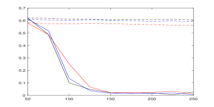
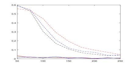
Figure 4: The between-layer clustering errors $R_{BL}$ in (28) of Algorithms 1 with signs (solid lines) and without signs (dash lines). Matrices $X^{(m)}$ are generated by Dirichlet distribution with $M=3$, $K_{m}=K=3$, $\varpi_{k}=\alpha=0.1$, $k\in[K+1]$. The entries of $B^{(l)}$ are generated as uniform random numbers between $c$ and $d$ with $c=-0.05$, $d=0.05$ (left) and $c=-0.2$, $d=0.2$ (right). Errors are averaged over 100 simulation runs, $L=50$ (red), $L=100$ (blue), $L=150$ (black).

   

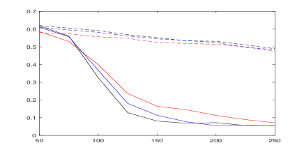
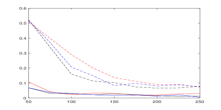
Figure 5: The between-layer clustering errors $R_{BL}$ in (28) of Algorithms 1 with signs (solid lines) and without signs (dash lines). Layers are equipped with the SBMs where matrices $X^{(m)}$. $m\in[M]$, are generated by the multinomial distributions with probabilities $(1/K_{m},...,1/K_{m})$, where $M=3$ and $K_{m}=K=3$. The entries of $B^{(l)}$ are generated as uniform random numbers between $c$ and $d$ with $c=-0.05$, $d=0.05$ (left) and $c=-0.2$, $d=0.2$ (right). All the non-diagonal entries of those matrices are subsequently multiplied by $w=1$. Errors are averaged over 100 simulation runs, $L=50$ (red), $L=100$ (blue), $L=150$ (black).

   

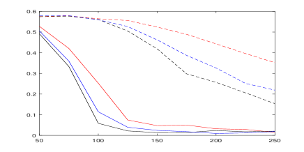
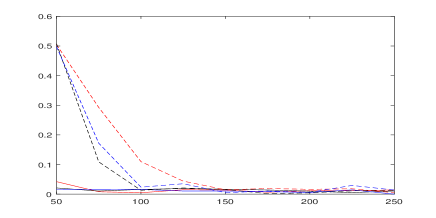
Figure 6: The within-layer clustering errors $R_{WL}$ in (49) with signs (solid lines) and without signs (dash lines). Layers are equipped with the SBMs where matrices $X^{(m)}$. $m\in[M]$, are generated by the multinomial distributions with probabilities $(1/K_{m},...,1/K_{m})$ with $M=3$ and $K_{m}=K=3$. The entries of $B^{(l)}$ are generated as uniform random numbers between $c$ and $d$ with $c=-0.05$, $d=0.05$ (left) and $c=-0.2$, $d=0.2$ (right). All the non-diagonal entries of those matrices are subsequently multiplied by $w=1$. Errors are averaged over 100 simulation runs, $L=50$ (red), $L=100$ (blue), $L=150$ (black).

Two panels of Figure 1 present the between layer clustering errors for Algorithms 1 and 3 when matrices $X^{(m)}$ are generated using truncated normal distribution and the Dirichlet distribution with $M=3$ and $K_{m}=3$. The entries of $B^{(l)}$ are generated as uniform random numbers between $c=-0.05$ and $d=0.05$, so the network is extremely sparse. As Figure 1 demonstrates, even for such a sparse networks the between layer clustering errors are decreasing rapidly, as $n$ grows, and are declining slowly as $L$ increases. It is also obvious from Figure 1 that, although the between layer clustering errors of Algorithm 3 in Pensky and Wang (2021) decrease as $n$ and $L$ grow, they remain larger than the respective errors of Algorithm 1. On the other hand, we should acknowledge that since Algorithms 1 relies on $n$ being somewhat large, Algorithm 3 delivers lesser errors when $n$ is small ($n\leq 40$).

Note that, after the groups of layers are identified, there are two possible ways of estimating the ambient subspaces. The first procedure is summarized in our Algorithm 2. The second approach, the so called spectral embedding, applied in, e.g., Arroyo et al. (2021) and Rubin-Delanchy et al. (2022), consists of placing adjacency matrices $A^{(l)}$ in the same group of layers (with $s(l)=m$) side by side, forming the new matrix $\widehat{H}_{A}^{(m)}\in\{0,1\}^{n\times n\widehat{L}_{m}}$, where $\widehat{L}_{m}$ is the estimated number of layers in a group $m\in[M]$. Afterwards, one estimates $U^{(m)}$ by $\widehat{U}^{(m)}=\mbox{SVD}_{K_{m}}(\widehat{H}_{A}^{(m)})$, the matrix of $K_{m}$ leading singular vectors of $\widehat{H}_{A}^{(m)}$. We described the spectral embedding procedure also in Remark 3.

We compare the subspace estimation errors $R_{U,2,\infty}$ in (31), obtained by Algorithm 2 and by the spectral embedding described above. Results are presented in Figure 2. As it is evident from Figure 2, while the errors of the spectral embedding technique decline as $n$ and $L$ grow, they are still somewhat higher than the errors delivered by Algorithm 2 (unless $n$ is very small), so the technique applied in this paper is somewhat more accurate.

Finally, we compare the accuracy of our Algorithms 1 with the Algorithms 3 of Pensky and Wang (2021) in the situation, where data are generated by the SBM, as it is described in Section 3.4. In this case, we set $K_{m}=K$, $m\in[M]$, and generate group memberships of the layers in exactly the same manner as in all other cases. After that,we generate $M$ matrices $X^{(m)}\in\{0,1\}^{K}$ with i.i.d. rows using the multinomial distribution with equal probabilities $1/K$. Next, we generate the upper triangular entries of symmetric matrices $B^{(l)}$, $l\in[L]$, in (7) as uniform random numbers between $c$ and $d$ and then multiply all the non-diagonal entries of those matrices by $w$. In this manner, if $w<1$ is small, then the network is strongly assortative, i.e., there is a higher probability for nodes in the same community to connect. If $w>1$ is large, then the network is disassortative, i.e., the probability of connection for nodes in different communities is higher than for nodes in the same community. Finally, since entries of matrices $B^{(l)}$ are generated at random, when $w$ is close to one, the networks in all layers are neither assortative or disassortative. Then, connection probability matrices $P^{(l)}$ are of the form (7). Subsequently, the layer adjacency matrices $A^{(l)}$, $l\in[L]$, are generated according to (2).

Similarly to how it was done above, we compare Algorithms 1 with the Algorithms 3 of Pensky and Wang (2021). In addition, we compare the within-layer clustering errors. Since the within-layer clustering methodology of Pensky and Wang (2021) is not designed for signed networks, we apply Algorithm 2 for estimating the ambient subspaces in each group of layers and, subsequently, obtain the community assignment in each group of layers by $(1+\epsilon)$-approximate $K$-means clustering. We measure the accuracy of the community assignment in groups of layers by the average within-layer clustering error given by

$$R_{WL}=\frac{1}{M}\ \min_{\aleph(M)}\ \sum_{m=1}^{M}R_{WL}(m)$$ (49)

$$=\frac{1}{2\,M\,n}\ \min_{\aleph(M)}\ \sum_{m=1}^{M}\left[\min_{\mathscr{P}_{m}\in\mathfrak{F}(K_{m})}\ \|\widehat{\mathbf{Z}}^{(m)}-\mathbf{Z}^{(m)}\,\mathscr{P}_{m}\|^{2}_{F}\right]$$

Results of simulations are presented in Figure 3.

The left panel of Figure 3 confirms that, in the case of the SBM, Algorithms 1 delivers higher accuracy of the between-layer clustering than Algorithms 3. The latter results in the smaller community assignment errors, as it is evident from the right panel of Figure 3.

4.3 4.3  Comparison with the networks where signs are removed

In order to study the effect of removing the signs of the entries of matrices $A^{(l)}$, for each simulation run, we carry out a parallel inference with matrices $P^{(l)}$ and $A^{(l)}$ replaced by $|P^{(l)}|$ and $|A^{(l)}|$, where $|Y|$ denotes the matrix which contains absolute values of the entries of matrix $Y$. We denote the tensors with absolute values, corresponding to $\mathbf{P}$ and $\mathbf{A}$, by $|\mathbf{P}|$ and $|\mathbf{A}|$, respectively.

We consider two examples of the SGRDPG networks, one where the ambient subspaces of the layers of the network are generated using by Dirichlet distribution (Case 2 in Section 4.1), and another, where layers are equipped with the true SBM. The reason for those choices is that, in both cases, it is easy to trace the impact of removing signs on the probability tensor. Specifically, the latter will correspond to removing the signs in the matrices of block probabilities $B^{(l)}$, $l\in[L]$, in (7).

Same as before, in our simulations, we use use Algorithm 1 for clustering layers $A^{(l)}$ and $|A^{(l)}|$, $l\in[L]$, into $M$ groups, and determine the precision of the partition using the between-layer clustering error rate (28). In the case of the SBM, subsequently, we estimate the bases of the ambient subspaces in each of $M$ groups of layers, using Algorithm 2, and cluster the rows by $(1+\epsilon)$-approximate $K$-means clustering, obtaining community assignments for each group of layers. We use the within-layer clustering errors $R_{WL}$ in (49) as a measure of accuracy. Simulations results are presented in Figures 4–6.

It is clear from all three of the figures that the removal of the signs of the edges is extremely detrimental to network analysis. The effects are much more dramatic when a network is extremely sparse (left panels) and are more moderate for denser networks (right panels). Indeed, while the between-layer clustering of the layers is very accurate for $c=-0.05$, $d=0.05$ if edges’ signs are kept, it fails completely when these signs are removed. Moreover, even in the denser case, when $c=-0.2$, $d=0.2$, the differences in clustering precision are very dramatic.

5 5  Real data example

In this section we present application of our model to the brain fMRI data set obtained from the Autism Brain Imaging Data Exchange (ABIDE I) located at
http://fcon 1000.projects.nitrc.org/indi/abide/abide I.html Specifically, we use 37 fMRI brain images obtained by California Institute of Technology and featured in Tyszka et al. (2014). The dataset contains resting-state fMRI data at the whole-brain level of 18 high-functioning adults with an Autism Spectrum Disorders (ASDs) and 19 neurotypical controls with no family history of autism, who were recruited under a protocol approved by the Human Subjects Protection Committee of the California Institute of Technology. The acquisition and initial processing of the data is described in Tyszka et al. (2014), leading to a data matrix of the fMRI recordings over 116 brain regions (see, e.g., Sun et al. (2009)) at 145 time instances.

The goal of our study was to create a signed multilayer network of brain connectivity, with layers being individuals, participating in the study, and to partition the layers of the network into groups using our methodology. For this purpose, we further pre-processed the fMRI signals, using wavelet denoising with the Daubechies-4 wavelets and soft thresholding to reduce noise. Subsequently, we identified 32 brain regions that are related to the ASDs. The necessity of choosing relevant brain regions was motivated by the fact that vast majority of brain regions are not related to cognitive functions and therefore would make partitioning of layers of the network impossible (which was, in essence, the conclusion that Tyszka et al. (2014) drew). Afterwards, for each individual, we created a signed network on the basis of pairwise correlations. Specifically, we used 30% of the highest correlations by absolute value, and created a signed adjacency tensor with values 0,1 and -1. For the sake of comparison, we also created a corresponding adjacency tensor with signs removed.

   

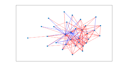
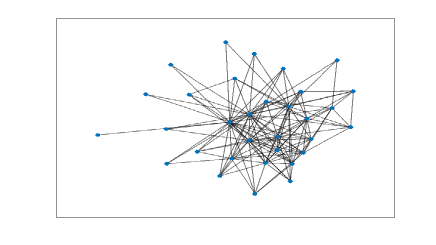
Figure 7: The graph of a network for a brain region with signs (left) and without signs (right). Positive edges are red, negative edges are blue.

   

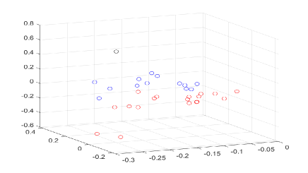
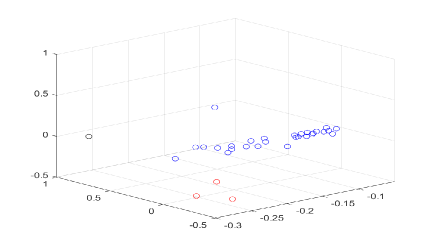
Figure 8: Community assignments in groups of layers of the signed network: group 1 (left), group 2 (right). Nodes in different communities are presented using different colors.

In our analysis, we naturally used $M=2$ (for individuals with and without ASDs), and chose $K=3$. We scrambled the layers of the adjacency tensor and applied Algorithm 3 to its signed and signed-free versions. Since the results of the approximate $k$-means clustering are random, we repeated the process over 100 simulations runs. Thus, we obtained 15.0% average clustering error over signed multilayer network, and 31.2% if we ignore signs (with the standard deviations of about 1.4% in both cases).

Figure 7 pictures a brain network of one of the individuals in th study with signs (left panel) and sign-free (right panel). It is easy to see that negative and positive connections patterns are different, which helps to divide layers of the network into two groups. Specifically, on the average, networks have 144.2 edges with 10.6 edges being negative. If we consider the two groups of layers (individuals with and without ASDs), the average numbers of edges are very similar for the two groups (143.9 for group 1 and 144.3 for group 2), while the average number of negative edges differ (12.9 for group 1 and 8.3 for group 2).

In addition, we analyzed the ambient subspaces for the two groups of layers which are indeed different. Specifically, we evaluated the ambient subspace bases matrices for the two groups $V_{1,S},V_{2,S}$ and $V_{1,NS},V_{2,NS}$, in the signed and sign-free cases, respectively. We evaluated the spectral and the Frobenius $\sin\Theta$ distances, defined in (29), between $V_{1,S}$ and $V_{2,S}$, and also between $V_{1,NS}$ and $V_{2,NS}$. In order to evaluate those results, note that the spectral norms are bounded by one, while the Frobenius norms are bounded by $\sqrt{K}=\sqrt{3}=1.7321$, and the larger values of the norms imply that the subspaces are different. We obtained

$$\begin{array}[]{ll}&\left\|\sin\Theta(V_{1,S},V_{2,S})\right\|=0.9995,\\ &\left\|\sin\Theta(V_{1,S},V_{2,S})\right\|^{2}_{F}=1.3037,\\ &\\ &\left\|\sin\Theta(V_{1,NS},V_{2,NS})\right\|=0.9324,\\ &\left\|\sin\Theta(V_{1,NS},V_{2,NS})\right\|^{2}_{F}=1.2116.\end{array}$$

Further analysis reveals that the first vectors in matrices $V_{1,S},V_{2,S}$ or $V_{1,NS},V_{2,NS}$ are almost identical, while the second and the third are almost orthogonal to each other in the case of the signed network, and have large angles in the case of the network with no signs. Specifically, the acute angles (in degrees) between respective three vectors in $V_{1,S}$ and $V_{2,S}$ are 11.7723^∘, 88.9242^∘ and 72.0369^∘. In the case of the network with no signs, they are 11.4576^∘, 68.0514^∘ and 54.2376^∘. The latter means that the first basis vector is essentially shared by both subspaces, while the second and the third ones are very different and allow to separate layers into two groups. The higher discrepancy between the ambient subspace bases in the case of the signed network leads to the more accurate separation of layers in our example.

Finally, with an additional assumption that layers of the network follow the SBM, we partitioned the nodes in each of the two groups of layers into $K=3$ communities. Figure 8 shows that, under the assumption of the SBM, communities in the two groups are substantially different.

6 6  Proofs

6.1 6.1 Proofs of Lemmas 1 and 2

Proof of Lemma 1.  If $s(l_{1})=m_{1}$ and $s(l_{2})=m_{2}$, then, by (16), one has

$$\Theta(l_{1},l_{2}) =\left[\mbox{vec}\left(\widetilde{U}^{(m_{1})}(\widetilde{U}^{(m_{1})})^{T}\right)\right]^{T}\ \left[\mbox{vec}\left(\widetilde{U}^{(m_{2})}(\widetilde{U}^{(m_{2})}\right)^{T})\right]$$

$$=\|\widetilde{U}^{(m_{1})}(\widetilde{U}^{(m_{2})})^{T}\|^{2}_{F}.$$ (50)

Therefore, if $s(l_{1})=s(l_{2})=m$, then, $\Theta(l_{1},l_{2})=\|\widetilde{U}^{(m)}(\widetilde{U}^{(m)})^{T}\|^{2}_{F}=\|I_{K_{m}}\|^{2}_{F}$, where $I_{k}$ is the identity matrix of size $k$, and (18) holds. If $m_{1}\neq m_{2}$, then, by (21), derive

$$\Theta(l_{1},l_{2})=\frac{\left\|\widetilde{X}^{(m_{1})}\left(\widehat{\Sigma}^{(m_{1})}\right)^{-\frac{1}{2}}\left[\widetilde{X}^{(m_{2})}\left(\widehat{\Sigma}^{(m_{2})}\right)^{-\frac{1}{2}}\right]^{T}\right\|^{2}_{F}}{(n-1)^{2}}.$$ (51)

Then, by Lemma 5, obtain that, if condition (67) holds, then, for $s(l_{1})=m_{1}$ and $s(l_{2})=m_{2}$, with probability at least $1-2\,M\,n^{-\tau}$ one has one has

$$\max_{m_{1}\neq m_{2}}\,|\Theta(l_{1},l_{2})|\leq 4\,\underline{c}^{-2}\,(n-1)^{-2}\,\left\|\widetilde{X}^{(m_{1})}\left(\widetilde{X}^{(m_{2})}\right)^{T}\right\|^{2}_{F}.$$

Application of Lemma 6 and the fact that matrices $\widetilde{X}^{(m)}$ have ranks at most $K$, yield that, with probability at least $1-C\,M\,n^{-\tau}$, one has

$$\max_{l_{1},l_{2}}\,|\Theta(l_{1},l_{2})|\leq C\,K\,n^{-1}\,\log n$$

which completes the proof of (19).

Proof of Lemma 2   Note that, for $l_{1}\neq l_{2}$, one has

$$|(\hat{\theta}^{(l_{1})})^{T}\hat{\theta}^{(l_{2})}-(\theta^{(l_{1})})^{T}\theta^{(l_{2})}| \leq|(\hat{\theta}^{(l_{1})})^{T}[\hat{\theta}^{(l_{2})}-\theta^{(l_{2})}]|$$

$$+|[\hat{\theta}^{(l_{1})}-\theta^{(l_{1})}]^{T}\theta^{(l_{2})}|$$

Since $\|\theta^{(l)}\|^{2}=K_{m}$ for $s(l)=m$, obtain

$$\max_{l_{1},l_{2}}\,|(\hat{\theta}^{(l_{1})})^{T}\hat{\theta}^{(l_{2})}-(\theta^{(l_{1})})^{T}\theta^{(l_{2})}|$$

$$\leq\max_{l\in[L]}\|\hat{\theta}^{(l)}-\theta^{(l)}\|\left[2\sqrt{K_{m}}+\max_{l\in[L]}\|\hat{\theta}^{(l)}-\theta^{(l)}\|\right]$$

Hence, due to

$$\|\hat{\theta}^{(l)}-\theta^{(l)}\| =\left\|\widehat{U}_{A}^{(l)}(\widehat{U}_{A}^{(l)})^{T}-\widetilde{U}_{P}^{(l)}(\widetilde{U}_{P}^{(l)})^{T}\right\|_{F}$$

$$=\sqrt{2}\,\left\|\sin\Theta(\widehat{U}_{A}^{(l)},\widetilde{U}_{P}^{(l)})\right\|_{F}$$

and Lemma 7, derive $|(\hat{\theta}^{(l_{1})})^{T}\hat{\theta}^{(l_{2})}-(\theta^{(l_{1})})^{T}\theta^{(l_{2})}|\leq C\,\sqrt{K}\,(n\rho_{n})^{-1/2}\left[2\sqrt{K}+C\sqrt{K}\,(n\rho_{n})^{-1/2}\right]$, so that

$${\mathbb{P}}\left\{\max_{l_{1},l_{2}}\,|(\hat{\theta}^{(l_{1})})^{T}\hat{\theta}^{(l_{2})}-(\theta^{(l_{1})})^{T}\theta^{(l_{2})}|\leq C\,K\,(n\rho_{n})^{-1/2}\right\}$$

$$\hskip 99.58464pt\geq 1-2n^{-(\tau-\tau_{0})}$$ (52)

Now, observe that, if $s(l_{1})=s(l_{2})=m$, then, due to $K_{m}\geq K/C_{K}$, $\Theta(l_{1},l_{2})=K_{m}$ and $\widehat{\Theta}(l_{1},l_{2})\geq\Theta(l_{1},l_{2})-|(\hat{\theta}^{(l_{1})})^{T}\hat{\theta}^{(l_{2})}-(\theta^{(l_{1})})^{T}\theta^{(l_{2})}|$, one obtains (35) with probability at least $1-2n^{-(\tau-\tau_{0})}$.

In order to derive (36), note that $\widehat{\Theta}(l_{1},l_{2})\leq|\Theta(l_{1},l_{2})|+|(\hat{\theta}^{(l_{1})})^{T}\hat{\theta}^{(l_{2})}-(\theta^{(l_{1})})^{T}\theta^{(l_{2})}|$. Then (36) follows from the combination of (19) and (52) and the fact that $n^{-1}\,\log n=o((n\rho_{n})^{-1/2})$ for large $n$.

6.2 6.2  Proofs of Theorems 1 and 2

Proof of Theorem 1.  Let $Y_{*}=SS^{T}$ where $S$ is the true clustering matrix. Let $\Omega_{\tau}$ be the set of points in the sample space, for which (35) and (36) hold, and let $n$ be large enough, so that, in (35) and (36),

$$\max\left(C_{2}(n\,\rho_{n})^{-1/2},C_{3}K\,(n\,\rho_{n})^{-1/2}\right)<1/2$$ (53)

We need to show that, for $\omega\in\Omega_{\tau}$, for any feasible solution $Y$, one has

$$\langle Y_{*}-Y,\widehat{\Theta}-T\,1_{L}1_{L}^{T}\rangle\geq 0$$ (54)

Note that $Y_{*}(l_{1},l_{2})=I(s(l_{1})=s(l_{2}))$, so that

$$\langle Y_{*}-Y,\widehat{\Theta}-T1_{L}1_{L}^{T}\rangle =\sum_{s(l_{1})=s(l_{2})}\left(1-Y(l_{1},l_{2})\right)\left[T-\widehat{\Theta}(l_{1},l_{2})\right]$$

$$+\sum_{s(l_{1})\neq s(l_{2})}\,Y(l_{1},l_{2})\,\left[T-\widehat{\Theta}(l_{1},l_{2})\right]$$

By conditions of the Theorem and (53), one has $T-\widehat{\Theta}(l_{1},l_{2})\geq 0$ if $s(l_{1})=s(l_{2})$ and $T-\widehat{\Theta}(l_{1},l_{2})\leq 0$ otherwise, since $K_{m}\geq 1$. Then, due to $Y(l_{1},l_{2})\in[0,1]$, obtain (54), which completes the proof.

Proof of Theorem 2   Denote $W=S(S^{T}S)^{-1/2}$, and consider tensors $\mathbf{G}\in{\mathbb{R}}^{n\times n\times L}$ and $\mathbf{H}=\mathbf{G}_{\times 3}W^{T}\in{\mathbb{R}}^{n\times n\times M}$ with layers, respectively, $G^{(l)}=\mathbf{G}(:,:,l)$ and $H^{(m)}=\mathbf{H}(:,:,m)$ of the forms

$$G^{(l)}=(P^{(l)})^{2},\quad H^{(m)}=L_{m}^{-1/2}\,\sum_{s(l)=m}\,G^{(l)}.$$ (55)

Application of the Davis-Kahan theorem yields

$$\left\|\sin\Theta\left(\widehat{U}^{(m)},U^{(m)}\right)\right\|^{2}_{F}\leq\frac{4K\|\widehat{H}^{(m)}-H^{(m)}\|^{2}}{\sigma^{2}_{\min}(H^{(m)})}$$ (56)

Therefore, in order to assess $R_{U,max}$ and $R_{U,ave}$, one needs to examine the spectral structure of matrices $H^{(m)}$ and their deviation from the sample-based versions $\widehat{H}^{(m)}=\widehat{\mathbf{H}}(:,:,m)$. We start with the first task.

It follows from (7) and Assumption A5 that

$$(P^{(l)})^{2}=\rho_{n}^{2}\,X^{(m)}\,B_{0}^{(l)}\,(X^{(m)})^{T}\,X^{(m)}\,B_{0}^{(l)}\,(X^{(m)})^{T}$$ (57)

Recall that, by (12), $X^{(m)}=\widetilde{X}^{(m)}+1_{n}\overline{X}^{(m)}$, where $\widetilde{X}^{(m)}=\Pi^{\bot}X^{(m)}$. Since $(\widetilde{X}^{(m)})^{T}1_{n}\overline{X}^{(m)}=0$, by Lemma 2 of Cai and Zhang [2018a], obtain that $\sigma^{2}_{K_{m}}(X^{(m)})\geq\sigma^{2}_{K_{m}}(\widetilde{X}^{(m)})$. Furthermore, using (20) and Lemma 5, derive

$$\sigma^{2}_{K_{m}}(\widetilde{X}^{(m)})=\lambda_{\min}((\widetilde{X}^{(m)})^{T}\widetilde{X}^{(m)})\geq\underline{c}n/4$$

The latter, together with (57) and Assumption A5, yields $\sigma^{2}_{K_{m}}([P^{(l)}]^{2})\geq\rho_{n}^{2}\,\sigma^{4}_{K_{m}}(\widetilde{X}^{(m)})\,\sigma^{2}_{\min}(B_{0}^{(l)})\geq C\,\rho_{n}^{2}\,n^{2}$. Since matrices $[P^{(l)}]^{2}$ are all positive definite, $\sigma_{K_{m}}(H^{(m)})\geq C\,\sqrt{L_{m}}\,\rho_{n}^{2}\,n^{2}$. Applying Lemma 4 with

$$1+\log(n^{\tau})/\log L\leq t\leq(\underline{c}_{\pi})^{2}\,L/(2M^{2}\log L)-1,$$ (58)

and the union bound, derive from (66) that

$${\mathbb{P}}\left\{\min_{m}\sigma_{K_{m}}(H^{(m)})\geq C\,\sqrt{L/M}\,\rho_{n}^{2}\,n^{2}\right\}\geq 1-2\,n^{-(\tau-\tau_{0})}$$ (59)

Now, we examine deviations $\|\widehat{H}^{(m)}-H^{(m)}\|^{2}$ in (56). Since by Theorem 1, with probability at least $1-C\,n^{-(\tau-\tau_{0})}$ one has $\widehat{W}=W$, by (26), obtain

$$\widehat{H}^{(m)}-H^{(m)}=(\widehat{\mathbf{G}}-\mathbf{G})\times_{3}W^{T}=\frac{1}{\sqrt{L_{m}}}\,\sum_{s(l)=m}[\widehat{G}^{(l)}-G^{(l)}]$$

Now apply Lemma 6 of Noroozi and Pensky [2022] which, in our notations, yields

$${\mathbb{P}}\left\{\|\widehat{H}^{(m)}-H^{(m)}\|^{2}\leq C\left(\rho_{n}^{3}\,n^{3}\,\log(n+L_{m})+\rho_{n}^{2}\,n^{2}\,L_{m}\right)\right\}$$

$$\geq 1-C\,n^{-(\tau-\tau_{0})}-C(n+L_{m})^{-(\tau-1)}$$ (60)

Hence, applying the union bound over $m\in[M]$ in (60) and combining (56), (59), Lemma 4 and (60), we arrive at

$$\left\|\sin\Theta\left(\widehat{U}^{(m)},U^{(m)}\right)\right\|^{2}_{F}\leq C\,\left(\frac{K\,M\,\log n}{\rho_{n}\,n\,L}+\frac{K}{n^{2}}\right)$$ (61)

with probability at least $1-C\,n^{-(\tau-\tau_{0})}-C\,M\,n^{-(\tau-1}$, due to $\log(L_{m}+n)\propto\log(L+n)\propto\log n$. Now, in order the upper bound in (61) holds, one need the condition on $t$ in (58) to be plausible, which is guaranteed by (39) and Assumption A4. The inequality (61) implies that in (33)

$${\mathbb{P}}\,\left\{R_{U,max}\leq C\,\left(\frac{\sqrt{K\,M\,\log n}}{\sqrt{\rho_{n}\,n\,L}}+\frac{\sqrt{K}}{n}\right)\right\}\geq 1-\frac{C}{n^{\tau-\tau_{0}-1}}$$

and that (41) is valid. In order to complete the proof of (40), observe that, with probability at least $1-2\,M\,n^{-\tau}$, one has $\|\widetilde{U}^{(m)}\|_{2,\infty}\leq C\,\sqrt{K/n}$ by (21) and Lemma 5. Application of Lemma 3 completes the proof of (40).

6.3 6.3  Proofs of supplementary statements

Proof of Lemma 3.  First, observe that, for any matrices $A$ and $B$, one has $\|AB\|_{2,\infty}\leq\|A\|\|B\|_{2,\infty}$ and $\|AB\|_{2,\infty}\leq\|A\|_{2,\infty}\|B\|$.

Denote $H=\widehat{U}^{T}U$. Let $H=U_{H}\Lambda_{H}V_{H}^{T}$ be the SVD of $H$. Denote $\widetilde{H}=U_{H}V_{H}^{T}\in{\mathcal{O}}_{K}$. Then,

$$\min_{W\in{\mathcal{O}}_{K}}\|\widehat{U}\,W-U\|_{2,\infty} \leq\|\widehat{U}\,\widetilde{H}-U\|_{2,\infty}\leq\|\widehat{U}(\widetilde{H}-H)\|_{2,\infty}$$

$$+\|\widehat{U}H-U\|_{2,\infty}$$ (62)

Observe that $\Lambda_{H}=\cos(\Theta)$, where $\Theta$ is the diagonal matrix of the principal angles between the subspaces. Therefore,

$$\|H-\widetilde{H}\|=\|U_{H}(\cos\Theta-I_{K})V_{H}^{T}\|=2\|\sin^{2}(\Theta/2)\|\leq\|\sin\Theta\|^{2}$$

due to inequality $\sin(\theta/2)\leq\sin\theta/\sqrt{2}$ for $0\leq\theta\leq\pi/2$. Hence, by Lemma 1 of Cai and Zhang [2018b], one has $\|H-\widetilde{H}\|\leq\epsilon_{1}^{2}$. Since all singular values of $\widetilde{H}$ are equal to one and $\epsilon_{1}\leq 1/2$, derive that $\sigma_{K}(H)\geq 1/2$ and thus $\|H^{-1}\|\leq 2$. Consequently, $\|\widehat{U}\|_{2,\infty}=\|\widehat{U}HH^{-1}\|_{2,\infty}\leq 2\|\widehat{U}H\|_{2,\infty}$ and

$$\|\widehat{U}(\widetilde{H}-H)\|_{2,\infty} \leq 2\|\widehat{U}H\|_{2,\infty}\,\|H-\widetilde{H}\|$$

$$\leq 2\epsilon_{1}^{2}(\|\widehat{U}H-U\|_{2,\infty}+\|U\|_{2,\infty}).$$ (63)

Now, notice that

$$\|\widehat{U}H-U\|_{2,\infty} =\|\widehat{U}\widehat{U}^{T}U-UU^{T}U\|_{2,\infty}$$ (64)

$$\leq\|\widehat{U}\widehat{U}^{T}-UU^{T}\|\,\|U\|_{2,\infty}\leq\epsilon_{1}\epsilon_{2},$$

which, together with (63), implies that $\|\widehat{U}(\widetilde{H}-H)\|_{2,\infty}\leq 2\epsilon_{1}^{2}(\epsilon_{1}\epsilon_{2}+\epsilon_{2})$. Plugging the latter and (64) into (62) and recalling that $\epsilon_{1}\leq 1/2$, obtain (43)

Lemma 4.

Let Assumption A1 hold. Denote

$$L_{m}=\sum_{l=1}^{M}I(s(l)=m),\quad m\in[M]$$ (65)

If $t\leq(\underline{c}_{\pi})^{2}\,L/(2M^{2}\log L)-1$, then,

$${\mathbb{P}}\left\{\bigcap_{m=1}^{M}\,\left(\frac{\underline{c}_{\pi}\,L}{2\,M}\leq L_{m}\leq\frac{3\,\bar{c}_{\pi}\ L}{2\,M}\right)\right\}\geq 1-2L^{-t}$$ (66)

Proof of Lemma 4.  Note that $L_{m}\sim\text{Binomial}(\pi_{m},L)$ for a fixed $m$. By Hoeffding inequality, for any $x>0$

$${\mathbb{P}}\left\{\left|L_{m}/L-\pi_{m}\right|\geq x\right\}\leq 2\exp\{-2Lx^{2}\}$$

Then, applying Assumption A1 and the union bound, obtain

$${\mathbb{P}}\left\{\bigcap_{m=1}^{M}\,\left(\underline{c}_{\pi}\,L/M-Lx\leq L_{m}\leq\bar{c}_{\pi}\,\,L/M+Lx\right)\right\}$$

$$\geq 1-2M\,\exp\{-2Lx^{2}\}$$

Now, set $x=\sqrt{\log(L^{t}\,M)/(2L)}$, which is equivalent to $M\,\exp\{-2Lx^{2}\}=L^{-t}$. If let $L$ is large enough, so that $x<\underline{c}_{\pi}/(2\,M)$, then (66) holds. The latter is guaranteed by $t+1\leq(\underline{c}_{\pi})^{2}\,L/(2M^{2}\log L)$.

Lemma 5.

Let Assumptions A1–A4 hold. Let $n$ be large enough, so that

$$n\geq 2\,(C_{\tau})^{2}\,(\bar{c})^{2}\,(\underline{c})^{-4}\,(K+\tau\log n)$$ (67)

where $C_{\tau}$ is the constant in (69) Then, for any fixed constant $\tau$, one has

$${\mathbb{P}}\left\{\min_{m\in[M]}\ \lambda_{\min}(\widehat{\Sigma}^{(m)})\geq\frac{\underline{c}}{2}\right\}\geq 1-2\,M\,n^{-\tau}$$ (68)

Proof of Lemma 5.  Apply Theorem 6.5 of Wainwright [2019] which states that, under conditions of the Lemma

$${\mathbb{P}}\left\{\|\widehat{\Sigma}^{(m)}-\Sigma^{(m)}\|\leq\frac{C_{\tau}\,\bar{c}}{\underline{c}}\,\sqrt{\frac{K+\tau\log n}{n}}\right\}\geq 1-2\,n^{-\tau}$$ (69)

Since $\lambda_{\min}(\widehat{\Sigma}^{(m)})\geq\lambda_{\min}(\Sigma^{(m)})-\|\widehat{\Sigma}^{(m)}-\Sigma^{(m)}\|$, by Assumption A3, obtain that

$${\mathbb{P}}\left\{\lambda_{\min}(\widehat{\Sigma}^{(m)})\geq\underline{c}\left[1-\frac{C_{\tau}\,\bar{c}}{\underline{c}^{2}}\,\sqrt{\frac{K+\tau\log n}{n}}\right]\right\}\geq 1-\frac{2}{n^{\tau}}$$ (70)

If $n$ satisfies (67), the expression in the square brackets in (70) is bounded below by 1/2 and, by taking the union bound in (70), we complete the proof.

Lemma 6.

Let Assumptions A1–A4 hold. Then, for any fixed constant $\tau$, one has

$${\mathbb{P}}\left\{\max_{i\neq j}\ \|(\widetilde{X}^{(i)})^{T}\,\widetilde{X}^{(j)}\|\leq C_{1}\,\sqrt{n\,\log n}\right\}\geq 1-C_{2}\,n^{-\tau}$$ (71)

where $C_{1}$ and $C_{2}$ in (71) depend on $\tau$ and constants in Assumptions A1–A4 only.

Proof of Lemma 6.  Note that $\widetilde{X}^{(i)}=X^{(i)}-\Pi X^{(i)}=(X^{(i)}-1_{n}\mu^{(i)})+(1_{n}\mu^{(i)}-\Pi X^{(i)})$. Introduce matrices

$$\xi^{(i)}=X^{(i)}-1_{n}\mu^{(m_{i})},\quad\eta^{(i)}=1_{n}\mu^{(i)}-\Pi X^{(i)},$$ (72)

$$\xi^{(i)},\eta^{(i)}\in{\mathbb{R}}^{n\times K_{i}},\ \ i\in[M]$$

Observe that, by (6), one has ${\mathbb{E}}\xi^{(i)}={\mathbb{E}}\eta^{(i)}=0$ and that pairs $(\xi^{(i)},\eta^{(i)})$ and $(\xi^{(j)},\eta^{(j)})$ are independent for $i\neq j$. Note also that

$$\Delta^{(i,j)}=\|(\widetilde{X}^{(i)})^{T}\,\widetilde{X}^{(j)}\|\leq\Delta_{1}^{(i,j)}+\Delta_{2}^{(i,j)}+\Delta_{3}^{(i,j)}+\Delta_{4}^{(i,j)}$$ (73)

where $\Delta_{1}^{(i,j)}=\|(\xi^{(i)})^{T}\xi^{(j)}\|$, $\Delta_{2}^{(i,j)}=\|(\xi^{(i)})^{T}\eta^{(j)}\|$, $\Delta_{3}^{(i,j)}=\|(\eta^{(i)})^{T}\xi^{(j)}\|$ and $\Delta_{4}^{(i,j)}=\|(\eta^{(i)})^{T}\eta^{(j)}\|$. Below, we construct upper bounds for $\Delta_{k}$, $k=1,2,3,4$.

An upper bound for $\Delta_{1}^{(i,j)}$.  Consider matrix $\Psi=(\xi^{(i)})^{T}\xi^{(j)}\in{\mathbb{R}}^{K_{i}\times K_{j}}$ and notice that

$$\Psi=\sum_{t=1}^{n}\Psi_{t},\quad\Psi_{t}=(\xi^{(i)}(t,:))^{T}\,\xi^{(j)}(t,:),\quad{\mathbb{E}}\Psi_{t}=0,$$

where rank one matrices $\Psi_{t}$ are i.i.d. for different values of $t\in[n]$. We apply matrix Bernstein inequality from Tropp [2011]

$${\mathbb{P}}\left\{\|\Psi\|\geq z\right\}\leq(K_{i}+K_{j})\,\exp\left\{-\frac{z^{2}}{2(n\,\delta_{1}+z\,\delta_{2}/3)}\right\}$$ (74)

where $\delta_{1}=\max\left[\|{\mathbb{E}}(\Psi_{1}\Psi_{1}^{T})\|,\|{\mathbb{E}}(\Psi_{1}^{T}\Psi_{1})\|\right]$ and $\delta_{2}=\displaystyle\max_{t}\|\Psi_{t}\|$. It is easy to see that $\delta_{2}=\|\xi^{(i)}(t,:)\|\|\xi^{(j)}(t,:)\|\leq 1$ by Assumption A2. In order to upper-bound $\delta_{1}$, note that

$${\mathbb{E}}(\Psi_{1}\Psi_{1}^{T}) ={\mathbb{E}}\|\xi^{(j)}(t,:)\|^{2}\,{\mathbb{E}}\left[(\xi^{(i)}(1,:))^{T}\,\xi^{(i)}(1,:)\right]$$

$$\leq{\mathbb{E}}\left[(\xi^{(i)}(1,:))^{T}\,\xi^{(i)}(1,:)\right]$$

and, by (6), ${\mathbb{E}}\left[(\xi^{(i)}(1,:))^{T}\,\xi^{(i)}(1,:)\right]=\Sigma^{(i)}$. Therefore, $\|{\mathbb{E}}(\Psi_{1}\Psi_{1}^{T})\|\leq\bar{c}$. Similarly,

$${\mathbb{E}}(\Psi_{1}^{T}\Psi_{1}) ={\mathbb{E}}\left[\xi^{(i)}(1,:)\,{\mathbb{E}}\left((\xi^{(j)}(1,:))^{T}\,\xi^{(j)}(1,:)\right)(\xi^{(i)}(1,:))^{T}\right]$$

$$={\mathbb{E}}\left[\xi^{(i)}(1,:)\,\Sigma^{(i)}(\xi^{(i)}(1,:))^{T}\right]\$$

and, hence

$$\|{\mathbb{E}}(\Psi_{1}^{T}\Psi_{1})\|\leq\bar{c}\,{\mathbb{E}}\|\xi^{(i)}(1,:)\|^{2}\leq\bar{c}$$

Therefore, combination of (74) and the union bound over $i,j\in[M]$ yield, for any $\tau>0$,

$${\mathbb{P}}\left\{\max_{i\neq j}\ \Delta_{1}^{(i,j)}\leq C\,\sqrt{n\,\log(M^{2}\,n)}\right\}\geq 1-n^{-\tau}$$ (75)

Now, consider $\Delta_{2}^{(i,j)}=\|(\xi^{(i)})^{T}\eta^{(j)}\|$. Observe that, due to $n^{-1}1_{n}^{T}X^{(i)}=\overline{X}^{(i)}$, one has

$$(\xi^{(i)})^{T}\eta^{(j)} =(X^{(i)}-1_{n}\mu^{(m_{i})})^{T}(1_{n}\mu^{(j)}-\Pi X^{(j)})$$

$$=n(\overline{X}^{(i)}-\mu^{(i)})^{T}(\overline{X}^{(j)}-\mu^{(j)}).$$

and a similar calculation applies to $(\eta^{(i)})^{T}\xi^{(j)}$ and $(\eta^{(i)})^{T}\eta^{(j)}$. Therefore, for $i,j\in[M]$

$$\Delta_{k}^{(i,j)}\leq n\,\|\overline{X}^{(i)}-\mu^{(i)}\|\,\|\overline{X}^{(j)}-\mu^{(j)}\|,\quad k=2,3,4.$$ (76)

It is known (see, e.g., Wainwright [2019]) that if $\zeta$ is a zero mean sub-gaussian $k$-dimensional random vector with the sub-gaussian parameter $\sigma$, then

$${\mathbb{P}}\left\{\|\zeta\|\leq 4\sigma\sqrt{k}+2\sigma\sqrt{\log(1/\epsilon)}\right\}\geq 1-\epsilon$$ (77)

Note that vectors $(\Sigma^{(i)})^{-1/2}\,(X(j,:)-\mu^{(i)})$ are anisotropic $K_{i}$ dimensional random vectors of length at most $1/\sqrt{\underline{c}}$. Hence, vectors $(\Sigma^{(i)})^{-1/2}\,(\overline{X}^{(i)}-\mu^{(i)})$ are anisotropic sub-gaussian with $\sigma\leq 2/\sqrt{\underline{c}\,n}$, so that

$${\mathbb{P}}\left\{\|\overline{X}^{(i)}-\mu^{(i)}\|\leq\frac{4\sqrt{\bar{c}}[2\,\sqrt{K}+\sqrt{\log(M^{2}\,n^{\tau})}]}{\sqrt{n\,\underline{c}}}\right\}\geq 1-\frac{1}{M^{2}n^{\tau}}$$ (78)

Combining (76), (78) and the union bound over $i,j\in[M]$, $i\neq j$, obtain, fpr $k=2,3,4$:

$${\mathbb{P}}\left\{\max_{i\neq j}\ \Delta_{k}^{(i,j)}\leq C\,\sqrt{K+\log(M^{2}\,n)}\right\}\geq 1-n^{-\tau},$$ (79)

which, together with (75) and $\log(M^{2}\,n)\propto\log n$, complete the proof.

Lemma 7.

Let Assumptions A1–A5 and (34) hold. Then, if $n$ is large enough, for any fixed constant $\tau$, one has

$${\mathbb{P}}\left\{\max_{l\in[L]}\,\left\|\sin\Theta(\widehat{U}_{A}^{(l)},\widetilde{U}_{P}^{(l)})\right\|_{F}\leq\frac{C\sqrt{K}}{\sqrt{n\rho_{n}}}\right\}\geq 1-\frac{2}{n^{\tau-\tau_{0}}}$$ (80)

Proof of Lemma 7.  It follows from Le et al. [2018] that, under condition (34), one has

$${\mathbb{E}}\|A^{(l)}-P^{(l)}\|\leq C\left(\sqrt{n\rho_{n}}+\sqrt{\log n}\right)$$

Also, by formula (2.4) of Benaych-Georges et al. [2020], derive that, for any $t>0$, and some absolute constant $\widetilde{C}$ one has

$${\mathbb{P}}\left\{\|A^{(l)}-P^{(l)}\|-{\mathbb{E}}\|A^{(l)}-P^{(l)}\|\geq t\right\}\leq 2\,\exp(-\widetilde{C}\,t^{2})$$

Setting $t=\sqrt{\widetilde{C}^{-1}\,\log(n^{\tau}\,L)}$, combining the two inequalities above and applying the union bound, obtain

$${\mathbb{P}}\left\{\|A^{(l)}-P^{(l)}\|\leq C\left(\sqrt{n\rho_{n}}+\sqrt{\log(n^{\tau}\,L)}\right)\right\}\geq 1-\frac{2}{n^{\tau}},$$ (81)

where the constant $C$ in (81) depends on $\tau$ and the constants in Assumptions A1–A5. Taking into account that $\|\widetilde{A}^{(l)}-\widetilde{P}^{(l)}\|\leq\|A^{(l)}-P^{(l)}\|$ and that, under assumptions of the Lemma, $\log(n^{\tau}\,L)\leq C\log n\leq Cn\rho_{n}$, derive that

$${\mathbb{P}}\left\{\|\widetilde{A}^{(l)}-\widetilde{P}^{(l)}\|\leq C\sqrt{n\rho_{n}}\right\}\geq 1-2\,n^{-\tau}$$ (82)

By Davis-Kahan Theorem (see, e.g., Yu et al. [2014]), if $s(l)=m$, obtain

$$\left\|\sin\Theta(\widehat{U}_{A}^{(l)},\widetilde{U}_{P}^{(l)})\right\|_{F}\leq\frac{2\,\sqrt{K_{m}}\|\widetilde{A}^{(l)}-\widetilde{P}^{(l)}\|}{\sigma_{K_{m}}(\widetilde{P}^{(l)})}$$ (83)

Here, by (13) and (14), $\widetilde{P}^{(l)}=\widetilde{X}^{(m)}B^{(l)}(\widetilde{X}^{(m)})^{T}=\rho_{n}\,\widetilde{U}^{(m)}\widetilde{D}^{(m)}(\widetilde{O}^{(m)})^{T}B_{0}^{(l)}(\widetilde{D}^{(m)}(\widetilde{O}^{(m)})^{T})^{T}(\widetilde{U}^{(m)})^{T}$, so that, by (20), $\widetilde{P}^{(l)}=(n-1)\,\rho_{n}\,\widetilde{U}^{(m)}\sqrt{\widehat{\Sigma}^{(m)}}\,B_{0}^{(l)}\,(\sqrt{\widehat{\Sigma}^{(m)}})^{T}\,(\widetilde{U}^{(m)})^{T}$. Therefore, Assumption A5 and Lemma 5 imply that

$$\sigma_{K_{m}}(\widetilde{P}^{(l)})\geq Cn\rho_{n}$$

Combining the latter with (82) and (83), using the union bound over $l\in[L]$, and taking into account that $K_{m}\leq K$, obtain (80).

References

• Agterberg and Zhang [2022] J. Agterberg and A. Zhang. Estimating higher-order mixed memberships via the $\ell_{2,\infty}$ tensor perturbation bound. ArXiv: 2212.08642, 2022.
• Agterberg et al. [2022] J. Agterberg, Z. Lubberts, and J. Arroyo. Joint spectral clustering in multilayer degree-corrected stochastic blockmodels. ArXiv: 2212.05053, 2022.
• Airoldi et al. [2008] E. M. Airoldi, D. M. Blei, S. E. Fienberg, and E. P. Xing. Mixed membership stochastic blockmodels. J. Mach. Learn. Res., 9:1981–2014, June 2008. ISSN 1532-4435.
• Arroyo et al. [2021] J. Arroyo, A. Athreya, J. Cape, G. Chen, C. E. Priebe, and J. T. Vogelstein. Inference for multiple heterogeneous networks with a common invariant subspace. Journal of Machine Learning Research, 22(142):1–49, 2021. URL http://jmlr.org/papers/v22/19-558.html.
• Athreya et al. [2018] A. Athreya, D. E. Fishkind, M. Tang, C. E. Priebe, Y. Park, J. T. Vogelstein, K. Levin, V. Lyzinski, Y. Qin, and D. L. Sussman. Statistical inference on random dot product graphs: a survey. Journal of Machine Learning Research, 18(226):1–92, 2018. URL http://jmlr.org/papers/v18/17-448.html.
• Athreya et al. [2022] A. Athreya, Z. Lubberts, Y. Park, and C. E. Priebe. Discovering underlying dynamics in time series of networks. ArXiv: 2205.06877, 2022. 10.48550/ARXIV.2205.06877.
• Babul and Lambiotte [2023] S. Babul and R. Lambiotte. Sheep: Signed hamiltonian eigenvector embedding for proximity. ArXiv:2302.07129, 2023.
• Benaych-Georges et al. [2020] F. Benaych-Georges, C. Bordenave, and A. Knowles. Spectral radii of sparse random matrices. Annales de l’Institut Henri Poincaré, Probabilités et Statistiques, 56(3):2141 – 2161, 2020. 10.1214/19-AIHP1033. URL https://doi.org/10.1214/19-AIHP1033.
• Cai and Zhang [2018a] T. T. Cai and A. Zhang. Rate-optimal perturbation bounds for singular subspaces with applications to high-dimensional statistics. The Annals of Statistics, 46(1):60 – 89, 2018a. 10.1214/17-AOS1541. URL https://doi.org/10.1214/17-AOS1541.
• Cai and Zhang [2018b] T. T. Cai and A. Zhang. Rate-optimal perturbation bounds for singular subspaces with applications to high-dimensional statistics. Ann. Statist., 46(1):60–89, 02 2018b. 10.1214/17-AOS1541. URL https://doi.org/10.1214/17-AOS1541.
• Cheng et al. [2017] J. Cheng, T. Li, E. Levina, and J. Zhu. High-dimensional mixed graphical models. Journal of Computational and Graphical Statistics, 26(2):367–378, 2017.
• Chi et al. [2020] E. C. Chi, B. J. Gaines, W. W. Sun, H. Zhou, and J. Yang. Provable convex co-clustering of tensors. Journal of Machine Learning Research, 21(214):1–58, 2020. URL http://jmlr.org/papers/v21/18-155.html.
• Cucuringu et al. [2019] M. Cucuringu, D. P., G. A., and H. Tyagi. SPONGE: A generalized eigenproblem for clustering signed networks. AISTATS, 2019.
• Davis [1967] J. A. Davis. Clustering and structural balance in graphs. Human relations, 20(2):181–187, 1967.
• De Domenico et al. [2015] M. De Domenico, V. Nicosia, A. Arenas, and V. Latora. Structural reducibility of multilayer networks. Nature Communications, 6(6864), 2015. doi:10.1038/ncomms7864.
• Donoho et al. [2023] D. Donoho, M. Gavish, and E. Romanov. ScreeNOT: Exact MSE-optimal singular value thresholding in correlated noise. The Annals of Statistics, 51(1):122 – 148, 2023. 10.1214/22-AOS2232. URL https://doi.org/10.1214/22-AOS2232.
• Estrada and Benzi [2014] E. Estrada and M. Benzi. A walk-based measure of balance in signed networks. detecting lack of balance in social networks. Physical Review E, 90:#042802, 2014.
• Fan et al. [2022] X. Fan, M. Pensky, F. Yu, and T. Zhang. Alma: Alternating minimization algorithm for clustering mixture multilayer network. Journal of Machine Learning Research, 23(330):1–46, 2022. URL http://jmlr.org/papers/v23/21-0182.html.
• Feng et al. [2022] D. Feng, R. Altmeyer, D. Stafford, N. A. Christakis, and H. H. Zhou. Testing for Balance in Social Networks. Journal of the American Statistical Association, 117(537):156–174, January 2022. 10.1080/01621459.2020.176. URL https://ideas.repec.org/a/taf/jnlasa/v117y2022i537p156-174.html.
• Gallagher et al. [2023+] I. Gallagher, A. Jones, A. Bertiger, C. E. Priebe, and P. Rubin-Delanchy. Spectral embedding of weighted graphs. Journal of the American Statistical Association, 0(0):1–10, 2023+. 10.1080/01621459.2023.2225239. URL https://doi.org/10.1080/01621459.2023.2225239.
• Gallo et al. [2023] A. Gallo, D. Garlaschelli, R. Lambiotte, F. Saracco, and T. Squartini. Strong, weak or no balance? testing structural hypotheses in real heterogeneous networks. ArXiv:2303.07023, 2023.
• Gao et al. [2017] C. Gao, Z. Ma, A. Y. Zhang, and H. H. Zhou. Achieving optimal misclassification proportion in stochastic block models. J. Mach. Learn. Res., 18(1):1980–2024, Jan. 2017. ISSN 1532-4435.
• Gao et al. [2018] C. Gao, Z. Ma, A. Y. Zhang, and H. H. Zhou. Community detection in degree-corrected block models. Ann. Statist., 46(5):2153–2185, 10 2018. 10.1214/17-AOS1615.
• Gartner and Matousek [2012] B. Gartner and J. Matousek. Approximation Algorithms and Semidefinite Programming. Springer Publishing Company, 2012. ISBN 038788145X, 9780387881454. DOI10.1007/978-3-642-22015-9.
• Han et al. [2022] R. Han, Y. Luo, M. Wang, and A. R. Zhang. Exact clustering in tensor block model: Statistical optimality and computational limit. Journal of the Royal Statistical Society Series B, 84(5):1666–1698, November 2022. 10.1111/rssb.12547.
• Harary [1953] F. Harary. On the notion of balance of a signed graph. Michigan Mathematical Journal, 2(2):143 – 146, 1953. 10.1307/mmj/1028989917. URL https://doi.org/10.1307/mmj/1028989917.
• Jing et al. [2021] B.-Y. Jing, T. Li, Z. Lyu, and D. Xia. Community detection on mixture multilayer networks via regularized tensor decomposition. The Annals of Statistics, 49(6):3181 – 3205, 2021. 10.1214/21-AOS2079. URL https://doi.org/10.1214/21-AOS2079.
• Jones and Rubin-Delanchy [2020] A. Jones and P. Rubin-Delanchy. The multilayer random dot product graph. ArXiv: 2007.10455, 2020. 10.48550/ARXIV.2007.10455.
• Ke and Wang [2022] Z. T. Ke and J. Wang. Optimal network membership estimation under severe degree heterogeneity. ArXiv:2204.12087, 2022.
• Kirkley et al. [2019] A. Kirkley, G. T. Cantwell, and M. E. J. Newman. Balance in signed networks. Physical Review E, 99:#012320, 2019. 10.1103/PhysRevE.99.012320. URL https://link.aps.org/doi/10.1103/PhysRevE.99.012320.
• Kivela et al. [2014] M. Kivela, A. Arenas, M. Barthelemy, J. P. Gleeson, Y. Moreno, and M. A. Porter. Multilayer networks. Journal of Complex Networks, 2(3):203–271, 07 2014. ISSN 2051-1329. 10.1093/comnet/cnu016. URL https://doi.org/10.1093/comnet/cnu016.
• Koo et al. [2022] J. Koo, M. Tang, and M. W. Trosset. Popularity adjusted block models are generalized random dot product graphs. Journal of Computational and Graphical Statistics, 0(0):1–14, 2022. 10.1080/10618600.2022.2081576. URL https://doi.org/10.1080/10618600.2022.2081576.
• Le and Levina [2015] C. M. Le and E. Levina. Estimating the number of communities in networks by spectral methods. ArXiv:1507.00827, 2015.
• Le et al. [2018] C. M. Le, E. Levina, and R. Vershynin. Concentration of random graphs and application to community detection, pages 2925–2943. ICM, 2018. 10.1142/9789813272880_0166.
• Levin et al. [2022] K. Levin, A. Lodhia, and E. Levina. Recovering shared structure from multiple networks with unknown edge distributions. J. Mach. Learn. Res., 23(1), 2022. ISSN 1532-4435.
• Luo et al. [2021] Y. Luo, G. Raskutti, M. Yuan, and A. R. Zhang. A sharp blockwise tensor perturbation bound for orthogonal iteration. Journal of Machine Learning Research, 22(179):1–48, 2021. URL http://jmlr.org/papers/v22/20-919.html.
• MacDonald et al. [2021] P. W. MacDonald, E. Levina, and J. Zhu. Latent space models for multiplex networks with shared structure. ArXiv: 2012.14409, 2021.
• Noroozi and Pensky [2022] M. Noroozi and M. Pensky. Sparse subspace clustering in diverse multiplex network model. arXiv preprint arXiv:2206.07602, 2022.
• Noroozi et al. [2021] M. Noroozi, R. Rimal, and M. Pensky. Estimation and clustering in popularity adjusted block model. Journal of The Royal Statistical Society Series B-statistical Methodology, 83:293–317, 2021.
• Pensky and Wang [2021] M. Pensky and Y. Wang. Clustering of diverse multiplex networks. arXiv preprint arXiv:2110.05308, 2021.
• Rubin-Delanchy et al. [2022] P. Rubin-Delanchy, J. Cape, M. Tang, and C. E. Priebe. A Statistical Interpretation of Spectral Embedding: The Generalised Random Dot Product Graph. Journal of the Royal Statistical Society Series B: Statistical Methodology, 84(4):1446–1473, 06 2022. ISSN 1369-7412. 10.1111/rssb.12509. URL https://doi.org/10.1111/rssb.12509.
• Singh and Adhikari [2017] R. Singh and B. Adhikari. Measuring the balance of signed networks and its application to sign prediction. Journal of Statistical Mechanics: Theory and Experiment, 2017(6):063302, jun 2017. 10.1088/1742-5468/aa73ef. URL https://dx.doi.org/10.1088/1742-5468/aa73ef.
• Sporns [2018] O. Sporns. Graph theory methods: applications in brain networks. Dialogues in Clinical Neuroscience, 20(2):111–121, 2018.
• Sun et al. [2009] L. Sun, R. Patel, J. Liu, K. Chen, T. Wu, J. Li, E. M. Reiman, and J. Ye. Mining brain region connectivity for alzheimer’s disease study via sparse inverse covariance estimation. In Knowledge Discovery and Data Mining, 2009. URL https://api.semanticscholar.org/CorpusID:7857678.
• Tropp [2011] J. A. Tropp. User-friendly tail bounds for sums of random matrices. Foundations of Computational Mathematics, 12(4):389–434, 2011.
• Tyszka et al. [2014] J. M. Tyszka, D. P. Kennedy, L. K. Paul, and R. Adolphs. Largely typical patterns of resting-state functional connectivity in high-functioning adults with autism. Cerebral Cortex, 24(7):1894–1905, Jul 2014. ISSN 1047-3211.
• Wainwright [2019] M. J. Wainwright. High-Dimensional Statistics: A Non-Asymptotic Viewpoint. Cambridge Series in Statistical and Probabilistic Mathematics. Cambridge University Press, 2019. 10.1017/9781108627771.
• Yu et al. [2014] Y. Yu, T. Wang, and R. J. Samworth. A useful variant of the davis-kahan theorem for statisticians. Biometrika, 102(2):315–323, 04 2014. ISSN 0006-3444. 10.1093/biomet/asv008. URL https://doi.org/10.1093/biomet/asv008.
• Zhang and Xia [2018] A. Zhang and D. Xia. Tensor svd: Statistical and computational limits. IEEE Transactions on Information Theory, 64(11):7311–7338, 2018. 10.1109/TIT.2018.2841377.
• Zhang et al. [2012] T. Zhang, A. Szlam, Y. Wang, and G. Lerman. Hybrid linear modeling via local best-fit flats. International Journal of Computer Vision, 100(3):217–240, Dec 2012. ISSN 1573-1405. 10.1007/s11263-012-0535-6. URL https://doi.org/10.1007/s11263-012-0535-6.
• Zheng and Tang [2022] R. Zheng and M. Tang. Limit results for distributed estimation of invariant subspaces in multiple networks inference and pca. ArXiv: 2206.04306, 2022. 10.48550/ARXIV.2206.04306.