Ising on the Graph: Task-specific Graph Subsampling via the Ising Model

Abstract

Reducing a graph while preserving its overall structure is an important problem with many applications. Typically, the reduction approaches either remove edges (sparsification) or merge nodes (coarsening) in an unsupervised way with no specific downstream task in mind. In this paper, we present an approach for subsampling graph structures using an Ising model defined on either the nodes or edges and learning the external magnetic field of the Ising model using a graph neural network. Our approach is task-specific as it can learn how to reduce a graph for a specific downstream task in an end-to-end fashion. The utilized loss function of the task does not even have to be differentiable. We showcase the versatility of our approach on three distinct applications: image segmentation, 3D shape sparsification, and sparse approximate matrix inverse determination.

1 Introduction

Hierarchical organization is a recurring theme in nature and human endeavors (Pumain, 2006). Part of its appeal lies in the interpretability and computational efficiency it affords, especially on uniformly discretized domains such as images or time series (Duhamel & Vetterli, 1990; Mallat, 1999; Hackbusch, 2013; Lindeberg, 2013). On graph-structured data, it is, however, no longer as clear what it means to, e.g., “sample every second point” as shown in Figure 1. Solid theoretical arguments favor a spectral approach (Shuman et al., 2015), wherein a simplified graph is found by maximizing the spectral similarity of the original graph (Jin et al., 2020). On the other hand, instead of retaining as much of the original information as possible, it may often be more valuable to distill the critical information for the task at hand (Cai et al., 2021; Jin et al., 2022a). The two main approaches for graph simplification, coarsening, and sparsification, involve removing nodes and edges, respectively. However, using existing methods, it is not possible to tailor coarsening or sparsification to a particular task.

We take inspiration from the well-known Ising model in physics (Cipra, 1987), which emanated as an analytical tool for studying magnetism but has since undergone many extensions (Wu, 1982; Nishimori, 2001). Within the Ising model, each location is associated with a binary state (interpreted as pointing up or down), and the configuration of all states is associated with an energy.

Thus, the Ising model can be seen as an energy-based model with an energy function comprising a pairwise term and a pointwise “bias” term. As illustrated in Figure 2, the sign of the pairwise term determines whether neighboring states attract or repel each other, while the pointwise term (corresponding to the local magnetic field) controls the propensity of a particular alignment.

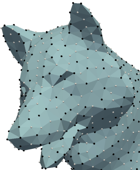
Figure 1: Sampled vertices using the Ising model with a learned magnetic field. Black vertices are retained in the coarse mesh and define the general shape, while white vertices only add details.

In this paper, we consider the Ising model defined on either the nodes or the edges of a graph and augment it with a graph neural network that models the local magnetic field. There are no particular restrictions on the type of graph neural network, which means that it can, e.g., process multidimensional node and edge features. Since choosing whether to include a node (or edge) is binary, we use techniques for gradient estimation in discrete models to train our model for a given task. Specifically, we show that the two-point version of the REINFORCE Leave-One-Out estimator (e.g., Shi et al. (2022)) results in a straightforward expression and allows for using non-differentiable task-specific losses. To showcase the broad applicability of our model, we demonstrate how it can be used in several domains: image segmentation, 3D shape sparsification, and linear algebra (sparse approximate inverse determination).

2 Background

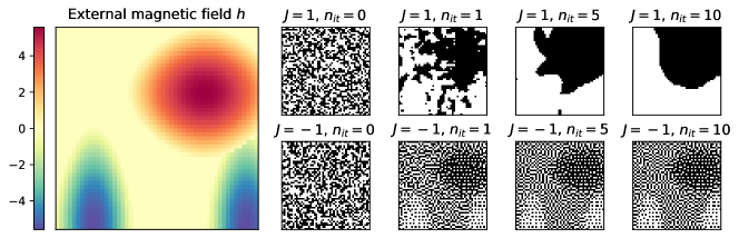
Figure 2: The external magnetic field $h$ (left) can vary spatially and influence the sampling probability relative to its strength. The sign of the coupling constant $J$ determines whether neighboring spins attract (top right) or repel each other (bottom right).

Energy-based Models.  Energy-based models are defined by an energy function $E_{\theta}\colon{\mathbb{R}}^{d}\to{\mathbb{R}}$, parameterized by $\theta$. The density defined by an energy-based model is given by the Boltzmann distribution

$$p_{\theta}(x)=Z_{\theta}^{-1}\exp(-\beta E_{\theta}(x)),$$ (1)

where $\beta>0$ is the inverse temperature and the normalization constant $Z=\int\exp(-\beta E_{\theta}(x))\mathrm{d}x$, also known as the partition function, is typically intractable.

A sample with low energy will have a higher probability than a sample with high energy. Many approaches have been proposed for training energy-based models (Song & Kingma, 2021), but most of them target the generative setting where a training dataset is given and training amounts to (approximate) maximum likelihood estimation.

Ising Model.  The Ising model corresponds to a deceptively simple energy-based model that is straightforward to express on a graph ${\mathcal{G}}=({\mathcal{V}},{\mathcal{E}})$ consisting of a tuple of a set of nodes ${\mathcal{V}}$ and a set of edges ${\mathcal{E}}\subseteq{\mathcal{V}}\times{\mathcal{V}}$ connecting the nodes. Specifically, the Ising energy is of the form

$$E(x)=-\sum_{(i,j)\in{\mathcal{E}}}J_{ij}x_{i}x_{j}-\sum_{i\in{\mathcal{V}}}h_{i}x_{i},$$ (2)

where the nodes (indices $i,j$) are associated with spins $x_{i}\in\{\pm 1\}$, the interactions $J_{ij}\in{\mathbb{R}}$ determine whether the behavior is ferromagnetic ($J>0$) or antiferromagnetic ($J<0$), and $h_{i}$ is the external magnetic field.

It follows from Equation (2) that in the absence of an external magnetic field, neighboring spins strive to be parallel in the ferromagnetic case and antiparallel in the antiferromagnetic case. An external magnetic field that can vary across nodes influences the sampling probability of the corresponding nodes. The system is disordered at high temperatures (small $\beta$) and ordered at low temperatures.

Graph Neural Networks.  A graph neural network (GNN) consists of multiple message-passing layers (Gilmer et al., 2017). Given a node feature $x_{i}^{k}$ at node $i$ and edge features $e_{ij}^{k}$ between node $i$ and its neighbors $\{j\colon j\in\mathcal{N}(i)\}$, the message passing procedure at layer $k$ is defined as

$$m_{ij}^{k} =f^{\text{m}}(x_{i}^{k},x_{j}^{k},e_{ij}^{k}),$$ (3)

$$\hat{x}_{i}^{k+1} =f^{\text{a}}_{j\in\mathcal{N}(i)}(m_{ij}^{k}),$$ (4)

$${x}_{i}^{k+1} =f^{\text{u}}(x_{i}^{k},\hat{x}_{i}^{k+1}),$$ (5)

where $f^{\text{m}}$ is the message function, deriving the message from node $j$ to node $i$, and $f^{\text{a}}_{j\in\mathcal{N}(i)}$ is a function that aggregates the messages from the neighbors of node $i$, denoted $\mathcal{N}(i)$. The aggregation function $f^{\text{a}}$ is often just a simple sum or average. Finally, $f^{\text{u}}$ is the update function that updates the features for each node. A GNN consists of message-passing layers stacked onto each other, where the node output from one layer is the input of the next layer.

To reveal the message-passing structure of the Ising model, note that we can rewrite the energy in Equation (2) as

$$E(x) =-\sum_{i\in{\mathcal{V}}}x_{i}\cdot\left(h_{i}+\sum_{j\in\mathcal{N}(i)}J_{ij}x_{j}\right)$$ (6)

$$=-\sum_{i\in{\mathcal{V}}}x_{i}h^{\text{eff}}_{i}(x),$$

where we have defined the effective magnetic field

$$h^{\text{eff}}_{i}(x)=h_{i}+\sum_{j\in\mathcal{N}(i)}J_{ij}x_{j}.$$ (7)

Equation (6) can be viewed as a message-passing step in a graph neural network, where $m_{ij}^{k}=J_{ij}x_{j}^{k}$ is the message function $f^{\text{m}}$, the aggregation $f^{\text{a}}$ function is the sum $\hat{x}_{i}^{k+1}=\sum_{j\in\mathcal{N}(i)}m_{ij}^{k}$, and the update function $f^{\text{u}}$ is ${x}_{i}^{k+1}=-x_{i}^{k}\left(h_{i}+\hat{x}_{i}^{k+1}\right)$.

Gradient Estimation in Discrete Models.  Let $p_{\theta}(x)$ be a discrete probability distribution and assume that we want to estimate the gradient of a loss defined as the expectation of a loss $\ell(x)$ over this distribution, i.e.,

$$\mathcal{L}(\theta)=\mathbb{E}_{x\sim p_{\theta}(x)}\left[\ell(x)\right].$$ (8)

Because of the discreteness, it is not possible to compute a gradient directly using backpropagation. Through a simple algebraic manipulation, we can rewrite this expression as

$$\nabla_{\theta}\mathbb{E}_{x\sim p_{\theta}(x)}\left[\ell(x)\right]=\mathbb{E}_{x\sim p_{\theta}(x)}\left[\ell(x)\nabla_{\theta}\log p_{\theta}(x)\right],$$ (9)

which is called the REINFORCE estimator (Williams, 1992). Though general, it suffers from high variance. A way to reduce this variance is to instead use the REINFORCE Leave-One-Out (RLOO) estimator (e.g., Shi et al. (2022)),

$${(\nabla_{\mathbf{\theta}}\mathcal{L})}_{\mathrm{LOO}}^{K}=\frac{1}{K}\sum_{k=1}^{K}\left(\ell(x^{(k)})-\bar{\ell}_{j}\right)\nabla_{\theta}\log p_{\theta}(x^{(k)}),$$ (10)

where $\bar{\ell}_{j}=\frac{1}{K-1}\sum_{j=1,j\neq k}^{K}\ell(x^{(j)})$.

3 Method

In graph neural network terminology, the interactions $J_{ij}$ and the external magnetic fields $h_{i}$ could be viewed as edge and node features, respectively. In particular, we use a GNN to parameterize the external magnetic field, $h_{\theta}\colon\mathcal{G}\to\mathbb{R}^{|{\mathcal{V}}|}$.

Sampling.  We use the Metropolis-Hastings algorithm to sample from the probability distribution defined by the Ising model according to Equation (1), see Algorithm 1. However, to make it computationally efficient, we parallelize it by first coloring the graph such that nodes of the same color are never neighbors.

Then, we can simultaneously perform the Metropolis-Hastings update for all nodes of the same color. For grid-structured graphs, such as images, a simple checkerboard pattern gives a perfect coloring. To extend this to general graphs, we run a greedy graph coloring heuristic (Miller et al., 1999) that produces a coloring with a limited, but not necessarily minimal, number of colors $C$.

Algorithm 1 Monte Carlo Sampling of the Ising Model

  Input: Graph $\{\mathbf{G}_{c}\}_{c=1}^{C}$ grouped by color $c$, interactions term $J$, external magnetic field $h$, number of iterations $T$.

  Output: State configuration $x\in\{\pm 1\}^{|{\mathcal{V}}|}$.

  for $i=1$ to $|{\mathcal{V}}|$ do

     $x_{i}\sim U(\{-1,1\}$) {Sample an initial state}

  end for

  for $t=1$ to $T$ do

     for $c=1$ to $C$ do

        for all nodes $x_{i}\in\mathbf{G}_{c}$ do

           $\Delta E_{i}=2x_{i}\left(J\sum_{j\in\mathcal{N}(i)}x_{j}+h_{i}\right)$

           $r\sim U([0,1])$ {Sample $r$ uniformly at random}

           if $\Delta E_{i}<0$ or $\exp(-2\beta\Delta E)>r$ then

              $x_{i}=-1\cdot x_{i}$ {Flip the spin of node $i$}

           end if

        end for

     end for

  end for

Controlling the Sampling Fraction.  For some tasks, the obvious way to minimize the loss is to either sample all nodes or none. To counteract this, we need a way to control the fraction of nodes to sample or, equivalently, to control the average magnetization $\eta$, which is defined as

$$\eta =\frac{1}{|\mathcal{V}|}\sum_{i=1}^{|\mathcal{V}|}\mathbb{E}_{x\sim p_{\theta}(x)}\left[x_{i}\right],$$ (11)

where $x\in\{\pm 1\}_{i=1}^{|{\mathcal{V}}|}$ denotes the vector containing all states and $x_{i}$ is the $i$th entry in $x$. Let $\bar{x}_{i}=\mathbb{E}_{x\sim p_{\theta}(x)}\left[x_{i}\right]$ denote the local magnetization at node $i$. Since the Markov blanket of a node is precisely its neighborhood, we can use Equation (6) to rewrite the local magnetization as

$$\bar{x}_{i} =\mathbb{E}_{j\in\mathcal{N}(i)}\left[\mathbb{E}_{i}\left[x_{i}\mid x_{j}\right]\right]$$ (12)

$$=\mathbb{E}_{j\in\mathcal{N}(i)}\left[\tanh(\beta h^{\text{eff}}_{i}(x))\right].$$ (13)

The corresponding mean-field (variational) approximation is a nonlinear system of equations in $\bar{x}$ (MacKay, 2003):

$$\bar{h}^{\text{eff}}_{i}(\bar{x}) =h_{i}+\sum_{j\in\mathcal{N}(i)}J_{ij}\bar{x}_{j},$$ (14)

$$\bar{x}_{i} =\tanh(\beta\bar{h}_{i}^{\text{eff}}).$$

Solving this yields a deterministic way of approximating the average magnetization $\eta$. However, we are primarily interested in the ordered regime, where $\beta\bar{h}^{\text{eff}}_{i}$ is large, and it approximately holds that $x_{j}=J_{ij}x_{i}$, which implies that $\bar{x}_{i}=\tanh(\beta h_{i})$ and, thus,

$$\tilde{\eta}_{\text{det}}=\frac{1}{|\mathcal{V}|}\sum_{i=1}^{|\mathcal{V}|}\tanh\left(\beta h_{i}\right).$$ (15)

This can be contrasted with the stochastic estimate we get from using a one-sample Monte Carlo estimate in Equation (13):

$$\tilde{\eta}_{\text{sto}}=\frac{1}{|\mathcal{V}|}\sum_{i=1}^{|\mathcal{V}|}\tanh\left(\beta h^{\text{eff}}_{i}(x))\right),\quad x\sim p_{\theta}(x).$$ (16)

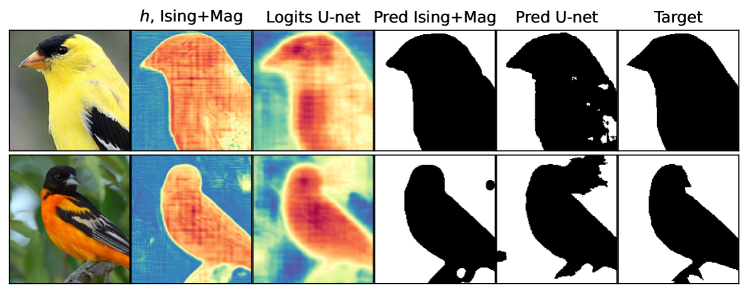
Figure 3: Comparison of a U-Net trained with a cross-entropy loss against an Ising model with a learned magnetic field. The sequence from left to right includes the original image, the magnetic field from the Ising model, the U-Net output (the logits), the Ising model prediction, the U-Net prediction, and the actual segmentation mask.

Learning.  In contrast to most other energy-based models (Song & Kingma, 2021), we do not have a training dataset we want to sample from, nor do we consider the regression setting (Gustafsson et al., 2020). Instead, we consider the unsupervised setting where the subsampled graph is used for a downstream task with an associated, possibly non-differentiable, loss.

For gradient-based training of the GNN in our Ising model, we need the gradient of the log probability. This can be decomposed as a sum of two terms:

$$\nabla_{\theta}\log p_{\theta}(x)=-\beta\nabla_{\theta}E_{\theta}(x)-\nabla_{\theta}\log Z_{\theta}.$$ (17)

We are particularly interested in training the model for a downstream task associated with a loss $\ell(x)$ defined in terms of samples $x\sim p_{\theta}(x)$ from the Ising model. The goal is then to minimize the expected loss as defined in Equation (8)

Since we are operating in a discrete setting, we use the gradient estimation technique described in Section 2. Specifically, using $K=2$ in Equation (10), the problematic $\log Z_{\theta}$ terms cancel in the RLOO estimator, and we obtain

$${(\nabla_{\mathbf{\theta}}\mathcal{L})}_{\mathrm{LOO}}^{2}= -\frac{\beta}{2}\left(\ell(x^{(1)})-\ell(x^{(2)})\right)$$ (18)

$$\quad\cdot\nabla_{\theta}\left(E_{\theta}(x^{(1)})-E_{\theta}(x^{(2)})\right).$$

To train the model, we can thus draw two independent samples $x^{(1)},x^{(2)}\sim p_{\theta}(x)$ from the Ising model and estimate the gradient using Equation (18), where $\nabla_{\theta}\left(E_{\theta}(x^{(1)})-E_{\theta}(x^{(2)})\right)$ can be computed by automatic differentiation.

To control the sampling fraction, as described in Section 1, we could either include a regularization term that depends on the stochastic sampling fraction (Equation (16)) directly in the task-specific loss $\ell$, or use a deterministic approximation based on Equation (15) to move it outside the expectation and thereby enable direct automatic differentiation. Empirically, we found the latter option to work better. Specifically, we use the training loss

$$\mathcal{L}_{\emph{tot}}(\theta) =\mathbb{E}_{x\sim p_{\theta}(x)}\left[\ell(x)\right]+(\tilde{\eta}_{\text{det}}(\theta)-\eta)^{2},$$ (19)

where the desired value of the average magnetization $\eta$ is defined as in Equation (11).

4 Applications

The proposed scheme for energy-based graph subsampling is demonstrated on three distinct applications: image segmentation, 3D shape sparsification, and sparse approximate matrix inverse determination.

4.1 Illustrative Example on Image Segmentation

While the primary goal is to learn Ising models on graphs, we initially delve into an image task due to its visual and explanatory simplicity. An image can fundamentally be seen as a simple graph, with the pixels as nodes and the neighboring pixels as neighbors (Geman & Geman, 1984). Specifically, in the ferromagnetic scenario with $J=1$, Ising models tend to group nearby pixels with the same values. Postprocessing the output of a neural network with such a probabilistic graphical model is well-known to improve the localization of object boundaries (Chen et al., 2017).

Our Approach.  Because of the grid structure, the message from the 8-connected neighbors can be implemented as a convolutional layer with kernel size three and zero padding. Specifically, we use convolutional filters of the form

$$W=\begin{bmatrix}w^{*}&w&w^{*}\\ w^{\phantom{*}}&0&w^{\phantom{*}}\\ w^{*}&w&w^{*}\end{bmatrix},$$ (20)

where $w$ and $w^{*}$ have the same sign but can have different values. This gives us the energy per pixel,

$$E_{i}=-x_{i}\left(\text{Conv}_{W}\left(x_{i}\right)+h_{\theta}(x_{i})\right).$$ (21)

Here, $h_{\theta}(x_{i})$ is the external magnetic field with the learnable parameters $\theta$. In contrast to Zheng et al. (2015), who use the mean-field approximation in Equation (14) to learn a fully connected conditional random field end-to-end, our approach applies to graph-structured energy functions and allows task-specific losses.

Since we consider binary segmentation, we use a pixel-wise misclassification loss

$$\ell(x)=\frac{1}{|{\mathcal{V}}|}\sum_{i=1}^{|{\mathcal{V}}|}|x_{i}-y_{i}|,$$ (22)

where $y_{i}\in\{-1,1\}$ is the target value.

Results.  We use the Caltech-UCSD Birds-200-2011 dataset (Wah et al., 2011) and model the magnetic field of the Ising model by a U-Net (Ronneberger et al., 2015). See Appendix B.1 for details.

Directly training the model for segmentation using a standard cross-entropy loss yields an average Dice score of 0.85 on the test set. In contrast, using a learned magnetic field in the Ising model, the average Dice score increases to 0.87 on the test set. Figure 3 compares two predictions from the two models. Notably, the output from the magnetization network of the Ising model exhibits clearer and sharper borders compared to the logits predicted by the plain segmentation model. This distinction is also evident in the predictions, where the segmentation mask predicted by the Ising model is more even and self-consistent.

4.2 3D Shape Sparsification

An object’s 3D mesh or point cloud tends to have a densely sampled surface, resulting in numerous redundant 3D points. These redundant points increase the computational workload in subsequent processing stages. Consequently, mesh and point cloud coarsening (representing the object with fewer vertices and edges) are common preprocessing steps in computer graphics (Wright et al., 2010). The main techniques for coarsening a mesh are based on preserving the spectral properties of the original mesh (Chen et al., 2022; Keros & Subr, 2022). However, these methods cannot be adapted to specific downstream tasks.

In the case of 3D point clouds, standard approaches for reducing the number of points include random subsampling and using approximation schemes with hierarchical tree structures like octrees. But these can only be adapted to the extent that prior knowledge of the geometry of the scanned object or application exists (Tenbrinck et al., 2019). While we primarily focus on mesh coarsening in the experiments, we emphasize that the same procedure can be applied to point clouds, e.g., by utilizing the relative distances between points as edge features. Importantly, we retain the positions of the original nodes that are subsampled.

Problem Formulation.  A triangular mesh $\mathcal{M}$ consists of vertices $\mathcal{V}$, edges $\mathcal{E}$ and faces $\mathcal{F}$, where the faces define which vertices belong to each triangle in the mesh. To coarsen the mesh, we remove a selection of vertices from the mesh, and the edges connected to the removed vertices are collapsed to their closed vertex. See, e.g., Figure 1.

The vertex selection can depend on any downstream task and does not have to be differentiable. In this example, we define the task as creating a coarse mesh that is as close in space to the original mesh as possible. We quantify this as the vertex-to-mesh distance between the vertices $\mathcal{V}^{1}$ in the original mesh and the surface of the coarse mesh $\mathcal{M}^{2}$,

$$d(\mathcal{V}^{1},\mathcal{M}^{2})=\sum_{x\in\mathcal{V}^{1}}\min_{y\in\mathcal{M}^{2}}||x-y||^{2}_{2}.$$ (23)

For each vertex in mesh $\mathcal{M}^{1}$, the algorithm finds the nearest point on the mesh $\mathcal{M}^{2}$ and sums the distances.

Table 1: Mean and standard deviation of the test vertex-to-mesh distance from the five-fold cross-validation of the four datasets.

dataset	Bust	Fourleg	human	chair
ISING+MAG	0.0221 (0.0042)	0.0339 (0.0034)	0.0366 (0.0031)	0.0369 (0.0046)
ISING	0.0288 (0.0055)	0.0411 (0.0034)	0.0409 (0.0033)	0.0548 (0.0045)
RANDOM	0.0343 (0.0064)	0.0498 (0.0032)	0.0498 (0.0032)	0.0592 (0.0040)

Our Approach.  We view mesh coarsening as a sampling problem, where the antiferromagnetic Ising model determines the distribution of the vertices in the coarse mesh. The antiferromagnetic Ising is a promising choice for mesh sampling because of its distinctive “every other” pattern. Unlike random sampling, which may result in concentrated points in certain areas while neglecting crucial parts of the mesh, the Ising model’s samples aim to be distributed more evenly across the entire mesh. Furthermore, the learned external magnetic field $h_{\theta}(x)$ encourages sampling in regions of particular relevance for the task at hand.

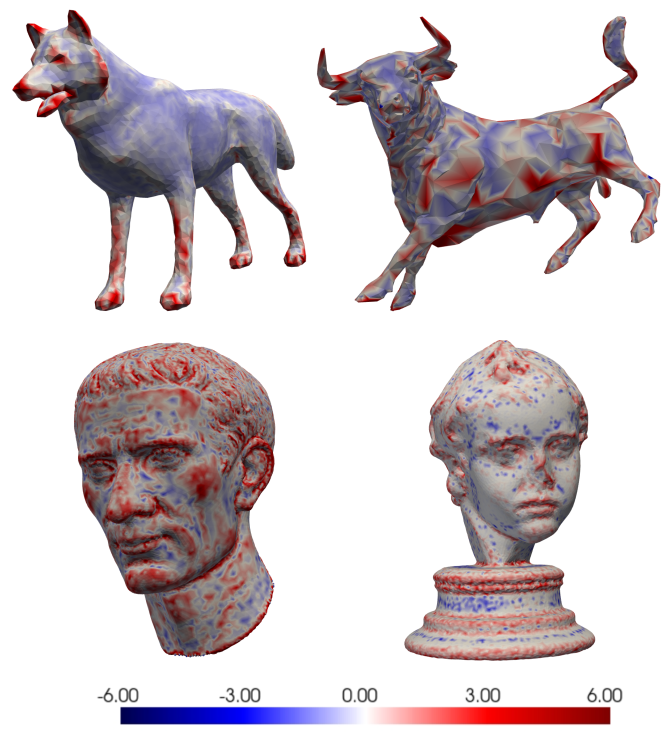
Figure 4: Four examples of learned magnetic fields from the four-leg dataset (top row) and the bust dataset (bottom row).

We represent the object’s 3D shape with a graph, with the vertices’ positions as node features and the relative distance between the nodes as edge features, $e_{ij}=x_{i}-x_{j}$. To model the magnetic field $h_{\theta}(\cdot)$, we use a three-layer Euclidean graph neural network (Geiger & Smidt, 2022) since it allows us to learn concise representations that capture crucial geometric 3D information while, at the same time, being equivariant to the rotations and translations of the mesh. We also make use of the mesh Laplacian (Reuter et al., 2009), which gives a measure of the geometry of the surfaces (see Appendix C).

From the fine mesh $\mathcal{M}^{1}$, we generate a coarse mesh $\mathcal{M}^{2}$ by sampling vertices using the Ising model. From the selected vertices, we then regenerate the mesh by collapsing the unused vertices to their closest neighbors. To learn the external magnetic field $h_{\theta}(\cdot)$, we use the RLOO gradient estimator defined in Equation (18). The loss function is defined in Equation (19), where $\ell(\cdot)$ is the distance defined in Equation (23).

Results.  We use the mesh segmentation dataset (Chen et al., 2009), and learn separate models for each of the classes bust, four-leg, human, and chair. Each class contains 20 different meshes. We evaluate the model using five-fold cross-validation, where we train on 80% of the dataset and test on the remaining 20%. The meshes contain between 4712 and 27439 vertices. More details can be found in Appendix C. We train the models until convergence on the training dataset, using $\eta=0$ in Equation (19), which means we aim to reduce the number of vertices in the mesh by half.

The results from our experiments are summarized in Table 1. Notably, Ising sampling without an external magnetic field leads to a reduction in the vertex-to-mesh distance between the original vertices and the coarse mesh compared to random sampling. This is further improved by including a learned magnetic field. Figure 4 provides a visual representation of the predicted magnetic field for four meshes in the test dataset. By visual inspection, we can see that the magnetic field is high in areas where we have sharp corners and generally more intricate geometry. To compensate for the high magnetic field in certain areas, our regularization term forces it to be low in other areas that are not as important for the task, i.e., the vertex-to-mesh distance. Figure 1 provides a closer look at the samples from the Ising model with a learned magnetic field. Note the higher concentration of samples in high curvature regions such as the dog’s ear and nose.

4.3 Sparse Approximate Matrix Inverses

In many scientific and technical domains, solving large linear systems on the form $Az=b$, where $A\in{\mathbb{R}}^{n\times n}$ is a sparse system matrix, remains a frequently encountered computational challenge. With increasing problem sizes, direct solution methods are replaced by iterative methods such as the Krylov subspace methods. If the setting is ill-conditioned, however, these methods require preconditioning of the original system (e.g., Häusner et al. (2023)). Sparse approximate inverses are often suitable preconditioners in large-scale applications.

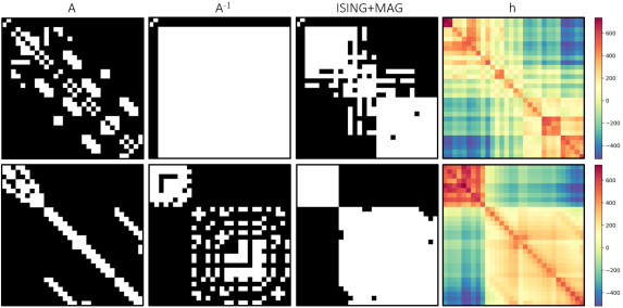
Figure 5: Rows show two matrices from the test dataset (Setting 3). Each sparsity pattern shows nonzero elements (white) in the corresponding matrix. From the left: (a) sparsity pattern of $A$, (b) sparsity pattern of true inverse $A^{-1}$, (c) sparsity pattern of the approximate inverse using the $50\%$ of all matrix elements predicted by our model, (d) predicted magnetic field for the given matrix $A$.

Problem Formulation.  We are interested in finding a sparse approximate inverse $M\approx A^{-1}\in{\mathbb{R}}^{n\times n}$ constituting the right preconditioner for the sparse linear system $Az=b$. Given a sparsity pattern $s\in\mathcal{S}$ of the matrix $M$, where $s$ is a collection of $m$ a priori determined indices corresponding to the non-zero matrix entries in $M$, and $\mathcal{S}$ is the space containing all possible sparsity patterns, we want to solve the following optimization problem for the values $s^{\prime}\in{\mathbb{R}}^{m}$ of the non-zero entries in $M$

$$\min_{s^{\prime}\in\mathbb{R}^{m}}{\lVert AM^{\prime}(s)-I\rVert}_{\mathrm{F}}.$$ (24)

Here, $\|\cdot\|_{\mathrm{F}}$ denotes the Frobenius norm and $I$ is the $n\times n$ identity matrix. With this notation, $M^{\prime}(s)$ denotes the approximate inverse with sparsity pattern $s$ and nonzeros $s^{\prime}$.

While elegant, this approach does require an a priori assumption on the sparsity pattern $s$, which directly affects the quality of the preconditioner that can be obtained. Various modifications to the described sparse approximate inverse approach (SAI) exist, aiming to refine the sparsity pattern iteratively (Grote & Huckle, 1997).

Our Approach.  We use the proposed approach for graph subsampling with learned Ising models to find promising sparsity patterns for sparse approximate inverse determination. To do this, we take inspiration from the graph representation of symmetric sparse linear systems (Moore et al., 2023), in which a symmetric matrix $A$ is viewed as the adjacency matrix of a weighted undirected graph and, hence, the matrix elements correspond to edge features in the undirected graph. Since the Ising model is defined over nodes, we move from the current graph representation to its line graph (e.g., Sjölund & Bånkestad (2022)). With a zero magnetic field, the Ising model encodes an a priori assumption of the nonzeros being equally distributed over the rows and columns when applied to the line graph. Here, we simulate the Ising model on the line graph using a magnetic field $h$ parameterized by a GNN. A sample $x$ from the resulting distribution then corresponds to the proposed sparsity pattern $s$ of the predicted sparse approximate inverse $M$ of the input matrix $A$.

The learning objective is to minimize the total expected loss with respect to the trainable parameters $\theta$, while reducing the number of elements in an a priori sparsity pattern (possibly including all elements) by $50\%$. To do this, we use the training loss given in Equation (19), with

$$l(x)={\lVert AM(s^{\theta}(x))-I\rVert}_{\mathrm{F}},$$ (25)

and $\eta=0$. Here, $M(s^{\theta}(x))$ denotes the specific approximate inverse obtained by solving Equation (24) using the sparsity pattern obtained from a sample of the learned Ising model given its current parameter state. To model the external magnetic field, we use a graph convolutional network (Chen et al., 2020). For training, we use the RLOO gradient estimator according to Equation (18), and let $A$ and $A^{2}$ enter as edge features. Contrary to conventional approaches, our method is flexible in terms of a priori sparsity patterns. Any a priori sparsity pattern can be induced by the graph representation, and thus, no such assumptions are theoretically necessary. See Appendix D.1 and B.3 for further details on the model specifics, training process, and implementation.

Datasets.  We test our approach on two datasets consisting of real, sparse, and symmetric $30\times 30$ matrices. Dataset 1 consists of $1600$ synthetic, binary sparse matrices. Dataset 2 consists of 1800 sparse $30\times 30$ submatrices constructed from the SuiteSparse Matrix Collection (Davis & Hu., 2011), and the matrices in this dataset thus resemble sparse matrices from real-world applications. The mean sparsity of the matrices in Dataset 1 is $83\%$, and the corresponding sparsity level for Dataset 2 is $89\%$. Independent on the dataset, $60\%$ of the data is used for training, and $20\%$ is used for validation and testing, respectively. Further details on the datasets and preprocessing can be found in Appendix D.2.

Results.  We train three separate models, each in a different setting. In Setting 1, we use Dataset 1 and add $A$ and $A^{2}$ as edge features. In practice, this means that the a priori sparsity pattern of the approximate inverse is effectively the sparsity pattern of $A^{2}$, and the model is optimized to select $50\%$ of these elements for the sparsity pattern of the predicted sparse approximate inverse $M$. In Setting 2, $A$ and $A^{2}$ remain edge features, but the model is optimized to select $50\%$ of all elements for the sparsity pattern of $M$, see Appendix D.1 for implementation details. Setting 3 is identical to Setting 2, but uses Dataset 2 in place of Dataset 1.

Table 2 shows the results in terms of the mean loss, calculated according to Equation (25), over the test dataset in each setting, evaluated using a single sample from the learned Ising model for each test matrix. We compare the performance of our model (ISING+MAG) to three competing approaches: a) an Ising model with a small constant magnetic field tuned to obtain the same sampling fraction as the one recorded on the corresponding test set (Ising), b) uniform random sampling from the allowed sparsity pattern in each setting with the corresponding sampling fraction (Random), and c) the quality of the sparse approximate inverse obtained using only the sparsity pattern of input matrix $A$ (Only A), which is a common a priori assumption on the sparsity pattern when determining sparse approximate matrix inverses. In all cases, we observe a significant improvement in the mean loss compared to the baselines.

Table 2: Mean and standard deviation of the loss on the test set for each model and setting.

Model	Setting 1	Setting 2	Setting 3
ISING+MAG	3.28 (0.12)	2.06 (0.26)	1.15 (1.24)
ISING	3.86 (0.12)	3.69 (0.23)	3.78 (0.42)
RANDOM	4.04 (0.16)	3.86 (0.18)	3.86 (0.30)
Only A	4.12 (0.08)	4.12 (0.08)	2.00 (1.89)

Results for two samples from the test dataset in Setting 3 are visualized in Figure 5, showing in particular how the learned magnetic field has adapted to allow for sampling of a sparsity pattern capturing important regions when the true inverses have inherently different structures. The results are discussed in detail in Appendix D.1.

5 Related Work

Statistical Physics.  The Ising model was one of the first tractable analytical models of magnetic systems that exhibit phase transitions. Interestingly, the closer the parameter is to its critical value, the less the details of the system matter. This observation, referred to as universality in statistical physics, has motivated the generalization of the Ising model to broader classes of systems. For instance, the standard Potts model is a direct generalization of the Ising model to multiple classes (Wu, 1982). By contrast, the Ising model with continuous states $x_{i}\in[-1,1]$ is known as a spin glass system (Nishimori, 2001).

Models from statistical physics have, for a long time, been used to inspire and understand neural networks (Carleo et al., 2019). Notably, spin glasses are generally known as Hopfield networks in the machine learning community (MacKay, 2003). Again, these have continuous states $x_{i}\in[-1,1]$, yet the update rule for a Hopfield network remains the same as for the mean-field approximation of the Ising model. Over the past few years, there has been renewed interest in Hopfield networks as an unsupervised model of associative memory (Krotov & Hopfield, 2016; Demircigil et al., 2017; Ramsauer et al., 2020).

Probabilistic Graphical Models.  The Ising model, or spin glasses more generally, gave rise to the concept of a Markov random field, where a probabilistic graphical model (Koller & Friedman, 2009) is used to encode dependencies between random variables. In our model, we output the external magnetic field as an intermediate variable that we then condition on to define an Ising model. It is, therefore, appropriately described as a conditional random field (Lafferty et al., 2001). Conditional random fields are widely used for structured prediction tasks, for instance, in natural language processing (Lample et al., 2016) and computer vision (Zheng et al., 2015; Chen et al., 2017).

Graph Sparsification and Coarsening.  The goal of graph sparsification and coarsening operations is to generate a smaller graph that preserves the global structure of a large graph. A unifying framework that captures both of these operations is considered by Bravo-Hermsdorff & Gunderson (2019). In contrast to our approach, theirs is not learned; rather, they present an algorithm for reducing a graph while preserving the Laplacian pseudoinverse.

Safro et al. (2015); Loukas & Vandergheynst (2018); Loukas (2019); Jin et al. (2020) also propose algorithms for graph coarsening. Their approach is to preserve spectral properties. In contrast to those approaches, but building on top of them, Cai et al. (2021) follows an approach based on neural networks for graph coarsening. Fahrbach et al. (2020) compute a graph coarsening based on Schur complements with the goal of obtaining embeddings of relevant nodes. Deng et al. (2020) pursue a similar goal. A coarsening approach based on optimal transport is done by Ma & Chen (2021). The coarsening of graphs for the scalability of GNNs is considered by Huang et al. (2021) and Jin et al. (2022b, a) perform dataset condensation for graph data for the same scalability reasons. The goal is that GNNs perform similarly on the condensed data but are faster to train. Finally, Chen et al. (2022) provides an overview of successful coarsening techniques for scientific computing.

As for graph sparsification, Spielman & Teng (2011) do spectral sparsification, Yu et al. (2022) use an information-theoretic formulation for sparsification, and Batson et al. (2013) provide an overview on the topic of sparsification. Ushijima-Mwesigwa et al. (2017) perform graph partitioning using quantum annealing by minimizing an Ising objective.

6 Discussion and Conclusion

We presented a novel approach for graph subsampling by learning the external magnetic field in the Ising model and sampling from the resulting distribution. Moreover, we demonstrated that our approach exhibits promising potential in a wide range of applications, with no restriction on the differentiability of the loss function in a specific application. We did this using the REINFORCE Leave-One-Out gradient estimator and a carefully selected regularization structure that allows us to control the sampling fraction. Our method was demonstrated on three distinct applications. In image segmentation, we showed that our approach produced clear segmentation masks with sharp borders. In mesh coarsening, we demonstrated that the learned magnetic field promotes sampling in high curvature regions while retaining the characteristic “every other” pattern. Finally, we showed that our approach can be used to learn promising sparsity patterns for sparse approximate matrix inverse determination via Frobenius norm minimization.

Limitations and Future Work.  In the current applications, the computations are relatively fast (see Table 5 in Appendix C), but this may change in large-scale applications, where the sampling, including the graph coloring, can become a bottleneck. This is something we would like to address in future work.

Another limitation is that the Ising model only allows binary states, whereas some applications, e.g., image classification, would require multiple classes. We believe it would be possible to extend our approach to such cases by instead using the Potts model or the even more general random cluster model (Fortuin & Kasteleyn, 1972).

Appendix A Ising sampling

To illustrate the convergence rate of the Ising model, we plot the energy against the number of Monte Carlo iterations in Figure 6. These simulations are done on the 20 meshes in the Bust dataset in Section 4.2. We plot the mean plus the standard dedication of the model energy at each iteration. We observe that the ferromagnetic ($J=1$) or antiferromagnetic ($J=-1$) Ising model converges fast, even though the antiferromagnetic one converges faster in just a handful of iterations.

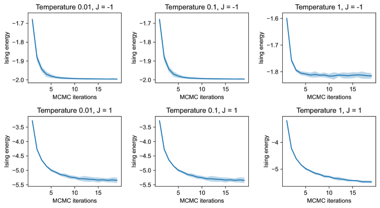
Figure 6: The mean and standard deviations of the Ising model energy against the number of Monte Carlo iterations for the ($J=1$) or antiferromagnetic ($J=-1$) Ising model. The simulation is also done for three different temperatures: 0.01, 0.1, and 1.

Appendix B Implementation details

Here, we go through the details of our models and training procedures for the applications in Section 4. We used one GPU, NVIDIA GeForce RTX 3090, for all the experiments, and we performed all the experiments using less than 10 GPU hours.

B.1 U-Net

We trained a U-Net of the bird segmentation task in Section 4.1 using a U-Net with three down-sampling blocks, one middle layer, and three up-sampling blocks. The implementation is inspired by https://github.com/yassouali/pytorch-segmentation/tree/master. The dimensions of the blocks/layers are presented in Table 3.

Table 3: Dimensions of the U-Net blocks.

Layer	input dim	output dim
Input layer	3	16
Encoder 1	16	32
Encoder 2	32	64
Encoder 3	64	128
Mid layer	128	128
Decoder 1	128	64
Decoder 2	64	32
Decoder 3	32	16
Output layer	16	1

We train the model using the Adam optimizer (Kingma & Ba, 2015), a batch size of 32, and a learning range of 1e-4. The dataset contains 6537 segmented images. We split the dataset in a train/val/test split using the ratios 0.8/01/0.1. We train the model for 300 epochs and test the model with the lowest evaluation error. Here, we use a temperature of one and $J=1$ for the Ising model.

B.2 Equivariant graph network

The equivariant graph neural network in Section 4.2 is constructed using the e3nn library (Geiger & Smidt, 2022). As the node input, we derive the mesh Laplacian according to

$$\mathbf{C}_{ij}=\begin{cases}\frac{\cot\alpha_{ij}~{}+\cot\beta_{ij}}{2}&\text{if }i,j\text{ is an edge}\\ -\sum_{j\in N(i)}{C_{ij}}&\text{if }i\text{ is in the diagonal}\\ 0&\text{otherwise},\end{cases}$$ (26)

where and $\alpha_{ij}$ and $\beta_{ij}$ denote the two angles opposite of edge $(i,j)$ (Sorkine, 2005). We get a measure of the curvature of the node using

$$z_{i}^{0}=||\sum_{i=\mathcal{N}(i)}\mathbf{C}_{ij}(\hat{r}_{i}-\hat{r}_{j})||^{2}_{2},$$ (27)

where $\hat{r}_{i}$ is the position of node i. We use $z_{i}^{0}$ as the model node input. As edge attributes, we use the spherical harmonics expansion of the relative distance between node $i$ and its neighbors $j$, $Y\left((\hat{r}_{i}-\hat{r}_{j})/||\hat{r}_{i}-\hat{r}_{j}||)\right)$ and the node-to-node distance $d_{ij}=||\hat{r}_{i}-\hat{r}_{j}||$. We construct an equivariant convolution by first deriving the message from the neighborhood as

$$\hat{z}^{k+1}_{i}=\frac{1}{n_{d}}\sum_{j\in\mathcal{N}(i)}z_{j}^{k}\otimes_{f_{W}(d_{i}j)}Y\left(\frac{\hat{r}_{i}-\hat{r}_{j}}{||\hat{r}_{i}-\hat{r}_{j}||}\right),$$ (28)

where $n_{d}$ is the mean number of neighboring nodes of the graph. For a triangular mesh, the degree is commonly six. The formula $\otimes_{f_{W}(d_{i}j)}$ defines the tensor product with distant dependent weights $f_{W}(d_{i}j)$; this is a two-layer neural network with learnable weights $w$ that derives the weights of the tensor product. The node features are then updated according to

$${z}^{k+1}_{i}=z^{k}_{i}+\alpha\cdot\hat{z}^{k+1}_{i},$$ (29)

where $\alpha$ is a learnable residual parameter dependent on $z^{k}_{i}$. We took inspiration for the model from the e3nn homepage, see https://github.com/e3nn/e3nn/blob/main/e3nn/nn/models/v2106/points_convolution.py.

We construct a two-layer equivariant network where the layer irreducible representations are [0e, 16x0e + 16x1o, 16x0e]. This means that the input (0e) consists of a vector of 16 scalars, and the hidden layers consist of vectors with 16 scalars (16x0e) together with 16 vectors (16x1o) of odd parity. This, in turn, maps to the output vector of 16 scalars (16x0e). We subtract the representation with the mean of all nodes in the graph and finally map this representation to a single scalar output. Here, we use a temperature of one and $J=-1$ for the Ising model.

For optimization, we employ the Adam optimizer (Kingma & Ba, 2015) with a learning rate of 0.001 and a batch size of one. We train the model until convergence on the training set but with a maximum number of 50 epochs. We did not use a validation set as there were no indications of overfitting.

B.3 Graph convolutional neural network

Here, we use the simple and deep graph convolutional networks from Chen et al. (2020) where we set the strength of the initial residual connection $\alpha$ to $0.1$ and $\theta$, the hyperparameter to compute the strength of the identity to $0.5$. The network contains 4 layers, and each has a hidden dimension of 64. We utilize weight sharing across these layers. The dimension of the output of the final convolutional layer is 64. This output is subtracted with the mean of the node values before a final linear layer reduces the size to one.

For optimization, we employ the Adam optimizer (Kingma & Ba, 2015) with a learning rate of 0.01. We train the model until convergence on the training set but with a maximum number of 300 epochs, as there were no indications of overfitting. Here, we use a temperature of one and $J=-0.4$ for the Ising model.

Appendix C Mesh coarsening details

This section contains extra information on the mesh coarsening experiments in Section 4.2. The details of the mesh dataset are compiled in Table 4. The time it takes to sample points and construct the course mesh for the different methods is presented in Table 5. Additional predicted magnetic fields from the test split from the four different datasets are found in Figures 7, 8, 9, and 10. An illustration of the course meshes after sampling is presented in Figure 11.

Table 4: Details of the meshes in the dataset used in Section 4.2.

dataset	Bust	Fourleg	human	chair
Number of vertices	25662 (1230)	9778 (3671)	8036 (4149)	10154 (999)
Number of faces	51321 (2460)	19553 (7342)	16070 (8302)	20313 (2002)

Table 5: Mean sampling and coarsening time for the three different methods.

	Bust		Fourleg		Human		CHair
Model	Samp	Coars	Samp	Coars	Samp	Coars	Samp	Coars
Ising + mag	0.19 (0.064)	1.30 (0.53)	0.13 (0.050)	0.37 (0.16)	0.13 (0.052)	0.45 (0.16)	0.33(0.50)	0.46(0.077)
Ising	0.13 (0.048)	1.08 (0.41)	0.10 (0.028)	0.34 (0.15)	0.10 (0.30)	0.42 (0.17)	0.10(0.034)	0.39(0.071)
Random	2.4e-4 (4e-4)	2.07 (0.83)	1e-4 (2e-4)	0.52 (0.24)	9.23e-5 (3.1e-4)	0.68 (0.31)	1.75e-4(2.86e-4)	0.61 (0.14)

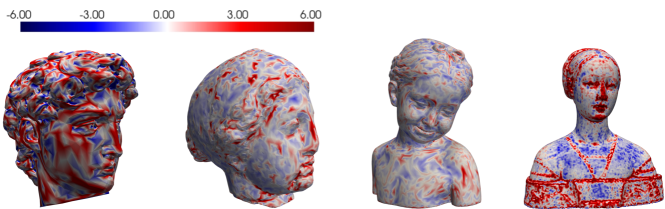
Figure 7: Examples of the magnetic field from the bust dataset (test set).

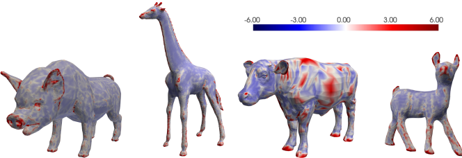
Figure 8: Examples of the magnetic field from the four-leg dataset (test set).

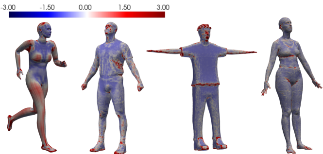
Figure 9: Examples of the magnetic field from the human dataset (test set).

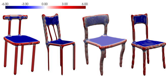
Figure 10: Examples of the magnetic field from the chair dataset (test set).

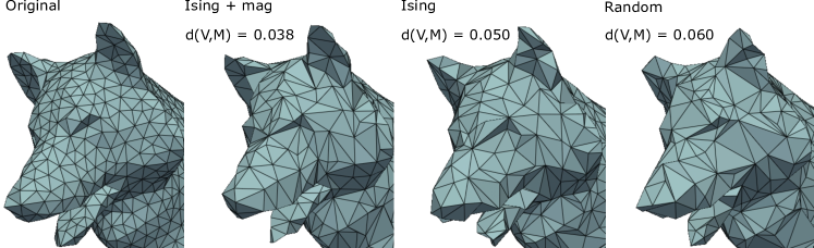
Figure 11: The coarsened mesh using random subsampling, Ising subsampling, and learned Ising subsampling of the nodes. The point-to-mesh distance is reduced from 0.06 to 0.038 when going from the random subsampling to the learned Ising graph. The time it takes to sample and create the course mesh are: random, 1.37 sec, Ising 0.67 sec, and Ising + mag 1.31 sec. The reason the random sampling takes longer time is due to a more complicated course mesh creation.

Appendix D Sparse Approximate Matrix Inverses

D.1 Results and implementation details

With our initial model architecture, the graph representation induces an a priori assumption on the sparsity pattern of the predicted sparse approximate inverse in which we aim to select $50\%$ of the elements in the sparsity pattern of $A+A^{2}$. Our approach is, however, not limited to the choice of an a priori sparsity pattern. Implementation-wise, we lift this constraint by adding an extra edge feature consisting of an all-ones $n\times n$ matrix in the graph representation of the input matrix, allowing for a selection of $50\%$ of all matrix elements in the sparse approximation of the inverse. As the a priori sparsity pattern is already incorporated into the graph representation of the input matrix, this renders our method flexible in terms of choice of a priori sparsity pattern, which in our case should be denser than the desired sparsity level. This flexibility is expected to be especially important for computational efficiency in use cases involving large matrix dimensions.

Given the current state of the trainable parameters, two samples from the Ising model are required during training to obtain the gradient estimate. Evaluation is carried out using a single sample. In both cases, the sample $x$ from the Ising model produced after $T$ MCMC iterations is passed to the final layer, which solves the the $n$ optimization problems,

$$s^{*}_{k}=\operatorname*{arg\,min}_{s^{\prime}_{k}\in\mathcal{R}^{m_{k}}}{\lVert AM_{k}(s_{k})-I_{k}\rVert}^{2}_{2},$$ (30)

computing the values $s^{*}_{k}\in{\mathbb{R}}^{m}$ of the non-zero entries of each column $M_{k}$ of $M$. Thus, the final output is the predicted sparse approximate inverse $M$. Empirically, $T=3$ is found to be sufficient.

Independent on which dataset is used, $60\%$ of the samples are used for training, and the remaining $40\%$ are divided equally between a validation set and a test set. We use the magnetic field-dependent regularization described in Section 1 to optimize for a sampling fraction of $50\%$ of the a priori sparsity pattern. In all settings, the sampling fraction converges to an average value close to $50\%$ with the proposed regularization scheme. The mean recorded sampling fraction on the test dataset in Setting 1 and Setting 2 is $52.4\%$ and $50.9\%$, respectively. The corresponding sampling fraction in Setting 3 is $49.8\%$. The baseline methods are tuned to allow for the same sampling fraction during evaluation.

Results for two samples from the test dataset in Setting 3 are visualized in Figure 5. The first sample (top) shows the predicted sparsity pattern when the true inverse is dense. For this sample, the recorded loss is $2.61$ (ISING+MAG) compared to $3.57$ (Ising), $4.18$ (Random) and $4.12$ (Only A). As discussed in Figure 2, the magnitude of the local magnetic field influences the sampling probability in that region, which can be seen by comparing the output magnetic field to the obtained sparsity pattern for both samples. A zero magnetic field in the Ising model can be interpreted as a prior on the sparsity pattern in which $50\%$ of the elements in each row and column of the matrix are selected, resulting in an inverse approximation in which the nonzero elements are evenly distributed across the given matrix. For the second sample (bottom), the sparsity optimized for is lower than the sparsity of the true inverse. We choose to display this sample as the results clearly illustrate that the learned magnetic field indeed results in an Ising model from which the sampled sparsity pattern successfully avoids the most unimportant regions in the true inverse for the particular input matrix. For this sample, the recorded loss is $1.02$ (ISING+MAG) compared to $3.75$ (Ising), $3.76$ (Random) and $4.06$ (Only A).

D.2 Datasets

Dataset 1.  This is a synthetic dataset containing 1600 binary matrices. Each matrix is real, symmetric, and of dimensionality $30\times 30$. The matrices in the dataset are automatically generated based on the principle that the probability of a nonzero element increases towards the diagonal, with $100\%$ probability of nonzero diagonal elements. The upper right and lower left corners have a very low probability of being nonzero, and in between these elements and the diagonal, the probability of a nonzero element varies according to a nonlinear function. The mean sparsity is $83\%$ zero-elements in the generated dataset. The maximum sparsity allowed in the data-generating process is $96\%$, and the determinant of each matrix is bounded between $0.001$ and $50$. Figure 12 shows sparsity patterns of four matrices in the final dataset.

The dataset is available upon request and will be released together with the code used for preprocessing and generation.

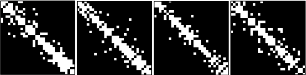
Figure 12: Example of samples from Dataset 1. Nonzero elements are represented in white.

Dataset 2.  This is a synthetic dataset containing 1800 submatrices of size $30\times 30$ constructed from the SuiteSparse Matrix Collection (Davis & Hu., 2011). Since the original matrices in the dataset are often denser closer to the diagonal, the submatrices are constructed by iterating a window of size $30\times 30$ along the diagonals, such that no submatrix overlaps another submatrix. To ensure that each submatrix is symmetric, only the upper triangular part of the matrix is used to create each matrix. Each submatrix is scaled such that the absolute value of the maximum element is one, and submatrices with all values below $10^{-6}$ are removed from the dataset. The mean sparsity in the final dataset is $89\%$. The maximum sparsity allowed in the data-generating process is $96\%$, and the determinant of each matrix is bounded between $0.001$ and $50$. Figure 13 shows sparsity patterns of four matrices in the final dataset.

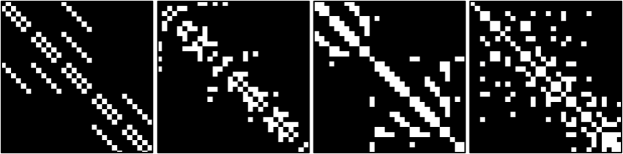
Figure 13: Example of sparsity patterns of samples from Dataset 2. Nonzero elements are represented in white.

The original dataset is under the CC-BY 4.0 License. Our modified dataset is available upon request and will be released with the code used for preprocessing and generation.

References

- Batson et al. (2013) Batson, J., Spielman, D. A., Srivastava, N., and Teng, S.-H. Spectral sparsification of graphs: theory and algorithms. Communications of the ACM, 56(8):87–94, 2013.
- Bravo-Hermsdorff & Gunderson (2019) Bravo-Hermsdorff, G. and Gunderson, L. A unifying framework for spectrum-preserving graph sparsification and coarsening. In Advances in Neural Information Processing Systems, volume 32, 2019.
- Cai et al. (2021) Cai, C., Wang, D., and Wang, Y. Graph coarsening with neural networks. In International Conference on Learning Representations, 2021.
- Carleo et al. (2019) Carleo, G., Cirac, I., Cranmer, K., Daudet, L., Schuld, M., Tishby, N., Vogt-Maranto, L., and Zdeborová, L. Machine learning and the physical sciences. Reviews of Modern Physics, 91(4):045002, 2019.
- Chen et al. (2022) Chen, J., Saad, Y., and Zhang, Z. Graph coarsening: from scientific computing to machine learning. SeMA Journal, pp. 1–37, 2022.
- Chen et al. (2017) Chen, L.-C., Papandreou, G., Kokkinos, I., Murphy, K., and Yuille, A. L. DeepLab: Semantic image segmentation with deep convolutional nets, atrous convolution, and fully connected CRFs. IEEE Transactions on Pattern Analysis and Machine Intelligence, 40(4):834–848, 2017.
- Chen et al. (2020) Chen, M., Wei, Z., Huang, Z., Ding, B., and Li, Y. Simple and deep graph convolutional networks. In International Conference on Machine Learning, pp. 1725–1735. PMLR, 2020.
- Chen et al. (2009) Chen, X., Golovinskiy, A., and Funkhouser, T. A benchmark for 3d mesh segmentation. ACM Transactions on Graphics (TOG), 28(3):1–12, 2009.
- Cipra (1987) Cipra, B. A. An introduction to the Ising model. The American Mathematical Monthly, 94(10):937–959, 1987.
- Davis & Hu. (2011) Davis, T. A. and Hu., Y. The university of florida sparse matrix collection. ACM Transactions on Mathematical Software, 38(1):1–25, 2011.
- Demircigil et al. (2017) Demircigil, M., Heusel, J., Löwe, M., Upgang, S., and Vermet, F. On a model of associative memory with huge storage capacity. Journal of Statistical Physics, 168:288–299, 2017.
- Deng et al. (2020) Deng, C., Zhao, Z., Wang, Y., Zhang, Z., and Feng, Z. Graphzoom: A multi-level spectral approach for accurate and scalable graph embedding. In International Conference on Learning Representations, 2020.
- Duhamel & Vetterli (1990) Duhamel, P. and Vetterli, M. Fast Fourier transforms: a tutorial review and a state of the art. Signal Processing, 19(4):259–299, 1990.
- Fahrbach et al. (2020) Fahrbach, M., Goranci, G., Peng, R., Sachdeva, S., and Wang, C. Faster graph embeddings via coarsening. In International Conference on Machine Learning, pp. 2953–2963. PMLR, 2020.
- Fortuin & Kasteleyn (1972) Fortuin, C. M. and Kasteleyn, P. W. On the random-cluster model: I. introduction and relation to other models. Physica, 57(4):536–564, 1972.
- Geiger & Smidt (2022) Geiger, M. and Smidt, T. e3nn: Euclidean neural networks. arXiv preprint arXiv:2207.09453, 2022.
- Geman & Geman (1984) Geman, S. and Geman, D. Stochastic relaxation, Gibbs distributions, and the Bayesian restoration of images. IEEE Transactions on Pattern Analysis and Machine Intelligence, 6:721–741, 1984.
- Gilmer et al. (2017) Gilmer, J., Schoenholz, S. S., Riley, P. F., Vinyals, O., and Dahl, G. E. Neural message passing for quantum chemistry. In International Conference on Machine Learning, pp. 1263–1272. PMLR, 2017.
- Grote & Huckle (1997) Grote, M. J. and Huckle, T. Parallel preconditioning with sparse approximate inverses. SIAM Journal on Scientific Computing, 18(3):838–853, 1997.
- Gustafsson et al. (2020) Gustafsson, F. K., Danelljan, M., Timofte, R., and Schön, T. B. How to train your energy-based model for regression. In Proceedings of the British Machine Vision Conference (BMVC), September 2020.
- Hackbusch (2013) Hackbusch, W. Multi-grid methods and applications, volume 4. Springer Science & Business Media, 2013.
- Häusner et al. (2023) Häusner, P., Öktem, O., and Sjölund, J. Neural incomplete factorization: learning preconditioners for the conjugate gradient method. arXiv preprint arXiv:2305.16368, 2023.
- Huang et al. (2021) Huang, Z., Zhang, S., Xi, C., Liu, T., and Zhou, M. Scaling up graph neural networks via graph coarsening. In Proceedings of the 27th ACM SIGKDD Conference on Knowledge Discovery & Data Mining, pp. 675–684, 2021.
- Jin et al. (2022a) Jin, W., Tang, X., Jiang, H., Li, Z., Zhang, D., Tang, J., and Yin, B. Condensing graphs via one-step gradient matching. In Proceedings of the 28th ACM SIGKDD Conference on Knowledge Discovery and Data Mining, pp. 720–730, 2022a.
- Jin et al. (2022b) Jin, W., Zhao, L., Zhang, S., Liu, Y., Tang, J., and Shah, N. Graph condensation for graph neural networks. In International Conference on Learning Representations, 2022b.
- Jin et al. (2020) Jin, Y., Loukas, A., and JaJa, J. Graph coarsening with preserved spectral properties. In International Conference on Artificial Intelligence and Statistics, pp. 4452–4462. PMLR, 2020.
- Keros & Subr (2022) Keros, A. D. and Subr, K. Generalized spectral coarsening. arXiv preprint arXiv:2207.01146, 2022.
- Kingma & Ba (2015) Kingma, D. and Ba, J. Adam: A method for stochastic optimization. In International Conference on Learning Representations, 2015.
- Koller & Friedman (2009) Koller, D. and Friedman, N. Probabilistic graphical models: principles and techniques. MIT Press, 2009.
- Krotov & Hopfield (2016) Krotov, D. and Hopfield, J. J. Dense associative memory for pattern recognition. In Advances in Neural Information Processing Systems, volume 29, 2016.
- Lafferty et al. (2001) Lafferty, J. D., McCallum, A., and Pereira, F. C. Conditional random fields: Probabilistic models for segmenting and labeling sequence data. In Proceedings of the International Conference on Machine Learning, pp. 282–289, 2001.
- Lample et al. (2016) Lample, G., Ballesteros, M., Subramanian, S., Kawakami, K., and Dyer, C. Neural architectures for named entity recognition. In Proceedings of the 2016 Conference of the North American Chapter of the Association for Computational Linguistics: Human Language Technologies, pp. 260–270, 2016.
- Lindeberg (2013) Lindeberg, T. Scale-space theory in computer vision, volume 256. Springer Science & Business Media, 2013.
- Loukas (2019) Loukas, A. Graph reduction with spectral and cut guarantees. Journal of Machine Learning Research, 20(116):1–42, 2019.
- Loukas & Vandergheynst (2018) Loukas, A. and Vandergheynst, P. Spectrally approximating large graphs with smaller graphs. In International Conference on Machine Learning, pp. 3237–3246. PMLR, 2018.
- Ma & Chen (2021) Ma, T. and Chen, J. Unsupervised learning of graph hierarchical abstractions with differentiable coarsening and optimal transport. In Proceedings of the AAAI Conference on Artificial Intelligence, pp. 8856–8864, 2021.
- MacKay (2003) MacKay, D. J. Information theory, inference and learning algorithms. Cambridge University Press, 2003.
- Mallat (1999) Mallat, S. A wavelet tour of signal processing. Elsevier, 1999.
- Miller et al. (1999) Miller, G. L., Talmor, D., and Teng, S.-H. Optimal coarsening of unstructured meshes. Journal of Algorithms, 31(1):29–65, 1999.
- Moore et al. (2023) Moore, N. S., Cyr, E. C., Ohm, P., Siefert, C. M., and Tuminaro, R. S. Graph neural networks and applied linear algebra. arXiv preprint arXiv:2310.14084, 2023.
- Nishimori (2001) Nishimori, H. Statistical physics of spin glasses and information processing: an introduction. Clarendon Press, 2001.
- Pumain (2006) Pumain, D. (ed.). Hierarchy in Natural and Social Sciences, volume 3 of Methodos Series. Springer Dordrecht, 2006.
- Ramsauer et al. (2020) Ramsauer, H., Schäfl, B., Lehner, J., Seidl, P., Widrich, M., Gruber, L., Holzleitner, M., Adler, T., Kreil, D., Kopp, M. K., et al. Hopfield networks is all you need. In International Conference on Learning Representations, 2020.
- Reuter et al. (2009) Reuter, M., Biasotti, S., Giorgi, D., Patanè, G., and Spagnuolo, M. Discrete Laplace–Beltrami operators for shape analysis and segmentation. Computers & Graphics, 33(3):381–390, 2009.
- Ronneberger et al. (2015) Ronneberger, O., Fischer, P., and Brox, T. U-net: Convolutional networks for biomedical image segmentation. In Medical Image Computing and Computer-Assisted Intervention – MICCAI 2015, pp. 234–241. Springer, 2015.
- Safro et al. (2015) Safro, I., Sanders, P., and Schulz, C. Advanced coarsening schemes for graph partitioning. Journal of Experimental Algorithmics, 19:1–24, 2015.
- Shi et al. (2022) Shi, J., Zhou, Y., Hwang, J., Titsias, M., and Mackey, L. Gradient estimation with discrete stein operators. In Advances in Neural Information Processing Systems, volume 35, pp. 25829–25841, 2022.
- Shuman et al. (2015) Shuman, D. I., Faraji, M. J., and Vandergheynst, P. A multiscale pyramid transform for graph signals. IEEE Transactions on Signal Processing, 64(8):2119–2134, 2015.
- Sjölund & Bånkestad (2022) Sjölund, J. and Bånkestad, M. Graph-based neural acceleration for nonnegative matrix factorization. arXiv preprint arXiv:2202.00264, 2022.
- Song & Kingma (2021) Song, Y. and Kingma, D. P. How to train your energy-based models. arXiv preprint arXiv:2101.03288, 2021.
- Sorkine (2005) Sorkine, O. Laplacian mesh processing. Eurographics (State of the Art Reports), 4(4), 2005.
- Spielman & Teng (2011) Spielman, D. A. and Teng, S.-H. Spectral sparsification of graphs. SIAM Journal on Computing, 40(4):981–1025, 2011.
- Tenbrinck et al. (2019) Tenbrinck, D., Gaede, F., and Burger, M. Variational graph methods for efficient point cloud sparsification. arXiv preprint arXiv:1903.02858, 2019.
- Ushijima-Mwesigwa et al. (2017) Ushijima-Mwesigwa, H., Negre, C. F., and Mniszewski, S. M. Graph partitioning using quantum annealing on the d-wave system. In Proceedings of the Second International Workshop on Post Moores Era Supercomputing, pp. 22–29, 2017.
- Wah et al. (2011) Wah, C., Branson, S., Welinder, P., Perona, P., and Belongie, S. Mesh segmentations. Technical Report CNS-TR-2011-001, California Institute of Technology, 2011.
- Williams (1992) Williams, R. J. Simple statistical gradient-following algorithms for connectionist reinforcement learning. Machine Learning, 8:229–256, 1992.
- Wright et al. (2010) Wright, J., Ma, Y., Mairal, J., Sapiro, G., Huang, T. S., and Yan, S. Sparse representation for computer vision and pattern recognition. Proceedings of the IEEE, 98(6):1031–1044, 2010.
- Wu (1982) Wu, F.-Y. The Potts model. Reviews of Modern Physics, 54(1):235, 1982.
- Yu et al. (2022) Yu, S., Alesiani, F., Yin, W., Jenssen, R., and Principe, J. C. Principle of relevant information for graph sparsification. In Uncertainty in Artificial Intelligence, pp. 2331–2341. PMLR, 2022.
- Zheng et al. (2015) Zheng, S., Jayasumana, S., Romera-Paredes, B., Vineet, V., Su, Z., Du, D., Huang, C., and Torr, P. H. Conditional random fields as recurrent neural networks. In Proceedings of the IEEE International Conference on Computer Vision, pp. 1529–1537, 2015.