Ozone Anomalies in Dry Intrusions Associated with Atmospheric Rivers
Abstract
As a result of their important role in weather and the global hydrological cycle, understanding atmospheric rivers’ (ARs) connection to synoptic-scale climate patterns and atmospheric dynamics has become increasingly important. In addition to case studies of two extreme AR events, we produce a December climatology of the three-dimensional structure of water vapor and (ozone) distributions associated with ARs in the northeastern Pacific from 2004-2014 using MERRA-2 reanalysis products. Results show that positive anomalies reside in dry intrusions of stratospheric air due to stratosphere-to-troposphere transport (STT) behind the intense water vapor transport of the AR. In composites, we find increased excesses of concentration, as well as in the total flux within the dry intrusions, with increased AR strength. We find that STT flux associated with ARs over the NE Pacific accounts for up to 13% of total Northern Hemisphere STT flux in December, and extrapolation indicates that AR-associated dry intrusions may account for as much as 32% of total NH STT flux. This study quantifies STT of in connection with ARs for the first time and improves estimates of tropospheric ozone concentration due to STT in the identification of this correlation. In light of predictions that ARs will become more intense and/or frequent with climate change, quantifying AR-related STT flux is especially valuable for future radiative forcing calculations.
JGR: Atmospheres
Center for Astrophysics Harvard & Smithsonian, Radio & Geoastronomy Division Center for Astrophysics Harvard & Smithsonian, Atomic and Molecular Physics Division NASA Goddard Space Flight Center, Atmospheric Chemistry and Dynamics Laboratory GESTAR II, Morgan State University
60 Garden St., Cambridge, MA 02138, USA Greenbelt, MD, USA Baltimore, MD, USA
Kirsten Hallkirsten.hall@cfa.harvard.edu
Case studies and December climatology using MERRA-2 reveal positive tropospheric ozone anomalies within dry intrusions associated with ARs.
Average excess ozone concentrations are 10-13 ppbv at 400 hPa, and are even greater for increasing intensity of ARs.
STT of ozone associated with ARs in the NE Pacific may account for (13 2)% of the total December Northern Hemisphere STT ozone flux.
Plain Language Summary
Long filaments of rapidly moving water vapor in the atmosphere, known as atmospheric rivers (ARs), play a vital role in the Earth’s water cycle. Because of this, research continues to expand into ARs’ relationship with large-scale climate patterns. In this paper, we use data from the Modern Era Retrospective analysis for Research Applications to examine several extreme ARs that made landfall on the U.S. West Coast and their relationship to the transport of ozone from the stratosphere to the troposphere. We then combine eleven years of December AR and ozone data in order to study the average trend of ozone transport in connection with ARs. We quantify the AR-related ozone transport for the first time, and we find ARs with more intense water vapor transport result in the transport of higher concentrations of ozone. Quantifying ozone transport into the troposphere in connection with ARs is important as ARs may become more intense and/or more frequent with climate change, and ozone in the troposphere has consequences for the greenhouse effect.
1 Introduction
Atmospheric rivers (ARs) are streams of water vapor in the lower troposphere that are typically defined as being at least 2000 km in length and 1000 km in width. They are often associated with warm conveyor belts of ascending moist air travelling along and ahead of the cold fronts of extratropical cyclones (ECs) [Dacre \BOthers. (\APACyear2015), Eiras-Barca \BOthers. (\APACyear2018), Guo \BOthers. (\APACyear2020)]; though about 20% occur not in connection with an EC, and neither the intensity nor the precise location or duration of the AR can be determined from the cyclone [Zhang \BOthers. (\APACyear2019)]. They are the primary mode by which water vapor is transported from the tropics towards the poles [Newell \BOthers. (\APACyear1992), Newell \BBA Zhu (\APACyear1994), Zhu \BBA Newell (\APACyear1998)]. They occur all over the globe, and there is a high concentration of recent studies focused on expanding the global characterization and analysis of ARs [<]e.g.,¿Shie18, Coll20, Coll22.
The intensity of ARs, as defined by the integrated vapor transport (IVT), is variable, and strong AR events can have catastrophic consequences, such as flooding and mudslides. Throughout this analysis, we investigate composites of IVT and ozone profiles connected to ARs with a range of intensities with IVT250 kg m-1 s-1 and a range of duration from less than 24 hours to more than 72 hours. \citeARalp19 devises a categorization scheme for ARs as Cat 1-5, and we will use this as a reference in discussing some events. Climate model projections using Phase 5 of the Coupled Model Intercomparison Project (CMIP5) indicate that their intensity (IVT strength) will increase in the warming future by up to 25%, and their frequency will increase by anywhere from 30% to 300% globally, depending on the definitions of the number of AR days in different detection algorithms [Gao \BOthers. (\APACyear2015), Espinoza \BOthers. (\APACyear2018)]. As a result of their important role in weather and the global hydrological cycle, understanding ARs’ connection to planetary- and synoptic-scale climate patterns and atmospheric dynamics has become increasingly important.
Of particular interest is the impact of upper-tropospheric dynamics on ARs and vice versa. For example, several studies link ARs and extreme precipitation events directly to Rossby wave breaking (RWB) [<]e.g.,¿Payn14, Ryoo15, Payn16, Hu17,Moor19. In an assessment of the connection between intense moisture transport and RWB, \citeAdeVr21 finds that the depth of the wave breaking and intensity of the integrated vapor transport are both directly correlated with the severity of extreme precipitation. That is, through the analysis of the depth of folding of PV contours, they find that the deeper the breaking, the more intense the water vapor transport.
With a clear connection between moisture transport and RWB, it follows to investigate a connection to the transport dynamics from the stratosphere to the troposphere. Stratosphere-troposphere transport (STT) or exchange (STE) of air masses on a planetary scale is a consequence of Rossby waves propagating into the stratosphere and mesosphere. This phenomenon leads to both the rising of air from the troposphere to the stratosphere in the tropics, and a descent at mid- and high- latitudes [Holton \BOthers. (\APACyear1995), Nath \BOthers. (\APACyear2016)]. PV anomalies or streamers exist as a result of dry intrusions of ozone-rich stratospheric air that lag behind the transport of moist air from the equatorial lower troposphere poleward and into the upper troposphere [Waugh (\APACyear2005)]. These PV intrusions as a result of STE increase the tropospheric ozone () concentrations [Nath \BOthers. (\APACyear2016)].
In addition to the planetary-scale continuous downward flow of air masses, in the extratropics, STE also occurs as an episodic phenomenon in association with synoptic-scale processes that perturb the tropopause. For example, STE in connection with ECs has been well-documented [<]e.g.,¿Dani68, John81, Holt95, Wern02, Reut15. Dry intrusions, or dry airstreams [Browning (\APACyear1997)], of stratospheric ozone-rich air are a defining characteristic in the cold sector of synoptic-scale low pressure systems, and they are also described by relatively high potential vorticity (PV) in a folding or lowering of the tropopause. \citeAJaeg17 produces the climatology of positive anomalies due to STE in dry intrusions associated with ECs, finding these events contribute up to 42% of the total STE flux. We aim to provide in this work a similar assessment of STE of in PV intrusions linked to December AR events in the northeast (NE) Pacific.
Understanding the total stratospheric contribution to tropospheric concentrations has been a significant area of research for several decades [Monks (\APACyear2000), Stohl \BOthers. (\APACyear2003), Lefohn \BOthers. (\APACyear2011), Škerlak \BOthers. (\APACyear2014), Abalos \BOthers. (\APACyear2020)]. Tropospheric is a greenhouse gas and key contributor to climate change [Lacis \BOthers. (\APACyear1990), Worden \BOthers. (\APACyear2011)], and it is a pollutant at the surface, harmful to humans and plants. impacts the oxidation capacity of the atmosphere affecting the chemical pathway of formation and loss of many species with crucial consequences for radiative forcing. Due to STE, there remain large discrepancies amongst chemical transport models’ predictions of tropospheric , which impedes a reasonable understanding of the total concentration due to photochemistry [Young \BOthers. (\APACyear2013), Young \BOthers. (\APACyear2018), Morgenstern \BOthers. (\APACyear2018), Griffiths \BOthers. (\APACyear2021)]. Disentangling the contributions to tropospheric by STE from the production of due to precursor emissions is vital for understanding air pollution and future warming due to greenhouse gases.
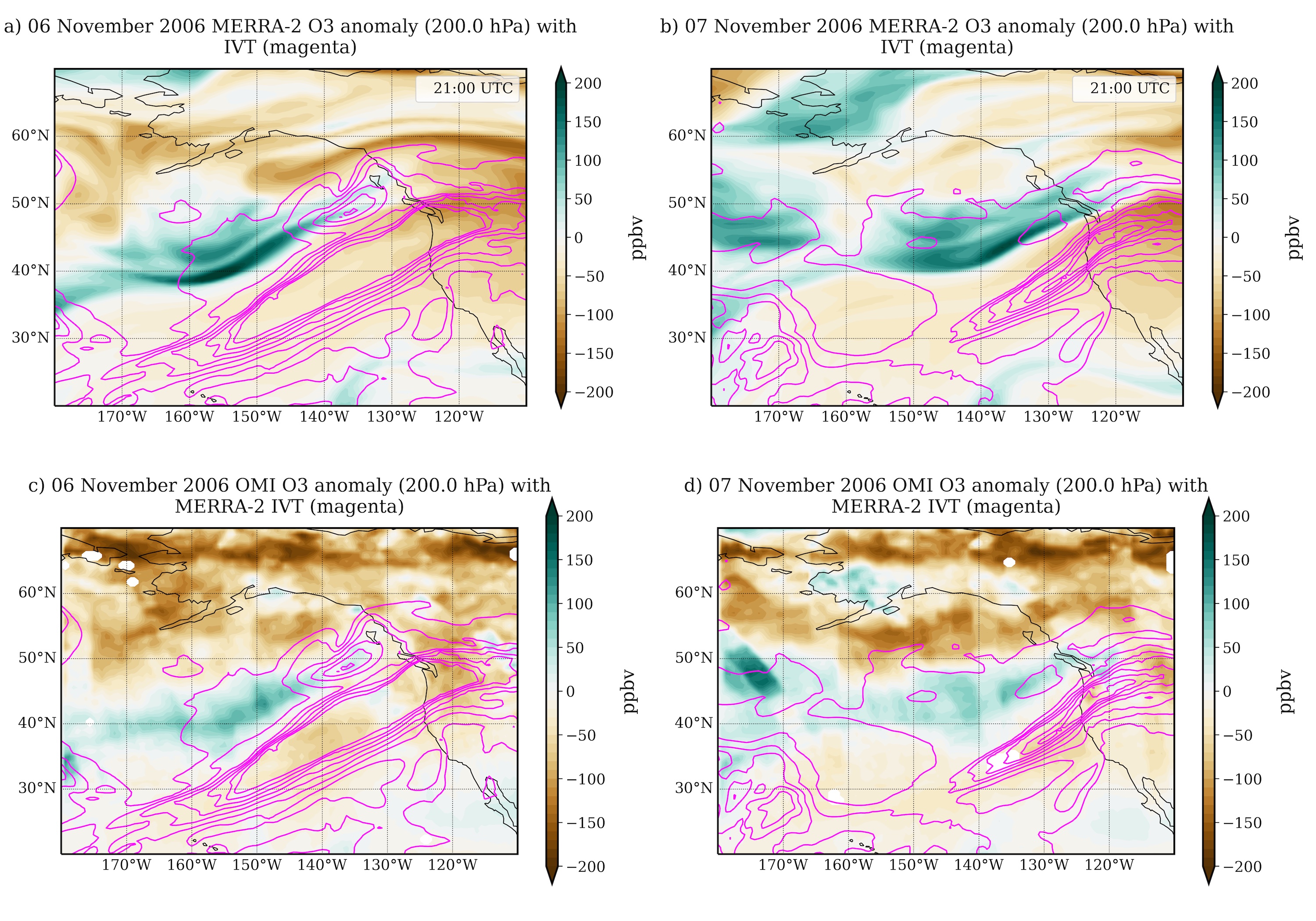
In the application study of water vapor retrieval from the Ozone Monitoring Instrument [<]OMI,¿Leve06, \citeAWang19 discovered anomalous concentrations at the level of the tropopause trailing an exceptional (Cat 5) atmospheric river event on 06-07 November 2006 (Figure 1, bottom row). This AR occurred over the northeast Pacific and brought detrimental flooding to the Pacific Northwest upon landfall. The details of this event are described in \citeANeim08a. The anomaly appears to the northwest of the AR, mirroring the curvature of the AR as a long filament of excess relative to the November decadal climatology, both computed from the OMI mixing ratio data interpolated to 200 hPa. OMI data suggest paired anomalies in the upper tropospheric and total column water vapor in this AR event. This discovery inspired a detailed analysis of the time evolution of the three-dimensional structure of the and water vapor distributions associated with representative AR events using the MERRA-2 reanalysis product. While approximately 82% of ARs in the North Pacific are formed in connection with ECs [Zhang \BOthers. (\APACyear2019)], they are distinct phenomena of varying size, evolution, and duration relative to their cyclone counterparts, thus we aim to quantify the STE in relation to ARs and their physical properties.
In this paper, we uncover the relationship between ARs and associated anomalies in tropospheric concentrations as a result of related stratosphere-troposphere exchange (STE). The scope of this work focuses broadly on ARs over the NE Pacific and western North America; first, we give a detailed view of several ARs, then we present composites of December ARs over an eleven year period. We describe the data in Section 2, our analysis methods, including tracking ARs over their lifetime, and our composite analysis in Section 3. Section 4 details our assessment of anomalous associated with two exceptional (Cat 5) [Ralph \BOthers. (\APACyear2019)] AR events in November 2006 and December 2010, as well as a complete assessment of all ARs in December 2010. We extend this analysis to all of December 2004-2014 with a statistical summary and composite results, including average IVT, anomaly, and vertical cross sections in Section5. In this section, we also compute the average STT flux and divide our sample into two bins of AR IVT to assess the correlation between excess and AR intensity. We summarize and conclude in Section 6.
2 Data
2.1 Ozone Monitoring Instrument (OMI)
We validate our use of MERRA-2 profiles by comparing MERRA-2 mixing ratios and anomalies to those retrieved from OMI onboard the Aura spacecraft. OMI is an imaging spectrometer that covers visible-UV wavelengths from 350-500 nm, and has been making daily global measurements since October 2004 at nominal nadir spatial resolutions of 13×48 km and 13x24 km for spectral windows UV1 and UV2, respectively, from a polar orbit with 13:30 Equator crossing local time. The 10-year OMI Ozone Profile (PROFOZ) product used in this study was validated with ozonesondes [G. Huang \BOthers. (\APACyear2017)] and Microwave Limb Sounder [G. Huang \BOthers. (\APACyear2018)] measurements. Compared to ozonesondes observations, OMI profiles were found to have mean biases less than 6% in the midlatitudes down to an average of 550 hPa [G. Huang \BOthers. (\APACyear2017)]. In comparison to MLS, the profiles are found to have negative global mean biases between 3-9% below approximately 100 hPa [G. Huang \BOthers. (\APACyear2018)]. These biases are due to a combination of OMI retrievals and MLS having a positive bias at these altitudes compared to other measurements [Froidevaux \BOthers. (\APACyear2008)]. The standard deviations are approximately 27% and 20% at these latitudes and pressure levels in comparison with ozonesondes and MLS, respectively [G. Huang \BOthers. (\APACyear2017), G. Huang \BOthers. (\APACyear2018)].
Specifically, we use daily profiles, first generated with a regridding of 0.5∘ x 0.5∘ resolution to improve the SNR and speed up production from \citeALiu10 for 06 and 07 November 2006. We refer the reader to \citeALiu10, \citeAHuan17, and \citeAHuan18 for the full details of the profiles retrievals and validations. \citeAWang19 used these data regridded at 1∘ x 1∘ in an application demonstrating the retrieval of Total Column Water Vapor (TCWV) from OMI for the AR event on these dates and discovered the high mixing ratio concentrations parallel to the northwest of the excess TCWV from the AR. We then regrid our 0.5∘ latitude by 0.5∘ longitude OMI data to the MERRA-2 resolution of 0.5∘ latitude by 0.625∘ longitude using the publicly available python bilinear method regridding algorithm xESMF.Regridder [Zhuang \BOthers. (\APACyear2023)] for our comparison in Section 4.1.
2.2 Modern-Era Retrospective analysis for Research and Applications, Version 2 (MERRA-2)
The atmospheric data products used in this analysis are taken or calculated from the Modern-Era Retrospective analysis for Research and Applications, Version 2 [<]MERRA-2,¿Gela17 reanalysis, which covers the period of January 1980 through to within a couple weeks of real-time, at a horizontal resolution of 0.5 × 0.625° latitude-by-longitude. MERRA-2 assimilates meteorological and observations using the updated Goddard Earth Observing System Model (GEOS) model and data assimilation system [Molod \BOthers. (\APACyear2015), Gelaro \BOthers. (\APACyear2017)]. In particular, we select data sets with an instantaneous 3-hourly temporal resolution with 42 pressure levels from 1000 hPa to 0.01 hPa, as well as the monthly mean instantaneous products, and use meteorological and chemical products for winds (u,v), temperature, specific humidity, Ertel’s PV, relative humidity, sea level pressure, and mixing ratios [Global Modeling and Assimilation Office (GMAO) (\APACyear2015\APACexlab\BCnt1), Global Modeling and Assimilation Office (GMAO) (\APACyear2015\APACexlab\BCnt2)]. The GEOS model system for MERRA-2 uses the Goddard 2D chemistry and transport model to derive linearly interpolated daily values for both the stratosphere and the troposphere [Nielsen \BOthers. (\APACyear2017), Knowland \BOthers. (\APACyear2022)].
Prior to 2004, MERRA-2 assimilated profiles from several NOAA Solar Backscatter Ultraviolet (SBUV/2) instruments. After 2004, and for years relevant to this work, MERRA-2 improves upon the ozone assimilation with total column ozone from OMI, as well as version 2.2 ozone retrieval from Aura’s Microwave Limb Sounder [<]MLS,¿Wate06 for which the recommended vertical range is 215 hPa to 0.02 hPa as described in [Wargan \BOthers. (\APACyear2017)]. Ozone mixing ratios from MERRA-2 in the lower stratosphere agree with the Stratospheric Aerosol and Gas Experiment II measurements to within 5 in the extratropics, and once OMI and MLS data were assimilated, the bias drops to 2 [Wargan \BOthers. (\APACyear2017)]. \citeAWarg17 reports similar 5 bias in the extratropics (30-60∘N) in comparison to ozonesondes observations of stratospheric ozone. In the upper troposphere within the SBUV period, the bias is within 10 of the ozonesondes [Wargan \BOthers. (\APACyear2015)]. In the Aura period after 2004, the low sensitivity of OMI columns to mixing ratios for 500 hPa along with the simple chemistry in the assimilation system [Wargan \BOthers. (\APACyear2017)] cause the MERRA-2 tropospheric to be biased low by 13.6 on average in comparison to ozonesondes between 30-60∘N. Given the agreement in the lower stratosphere, tropospheric measurements of mixing ratio inside of dry, stratospheric intrusion events are expected to be reliable except for the consideration that the background in the troposphere is biased due to the simple chemistry transport, which is inconsequential for this study. \citeAKnow17 shows that the vertical structure of in stratospheric intrusions over the western United States is well captured by MERRA-2, and that MERRA-2 has high enough horizontal resolution to capture filaments [<]as also demonstrated in¿Ott16. This analysis primarily identifies excess anomalous in dry intrusions in the upper troposphere. Any assessment below roughly 500 hPa is trustworthy as it is within the stratospheric intrusion as similarly found in \citeAKnow17 and \citeAJaeg17.
2.3 AR Identification Catalog
To identify ARs, we use the binary tag files from the Atmospheric River Tracking Method Intercomparison Project [<]ARTMIP,¿Shie18 MERRA-2 Tier 1 catalogues [Rutz \BOthers. (\APACyear2019)]. ARTMIP is an international collaboration to quantify uncertainties in AR science based on the details of detection algorithms. The Tier 1 catalogues are a set of AR catalogues all created using MERRA-2 data, but with differing detection criteria and implemented on varying geographical regions, global and otherwise. Our primary criteria in this study for an AR identification catalog is that they cover the NE Pacific Ocean, classify ARs with a broad range of intensities – as indicated by the integrated water vapor transport (IVT), and specifically IVT 250 kg m s-1 – and track them for the duration of their lifetime. Moreover, using a catalog that identifies ARs globally is useful for future analyses of in dry intrusions associated with ARs globally. There are many methods for identifying ARs, and based on our criteria, we opted to primarily use the ARTMIP binary tag catalogue generated using the algorithm from \citeARutz14.
The \citeARutz14 detection algorithm uses selection criteria that enforce the AR length to be at least 2000 km and the minimum absolute integrated water vapor transport (IVT) from surface to 100 hPa to be greater than or equal to 250 kg m-1 s-1. The catalog is global, and \citeARutz14 provides an analysis of the climatology of the characteristics of ARs over the Western United States. The algorithm used to detect ARs in \citeARutz14 was originally run on the Interim European Centre for Medium-Range Weather Forecasts (ECMWF) Re-Analysis (ERA-Interim; \citeADee11) data. We acquired the catalog from the NCAR Climate Data Gateway as a part of Tier 1 of the ARTMIP project, in which the \citeARutz14 algorithm was run on the MERRA-2 3-hourly data to generate binary tags – 0s for no AR in that grid cell and time step and 1s for AR present at that location and time.
In this work, we examine any relationship between the amplitude of anomaly and flux and AR strength. The \citeARutz14 algorithm is conservative in its categorization of ARs, allowing us to sample the full range of AR IVTs (down to peak IVT of 250 kg m-1 s-1). As a check on the dependence of our results on our catalog, we ran our algorithm using several other ARTMIP Tier 1 participating developer AR identification catalogs for December 2010 and obtained the same results for each one. The additional catalogs we tested used algorithms from: \citeAKash21 ClimateNet deep learning algorithm, and \citeAReid20 Reid250 with absolute IVT250 kg m-1 s-1. We intentionally tested other algorithms for which the IVT values are allowed to be at least as low as 250 kg m-1 s-1. The ClimateNet deep learning algorithm imposes no minimum IVT threshold, and the Reid250 algorithm imposes an additional length-width requirement. There was no dependence of our results on the choice of AR binary tag catalog, likely because we only track one AR at a time as identified by the maximum IVT in the region, and so long as the selection criteria includes ARs with IVT250 kg m-1 s-1, then we are likely to identify at least the same ARs over our geographical area. Other criteria could have imposed differing lifespans of ARs, but in spite of any differences we find out results unchanged. If instead we were to choose an algorithm with a more strict IVT threshold, we would miss AR time steps that drop below that, but that would go against our intended purpose of comparing a wide range of possible AR intensities, so we did not test this.
3 Analysis Methods
Here we detail the various components of our analysis. The general algorithm progresses as follows: use MERRA-2 data to compute IVT in the NE Pacific, apply a mask of binary tags that identify ARs at each time step, track individual ARs through their lifetime, and simultaneously identify nearby anomalies that are a result of dry intrusions. We track the evolution of the ARs using the binary tags and peak IVT values at each time step, as well as the vertical structure of the associated dry intrusion using PV. The peak IVT value, direction of the AR (), peak anomalous concentration, and locations of the peaks are all stored for further analysis. We also describe our calculation of flux inside the dry intrusions and the computation of composite IVT and O3 anomalies.
3.1 Atmospheric river tracking
We built an algorithm to track ARs through their lifetime. We make maps of vertically integrated water vapor transport (IVT, kg m-1 s-1) computed as,
| (1) |
where q is the specific humidity, and u and v are the zonal and meridional layer-averaged wind components, respectively, all of which are taken from MERRA-2 3-hourly datasets. The integral runs over each layer’s pressure increment, dp, and g is the acceleration due to gravity. Using the binary tag catalog from \citeARutz14 as a mask on the IVT maps to identify the locations of ARs, we find the peak amplitude of the IVT in the NE Pacific Ocean, from 180∘W to 110∘W and 25∘N to 60∘N, at each three hour time step beginning on 01 December at 00:00 for each year between 2004-2014. We also run this algorithm on November 2006 data. The decision to choose the maximum IVT means we are choosing the most intense AR in the field at the initial time step, but as the algorithm is designed to follow ARs until they dissipate, we still sample a wide range of AR intensities. We also keep track of the AR direction of travel defined according to \citeAPan19 as,
| (2) |
where and are the zonal and meridional IVT components defined by,
| (3) |
and
| (4) |
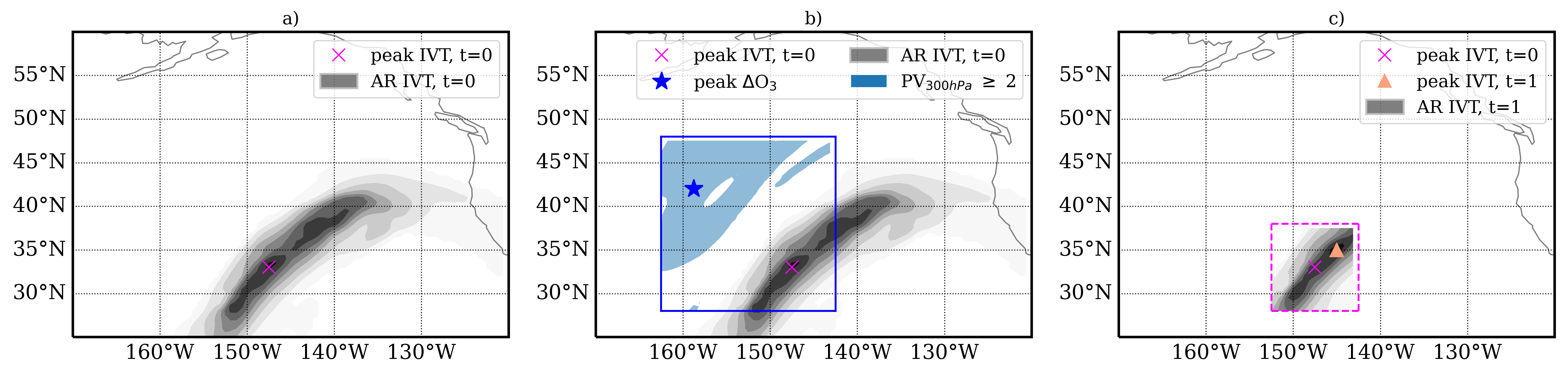
Once the algorithm identifies a new AR, it follows the AR through its remaining lifespan by searching within a 10∘ latitude by 10∘ longitude box centered on the initial peak IVT location for the peak IVT at the next time step. This is exemplified in steps one and three of Figure 2 (left and right panels). When the peak IVT within this smaller field drops to zero, the search box returns to the original area encompassing the NE Pacific to search for the next AR event. This enables us to determine at each 3-hourly time step the peak IVT of a single AR event throughout the majority of its lifetime. The algorithm only tracks one AR at a time; therefore, it may miss the initial stages of an AR’s development. Additionally, if the peak IVT increases by more than 125 kg m-1 s-1 compared to the previous time step, the algorithm checks for the peak IVT in the entire NE Pacific area because such an increase in IVT may indicate that a different AR has entered the search field. If the location of that peak is more than 1000 km from the previous peak location or more than 450 kg m-1 s-1 greater than the previous time step’s IVT, then that new peak IVT is determined to be associated with a new AR.
3.2 STT identification and characterization
enhancements in the UT/LS often result from the transport of dry, ozone-rich stratospheric air down toward and into the troposphere behind the cold front of the EC and/or AR. The enhancement can be associated with a complete folding or simply a lowering of the dynamic tropopause. While some intrusions might be associated with both an EC and an AR if the AR is coincident with the EC, we are making a distinct measurement of intrusions associated with ARs. ARs occur in coincidence with ECs approximately 82% of the time [Zhang \BOthers. (\APACyear2019)], but even in these instances, the anomaly may be distinct from that associated with the EC and/or may evolve with the AR and persist for a longer duration of time [Mundhenk \BOthers. (\APACyear2016), Zhang \BOthers. (\APACyear2019)]. For comparison, \citeAJaeg17 provides a complete analysis of the in dry intrusions to the southwest of ECs in the Northern Hemisphere (NH). Similarly, \citeAKnow15 quantify tropospheric enhancement in the area encompassing the most intense (95th percentile) spring ECs over the North Pacific and North Atlantic.
In order to better understand the relationship between anomalous and ARs, we track the excess in proximity to several AR case studies and in composites. We compute anomalies by subtracting the relevant monthly climatology over the years 2004-2014. We track the tropopause lowering or folding using the PV provided by MERRA-2. We use the dynamical tropopause definition of whichever isosurface is lower: PV2 PVU (1 PVU = 10-6 K m2 kg-1 s-1), or 380K [Hoskins \BOthers. (\APACyear1985), Holton \BOthers. (\APACyear1995)]. After identifying the AR and its peak IVT, our algorithm identifies potential tropopause lowering using PV contours, PV2 at 300 hPa within 15∘ N, 15∘ W, 5∘ S, and 5∘ E of the location of the peak IVT (Figure 2, middle). We then locate the peak anomalous concentration within the dry intrusion at the 200 hPa and 400 hPa pressure levels. Maximum anomalies at these pressure levels are also required to lie outside the AR as determined by the binary mask as an additional means of identifying the tropopause fold or lowering. Figure 2 demonstrates the process of identifying the AR, its peak IVT, and maximum anomalous concentration at some time t=0, then shows the box that is search for the peak IVT at the next time step, t=1. The algorithm repeats steps two and three with peak IVT at the new time step replacing the previous value and location until the AR dissipates or a new, more intense AR enters the smaller search box.
In order to track and characterize the depth of the dry intrusions and the STT of , we use the vertical pressure cross section over a geodesic line defined according to the peak IVT and the maximum anomaly at 400 hPa. Along this cross-section, we identify the dynamic tropopause, which in this case is always the PV=2 contour. By tracking this contour, we follow the tropopause folding or lowering and record its maximum depth (highest pressure level reached). We are careful to ensure the contour is connected to the stratosphere and is not part of a cutoff according to \citeASker14. This is exemplified in the case study analyses in Section 4 and the results are further explored in Section 5.
A further quantity of interest is the flux due to STT. Following a similar method to \citeAJaeg17, we quantify the total in the dry intrusion between the local 2 PVU dynamical tropopause and the level 75 hPa below the climatological dynamical tropopause, which we compute to be 275 hPa using the MERRA-2 PV data for the eastern part of the North Pacific in December 2004-2014 between 25∘ N to 60∘ N and 180∘ W to 110∘ W. This computation puts the upper bound on the dry intrusion at 350 hPa, and any individual dry intrusion for which the tropopause lowering does not reach below 350 hPa is not considered deep enough for any irreversible mixing of to have occurred during the STT [Jaeglé \BOthers. (\APACyear2017)]. We first calculate the vertical integral of from the maximum depth of the dry intrusion (PV2 contour) up to 350 hPa to obtain the flux (kg m-2). For the average daily flux, we track the number of days over which we calculate each individual intrusion flux and compute the mean over that number of days. We also calculate the total average flux (Tg day-1) in this manner, first as the vertical integral, then as the two dimensional integral of the positive column integrated over latitude and longitude for each intrusion, and then average over the total number of days.
3.3 Generating Composites
To quantify the relative position and maximum of the average magnitude of the positive anomalies near the AR events, statistically, we generate peak IVT-centric composites using the catalogued positions of the peak IVT for all AR time steps in December between 2004 and 2014. Because the location of the anomalies associated with each AR is dependent upon the AR direction of travel, we lessen the averaging out of anomalous peaks and troughs by dividing all of the AR time steps into seven bins according to the direction of the peak IVT (). We bin according to the direction in each tracked time step rather than individual AR events because ARs can change direction during their lifetime, enough that the relative locations of the dry intrusions are affected. For each time step in a bin, we define a 20∘ latitude x 20∘ longitude area centered on the peak IVTs and compute the mean IVT over that area for each bin. Over the same area, we compute the mean anomaly for each bin and the 200, 300, and 400 hPa atmospheric pressure levels. We also compute the vertical cross-section of the composites in the same manner as for individual events, and determine the relative location of the maximum average anomaly in these directionally divided composites. Although averaging over a large range in can dilute some of the synoptic scale information, the number of bins was chosen primarily such that we can further divide those into bins of peak IVT and each bin would still contain adequate numbers to perform a statistical assessment.
We further examine the relationship between the composite maximum anomalous and peak IVT by binning each of the directionally divided composites into two bins of low and high IVT. The low and high bins of IVT are determined as the first (lowest) and fourth (highest) quartiles for all values of peak IVT tracked by our algorithm. Each individual time step for all of the ARs that we track is binned according to these definitions in Section 5.1.
4 Case studies
To investigate the relationship between atmospheric rivers (ARs) and anomalies within dry intrusions following the ARs, we take a two fold approach: 1) In-depth assessment of two case studies and 2) Statistical analysis via composites (Section 5). The first approach is an exploration of the time series of AR events in order to first validate the use of MERRA-2 data using profiles from OMI in November 2006 during an exceptional (Cat 5) AR event, and then to study the detailed time evolution of a series of strong, extreme, and exceptional (Cat 5) AR events that made landfall in December of 2010. In this section, we begin to demonstrate the ubiquity of anomalous tropospheric in dry intrusions associated with ARs, as well as detail the time evolution of both IVT and concentration associated with single events. This section demonstrates our algorithm and shows the similarity in the dynamics of individual, exceptional (Cat 5) AR events (06-07 November 2006 and 10-12 December 2010), while also contrasting the range of peak IVT values and anomalies associated with a variety of AR events in December 2010.
4.1 November 2006
On 06-07 November 2006 an exceptional (Cat 5, with maximum IVT exceeding 1300 kg m-1 s-1) AR made landfall on the North American west coast, causing detrimental flooding and landslides. An event of this scale occurs roughly once per year along the North American west coast [Ralph \BOthers. (\APACyear2019)], and we refer the reader to \citeANeim08a for a detailed event description. The initial discovery of the filamentary, positive anomaly associated with ARs was in connection with this November 2006 event and is described in Section 4 of \citeAWang19. The average OMI data over the days 06-07 November 2006 produces anomalous total column water vapor 15 mm over the climatology. At a pressure level of 200 hPa, \citeAWang19 found a positive anomaly filament with mixing ratios in excess of 120 ppbv positioned to the northwest and parallel to the AR. We show this anomaly in the OMI data (Figure 1, bottom row) and in MERRA-2 data (Figure 1, top row) and plot it alongside the MERRA-2 IVT contours of the AR (Figure 1, pink contours). Compared to the OMI data, regridded to the MERRA-2 resolution of 0.5∘ x 0.625∘, we examine the MERRA-2 3 hourly snapshot of anomalous and IVT for 06 and 07 November 2006 at 21:00 UTC (Figure 1, top row). The OMI spectrometer on the Aura spacecraft crosses the equator at 13:30 LST, which is approximately 20:30 UTC over the NE Pacific, thus we compare to just the 21:00 UTC MERRA-2 3-hourly instantaneous data.
Overall, the anomalies from OMI and MERRA-2 agree reasonably well with one another, showing the filamentary excess following the AR IVT poleward and westward, with a mean bias of MERRA-2-OMI of 5.7 (42.5)% and a mean absolute error of 14.5 (14.6) ppbv for 06 (07) November 2006 at 200 hPa and the area shown in Figure 1. Some discrepancies in the detailed structure and amplitude may be expected due to the limited vertical sensitivity of the OMI profiles, as well as the simplified chemistry in computing the MERRA-2 tropospheric . However, at 200 hPa, which is close to the tropopause on average in this region of interest, 14.4% and 12% of the is tropospheric for 06 and 07 November, respectively, and \citeAWarg15 show that this simplified chemistry is sufficient for the assimilated upper troposphere and lower stratosphere (UT/LS) data product. At this pressure level and these latitudes, the MERRA-2 is found to have a mean bias of 1.2% compared to ozonesondes without much seasonal dependence [Wargan \BOthers. (\APACyear2015)], and the winter OMI-ozonesondes mean biases are comparable [G. Huang \BOthers. (\APACyear2017)]. Making the same comparison for the standard deviations of the differences, the UT/LS OMI-ozonesondes is between 18-27% [G. Huang \BOthers. (\APACyear2017)], while similarly for MERRA2-ozonesondes these values for the UT/LS are 24.5% and 11.2%, respectively [Wargan \BOthers. (\APACyear2017)]. Even so, at 200 hPa, this agreement (in addition to the aforementioned MERRA-2 validations) demonstrates the reliability of MERRA-2 anomalies in the UT/LS, and the use of these data for identifying UT/LS anomalies in connection with ARs and the subsequent analysis of this work.
In a similar comparison, \citeAJaeg17 examine MERRA-2 and MLS composite data of concentration and anomalous at 261 hPa centered on ECs, and they find these data to agree well. The assimilation of MLS profiles in addition to the OMI total column is an additional advantage to using the MERRA-2 data in this analysis.
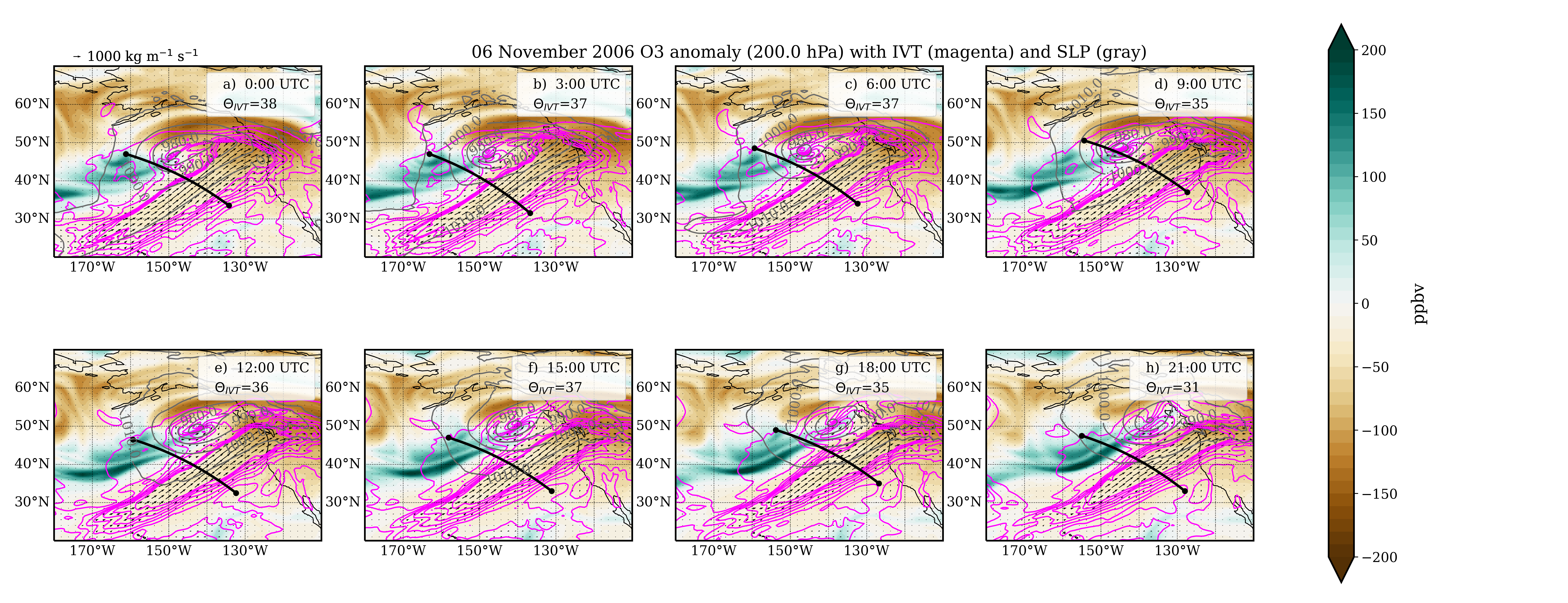
We further investigate the time series data for this AR event using the mixing ratios and IVT derived from MERRA-2. Beginning on 01 November 2006, our algorithm follows the evolution of nine atmospheric river events throughout the entire month by tracking the peak value of IVT at each 3-hour time step as outlined in Section 3.1. The algorithm begins tracking the early formation of this particular AR event on 04 November 2006 at 170∘ W and 32.5∘ N, and follows it until it completely diminishes on 08 November 2006, after making landfall on 06 November. We simultaneously track the peak anomaly as described in Section 3.2, as well as the separation between peak anomaly and peak IVT. Figure 3 shows shaded maps of the anomalous at 200 hPa in three-hourly time steps on 06 November 2006, with magenta IVT contours and gray sea level pressure (SLP1010 hPa) contours overlaid. This AR occurred in conjunction with an EC that can be identified via the low SLP. On this day, the peak values tracked by our algorithm are in excess of 120 ppbv for six out of the eight three-hour time steps, and the maximum excess for the entire day exceeds 240 ppbv.
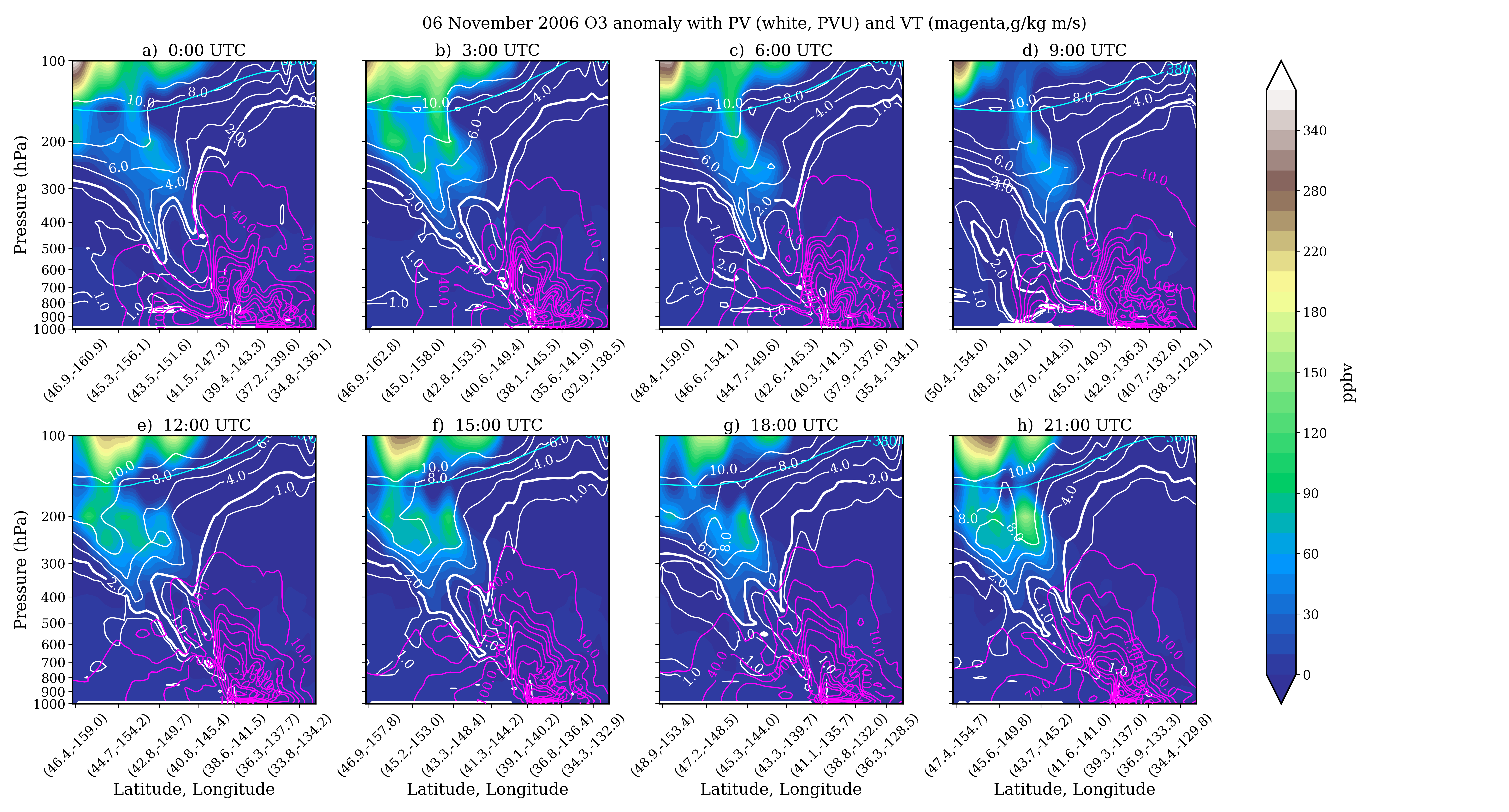
The thick, black line with two endpoints on each panel of Figure 3 approximately crosses through the location of the maximum anomaly and IVT, and is used to generate the vertical cross sections plotted in Figure 4. These cross-sections highlight the vertical structure of anomalous , PV (white), and water vapor transport (VT, magenta). The positive anomalies follow the PV contours indicative of tropopause folding upstream, poleward, and westward of the high water vapor flux of the AR in each time step. On 06 November, the dry intrusion bringing ozone-rich air reaches a pressure of at least 667 hPa as traced by these particular vertical cross sections (black lines in Figure 4). Using the \citeASker15 characterization of tropopause fold, this dry intrusion is classified as a medium fold with P 250 hPa. The tropopause remains lowered throughout the duration of the event and well after landfall. On 08 November 2006, two days after the AR made landfall, and while it was still detectable, the positive anomaly associated with the dry intrusion persisted with a significantly lowered dynamical tropopause at 480 hPa.
4.2 December 2010
As a second case study, we track all of the December 2010 AR events over the NE Pacific and quantify the associated dry intrusion and anomalies correlated with them. In this case, we also track the peak anomalies on the 400 hPa pressure layer in addition to the 200 hPa level. The 400 hPa pressure surface is insightful as the approximate height at which the water vapor transport intensity decreases to near zero and at which the positive anomalous remains consistently significant above the climatology. This pressure surface is also below the average level of the global extratropical dynamical tropopause, which is about 300 hPa, but varies significantly with latitude [Škerlak \BOthers. (\APACyear2014), Jaeglé \BOthers. (\APACyear2017)]. Over our region of interest and using the MERRA-2 data to determine the lower of the PV=2 or 380 K surface, we compute the average climatological dynamical tropopause to be 275 hPa.
ARs of December 2010 brought catastrophic consequences to the North American west coast. \citeARalp10 summarize the extreme precipitation due to two of these ARs’ transport of massive amounts of water vapor from the Pacific Ocean to the North American west coast resulting in as much as 250-670 mm of rainfall in mountainous areas, causing flooding, and also providing crucial snow pack between 10-12 December and 20-22 December. We track a total of nine ARs (by our algorithmic count) over the NE Pacific in December 2010, four of which were Cat 5 ARs (defined as having peak IVT1000 and duration 48 hours or peak IVT1250 kg m-1 s-1 and duration24 hours, [Ralph \BOthers. (\APACyear2019)]) that made landfall on the North American west coast.
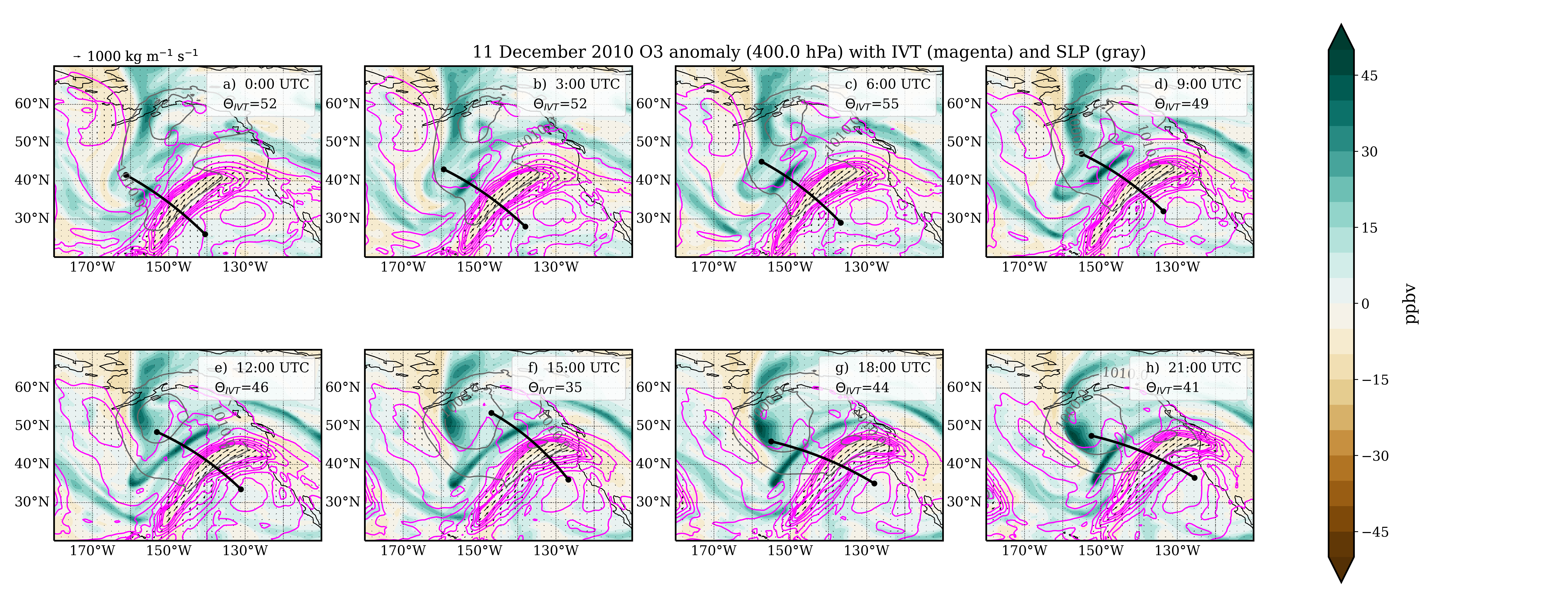
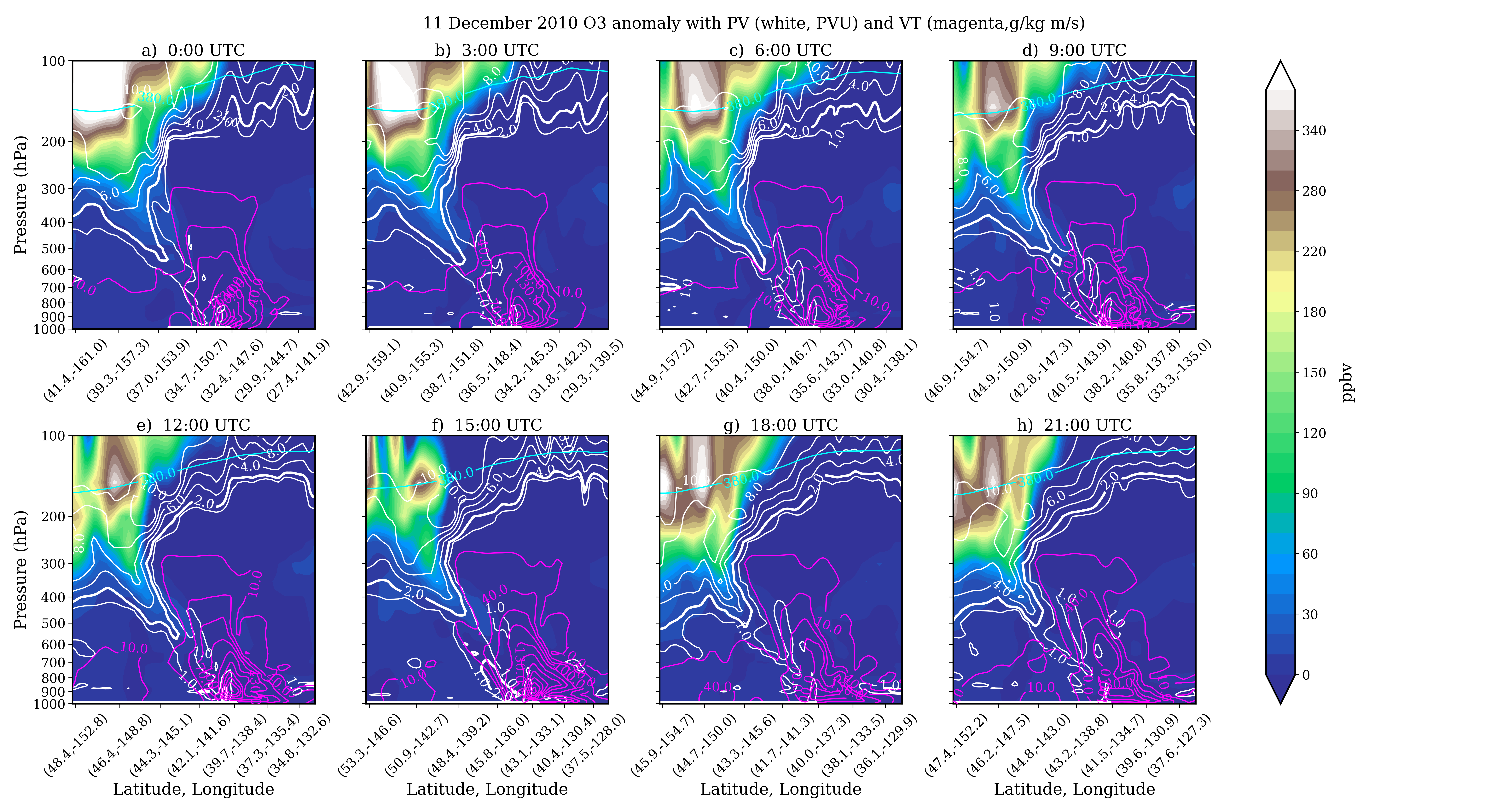
Figure 5 shows shaded maps of the anomalous at 400 hPa with magenta IVT contours and gray SLP overlaid in three-hour time steps for 11 December 2010, a day in which the peak IVT reached 1400 kg m-1 s-1. As in Figure 3, the black geodesic line crosses approximately through the location of the peak anomaly and IVT, and is used to generate the vertical cross sections shown in Figure 6. The peak anomalous at 400 hPa varies between 20-50 ppbv over the course of this AR event, which formed on 10 December 2010, made landfall on 11 December, and dissipated on 13 December after dropping in IVT to below 500 kg m-1 s-1 (Figure 7, red dots). The vertical cross section (Figure 6) reveals the tropopause fold via the PV contours (white) tilted eastward toward the AR, and it shows the positive anomalous (shading) coincident with the fold. At 200 hPa, the anomalous reaches over 300 ppbv. In Section 5.2 below, we estimate and discuss the total flux into the troposphere over the 4-day duration of this AR event.
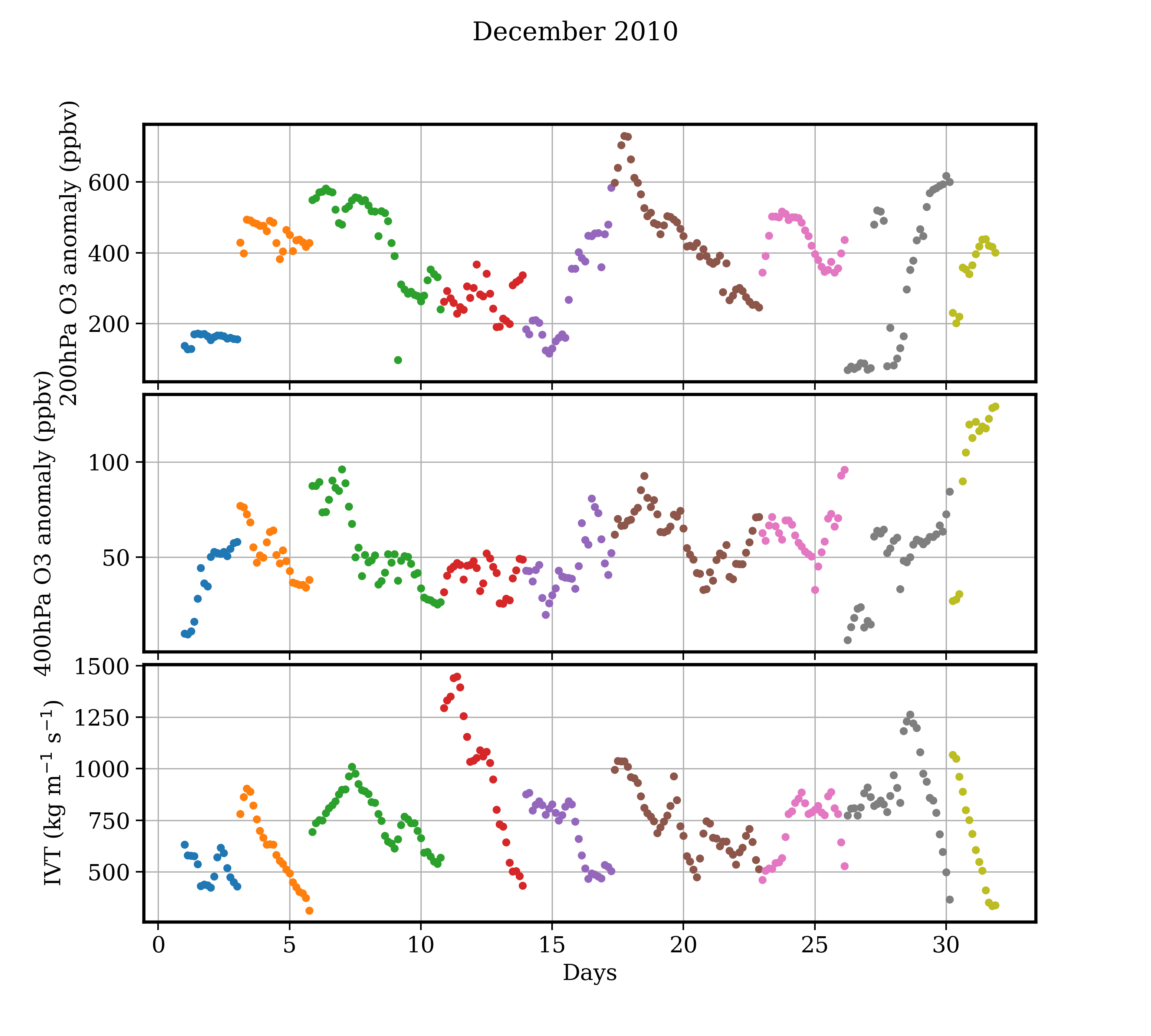
There were several other ARs of strong and extreme intensity that made landfall in December 2010, so we plot in Figure 7 the peak IVT and peak anomaly at each 3-hour time step. Each color indicates the tracking of an individual AR event until it dissipates, as defined by the binary tag catalog. While some correlation between IVT and anomaly peaks are discernible on short timescales, we find no statistically significant correlation in the time series across the entire month. We also test a lag correlation with no statistical significance. This lack of correlation may be due to spatial or temporal limitations of the algorithm. It may be that the choice of tracking individual anomalous points at 200 hPa and 400 hPa does not fully capture the dry intrusion depth. It is also possible that the correlated relationship between anomalous in dry intrusions following ARs is an average effect that depends on more global properties of the ARs, such as the entire duration of each event or its overall intensity. In the following sections, we systematically explore the correlation between average AR IVT and anomalous through examining composites binned according to the the magnitudes of their integrated vapor transport and quantifying the vertical structure of the anomalous , PV, and vapor transport of these composites.
5 Statistical Summary and Composite Results
We now explore the relationship between ARs and anomalies and dry intrusions statistically for all ARs occurring in the NE Pacific in December 2004-2014. While ARs occur all year, their numbers are greatest over the NE Pacific (U.S. West Coast Landfalling) during the Northern Hemisphere cold months (November through February) [Mundhenk \BOthers. (\APACyear2016)], so we focus on December. Assessment of anomalies associated with ARs indicates that the anomalies roughly trail behind the front of the AR, but the relative location depends on the direction of the AR (Figure 8). The morphology of the anomalies is often filamentary, like that of the ARs (e.g., Figure 1), but can also be more circular or clumped (e.g., Figure 5 top left).
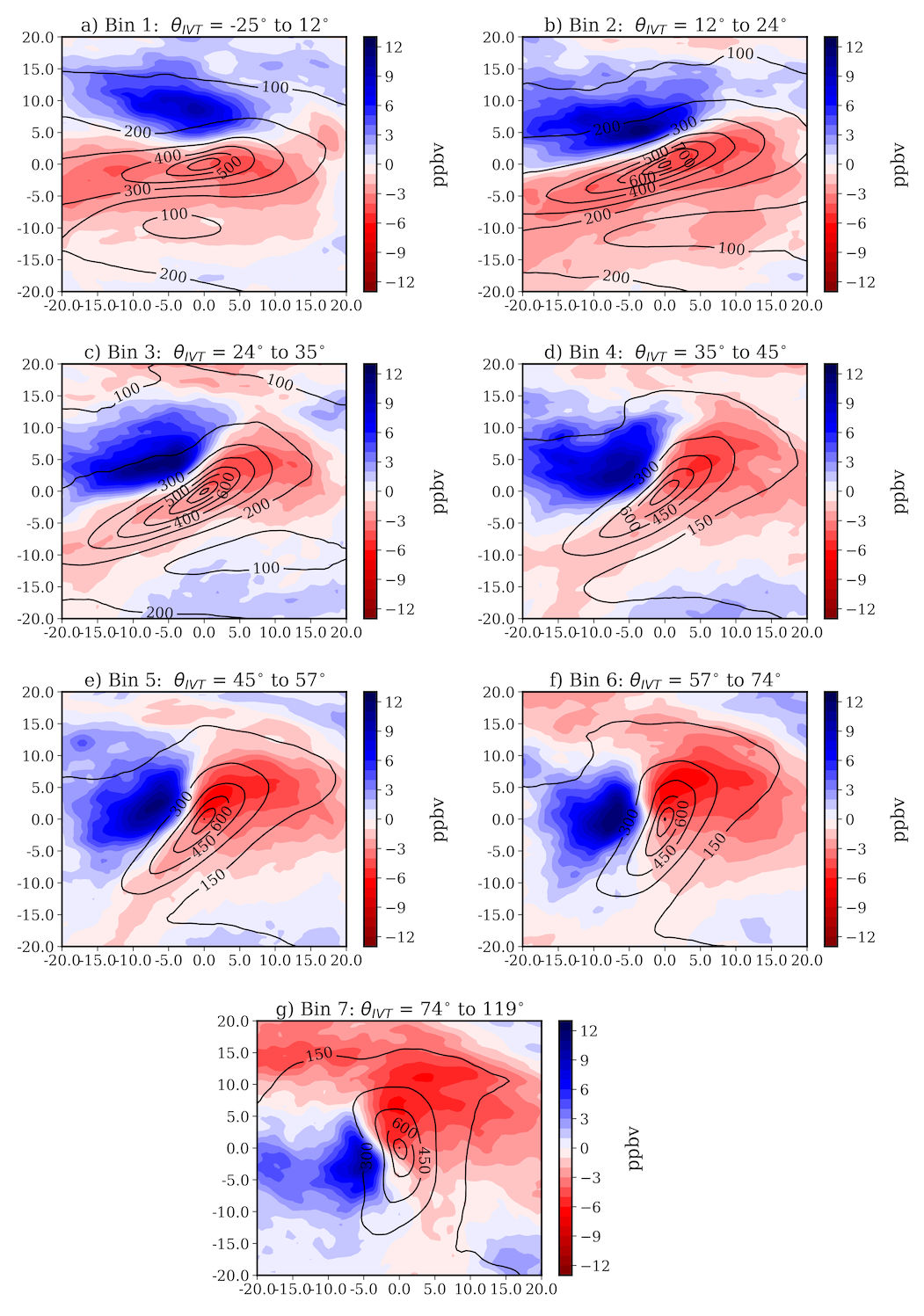
Figure 8 shows composite (average) anomaly (shading) at 400 hPa and IVT (black contours) for all three hour time steps in December 2004-2014 centered on the AR peak IVT for each time step and divided into seven bins of AR direction, as described in Section 3.3. The composites are oriented with x increasing in the east direction and y increasing in the poleward (north) direction, but the axes depict distance from the AR center (peak IVT location) in degrees. While many of the details of individual events have been averaged out due to latitudinal and longitudinal differences in the exact location of the anomalies relative to each AR center, the composites demonstrate the general direction of the anomalies associated with AR events. The positive anomalous occurs along the ARs’ long axis to the north/west, depending on the IVT angle, while negative anomalies are observed within the AR region (Figure 8), potentially as a result of troposphere-stratosphere transport (TST, see Figure 9 for more vertical information). The location of the peak value of anomaly relative to ARs traveling east/northeast is roughly north/northwest (Figure 8a-e), with the possibility of the maximum anomalous being a few degrees eastward of the peak IVT value if the direction of the IVT is east/southeast (ARs included in Figure 8a). For an AR traveling north or northeast, the anomaly lies directly west or southwest of the AR center (Figure 8e-g). We analyze only the positive anomalies that result from STT, and do not interpret the negative anomalies over the AR region due to the greater uncertainty of the MERRA-2 data in the lower troposphere. The STT is reliable as MERRA-2 adequately captures the upper tropospheric and lower stratospheric concentrations [Knowland \BOthers. (\APACyear2017)].
We see that the composites at 400 hPa have average peak anomalies ranging from 10-13 ppbv for all AR travel directions. For 95% of the individual AR time steps, the peak anomaly occurs between 500-1600 km from the center (or peak IVT) of the AR. In the composites, we find that the peak average anomaly occurs roughly 700-1000 km from the AR center, independent of the AR direction of travel. The only difference is the relative direction of the anomaly driven by the folding or lowering of the tropopause along the poleward or westward length of the ARs. While we use a different definition of anomaly than \citeAJaeg17, these anomalous amplitudes are commensurate in what they find for cyclone composites at the same pressure level.
5.1 Composite anomaly concentration as a function of AR IVT
We assess any correlation between the amplitude of positive anomaly and intensity of AR by further binning the ARs into two bins of peak IVT while still binning by direction of travel for the reasons described in the previous section. Using all of the AR IVTs across all directional bins, we define two bins: “low” for values of peak IVT in the first quartile and “high” for values of peak IVT in the fourth quartile of all event times that we track. These low and high bins correspond to all peak IVT less than 659 kg m-1 s-1 and greater than 1063 kg m-1 s-1, respectively. As a result, there are not necessarily the same number of AR IVTs in each bin because each bin may have a different IVT quartile ranges compared to the combined data set of all directions of ARs. These bins of peak IVT roughly separate the events into weak (Cat 1) and moderate (Cat 2) AR IVT values in the low bin and extreme (Cat 4) and exceptional (Cat 5) in the high bins, although in this part of the analysis we do not take into account duration nor the absolute maximum value of IVT over an entire event [<]for full categorization definitions see¿Ralp19. That is, time steps of a given AR event for which peak IVT is in the first quartile will be in the low bin and time steps of that same AR for which peak IVT is in the fourth quartile (if present) will be in the high bin.
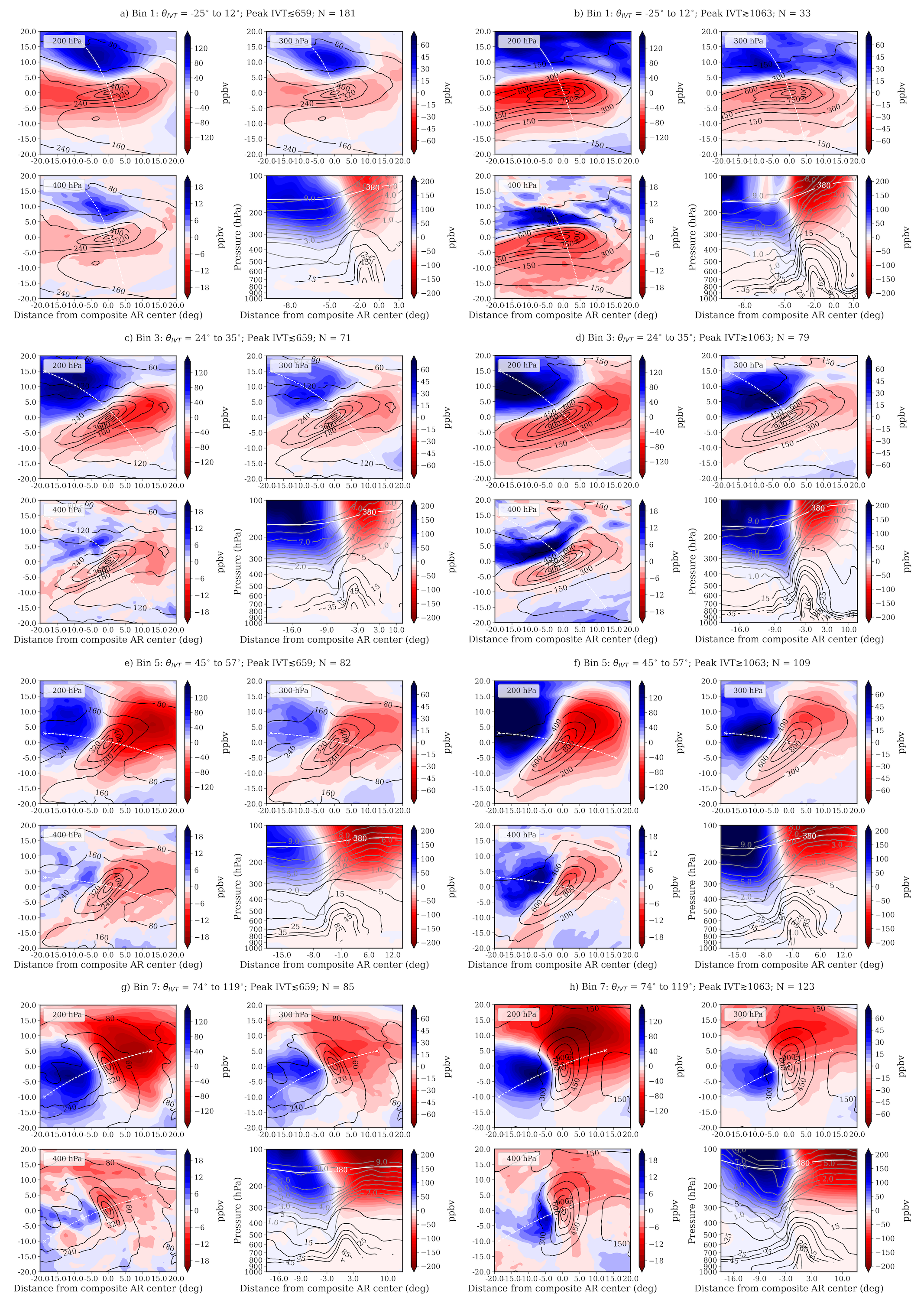
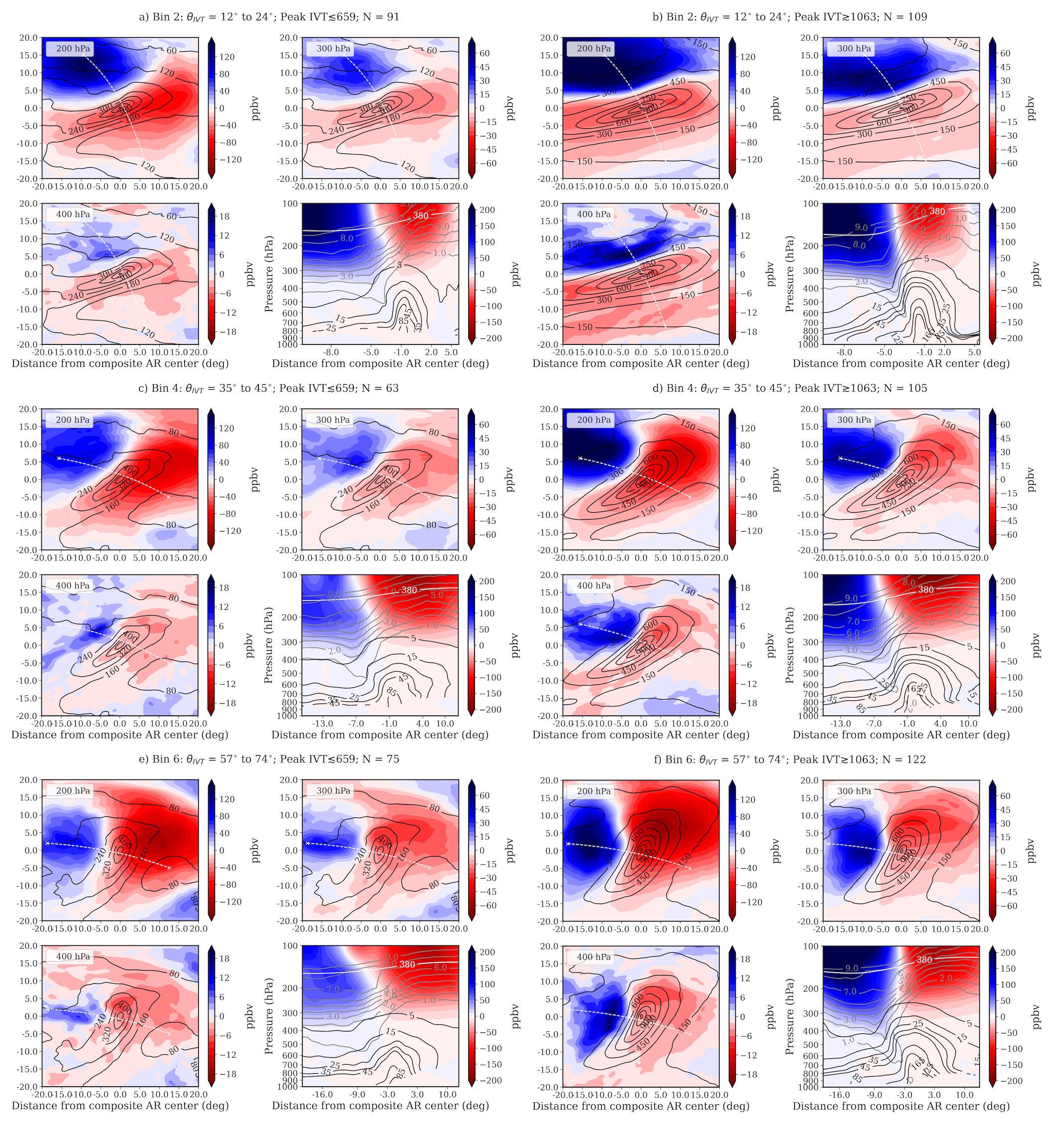
Figures 9 and 12 depict the three-dimensional structure of the anomalies associated with atmospheric rivers divided into bins by AR direction of travel and peak IVT values. Each two-by-two grid in the figures corresponds to the average anomalous at 200 (top left), 300 (top right), and 400 hPa (bottom left) pressure levels in latitude by longitude plotted as a function of distance from the center of AR peak IVT values. The vertical cross-section (bottom right) is computed across the white dashed line in the other three figures and spanning pressure levels 1000-100 hPa. Each of the two-row blocks in the figures corresponds to the seven bins of AR direction of travel, and the two columns of two by two blocks correspond to the two bins of peak IVT value (left: peak IVT 659 kg m-1 s-1; right: peak IVT 1059 kg m-1 s-1). The latitude by longitude cutouts at 200, 300, and 400 hPa help to demonstrate the dry intrusion’s breadth and the filamentary shape at 400 hPa along the length of the AR. The vertical (pressure level) cross-section (bottom right of each 2x2 grid, a-h) indicates the average depth of the dry intrusions and the west-to-east directionality as seen via the anomaly and the PV contours. The cross section is always shown from the approximate location of the maximum anomaly across the width of the AR. The PV intrusion is on average tilted toward the AR, regardless of AR direction of travel; we also saw this clearly in the case study events and time step cross sections in Figures 4 and 6. Once again, individual details of the lat x lon anomalies, and even more so, the depth of the dry intrusion, are averaged out by the slight differences in location of the intrusions and peak values relative to the center (peak IVT) of the AR at each time step. Here (Figure 9) we include only bins 1, 3, 5, and 7 as examples, and we placed the rest of the corresponding figures for bins 2, 4, and 6 in the appendix (Figure 12). Each bin tells a similar story regarding the division with respect to the two peak IVT bins, and more details are provided in Figure 10 for all of the directional bins.
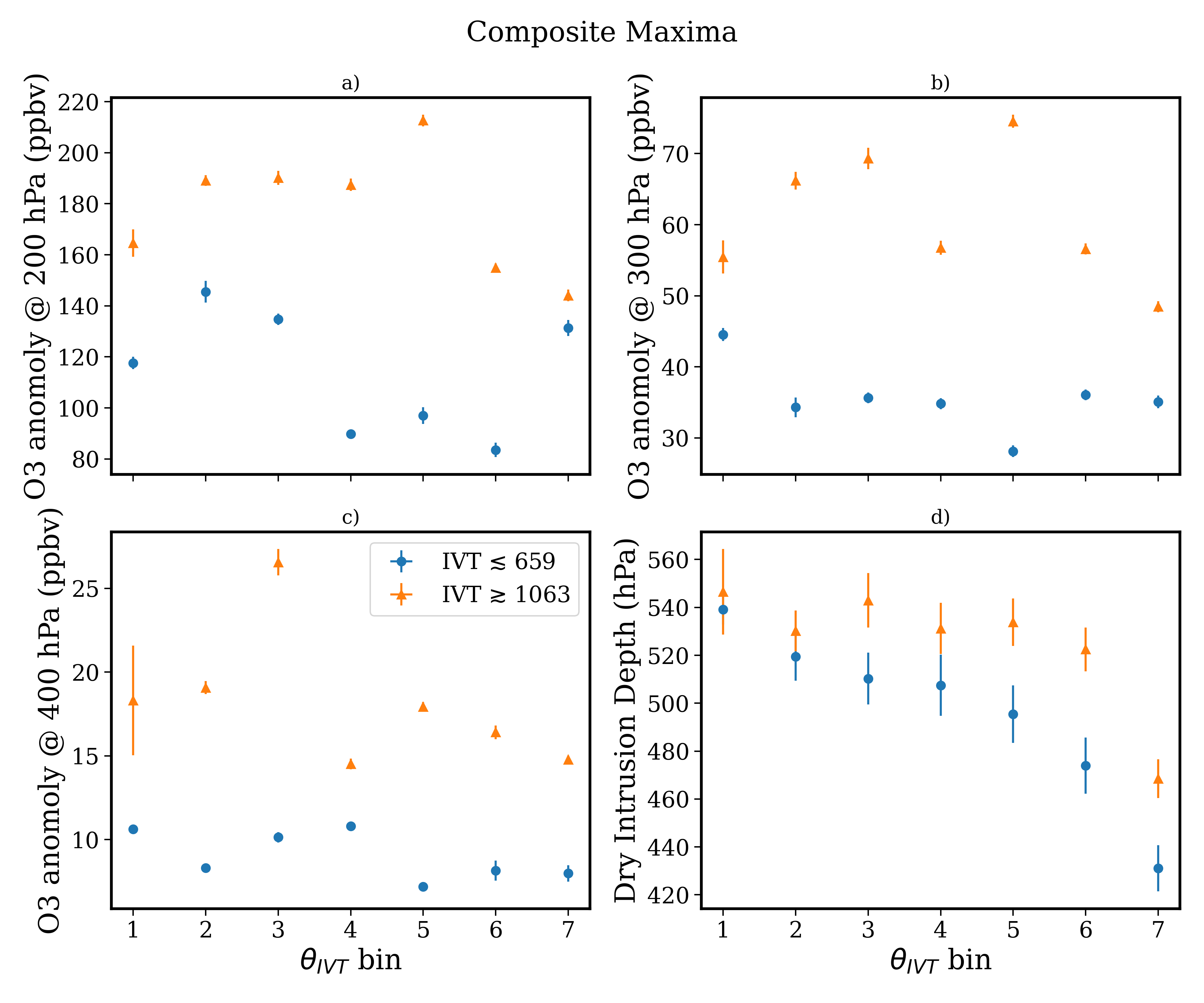
In Figure 10, the difference in magnitude of the anomalies in the low versus high peak IVT bins is clear: the low peak IVT bins correspond to smaller maximum anomalies in the composites at all pressure levels. At 400 hPa, the maximum value of the composite anomalous ranges between 14.50.3 to 25.50.8 ppbv for the peak IVT 1063 kg m-1 s-1 bin, and 7.10.3 to 10.80.3 ppbv in the low IVT bin. The uncertainties are the standard deviation of all means from 100 bootstrap realizations of the composites. Through this statistical analysis we observe that there is in fact a relationship between anomalous and AR intensity.
We investigate whether the anomalous concentrations are driven by the depth of the dry intrusions by tracking the maximum pressure reached by the PV=2 contour within the dry intrusion for each time step of each AR (see Section 3.2 for intrusion identification). In the lower right panel of Figure 10, we plot the average depth of the dry intrusions computed for the low versus high peak IVT bins. The uncertainties reflect the standard error on the mean. We find that while the high IVT bin dry intrusions are on average deeper, there is not a clear statistical divide for all bins of . A two-sided Kolmogorov–Smirnov test on the entire distributions of dry intrusion depths for all bins of separated only into bins of low (first quartile) and high (fourth quartile) IVT produces a p-value of 0.025, rejecting the null hypothesis that the samples are drawn from the same distribution. Performing this test on each bin, we reject the null hypothesis for bins 3, 5, 6, and 7; however, this test does not account for the uncertainty in the bins. Again, averaging according to peak IVT value over all 3 hour time steps may be detracting from the details of the individual events. The downward trend in average depth indicates that tracing the dry intrusion along an eastward travelling AR yields, on average, deeper intrusion events; while an east-west cross section cutting through northward ARs results in a more shallow tracing of the dry intrusion. This is likely explained by the orientation of the cold front with respect to AR direction of travel.
Another way to assess the relationship of ARs to the depth of associated dry intrusion events is in the distribution of depths in relation to all AR events. Over the course of the eleven Decembers studied in this work, we track 138 AR events. Of these, 39 of them are connected to a dry intrusion that reaches below 700 hPa in at least one of the time steps throughout its duration; this amounts to 28.3% of all AR events we track. Our algorithm for tracking the tropopause folding or lowering ensures the tracking of the PV=2 contour connected to the stratosphere and not part of a cutoff (Section 3.2), and we visually inspected this set of ARs to ensure the depth of the dry intrusions reach at least 700 hPa. The percentage of the ARs connected to dry intrusions that are classified as deep (with P350 hPa, [Škerlak \BOthers. (\APACyear2015)]) in at least one time step for the duration of the AR event is 79.7%. If we compute the same statistic for all times in which the peak IVT is in the first quartile (low IVT bin), this includes a total of 116 ARs for which 7.7% and 46.5% of them are connected to dry intrusions that in at least one time step reach below 700 hPa and are classified as deep, respectively. For the fourth quartile (high IVT bin) case, there are a total of 81 ARs for which the below 700 hPa and deep classifications are 16% and 64.2%. This total AR event analysis indicates that a larger fraction of the high IVT bin ARs are connected to deeper dry intrusions and those which more frequently reach blow 700 hPa.
5.2 Composite STT flux as a function of AR IVT and in comparison to other work
With the MERRA-2 data products, we quantify the total flux of from the stratosphere into the troposphere (via STT) in relation to ARs following the methods described in Section 3.2. We do not attempt to compute the TST since the MERRA-2 data has larger bias in the upper troposphere as discussed in Section 2 [Wargan \BOthers. (\APACyear2017)]. Assessing the percentage of that reaches our constraining depth in the dry intrusion and is then pulled back up into the stratosphere is beyond the scope of this work, and thus, we advise careful consideration of these flux constraints. For the purpose of this exercise of comparing total flux in dry intrusion events associated with ARs to those from ECs, and other STT events more generally, we assume that the stratospheric within the dry intrusion as defined by these PV limits is irreversibly mixed into the troposphere [Jaeglé \BOthers. (\APACyear2017), Stohl \BOthers. (\APACyear2003), Rood \BOthers. (\APACyear1997), Lamarque \BBA Hess (\APACyear1994)].
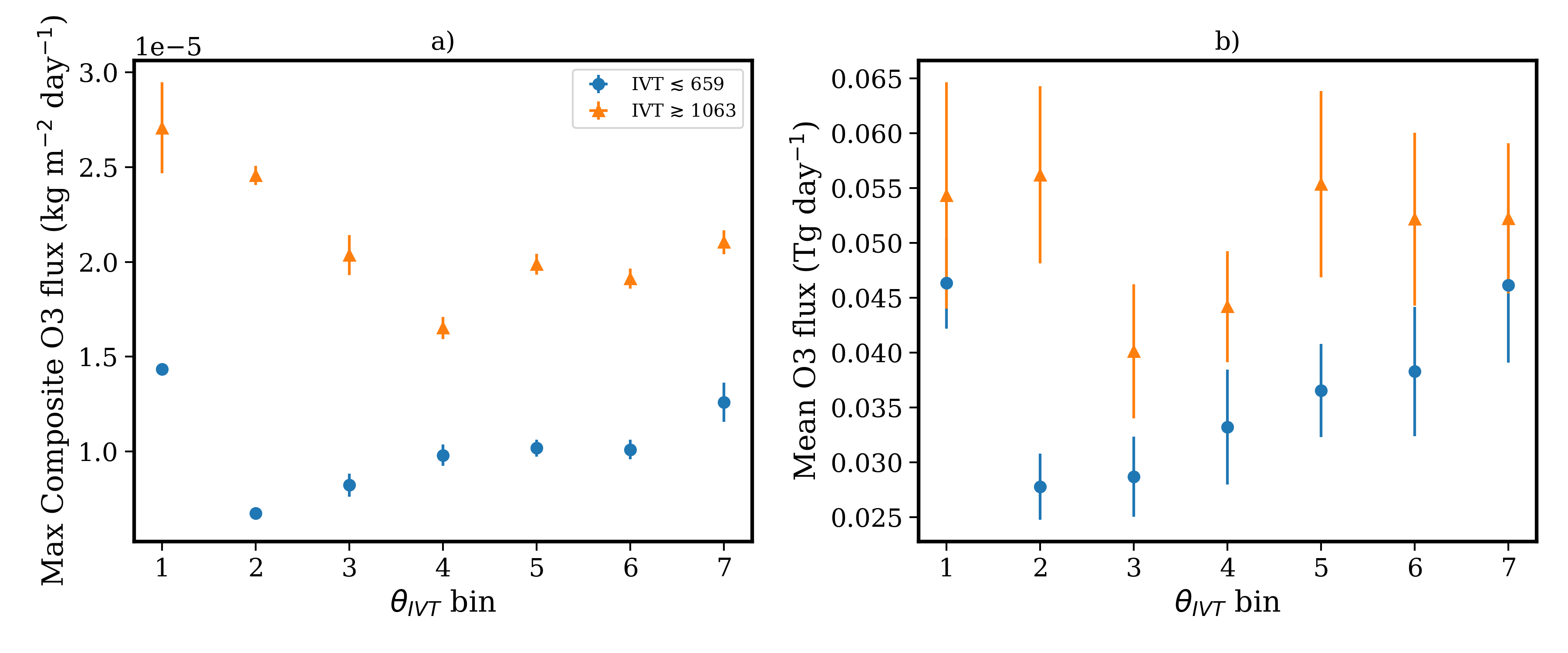
Figure 11, left, shows the maximum composite flux (left, kg m-2 day-1) as a function of for the high and low IVT bins, in orange and blue, respectively computed for all ARs that we track in December 2004-2014. The uncertainties are the standard deviation of the maximum of all means from 100 bootstrap realizations of the composites. Latitude x longitude composites of flux centered on the AR peak IVT locations for dry intrusions with depth P350 hPa, divided into bins of direction and peak IVT, are plotted in the appendix, Figures 13 and 14. The right panel of Figure 11 shows the average total flux (Tg day-1) integrated over the 20∘ lat x 20∘ lon area around the peak IVT for each time step of the ARs and averaged over the total number of days in each bin. These area-integrated fluxes are computed individually for each time step of each AR in order to properly account for the distance covered with respect to latitude over the total area as the ARs move. In the IVT659 kg m-1 s-1 bins, we find average fluxes ranging from 0.0280.003 to 0.0460.007 Tg day-1, and in the IVT1063 kg m-1 s-1 bins, the average fluxes range from 0.040.006 to 0.0560.008 Tg day-1. The uncertainties shown in the right-hand panel of Figure 11 reflect the standard error on the mean, whereas the full range of area integrated fluxes for all ARs span 0.002-0.21 Tg day-1. Considering all bins, we do find a measurable difference in the total area integrated flux for our two bins of IVT, with lower intensity events resulting in lower STT flux. We performed the same computation for the case study event on 10-12 December 2010, and found an average flux of 0.15 Tg day-1. All of these values are consistent with means and individual case studies for ECs: \citeAJaeg17 find mean STT flux from cyclones in the DJF season to be 0.075 Tg day-1, with total values ranging from 0.01 to 0.24 Tg day-1 and a strong dependence on 300 hPa wind speed; Other EC-associated STT flux measurements range from 0.01-0.15 Tg day-1 for a variety of individual events as well as averages computed via ground-based lidar measurements and Lagrangian trajectories [Ancellet \BOthers. (\APACyear1991), Lamarque \BBA Hess (\APACyear1994), Ebel \BOthers. (\APACyear1996), Beekmann \BOthers. (\APACyear1997), Cooper \BOthers. (\APACyear2004), Kuang \BOthers. (\APACyear2012)].
While a complete assessment of NH STT flux in connection to AR occurrences in contract to that in non-AR occurrences is beyond the scope of this paper, we can provide an estimation based on the others’ climatological STT flux as a function of geography and time, namely we use the results from \citeASker14. \citeASker14 Figure 18a shows the monthly STT flux for the Northern Hemisphere averaged from 1979-2011. From this figure, the December average is approximately 142 Tg month-1. If we consider the average STT flux from AR events that we track of 0.0580.003 Tg day-1 and multiply by 31 days per month in December, this amounts to 1.800.09 Tg month-1, or between 132% of the total December NH STT flux. Our method here only tracks one AR at a time through its lifetime over the NE Pacific. In order to compare the AR dry intrusion contribution directly to the total STT flux in the NH, we would need to track all ARs in the NH simultaneously – a specific task that we reserve for future work. We give a rough approximation by considering that 4-5 ARs occur simultaneously around the globe [Ralph \BBA Dettinger (\APACyear2011)]. If half of these are active in the Northern Hemisphere, we approximate that the total STT flux due to dry intrusions following ARs is 3.6-4.5 Tg month-1 for December; or as much as 32% of the total NH STT flux.
Furthermore, \citeAJaeg17 find similar mean fluxes per cyclone to our average value, 0.057 Tg day-1. Summing over all NH cyclones (4-6 per day), they reported daily mean total STT flux from all NH cyclones to range from 0.1-0.5 Tg day-1 with a total contribution to the annual flux of 119 Tg year-1, which suggest the EC dry intrusion STT flux makes up 42% of all annual NH STT flux [<]281 Tg year-1,¿Jaeg17. Given the strong link between the occurrence of ECs and ARs, some fraction of the flux in dry intrusions associated with each of these phenomena is overlapping; thus these are not independent results. Though ARs coincide with an EC 82% of the time in the North Pacific, AR location and duration cannot be determined from the EC [Zhang \BOthers. (\APACyear2019)]. In the North Atlantic, for example, \citeASode13 find that the lifetime of a single AR can span several ECs. Thus, disentangling the STT flux contribution in dry intrusions associated with ECs and ARs, respectively, is a complex task.
6 Summary and Conclusion
We have demonstrated for the first time positive anomalies in the troposphere associated with atmospheric river events over the NE Pacific ocean for December 2004-2014. These anomalies result from intrusions of dry, ozone-rich stratospheric air into the troposphere via STT following to the north/west of the AR’s travel direction. While ARs are associated with ECs (ECs) 82% of the time, the exact location, duration, and intensity cannot be determined from the EC [Zhang \BOthers. (\APACyear2019)]. We thus demonstrate the value in assessing the general location, duration, and magnitude of the anomalies connected to the AR events.
Individual case studies of extreme AR events in November 2006 and December 2010 show STT of in dry intrusions with excess concentrations compared to the climatology reaching hundreds of parts per billion at 200 hPa near the tropopause, and consistently in excess of 50 ppbv in the upper troposphere at 400 hPa (Figure 7). Composites for all AR events in December 2004-2014 show anomalies in the upper troposphere within dry intrusions span up to the full average length of all ARs within a given (direction of AR) bin. Moreover, the average amplitude of excess concentration at 400 hPa and total flux in the dry intrusions increases with increasing AR IVT. For all December AR events included in this analysis, the associated dry intrusion flux per AR event ranges from 0.001 to 0.16 Tg day-1, with a median of 0.06 Tg day-1. If we assume that the average flux is representative of all ARs across the globe at a given time, then this would indicate the dry intrusion STT flux connected to ARs could be responsible for up to 32% of the total NH STT flux for December [Škerlak \BOthers. (\APACyear2014), Jaeglé \BOthers. (\APACyear2017)].
In light of the projected increase in both intensity and AR-day frequency of ARs with climate change [Dettinger (\APACyear2011), Espinoza \BOthers. (\APACyear2018), X. Huang \BOthers. (\APACyear2020), Payne \BOthers. (\APACyear2020), Rhoades \BOthers. (\APACyear2021)], quantifying and closely monitoring dynamically-related phenomena such as this is critical. Our work here implies that the increased intensity and/or frequency of ARs may also bring increased STT flux in the warming future. The overall levels of tropospheric concentration as a result are dependent on a thorough assessment of the TST, and residence times need to be fully considered in conjunction. The primary impact, however, of AR-associated dry intrusions is on the upper troposphere, which is highly consequential for the outgoing longwave radiation [Bowman \BOthers. (\APACyear2013), Doniki \BOthers. (\APACyear2015)]. In fact, the longwave radiative effect may be most sensitive to concentrations in the upper troposphere [Lacis \BOthers. (\APACyear1990), Worden \BOthers. (\APACyear2011)], thus emphasizing the importance of quantifying UT/LS concentrations and STT flux from all sources.
Appendix A Additional Composite Figures
Here we include important, additional figures that are not vital for the main text. Figure 12 exemplifies the extent of composite anomalous concentrations as a function of pressure at 200 (top left), 300 (top right), and 400 hPa (bottom left) for AR bins 2, 4, and 6. These are the same as Figure 9 in the main text, but for the other three bins in AR direction of travel. AR directions are reported in the titles of each figure. The bottom right panel in each of the 2x2 figures indicates the vertical cross section over the white dashed line in each of the other three figures, thus providing three dimensional information for the anomalous concentrations and the average vertical transport of the Atmospheric Rivers’ water vapor content. Also indicated is the average potential vorticity contours (gray) and the 380 K isosurface (white). The left-hand set of 2x2 figures are for ARs with peak IVT 659 kg m-1 s-1 (in the first quartile) and the right-hand column is for those with peak IVT in the fourth quartile. These figures are provided here in the appendix for completeness and to save space, and reflect parallel information as the other four bins. The Composite maxima values are summarized in Figure 5 in the main text.
Figures 13 and 14 show the flux for ARs with dry intrusion depths with pressure greater than 350 hPa for ARs in bins of and peak IVT (low and high for Figures 13 and 14, respectively). The figures demonstrate the smaller flux for low IVT ARs, and larger flux for the more intense As. The statistical summary for all events are plotted in Figure 11.


Open Research
Data from the Modern-Era Retrospective analysis for Research and Applications, Version 2 instantaneous monthly [Global Modeling and Assimilation Office (GMAO) (\APACyear2015\APACexlab\BCnt2)] and 3-hourly [Global Modeling and Assimilation Office (GMAO) (\APACyear2015\APACexlab\BCnt1)] were used in the creation of this manuscript. We also use profiles from the Ozone Monitoring Instrument aboard the Aura spacecraft. The profiles and instructions for using them are available through the Aura validation center: https://avdc.gsfc.nasa.gov/pub/data/satellite/Aura/OMI/V03/L2/OMPROFOZ/. All ARTMIP Tier 1 catalogs used in this work are available via the Climate Data Gateway at NCAR (DOI: https://doi.org/10.5065/D62R3QFS). All data processing and plotting was done using Python version 3.8.12 installed with Miniconda3 [\APACcitebtitleAnaconda Software Distribution (\APACyear2020)]. For calculation of vertical cross sections, we use the publicly available package MetPy [Unidata (\APACyear2020)].
Acknowledgements.
The authors thank the reviewers of for their valuable feedback. We are grateful to Emma Knowland for her insightful comments, which significantly improved the content and logical flow of this manuscript. The authors were supported by the NASA OMI core science team Grant #80NSSC21K0177 and the NASA Making Earth System Data Records for Use in Research Environments (MEaSUREs) Grant #80NSSC18M0091. K.R.H. acknowledges the support from the Schmidt Science Fellows, in partnership with the Rhodes Trust for the completion of this work. Some computations for this paper were conducted at the Smithsonian High Performance Cluster (SI/HPC), Smithsonian Institution (https://doi.org/10.25572/SIHPC). We also acknowledge the use of the ARTMIP project catalogs. ARTMIP is a grass-roots community effort and includes a collection of international researchers from universities, laboratories, and agencies. Co-chairs and committee members include Jonathan Rutz, Christine Shields, L. Ruby Leung, F. Martin Ralph, and Michael Wehner, Ashley Payne, and Travis O’Brien. Details on catalogues developers can be found on the ARTMIP website. ARTMIP has received support from the US Department of Energy Office of Science Biological and Environmental Research (BER) as part of the Regional and Global Climate Modeling program, and the Center for Western Weather and Water Extremes (CW3E) at Scripps Institute for Oceanography at the University of California, San Diego.References
- Abalos \BOthers. (\APACyear2020) \APACinsertmetastarabal20{APACrefauthors}Abalos, M., Orbe, C., Kinnison, D\BPBIE., Plummer, D., Oman, L\BPBID., Jöckel, P.\BDBLDameris, M. \APACrefYearMonthDay2020. \BBOQ\APACrefatitleFuture trends in stratosphere-to-troposphere transport in CCMI models Future trends in stratosphere-to-troposphere transport in ccmi models.\BBCQ \APACjournalVolNumPagesAtmospheric Chemistry and Physics20116883–6901. {APACrefURL} https://acp.copernicus.org/articles/20/6883/2020/ {APACrefDOI} 10.5194/acp-20-6883-2020 \PrintBackRefs\CurrentBib
- \APACcitebtitleAnaconda Software Distribution (\APACyear2020) \APACinsertmetastarconda\APACrefbtitleAnaconda Software Distribution. Anaconda software distribution. \APACrefYearMonthDay2020. \APACaddressPublisherAnaconda Inc. {APACrefURL} https://docs.conda.io/projects/miniconda \PrintBackRefs\CurrentBib
- Ancellet \BOthers. (\APACyear1991) \APACinsertmetastarAnce91{APACrefauthors}Ancellet, G., Pelon, J., Beekman, M., Papayannis, A.\BCBL \BBA Megie, G. \APACrefYearMonthDay1991\APACmonth12. \BBOQ\APACrefatitleGround-based lidar studies of ozone exchanges between the stratosphere and the troposphere Ground-based lidar studies of ozone exchanges between the stratosphere and the troposphere.\BBCQ \APACjournalVolNumPagesJournal of Geophysical Research96D1222,401-22,421. {APACrefDOI} 10.1029/91JD02385 \PrintBackRefs\CurrentBib
- Beekmann \BOthers. (\APACyear1997) \APACinsertmetastarBeek97{APACrefauthors}Beekmann, M., Ancellet, G., Blonsky, S., De Muer, D., Ebel, A., Elbern, H.\BDBLVan Haver, P. \APACrefYearMonthDay1997\APACmonth01. \BBOQ\APACrefatitleRegional and Global Tropopause Fold Occurrence and Related Ozone Flux Across the Tropopause Regional and Global Tropopause Fold Occurrence and Related Ozone Flux Across the Tropopause.\BBCQ \APACjournalVolNumPagesJournal of Atmospheric Chemistry2829-44. {APACrefDOI} 10.1023/A:1005897314623 \PrintBackRefs\CurrentBib
- Bowman \BOthers. (\APACyear2013) \APACinsertmetastarBowm13{APACrefauthors}Bowman, K\BPBIW., Shindell, D\BPBIT., Worden, H\BPBIM., Lamarque, J\BPBIF., Young, P\BPBIJ., Stevenson, D\BPBIS.\BDBLWorden, J\BPBIR. \APACrefYearMonthDay2013. \BBOQ\APACrefatitleEvaluation of ACCMIP outgoing longwave radiation from tropospheric ozone using TES satellite observations Evaluation of accmip outgoing longwave radiation from tropospheric ozone using tes satellite observations.\BBCQ \APACjournalVolNumPagesAtmospheric Chemistry and Physics1384057–4072. {APACrefURL} https://acp.copernicus.org/articles/13/4057/2013/ {APACrefDOI} 10.5194/acp-13-4057-2013 \PrintBackRefs\CurrentBib
- Browning (\APACyear1997) \APACinsertmetastarBrow97{APACrefauthors}Browning, K\BPBIA. \APACrefYearMonthDay1997\APACmonth12. \BBOQ\APACrefatitleThe dry intrusion perspective of extra‑tropical cyclone development The dry intrusion perspective of extra‑tropical cyclone development.\BBCQ \APACjournalVolNumPagesMeteorological Applications44317-324. {APACrefDOI} 10.1017/S1350482797000613 \PrintBackRefs\CurrentBib
- Collow \BOthers. (\APACyear2020) \APACinsertmetastarColl20{APACrefauthors}Collow, A\BPBIB\BPBIM., Mersiovsky, H.\BCBL \BBA Bosilovich, M\BPBIG. \APACrefYearMonthDay2020. \BBOQ\APACrefatitleLarge-Scale Influences on Atmospheric River–Induced Extreme Precipitation Events along the Coast of Washington State Large-scale influences on atmospheric river–induced extreme precipitation events along the coast of washington state.\BBCQ \APACjournalVolNumPagesJournal of Hydrometeorology2192139 - 2156. {APACrefURL} https://journals.ametsoc.org/view/journals/hydr/21/9/jhmD190272.xml {APACrefDOI} https://doi.org/10.1175/JHM-D-19-0272.1 \PrintBackRefs\CurrentBib
- Collow \BOthers. (\APACyear2022) \APACinsertmetastarColl22{APACrefauthors}Collow, A\BPBIB\BPBIM., Shields, C\BPBIA., Guan, B., Kim, S., Lora, J\BPBIM., McClenny, E\BPBIE.\BDBLWehner, M. \APACrefYearMonthDay2022. \BBOQ\APACrefatitleAn Overview of ARTMIP’s Tier 2 Reanalysis Intercomparison: Uncertainty in the Detection of Atmospheric Rivers and Their Associated Precipitation An overview of artmip’s tier 2 reanalysis intercomparison: Uncertainty in the detection of atmospheric rivers and their associated precipitation.\BBCQ \APACjournalVolNumPagesJournal of Geophysical Research: Atmospheres1278e2021JD036155. {APACrefURL} https://agupubs.onlinelibrary.wiley.com/doi/abs/10.1029/2021JD036155 \APACrefnotee2021JD036155 2021JD036155 {APACrefDOI} https://doi.org/10.1029/2021JD036155 \PrintBackRefs\CurrentBib
- Cooper \BOthers. (\APACyear2004) \APACinsertmetastarCoop04{APACrefauthors}Cooper, O., Forster, C., Parrish, D., Dunlea, E., Hübler, G., Fehsenfeld, F.\BDBLHorowitz, L. \APACrefYearMonthDay2004. \BBOQ\APACrefatitleOn the life cycle of a stratospheric intrusion and its dispersion into polluted warm conveyor belts On the life cycle of a stratospheric intrusion and its dispersion into polluted warm conveyor belts.\BBCQ \APACjournalVolNumPagesJournal of Geophysical Research109D23. {APACrefURL} https://agupubs.onlinelibrary.wiley.com/doi/abs/10.1029/2003JD004006 {APACrefDOI} https://doi.org/10.1029/2003JD004006 \PrintBackRefs\CurrentBib
- Dacre \BOthers. (\APACyear2015) \APACinsertmetastardacr15{APACrefauthors}Dacre, H\BPBIF., Clark, P\BPBIA., Martinez-Alvarado, O., Stringer, M\BPBIA.\BCBL \BBA Lavers, D\BPBIA. \APACrefYearMonthDay2015. \BBOQ\APACrefatitleHow Do Atmospheric Rivers Form? How do atmospheric rivers form?\BBCQ \APACjournalVolNumPagesBulletin of the American Meteorological Society9681243 - 1255. {APACrefURL} https://journals.ametsoc.org/view/journals/bams/96/8/bams-d-14-00031.1.xml {APACrefDOI} 10.1175/BAMS-D-14-00031.1 \PrintBackRefs\CurrentBib
- Danielsen (\APACyear1968) \APACinsertmetastarDani68{APACrefauthors}Danielsen, E\BPBIF. \APACrefYearMonthDay1968\APACmonth05. \BBOQ\APACrefatitleStratospheric-Tropospheric Exchange Based on Radioactivity, Ozone and Potential Vorticity. Stratospheric-Tropospheric Exchange Based on Radioactivity, Ozone and Potential Vorticity.\BBCQ \APACjournalVolNumPagesJournal of Atmospheric Sciences253502-518. {APACrefDOI} 10.1175/1520-0469(1968)025<0502:STEBOR>2.0.CO;2 \PrintBackRefs\CurrentBib
- Dee \BOthers. (\APACyear2011) \APACinsertmetastarDee11{APACrefauthors}Dee, D\BPBIP., Uppala, S\BPBIM., Simmons, A\BPBIJ., Berrisford, P., Poli, P., Kobayashi, S.\BDBLVitart, F. \APACrefYearMonthDay2011. \BBOQ\APACrefatitleThe ERA-Interim reanalysis: configuration and performance of the data assimilation system The era-interim reanalysis: configuration and performance of the data assimilation system.\BBCQ \APACjournalVolNumPagesQuarterly Journal of the Royal Meteorological Society137656553-597. {APACrefURL} https://rmets.onlinelibrary.wiley.com/doi/abs/10.1002/qj.828 {APACrefDOI} https://doi.org/10.1002/qj.828 \PrintBackRefs\CurrentBib
- Dettinger (\APACyear2011) \APACinsertmetastarDett11b{APACrefauthors}Dettinger, M. \APACrefYearMonthDay2011. \BBOQ\APACrefatitleClimate Change, Atmospheric Rivers, and Floods in California – A Multimodel Analysis of Storm Frequency and Magnitude Changes1 Climate change, atmospheric rivers, and floods in california – a multimodel analysis of storm frequency and magnitude changes1.\BBCQ \APACjournalVolNumPagesJAWRA Journal of the American Water Resources Association473514-523. {APACrefURL} https://onlinelibrary.wiley.com/doi/abs/10.1111/j.1752-1688.2011.00546.x {APACrefDOI} https://doi.org/10.1111/j.1752-1688.2011.00546.x \PrintBackRefs\CurrentBib
- de Vries (\APACyear2021) \APACinsertmetastardeVr21{APACrefauthors}de Vries, A\BPBIJ. \APACrefYearMonthDay2021. \BBOQ\APACrefatitleA global climatological perspective on the importance of Rossby wave breaking and intense moisture transport for extreme precipitation events A global climatological perspective on the importance of rossby wave breaking and intense moisture transport for extreme precipitation events.\BBCQ \APACjournalVolNumPagesWeather and Climate Dynamics21129–161. {APACrefURL} https://wcd.copernicus.org/articles/2/129/2021/ {APACrefDOI} 10.5194/wcd-2-129-2021 \PrintBackRefs\CurrentBib
- Doniki \BOthers. (\APACyear2015) \APACinsertmetastarDoni15{APACrefauthors}Doniki, S., Hurtmans, D., Clarisse, L., Clerbaux, C., Worden, H\BPBIM., Bowman, K\BPBIW.\BCBL \BBA Coheur, P\BHBIF. \APACrefYearMonthDay2015. \BBOQ\APACrefatitleInstantaneous longwave radiative impact of ozone: an application on IASI/MetOp observations Instantaneous longwave radiative impact of ozone: an application on iasi/metop observations.\BBCQ \APACjournalVolNumPagesAtmospheric Chemistry and Physics152212971–12987. {APACrefURL} https://acp.copernicus.org/articles/15/12971/2015/ {APACrefDOI} 10.5194/acp-15-12971-2015 \PrintBackRefs\CurrentBib
- Ebel \BOthers. (\APACyear1996) \APACinsertmetastarEbel96{APACrefauthors}Ebel, A., Elbern, H., Hendricks, J.\BCBL \BBA Meyer, R. \APACrefYearMonthDay1996\APACmonth01. \BBOQ\APACrefatitleStratosphere-Troposphere Exchange and Its Impact on the Structure of the Lower Stratosphere. Stratosphere-Troposphere Exchange and Its Impact on the Structure of the Lower Stratosphere.\BBCQ \APACjournalVolNumPagesJournal of Geomagnetism and Geoelectricity481135-144. {APACrefDOI} 10.5636/jgg.48.135 \PrintBackRefs\CurrentBib
- Eiras-Barca \BOthers. (\APACyear2018) \APACinsertmetastarEira18{APACrefauthors}Eiras-Barca, J., Ramos, A\BPBIM., Pinto, J\BPBIG., Trigo, R\BPBIM., Liberato, M\BPBIL\BPBIR.\BCBL \BBA Miguez-Macho, G. \APACrefYearMonthDay2018. \BBOQ\APACrefatitleThe concurrence of atmospheric rivers and explosive cyclogenesis in the North Atlantic and North Pacific basins The concurrence of atmospheric rivers and explosive cyclogenesis in the north atlantic and north pacific basins.\BBCQ \APACjournalVolNumPagesEarth System Dynamics9191–102. {APACrefURL} https://esd.copernicus.org/articles/9/91/2018/ {APACrefDOI} 10.5194/esd-9-91-2018 \PrintBackRefs\CurrentBib
- Espinoza \BOthers. (\APACyear2018) \APACinsertmetastarEspi18{APACrefauthors}Espinoza, V., Waliser, D\BPBIE., Guan, B., Lavers, D\BPBIA.\BCBL \BBA Ralph, F\BPBIM. \APACrefYearMonthDay2018. \BBOQ\APACrefatitleGlobal Analysis of Climate Change Projection Effects on Atmospheric Rivers Global analysis of climate change projection effects on atmospheric rivers.\BBCQ \APACjournalVolNumPagesGeophysical Research Letters4594299-4308. {APACrefURL} https://agupubs.onlinelibrary.wiley.com/doi/abs/10.1029/2017GL076968 {APACrefDOI} https://doi.org/10.1029/2017GL076968 \PrintBackRefs\CurrentBib
- Froidevaux \BOthers. (\APACyear2008) \APACinsertmetastarFroi08{APACrefauthors}Froidevaux, L., Jiang, Y\BPBIB., Lambert, A., Livesey, N\BPBIJ., Read, W\BPBIG., Waters, J\BPBIW.\BDBLWagner, P\BPBIA. \APACrefYearMonthDay2008. \BBOQ\APACrefatitleValidation of Aura Microwave Limb Sounder stratospheric ozone measurements Validation of aura microwave limb sounder stratospheric ozone measurements.\BBCQ \APACjournalVolNumPagesJournal of Geophysical Research: Atmospheres113D15. {APACrefURL} https://agupubs.onlinelibrary.wiley.com/doi/abs/10.1029/2007JD008771 {APACrefDOI} https://doi.org/10.1029/2007JD008771 \PrintBackRefs\CurrentBib
- Gao \BOthers. (\APACyear2015) \APACinsertmetastarGao15{APACrefauthors}Gao, Y., Lu, J., Leung, L\BPBIR., Yang, Q., Hagos, S.\BCBL \BBA Qian, Y. \APACrefYearMonthDay2015. \BBOQ\APACrefatitleDynamical and thermodynamical modulations on future changes of landfalling atmospheric rivers over western North America Dynamical and thermodynamical modulations on future changes of landfalling atmospheric rivers over western north america.\BBCQ \APACjournalVolNumPagesGeophysical Research Letters42177179-7186. {APACrefURL} https://agupubs.onlinelibrary.wiley.com/doi/abs/10.1002/2015GL065435 {APACrefDOI} https://doi.org/10.1002/2015GL065435 \PrintBackRefs\CurrentBib
- Gelaro \BOthers. (\APACyear2017) \APACinsertmetastarGela17{APACrefauthors}Gelaro, R., McCarty, W., Su?rez, M\BPBIJ., Todling, R., Molod, A., Takacs, L.\BDBLZhao, B. \APACrefYearMonthDay2017. \BBOQ\APACrefatitleThe Modern-Era Retrospective Analysis for Research and Applications, Version 2 (MERRA-2) The modern-era retrospective analysis for research and applications, version 2 (merra-2).\BBCQ \APACjournalVolNumPagesJournal of Climate30145419 - 5454. {APACrefURL} https://journals.ametsoc.org/view/journals/clim/30/14/jcli-d-16-0758.1.xml {APACrefDOI} 10.1175/JCLI-D-16-0758.1 \PrintBackRefs\CurrentBib
- Global Modeling and Assimilation Office (GMAO) (\APACyear2015\APACexlab\BCnt1) \APACinsertmetastarMerra2_3hr{APACrefauthors}Global Modeling and Assimilation Office (GMAO). \APACrefYearMonthDay2015\BCnt1. \APAChowpublishedMERRA-2 inst3_3d_asm_Np: 3d,3-Hourly,Instantaneous,Pressure-Level,Assimilation,Assimilated Meteorological Fields V5.12.4, Greenbelt, MD, USA, Goddard Earth Sciences Data and Information Services Center(GES DISC), Accessed: July 2021. {APACrefDOI} 10.5067/QBZ6MG944HW0 \PrintBackRefs\CurrentBib
- Global Modeling and Assimilation Office (GMAO) (\APACyear2015\APACexlab\BCnt2) \APACinsertmetastarMerra2_M{APACrefauthors}Global Modeling and Assimilation Office (GMAO). \APACrefYearMonthDay2015\BCnt2. \APAChowpublishedMERRA-2 instM_3d_ana_Np: 3d,Monthly mean,Instantaneous,Pressure-Level,Analysis,Analyzed Meteorological Fields V5.12.4, Greenbelt, MD, USA, Goddard Earth Sciences Data and Information Services Center(GES DISC), Accessed: July 2021. {APACrefDOI} 10.5067/V92O8XZ30XBI \PrintBackRefs\CurrentBib
- Griffiths \BOthers. (\APACyear2021) \APACinsertmetastarGrif21{APACrefauthors}Griffiths, P\BPBIT., Murray, L\BPBIT., Zeng, G., Shin, Y\BPBIM., Abraham, N\BPBIL., Archibald, A\BPBIT.\BDBLZanis, P. \APACrefYearMonthDay2021. \BBOQ\APACrefatitleTropospheric ozone in CMIP6 simulations Tropospheric ozone in cmip6 simulations.\BBCQ \APACjournalVolNumPagesAtmospheric Chemistry and Physics2154187–4218. {APACrefURL} https://acp.copernicus.org/articles/21/4187/2021/ {APACrefDOI} 10.5194/acp-21-4187-2021 \PrintBackRefs\CurrentBib
- Guo \BOthers. (\APACyear2020) \APACinsertmetastarGuo20{APACrefauthors}Guo, Y., Shinoda, T., Guan, B., Waliser, D\BPBIE.\BCBL \BBA Chang, E\BPBIK\BPBIM. \APACrefYearMonthDay2020. \BBOQ\APACrefatitleStatistical Relationship between Atmospheric Rivers and Extratropical Cyclones and Anticyclones Statistical relationship between atmospheric rivers and extratropical cyclones and anticyclones.\BBCQ \APACjournalVolNumPagesJournal of Climate33187817 - 7834. {APACrefURL} https://journals.ametsoc.org/view/journals/clim/33/18/jcliD190126.xml {APACrefDOI} 10.1175/JCLI-D-19-0126.1 \PrintBackRefs\CurrentBib
- Holton \BOthers. (\APACyear1995) \APACinsertmetastarHolt95{APACrefauthors}Holton, J\BPBIR., Haynes, P\BPBIH., McIntyre, M\BPBIE., Douglass, A\BPBIR., Rood, R\BPBIB.\BCBL \BBA Pfister, L. \APACrefYearMonthDay1995\APACmonth11. \BBOQ\APACrefatitleStratosphere-troposphere exchange Stratosphere-troposphere exchange.\BBCQ \APACjournalVolNumPagesReviews of Geophysics33403-439. {APACrefDOI} 10.1029/95RG02097 \PrintBackRefs\CurrentBib
- Hoskins \BOthers. (\APACyear1985) \APACinsertmetastarHosk85{APACrefauthors}Hoskins, B\BPBIJ., McIntyre, M\BPBIE.\BCBL \BBA Robertson, A\BPBIW. \APACrefYearMonthDay1985. \BBOQ\APACrefatitleOn the use and significance of isentropic potential vorticity maps On the use and significance of isentropic potential vorticity maps.\BBCQ \APACjournalVolNumPagesQuarterly Journal of the Royal Meteorological Society111470877-946. {APACrefURL} https://rmets.onlinelibrary.wiley.com/doi/abs/10.1002/qj.49711147002 {APACrefDOI} https://doi.org/10.1002/qj.49711147002 \PrintBackRefs\CurrentBib
- Hu \BOthers. (\APACyear2017) \APACinsertmetastarHu17{APACrefauthors}Hu, H., Dominguez, F., Wang, Z., Lavers, D\BPBIA., Zhang, G.\BCBL \BBA Ralph, F\BPBIM. \APACrefYearMonthDay2017. \BBOQ\APACrefatitleLinking Atmospheric River Hydrological Impacts on the U.S. West Coast to Rossby Wave Breaking Linking atmospheric river hydrological impacts on the u.s. west coast to rossby wave breaking.\BBCQ \APACjournalVolNumPagesJournal of Climate3093381 - 3399. {APACrefURL} https://journals.ametsoc.org/view/journals/clim/30/9/jcli-d-16-0386.1.xml {APACrefDOI} 10.1175/JCLI-D-16-0386.1 \PrintBackRefs\CurrentBib
- G. Huang \BOthers. (\APACyear2017) \APACinsertmetastarHuan17{APACrefauthors}Huang, G., Liu, X., Chance, K., Yang, K., Bhartia, P\BPBIK., Cai, Z.\BDBLYela, M. \APACrefYearMonthDay2017. \BBOQ\APACrefatitleValidation of 10-year SAO OMI Ozone Profile (PROFOZ) product using ozonesonde observations Validation of 10-year sao omi ozone profile (profoz) product using ozonesonde observations.\BBCQ \APACjournalVolNumPagesAtmospheric Measurement Techniques1072455–2475. {APACrefURL} https://amt.copernicus.org/articles/10/2455/2017/ {APACrefDOI} 10.5194/amt-10-2455-2017 \PrintBackRefs\CurrentBib
- G. Huang \BOthers. (\APACyear2018) \APACinsertmetastarHuan18{APACrefauthors}Huang, G., Liu, X., Chance, K., Yang, K.\BCBL \BBA Cai, Z. \APACrefYearMonthDay2018. \BBOQ\APACrefatitleValidation of 10-year SAO OMI ozone profile (PROFOZ) product using Aura MLS measurements Validation of 10-year sao omi ozone profile (profoz) product using aura mls measurements.\BBCQ \APACjournalVolNumPagesAtmospheric Measurement Techniques11117–32. {APACrefURL} https://amt.copernicus.org/articles/11/17/2018/ {APACrefDOI} 10.5194/amt-11-17-2018 \PrintBackRefs\CurrentBib
- X. Huang \BOthers. (\APACyear2020) \APACinsertmetastarHuan20{APACrefauthors}Huang, X., Swain, D\BPBIL.\BCBL \BBA Hall, A\BPBID. \APACrefYearMonthDay2020. \BBOQ\APACrefatitleFuture precipitation increase from very high resolution ensemble downscaling of extreme atmospheric river storms in California Future precipitation increase from very high resolution ensemble downscaling of extreme atmospheric river storms in california.\BBCQ \APACjournalVolNumPagesScience Advances629eaba1323. {APACrefURL} https://www.science.org/doi/abs/10.1126/sciadv.aba1323 {APACrefDOI} 10.1126/sciadv.aba1323 \PrintBackRefs\CurrentBib
- Jaeglé \BOthers. (\APACyear2017) \APACinsertmetastarJaeg17{APACrefauthors}Jaeglé, L., Wood, R.\BCBL \BBA Wargan, K. \APACrefYearMonthDay2017. \BBOQ\APACrefatitleMultiyear Composite View of Ozone Enhancements and Stratosphere-to-Troposphere Transport in Dry Intrusions of Northern Hemisphere Extratropical Cyclones Multiyear composite view of ozone enhancements and stratosphere-to-troposphere transport in dry intrusions of northern hemisphere extratropical cyclones.\BBCQ \APACjournalVolNumPagesJournal of Geophysical Research: Atmospheres1222413,436-13,457. {APACrefURL} https://agupubs.onlinelibrary.wiley.com/doi/abs/10.1002/2017JD027656 {APACrefDOI} https://doi.org/10.1002/2017JD027656 \PrintBackRefs\CurrentBib
- Johnson \BBA Viezee (\APACyear1981) \APACinsertmetastarJohn81{APACrefauthors}Johnson, W\BPBIB.\BCBT \BBA Viezee, W. \APACrefYearMonthDay1981\APACmonth01. \BBOQ\APACrefatitleStratospheric ozone in the lower troposphere —I. Presentation and interpretation of aircraft measurements Stratospheric ozone in the lower troposphere —I. Presentation and interpretation of aircraft measurements.\BBCQ \APACjournalVolNumPagesAtmospheric Environment1571309-1323. {APACrefDOI} 10.1016/0004-6981(81)90325-5 \PrintBackRefs\CurrentBib
- Knowland \BOthers. (\APACyear2015) \APACinsertmetastarKnow15{APACrefauthors}Knowland, K\BPBIE., Doherty, R\BPBIM.\BCBL \BBA Hodges, K\BPBII. \APACrefYearMonthDay2015. \BBOQ\APACrefatitleThe effects of springtime mid-latitude storms on trace gas composition determined from the MACC reanalysis The effects of springtime mid-latitude storms on trace gas composition determined from the macc reanalysis.\BBCQ \APACjournalVolNumPagesAtmospheric Chemistry and Physics1563605–3628. {APACrefURL} https://acp.copernicus.org/articles/15/3605/2015/ {APACrefDOI} 10.5194/acp-15-3605-2015 \PrintBackRefs\CurrentBib
- Knowland \BOthers. (\APACyear2022) \APACinsertmetastarKnow22{APACrefauthors}Knowland, K\BPBIE., Keller, C\BPBIA., Wales, P\BPBIA., Wargan, K., Coy, L., Johnson, M\BPBIS.\BDBLPawson, S. \APACrefYearMonthDay2022. \BBOQ\APACrefatitleNASA GEOS Composition Forecast Modeling System GEOS-CF v1.0: Stratospheric Composition Nasa geos composition forecast modeling system geos-cf v1.0: Stratospheric composition.\BBCQ \APACjournalVolNumPagesJournal of Advances in Modeling Earth Systems146e2021MS002852. {APACrefURL} https://agupubs.onlinelibrary.wiley.com/doi/abs/10.1029/2021MS002852 \APACrefnotee2021MS002852 2021MS002852 {APACrefDOI} https://doi.org/10.1029/2021MS002852 \PrintBackRefs\CurrentBib
- Knowland \BOthers. (\APACyear2017) \APACinsertmetastarKnow17{APACrefauthors}Knowland, K\BPBIE., Ott, L\BPBIE., Duncan, B\BPBIN.\BCBL \BBA Wargan, K. \APACrefYearMonthDay2017. \BBOQ\APACrefatitleStratospheric Intrusion-Influenced Ozone Air Quality Exceedances Investigated in the NASA MERRA-2 Reanalysis Stratospheric intrusion-influenced ozone air quality exceedances investigated in the nasa merra-2 reanalysis.\BBCQ \APACjournalVolNumPagesGeophysical Research Letters442010,691-10,701. {APACrefURL} https://agupubs.onlinelibrary.wiley.com/doi/abs/10.1002/2017GL074532 {APACrefDOI} https://doi.org/10.1002/2017GL074532 \PrintBackRefs\CurrentBib
- Kuang \BOthers. (\APACyear2012) \APACinsertmetastarKuan12{APACrefauthors}Kuang, S., Newchurch, M\BPBIJ., Burris, J., Wang, L., Knupp, K.\BCBL \BBA Huang, G. \APACrefYearMonthDay2012. \BBOQ\APACrefatitleStratosphere-to-troposphere transport revealed by ground-based lidar and ozonesonde at a midlatitude site Stratosphere-to-troposphere transport revealed by ground-based lidar and ozonesonde at a midlatitude site.\BBCQ \APACjournalVolNumPagesJournal of Geophysical Research: Atmospheres117D18. {APACrefURL} https://agupubs.onlinelibrary.wiley.com/doi/abs/10.1029/2012JD017695 {APACrefDOI} https://doi.org/10.1029/2012JD017695 \PrintBackRefs\CurrentBib
- Lacis \BOthers. (\APACyear1990) \APACinsertmetastarLaci90{APACrefauthors}Lacis, A\BPBIA., Wuebbles, D\BPBIJ.\BCBL \BBA Logan, J\BPBIA. \APACrefYearMonthDay1990. \BBOQ\APACrefatitleRadiative forcing of climate by changes in the vertical distribution of ozone Radiative forcing of climate by changes in the vertical distribution of ozone.\BBCQ \APACjournalVolNumPagesJournal of Geophysical Research: Atmospheres95D79971-9981. {APACrefURL} https://agupubs.onlinelibrary.wiley.com/doi/abs/10.1029/JD095iD07p09971 {APACrefDOI} https://doi.org/10.1029/JD095iD07p09971 \PrintBackRefs\CurrentBib
- Lamarque \BBA Hess (\APACyear1994) \APACinsertmetastarLama94{APACrefauthors}Lamarque, J\BHBIF.\BCBT \BBA Hess, P\BPBIG. \APACrefYearMonthDay1994\APACmonth08. \BBOQ\APACrefatitleCross-Tropopause Mass Exchange and Potential Vorticity Budget in a Simulated Tropopause Folding. Cross-Tropopause Mass Exchange and Potential Vorticity Budget in a Simulated Tropopause Folding.\BBCQ \APACjournalVolNumPagesJournal of Atmospheric Sciences51152246-2269. {APACrefDOI} 10.1175/1520-0469(1994)051¡2246:CTMEAP¿2.0.CO;2 \PrintBackRefs\CurrentBib
- Lefohn \BOthers. (\APACyear2011) \APACinsertmetastarlefo11{APACrefauthors}Lefohn, A\BPBIS., Wernli, H., Shadwick, D., Limbach, S., Oltmans, S\BPBIJ.\BCBL \BBA Shapiro, M. \APACrefYearMonthDay2011. \BBOQ\APACrefatitleThe importance of stratospheric–tropospheric transport in affecting surface ozone concentrations in the western and northern tier of the United States The importance of stratospheric–tropospheric transport in affecting surface ozone concentrations in the western and northern tier of the united states.\BBCQ \APACjournalVolNumPagesAtmospheric Environment45284845-4857. {APACrefURL} https://www.sciencedirect.com/science/article/pii/S1352231011006078 {APACrefDOI} https://doi.org/10.1016/j.atmosenv.2011.06.014 \PrintBackRefs\CurrentBib
- Levelt \BOthers. (\APACyear2006) \APACinsertmetastarLeve06{APACrefauthors}Levelt, P., van den Oord, G., Dobber, M., Malkki, A., Visser, H., de Vries, J.\BDBLSaari, H. \APACrefYearMonthDay2006. \BBOQ\APACrefatitleThe ozone monitoring instrument The ozone monitoring instrument.\BBCQ \APACjournalVolNumPagesIEEE Transactions on Geoscience and Remote Sensing4451093-1101. {APACrefDOI} 10.1109/TGRS.2006.872333 \PrintBackRefs\CurrentBib
- Liu \BOthers. (\APACyear2010) \APACinsertmetastarLiu10{APACrefauthors}Liu, X., Bhartia, P\BPBIK., Chance, K., Spurr, R\BPBIJ\BPBID.\BCBL \BBA Kurosu, T\BPBIP. \APACrefYearMonthDay2010. \BBOQ\APACrefatitleOzone profile retrievals from the Ozone Monitoring Instrument Ozone profile retrievals from the ozone monitoring instrument.\BBCQ \APACjournalVolNumPagesAtmospheric Chemistry and Physics1052521–2537. {APACrefURL} https://acp.copernicus.org/articles/10/2521/2010/ {APACrefDOI} 10.5194/acp-10-2521-2010 \PrintBackRefs\CurrentBib
- Molod \BOthers. (\APACyear2015) \APACinsertmetastarMolo15{APACrefauthors}Molod, A., Takacs, L., Suarez, M.\BCBL \BBA Bacmeister, J. \APACrefYearMonthDay2015. \BBOQ\APACrefatitleDevelopment of the GEOS-5 atmospheric general circulation model: evolution from MERRA to MERRA2 Development of the geos-5 atmospheric general circulation model: evolution from merra to merra2.\BBCQ \APACjournalVolNumPagesGeoscientific Model Development851339–1356. {APACrefURL} https://gmd.copernicus.org/articles/8/1339/2015/ {APACrefDOI} 10.5194/gmd-8-1339-2015 \PrintBackRefs\CurrentBib
- Monks (\APACyear2000) \APACinsertmetastarMonk00{APACrefauthors}Monks, P\BPBIS. \APACrefYearMonthDay2000\APACmonth01. \BBOQ\APACrefatitleA review of the observations and origins of the spring ozone maximum A review of the observations and origins of the spring ozone maximum.\BBCQ \APACjournalVolNumPagesAtmospheric Environment34213545-3561. {APACrefDOI} 10.1016/S1352-2310(00)00129-1 \PrintBackRefs\CurrentBib
- Moore \BOthers. (\APACyear2019) \APACinsertmetastarMoor19{APACrefauthors}Moore, B\BPBIJ., Keyser, D.\BCBL \BBA Bosart, L\BPBIF. \APACrefYearMonthDay2019. \BBOQ\APACrefatitleLinkages between Extreme Precipitation Events in the Central and Eastern United States and Rossby Wave Breaking Linkages between extreme precipitation events in the central and eastern united states and rossby wave breaking.\BBCQ \APACjournalVolNumPagesMonthly Weather Review14793327 - 3349. {APACrefURL} https://journals.ametsoc.org/view/journals/mwre/147/9/mwr-d-19-0047.1.xml {APACrefDOI} 10.1175/MWR-D-19-0047.1 \PrintBackRefs\CurrentBib
- Morgenstern \BOthers. (\APACyear2018) \APACinsertmetastarMorg18{APACrefauthors}Morgenstern, O., Stone, K\BPBIA., Schofield, R., Akiyoshi, H., Yamashita, Y., Kinnison, D\BPBIE.\BDBLChipperfield, M\BPBIP. \APACrefYearMonthDay2018. \BBOQ\APACrefatitleOzone sensitivity to varying greenhouse gases and ozone-depleting substances in CCMI-1 simulations Ozone sensitivity to varying greenhouse gases and ozone-depleting substances in ccmi-1 simulations.\BBCQ \APACjournalVolNumPagesAtmospheric Chemistry and Physics1821091–1114. {APACrefURL} https://acp.copernicus.org/articles/18/1091/2018/ {APACrefDOI} 10.5194/acp-18-1091-2018 \PrintBackRefs\CurrentBib
- Mundhenk \BOthers. (\APACyear2016) \APACinsertmetastarMund16{APACrefauthors}Mundhenk, B\BPBID., Barnes, E\BPBIA.\BCBL \BBA Maloney, E\BPBID. \APACrefYearMonthDay2016. \BBOQ\APACrefatitleAll-Season Climatology and Variability of Atmospheric River Frequencies over the North Pacific All-season climatology and variability of atmospheric river frequencies over the north pacific.\BBCQ \APACjournalVolNumPagesJournal of Climate29134885 - 4903. {APACrefURL} https://journals.ametsoc.org/view/journals/clim/29/13/jcli-d-15-0655.1.xml {APACrefDOI} 10.1175/JCLI-D-15-0655.1 \PrintBackRefs\CurrentBib
- Nath \BOthers. (\APACyear2016) \APACinsertmetastarNath16{APACrefauthors}Nath, D., Chen, W., Graf, H\BHBIF., Lan, X., Gong, H., Nath, R.\BDBLWang, L. \APACrefYearMonthDay2016Feb12. \BBOQ\APACrefatitleSubtropical Potential Vorticity Intrusion Drives Increasing Tropospheric Ozone over the Tropical Central Pacific Subtropical potential vorticity intrusion drives increasing tropospheric ozone over the tropical central pacific.\BBCQ \APACjournalVolNumPagesScientific Reports6121370. {APACrefURL} https://doi.org/10.1038/srep21370 {APACrefDOI} 10.1038/srep21370 \PrintBackRefs\CurrentBib
- Neiman \BOthers. (\APACyear2008) \APACinsertmetastarNeim08a{APACrefauthors}Neiman, P\BPBIJ., Ralph, F\BPBIM., Wick, G\BPBIA., Kuo, Y\BHBIH., Wee, T\BHBIK., Ma, Z.\BDBLDettinger, M\BPBID. \APACrefYearMonthDay2008. \BBOQ\APACrefatitleDiagnosis of an Intense Atmospheric River Impacting the Pacific Northwest: Storm Summary and Offshore Vertical Structure Observed with COSMIC Satellite Retrievals Diagnosis of an intense atmospheric river impacting the pacific northwest: Storm summary and offshore vertical structure observed with cosmic satellite retrievals.\BBCQ \APACjournalVolNumPagesMonthly Weather Review136114398 - 4420. {APACrefURL} https://journals.ametsoc.org/view/journals/mwre/136/11/2008mwr2550.1.xml {APACrefDOI} 10.1175/2008MWR2550.1 \PrintBackRefs\CurrentBib
- Newell \BOthers. (\APACyear1992) \APACinsertmetastarNewe92{APACrefauthors}Newell, R\BPBIE., Newell, N\BPBIE., Zhu, Y.\BCBL \BBA Scott, C. \APACrefYearMonthDay1992. \BBOQ\APACrefatitleTropospheric rivers??A pilot study Tropospheric rivers??a pilot study.\BBCQ \APACjournalVolNumPagesGeophys. Res. Lett.192401–2404. \PrintBackRefs\CurrentBib
- Newell \BBA Zhu (\APACyear1994) \APACinsertmetastarNewe94{APACrefauthors}Newell, R\BPBIE.\BCBT \BBA Zhu, Y. \APACrefYearMonthDay1994. \BBOQ\APACrefatitleTropospheric rivers: A one-year record and a possible application to ice core data Tropospheric rivers: A one-year record and a possible application to ice core data.\BBCQ \APACjournalVolNumPagesGeophys. Res. Lett.21113–116. \PrintBackRefs\CurrentBib
- Nielsen \BOthers. (\APACyear2017) \APACinsertmetastarNiel17{APACrefauthors}Nielsen, J\BPBIE., Pawson, S., Molod, A., Auer, B., da Silva, A\BPBIM., Douglass, A\BPBIR.\BDBLWargan, K. \APACrefYearMonthDay2017. \BBOQ\APACrefatitleChemical Mechanisms and Their Applications in the Goddard Earth Observing System (GEOS) Earth System Model Chemical mechanisms and their applications in the goddard earth observing system (geos) earth system model.\BBCQ \APACjournalVolNumPagesJournal of Advances in Modeling Earth Systems983019-3044. {APACrefURL} https://agupubs.onlinelibrary.wiley.com/doi/abs/10.1002/2017MS001011 {APACrefDOI} https://doi.org/10.1002/2017MS001011 \PrintBackRefs\CurrentBib
- Ott \BOthers. (\APACyear2016) \APACinsertmetastarOtt16{APACrefauthors}Ott, L\BPBIE., Duncan, B\BPBIN., Thompson, A\BPBIM., Diskin, G., Fasnacht, Z., Langford, A\BPBIO.\BDBLYoshida, Y. \APACrefYearMonthDay2016. \BBOQ\APACrefatitleFrequency and impact of summertime stratospheric intrusions over Maryland during DISCOVER-AQ (2011): New evidence from NASA’s GEOS-5 simulations Frequency and impact of summertime stratospheric intrusions over maryland during discover-aq (2011): New evidence from nasa’s geos-5 simulations.\BBCQ \APACjournalVolNumPagesJournal of Geophysical Research: Atmospheres12173687-3706. {APACrefURL} https://agupubs.onlinelibrary.wiley.com/doi/abs/10.1002/2015JD024052 {APACrefDOI} https://doi.org/10.1002/2015JD024052 \PrintBackRefs\CurrentBib
- Pan \BBA Lu (\APACyear2019) \APACinsertmetastarPan19{APACrefauthors}Pan, M.\BCBT \BBA Lu, M. \APACrefYearMonthDay2019. \BBOQ\APACrefatitleA Novel Atmospheric River Identification Algorithm A novel atmospheric river identification algorithm.\BBCQ \APACjournalVolNumPagesWater Resources Research5576069-6087. {APACrefURL} https://agupubs.onlinelibrary.wiley.com/doi/abs/10.1029/2018WR024407 {APACrefDOI} https://doi.org/10.1029/2018WR024407 \PrintBackRefs\CurrentBib
- Payne \BOthers. (\APACyear2020) \APACinsertmetastarPayn20{APACrefauthors}Payne, A\BPBIE., Demory, M\BHBIE., Leung, L\BPBIR., Ramos, A\BPBIM., Shields, C\BPBIA., Rutz, J\BPBIJ.\BDBLRalph, F\BPBIM. \APACrefYearMonthDay2020\APACmonth03. \BBOQ\APACrefatitleResponses and impacts of atmospheric rivers to climate change Responses and impacts of atmospheric rivers to climate change.\BBCQ \APACjournalVolNumPagesNature Reviews Earth and Environment13143-157. {APACrefDOI} 10.1038/s43017-020-0030-5 \PrintBackRefs\CurrentBib
- Payne \BBA Magnusdottir (\APACyear2014) \APACinsertmetastarPayn14{APACrefauthors}Payne, A\BPBIE.\BCBT \BBA Magnusdottir, G. \APACrefYearMonthDay2014. \BBOQ\APACrefatitleDynamics of Landfalling Atmospheric Rivers over the North Pacific in 30 Years of MERRA Reanalysis Dynamics of landfalling atmospheric rivers over the north pacific in 30 years of merra reanalysis.\BBCQ \APACjournalVolNumPagesJournal of Climate27187133 - 7150. {APACrefURL} https://journals.ametsoc.org/view/journals/clim/27/18/jcli-d-14-00034.1.xml {APACrefDOI} 10.1175/JCLI-D-14-00034.1 \PrintBackRefs\CurrentBib
- Payne \BBA Magnusdottir (\APACyear2016) \APACinsertmetastarPayn16{APACrefauthors}Payne, A\BPBIE.\BCBT \BBA Magnusdottir, G. \APACrefYearMonthDay2016. \BBOQ\APACrefatitlePersistent landfalling atmospheric rivers over the west coast of North America Persistent landfalling atmospheric rivers over the west coast of north america.\BBCQ \APACjournalVolNumPagesJournal of Geophysical Research: Atmospheres1212213,287-13,300. {APACrefURL} https://agupubs.onlinelibrary.wiley.com/doi/abs/10.1002/2016JD025549 {APACrefDOI} https://doi.org/10.1002/2016JD025549 \PrintBackRefs\CurrentBib
- Prabhat \BOthers. (\APACyear2021) \APACinsertmetastarKash21{APACrefauthors}Prabhat, Kashinath, K., Mudigonda, M., Kim, S., Kapp-Schwoerer, L., Graubner, A.\BDBLCollins, W. \APACrefYearMonthDay2021. \BBOQ\APACrefatitleClimateNet: an expert-labeled open dataset and deep learning architecture for enabling high-precision analyses of extreme weather Climatenet: an expert-labeled open dataset and deep learning architecture for enabling high-precision analyses of extreme weather.\BBCQ \APACjournalVolNumPagesGeoscientific Model Development141107–124. {APACrefURL} https://gmd.copernicus.org/articles/14/107/2021/ {APACrefDOI} 10.5194/gmd-14-107-2021 \PrintBackRefs\CurrentBib
- Ralph \BBA Dettinger (\APACyear2011) \APACinsertmetastarRalp11{APACrefauthors}Ralph, F\BPBIM.\BCBT \BBA Dettinger, M\BPBID. \APACrefYearMonthDay2011. \BBOQ\APACrefatitleStorms, floods, and the science of atmospheric rivers Storms, floods, and the science of atmospheric rivers.\BBCQ \APACjournalVolNumPagesEos, Transactions American Geophysical Union9232265-266. {APACrefURL} https://agupubs.onlinelibrary.wiley.com/doi/abs/10.1029/2011EO320001 {APACrefDOI} https://doi.org/10.1029/2011EO320001 \PrintBackRefs\CurrentBib
- Ralph \BBA Dettinger (\APACyear2012) \APACinsertmetastarRalp10{APACrefauthors}Ralph, F\BPBIM.\BCBT \BBA Dettinger, M\BPBID. \APACrefYearMonthDay2012. \BBOQ\APACrefatitleHistorical and National Perspectives on Extreme West Coast Precipitation Associated with Atmospheric Rivers during December 2010 Historical and national perspectives on extreme west coast precipitation associated with atmospheric rivers during december 2010.\BBCQ \APACjournalVolNumPagesBulletin of the American Meteorological Society936783 - 790. {APACrefURL} https://journals.ametsoc.org/view/journals/bams/93/6/bams-d-11-00188.1.xml {APACrefDOI} 10.1175/BAMS-D-11-00188.1 \PrintBackRefs\CurrentBib
- Ralph \BOthers. (\APACyear2019) \APACinsertmetastarRalp19{APACrefauthors}Ralph, F\BPBIM., Rutz, J\BPBIJ., Cordeira, J\BPBIM., Dettinger, M., Anderson, M., Reynolds, D.\BDBLSmallcomb, C. \APACrefYearMonthDay2019. \BBOQ\APACrefatitleA Scale to Characterize the Strength and Impacts of Atmospheric Rivers A scale to characterize the strength and impacts of atmospheric rivers.\BBCQ \APACjournalVolNumPagesBulletin of the American Meteorological Society1002269 - 289. {APACrefURL} https://journals.ametsoc.org/view/journals/bams/100/2/bams-d-18-0023.1.xml {APACrefDOI} https://doi.org/10.1175/BAMS-D-18-0023.1 \PrintBackRefs\CurrentBib
- Reid \BOthers. (\APACyear2020) \APACinsertmetastarReid20{APACrefauthors}Reid, K\BPBIJ., King, A\BPBID., Lane, T\BPBIP.\BCBL \BBA Short, E. \APACrefYearMonthDay2020. \BBOQ\APACrefatitleThe Sensitivity of Atmospheric River Identification to Integrated Water Vapor Transport Threshold, Resolution, and Regridding Method The sensitivity of atmospheric river identification to integrated water vapor transport threshold, resolution, and regridding method.\BBCQ \APACjournalVolNumPagesJournal of Geophysical Research: Atmospheres12520e2020JD032897. {APACrefURL} https://agupubs.onlinelibrary.wiley.com/doi/abs/10.1029/2020JD032897 \APACrefnotee2020JD032897 2020JD032897 {APACrefDOI} https://doi.org/10.1029/2020JD032897 \PrintBackRefs\CurrentBib
- Reutter \BOthers. (\APACyear2015) \APACinsertmetastarReut15{APACrefauthors}Reutter, P., Škerlak, B., Sprenger, M.\BCBL \BBA Wernli, H. \APACrefYearMonthDay2015. \BBOQ\APACrefatitleStratosphere–troposphere exchange (STE) in the vicinity of North Atlantic cyclones Stratosphere–troposphere exchange (ste) in the vicinity of north atlantic cyclones.\BBCQ \APACjournalVolNumPagesAtmospheric Chemistry and Physics151910939–10953. {APACrefURL} https://acp.copernicus.org/articles/15/10939/2015/ {APACrefDOI} 10.5194/acp-15-10939-2015 \PrintBackRefs\CurrentBib
- Rhoades \BOthers. (\APACyear2021) \APACinsertmetastarRhoa21{APACrefauthors}Rhoades, A\BPBIM., Risser, M\BPBID., Stone, D\BPBIA., Wehner, M\BPBIF.\BCBL \BBA Jones, A\BPBID. \APACrefYearMonthDay2021. \BBOQ\APACrefatitleImplications of warming on western United States landfalling atmospheric rivers and their flood damages Implications of warming on western united states landfalling atmospheric rivers and their flood damages.\BBCQ \APACjournalVolNumPagesWeather and Climate Extremes32100326. {APACrefURL} https://www.sciencedirect.com/science/article/pii/S2212094721000244 {APACrefDOI} https://doi.org/10.1016/j.wace.2021.100326 \PrintBackRefs\CurrentBib
- Rood \BOthers. (\APACyear1997) \APACinsertmetastarRood97{APACrefauthors}Rood, R\BPBIB., Douglass, A\BPBIR., Cerniglia, M\BPBIC.\BCBL \BBA Read, W\BPBIG. \APACrefYearMonthDay1997\APACmonth10. \BBOQ\APACrefatitleSynoptic-scale mass exchange from the troposphere to the stratosphere Synoptic-scale mass exchange from the troposphere to the stratosphere.\BBCQ \APACjournalVolNumPagesJournal of Geophysical Research: Atmospheres102D1923,467-23,485. {APACrefDOI} 10.1029/97JD01598 \PrintBackRefs\CurrentBib
- Rutz \BOthers. (\APACyear2019) \APACinsertmetastarRutz19{APACrefauthors}Rutz, J\BPBIJ., Shields, C\BPBIA., Lora, J\BPBIM., Payne, A\BPBIE., Guan, B., Ullrich, P.\BDBLViale, M. \APACrefYearMonthDay2019. \BBOQ\APACrefatitleThe Atmospheric River Tracking Method Intercomparison Project (ARTMIP): Quantifying Uncertainties in Atmospheric River Climatology The atmospheric river tracking method intercomparison project (artmip): Quantifying uncertainties in atmospheric river climatology.\BBCQ \APACjournalVolNumPagesJournal of Geophysical Research: Atmospheres1242413777-13802. {APACrefURL} https://agupubs.onlinelibrary.wiley.com/doi/abs/10.1029/2019JD030936 {APACrefDOI} https://doi.org/10.1029/2019JD030936 \PrintBackRefs\CurrentBib
- Rutz \BOthers. (\APACyear2014) \APACinsertmetastarRutz14{APACrefauthors}Rutz, J\BPBIJ., Steenburgh, W\BPBIJ.\BCBL \BBA Ralph, F\BPBIM. \APACrefYearMonthDay2014. \BBOQ\APACrefatitleClimatological Characteristics of Atmospheric Rivers and Their Inland Penetration over the Western United States Climatological characteristics of atmospheric rivers and their inland penetration over the western united states.\BBCQ \APACjournalVolNumPagesMonthly Weather Review1422905 - 921. {APACrefURL} https://journals.ametsoc.org/view/journals/mwre/142/2/mwr-d-13-00168.1.xml {APACrefDOI} 10.1175/MWR-D-13-00168.1 \PrintBackRefs\CurrentBib
- Ryoo \BOthers. (\APACyear2015) \APACinsertmetastarRyoo15{APACrefauthors}Ryoo, J\BHBIM., Waliser, D\BPBIE., Waugh, D\BPBIW., Wong, S., Fetzer, E\BPBIJ.\BCBL \BBA Fung, I. \APACrefYearMonthDay2015. \BBOQ\APACrefatitleClassification of atmospheric river events on the U.S. West Coast using a trajectory model Classification of atmospheric river events on the u.s. west coast using a trajectory model.\BBCQ \APACjournalVolNumPagesJournal of Geophysical Research: Atmospheres12083007-3028. {APACrefURL} https://agupubs.onlinelibrary.wiley.com/doi/abs/10.1002/2014JD022023 {APACrefDOI} https://doi.org/10.1002/2014JD022023 \PrintBackRefs\CurrentBib
- Shields \BOthers. (\APACyear2018) \APACinsertmetastarShie18{APACrefauthors}Shields, C\BPBIA., Rutz, J\BPBIJ., Leung, L\BHBIY., Ralph, F\BPBIM., Wehner, M., Kawzenuk, B.\BDBLNguyen, P. \APACrefYearMonthDay2018. \BBOQ\APACrefatitleAtmospheric River Tracking Method Intercomparison Project (ARTMIP): project goals and experimental design Atmospheric river tracking method intercomparison project (artmip): project goals and experimental design.\BBCQ \APACjournalVolNumPagesGeoscientific Model Development1162455–2474. {APACrefURL} https://gmd.copernicus.org/articles/11/2455/2018/ {APACrefDOI} 10.5194/gmd-11-2455-2018 \PrintBackRefs\CurrentBib
- Sodemann \BBA Stohl (\APACyear2013) \APACinsertmetastarSode13{APACrefauthors}Sodemann, H.\BCBT \BBA Stohl, A. \APACrefYearMonthDay2013. \BBOQ\APACrefatitleMoisture Origin and Meridional Transport in Atmospheric Rivers and Their Association with Multiple Cyclones Moisture origin and meridional transport in atmospheric rivers and their association with multiple cyclones.\BBCQ \APACjournalVolNumPagesMonthly Weather Review14182850 - 2868. {APACrefURL} https://journals.ametsoc.org/view/journals/mwre/141/8/mwr-d-12-00256.1.xml {APACrefDOI} 10.1175/MWR-D-12-00256.1 \PrintBackRefs\CurrentBib
- Stohl \BOthers. (\APACyear2003) \APACinsertmetastarStoh03{APACrefauthors}Stohl, A., Bonasoni, P., Cristofanelli, P., Collins, W., Feichter, J., Frank, A.\BDBLZerefos, C. \APACrefYearMonthDay2003\APACmonth06. \BBOQ\APACrefatitleStratosphere-troposphere exchange: A review, and what we have learned from STACCATO Stratosphere-troposphere exchange: A review, and what we have learned from STACCATO.\BBCQ \APACjournalVolNumPagesJournal of Geophysical Research (Atmospheres)108D128516. {APACrefDOI} 10.1029/2002JD002490 \PrintBackRefs\CurrentBib
- Unidata (\APACyear2020) \APACinsertmetastarMetPy{APACrefauthors}Unidata. \APACrefYearMonthDay2020. \APAChowpublishedMetPy version 1.0 [software]. Boulder, CO: UCAR/Unidata Program Center. {APACrefDOI} https://doi.org/10.5065/D6WW7G29 \PrintBackRefs\CurrentBib
- Škerlak \BOthers. (\APACyear2015) \APACinsertmetastarSker15{APACrefauthors}Škerlak, B., Sprenger, M., Pfahl, S., Tyrlis, E.\BCBL \BBA Wernli, H. \APACrefYearMonthDay2015\APACmonth05. \BBOQ\APACrefatitleTropopause folds in ERA-Interim: Global climatology and relation to extreme weather events Tropopause folds in ERA-Interim: Global climatology and relation to extreme weather events.\BBCQ \APACjournalVolNumPagesJournal of Geophysical Research (Atmospheres)120104860-4877. {APACrefDOI} 10.1002/2014JD022787 \PrintBackRefs\CurrentBib
- Škerlak \BOthers. (\APACyear2014) \APACinsertmetastarSker14{APACrefauthors}Škerlak, B., Sprenger, M.\BCBL \BBA Wernli, H. \APACrefYearMonthDay2014. \BBOQ\APACrefatitleA global climatology of stratosphere–troposphere exchange using the ERA-Interim data set from 1979 to 2011 A global climatology of stratosphere–troposphere exchange using the era-interim data set from 1979 to 2011.\BBCQ \APACjournalVolNumPagesAtmospheric Chemistry and Physics142913–937. {APACrefURL} https://acp.copernicus.org/articles/14/913/2014/ {APACrefDOI} 10.5194/acp-14-913-2014 \PrintBackRefs\CurrentBib
- Wang \BOthers. (\APACyear2019) \APACinsertmetastarWang19{APACrefauthors}Wang, H., Souri, A\BPBIH., González Abad, G., Liu, X.\BCBL \BBA Chance, K. \APACrefYearMonthDay2019. \BBOQ\APACrefatitleOzone Monitoring Instrument (OMI) Total Column Water Vapor version 4 validation and applications Ozone monitoring instrument (omi) total column water vapor version 4 validation and applications.\BBCQ \APACjournalVolNumPagesAtmospheric Measurement Techniques1295183–5199. {APACrefURL} https://amt.copernicus.org/articles/12/5183/2019/ {APACrefDOI} 10.5194/amt-12-5183-2019 \PrintBackRefs\CurrentBib
- Wargan \BOthers. (\APACyear2017) \APACinsertmetastarWarg17{APACrefauthors}Wargan, K., Labow, G., Frith, S., Pawson, S., Livesey, N.\BCBL \BBA Partyka, G. \APACrefYearMonthDay2017. \BBOQ\APACrefatitleEvaluation of the Ozone Fields in NASA’s MERRA-2 Reanalysis Evaluation of the ozone fields in nasa’s merra-2 reanalysis.\BBCQ \APACjournalVolNumPagesJournal of Climate3082961 - 2988. {APACrefURL} https://journals.ametsoc.org/view/journals/clim/30/8/jcli-d-16-0699.1.xml {APACrefDOI} 10.1175/JCLI-D-16-0699.1 \PrintBackRefs\CurrentBib
- Wargan \BOthers. (\APACyear2015) \APACinsertmetastarWarg15{APACrefauthors}Wargan, K., Pawson, S., Olsen, M\BPBIA., Witte, J\BPBIC., Douglass, A\BPBIR., Ziemke, J\BPBIR.\BDBLNielsen, J\BPBIE. \APACrefYearMonthDay2015. \BBOQ\APACrefatitleThe global structure of upper troposphere-lower stratosphere ozone in GEOS-5: A multiyear assimilation of EOS Aura data The global structure of upper troposphere-lower stratosphere ozone in geos-5: A multiyear assimilation of eos aura data.\BBCQ \APACjournalVolNumPagesJournal of Geophysical Research: Atmospheres12052013-2036. {APACrefURL} https://agupubs.onlinelibrary.wiley.com/doi/abs/10.1002/2014JD022493 {APACrefDOI} https://doi.org/10.1002/2014JD022493 \PrintBackRefs\CurrentBib
- Waters \BOthers. (\APACyear2006) \APACinsertmetastarWate06{APACrefauthors}Waters, J., Froidevaux, L., Harwood, R., Jarnot, R., Pickett, H., Read, W.\BDBLWalch, M. \APACrefYearMonthDay2006. \BBOQ\APACrefatitleThe Earth observing system microwave limb sounder (EOS MLS) on the aura Satellite The earth observing system microwave limb sounder (eos mls) on the aura satellite.\BBCQ \APACjournalVolNumPagesIEEE Transactions on Geoscience and Remote Sensing4451075-1092. {APACrefDOI} 10.1109/TGRS.2006.873771 \PrintBackRefs\CurrentBib
- Waugh (\APACyear2005) \APACinsertmetastarWaug05{APACrefauthors}Waugh, D\BPBIW. \APACrefYearMonthDay2005. \BBOQ\APACrefatitleImpact of potential vorticity intrusions on subtropical upper tropospheric humidity Impact of potential vorticity intrusions on subtropical upper tropospheric humidity.\BBCQ \APACjournalVolNumPagesJournal of Geophysical Research: Atmospheres110D11. {APACrefURL} https://agupubs.onlinelibrary.wiley.com/doi/abs/10.1029/2004JD005664 {APACrefDOI} https://doi.org/10.1029/2004JD005664 \PrintBackRefs\CurrentBib
- Wernli \BBA Bourqui (\APACyear2002) \APACinsertmetastarWern02{APACrefauthors}Wernli, H.\BCBT \BBA Bourqui, M. \APACrefYearMonthDay2002. \BBOQ\APACrefatitleA Lagrangian “1-year climatology” of (deep) cross-tropopause exchange in the extratropical Northern Hemisphere A lagrangian “1-year climatology” of (deep) cross-tropopause exchange in the extratropical northern hemisphere.\BBCQ \APACjournalVolNumPagesJournal of Geophysical Research: Atmospheres107D2ACL 13-1-ACL 13-16. {APACrefURL} https://agupubs.onlinelibrary.wiley.com/doi/abs/10.1029/2001JD000812 {APACrefDOI} https://doi.org/10.1029/2001JD000812 \PrintBackRefs\CurrentBib
- Worden \BOthers. (\APACyear2011) \APACinsertmetastarWord11{APACrefauthors}Worden, H\BPBIM., Bowman, K\BPBIW., Kulawik, S\BPBIS.\BCBL \BBA Aghedo, A\BPBIM. \APACrefYearMonthDay2011\APACmonth07. \BBOQ\APACrefatitleSensitivity of outgoing longwave radiative flux to the global vertical distribution of ozone characterized by instantaneous radiative kernels from Aura-TES Sensitivity of outgoing longwave radiative flux to the global vertical distribution of ozone characterized by instantaneous radiative kernels from Aura-TES.\BBCQ \APACjournalVolNumPagesJournal of Geophysical Research (Atmospheres)116D14D14115. {APACrefDOI} 10.1029/2010JD015101 \PrintBackRefs\CurrentBib
- Young \BOthers. (\APACyear2013) \APACinsertmetastarYoun13{APACrefauthors}Young, P\BPBIJ., Archibald, A\BPBIT., Bowman, K\BPBIW., Lamarque, J\BPBIF., Naik, V., Stevenson, D\BPBIS.\BDBLZeng, G. \APACrefYearMonthDay2013\APACmonth02. \BBOQ\APACrefatitlePre-industrial to end 21st century projections of tropospheric ozone from the Atmospheric Chemistry and Climate Model Intercomparison Project (ACCMIP) Pre-industrial to end 21st century projections of tropospheric ozone from the Atmospheric Chemistry and Climate Model Intercomparison Project (ACCMIP).\BBCQ \APACjournalVolNumPagesAtmospheric Chemistry & Physics1342063-2090. {APACrefDOI} 10.5194/acp-13-2063-2013 \PrintBackRefs\CurrentBib
- Young \BOthers. (\APACyear2018) \APACinsertmetastarYoun18{APACrefauthors}Young, P\BPBIJ., Naik, V., Fiore, A\BPBIM., Gaudel, A., Guo, J., Lin, M\BPBIY.\BDBLZeng, G. \APACrefYearMonthDay201801. \BBOQ\APACrefatitleTropospheric Ozone Assessment Report: Assessment of global-scale model performance for global and regional ozone distributions, variability, and trends Tropospheric Ozone Assessment Report: Assessment of global-scale model performance for global and regional ozone distributions, variability, and trends.\BBCQ \APACjournalVolNumPagesElementa: Science of the Anthropocene6. {APACrefURL} https://doi.org/10.1525/elementa.265 \APACrefnote10 {APACrefDOI} 10.1525/elementa.265 \PrintBackRefs\CurrentBib
- Zhang \BOthers. (\APACyear2019) \APACinsertmetastarzhan19{APACrefauthors}Zhang, Z., Ralph, F\BPBIM.\BCBL \BBA Zheng, M. \APACrefYearMonthDay2019. \BBOQ\APACrefatitleThe Relationship Between Extratropical Cyclone Strength and Atmospheric River Intensity and Position The relationship between extratropical cyclone strength and atmospheric river intensity and position.\BBCQ \APACjournalVolNumPagesGeophysical Research Letters4631814-1823. {APACrefURL} https://agupubs.onlinelibrary.wiley.com/doi/abs/10.1029/2018GL079071 {APACrefDOI} https://doi.org/10.1029/2018GL079071 \PrintBackRefs\CurrentBib
- Zhu \BBA Newell (\APACyear1998) \APACinsertmetastarZhu98{APACrefauthors}Zhu, Y.\BCBT \BBA Newell, R\BPBIE. \APACrefYearMonthDay1998. \BBOQ\APACrefatitleA Proposed Algorithm for Moisture Fluxes from Atmospheric Rivers A proposed algorithm for moisture fluxes from atmospheric rivers.\BBCQ \APACjournalVolNumPagesMonthly Weather Review1263725 - 735. {APACrefURL} https://journals.ametsoc.org/view/journals/mwre/126/3/1520-0493_1998_126_0725_apafmf_2.0.co_2.xml {APACrefDOI} 10.1175/1520-0493(1998)126¡0725:APAFMF¿2.0.CO;2 \PrintBackRefs\CurrentBib
- Zhuang \BOthers. (\APACyear2023) \APACinsertmetastarZhua23{APACrefauthors}Zhuang, J., raphael dussin, Huard, D., Bourgault, P., Banihirwe, A., Raynaud, S.\BDBLLi, X. \APACrefYearMonthDay2023\APACmonth09. \APACrefbtitlepangeo-data/xESMF: v0.8.2. pangeo-data/xesmf: v0.8.2. \APACaddressPublisherZenodo. {APACrefURL} https://doi.org/10.5281/zenodo.8356796 {APACrefDOI} 10.5281/zenodo.8356796 \PrintBackRefs\CurrentBib