Direction-dependent conductivity in planar Hall set-ups with tilted Weyl/multi-Weyl semimetals

Abstract

We compute the magnetoelectric conductivity tensors in planar Hall set-ups, which are built with tilted Weyl semimetals (WSMs) and multi-Weyl semimetals (mWSMs), considering distinct relative orientations of the electromagnetic fields ($\mathbf{E}$ and $\mathbf{B}$) and the direction of the tilt. The non-Drude part of the response arises from a nonzero Berry curvature in the vicinity of the WSM/mWSM node under consideration. Only in the presence of a nonzero tilt do we find linear-in-$|\mathbf{B}|$ terms in set-ups where the tilt-axis is not perpendicular to the plane spanned by $\mathbf{E}$ and $\mathbf{B}$. The advantage of the emergence of the linear-in-$B$ terms is that, unlike the various $|\mathbf{B}|^{2}$-dependent terms that can contribute to experimental observations, they have purely a topological origin and they dominate the overall response-characteristics in the realistic parameter regimes. The important signatures of these terms are that (1) they change the periodicity of the response from $\pi$ to $2\pi$, when we consider their dependence on the angle $\theta$ between $\mathbf{E}$ and $\mathbf{B}$; and (2) lead to an overall change in sign of the conductivity, when measured with respect to the $\mathbf{B}=0$ case.

I Introduction

Aided by a combination of unprecedented advances in materials fabrication and theoretical analysis, the past decade has witnessed an explosive increase in the study of electronic systems having nodal points in the Brillouin zone (BZ), where two or more bands cross [1]. They are called semimetals because their energy bands are neither characteristic of those in insulators (as there is no gap) nor that of conventional metals (since the density of states vanish at the nodal points). In the category of three-dimensional (3d) semimetals, the most famous examples are the Weyl semimetals (WSMs) [2, 3], whose energy dispersion relation in the vicinity of a band-crossing point is linear-in-momentum, resembling the relativistic Weyl equation (modulo the lack of strict Lorentz invariance). They are modelled by two-band Hamiltonians and host pseudospin-1/2 quasiparticles. Intriguingly, several of the defining physical properties of the Weyl fermions, such as the signature chiral anomaly (existing for odd spatial dimensions), explained by Adler-Bell-Jackiw [4, 5], continue to hold in these nonrelativistic settings involving condensed matter systems [6].

A simple generalization of the WSM is a multi-Weyl semimetal (mWSM) [7, 8, 9], whose dispersion is linear along one direction (which we choose to be the $z$-direction, without any loss of generality) and quadratic/cubic in the plane perpendicular to it (which we label as the $xy$-plane). All these 3d nodal phases exhibit nontrivial topological features in the momentum space, because each nodal point acts as a source or sink of the Berry flux, which arises from the Berry phases. Because the Berry curvature is the analogue of the magnetic field, with the Berry connection acting as a vector potential, a nodal point can be thought of as a Berry monopole carrying integer units of charge. This is the same as the Chern number, a topological invariant, obtained by integrating the Berry curvature over a closed two-dimensional (2d) surface enclosing the nodal-point. Nielson and Ninomiya’s no-go theorem [10] tells us that the nodes come in pairs in a gven 3d BZ, such that each pair harbours Chern numbers $\pm J$ (where $J>1$), acting as source and sink of the Berry flux and adding up to zero when summed over the two nodes. Intuitively, this satisfies the requirement that the Berry curvature flux lines must begin and end somewhere within the 3d BZ, which is obtained by imposing periodic boundary conditions on the real space lattice and Fourier transforming it.

The sign of the charge gives us the chirality $\chi$ of the associated node, leading to the nomenclature of right-moving and left-moving quasiparticles, corresponding to $\chi=1$ and $\chi=-1$, respectively. The values of the magnitude $J$ of the monopole charge at a Weyl (e.g., TaAs [11, 12, 13] and HgTe-class materials [14]), double-Weyl (e.g., $\mathrm{HgCr_{2}Se_{4}}$ [15] and $\mathrm{SrSi_{2}}$ [16, 17]), and triple-Weyl node (e.g., transition-metal monochalcogenides [18]) are $1$, $2$, and $3$, respectively. The chiral anomaly, mentioned in the beginning, refers to the phenomenon of charge pumping from one node to its conjugate in the presence of both electric ($\mathbf{E}$) and magnetic ($\mathbf{B}$) fields, which may be oriented in an arbitrary direction relative to the separation of the pair of nodes. This leads to a local non-conservation of electric charge in the vicinity of an individual node, with the rate of change of the number density of chiral quasiparticles being proportional to $J\,\mathbf{E}\cdot\mathbf{B}$ [6, 19]. However, on summing over the net chiral charges over the conjugate pairs of nodes in the entire BZ, the net value comes out to be zero, thus preserving the total charge. A direct consequence of the chiral anomaly is that for $\mathbf{E}\parallel\mathbf{B}$, the longitudinal conductivity along the applied magnetic field is proportional to $B^{2}$ (where $B=|\mathbf{B}|$) and the intranode scattering time $\tau_{\rm inter}$, and its magnitude can be extremely large. Thus, the resistivity decreases with increasing magnetic field, leading to the observation of a large negative longitudinal magnetoresistance (LMR) in nodal-point semimetals [20, 21, 11, 22, 23, 24]. However, recent investigations have shown that the interplay with the orbital magnetic moment (OMM) [25, 26] and strong internode scatterings can change the sign of the LMR within the semiclassical framework [27].

The chiral anomaly leads to another effect in topological nodal phases, namely the giant planar Hall effect (PHE) [28, 29, 30, 31, 32], which is the appearance of a large transverse voltage when $\mathbf{B}$ is not aligned along $\mathbf{E}$. Observation of the negative LMR and the PHE, with a specific dependence of the conductivity/resistivity tensors on the angle $\theta$ between $\mathbf{E}$ and $\mathbf{B}$ (obtained theoretically from the semiclassical Boltzmann formalism), constitutes a telltale evidence for the chiral anomaly. Other smoking gun signatures of nontrivial topology in bandstructures, studied widely in the literature, include intrinsic anomalous Hall effect [33, 34, 35], planar thermal Hall effect [22, 28, 29, 36, 37, 38, 30, 39], magneto-optical conductivity when Landau levels need to be considered [40, 41, 42], Magnus Hall effect [43, 44, 45], circular dichroism [46, 47], circular photogalvanic effect [48, 49, 50, 51], and transmission of quasiparticles across potential barriers/wells [52, 53, 54, 55].

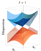
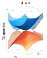
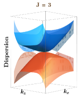
Figure 1: Schematic dispersion of a single tilted node [cf. Eq. (II)] in a (a) Weyl, (b) double-Weyl, and (c) triple-Weyl semimetal, plotted against the $k_{z}k_{x}$-plane. The tilting is taken along the $k_{z}$-direction, along which the dispersion depends linearly on the momentum. The double(triple)-Weyl node shows an anisotropic hybrid dispersion with a quadratic(cubic)-in-momentum dependence along the $k_{x}$-direction. The direction-dependent features are depicted more clearly with the help of the projections of the dispersion along the respective momentum axes.

Anisotropy arising from tilting of the dispersion [56, 57] is often neglected because enters the Hamiltonian with an identity matrix, thus not affecting the eigenspinors and, hence, the topology of the low-energy theory in the vicinity of the band-crossing point. Tilting is generic in the absence of certain discrete symmetries, such as particle-hole and lattice point group symmetries (e.g., the Berry curvature of the Weyl cone does not depend on the tilt parameter). Therefore, tilted dispersion is expected to be present in WSMs/mWSMs in generic situations because of the generic nature of nodal points in 3d [58] (e.g., in a WSM with broken $\mathcal{T}$ [56]), made possible by their topological stability. In the presence of a tilt for one of the momentum directions, which we take to be the $k_{z}$-component in this paper, the LMR has a term with linear-in-$B$ behaviour [59, 60]. Such linear terms may also arise when cubic-in-momentum band-bending terms ($\propto k_{z}^{3}\,\sigma_{z}$) are included in the Hamiltonian [61], which breaks the time-reversal symmetry $\mathcal{T}$. Furthermore, in a PHE set-up, tilting leads to the presence of terms linearly dependent on $B$ in the theoretical expressions of the longitudinal and transverse components of the magnetoelectric conductivity tensor [62, 63, 64, 65]. This can explain the resistivity behaviour in experimental observations [66]. Our aim is to demonstrate how tilt parameters as well as the intrinsic mixed linear-nonlinear dipersion of mWSMs lead to clear signatures in PHE, which are strongly direction-dependent. We show that the $\mathcal{T}$-breaking induced by the tilt of nodes produces linear-in-$B$ corrections, which depend on the direction of the tilt in a PHE set-up.

In this paper, we will consider an experimental set-up when 3d semimetal is subjected to the combined effects of a static uniform external electric field $\mathbf{E}$, applied along the unit vector $\hat{\mathbf{e}}_{E}$, and a uniform external magnetic field $\mathbf{B}$ applied along the unit vector $\hat{\mathbf{e}}_{B}$. If $\hat{\mathbf{e}}_{E}\cdot\hat{\mathbf{e}}_{B}\neq 0$, although the conventional Hall voltage induced from the Lorentz force is zero along $\hat{\mathbf{e}}_{B}$, a node with a nonzero Berry monopole charge (i.e., a nonzero Chern number) gives rise to a voltage difference along this direction. This is the PHE discussed above [22, 28, 67, 29, 36, 30, 68]. The resulting components of the conductivity tensor, which lie in the $\hat{\mathbf{e}}_{E}\,\hat{\mathbf{e}}_{B}$-plane, are commonly known as the longitudinal magnetoconductivity (LMC) and the planar Hall conductivity (PHC). Their behaviour in various experimental set-ups has been extensively investigated in the literature [69, 70, 38, 71, 72, 73, 74, 75, 76, 77, 32]. An untilted WSM is intrinsically isotropic and, hence, it will show the same response irrespective of how we choose to orient the $\hat{\mathbf{e}}_{E}$ and $\hat{\mathbf{e}}_{B}$ unit vectors. However, as soon as we introduce a tilt, it introduces an anisotropy, which should give rise to a direction-dependent response. For the mWSMs, even the untilted cases are anisotropic due to the fact that they feature a hybrid of a linear dispersion along one direction and a quadratic/cubic dispersion in the plane perpendicular to it. Ref. [38] discusses the changes in the zero-temperature PHE response in WSMs, induced by changing the direction of $\mathbf{B}$ with respect to the tilt direction. In another study [73], the authors have derived the response in such PHE set-ups using pseudospin-1 quasiparticles, described by three-band Hamiltonians, which have anisotropic hybrid dispersions analogous to the mWSMs. They did not include tilt in their computations.

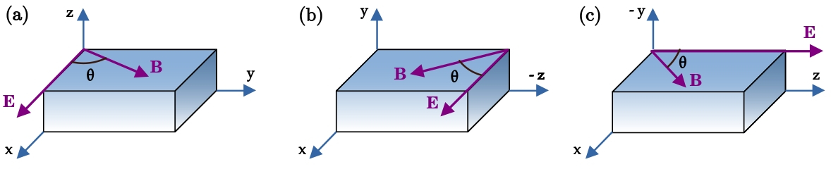
Figure 2: Schematics of the three set-ups that we have used for investigating the planar Hall effect in WSMs/mWSMs, showing the relative orientations of the external homogeneous electric $\mathbf{E}$ and magnetic $\mathbf{B}$ fields, which we label as (a) set-up I, (b) set-up II, and (c) set-up III, respectively. Each type of semimetal has a direction along which the dispersion is linear-in-momentum, which we have chosen to be the $z$-direction, which is also the axis with respect to which the dispersion has a tilt [cf. Fig. 1 and Eq. (II)].

Here we choose a tilt along the $k_{z}$-direction for each case, which maintains an isotropy in the $xy$-plane. The resulting dispersion is shown schematically in Fig. 1. With these considerations in mind, we have three distinct configurations for applying $\mathbf{E}$ and $\mathbf{B}$ in a planar Hall set-up, which are illustrated in Fig. 2. In the first two set-ups, which we label as I and II, $\hat{\mathbf{e}}_{E}$ is set perpendicular to the $k_{z}$-axis, which we have chosen to be the $x$-axis. In set-up I, we orient $\hat{\mathbf{e}}_{B}$ to lie in the $xy$-plane, while in set-up II, we orient $\hat{\mathbf{e}}_{B}$ to lie in the $zx$-plane. In the last set-up, which we denote as set-up III, $\hat{\mathbf{e}}_{E}$ is set parallel to the tilt-axis and $\hat{\mathbf{e}}_{B}$ lies in the $zx$-plane. In each case, $\hat{\mathbf{e}}_{B}$ makes an angle $\theta$ with $\hat{\mathbf{e}}_{A}$, which is not $\pi/2$ in general for observing the PHE. We will employ the semiclassical Boltzmann transport formalism, which works well for small magnetic fields and small cyclotron frequency $\omega_{c}$ such that the Landau quantization can be ignored. The regime of validity is given by $\hbar\,\omega_{c}\ll\mu$, where $\mu$ is the chemical potential/Fermi level.

In the presence of $\mathcal{T}$, the Onsager-Casimir reciprocity relations [78, 79, 80] constrain the $\mathbf{B}$-dependence of the conductivity tensor $\sigma_{pq}$ (where $\{p,q\}$ are the indices denoting the tensor components along the axes of a chosen set of Cartesian coordinates) to be $\sigma_{\tilde{x}\tilde{x}}(\mathbf{B})=\sigma_{\tilde{x}\tilde{x}}(-\mathbf{B})$ and $\sigma_{\tilde{x}\tilde{y}}(\mathbf{B})=\sigma_{\tilde{y}\tilde{x}}(-\mathbf{B})$, with $\tilde{x}$ denoting an axis along $\hat{\mathbf{e}}_{E}$ and $\tilde{y}$ aligned perpendicular to $\tilde{x}$. However, a finite tilt breaks $\mathcal{T}$, thus opening up the possibility of terms containing terms linearly dependent on $B$. An in-depth analysis of the effects of spatial symmetries on PHE can be found in Ref. [81].

The paper is organized as follows: In Sec. II, we introduce the low-energy effective Hamiltonians in the vicinity of a tilted WSM/mWSM node. In Sec. III, we outline the steps to compute the conductivity tensor. Sec. IV is devoted to the demonstrating the explicit expressions of the longitudinal and transverse components of the conductivity tensor and illustrating their behaviour in some relevant parameter regimes. Finally, we conclude with a summary and outlook in Sec. V. In all expressions that follow, we will use the natural units by setting the reduced Planck’s constant ($\hbar$), the speed of light ($c$), and the Boltzmann constant ($k_{B}$) to unity We also show the representative values of the various parameters, appearing in the Hamiltonians and the expressions for the conductivity tensors, using both the SI and the natural units in Table 1.

II Model for a tilted WMS/mWSM node

In the vicinity of a nodal point with chirality $\chi$ and Berry monopole charge of magnitude $J$, the effective continuum Hamiltonian is given by [18, 7, 8]

$$\mathcal{H}_{J}({\mathbf{k}}) =\mathbf{d}({\mathbf{k}})\cdot\bm{\sigma}+\eta\,v_{0}\,k_{z}\,\sigma_{0}\,,\quad\mathbf{d}(\mathbf{k})=\left\{\alpha_{J}\,k_{\perp}^{J}\cos(J\,\phi),\,\alpha_{J}\,k_{\perp}^{J}\sin(J\,\phi),\,\chi\,v_{0}\,k_{z}\right\},$$

$$k_{\perp} =\sqrt{k_{x}^{2}+k_{y}^{2}}\,,\quad\phi=\arctan({\frac{k_{y}}{k_{x}}})\,,\quad\alpha_{J}=\frac{v_{\perp}}{k_{0}^{J-1}}\,,$$ (1)

where $\chi=\pm 1$, $v_{0}$($v_{\perp}$) is the Fermi velocity along the $z$-direction($xy$-plane), $k_{0}$ is a material-dependent parameter with the dimension of momentum, and $\eta$ is the tilt parameter is taken along the $k_{z}$-direction. Henceforth, we will consider the positive-chirality node by setting $\chi=1$. The eigenvalues of the Hamiltonian are given by

$$\mathcal{E}_{\eta,s}({{\mathbf{k}}})=\eta\,v_{0}\,k_{z}-(-1)^{s}\,|\mathbf{d}({\mathbf{k}})|\,,\quad s\in\{1,2\},$$ (2)

where the value $1$($2$) for $s$ represents the upper(lower) band. The Hamiltonian for a WSM node is isotropic in absence of the tilt, which is recovered from $\mathcal{H}_{J}$ by setting $J=1$ and $\alpha_{1}=v_{0}$. Fig. 1 shows the schematic dispersion against the $k_{z}k_{x}$-plane. In this paper, we restrict ourselves to the type-I phases such that $|\eta|<1$, which gives a Fermi point, an electron, or a hole pocket, depending on whether the chemical potential cuts the nodal point, the upper band, or the lower band.

The Berry curvature (BC) associated with the $s^{\rm{th}}$ band is given by [82, 36]

$${\mathbf{\Omega}}_{s}({\mathbf{k}}) =i\,\langle\nabla_{{\mathbf{k}}}\psi_{s}({{\mathbf{k}}})|\,\crossproduct\,|\nabla_{{\mathbf{k}}}\psi_{s}({{\mathbf{k}}})\rangle\Rightarrow\Omega^{a}_{s}({\mathbf{k}})=\frac{-(-1)^{s}\,\,\epsilon^{a}_{\,\,bc}}{4\,|\mathbf{d}({\mathbf{k}})|^{3}}\,\mathbf{d}({\mathbf{k}})\cdot\left[\partial_{k_{b}}\mathbf{d}({\mathbf{k}})\crossproduct\partial_{k_{c}}\mathbf{d}({\mathbf{k}})\right],$$ (3)

where the set of indices $\{a,b,c\}$ takes values from $\{x,y,z\}$ and are used to denote the components of the Cartesian vectors and tensors. The BC arises from the Berry phases generated by $|\psi_{s}(\mathbf{k})\rangle$, where $\{|\psi_{s}(\mathbf{k})\rangle\}$ denotes the set of orthonormal Bloch cell eigenstates for the single-particle Hamiltonian $\mathcal{H}_{J}(\mathbf{k})$. On evaluating the expressions in Eq. (3) using Eq. (II), we get

$${\mathbf{\Omega}}_{s}({{\mathbf{k}}})=\frac{(-1)^{s}\,J\,v_{0}\,\alpha_{J}^{2}\,k_{\perp}^{2J-2}}{2\,\left|\mathbf{d}({\mathbf{k}})\right|^{3}}\left\{k_{x},\,k_{y},\,J\,k_{z}\right\}.$$ (4)

The Bloch velocity vector for the quasiparticles occupying the $s^{\rm th}$ is given by

$${\bm{v}}_{s}({\mathbf{k}})=\nabla_{{\mathbf{k}}}\,\mathcal{E}_{\eta,s}({{\mathbf{k}}})\equiv\nabla_{\mathbf{k}}\,\mathcal{E}_{\chi,s}({\mathbf{k}})=-\frac{(-1)^{s}}{\left|\mathbf{d}({\mathbf{k}})\right|}\left\{J\,\alpha_{J}^{2}\,k_{\perp}^{2J-2}\,k_{x},\,J\,\alpha_{J}^{2}\,k_{\perp}^{2J-2}\,k_{y},\,v_{0}^{2}\,k_{z}\right\}+\Big{\{}0,0,v_{0}\,\eta\Big{\}}.$$ (5)

We find that the BC is independent of the tilt, as expected, while the $z$-component of ${\bm{v}}_{s}(\mathbf{k})$ gets shifted due to the tilt term. In this paper, we will take a positive value of the chemical potential $\mu$ such that it cuts the conduction band with $s=1$. Henceforth, we use the notations $\mathcal{E}_{\eta,1}=\mathcal{E}$, ${\mathbf{\Omega}}_{1}={\mathbf{\Omega}}$, and ${\bm{v}}_{1}={\bm{v}}$, in order to avoid cluttering.

III Magnetoelectric conductivity

We use the semiclassical Boltzmann formalism to find the form of the magnetoelectric conductivity tensor $\sigma_{pq}$ in a generic PHE set-up. We employ a relaxation-time approximation for the collision integral and, furthermore, assume a momentum-independent relaxation time $\tau$, which we treat as a phenomenological constant. We focus on the scenario when the internode scattering amplitude is negligible compared to the intranode scattering amplitude, which suppresses any relaxation towards equal occupation of the two nodes in a conjugate pair, thereby enhancing signatures of the chiral anomaly [22, 23]. Therefore, $\tau$ corresponds solely to the intranode scattering time. The derivation is outlined in detail in Refs. [83, 32]. The final expression for conductivity, contributed by the conduction band at the node with positive chirality, is given by

$$\sigma_{pq}^{\rm tot}=\sigma_{pq}^{\rm AHE}+\sigma_{ab}^{\mathbf{\Gamma}}+\sigma_{pq}\,,\quad\sigma_{pq}^{\rm AHE}=-{e^{2}}\,\int\frac{d^{3}\mathbf{k}}{(2\,\pi)^{3}}\,\epsilon_{pqr}\,\Omega^{r}\,f_{eq}(\mathcal{E})\,,$$

$$\sigma_{pq}=-e^{2}\,\tau\int\frac{d^{3}\mathbf{k}}{(2\,\pi)^{3}}\,\mathcal{D}\left[v_{p}+{e\,B_{p}}\left({\bm{v}}\cdot\mathbf{\Omega}\right)\right]\left[v_{q}+e\,B_{q}\left({\bm{v}}\cdot\mathbf{\Omega}\right)\right]\,\frac{\partial f_{eq}(\mathcal{E})}{\partial\mathcal{E}}\,,$$ (6)

where

$$\mathcal{D}=\left(1+{e}\,{\mathbf{B}}\cdot\mathbf{\Omega}\right)^{-1}$$ (7)

is the phase-space factor which takes into account the the modified density of states in the presence of an external magnetic field, and

$$f_{eq}\big{(}\epsilon\big{)}=\frac{1}{e^{\beta\,\left(\epsilon-\mu\right)}+1}$$ (8)

represents the equilibrium distribution function of the fermionic quasiparticles with $\beta^{-1}=k_{B}\,T$). We have taken the charge of eah quaiparticle to be $-e$, where $e$ is the magnitude of the charge of an electron. The first part, labelled as $\sigma_{ab}^{\chi,\,\rm AHE}$, represents the “intrinsic anomalous” Hall effect [33, 34, 35]. The second part $\sigma_{ab}^{\chi,\,\mathbf{\Gamma}}$ is the Lorentz-force contribution to the conductivity. The last term $\sigma_{ab}^{\chi}$ is the Berry-curvature-related conductivity coefficient. For a momentum-independent $\tau$, $\sigma_{pq}^{\mathbf{\Gamma}}$ is an order of magnitude smaller than the other terms [29] in typical WSMs/mWSM and, hence, we neglect it. Furthermore, we are not interested in $\sigma_{ab}^{\chi,\,\rm AHE}$ because, together with the contribution from the node with opposite chirality, it leads to an overall zero contribution when we sum the conductivity coming from the two nodes.

For the ease of calculations, we decompose $\sigma_{ab}$ into four parts as follows:

$$\sigma_{pq}^{(1)} =\tau\,e^{2}\int\frac{d^{3}{\mathbf{k}}}{(2\,\pi)^{3}}\,\mathcal{D}\,\,v_{p}({\mathbf{k}})\,v_{q}({\mathbf{k}})\,\left[-\frac{\partial f_{eq}(\mathcal{E})}{\partial\mathcal{E}}\right],$$

$$\sigma_{pq}^{(2)} =B_{p}\,B_{q}\,\tau\,e^{4}\int\frac{d^{3}{\mathbf{k}}}{(2\,\pi)^{3}}\,\mathcal{D}\,\left[{\bm{v}}({\mathbf{k}})\cdot{\mathbf{\Omega}}({\mathbf{k}})\right]^{2}\left[-\frac{\partial f_{eq}(\mathcal{E})}{\partial\mathcal{E}}\right],$$

$$\sigma_{pq}^{(3)} ={B_{q}\,\tau\,e^{3}}\int\frac{d^{3}\mathbf{k}}{(2\,\pi)^{3}}\,\mathcal{D}\,v_{p}({\mathbf{k}})\left[{\bm{v}}({\mathbf{k}})\cdot{\mathbf{\Omega}}({\mathbf{k}})\right]\left[-\frac{\partial f_{eq}(\mathcal{E})}{\partial\mathcal{E}}\right],$$

$$\sigma_{pq}^{(4)} ={B_{p}\,\tau\,e^{3}}\int\frac{d^{3}{\mathbf{k}}}{(2\,\pi)^{3}}\,\mathcal{D}\,v_{q}({\mathbf{k}})\left[{\bm{v}}({\mathbf{k}})\cdot{\mathbf{\Omega}}({\mathbf{k}})\right]\left[-\frac{\partial f_{eq}(\mathcal{E})}{\partial\mathcal{E}}\right].$$ (9)

We find that $\sigma_{pq}^{(2)}$, $\sigma_{pq}^{(3)}$, and $\sigma_{pq}^{(4)}$ go to zero if the BC vanishes. We will expand $\mathcal{D}$ in powers of $\mathbf{B}\cdot\mathbf{\Omega}$, restricting to the regime with a weak strength of the magnetic field, and keep terms upto order $\left(\mathbf{B}\cdot\mathbf{\Omega}\right)^{2}$ in the expressions for $\sigma_{pq}$.

Now we outline the details for obtaining the final form of the LMC only for the set-up I, as the others can be derived in a similar way. For this case, we have to set $\hat{\mathbf{e}}_{E}={\mathbf{\hat{x}}}$ and $\hat{\mathbf{e}}_{B}=\cos\theta\,{\mathbf{\hat{x}}}+\sin\theta\,{\mathbf{\hat{y}}}$. Hence, the LMC is given by

$$\sigma_{xx}=\sigma_{xx}^{(1)}+\sigma_{xx}^{(2)}+\sigma_{xx}^{(3)}+\sigma_{xx}^{(4)}\,,$$

where

$$\sigma_{xx}^{(1)} =-\tau\,e^{2}\int\frac{d^{3}\mathbf{k}}{(2\pi)^{3}}\,\mathcal{D}\,v_{x}^{2}({\mathbf{k}})\,\frac{\partial f_{eq}(\mathcal{E})}{\partial\mathcal{E}}\,,\quad\sigma_{xx}^{(2)}=-\tau\,e^{4}\,B_{x}^{2}\int\frac{d^{3}{\mathbf{k}}}{(2\pi)^{3}}\,\mathcal{D}\left[{\bm{v}}({\mathbf{k}})\cdot\mathbf{\Omega}({\mathbf{k}})\right]^{2}\,\frac{\partial f_{eq}(\mathcal{E})}{\partial\mathcal{E}}\,,$$

$$\sigma_{xx}^{(3)} =\sigma_{xx}^{(4)}=-\,\tau\,e^{3}\,B_{x}\int\frac{d^{3}{\mathbf{k}}}{(2\pi)^{3}}\,\mathcal{D}\,v_{x}({\mathbf{k}})\left[{\bm{v}}({\mathbf{k}})\cdot\mathbf{\Omega}({\mathbf{k}})\right]\,\frac{\partial f_{eq}(\mathcal{E})}{\partial\mathcal{E}}\,.$$ (10)

Keeping terms upto $\mathcal{O}\big{(}B^{2}\big{)}$, we obtain

$$\sigma_{xx}^{(1)}=-\frac{\tau\,e^{2}}{(2\pi)^{3}}\,\sum_{j=0}^{2}\int_{0}^{\infty}dk_{\perp}\,\int_{-\infty}^{\infty}\,dk_{z}\,\int_{0}^{2\pi}\,d\phi\,k_{\perp}\,v_{x}^{2}\,\left[-e\,({\mathbf{B}}\cdot{\mathbf{\Omega}})\right]^{j}\frac{\partial f_{eq}(\mathcal{E})}{\partial\mathcal{E}}\,$$ (11)

Changing the integration variables as

$$k_{\perp}=\alpha_{J}^{-1/J}\,\epsilon^{1/J}\left(\sin\gamma\right)^{1/J}\,,\quad k_{z}=\frac{\epsilon\,\cos\gamma}{v_{z}}\,,\quad k_{x}=k_{\perp}\cos\phi\,,\quad k_{y}=k_{\perp}\sin\phi\,,$$ (12)

leads to $\mathcal{E}_{\eta,s}=\epsilon\,\Theta_{s}(\gamma)$, where $\Theta_{s}(\gamma)=s+\eta\cos\gamma$ in general (i.e., irrespective of whether we consider the upper or the lower band). Since we are considering $s=1$ here, we have

$$\sigma_{xx}^{(1)}=\frac{\tau\,e^{2}}{(2\pi)^{3}}\,\frac{J}{v_{0}}\,\sum_{j=0}^{2}\left[\frac{e\,\,v_{0}\,J\,\alpha_{J}^{1/J}}{2}\right]^{j}\int_{0}^{2\,\pi}d\phi\cos^{2}{\phi}\left[B\,\cos{(\theta-\phi)}\right]^{j}\int_{0}^{\pi}d\gamma\left(\sin{\gamma}\right)^{3+j\,\left(2-1/J\right)}\,\mathcal{I}_{1}(j,\gamma)\,,$$ (13)

where

$$\mathcal{I}_{1}(j,\gamma)=\int_{0}^{\infty}d\epsilon\,\epsilon^{2-j\,\left(1+1/J\right)}\frac{\beta e^{\beta\left(\mathcal{E}-\mu\right)}}{\left[1+e^{\beta\,(\mathcal{E}-\mu)}\right]^{2}}\,.$$ (14)

In order to evaluate $\mathcal{I}_{1}(j,\gamma)$, we employ the Sommerfeld expansion

$$\int_{0}^{\infty}d\epsilon\,\epsilon^{n}\,\frac{\beta\,e^{\beta(\mathcal{E}-\mu)}}{\left[1+e^{\beta\,\left(\mathcal{E}-\mu\right)}\right]^{2}}=\frac{1}{\left[\Theta_{1}(\gamma)\right]^{n+1}}\int_{0}^{\infty}d\mathcal{E}\,\mathcal{E}^{n}\frac{\beta\,e^{\beta\,(\mathcal{E}-\mu)}}{(1+e^{\beta\,(\mathcal{E}-\mu)})^{2}}\ =\frac{\Upsilon_{n}(\mu,\beta)}{\left[\Theta_{1}(\gamma)\right]^{n+1}}\,,$$

$$\Upsilon_{n}(\mu,\beta)=\mu^{n}\left[1+\frac{\pi^{2}\,n\,(n-1)}{6\,\beta^{2}\,\mu^{2}}+\frac{7\,\pi^{2}\,n\,(n-3)\,(n-2)\,(n-1)}{360\,\beta^{4}\,\mu^{4}}+\mathcal{O}\Big{(}\left({\beta\,\mu}\right)^{-6}\Big{)}\right],$$ (15)

which is valid in the regime $\beta\mu\gg 1$. Plugging in the above expression, we get

$$\sigma_{xx}^{(1)}=\frac{\tau\,e^{2}}{(2\pi)^{3}}\,\frac{J}{v_{0}}\,\sum_{j=0}^{2}\Upsilon_{2-j\,(1+1/J)}(\mu,\beta)\left[\frac{e\,\,v_{0}\,J\,\alpha_{J}^{1/J}}{2}\right]^{j}\,\int_{0}^{2\pi}d\phi\cos^{2}{\phi}\left[B\,\cos{(\theta-\phi)}\right]^{j}\int_{0}^{\pi}d\gamma\,\frac{(\sin{\gamma})^{3+j\,\left(2-1/J\right)}}{\left[\Theta_{1}(\gamma)\right]^{3-j\,(1+1/J)}}\,.$$ (16)

The last step is to perform the $\gamma$-integral using the identity

$$\int_{0}^{\pi}d\gamma\,\frac{\left(\sin{\gamma}\right)^{m}\left(\cos{\gamma}\right)^{n}}{(1+\eta\cos{\gamma})^{l}}=\int_{-1}^{1}dx\,\frac{\left(1-x^{2}\right)^{\frac{m-1}{2}}x^{n}}{(1+\eta\,x)^{l}}$$

$$=\frac{\sqrt{\pi}\,\,\Gamma(\frac{m+1}{2})}{4}\Bigg{[}2\,\left\{(-1)^{n}+1\right\}\,\Gamma\Big{(}\frac{n+1}{2}\Big{)}\,\,_{3}\tilde{F}_{2}\Big{(}\frac{n+1}{2},\frac{l+1}{2},\frac{l}{2};1/2,\frac{m+n+2}{2};\eta^{2}\Big{)}$$

$$\hskip 78.24507pt+\eta\,l\left\{(-1)^{n}-1\right\}\,\Gamma\Big{(}\frac{n}{2}+1\Big{)}\,_{3}\tilde{F}_{2}\Big{(}\frac{n+2}{2},\frac{l+1}{2},\frac{l+2}{2};3/2,\frac{m+n+3}{2};\eta^{2}\Big{)}\Bigg{]}\,,$$ (17)

where ${}_{n_{1}}\tilde{F}_{n_{2}}\big{(}\{a_{1},\ldots,a_{n_{1}}\};\{b_{1},\ldots,b_{n_{2}}\};X\big{)}$ is a regularized hypergeometric function [84]. Implementing this, we finally get

$$\sigma_{xx}^{(1)} =\sigma_{{\text{Drude}}}+\sigma_{xx}^{{(1,\text{BC})}}\,,$$ (18)

$$\sigma_{{\text{Drude}}} =\,J\,e^{2}\,\tau\,\,\Upsilon_{2}(\mu,\beta)\left[\frac{\delta_{\eta,0}}{6\,\pi^{2}\,v_{0}}+\frac{\delta_{\eta,0}-1}{4\,\pi^{2}\,\eta^{3}\,v_{0}}\left(\frac{\eta}{\eta^{2}-1}+\tanh^{-1}\eta\right)\right],$$ (19)

$$\sigma_{xx}^{{(1,\text{BC})}} =\frac{J^{3}\,e^{4}\,\tau\,B^{2}\,\alpha^{{2}/{J}}\left(3\,\cos^{2}\theta+\sin^{2}\theta\right)\,\Gamma(4-1/J)\,v_{0}}{128\,\pi^{3/2}}\,_{2}\tilde{F}_{1}(1/2-1/J,(J-1)/J;9/2-1/J;\eta^{2})\,\Upsilon_{-{2}/{J}}(\mu,\beta)\,,$$ (20)

where $\sigma_{{\text{Drude}}}$ is independent of the of the magnetic field and is usually referred to as the Drude contribution. The second part $\sigma_{xx}^{{(1,\text{BC})}}$ arises from a nonzero BC. Although here we do not have any linear-in-$B$ term, we will find it in the other set-ups. Proceeding in the way explained above, we obtain the final expressions of $\sigma_{xx}(2)$ , $\sigma_{xx}^{(3)}$, and $\sigma_{xx}^{(4)}$, the steps of which are not very necessary to write down explicitly. In any case, the steps can be found in Ref. [32] and we provide the full final expressions for each set-up in the corresponding subsections of Sec. IV.

Parameter	SI Units	Natural Units
$v_{0}$ from Ref. [85]	$1.5\times 10^{5}$ m s-1	$0.005$
$\tau$ from Ref. [85]	$10^{-13}\,\text{s}$	$151.72$ eV-1
$T$ from Refs. [30, 66]	$0-100\,\text{K}$	$0-8.617\crossproduct 10^{-3}\text{eV}$
$B$ from Ref. [86]	$0.033-0.421\,\text{Tesla}$	$2-25\,\text{eV${}^{2}$}$
$\mu$ from Refs. [73, 60]	$0.1-1$ eV	$0.1-1$ eV

Table 1: We list the parameter regimes which we have used in plotting the components of conductivity tensor. Using the relation $\alpha_{J}={v_{\perp}}/{k_{0}^{J-1}}$, we get $\alpha_{1}=v_{\perp}$, $\alpha_{2}=\frac{v_{\perp}}{k_{0}}$, and $\alpha_{3}=\frac{v_{\perp}}{k_{0}^{2}}=\frac{\alpha_{2}^{2}}{\alpha_{1}}$. In terms of natural units, we need to set $\hbar=c=k_{B}=1$, and $4\,\pi\,\epsilon_{0}=137$. In our plots, we have used $v_{\perp}=v_{0}$ (from the table entry), leading to $\alpha_{2}=3.9\times 10^{-5}$ eV^-1 and $\alpha_{3}=2.298\times 10^{-6}$ eV^-2. For $J=2$ and $J=3$, $v_{\perp}$ has been set equal to $v_{0}$ for the sake of simplicity, while for the isotropic dispersion (modulo the tilt) of $J=1$, we have $v_{\perp}=v_{0}$.

IV Results

In this section, we explicitly write down the expressions of the nonzero components of the magnetoelectric conductivity tensor for the three distinct set-ups shown in Fig. 2. We also illustrate their behaviour by some representative plots and discuss their characteristics.

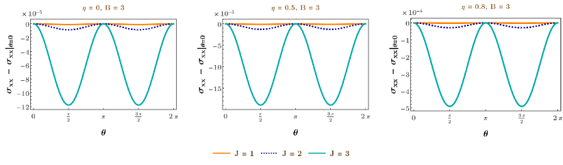
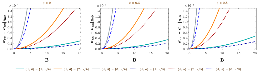
Figure 3: Set-up I: Variation of the LMC (in units of eV²) with (a) the angle $\theta$ and (b) the magnitude ($B$ in units of eV²) of the magnetic field. For all the plots, we have set $v_{0}=0.005$, $\tau=151$ eV^-1, $\mu=0.1$ eV, and $\beta=1160$ eV^-1.

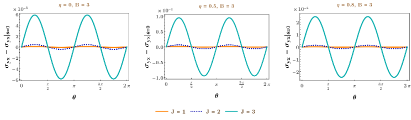
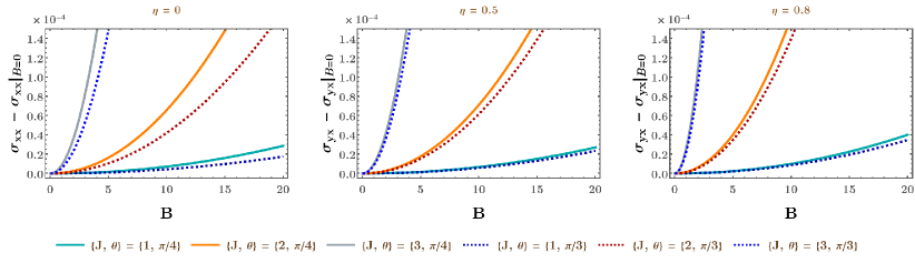
Figure 4: Set-up I: Variation of the PHC (in units of eV²) with (a) the angle $\theta$ and (b) the magnitude ($B$ in units of eV²) of the magnetic field. For all the plots, we have set $v_{0}=0.005$, $\tau=151$ eV^-1, $\mu=0.1$ eV, and $\beta=1160$ eV^-1.

IV.1 Set-up I

In set-up I, as shown in Fig. 2(a), the tilt-axis is perpendicular to the plane made by $\mathbf{E}$ and $\mathbf{B}$. Since here is a rotational symmetry of the dispersion of each semimetallic nodes within the $xy$-plane, therefore the exact direction of $\mathbf{E}$ and $\mathbf{B}$ will not matter. What matters is the angle between $\hat{\mathbf{e}}_{E}$ and $\hat{\mathbf{e}}_{B}$. Hence, without any loss of generality, we choose $\hat{\mathbf{e}}_{E}={\mathbf{\hat{x}}}$ and $\hat{\mathbf{e}}_{B}=\cos\theta\,{\mathbf{\hat{x}}}+\sin\theta\,{\mathbf{\hat{y}}}$.

The full expression for the LMC is given by

$$\sigma_{xx} =\sigma_{xx}^{(1)}+\sigma_{xx}^{(2)}+\sigma_{xx}^{(3)}+\sigma_{xx}^{(4)}\,,$$ (21)

where $\sigma_{xx}^{(1)}$ is already shown in Eq. (18) and

$$\sigma_{xx}^{(2)} =\frac{J^{3}\,e^{4}\,\tau\,\alpha^{2/J}\,B^{2}\cos^{2}\theta\,\,\Gamma(2-1/J)\,v_{0}}{16\,\pi^{3/2}}\,_{2}\tilde{F}_{1}(3/2-1/J,2-1/J;5/2-1/J;\eta^{2})\,\Upsilon_{-2/J}(\mu,\beta)\,,$$

$$\sigma_{xx}^{(3)} =\sigma_{xx}^{(4)}=-\frac{J^{3}\,e^{4}\,\tau\,\alpha^{2/J}\,B^{2}\cos^{2}\theta\,\,\Gamma(3-1/J)\,v_{0}}{32\,\pi^{3/2}}\,_{2}\tilde{F}_{1}(3/2-1/J,(J-1)/J;7/2-1/J;\eta^{2})\,\Upsilon_{-2/J}(\mu,\beta)\,.$$ (22)

From Eq. (19), we find that the Drude part is an even function of $\eta$. The remaining parts, dependent on a nonzero BC, are functions of $\eta^{2}$, thus making them even functions of $\eta$ as well. For this set-up, only even powers of $B$ appear and we do not obtain any part linearly varying with $B$, similar to the untilted cases [30, 42]. Also important to note is that the BC-dependent part is independent of the chirality of the node. This is because the terms in the integrand contributing to a nonzero result involve only even powers of the components of the BC (which is proportional to $\chi$). As a consequence of all these observations, we conclude that if we sum over the contributions from a pair of conjugate nodes, they add up irrespective of whether of the two nodes are tilted in the same or opposite directions. Fig. 3 illustrates the behaviour of the LMC for some representative parameter regimes.

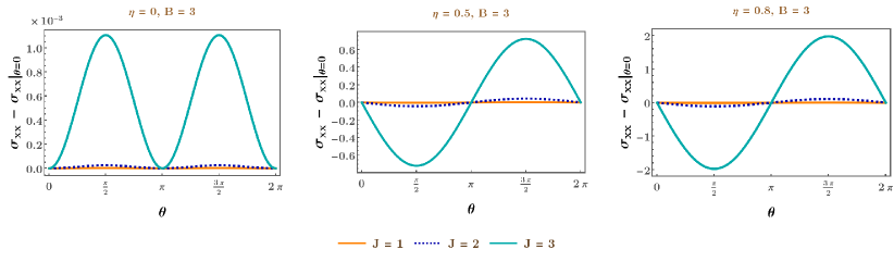
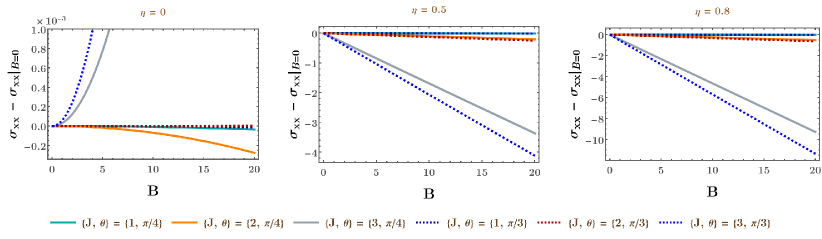
Figure 5: Set-up II: Variation of the LMC (in units of eV²) with (a) the angle $\theta$ and (b) the magnitude ($B$ in units of eV²) of the magnetic field. For all the plots, we have set $v_{0}=0.005$, $\tau=151$ eV^-1, $\mu=0.1$ eV, and $\beta=1160$ eV^-1.

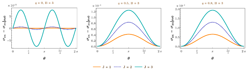
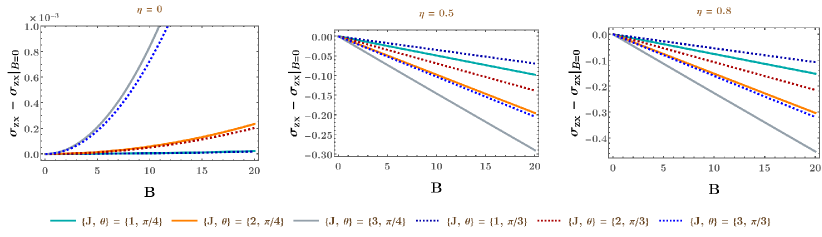
Figure 6: Set-up II: Variation of the PHC (in units of eV²) with (a) the angle $\theta$ and (b) the magnitude ($B$ in units of eV²) of the magnetic field. For all the plots, we have set $v_{0}=0.005$, $\tau=151$ eV^-1, $\mu=0.1$ eV, and $\beta=1160$ eV^-1.

The PHC does not have a Drude part and is entirely caused by a nonzero BC. Explicitly, it takes the form:

$$\sigma_{yx} =\sigma_{yx}^{(1)}+\sigma_{yx}^{(2)}+\sigma_{yx}^{(3)}+\sigma_{yx}^{(4)}\,,\text{ where}$$

$$\sigma_{yx}^{(1)} =\frac{J^{3}\,e^{4}\,\tau\,\alpha^{2/J}\,B^{2}\sin(2\theta)\,\Gamma(4-1/J)\,v_{0}}{32\,\pi^{3/2}}\,_{2}\tilde{F}_{1}(1/2-1/J,(J-1)/J;9/2-1/J;\eta^{2})\,\Upsilon_{-2/J}(\mu,\beta)\,,$$

$$\sigma_{yx}^{(2)} =\frac{J^{3}\,e^{4}\,\tau\,\alpha^{2/J}\,B^{2}\sin(2\theta)\,\Gamma(2-1/J)\,v_{0}}{8\,\pi^{3/2}}\,_{2}\tilde{F}_{1}(3/2-1/J,2-1/J;5/2-1/J;\eta^{2})\,\Upsilon_{-2/J}(\mu,\beta)\,,$$

$$\sigma_{yx}^{(3)} =\sigma_{yx}^{(4)}=-\frac{J^{3}\,e^{4}\,\tau\,\alpha^{2/J}\,B^{2}\sin(2\theta)\,\Gamma(3-1/J)\,v_{0}}{64\,\pi^{3/2}}\,_{2}\tilde{F}_{1}(3/2-1/J,(J-1)/J;7/2-1/J;\eta^{2})\,\Upsilon_{-2/J}(\mu,\beta)\,.$$ (23)

$\sigma_{yx}$ is a function of $\eta^{2}$ and $B^{2}$, and it arises entirely from even powers of the components of the BC (making it independent of the chirality of the node). Hence, analogous to the PHC, it will give the same contribution from each conjugate node, irrespective of the sign of the tilt. However, unlike the LMC, the PHC vanishes when $\theta$ equals zero or $\pi/2$. Fig. 4 demonstrates the characteristics of $\sigma_{yx}$ for some representative parameter regimes.

IV.2 Set-up II

In set-up II, as shown in Fig. 2(b), the tilt-axis is perpendicular to $\mathbf{E}$ but not to $\mathbf{B}$. We choose $\hat{\mathbf{e}}_{E}={\mathbf{\hat{x}}}$ and $\hat{\mathbf{e}}_{B}=\cos\theta\,{\mathbf{\hat{x}}}+\sin\theta\,{\mathbf{\hat{z}}}$.

The full expression for the LMC is given by

$$\sigma_{xx} =\sigma_{\text{Drude}}+\sigma_{xx}^{(1,\text{BC})}+\sigma_{xx}^{(2)}+\sigma_{xx}^{(3)}+\sigma_{xx}^{(4)}\,,$$ (24)

where $\sigma_{\text{Drude}}$ is the same as shown in Eq. (19),

$$\sigma_{xx}^{(1,\text{BC})} =-\frac{\eta\,J^{2}\,e^{3}\,\tau\,(3\,J-2)\,\alpha^{2/J}B\sin\theta\,\Gamma(3-1/J)}{32\,\pi^{3/2}\,v_{0}}\,_{2}\tilde{F}_{1}(2-1/J,5/2-1/J;9/2-1/J;\eta^{2})\,\Upsilon_{2-2/J}(\mu,\beta)$$

$$\quad+\frac{3\,J^{3}\,e^{4}\,\tau\,\alpha^{2/J}\,B^{2}\cos^{2}\theta\,\,\Gamma(4-1/J)\,v_{0}}{128\,\pi^{3/2}}\,_{2}\tilde{F}_{1}(1/2-1/J,(J-1)/J;9/2-1/J;\eta^{2})\,\Upsilon_{-2/J}(\mu,\beta)$$

$$\quad+\frac{J^{5}\,e^{4}\,\tau\,\alpha^{\frac{4}{J}}\,B^{2}\sin^{2}\theta\,\,\Gamma(4-2/J)}{64\,\pi\,v_{0}}\,_{3}\tilde{F}_{2}(3/2,2-2/J,3/2-2/J;1/2,11/2-2/J;\eta^{2})\,\Upsilon_{2-\frac{4}{J}}(\mu,\beta)\,,$$ (25)

$$\sigma_{xx}^{(2)} =\frac{J^{3}\,e^{4}\,\tau\,\alpha^{2/J}\,B^{2}\cos^{2}\theta\,\,\Gamma(2-1/J)\,v_{0}}{16\,\pi^{3/2}}\,_{2}\tilde{F}_{1}(-1/J,-(J+2)/(2J);5/2-1/J;\eta^{2})\,\Upsilon_{-2/J}(\mu,\beta)\,,$$ (26)

and

$$\sigma_{xx}^{(3)} =\sigma_{xx}^{(4)}=-\frac{J^{3}\,e^{4}\,\tau\,\alpha^{2/J}\,B^{2}\cos^{2}\theta\,\,\Gamma(3-1/J)\,v_{0}}{32\,\pi^{3/2}}\,_{2}\tilde{F}_{1}(1/2-1/J,-1/J;7/2-1/J;\eta^{2})\,\Upsilon_{-2/J}(\mu,\beta)\,.$$ (27)

The parts other than the Drude contribution originate from a nonzero BC. In this case, we find that $\sigma_{xx}^{(1,\text{BC})}$ has a part which varies linearly in $\eta$ as well as $B$, that originates from the contribution of a term in the integrand which is proportional to the BC (and, consequently, the chirality $\chi$ of the node). This part, being proportional to $\eta\,\chi$, will cancel out when summed over the two nodes in a conjugate pair, if the tilt-signs are the same. The remaining terms are quadratic in both $\eta$ and $B$, and are independent of the chirality. Hence, these parts add up irrespective of the sign of the tilt. Fig. 5 illustrates the behaviour of the LMC for some representative parameter regimes. In particular, the periodicity of the curves, as functions of $\theta$, changes from $\pi$ to $2\pi$ as soon as a nonzero tilt is introduced. Furthermore, Fig. 5 (b) shows that the linear-in-$B$ parts dominate for a nonzero tilt, with the magnitude increasing with increasing $J$ [because of the factor $J^{2}\,(3\,J-2)$, which monotonically increases with $J$]. Most importantly, the dominant $B$-linear terms lead to a change in the overall sign of the LMC, when measured with respect to the $B=0$ case.

Let us elaborate a bit more on the appearance of the term proportional to $\eta\,B\,\chi$. When the system is subjected to homogeneous external fields, then, in the absence of any other scale in the problem, the Onsager-Casimir reciprocity relation $\sigma_{xx}(\mathbf{B})=\sigma_{xx}(-\mathbf{B})$  [78, 79, 80] forbids any term in the LMC to be linear in $B$, unless the change of sign of $\mathbf{B}$ is compensated by a change of sign in another parameter in the system. The tilt vector, defined by $\mathbf{t}=\eta\,{\mathbf{\hat{z}}}$ in this paper, provides us with such a compensating sign, such that we have now the identity $\sigma_{xx}(\mathbf{B},\mathbf{t})=\sigma_{xx}(-\mathbf{B},-\mathbf{t})$, thus fulfilling the Onsager-Casimir constraints [61]. This allows the linear-in-$B$ to appear in $\sigma_{xx}^{(1,\text{BC})}$, with the corresponding part of the magnetocurrent being proportional to $\left(\mathbf{t}\cdot\mathbf{B}\right)\hat{\mathbf{e}}_{E}$, in agreement with the findings of Ref. [38] for WSMs at $T=0$. Because $\hat{\mathbf{e}}_{E}$ is perpendicular to $\mathbf{t}$ in this set-up, the linear contribution vanishes for $\theta=0$. We note that this term has a nontrivial dependence on the chemical potential and the temperature, via the term $\Upsilon_{2-2/J}(\mu,\beta)$, for $J\neq 1$ (because, of course, $\Upsilon_{0}=1$). The fact that the $\mu$-dependence disappears for $J=1$ is consistent with the WSM studies of Ref. [38].

Analogous to set-up I, the PHC does not have a Drude part and is entirely caused by a nonzero BC. Explicitly, it takes the form:

$$\sigma_{zx}=\sigma_{zx}^{(1)}+\sigma_{zx}^{(2)}+\sigma_{zx}^{(3)}+\sigma_{zx}^{(4)}\,,$$

where

$$\sigma_{zx}^{(1)} =-\frac{J\,e^{3}\,\tau\left[3\,\eta-5\,\eta^{2}-3\left(\eta^{2}-1\right)^{2}\tanh^{-1}\eta\right]B\cos\theta\,v_{0}\left(1-\delta_{\eta,0}\right)}{24\,\pi^{2}\,\eta^{4}}$$

$$\quad+\left[\sqrt{\pi}\,J\,\,_{3}\tilde{F}_{2}(3/2,(J-1)/J,1/2-1/J;1/2,9/2-1/J;\eta^{2})-\eta^{2}\left(J-2\right)\,_{2}\tilde{F}_{1}(3/2-1/J,(J-1)/J;9/2-1/J;\eta^{2})\right]$$

$$\hskip 28.45274pt\times\frac{J^{2}\,e^{4}\,\tau\,\alpha^{2/J}\,B^{2}\sin(2\theta)\,\,\Gamma(3-{1}/{J})\,v_{0}\,\Upsilon_{-2/J}(\mu,\beta)}{64\,\pi^{3/2}}\,,$$ (28)

$$\sigma_{zx}^{(2)} =\frac{J^{3}\,e^{4}\,\tau\,\alpha^{2/J}\,B^{2}\sin(2\theta)\,\Gamma(2-1/J)\,v_{0}}{32\,\pi^{3/2}}\,\,_{2}\tilde{F}_{1}(-1/J,-(J+2)/(2\,J);5/2-1/J;\eta^{2})\,\Upsilon_{-2/J}(\mu,\beta)\,,$$ (29)

$$\sigma_{zx}^{(3)} =-\frac{J^{3}\,e^{4}\,\tau\,\alpha^{2/J}\,B^{2}\sin(2\theta)\,\Gamma(3-1/J)\,v_{0}}{64\,\pi^{3/2}}\,\,_{2}\tilde{F}_{1}(1/2-1/J,-1/J;7/2-1/J;\eta^{2})\,\Upsilon_{-2/J}(\mu,\beta)\,,$$ (30)

and

$$\sigma_{zx}^{(4)} =-\frac{\eta\,J\,e^{3}\,\tau\,B\cos\theta\,v_{0}}{4\,\pi^{2}}$$

$$\qquad-\left[\sqrt{\pi}\,J\,_{3}\tilde{F}_{2}(3/2,1/2-1/J,-1/J;1/2,7/2-1/J;\eta^{2})+2\,\eta^{2}\,_{2}\tilde{F}_{1}(1/2-1/J,(J-1)/{J};7/2-1/J;\eta^{2})\right]$$

$$\hskip 42.67912pt\times\frac{J^{2}\,e^{4}\,\tau\,\alpha^{2/J}\,B^{2}\left[-\sin(2\theta)\right]\Gamma(2-1/J)\,v_{0}\,\Upsilon_{-2/J}(\mu,\beta)}{64\,\pi^{3/2}}\,.$$ (31)

Here too we find the emergence of terms proportional to $\text{sgn}(\eta)\,B\,\chi$ [cf. the first terms in $\sigma_{zx}^{(1)}$ and $\sigma_{zx}^{(4)}$], but without having any dependence on $\mu$ or $\beta$ for any $J$ (unlike the LMC). Moreover, they are directly proportional to $J$ as well. The corresponding part of the magnetocurrent is proportional to $\left(\hat{\mathbf{e}}_{E}\cdot\mathbf{B}\right)\mathbf{t}$, in agreement with the findings of Ref. [38] for WSMs at $T=0$. Therefore, this linear contribution vanishes when $\theta=\pi/2$. Fig. 4 demonstrates the characteristics of the full PHC for some representative parameter regimes, where we find the linear term to be dominating the overall behaviour of the curves for tilted nodes, with the magnitude increasing with increasing values of $J$. A nonzero tilt also changes the periodicity of the curves, as functions of $\theta$, from $\pi$ to $2\pi$, and causes an overall change in the sign of the PHC, when measured with respect to the $B=0$ case.

IV.3 Set-up III

In set-up III, as shown in Fig. 2(c), the tilt-axis is parallel to $\mathbf{E}$, such that $\hat{\mathbf{e}}_{E}={\mathbf{\hat{z}}}$, and $\hat{\mathbf{e}}_{B}=\cos\theta\,{\mathbf{\hat{z}}}+\sin\theta\,{\mathbf{\hat{x}}}$.

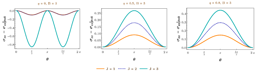
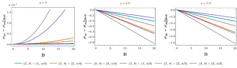
Figure 7: Set-up III: Variation of the LMC (in units of eV²) with (a) the angle $\theta$ and (b) the magnitude ($B$ in units of eV²) of the magnetic field. For all the plots, we have set $v_{0}=0.005$, $\tau=151$ eV^-1, $\mu=0.1$ eV, and $\beta=1160$ eV^-1.

The full expression for the LMC is given by

$$\sigma_{zz} =\tilde{\sigma}_{\text{Drude}}+\sigma_{zz}^{(1,\text{BC})}+\sigma_{zz}^{(2)}+\sigma_{zz}^{(3)}+\sigma_{zz}^{(4)}\,,$$ (32)

where

$$\tilde{\sigma}^{\text{Drude}} =\frac{e^{2}\,\tau\,v_{0}\Upsilon_{2/J}(\mu,\beta)}{8\,\pi^{3/2}\,\alpha^{2/J}\,\Gamma(3/2+1/J)}\left[\Gamma(1+1/J)\,\delta_{\eta,0}+\frac{J+2-2\,\,_{2}F_{1}(1/2,1;3/2+1/J;\eta^{2})}{\left(1-\eta^{2}\right)^{1/J}\,J^{2}}\,\Gamma(1/J)\,(1-\delta_{\eta,0})\right],$$ (33)

$$\sigma_{zz}^{(1,\text{BC})}$$

$$=-\frac{J\,e^{3}\,\tau\,B\cos\theta\,v_{0}\left[3\left(\eta^{2}-1\right)^{2}\tanh^{-1}\eta-3\,\eta^{5}+5\,\eta^{3}-3\,\eta\right]\left(1-\delta_{\eta,0}\right)}{12\,\pi^{2}\,\eta^{4}}$$

$$\quad+\frac{J\,e^{4}\,\tau\,B^{2}\cos^{2}\theta\,v_{0}^{3}\left(7\,\eta^{2}+1\right)\Upsilon_{-2}(\mu,\beta)}{120\,\pi^{2}}$$

$$\quad+\Bigg{[}2\,\eta^{2}J\,_{3}\tilde{F}_{2}(3/2,(J-1)/{J},1/2-1/J;1/2,7/2-1/J;\eta^{2})+3\,J\,_{3}\tilde{F}_{2}(5/2,(J-1)/{J},1/2-1/J;1/2,9/2-1/J;\eta^{2})$$

$$\hskip 28.45274pt-3\,\eta^{2}\left(J-2\right)\,\,_{3}\tilde{F}_{2}\left(5/2,(J-1)/{J},3/2-1/J;3/2,9/2-1/J;\eta^{2}\right)\Bigg{]}\frac{J^{2}\,e^{4}\,\tau\,\alpha^{2/J}\,B^{2}\cos^{2}\theta\,\Gamma(2-1/J)\,v_{0}\,\Upsilon_{-2/J}(\mu,\beta)}{32\,\pi}\,,$$ (34)

$$\sigma_{zz}^{(2)} =\frac{J^{3}e^{4}\tau\alpha^{2/J}\,B^{2}\cos^{2}\theta\,\,\Gamma(2-1/J)\,v_{0}\,\Upsilon_{-2/J}(\mu,\beta)}{16\,\pi^{3/2}}\,_{2}\tilde{F}_{1}\big{(}-1/J,-(J+2)/(2J);5/2-1/J;\eta^{2}\big{)}\,,$$ (35)

$$\sigma_{zz}^{(3)} =\sigma_{zz}^{(4)}=-\frac{\eta\,J\,e^{3}\,\tau\,B\cos\theta\,v_{0}}{4\,\pi^{2}}$$

$$\hskip 42.67912pt-\Bigg{[}\sqrt{\pi}\,J\,\,_{3}\tilde{F}_{2}-(3/2,1/2-1/J,-1/J;1/2,7/2-1/J;\eta^{2})+2\,\eta^{2}\,_{2}\tilde{F}_{1}(1/2-1/J,(J-1)/{J};7/2-1/J;\eta^{2})\Bigg{]}$$

$$\hskip 62.59596pt\times\frac{J^{2}\,e^{4}\,\tau\,\alpha^{2/J}\,B^{2}\cos^{2}\theta\,\Gamma(2-1/J)\,v_{0}\,\Upsilon_{-2/J}(\mu,\beta)}{32\,\pi^{3/2}}\,.$$ (36)

We find that there is a $B$-independent Drude part, viz., $\tilde{\sigma}^{\text{Drude}}$, whose form is different from Eq. (19). However, similar to $\sigma^{\text{Drude}}$, $\tilde{\sigma}^{\text{Drude}}$ is an even function of $\eta$ (independent of $\chi$) and, hence, independent of the sign of the tilt. Analogous to the LMC in set-up II, we find that $\sigma_{zz}^{(1,\text{BC})}$ contains a linear-in-$B$ term, whose behaviour goes as $\propto\text{sgn}(\eta)\,\chi\,B\,J$. In addition, there is another linear-in-$B$ term coming from $\sigma_{zz}^{(3)}$ and $\sigma_{zz}^{(3)}$ with the dependence $\propto\eta\,B\,\chi\,J$. None of these $B$-linear terms has any $\mu$- or $T$-dependence and, while summing over the conjugate nodes of opposite chiralities, the net result will be nonzero only for tilting in opposite directions. The part of the electric current arising from them is proportional to $\left(\mathbf{t}\cdot\mathbf{B}\right)\hat{\mathbf{e}}_{E}$, and the identity $\sigma_{zz}(\mathbf{B},\mathbf{t})=\sigma_{zz}(-\mathbf{B},-\mathbf{t})$ makes it possible to satisfy the Onsager-Casimir reciprocity relations. The remaining terms of $\sigma_{zz}$ are quadratic in $B$, contain even powers of $\eta$, and are independent of the chirality of the node. All the non-Drude terms vanish when $\theta=\pi/2$ and have an overall $2\pi$($\pi$)-periodicity in $\theta$ for nonzero(zero) $\eta$. All these are accompanied by an overall change in sign of the LMC, when measured with respect to the $B=0$ case. The typical characteristics of the LMC are captured in Fig. 7 via some representative parameter regimes.

As for the PHC, we have the simple relation

$$\sigma_{xz}(\theta)\big{|}_{\text{set-up III}}=\sigma_{zx}(\pi/2-\theta)\big{|}_{\text{set-up II}}\,.$$ (37)

Hence, we get a linear term similar to set-up II. The only difference is that here the magnetocurrent, arising from the $B$-linear term, is proportional to $\left(\hat{\mathbf{e}}_{E}\cdot\mathbf{t}\right)\mathbf{B}$.

V Summary and outlook

In this paper, we have delved into the characterization of the magnetoelectric conductivity tensors in the context of planar Hall set-ups built with tilted WSMs and mWSMs, considering various relative orientations of the electromagnetic fields and the direction of the tilt. One instance of the importance of our studies can be motivated as follows. We know that the response in PHE is not solely generated by the chiral anomaly and nonzero BC in the nodal-point semimetals. In fact, it can also have nontopological origins from magnetic order, spin-orbital coupling, and trivial in-plane orbital magnetoresistance [87]. The PHE in nonmagnetic WSMs/mWSMs is dominated by the BC curvature and chiral anomaly contributions only in materials with relatively small orbital magnetoresistance [88]. However, in magnetic WSMs/mWSMs, the response is dominated by the part originating from the Berry phase because the anisotropic magnetic resistance (caused by different in-plane and out-of-plane spin scatterings) induced in ferromagnetism is very small in comparison. The topological and nontopological origins of the PHE, discussed above, cannot always be clearly distinguished in experiments, because the experimentally observed quadratic-in-$B$ magnetoconductance arise via both mechanisms. To remedy the situation, we can use the fact that the Berry curvature gives rise to a linear-in-$B$ term in magnetoconductance if the node is tilted. In fact, our results show that this term dominates in suitable parameter regimes, and increases in magnitude as the magnitude of the monopole charge $J$ increases. Most importantly, the dominant $B$-linear terms lead to a change in sign of the magnetoconductance, when measured with respect to the $B=0$ case.

We would like to point out that we have not considered the OMM in order to make it possible to obtain closed-form expressions from the integrals and to identify the features (e.g., emergence of the linear-in-$\mathbf{B}$ dependence) originating solely from the effects of tilt. This is justified by the fact that the OMM, in the limit of negligible internode scatterings, is not expected to change the qualitative results, and has been neglected in the earlier studies as well [29, 60, 62, 38, 74]. However, in future we will determine how a combination of OMM and significant internode scatterings modify the response, as indicated in Ref. [27]. In order to capture the correct physics, we must go beyond the relaxation-time approximation [27].

In the future, it will be worthwhile to study the influence of a strong quantizing magnetic field, when Landau level formation cannot be ignored [89, 75, 41, 42]. The behaviour of the magnetoconductivity in the presence of disorder as well as many-body interactions [90, 51, 91, 92, 93, 94, 95] will take us into the regime where interactions cannot be ignored. Another possible direction is to investigate the response resulting from an additional time-periodic drive [53, 54, 68] applied on the system (e.g., by shining a beam of circularly polarized light).

References

- Armitage et al. [2018] N. P. Armitage, E. J. Mele, and A. Vishwanath, Weyl and Dirac semimetals in three-dimensional solids, Rev. Mod. Phys. 90, 015001 (2018).
- Burkov and Balents [2011] A. A. Burkov and L. Balents, Weyl semimetal in a topological insulator multilayer, Phys. Rev. Lett. 107, 127205 (2011).
- Yan and Felser [2017] B. Yan and C. Felser, Topological materials: Weyl semimetals, Annual Rev. of Condensed Matter Phys. 8, 337 (2017).
- Adler [1969] S. L. Adler, Axial-vector vertex in spinor electrodynamics, Phys. Rev. 177, 2426 (1969).
- Bell and Jackiw [1969] J. S. Bell and R. Jackiw, A PCAC puzzle: in the model, Nuovo Cim. A 60, 47 (1969).
- Nielsen and Ninomiya [1983] H. Nielsen and M. Ninomiya, The Adler-Bell-Jackiw anomaly and Weyl fermions in a crystal, Physics Letters B 130, 389 (1983).
- Bradlyn et al. [2016] B. Bradlyn, J. Cano, Z. Wang, M. G. Vergniory, C. Felser, R. J. Cava, and B. A. Bernevig, Beyond Dirac and Weyl fermions: Unconventional quasiparticles in conventional crystals, Science 353 (2016).
- Fang et al. [2012] C. Fang, M. J. Gilbert, X. Dai, and B. A. Bernevig, Multi-Weyl topological semimetals stabilized by point group symmetry, Phys. Rev. Lett. 108, 266802 (2012).
- Dantas et al. [2018] R. Dantas, F. Pena-Benitez, B. Roy, and P. Surówka, Magnetotransport in multi-Weyl semimetals: A kinetic theory approach, Journal of High Energy Phys. 2018, 1 (2018).
- Nielsen and Ninomiya [1981] H. Nielsen and M. Ninomiya, A no-go theorem for regularizing chiral fermions, Phys. Lett. B 105, 219 (1981).
- Huang et al. [2015] X. Huang, L. Zhao, Y. Long, P. Wang, D. Chen, Z. Yang, H. Liang, M. Xue, H. Weng, Z. Fang, X. Dai, and G. Chen, Observation of the chiral-anomaly-induced negative magnetoresistance in 3d Weyl semimetal TaAs, Phys. Rev. X 5, 031023 (2015).
- Lv et al. [2015] B. Q. Lv, H. M. Weng, B. B. Fu, X. P. Wang, H. Miao, J. Ma, P. Richard, X. C. Huang, L. X. Zhao, G. F. Chen, Z. Fang, X. Dai, T. Qian, and H. Ding, Experimental Discovery of Weyl Semimetal TaAs, Phys. Rev. X 5, 031013 (2015).
- Xu et al. [2015] S.-Y. Xu, I. Belopolski, N. Alidoust, M. Neupane, G. Bian, C. Zhang, R. Sankar, G. Chang, Z. Yuan, C.-C. Lee, S.-M. Huang, H. Zheng, J. Ma, D. S. Sanchez, B. Wang, A. Bansil, F. Chou, P. P. Shibayev, H. Lin, S. Jia, and M. Z. Hasan, Discovery of a Weyl fermion semimetal and topological Fermi arcs, Science 349, 613 (2015).
- Ruan et al. [2016] J. Ruan, S.-K. Jian, H. Yao, H. Zhang, S.-C. Zhang, and D. Xing, Symmetry-protected ideal Weyl semimetal in HgTe-class materials, Nature Communications 7, 11136 (2016).
- Xu et al. [2011] G. Xu, H. Weng, Z. Wang, X. Dai, and Z. Fang, Chern semimetal and the quantized anomalous Hall effect in HgCr2Se4, Phys. Rev. Lett. 107, 186806 (2011).
- Huang et al. [2016] S.-M. Huang, S.-Y. Xu, I. Belopolski, C.-C. Lee, G. Chang, T.-R. Chang, B. Wang, N. Alidoust, G. Bian, M. Neupane, D. Sanchez, H. Zheng, H.-T. Jeng, A. Bansil, T. Neupert, H. Lin, and M. Z. Hasan, New type of Weyl semimetal with quadratic double weyl fermions, Proceedings of the National Academy of Sciences 113, 1180 (2016).
- Singh et al. [2018] B. Singh, G. Chang, T.-R. Chang, S.-M. Huang, C. Su, M.-C. Lin, H. Lin, and A. Bansil, Tunable double-Weyl fermion semimetal state in the SrSi2 materials class, Scientific Reports 8, 10540 (2018).
- Liu and Zunger [2017] Q. Liu and A. Zunger, Predicted realization of cubic Dirac fermion in quasi-one-dimensional transition-metal monochalcogenides, Phys. Rev. X 7, 021019 (2017).
- Huang et al. [2017] Z.-M. Huang, J. Zhou, and S.-Q. Shen, Topological responses from chiral anomaly in multi-Weyl semimetals, Phys. Rev. B 96, 085201 (2017).
- Goswami et al. [2015] P. Goswami, J. H. Pixley, and S. Das Sarma, Axial anomaly and longitudinal magnetoresistance of a generic three-dimensional metal, Phys. Rev. B 92, 075205 (2015).
- Lv et al. [2021] B. Q. Lv, T. Qian, and H. Ding, Experimental perspective on three-dimensional topological semimetals, Rev. Mod. Phys. 93, 025002 (2021).
- Son and Spivak [2013] D. T. Son and B. Z. Spivak, Chiral anomaly and classical negative magnetoresistance of Weyl metals, Phys. Rev. B 88, 104412 (2013).
- Kim et al. [2014] K.-S. Kim, H.-J. Kim, and M. Sasaki, Boltzmann equation approach to anomalous transport in a Weyl metal, Phys. Rev. B 89, 195137 (2014).
- Moghaddam et al. [2022] A. G. Moghaddam, K. Geishendorf, R. Schlitz, J. I. Facio, P. Vir, C. Shekhar, C. Felser, K. Nielsch, S. T. Goennenwein, J. van den Brink, et al., Observation of an unexpected negative magnetoresistance in magnetic Weyl semimetal Co3Sn2S2, Materials Today Phys. 29, 100896 (2022).
- Xiao et al. [2010] D. Xiao, M.-C. Chang, and Q. Niu, Berry phase effects on electronic properties, Rev. Mod. Phys. 82, 1959 (2010).
- Sundaram and Niu [1999] G. Sundaram and Q. Niu, Wave-packet dynamics in slowly perturbed crystals: Gradient corrections and Berry-phase effects, Phys. Rev. B 59, 14915 (1999).
- Knoll et al. [2020] A. Knoll, C. Timm, and T. Meng, Negative longitudinal magnetoconductance at weak fields in Weyl semimetals, Phys. Rev. B 101, 201402 (2020).
- Burkov [2017] A. A. Burkov, Giant planar Hall effect in topological metals, Phys. Rev. B 96, 041110 (2017).
- Nandy et al. [2017] S. Nandy, G. Sharma, A. Taraphder, and S. Tewari, Chiral anomaly as the origin of the planar Hall effect in Weyl semimetals, Phys. Rev. Lett. 119, 176804 (2017).
- Nag and Nandy [2020] T. Nag and S. Nandy, Magneto-transport phenomena of type-I multi-Weyl semimetals in co-planar setups, Journal of Phys.: Condensed Matter 33, 075504 (2020).
- Medel Onofre and Martín-Ruiz [2023] L. Medel Onofre and A. Martín-Ruiz, Planar Hall effect in Weyl semimetals induced by pseudoelectromagnetic fields, Phys. Rev. B 108, 155132 (2023).
- Ghosh and Mandal [2024] R. Ghosh and I. Mandal, Electric and thermoelectric response for Weyl and multi-Weyl semimetals in planar Hall configurations including the effects of strain, Physica E: Low-dimensional Systems and Nanostructures 159, 115914 (2024).
- Haldane [2004] F. D. M. Haldane, Berry Curvature on the Fermi Surface: Anomalous Hall Effect as a Topological Fermi-Liquid Property, Phys. Rev. Lett. 93, 206602 (2004).
- Goswami and Tewari [2013] P. Goswami and S. Tewari, Axionic field theory of -dimensional Weyl semimetals, Phys. Rev. B 88, 245107 (2013).
- Burkov [2014] A. A. Burkov, Anomalous Hall Effect in Weyl Metals, Phys. Rev. Lett. 113, 187202 (2014).
- Nandy et al. [2018] S. Nandy, A. Taraphder, and S. Tewari, Berry phase theory of planar Hall effect in topological insulators, Scientific Reports 8, 14983 (2018).
- Nandy et al. [2019] S. Nandy, A. Taraphder, and S. Tewari, Planar thermal Hall effect in Weyl semimetals, Phys. Rev. B 100, 115139 (2019).
- Das and Agarwal [2019] K. Das and A. Agarwal, Linear magnetochiral transport in tilted type-I and type-II Weyl semimetals, Phys. Rev. B 99, 085405 (2019).
- Yadav et al. [2022] S. Yadav, S. Fazzini, and I. Mandal, Magneto-transport signatures in periodically-driven Weyl and multi-Weyl semimetals, Physica E: Low-dimensional Systems and Nanostructures 144, 115444 (2022).
- Gusynin et al. [2006] V. Gusynin, S. Sharapov, and J. Carbotte, Magneto-optical conductivity in graphene, Journal of Phys.: Condensed Matter 19, 026222 (2006).
- Stålhammar et al. [2020] M. Stålhammar, J. Larana-Aragon, J. Knolle, and E. J. Bergholtz, Magneto-optical conductivity in generic Weyl semimetals, Phys. Rev. B 102, 235134 (2020).
- Yadav et al. [2023] S. Yadav, S. Sekh, and I. Mandal, Magneto-optical conductivity in the type-I and type-II phases of Weyl/multi-Weyl semimetals, Physica B: Condensed Matter 656, 414765 (2023).
- Papaj and Fu [2019] M. Papaj and L. Fu, Magnus Hall effect, Phys. Rev. Lett. 123, 216802 (2019).
- Mandal et al. [2020] D. Mandal, K. Das, and A. Agarwal, Magnus Nernst and thermal Hall effect, Phys. Rev. B 102, 205414 (2020).
- Sekh, Sajid and Mandal, Ipsita [2022] Sekh, Sajid and Mandal, Ipsita, Magnus Hall effect in three-dimensional topological semimetals, Eur. Phys. J. Plus 137, 736 (2022).
- Sekh and Mandal [2022] S. Sekh and I. Mandal, Circular dichroism as a probe for topology in three-dimensional semimetals, Phys. Rev. B 105, 235403 (2022).
- Mandal [2023a] I. Mandal, Signatures of two- and three-dimensional semimetals from circular dichroism, arXiv e-prints (2023a), arXiv:2302.01829 [cond-mat.mes-hall] .
- Moore [2018] J. E. Moore, Optical properties of Weyl semimetals, National Science Rev. 6, 206 (2018).
- Guo et al. [2023] C. Guo, V. S. Asadchy, B. Zhao, and S. Fan, Light control with Weyl semimetals, eLight 3, 2 (2023).
- Avdoshkin et al. [2020] A. Avdoshkin, V. Kozii, and J. E. Moore, Interactions remove the quantization of the chiral photocurrent at Weyl points, Phys. Rev. Lett. 124, 196603 (2020).
- Mandal [2020] I. Mandal, Effect of interactions on the quantization of the chiral photocurrent for double-Weyl semimetals, Symmetry 12 (2020).
- Mandal and Sen [2021] I. Mandal and A. Sen, Tunneling of multi-Weyl semimetals through a potential barrier under the influence of magnetic fields, Phys. Lett. A 399, 127293 (2021).
- Bera and Mandal [2021] S. Bera and I. Mandal, Floquet scattering of quadratic band-touching semimetals through a time-periodic potential well, Journal of Phys. Condensed Matter 33, 295502 (2021).
- Bera et al. [2023] S. Bera, S. Sekh, and I. Mandal, Floquet transmission in Weyl/multi-Weyl and nodal-line semimetals through a time-periodic potential well, Ann. Phys. (Berlin) 535, 2200460 (2023).
- Mandal [2023b] I. Mandal, Transmission and conductance across junctions of isotropic and anisotropic three-dimensional semimetals, European Physical Journal Plus 138, 1039 (2023b).
- Trescher et al. [2015] M. Trescher, B. Sbierski, P. W. Brouwer, and E. J. Bergholtz, Quantum transport in dirac materials: Signatures of tilted and anisotropic dirac and weyl cones, Phys. Rev. B 91, 115135 (2015).
- Trescher et al. [2017] M. Trescher, B. Sbierski, P. W. Brouwer, and E. J. Bergholtz, Tilted disordered Weyl semimetals, Phys. Rev. B 95, 045139 (2017).
- Herring [1937] C. Herring, Accidental degeneracy in the energy bands of crystals, Phys. Rev. 52, 365 (1937).
- Zyuzin [2017] V. A. Zyuzin, Magnetotransport of Weyl semimetals due to the chiral anomaly, Phys. Rev. B 95, 245128 (2017).
- Sharma et al. [2017] G. Sharma, P. Goswami, and S. Tewari, Chiral anomaly and longitudinal magnetotransport in type-II Weyl semimetals, Phys. Rev. B 96, 045112 (2017).
- Cortijo [2016] A. Cortijo, Linear magnetochiral effect in Weyl semimetals, Phys. Rev. B 94, 241105 (2016).
- Ma et al. [2019] D. Ma, H. Jiang, H. Liu, and X. C. Xie, Planar Hall effect in tilted Weyl semimetals, Phys. Rev. B 99, 115121 (2019).
- Kundu et al. [2020] A. Kundu, Z. B. Siu, H. Yang, and M. B. Jalil, Magnetotransport of Weyl semimetals with tilted Dirac cones, New Journal of Phys. 22, 083081 (2020).
- Könye and Ogata [2021] V. Könye and M. Ogata, Microscopic theory of magnetoconductivity at low magnetic fields in terms of Berry curvature and orbital magnetic moment, Phys. Rev. Res. 3, 033076 (2021).
- Shao and Yan [2022] J. Shao and L. Yan, In-plane magnetotransport phenomena in tilted Weyl semimetals, Journal of Phys.: Condensed Matter 51, 025401 (2022).
- Li et al. [2018] P. Li, C. H. Zhang, J. W. Zhang, Y. Wen, and X. X. Zhang, Giant planar Hall effect in the Dirac semimetal ZrTe5, Phys. Rev. B 98, 121108 (2018).
- Li et al. [2017] Y. Li, Z. Wang, P. Li, X. Yang, Z. Shen, F. Sheng, X. Li, Y. Lu, Y. Zheng, and Z.-A. Xu, Negative magnetoresistance in Weyl semimetals NbAs and NbP: Intrinsic chiral anomaly and extrinsic effects, Frontiers of Phys. 12, 127205 (2017).
- Yadav et al. [2022] S. Yadav, S. Fazzini, and I. Mandal, Magneto-transport signatures in periodically-driven Weyl and multi-Weyl semimetals, Physica E Low-Dimensional Systems and Nanostructures 144, 115444 (2022).
- Zhang et al. [2016] S.-B. Zhang, H.-Z. Lu, and S.-Q. Shen, Linear magnetoconductivity in an intrinsic topological Weyl semimetal, New Journal of Phys. 18, 053039 (2016).
- Chen and Fiete [2016] Q. Chen and G. A. Fiete, Thermoelectric transport in double-Weyl semimetals, Phys. Rev. B 93, 155125 (2016).
- Das and Agarwal [2020] K. Das and A. Agarwal, Thermal and gravitational chiral anomaly induced magneto-transport in Weyl semimetals, Phys. Rev. Res. 2, 013088 (2020).
- Das et al. [2022] S. Das, K. Das, and A. Agarwal, Nonlinear magnetoconductivity in Weyl and multi-Weyl semimetals in quantizing magnetic field, Phys. Rev. B 105, 235408 (2022).
- Pal et al. [2022a] O. Pal, B. Dey, and T. K. Ghosh, Berry curvature induced magnetotransport in 3D noncentrosymmetric metals, Journal of Phys.: Condensed Matter 34, 025702 (2022a).
- Pal et al. [2022b] O. Pal, B. Dey, and T. K. Ghosh, Berry curvature induced anisotropic magnetotransport in a quadratic triple-component fermionic system, Journal of Phys.: Condensed Matter 34, 155702 (2022b).
- Fu and Wang [2022] L. X. Fu and C. M. Wang, Thermoelectric transport of multi-Weyl semimetals in the quantum limit, Phys. Rev. B 105, 035201 (2022).
- Araki [2020] Y. Araki, Magnetic Textures and Dynamics in Magnetic Weyl Semimetals, Annalen der Physik 532, 1900287 (2020).
- [77] Y. P. Mizuta and F. Ishii, Contribution of Berry curvature to thermoelectric effects, in Proceedings of the International Conference on Strongly Correlated Electron Systems (SCES2013).
- Onsager [1931] L. Onsager, Reciprocal Relations in Irreversible Processes. I., Phys. Rev. 37, 405 (1931).
- Casimir [1945] H. B. G. Casimir, On Onsager’s principle of microscopic reversibility, Rev. Mod. Phys. 17, 343 (1945).
- Jacquod et al. [2012] P. Jacquod, R. S. Whitney, J. Meair, and M. Büttiker, Onsager relations in coupled electric, thermoelectric, and spin transport: The tenfold way, Phys. Rev. B 86, 155118 (2012).
- Wei et al. [2023] Y.-W. Wei, J. Feng, and H. Weng, Spatial symmetry modulation of planar Hall effect in Weyl semimetals, Phys. Rev. B 107, 075131 (2023).
- Xiao et al. [2007] D. Xiao, W. Yao, and Q. Niu, Valley-contrasting phys. in graphene: Magnetic moment and topological transport, Phys. Rev. Lett. 99, 236809 (2007).
- Mandal and Saha [2023] I. Mandal and K. Saha, Thermoelectric response in nodal-point semimetals, arXiv e-prints (2023), arXiv:2309.10763 [cond-mat.mes-hall] .
- Weisstein [ Inc] E. W. Weisstein, Regularized hypergeometric function, From MathWorld–A Wolfram Web Resource (Wolfram Research, Inc.).
- Watzman et al. [2018] S. J. Watzman, T. M. McCormick, C. Shekhar, S. C. Wu, Y. Sun, A. Prakash, C. Felser, N. Trivedi, and J. P. Heremans, Dirac dispersion generates unusually large Nernst effect in Weyl semimetals, Phys. Rev. B 97, 161404 (2018).
- Ghosh et al. [2020] S. Ghosh, D. Sinha, S. Nandy, and A. Taraphder, Chirality-dependent planar Hall effect in inhomogeneous Weyl semimetals, Phys. Rev. B 102, 121105 (2020).
- Liu et al. [2019] Q. Liu, F. Fei, B. Chen, X. Bo, B. Wei, S. Zhang, M. Zhang, F. Xie, M. Naveed, X. Wan, F. Song, and B. Wang, Nontopological origin of the planar Hall effect in the type-II Dirac semimetal , Phys. Rev. B 99, 155119 (2019).
- Kumar et al. [2018] N. Kumar, S. N. Guin, C. Felser, and C. Shekhar, Planar Hall effect in the Weyl semimetal GdPtBi, Phys. Rev. B 98, 041103 (2018).
- Mandal and Saha [2020] I. Mandal and K. Saha, Thermopower in an anisotropic two-dimensional Weyl semimetal, Phys. Rev. B 101, 045101 (2020).
- Mandal and Gemsheim [2019] I. Mandal and S. Gemsheim, Emergence of topological Mott insulators in proximity of quadratic band touching points, Condensed Matter Phys. 22, 13701 (2019).
- Mandal [2021] I. Mandal, Robust marginal Fermi liquid in birefringent semimetals, Phys. Lett. A 418, 127707 (2021).
- Mandal and Ziegler [2021] I. Mandal and K. Ziegler, Robust quantum transport at particle-hole symmetry, EPL (EuroPhys. Lett.) 135, 17001 (2021).
- Nandkishore and Parameswaran [2017] R. M. Nandkishore and S. A. Parameswaran, Disorder-driven destruction of a non-Fermi liquid semimetal studied by renormalization group analysis, Phys. Rev. B 95, 205106 (2017).
- Mandal and Nandkishore [2018] I. Mandal and R. M. Nandkishore, Interplay of Coulomb interactions and disorder in three-dimensional quadratic band crossings without time-reversal symmetry and with unequal masses for conduction and valence bands, Phys. Rev. B 97, 125121 (2018).
- Mandal [2018] I. Mandal, Fate of superconductivity in three-dimensional disordered Luttinger semimetals, Annals of Phys. 392, 179 (2018).