Bridging Associative Memory and Probabilistic Modeling

Abstract

Associative memory and probabilistic modeling are two fundamental topics in artificial intelligence. The first studies recurrent neural networks designed to denoise, complete and retrieve data, whereas the second studies learning and sampling from probability distributions. Based on the observation that associative memory’s energy functions can be seen as probabilistic modeling’s negative log likelihoods, we build a bridge between the two that enables useful flow of ideas in both directions. We showcase four examples: First, we propose new energy-based models that flexibly adapt their energy functions to new in-context datasets, an approach we term in-context learning of energy functions. Second, we propose two new associative memory models: one that dynamically creates new memories as necessitated by the training data using Bayesian nonparametrics, and another that explicitly computes proportional memory assignments using the evidence lower bound. Third, using tools from associative memory, we analytically and numerically characterize the memory capacity of Gaussian kernel density estimators, a widespread tool in probababilistic modeling. Fourth, we study a widespread implementation choice in transformers – normalization followed by self attention – to show it performs clustering on the hypersphere. Altogether, this work urges further exchange of useful ideas between these two continents of artificial intelligence.

1 Introduction

Associative memory concerns recurrent neural networks with state ${\bm{x}}(t)\in\mathbb{R}^{D}$ and dynamics $f:\mathcal{X}\times\Theta\rightarrow\mathcal{X}$ constructed so that the recurrent network denoises, completes and/or retrieves training data:

$$\tau\frac{d}{dt}{\bm{x}}(t)\operatorname{\stackrel{{\scriptstyle\text{def}}}{{\;=\;}}}f_{\theta}({\bm{x}}(t)),$$ (1)

Associative memory research is often interested in the stability, capacity and failures of particular memory models, e.g., (Hopfield, 1982, 1984; Hopfield & Tank, 1986; Tanaka & Edwards, 1980; Abu-Mostafa & Jacques, 1985; Crisanti et al., 1986; McEliece et al., 1987; Torres et al., 2002; Folli et al., 2017; Sharma et al., 2022), questions that were often answered by showing the dynamics $f_{\theta}$ monotonically non-increased (Lyapunov) energy functions $E_{\theta}(x)$. Recent work introduced “modern” associative memory that explicitly define the dynamics as minimizing an energy function (Krotov & Hopfield, 2016; Demircigil et al., 2017; Barra et al., 2018; Ramsauer et al., 2020; Krotov & Hopfield, 2020):

$$\tau\frac{d}{dt}{\bm{x}}(t)\operatorname{\stackrel{{\scriptstyle\text{def}}}{{\;=\;}}}-\nabla_{{\bm{x}}}\,E_{\theta}({\bm{x}}(t)).$$ (2)

By doing so, a bridge was constructed to probablistic modeling. Probabilistic modeling often aims to learn a probability distribution $p_{\theta}({\bm{x}})$ with parameters $\theta$ using training dataset $\mathcal{D}\operatorname{\stackrel{{\scriptstyle\text{def}}}{{\;=\;}}}\{{\bm{x}}_{n}\}_{n=1}^{N}$, which can be expressed in Boltzmann distribution form (Bishop & Nasrabadi, 2006):

$$p_{\theta}({\bm{x}})=\frac{\exp\big{(}-E_{\theta}({\bm{x}})\big{)}}{Z_{\theta}},$$ (3)

where $Z(\theta)\operatorname{\stackrel{{\scriptstyle\text{def}}}{{\;=\;}}}\int_{{\bm{x}}\in\mathcal{X}}\exp(-E({\bm{x}}))\,d{\bm{x}}$ is the partition function and the energy’s negative derivative is the score function:

$$-\nabla_{{\bm{x}}}E_{\theta}({\bm{x}})=\nabla_{{\bm{x}}}\log p_{\theta}({\bm{x}}),$$ (4)

Thus, an associative memory’s recurrent dynamics can be seen as performing gradient descent on the negative log likelihood; equivalently, performing gradient descent on the negative log likelihood can be seen as creating a recurrent network minimizing an energy functional. This connection has been noted before in various contexts (Radhakrishnan et al., 2018, 2020; Fuentes-García et al., 2019; Annabi et al., 2022; Hoover et al., 2023b; Ambrogioni, 2023), however the full implications of this connection have not yet been realized. To remedy this, we showcase how this bridge enables the fruitful exchange of novel ideas in both directions. Our specific contributions include:

1. Inspired by the capability of associative memory models to flexibly create new energy landscapes given new training datasets $\mathcal{D}$, we propose a new probabilistic energy-based model (EBM) that can similarly easily adapt their computed energy landscapes based on in-context data without modifying their parameters. Due the spiritual similarity of this capability with in-context learning of transformer-based language models, we term this in-context learning of energy functions. To the best of our knowledge, this is the first instance of in-context learning with transformers where the output space differs from the input space.

2. We identify how recent research in the associative memory literature corresponds to learning memories for fixed energy functional forms and propose two new associative memory models originating in probabilistic modeling: The first enables creating new memories as necessitated by the data by leveraging Bayesian nonparametrics, while the second enables computing cluster assignments using the evidence lower bound.

3. We demonstrate that Gaussians kernel density estimators (KDEs), a widely used probabilistic method, have memory capacities (i.e., a maximum number of memories that can be successfully retrieved), and analytically and numerically characterize capacity, retrieval and failure behaviors of Gaussian KDEs.

4. We show mathematically that a widely-employed implementation decision in modern transformers – normalization before self-attention – approximates clustering on the hypersphere using a mixture of inhomogeneous von Mises-Fisher distributions and provide a theoretical ground for recent normalization layers in self-attention that have shown to bestow stability to transformer training dynamics.

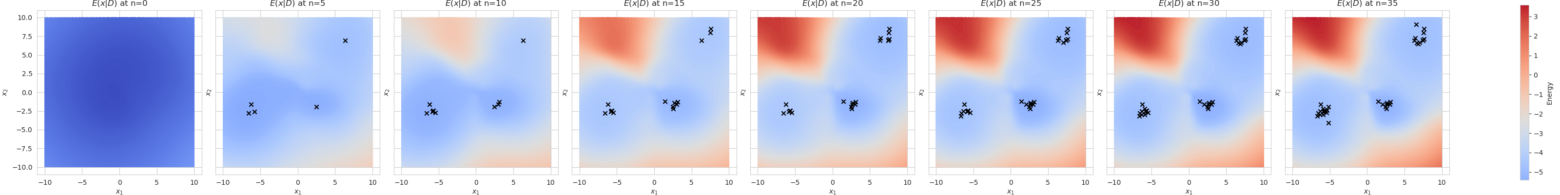
Figure 1: In-Context Learning of Energy Functions. Transformers learn to compute energy functions $E_{\theta}^{ICL}(x|\mathcal{D})$ corresponding to probability distributions $p^{ICL}(x|\mathcal{D})$, where $\mathcal{D}$ are in-context datasets that vary during pretraining. At inference time, when conditioned on a new in-context dataset, the transformer computes a new energy function using fixed network parameters $\theta$. The transformers’ energy landscapes progressively sharpen as additional in-context training data are conditioned upon (left to right).

2 In-Context Learning of Energy Functions

2.1 Motivation for In-Context Learning of Energy Functions

One useful property of associative memory models is their flexibility: the patterns or memories (i.e., training data) $\mathcal{D}\operatorname{\stackrel{{\scriptstyle\text{def}}}{{\;=\;}}}\{{\bm{x}}_{n}\}_{n=1}^{N}$ can be hot-swapped to immediately change the energy landscape. For two examples, the original Hopfield Network (Hopfield, 1982) has energy function:

$$E_{\theta}^{HN}({\bm{x}})\operatorname{\stackrel{{\scriptstyle\text{def}}}{{\;=\;}}}-\frac{1}{2}{\bm{x}}^{T}\Big{(}\frac{1}{N}\sum_{n}{\bm{x}}_{n}{\bm{x}}_{n}^{T}\Big{)}{\bm{x}}$$ (5)

where parameters $\theta$ are the dataset $\mathcal{D}$, and the Modern Continuous Hopfield Network (MCHN) (Ramsauer et al., 2020; Krotov & Hopfield, 2020) has energy function :

$$E_{\theta}^{MCHN}({\bm{x}})\operatorname{\stackrel{{\scriptstyle\text{def}}}{{\;=\;}}}-\frac{1}{\beta}\log\Bigg{(}\sum_{n}\exp\big{(}\beta{\bm{x}}^{T}{\bm{x}}_{n}\big{)}\Bigg{)}+\frac{1}{2}{\bm{x}}^{T}{\bm{x}},$$ (6)

where parameters $\theta$ are the dataset $\mathcal{D}$ and the inverse temperature $\beta>0$. In both examples, the training dataset $\mathcal{D}$ can be replaced with a new dataset $\mathcal{D}^{\prime}$ and the energy landscape immediately adjusts.

In contrast, energy-based models (EBMs) in probabilistic modeling have no equivalent capability because the learned energy $E_{\theta}({\bm{x}})$ depends on pretraining data $\mathcal{D}$ only through the learned neural network parameters $\theta=\theta(\mathcal{D})$ (Du & Mordatch, 2019; Nijkamp et al., 2020; Du et al., 2020a, b, 2021). However, there is no fundamental reason why EBMs cannot be extended to be conditioned on entire datasets as associative memory models often are, and we thus demonstrate how to endow EBMs with such capabilities.

2.2 Learning and Sampling In-Context Learning of Energy Functions

We therefore propose energy-based modeling of dataset-conditioned distributions. This EBM should accept as input an arbitrarily sized dataset $\mathcal{D}$ and a single datum ${\bm{x}}$, and adaptively change its output energy function $E_{\theta}^{ICL}({\bm{x}}|\mathcal{D})$ based on the input dataset without changing its parameters $\theta$. This corresponds to learning the conditional distribution:

$$p_{\theta}^{ICL}({\bm{x}}|\mathcal{D})=\frac{\exp\big{(}-E_{\theta}^{ICL}({\bm{x}}|\mathcal{D})\Big{)}}{Z_{\theta}(\mathcal{D})}$$ (7)

Based on a similarity to in-context learning capabilities of language models (Brown et al., 2020), we call this in-context learning of energy functions (ICL-EBM). We use a transformer (Vaswani et al., 2017) with a causal GPT-like architecture (Radford et al., 2018, 2019). The transformer is trained to minimize the negative log conditional probability, averaging over all possible in-context datasets:

$$\mathcal{L}(\theta)\;\operatorname{\stackrel{{\scriptstyle\text{def}}}{{\;=\;}}}\;\mathbb{E}_{p_{data}}\Bigg{[}\mathbb{E}_{{\bm{x}},\mathcal{D}\sim p_{data}}\Big{[}-\log p_{\theta}^{ICL}({\bm{x}}|\mathcal{D})\Big{]}\Bigg{]}.$$ (8)

Due to the intractable partition function in Eqn. 8, we minimize the loss using contrastive divergence (Hinton, 2002). Letting ${\bm{x}}^{+}$ denote real training data and ${\bm{x}}^{-}$ denote confabulatory data sampled from the learned energy function, the gradient of the loss function is given by:

$$\nabla_{\theta}\mathcal{L}(\theta)=\nabla_{\theta}\,\mathbb{E}_{p_{data}}\Bigg{[}\mathbb{E}_{{\bm{x}}^{+}\mathcal{D}\sim p_{data}}\Big{[}-\log p_{\theta}({\bm{x}}|\mathcal{D})\Big{]}\Bigg{]}$$

$$=\mathbb{E}_{p_{data}}\Bigg{[}\mathbb{E}_{{\bm{x}}^{+}|\mathcal{D}\sim p_{data}}\Big{[}\nabla_{\theta}E_{\theta}^{ICL}({\bm{x}}^{+},\mathcal{D})\Big{]}\Bigg{]}$$

$$-\mathbb{E}_{p_{data}}\Bigg{[}\mathbb{E}_{\mathcal{D}\sim p_{data}}\Big{[}\mathbb{E}_{{\bm{x}}^{-}\sim p_{\theta}^{ICL}({\bm{x}}|\mathcal{D})}\big{[}\nabla_{\theta}E_{\theta}^{ICL}({\bm{x}}^{-}|\mathcal{D})\big{]}\Big{]}\Bigg{]},$$

To sample from the conditional distribution $p_{\theta}({\bm{x}}|\mathcal{D})$, we follow standard practice (Hinton, 2002; Du & Mordatch, 2019; Du et al., 2020b): We first choose $N$ data (deterministically or stochastically) to condition on. We then perform one forward pass through the transformer using inputs $\mathcal{D}$ to compute the energy $E_{\theta}(\mathcal{D})$ corresponding to the marginal $p_{\theta}(\mathcal{D})$, and perform a second forward pass using inputs $\mathcal{D}$ and ${\bm{x}}_{0}^{-}\sim\mathcal{U}$ for some $\mathcal{U}$ to compute the joint energy $E_{\theta}({\bm{x}}_{0}^{-},\mathcal{D})$. The difference $E_{\theta}(\mathcal{D})-E_{\theta}({\bm{x}}_{0}^{-},\mathcal{D})$ is the data-conditioned energy of ${\bm{x}}_{0}^{-}$. We then use Langevin dynamics to iteratively increase the probability of ${\bm{x}}_{0}^{-}$ by sampling with $\omega_{t}\sim\mathcal{N}(0,\sigma^{2})$ and minimizing the energy with respect to ${\bm{x}}_{t}^{-}$ for $t=[T]$ steps:

$${\bm{x}}_{t+1}^{-}\leftarrow{\bm{x}}_{t}^{-}-\alpha\nabla_{{\bm{x}}}\,E_{\theta}^{ICL}({\bm{x}}_{t}^{-},\mathcal{D})+\omega_{t}.$$ (9)

This in-context learning of energy functions is akin to Mordatch (2018), but rather than conditioning on a “mask” and “concepts”, we instead condition on sequences of data from the same distribution and we additionally replace the all-to-all relational network with a causal transformer.

2.3 Experiments for In-Context Learning of Energy Functions

As proof of concept, we train causal transformer-based ICL-EBMs on synthetic datasets. The transformers have $6$ layers, $8$ heads, $128$ embedding dimensions, and GeLU nonlinearities (Hendrycks & Gimpel, 2016). The transformers are pretrained on randomly sampled synthetic 2-dimensional mixture of three Gaussians with uniform mixing proportions with Langevin noise scale $0.01$ and 15 MCMC steps of size $\alpha=3.16$. After pretraining, we then freeze the ICL-EBMs’ parameters and measure whether the model can adapt its energy function to new in-context datasets drawn from the same distribution as the pretraining datasets. The energy landscapes of frozen ICL EBMs display clear signs of in-context learning (Fig. 1). To the best of our knowledge, this is the first instance of in-context learning where the input and output spaces differ, in stark comparison with more common examples of in-context learning such as language modeling (Brown et al., 2020), linear regression (Garg et al., 2022) and image classification (Chan et al., 2022).

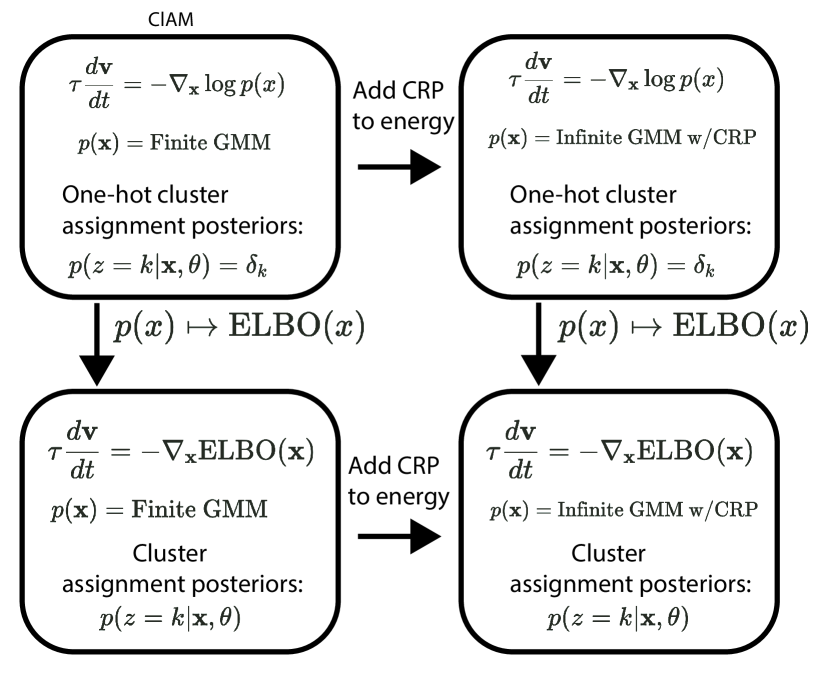
Figure 2: New Nonparametric and Latent Variable Associative Memory Models. We propose new associative memory models that can create new memories using Bayesian nonparametrics (left to right) and can compute proportional cluster assignments using the evidence lower bound (top to bottom). Applying both together results in an associative memory model capable of creating new memories and simultaneously explicitly computing cluster assignment posteriors, with a probability of creating a new memory (i.e., a new cluster centroid).

3 Learning Memories for Associative Memory Models

3.1 Connecting Research on Learning Memories

In many associative memory models, the energy function is defined a priori. However, one might instead learn the energy function. One approach to do so is to transform each datum ${\bm{x}}_{n}$ into a learnt representation $\bm{\xi}_{n}$ that is then dynamically evolved through a classical energy landscape (Ramsauer et al., 2020; Hoover et al., 2023a). A complementary approach is to learn $K$ memories using $N$ data, an approach recently taken by Saha et al. (2023) called Clustering with Associative Memories (ClAM). We show how ClAM is closely connected to probabilistic modeling; by making the connection explicit, we then propose two new associative memory models (Sec. 3.1.1, 3.1.2) as well as a combined form (Sec. 3.1.3). ClAM’s energy function is:

$$E_{\theta}^{ClAM}({\bm{x}})\operatorname{\stackrel{{\scriptstyle\text{def}}}{{\;=\;}}}-\frac{1}{\beta}\log\Bigg{(}\sum_{k}\exp\big{(}-\beta||\bm{\mu}_{k}-{\bm{x}}||^{2}\big{)}\Bigg{)},$$ (10)

where parameters $\theta$ are the learnable memories $\{\bm{\mu}_{k}\}_{k=1}^{K}$ and inverse temperature $\beta$. The dynamics are:

$$\tau\frac{d{\bm{x}}(t)}{dt} =\sum_{k}(\bm{\mu}_{k}-{\bm{x}})\;\mathrm{Softmax}\Big{(}-\beta||\bm{\mu}_{k}-{\bm{x}}||^{2}\Big{)}.$$ (11)

To learn the memories, ClAM perform gradient descent with respect to $\{\bm{\mu}_{k}\}_{k}$ on the reconstruction loss:

$$\mathcal{L}^{ClAM}\Big{(}\{\bm{\mu}_{k}\}_{k}\Big{)}\operatorname{\stackrel{{\scriptstyle\text{def}}}{{\;=\;}}}\sum_{n=1}^{n}\Big{|}\Big{|}{\bm{x}}_{n}-{\bm{x}}_{n}^{\{\bm{\mu}_{k}\}}(T)\Big{|}\Big{|}^{2},$$ (12)

where ${\bm{x}}_{n}^{\{\bm{\mu}_{k}\}}(T)$ is the state of the AM network with memories $\{\bm{\mu}_{k}\}_{k=1}^{K}$ having been initialized at ${\bm{x}}(0)={\bm{x}}_{n}$ and then following the dynamics for $T$ time. This associative memory model has a clear connection to probabilistic modeling as it corresponds exactly to a finite Gaussian mixture model with homogeneous isotropic covariances $\Sigma_{K}=2\beta^{-1}I_{D}$ and uniform mixing proportions $\pi_{k}=1/K$:

$$p_{\theta}^{ClAM}({\bm{x}})=\sum_{k=1}^{K}\mathcal{N}({\bm{x}};\bm{\mu}_{k},\Sigma_{k})\,\pi_{k}.$$

Choosing non-uniform mixing proportions corresponds to ClAM’s “weighted clustering,” and choosing a von Mises-Fisher likelihood corresponds to their “spherical clustering”; one can, of course, choose other likelihoods e.g. Laplace, uniform, Lévy, etc. We also see that the fixed points of the associative memory dynamics are the memories weighted by the cluster assignment posteriors; that is, if the network is initialized at ${\bm{x}}(0)={\bm{x}}$, then ${\bm{x}}^{*}\operatorname{\stackrel{{\scriptstyle\text{def}}}{{\;=\;}}}\sum_{k}p(z=k|{\bm{x}};\theta)\bm{\mu}_{k}$ is a fixed point:

$$\tau\frac{d{\bm{x}}^{*}}{dt} =\Bigg{(}\underbrace{\sum_{k}\bm{\mu}_{k}\mathrm{Softmax}\big{(}-\beta||\bm{\mu}_{k}-{\bm{x}}^{*}||^{2}\big{)}}_{\operatorname{\stackrel{{\scriptstyle\text{def}}}{{\;=\;}}}{\bm{x}}^{*}}$$

$$\quad\quad-{\bm{x}}^{*}\underbrace{\sum_{k}\mathrm{Softmax}\big{(}-\beta||\bm{\mu}_{k}-{\bm{x}}^{*}||^{2}\big{)}}_{=1}\Bigg{)}=0.$$

In the language of probabilistic modeling, ClAM is “Generalized Expectation Maximization (EM)” (Dempster et al., 1977; Xu & Jordan, 1996; Neal & Hinton, 1998; Salakhutdinov et al., 2003) applied to a mixture model. Generalized EM’s two alternating phases correspond to ClAM’s two alternating phases. Generalized EM’s expectation step prescribes increasing the log likelihood with respect to the cluster assignment posterior probabilities, which corresponds to ClAM minimizing its energy function (Eqn. 10) with respect to the particle ${\bm{x}}(t)$ by rolling out the dynamics (Eqn. 11). Generalized EM’s maximization step, which maximizes the log-likelihood with respect to the parameters $\theta$, mirrors ClAM’s shaping of the energy landscape by taking a gradient step with respect to the parameters $\theta$. Thus, ClAM is a dynamical system whose forward dynamics cluster individual data. This is similar to recent nonlinear control work (Romero et al., 2019; Chatterjee et al., 2022), but differs in that ClAM updates the parameters $\theta$ via backpropagation (Rumelhart et al., 1986) rather than in its forward dynamics.

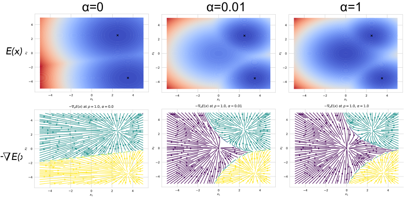
Figure 3: The energy landscape of new memory creation. Left: Finite mixture models can result in each cluster’s basin stretching out infinitely far. Middle and Right: Using the Chinese Restaurant Process, we endow the associative memory model with the ability to create new memories (cluster centroids) if the data is sufficiently far from existing memories: If a datum flows to the origin, we create a new memory for it. Hyperparameter $\alpha$ controls how likely new memories are to be created, with higher $\alpha$ attracting more points to the origin, causing faster cluster creation.

By making this connection, we can now propose two new classes of associative memory models: latent variable and Bayesian nonparametric associative memory models.

3.1.1 Latent Variable Associative Memory Models

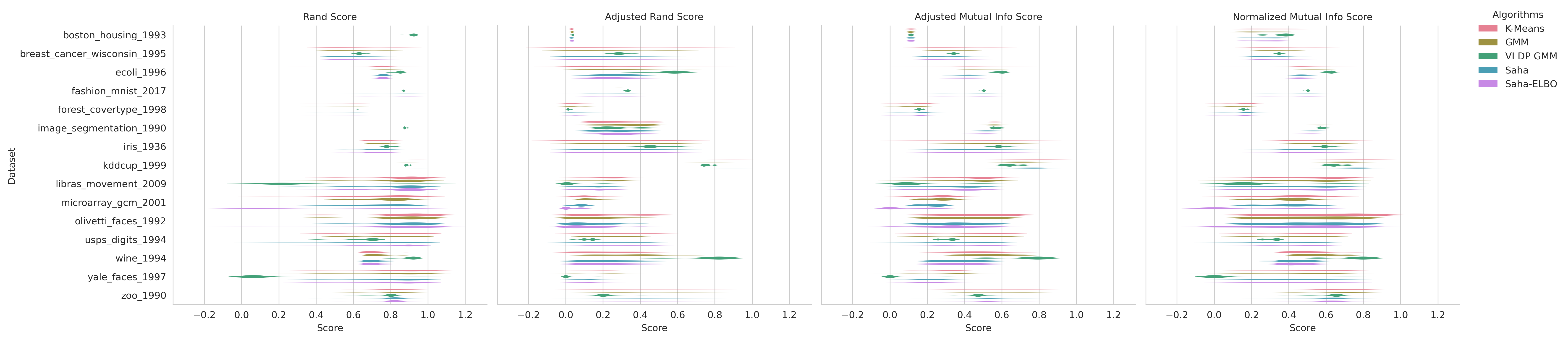
Figure 4: ClAM, ClAM+ELBO, and various baselines’ performance on supervised metrics for standard benchmark datasets. ClAM+ELBO is competitive with ClAM across benchmark tasks in supervised metrics.

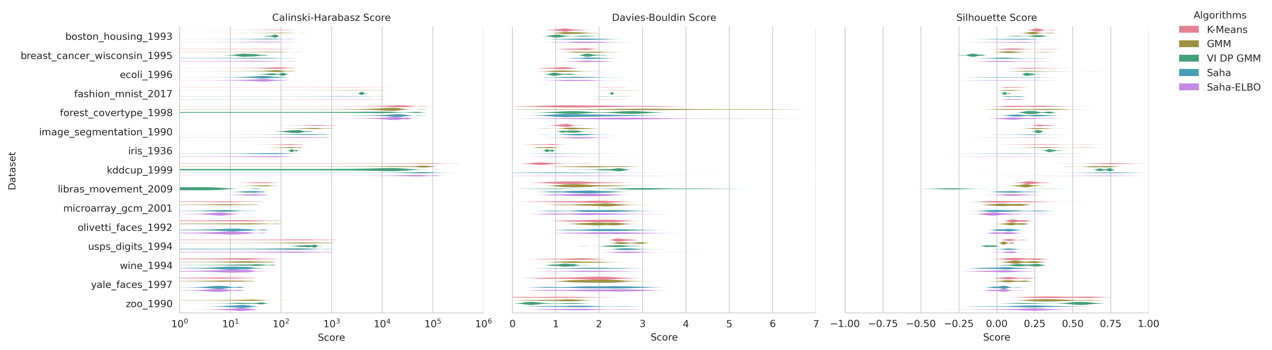
Figure 5: ClAM, ClAM+ELBO, and various baselines’ performance on unsupervised metrics for standard benchmark datasets. ClAM+ELBO is competitive with ClAM across benchmark tasks in unsupervised metrics.

One limitation of ClAM’s associative memory is that, in the context of clustering, it provides no mechanism to obtain the cluster assignment posteriors $p_{\theta}(z=k|{\bm{x}};\theta)$ despite implicitly computing them. Such posteriors are useful for probabilistic uncertainty quantification and also for designing more powerful associative memory networks (Sec. 3.1.2). We propose a new associative memory model that preserves the fixed points and their stability properties but computes the cluster assignment posteriors explicitly by converting the evidence lower bound (ELBO) – a widely used lower bound in probabilistic modeling – into an energy function with corresponding dynamics. Recall that the log likelihood can be lower bounded by Jensen’s inequality:

$$\log p_{\theta}({\bm{x}})^{ClAM} \geq\mathbb{E}_{q(z)}[\log p_{\theta}({\bm{x}},z=k)]+H[q(z)],$$

where $H(\cdot)$ is the entropy. Denote $q(z)$ with the probability vector ${\bm{q}}\in\Delta^{K-1}$ and define the energy function:

$$E_{\theta}^{ClAM+ELBO}({\bm{q}}) \operatorname{\stackrel{{\scriptstyle\text{def}}}{{\;=\;}}}-\sum_{k=1}^{K}{\bm{q}}_{k}\log p_{\theta}({\bm{x}},z=k)+H({\bm{q}})$$

To ensure that ${\bm{q}}(t)$ remains a probability vector, we reparameterize ${\bm{q}}(t)$ using ${\bm{v}}(t)\in\mathbb{R}^{K}$ with ${\bm{q}}(t)=\mathrm{Softmax}({\bm{v}}(t))$. This yields an associative memory model where the state ${\bm{v}}(t)$ lives in the number-of-clusters-dimensional logit space $\mathbb{R}^{K}$ rather than data space $\mathcal{X}$. Recalling that the gradient of probability vector ${\bm{q}}$ with respect to its logits ${\bm{v}}$ can be expressed in matrix notation as $\nabla_{{\bm{v}}}{\bm{q}}=\operatorname{\text{diag}}({\bm{q}})-{\bm{q}}{\bm{q}}^{T}\in\mathbb{R}^{K\times K}$, the dynamics in logit space are:

$$\tau \frac{d}{dt}{\bm{v}}(t)\operatorname{\stackrel{{\scriptstyle\text{def}}}{{\;=\;}}}-\nabla_{{\bm{v}}}E_{\theta}^{ClAM+ELBO}({\bm{q}}({\bm{v}}(t)))$$ (13)

$$=\Big{(}\operatorname{\text{diag}}({\bm{q}})-{\bm{q}}{\bm{q}}^{T}\Big{)}\Big{(}\log p_{\theta}({\bm{x}},z)-\log{\bm{q}}-\bm{1}\Big{)}$$ (14)

In ${\bm{q}}$ space, these dynamics have a single fixed point corresponding to the cluster assignment posteriors: ${\bm{q}}^{*}=p(z=k|{\bm{x}};\theta)$. However due to the invariance of Softmax to constant offsets, the dynamics do not have a single fixed point but rather an invariant set in ${\bm{v}}$ space: $\mathrm{Softmax}({\bm{v}}+c)_{k}=(\exp{\bm{v}}_{k}\exp c)/(\sum_{i}\exp{\bm{v}}_{i}\exp c)=\exp{\bm{v}}_{k}/\sum_{i}\exp{\bm{v}}_{i}=\mathrm{Softmax}({\bm{v}})_{k}$. This implies the same symmetry exists in the energy function, $E_{\theta}^{ClAM+ELBO}({\bm{v}}+c)=E_{\theta}^{ClAM+ELBO}({\bm{v}})$, thus all minima ${\bm{v}}^{*}$ (the fixed points of the energy function) are in fact invariant sets ${\bm{v}}^{*}+\alpha\mathbf{1}$, with $\alpha\in\mathbb{R}$. Like ClAM, convergence to a local minimum is guaranteed because the energy is monotonically non-increasing over time:

$$\frac{d}{dt}E({\bm{q}}({\bm{v}}(t))) =\nabla_{{\bm{v}}}E^{ClAM+ELBO}({\bm{q}}({\bm{v}}(t)))\cdot\frac{d}{dt}{\bm{v}}(t)$$

$$=-\nabla_{{\bm{v}}}E({\bm{q}}({\bm{v}}(t))\cdot\nabla_{{\bm{v}}}E({\bm{q}}({\bm{v}}(t)))$$

$$=-||\nabla_{{\bm{v}}}E({\bm{q}}({\bm{v}}(t)))||^{2}$$

Empirically, we find that ClAM-ELBO is competitive with ClAM across a wide range of benchmarks under both supervised and unsupervised metrics (Fig. 4, Fig. 5).

3.1.2 Bayesian Nonparametric Associative Memory Models

Based on the connection to probabilistic modeling, one can also learn energy functions where the number of memories is not fixed but rather learned as necessitated by the data $\mathcal{D}$. We may motivate this approach both biologically and computationally. Biologically, animals create new memories throughout their lives, and the process by which these processes occur are fundamental topics in experimental and computational neuroscience alike (Sec. 6). Computationally, in the context of clustering, choosing the right number of clusters is a perennial problem (Thorndike, 1953; Rousseeuw, 1987; Bischof et al., 1999; Pelleg et al., 2000; Tibshirani et al., 2001; Sugar & James, 2003; Hamerly & Elkan, 2003; Kulis & Jordan, 2012).

To create an AM network with the ability to create new memories, we propose leveraging Bayesian nonparametrics based on combinatorial stochastic processes (Pitman, 2006). Specifically, we will use the Chinese Restaurant Process (CRP) (Blackwell & MacQueen, 1973; Antoniak, 1974; Aldous et al., 1985; Teh et al., 2010). The CRP defines a probability distribution over partitions of a set that can then be used as an “infinite”-dimensional prior over the number of clusters as well as a prior over the number of data per cluster. Specifically, let $\alpha>0,d\in[0,1)$ and $K_{<n}\operatorname{\stackrel{{\scriptstyle\text{def}}}{{\;=\;}}}\max\{z_{1},...,z_{n-1}\}$ denote the number of clusters after the first $n-1$ data. Then $CRP(\alpha,d)$ defines a conditional prior distribution on cluster assignments:

$$p(z_{n}=k|z_{<n},\alpha,d)\;\operatorname{\stackrel{{\scriptstyle\text{def}}}{{\;=\;}}}$$

$$\frac{1}{n-1+\alpha}\begin{cases}-d+\sum_{n^{\prime}<n}\mathbbm{I}(z_{n^{\prime}}=k)&\text{ if }1\leq k\leq K_{<n}^{+}\\ \alpha+d\cdot K_{<n}^{+}&\text{ if }k=K_{<n}^{+}+1\\ 0&\text{otherwise}\end{cases}$$

The hyperparameter $\alpha>0$ controls how quickly new clusters form, and the hyperparameter $d\in[0,1)$ controls how quickly existing memories accumulate mass. We propose using the CRP to define a novel associative memory model that creates new memories. Let $\theta$ denote the model parameters: $K^{+}$ is the number of clusters, $\{\tilde{\pi}_{k}\}_{k=1}^{K^{+}}$ are the number of data assigned to each existing cluster, and $\{\bm{\mu}_{k},\Sigma_{k}\}_{k=1}^{K^{+}}$ are the means and covariances of the clusters. Then, assuming an isotropic Gaussian likelihood $\Sigma_{k}=2\beta^{-1}I_{D}$ and assuming an isotropic Gaussian prior on the cluster means $\bm{\mu}_{k}\sim\mathcal{N}(\bm{0},2\rho^{-1}I_{D})$, the probability of datum ${\bm{x}}$ is:

$$p_{\theta}^{ClAM+CRP}({\bm{x}})$$

$$\;\operatorname{\stackrel{{\scriptstyle\text{def}}}{{\;=\;}}}\;p({\bm{x}}|z=K^{+}+1;\theta)\,p(z=K^{+}+1;\theta)$$

$$\quad\quad+\sum_{k=1}^{K^{+}}p({\bm{x}}|z=k;\theta)\,p(z=k;\theta)$$

$$=\;\mathcal{N}({\bm{x}};\bm{0},2\,(\rho^{-1}+\beta^{-1})I_{D})\frac{\alpha+K^{+}d}{\alpha-1+\sum_{k=1}^{K^{+}}\tilde{\pi}_{k}}$$

$$\quad\quad+\sum_{k=1}^{K^{+}}\mathcal{N}({\bm{x}};\bm{\mu}_{k},2\beta^{-1}I_{D})\,\frac{\tilde{\pi}_{k}-d}{\alpha-1+\sum_{k=1}^{K^{+}}\tilde{\pi}_{k}}.$$

Using the same process as before, we can convert the probability distribution into an energy function via the inverse temperature-scaled negative log likelihood:

$$E_{\theta}^{ClAM+CRP}({\bm{x}})\operatorname{\stackrel{{\scriptstyle\text{def}}}{{\;=\;}}}$$

$$-\frac{1}{\beta}\log\Bigg{(}\exp\Big{(}-(\beta^{-1}+\rho^{-1})^{-1}||\bm{0}-{\bm{x}}||^{2}\Big{)}(\alpha+K^{+}d)$$

$$\quad\quad\quad\quad\quad+\sum_{k=1}^{K^{+}}\exp\Big{(}-\beta||\bm{\mu}_{k}-{\bm{x}}||^{2}\Big{)}(\tilde{\pi}_{k}-d)\Bigg{)}$$

The associative memory dynamics are defined as:

$$\tau\frac{d{\bm{x}}}{dt}\;\operatorname{\stackrel{{\scriptstyle\text{def}}}{{\;=\;}}}\;-\frac{1}{2}\nabla_{{\bm{x}}}E_{\theta}^{ClAM+CRP}({\bm{x}})$$

We call this ClAM+CRP.

3.1.3 Nonparametric Latent Variable Energy Functions

One can straightforwardly combine the proposed latent variable associative memory model (Sec. 3.1.1) with the nonparametric associative memory (Sec. 3.1.2) to yield a nonparametric latent variable associative memory model:

$$E_{\theta}^{ClAM+CRP+ELBO}({\bm{q}})\operatorname{\stackrel{{\scriptstyle\text{def}}}{{\;=\;}}}$$

$$\ -\sum_{k=1}^{K}{\bm{q}}_{k}\log p_{\theta}^{CRP}({\bm{x}},z=k)+\sum_{k=1}^{K}{\bm{q}}_{k}\log{\bm{q}}_{k}.$$

Interestingly, ClAM+CRP+ELBO shares some striking similarities with memory engrams (Josselyn & Tonegawa, 2020), an exciting new area of experimental neuroscience (Yiu et al., 2014; Rashid et al., 2016; Park et al., 2016; Lisman et al., 2018; Pignatelli et al., 2019; Lau et al., 2020; Jung et al., 2023) . Neurobiologically, we can view these dynamics as $K$ memory engrams that are self-excitatory and mutually inhibitory, with interactions given by $\operatorname{\text{diag}}({\bm{q}})-{\bm{q}}{\bm{q}}^{T}$. We intend to explore this connection in subsequent work.

4 Capacity, Retrieval and Memory Cliffs of Gaussian Kernel Density Estimators

An interesting problem commonly solved in the associative memory literature is analytically characterizing the memory retrieval, capacity, and failure behavior of memory systems (Gardner, 1988; Krotov & Hopfield, 2016; Demircigil et al., 2017; Chaudhuri & Fiete, 2019; Lucibello & Mézard, 2023). In this section, we use such tools to study memory properties of kernel density estimators (KDEs), a widely used tool from probabilistic modeling (Parzen, 1962; Rosenblatt, 1956; Epanechnikov, 1969; Wand & Jones, 1994; Sheather & Jones, 1991; Hastie et al., 2009). Given $N$ i.i.d. samples $\mathcal{D}\operatorname{\stackrel{{\scriptstyle\text{def}}}{{\;=\;}}}\{{\bm{x}}_{n}\}_{n=1}^{N}\in\mathbb{R}^{D}$ from some unknown distribution, a kernel density estimator (KDE) estimates the unknown distribution via:

$$\hat{p}_{K,h}^{KDE}({\bm{x}})\operatorname{\stackrel{{\scriptstyle\text{def}}}{{\;=\;}}}\frac{1}{Nh}\sum_{n=1}^{N}K\Big{(}\frac{{\bm{x}}-{\bm{x}}_{n}}{h}\Big{)},$$

with kernel function $K(\cdot)$ and bandwidth $h$. The energy is defined as the negative log probability of the KDE:

$$E_{K,h}^{KDE}({\bm{x}})\operatorname{\stackrel{{\scriptstyle\text{def}}}{{\;=\;}}}-\log\bigg{(}\hat{p}_{K,h}^{KDE}({\bm{x}})\bigg{)},$$ (15)

KDEs explicitly construct basin-like structures around each training datum, and thus can be viewed as memorizing the training data. We say that a pattern ${\bm{x}}_{n}$ has been stored if there exists a ball with radius $R_{n}$, $S_{n}\operatorname{\stackrel{{\scriptstyle\text{def}}}{{\;=\;}}}\{{\bm{x}}\in\mathbb{R}^{D}:||{\bm{x}}-{\bm{x}}_{n}||_{2}\leq R_{n}\}$, centered at ${\bm{x}}_{n}$ such that every point within $S_{n}$ converges to some fixed point ${\bm{x}}_{n}^{*}\in S_{n}$ under the defined dynamics. The balls for different patterns must be disjoint. We show here that KDEs have a finite memory storage and retrieval capacity (Fig. 6), by establishing a connection between the commonly used Gaussian KDE and the Modern Continuous Hopfield Network (MCHN) developed by Ramsauer et al. (2020). This connection allows us to extend the capacity and convergence properties of the MCHN to the Gaussian KDE, showing that it has exponential storage capacity in the data dimensionality. The widely used Gaussian KDE uses a Gaussian kernel with length scale (standard deviation) $\sigma$. Its energy is:

$$E_{\text{Gauss},\sigma}({\bm{x}})\operatorname{\stackrel{{\scriptstyle\text{def}}}{{\;=\;}}}-\log\Bigg{(}\sum_{n=1}^{N}\exp\bigg{(}-\frac{1}{2\sigma^{2}}||{\bm{x}}-{\bm{x}}_{n}||^{2}\bigg{)}\Bigg{)}.$$

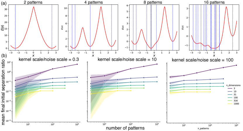
Figure 6: KDE as associative memory: memory capacity limits. (a) As more patterns are added, their energy basins (minima) merge, leaving us unable to retrieve them individually. (b) We quantify how well we can retrieve data by calculating the mean ratio of the distance between queries and their corresponding patterns after undergoing dynamics to before. We then normalize this ratio by the average distance of patterns. The smaller this ratio is, the closer the queries have converged to their corresponding patterns. We see that increasing the number of patterns results in poorer retrieval, while increasing the number of dimensions results in better retrieval.

The dynamics of the Gaussian KDE are defined according to gradient descent on the energy landscape. For an arbitrary step size $\alpha$ we define the update rule:

$${\bm{x}}^{(i+1)}={\bm{x}}^{(i)}-\alpha\nabla E_{\text{Gauss},\sigma}({\bm{x}}^{(i)}).$$

In App. A, we prove that the energy and dynamics of the Gaussian KDE is exactly equivalent to the energy and update rule of the MCHN of Ramsauer et al. (2020). Given the equivalence, we can characterize the capabilities and limitations of kernel density estimators in the same way as derived for MCHNs by Ramsauer et al. (2020). Ergo, the capacity of the Gaussian KDE is shown to be:

$$C_{\text{Gauss}}=2^{2(D-1)}.$$ (16)

In Fig. 6. (b), we demonstrate numerically that Gaussian KDEs exhibit better retrieval at higher data dimensions and worse retrieval with more patterns.

5 A Theoretical Justification for Normalization before Self-Attention

Next, we discover a way to understand the interaction between self-attention and normalization in transformers (Vaswani et al., 2017). The well-known equation for self-attention is:

$$\text{SA}(\mathbf{q},K,V)\operatorname{\stackrel{{\scriptstyle\text{def}}}{{\;=\;}}}V\;\mathrm{Softmax}\;(K{\bm{q}}).$$

Here, $V\in\mathbb{R}^{d\times d},K\in\mathbb{R}^{d\times d},q\in\mathbb{R}^{d}$. Previous work has connected self-attention to Hopfield networks (Ramsauer et al., 2020; Millidge et al., 2022). However, transformers are not purely stacked self-attention layers; among many components, practitioners have found that applying normalization (e.g., LayerNorm (Ba et al., 2016), RMS Norm (Zhang & Sennrich, 2019)) before self-attention significantly improves performance (Baevski & Auli, 2018; Child et al., 2019; Wang et al., 2019; Xiong et al., 2020).

What effect does this composition of pre-normalization and self-attention have? We show that the two together approximate clustering on the hypersphere using a mixture of inhomogeneous von Mises-Fisher (vMF) distributions (Fisher, 1953). For concreteness, we consider LayerNorm, although RMS norm produces the same qualitative result.

$$LN_{\bm{\gamma},\bm{\delta}}({\bm{x}})\quad\operatorname{\stackrel{{\scriptstyle\text{def}}}{{\;=\;}}}\quad\bm{\gamma}\odot\frac{{\bm{x}}-{\bm{m}}}{\sqrt{\sigma^{2}+\epsilon}}+\bm{\delta},$$ (17)

where $\epsilon$ is a small constant for numerical stability and $\odot$ denotes elementwise multiplication. Recall that the vMF density function with unit vector ${\bm{m}}_{i}\in\mathbb{R}^{D},||{\bm{m}}_{i}||_{2}=1$ and concentration $\kappa_{i}\geq 0$ is:

$$p({\bm{x}};{\bm{m}}_{i},\kappa_{i})\propto\exp(\kappa_{i}\,{\bm{m}}_{i}\cdot{\bm{x}}).$$ (18)

Define $\tilde{{\bm{q}}}$ as the pre-shifted and scaled query i.e., ${\bm{q}}\operatorname{\stackrel{{\scriptstyle\text{def}}}{{\;=\;}}}\bm{\gamma}\odot\tilde{{\bm{q}}}+\bm{\delta}$, with $||\tilde{{\bm{q}}}||_{2}\approx 1$. The $i^{\text{th}}$ element in the numerator of the softmax is:

$$\exp({\bm{k}}_{i}\cdot{\bm{q}})=\exp({\bm{k}}_{i}\cdot(\bm{\gamma}\odot\tilde{{\bm{q}}}+\bm{\delta}))$$

$$=\exp\Bigg{(}\underbrace{||({\bm{k}}_{i}\odot\bm{\gamma})||_{2}}_{=\kappa_{i}}\underbrace{\frac{{\bm{k}}_{i}\odot\bm{\gamma}}{||{\bm{k}}_{i}\odot\bm{\gamma}||}}_{={\bm{m}}_{i}}\;\cdot\;\tilde{{\bm{q}}}\Bigg{)}\;\underbrace{\exp\Bigg{(}{\bm{k}}_{i}\cdot\bm{\delta}\Bigg{)}}_{=\pi_{i}}.$$

Thus, LayerNorm followed by self-attention is equivalent to clustering with inhomogeneous vMF likelihoods and with (unnormalized) mixing proportions determined by the exponentiated inner products between the keys and the LayerNorm bias. A related commentary about the interaction between pre-LayerNorm and self-attention has been made before (Bricken & Pehlevan, 2021), albeit in a non-clustering and non-probabilistic context. This perspective suggests an unnecessary complexity exists in modern transformers between the keys $\{{\bm{k}}_{i}\}$, scale $\bm{\gamma}$ and shift $\bm{\delta}$ in a way that might hamper expressivity. Specifically, if pre-LayerNorm composed with self-attention is indeed performing clustering, then each key ${\bm{k}}_{i}$ is controlling both the concentration of the vMF likelihood as well as the mixing proportion $\pi_{i}$, and all keys must interact with the same scale $\bm{\gamma}$ and shift $\bm{\delta}$.

Further, recent work (Dehghani et al., 2023) has found that adding LayerNorm on the queries and keys stabilizes learning in ViTs and Wortsman et al. (2023) shows that this operation allows for training with large learning rates while avoiding instabilities (Zhai et al., 2023). Our proposed modification of the queries: ${\bm{q}}\mapsto\bm{\gamma}\odot\tilde{{\bm{q}}}+\bm{\delta}$ indeed is equivalent to transforming ${\bm{q}}\mapsto\text{LN}_{\gamma,\delta}({\bm{q}})=\bm{\gamma}\odot\frac{{\bm{q}}-{\bm{m}}}{\sqrt{\sigma^{2}+\epsilon}}+\bm{\delta}$.

6 Discussion

Associative memory and probabilistic modeling are two foundational fields of artificial intelligence that have remained (largely) unconnected for too long. While recent work has made good steps to demonstrate connections, e.g., to diffusion models (Ambrogioni, 2023; Hoover et al., 2023b), many more meaningful connections exist that our work hopefully demonstrates and inspires.

Appendix A Capacity, Retrieval Errors and Memory Cliffs of Gaussian Kernel Density Estimators

We characterize the capacity and memory cliffs of kernel density estimators, i.e. how much data can be successfully retrieved by following the negative gradient of the log probability, and what happens when that limit is exceeded? Suppose we have $N$ training data $\{{\bm{x}}_{n}\}_{n=1}^{N}\in\mathbb{R}^{D}$, and we consider the estimated probability distribution by a kernel density estimator (KDE):

$$\hat{p}_{K,h}({\bm{x}})\operatorname{\stackrel{{\scriptstyle\text{def}}}{{\;=\;}}}\frac{1}{Nh}\sum_{n=1}^{N}K\Big{(}\frac{{\bm{x}}-{\bm{x}}_{n}}{h}\Big{)},$$ (19)

with kernel function $K(\cdot)$ and bandwidth $h$. The energy is defined as the negative log probability of the KDE:

$$E_{K,h}({\bm{x}})\operatorname{\stackrel{{\scriptstyle\text{def}}}{{\;=\;}}}-\log(\hat{p}_{K,h}({\bm{x}}))=-\log\Bigg{(}\sum_{n=1}^{N}K\Big{(}\frac{{\bm{x}}-{\bm{x}}_{n}}{h}\Big{)}\Bigg{)}+C,$$ (20)

where $C$ is a constant that will not affect dynamics and will be omitted moving forward. To characterize the capacity and failure modes of kernel density estimators, we begin with relevant definitions (many from (Ramsauer et al., 2020)).

Definition A.1 (Separation of Patterns).

The separation $\Delta_{n}$ of a pattern (i.e. a training datum) ${\bm{x}}_{n}$ from the other patterns is defined as one-half the squared distance to the closest training datum:

$$\Delta_{n}\operatorname{\stackrel{{\scriptstyle\text{def}}}{{\;=\;}}}\frac{1}{2}\cdot\min_{n^{\prime}\neq n}||{\bm{x}}_{n}-{\bm{x}}_{n^{\prime}}||^{2}.$$

Definition A.2 (Pattern Storage).

We say that a pattern ${\bm{x}}_{n}$ has been stored if there exists a ball with radius $R_{n}$, $S_{n}\operatorname{\stackrel{{\scriptstyle\text{def}}}{{\;=\;}}}\{{\bm{x}}\in\mathbb{R}^{D}:||{\bm{x}}-{\bm{x}}_{n}||_{2}\leq R_{n}\}$, centered at ${\bm{x}}_{n}$ such that every point within $S_{n}$ converges to some fixed point ${\bm{x}}_{n}^{*}\in S_{n}$ under the defined dynamics. This point ${\bm{x}}_{n}^{*}$ is not necessarily the training point ${\bm{x}}_{n}$. The balls associated with different patterns must be disjoint, i.e. $\forall n^{\prime}\neq n:S_{n^{\prime}}\cap S_{n}=\emptyset$. The value $R_{n}$ is called the radius of convergence.

Definition A.3 (Retrieval Error).

For a stored pattern ${\bm{x}}_{n}$, let $S_{n}$ be the ball around ${\bm{x}}_{n}$ as defined in A.2. By definition A.2, every point within the $S_{n}$ must converge to some ${\bm{x}}_{n}^{*}$. We define the retrieval error to be $||{\bm{x}}_{n}-{\bm{x}}_{n}^{*}||$.

Definition A.4 (Storage Capacity).

The storage capacity of a particular associative memory model is the number of patterns $C$ such that all $C$ patterns ${\bm{x}}_{1},...,{\bm{x}}_{C}$ are stored under Def. A.2.

Definition A.5 (Largest Norm of Training Data).

We define $M$ as the largest $L^{2}$ norm of our training data:

$$M=\max_{n}||{\bm{x}}_{n}||_{2}.$$

A.1 Kernel Density Estimator with a Gaussian Kernel

We begin by studying the widely used Gaussian KDE with length scale (standard deviation) $\sigma$. Its energy function is:

$$E_{\text{Gauss},\sigma}({\bm{x}})\operatorname{\stackrel{{\scriptstyle\text{def}}}{{\;=\;}}}-\log\Bigg{(}\sum_{n=1}^{N}\exp\bigg{(}-\frac{1}{2\sigma^{2}}||{\bm{x}}-{\bm{x}}_{n}||^{2}\bigg{)}\Bigg{)}.$$ (21)

To study the capacity, retrieval error and memory cliff of the Gaussian KDE, it will be helpful to briefly summarize the modern continuous Hopfield network (MCHN) of Ramsauer et al. (2020).

Definition A.6 (MCHN Energy Function).

The MCHN energy function is given as

$$E_{\text{MCHN}}({\bm{x}})\operatorname{\stackrel{{\scriptstyle\text{def}}}{{\;=\;}}}-\beta^{-1}\log\Bigg{(}\sum_{n=1}^{N}\exp\bigg{(}\beta{\bm{x}}_{n}^{T}{\bm{x}}\bigg{)}\Bigg{)}+\beta^{-1}\log(N)+\frac{1}{2}{\bm{x}}^{T}{\bm{x}}+\frac{1}{2}M^{2}$$ (22)

where $\beta$ is the inverse temperature.

Definition A.7 (MCHN Dynamics).

Defining the matrix ${\mathbf{X}}$ whose columns are our training points ${\bm{x}}_{n}$:

$${\mathbf{X}}\operatorname{\stackrel{{\scriptstyle\text{def}}}{{\;=\;}}}\begin{bmatrix}\vline\;\;\;\;\vline\;\;\;\;\;\;\;\;\;\;\;\;\vline\\ {\bm{x}}_{1}\;{\bm{x}}_{2}\;\dots\;{\bm{x}}_{N}\\ \vline\;\;\;\;\vline\;\;\;\;\;\;\;\;\;\;\;\;\vline\end{bmatrix},\in\mathbb{R}^{D\times N},$$

the update rule introduced by Ramsauer et al. (2020) is defined to be

$${\bm{x}}^{(i+1)}={\mathbf{X}}\mathrm{Softmax}\bigg{(}\beta{\mathbf{X}}^{T}{\bm{x}}^{(i)}\bigg{)},$$

which corresponds to the Concave-Convex Procedure (CCCP) for minimizing the energy function in A.6

To calculate the convergence and capacity properties of the MCHN, Ramsauer et al. (2020) assume that all the training points lie on a sphere.

Assumption A.8 (All training points lie on a sphere).

Recall that $M$ is defined as the largest norm of our training data. Moving forward, we assume that the points ${\bm{x}}_{1},...,{\bm{x}}_{N}$ are distributed over a sphere of radius $M$, i.e. that

$$||{\bm{x}}_{1}||=\dots=||{\bm{x}}_{N}||=M.$$

Next, we will show that under assumption A.8, the Gaussian KDE has identical energy and dynamics to the MCHN. Consequently, we are able to extend the capacity and convergence properties of the MCHN derived by Ramsauer et al. (2020) to the Gaussian KDE, showing that it has exponential storage capacity in $D$, the number of dimensions of our data.

Theorem A.9.

The Gaussian KDE energy function is equivalent to the MCHN energy function.

Proof.

We begin by simplifying the MCHN energy equation in A.6. We have

$$\begin{split}E_{\text{MCHN}}({\bm{x}})&=-\beta^{-1}\log\Bigg{(}\sum_{n=1}^{N}\exp\bigg{(}\beta{\bm{x}}_{n}^{T}{\bm{x}}\bigg{)}\Bigg{)}+\beta^{-1}\log(N)+\frac{1}{2}{\bm{x}}^{T}{\bm{x}}+\frac{1}{2}M^{2}\\ &=-\beta^{-1}\log\Bigg{(}\sum_{n=1}^{N}\exp\bigg{(}-\frac{1}{2}\beta\Big{(}M^{2}-||{\bm{x}}_{n}||^{2}\Big{)}\bigg{)}\exp\bigg{(}-\frac{1}{2}\beta||{\bm{x}}-{\bm{x}}_{n}||^{2}\bigg{)}\Bigg{)}+\beta^{-1}\log(N).\end{split}$$

Under assumption A.8, and using inverse temperature $\beta=\frac{1}{\sigma^{2}}$, we can further simplify this equation to get

$$E_{\text{MCHN}}({\bm{x}})=-\sigma^{2}\log\Bigg{(}\sum_{n=1}^{N}\exp\bigg{(}-\frac{1}{2\sigma^{2}}||{\bm{x}}-{\bm{x}}_{n}||^{2}\bigg{)}\Bigg{)}+\sigma^{2}\log(N),$$ (23)

which is a scaled and shifted version of the energy function in 21. Ergo, the Gaussian KDE energy function is equivalent to the MCHN energy function. ∎

Theorem A.10.

The Gaussian KDE with appropriate step size has identical dynamics to the MCHN.

Proof.

For the Gaussian KDE in 21, the dynamics are defined by gradient descent on the energy landscape with step size $\alpha$:

$$\begin{split}{\bm{x}}^{(i+1)}&={\bm{x}}^{(i)}-\alpha\nabla E_{\text{Gauss},\sigma}({\bm{x}}^{(i)})\\ &={\bm{x}}^{(i)}-\frac{\alpha}{\sigma^{2}}\cdot\frac{\sum_{n=1}^{N}\exp\bigg{(}-\frac{1}{2\sigma^{2}}||{\bm{x}}^{(i)}-{\bm{x}}_{n}||^{2}\bigg{)}({\bm{x}}^{(i)}-{\bm{x}}_{n})}{\sum_{n=1}^{N}\exp\bigg{(}-\frac{1}{2\sigma^{2}}||{\bm{x}}^{(i)}-{\bm{x}}_{n}||^{2}\bigg{)}}.\end{split}$$ (24)

Using the assumption A.8, we can further simplify the exponent to get

$$||{\bm{x}}^{(i)}-{\bm{x}}_{n}||^{2}=||{\bm{x}}^{(i)}||^{2}+M^{2}-2{\bm{x}}_{n}^{T}{\bm{x}}^{(i)}.$$

Substituting in 24, and canceling out the common factors we get:

$${\bm{x}}^{(i+1)}={\bm{x}}^{(i)}-\frac{\alpha}{\sigma^{2}}\cdot\frac{\sum_{n=1}^{N}\exp\bigg{(}\frac{1}{\sigma^{2}}{\bm{x}}_{n}^{T}{\bm{x}}^{(i)}\bigg{)}({\bm{x}}^{(i)}-{\bm{x}}_{n})}{\sum_{n=1}^{N}\exp\bigg{(}\frac{1}{\sigma^{2}}{\bm{x}}_{n}^{T}{\bm{x}}^{(i)}\bigg{)}}.$$

Choosing step size $\alpha=\sigma^{2}$, we get the update rule:

$$\begin{split}{\bm{x}}^{(i+1)}&={\bm{x}}^{(i)}-{\bm{x}}^{(i)}+\frac{\sum_{n=1}^{N}{\bm{x}}_{n}\exp\bigg{(}\frac{1}{\sigma^{2}}{\bm{x}}_{n}^{T}{\bm{x}}^{(i)}\bigg{)}}{\sum_{n=1}^{N}\exp\bigg{(}\frac{1}{\sigma^{2}}{\bm{x}}_{n}^{T}{\bm{x}}^{(i)}\bigg{)}}\\ &=\sum_{n=1}^{N}{\bm{x}}_{n}\mathrm{Softmax}\bigg{(}\frac{1}{\sigma^{2}}{\bm{x}}_{n}^{T}{\bm{x}}^{(i)}\bigg{)}\\ &={\mathbf{X}}\mathrm{Softmax}\bigg{(}\beta{\mathbf{X}}^{T}{\bm{x}}^{(i)}\bigg{)},\end{split}$$ (25)

which is precisely the update rule described in A.7. ∎

We have demonstrated an equivalence between the energy functions and update rules of MCHNs and Gaussian KDEs. We now apply convergence and storage capacity analysis for MCHNs to Gaussian KDEs Ramsauer et al. (2020).

Proposition A.11.

If the training points are well separated, the Gaussian KDE has a radius of convergence equal to $\frac{\sigma^{2}}{NM}$.

Proof.

We assume that the data ${\bm{x}}_{n}$ is well-separated. Concretely, we have:

Assumption A.12 (Well-Separated Data).

$$\Delta_{n}\geq\frac{2\sigma^{2}}{N}+\sigma^{2}\log\bigg{(}\frac{2}{\sigma^{2}}(N-1)NM^{2}\bigg{)}.$$ (26)

Defining the ball around ${\bm{x}}_{n}$:

$$S_{n}\operatorname{\stackrel{{\scriptstyle\text{def}}}{{\;=\;}}}\left\{{\bm{x}}\;\middle|\;\;||{\bm{x}}-{\bm{x}}_{n}||\leq\frac{\sigma^{2}}{NM}\right\},$$

Ramsauer et al. (2020) show that our update rule in 25 is a contraction mapping over the ball $S_{n}$. Thus, by Banach’s fixed point theorem, the update rule converges to a fixed point within the ball after sufficient iterations. Thus, by our definition of storage and retrieval, the point ${\bm{x}}_{n}$ will be stored and the radius of $S_{n}$ gives the radius of convergence:

$$R_{n}=\frac{\sigma^{2}}{NM}.$$ (27)

∎

Intuitively, if our patterns get too close, their corresponding basins in the energy function merge, leaving us unable to retrieve either of them individually. This can be seen in the lower panel of Fig. 7

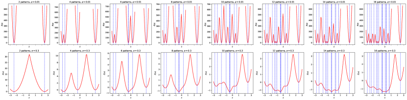
Figure 7: Energy landscape under different numbers of patterns, with two different standard deviation values $\sigma$. The basins for different patterns are more likely to merge when the Gaussian has a larger standard deviation, and when the patterns are too close together. The latter is likely to happen when we attempt to store too many patterns in a finite space. When two basins merge, we are unable to retrieve the corresponding patterns individually.

Assumption A.12 establishes a lower bound for just how close the patterns can get without their energy basins merging. This depends on the standard deviation of the Gaussian, number of data points, and the radius of the sphere they are distributed over. Intuitively, if the standard deviation of the Gaussian is large, the basins are more likely to merge, and thus the lower bound for $\Delta_{n}$ increases with $\sigma$. In Fig. 7, we can observe the effects of $\sigma$ on the energy landscape. A smaller $\sigma$ allows for patterns to be closer before their basins merge.

Additionally, notice that for large $N$ (meaning that we have a lot of training points), the lower bound for $\Delta_{n}$ increases with $N$, signifying the fact that the dynamics near each basin can be overwhelmed by the collective effects of multiple other basins. Therefore, the more training points we have, the more we need to separate out the training points in order to safely retrieve them.

Now, we turn our attention to the storage capacity of the Gaussian KDE.

Proposition A.13.

If the training points are sufficiently well-separated and we have $M=2\sqrt{D-1}$ and $D\geq 4$, or $M=1.7\sqrt{D-1}$ and $D\geq 50$, the Gaussian KDE can store exponentially many patterns in $D$, the dimensions of the data.

Proof.

We assume that the patterns are spread equidistantly over a sphere of radius $M$, and take $\sigma=1$. The patterns are assumed to be well separated so that

$$\Delta_{min}\geq\frac{2\sigma^{2}}{N}+\sigma^{2}\log\bigg{(}\frac{2}{\sigma^{2}}N^{2}M^{2}\bigg{)}.$$

Under these conditions, (Ramsauer et al., 2020) show that at least

$$N=2^{2(D-1)}$$

patterns can be stored, so the storage capacity of the Gaussian KDE is $C_{\text{Gauss}}=2^{2(D-1)}$. ∎

A more thorough analysis of storage capacity under different assumptions (such as for randomly placed patterns) can be found in Ramsauer et al. (2020).

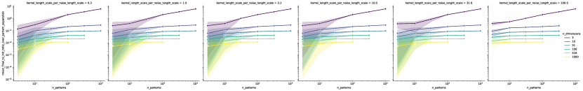
Figure 8: KDE as associative memory: memory capacity limits. We sample $N$ patterns on a $D$-dimensional hypersphere of radius $M=2\sqrt{D-1}$, which we use to define our energy landscape. We then initialize 100 particles perturbed from the positions of each pattern, and let them evolve under the energy function. We calculate the mean ratio of the distance between particles and their corresponding patterns after undergoing dynamics, divided by this distance at initialization. We then normalize this ratio by the average distance of patterns. The smaller this ratio is, the closer the particles have converged to their corresponding patterns. We see that increasing the number of patterns results in poorer retrieval, while increasing the number of dimensions results in better retrieval.

References

- Abu-Mostafa & Jacques (1985) Abu-Mostafa, Y. and Jacques, J. S. Information capacity of the hopfield model. IEEE Transactions on Information Theory, 31(4):461–464, 1985.
- Aldous et al. (1985) Aldous, D. J., Ibragimov, I. A., Jacod, J., and Aldous, D. J. Exchangeability and related topics. Springer, 1985.
- Ambrogioni (2023) Ambrogioni, L. In search of dispersed memories: Generative diffusion models are associative memory networks. arXiv preprint arXiv:2309.17290, 2023.
- Annabi et al. (2022) Annabi, L., Pitti, A., and Quoy, M. On the relationship between variational inference and auto-associative memory. Advances in Neural Information Processing Systems, 35:37497–37509, 2022.
- Antoniak (1974) Antoniak, C. E. Mixtures of dirichlet processes with applications to bayesian nonparametric problems. The annals of statistics, pp. 1152–1174, 1974.
- Ba et al. (2016) Ba, J. L., Kiros, J. R., and Hinton, G. E. Layer normalization. arXiv preprint arXiv:1607.06450, 2016.
- Baevski & Auli (2018) Baevski, A. and Auli, M. Adaptive input representations for neural language modeling. arXiv preprint arXiv:1809.10853, 2018.
- Barra et al. (2018) Barra, A., Beccaria, M., and Fachechi, A. A new mechanical approach to handle generalized hopfield neural networks. Neural Networks, 106:205–222, 2018.
- Bischof et al. (1999) Bischof, H., Leonardis, A., and Selb, A. Mdl principle for robust vector quantisation. Pattern Analysis & Applications, 2:59–72, 1999.
- Bishop & Nasrabadi (2006) Bishop, C. M. and Nasrabadi, N. M. Pattern recognition and machine learning, volume 4. Springer, 2006.
- Blackwell & MacQueen (1973) Blackwell, D. and MacQueen, J. B. Ferguson distributions via pólya urn schemes. The annals of statistics, 1(2):353–355, 1973.
- Bricken & Pehlevan (2021) Bricken, T. and Pehlevan, C. Attention approximates sparse distributed memory. Advances in Neural Information Processing Systems, 34:15301–15315, 2021.
- Brown et al. (2020) Brown, T., Mann, B., Ryder, N., Subbiah, M., Kaplan, J. D., Dhariwal, P., Neelakantan, A., Shyam, P., Sastry, G., Askell, A., et al. Language models are few-shot learners. Advances in neural information processing systems, 33:1877–1901, 2020.
- Chan et al. (2022) Chan, S., Santoro, A., Lampinen, A., Wang, J., Singh, A., Richemond, P., McClelland, J., and Hill, F. Data distributional properties drive emergent in-context learning in transformers. Advances in Neural Information Processing Systems, 35:18878–18891, 2022.
- Chatterjee et al. (2022) Chatterjee, S., Romero, O., and Pequito, S. Analysis of a generalised expectation–maximisation algorithm for gaussian mixture models: a control systems perspective. International Journal of Control, 95(10):2734–2742, 2022.
- Chaudhuri & Fiete (2019) Chaudhuri, R. and Fiete, I. Bipartite expander hopfield networks as self-decoding high-capacity error correcting codes. Advances in neural information processing systems, 32, 2019.
- Child et al. (2019) Child, R., Gray, S., Radford, A., and Sutskever, I. Generating long sequences with sparse transformers. arXiv preprint arXiv:1904.10509, 2019.
- Crisanti et al. (1986) Crisanti, A., Amit, D. J., and Gutfreund, H. Saturation level of the hopfield model for neural network. Europhysics Letters, 2(4):337, 1986.
- Dehghani et al. (2023) Dehghani, M., Djolonga, J., Mustafa, B., Padlewski, P., Heek, J., Gilmer, J., Steiner, A. P., Caron, M., Geirhos, R., Alabdulmohsin, I., et al. Scaling vision transformers to 22 billion parameters. In International Conference on Machine Learning, pp. 7480–7512. PMLR, 2023.
- Demircigil et al. (2017) Demircigil, M., Heusel, J., Löwe, M., Upgang, S., and Vermet, F. On a model of associative memory with huge storage capacity. Journal of Statistical Physics, 168:288–299, 2017.
- Dempster et al. (1977) Dempster, A. P., Laird, N. M., and Rubin, D. B. Maximum likelihood from incomplete data via the em algorithm. Journal of the royal statistical society: series B (methodological), 39(1):1–22, 1977.
- Du & Mordatch (2019) Du, Y. and Mordatch, I. Implicit generation and modeling with energy based models. Advances in Neural Information Processing Systems, 32, 2019.
- Du et al. (2020a) Du, Y., Li, S., and Mordatch, I. Compositional visual generation with energy based models. Advances in Neural Information Processing Systems, 33:6637–6647, 2020a.
- Du et al. (2020b) Du, Y., Li, S., Tenenbaum, J., and Mordatch, I. Improved contrastive divergence training of energy based models. arXiv preprint arXiv:2012.01316, 2020b.
- Du et al. (2021) Du, Y., Li, S., Sharma, Y., Tenenbaum, J., and Mordatch, I. Unsupervised learning of compositional energy concepts. Advances in Neural Information Processing Systems, 34:15608–15620, 2021.
- Epanechnikov (1969) Epanechnikov, V. A. Non-parametric estimation of a multivariate probability density. Theory of Probability & Its Applications, 14(1):153–158, 1969.
- Fisher (1953) Fisher, R. A. Dispersion on a sphere. Proceedings of the Royal Society of London. Series A. Mathematical and Physical Sciences, 217(1130):295–305, 1953.
- Folli et al. (2017) Folli, V., Leonetti, M., and Ruocco, G. On the maximum storage capacity of the hopfield model. Frontiers in computational neuroscience, 10:144, 2017.
- Fuentes-García et al. (2019) Fuentes-García, R., Mena, R. H., and Walker, S. G. Modal posterior clustering motivated by hopfield’s network. Computational Statistics & Data Analysis, 137:92–100, 2019.
- Gardner (1988) Gardner, E. The space of interactions in neural network models. Journal of physics A: Mathematical and general, 21(1):257, 1988.
- Garg et al. (2022) Garg, S., Tsipras, D., Liang, P. S., and Valiant, G. What can transformers learn in-context? a case study of simple function classes. Advances in Neural Information Processing Systems, 35:30583–30598, 2022.
- Hamerly & Elkan (2003) Hamerly, G. and Elkan, C. Learning the k in k-means. Advances in neural information processing systems, 16, 2003.
- Hastie et al. (2009) Hastie, T., Tibshirani, R., Friedman, J. H., and Friedman, J. H. The elements of statistical learning: data mining, inference, and prediction, volume 2. Springer, 2009.
- Hendrycks & Gimpel (2016) Hendrycks, D. and Gimpel, K. Gaussian error linear units (gelus). arXiv preprint arXiv:1606.08415, 2016.
- Hinton (2002) Hinton, G. E. Training products of experts by minimizing contrastive divergence. Neural computation, 14(8):1771–1800, 2002.
- Hoover et al. (2023a) Hoover, B., Liang, Y., Pham, B., Panda, R., Strobelt, H., Chau, D. H., Zaki, M. J., and Krotov, D. Energy transformer. 2023a.
- Hoover et al. (2023b) Hoover, B., Strobelt, H., Krotov, D., Hoffman, J., Kira, Z., and Chau, D. H. Memory in plain sight: A survey of the uncanny resemblances between diffusion models and associative memories. arXiv preprint arXiv:2309.16750, 2023b.
- Hopfield (1982) Hopfield, J. J. Neural networks and physical systems with emergent collective computational abilities. Proceedings of the national academy of sciences, 79(8):2554–2558, 1982.
- Hopfield (1984) Hopfield, J. J. Neurons with graded response have collective computational properties like those of two-state neurons. Proceedings of the national academy of sciences, 81(10):3088–3092, 1984.
- Hopfield & Tank (1986) Hopfield, J. J. and Tank, D. W. Computing with neural circuits: A model. Science, 233(4764):625–633, 1986.
- Josselyn & Tonegawa (2020) Josselyn, S. A. and Tonegawa, S. Memory engrams: Recalling the past and imagining the future. Science, 367(6473):eaaw4325, 2020.
- Jung et al. (2023) Jung, J. H., Wang, Y., Mocle, A. J., Zhang, T., Köhler, S., Frankland, P. W., and Josselyn, S. A. Examining the engram encoding specificity hypothesis in mice. Neuron, 111(11):1830–1845, 2023.
- Krotov & Hopfield (2020) Krotov, D. and Hopfield, J. Large associative memory problem in neurobiology and machine learning. arXiv preprint arXiv:2008.06996, 2020.
- Krotov & Hopfield (2016) Krotov, D. and Hopfield, J. J. Dense associative memory for pattern recognition. Advances in neural information processing systems, 29, 2016.
- Kulis & Jordan (2012) Kulis, B. and Jordan, M. I. Revisiting k-means: new algorithms via bayesian nonparametrics. In Proceedings of the 29th International Coference on International Conference on Machine Learning, pp. 1131–1138, 2012.
- Lau et al. (2020) Lau, J. M., Rashid, A. J., Jacob, A. D., Frankland, P. W., Schacter, D. L., and Josselyn, S. A. The role of neuronal excitability, allocation to an engram and memory linking in the behavioral generation of a false memory in mice. Neurobiology of learning and memory, 174:107284, 2020.
- Lisman et al. (2018) Lisman, J., Cooper, K., Sehgal, M., and Silva, A. J. Memory formation depends on both synapse-specific modifications of synaptic strength and cell-specific increases in excitability. Nature neuroscience, 21(3):309–314, 2018.
- Lucibello & Mézard (2023) Lucibello, C. and Mézard, M. The exponential capacity of dense associative memories. arXiv preprint arXiv:2304.14964, 2023.
- McEliece et al. (1987) McEliece, R., Posner, E., Rodemich, E., and Venkatesh, S. The capacity of the hopfield associative memory. IEEE transactions on Information Theory, 33(4):461–482, 1987.
- Millidge et al. (2022) Millidge, B., Salvatori, T., Song, Y., Lukasiewicz, T., and Bogacz, R. Universal hopfield networks: A general framework for single-shot associative memory models. In International Conference on Machine Learning, pp. 15561–15583. PMLR, 2022.
- Mordatch (2018) Mordatch, I. Concept learning with energy-based models. arXiv preprint arXiv:1811.02486, 2018.
- Neal & Hinton (1998) Neal, R. M. and Hinton, G. E. A view of the em algorithm that justifies incremental, sparse, and other variants. In Learning in graphical models, pp. 355–368. Springer, 1998.
- Nijkamp et al. (2020) Nijkamp, E., Hill, M., Han, T., Zhu, S.-C., and Wu, Y. N. On the anatomy of mcmc-based maximum likelihood learning of energy-based models. In Proceedings of the AAAI Conference on Artificial Intelligence, volume 34, pp. 5272–5280, 2020.
- Park et al. (2016) Park, S., Kramer, E. E., Mercaldo, V., Rashid, A. J., Insel, N., Frankland, P. W., and Josselyn, S. A. Neuronal allocation to a hippocampal engram. Neuropsychopharmacology, 41(13):2987–2993, 2016.
- Parzen (1962) Parzen, E. On estimation of a probability density function and mode. The annals of mathematical statistics, 33(3):1065–1076, 1962.
- Pelleg et al. (2000) Pelleg, D., Moore, A. W., et al. X-means: Extending k-means with efficient estimation of the number of clusters. In Icml, volume 1, pp. 727–734, 2000.
- Pignatelli et al. (2019) Pignatelli, M., Ryan, T. J., Roy, D. S., Lovett, C., Smith, L. M., Muralidhar, S., and Tonegawa, S. Engram cell excitability state determines the efficacy of memory retrieval. Neuron, 101(2):274–284, 2019.
- Pitman (2006) Pitman, J. Combinatorial stochastic processes: Ecole d’eté de probabilités de saint-flour xxxii-2002. Springer, 2006.
- Radford et al. (2018) Radford, A., Narasimhan, K., Salimans, T., Sutskever, I., et al. Improving language understanding by generative pre-training. 2018.
- Radford et al. (2019) Radford, A., Wu, J., Child, R., Luan, D., Amodei, D., Sutskever, I., et al. Language models are unsupervised multitask learners. OpenAI blog, 1(8):9, 2019.
- Radhakrishnan et al. (2018) Radhakrishnan, A., Yang, K., Belkin, M., and Uhler, C. Memorization in overparameterized autoencoders. arXiv preprint arXiv:1810.10333, 2018.
- Radhakrishnan et al. (2020) Radhakrishnan, A., Belkin, M., and Uhler, C. Overparameterized neural networks implement associative memory. Proceedings of the National Academy of Sciences, 117(44):27162–27170, 2020.
- Ramsauer et al. (2020) Ramsauer, H., Schäfl, B., Lehner, J., Seidl, P., Widrich, M., Adler, T., Gruber, L., Holzleitner, M., Pavlović, M., Sandve, G. K., et al. Hopfield networks is all you need. arXiv preprint arXiv:2008.02217, 2020.
- Rashid et al. (2016) Rashid, A. J., Yan, C., Mercaldo, V., Hsiang, H.-L., Park, S., Cole, C. J., De Cristofaro, A., Yu, J., Ramakrishnan, C., Lee, S. Y., et al. Competition between engrams influences fear memory formation and recall. Science, 353(6297):383–387, 2016.
- Romero et al. (2019) Romero, O., Chatterjee, S., and Pequito, S. Convergence of the expectation-maximization algorithm through discrete-time lyapunov stability theory. In 2019 American Control Conference (ACC), pp. 163–168. IEEE, 2019.
- Rosenblatt (1956) Rosenblatt, M. Remarks on some nonparametric estimates of a density function. The annals of mathematical statistics, pp. 832–837, 1956.
- Rousseeuw (1987) Rousseeuw, P. J. Silhouettes: a graphical aid to the interpretation and validation of cluster analysis. Journal of computational and applied mathematics, 20:53–65, 1987.
- Rumelhart et al. (1986) Rumelhart, D. E., Hinton, G. E., and Williams, R. J. Learning representations by back-propagating errors. Nature, 323(6088):533–536, 1986.
- Saha et al. (2023) Saha, B., Krotov, D., Zaki, M. J., and Ram, P. End-to-end differentiable clustering with associative memories. arXiv preprint arXiv:2306.03209, 2023.
- Salakhutdinov et al. (2003) Salakhutdinov, R., Roweis, S. T., and Ghahramani, Z. Optimization with em and expectation-conjugate-gradient. In Proceedings of the 20th International Conference on Machine Learning (ICML-03), pp. 672–679, 2003.
- Schaeffer et al. (2023) Schaeffer, R., Khona, M., Zahedi, N., Fiete, I. R., Gromov, A., and Koyejo, S. Associative memory under the probabilistic lens: Improved transformers & dynamic memory creation. In Associative Memory & Hopfield Networks in 2023, 2023.
- Sharma et al. (2022) Sharma, S., Chandra, S., and Fiete, I. Content addressable memory without catastrophic forgetting by heteroassociation with a fixed scaffold. In International Conference on Machine Learning, pp. 19658–19682. PMLR, 2022.
- Sheather & Jones (1991) Sheather, S. J. and Jones, M. C. A reliable data-based bandwidth selection method for kernel density estimation. Journal of the Royal Statistical Society: Series B (Methodological), 53(3):683–690, 1991.
- Sugar & James (2003) Sugar, C. A. and James, G. M. Finding the number of clusters in a dataset: An information-theoretic approach. Journal of the American Statistical Association, 98(463):750–763, 2003.
- Tanaka & Edwards (1980) Tanaka, F. and Edwards, S. Analytic theory of the ground state properties of a spin glass. i. ising spin glass. Journal of Physics F: Metal Physics, 10(12):2769, 1980.
- Teh et al. (2010) Teh, Y. W. et al. Dirichlet process. Encyclopedia of machine learning, 1063:280–287, 2010.
- Thorndike (1953) Thorndike, R. L. Who belongs in the family? Psychometrika, 18(4):267–276, 1953.
- Tibshirani et al. (2001) Tibshirani, R., Walther, G., and Hastie, T. Estimating the number of clusters in a data set via the gap statistic. Journal of the Royal Statistical Society: Series B (Statistical Methodology), 63(2):411–423, 2001.
- Torres et al. (2002) Torres, J. J., Pantic, L., and Kappen, H. J. Storage capacity of attractor neural networks with depressing synapses. Physical Review E, 66(6):061910, 2002.
- Vaswani et al. (2017) Vaswani, A., Shazeer, N., Parmar, N., Uszkoreit, J., Jones, L., Gomez, A. N., Kaiser, Ł., and Polosukhin, I. Attention is all you need. Advances in neural information processing systems, 30, 2017.
- Wand & Jones (1994) Wand, M. P. and Jones, M. C. Kernel smoothing. CRC press, 1994.
- Wang et al. (2019) Wang, Q., Li, B., Xiao, T., Zhu, J., Li, C., Wong, D. F., and Chao, L. S. Learning deep transformer models for machine translation. arXiv preprint arXiv:1906.01787, 2019.
- Wortsman et al. (2023) Wortsman, M., Liu, P. J., Xiao, L., Everett, K., Alemi, A., Adlam, B., Co-Reyes, J. D., Gur, I., Kumar, A., Novak, R., et al. Small-scale proxies for large-scale transformer training instabilities. arXiv preprint arXiv:2309.14322, 2023.
- Xiong et al. (2020) Xiong, R., Yang, Y., He, D., Zheng, K., Zheng, S., Xing, C., Zhang, H., Lan, Y., Wang, L., and Liu, T. On layer normalization in the transformer architecture. In International Conference on Machine Learning, pp. 10524–10533. PMLR, 2020.
- Xu & Jordan (1996) Xu, L. and Jordan, M. I. On convergence properties of the em algorithm for gaussian mixtures. Neural computation, 8(1):129–151, 1996.
- Yiu et al. (2014) Yiu, A. P., Mercaldo, V., Yan, C., Richards, B., Rashid, A. J., Hsiang, H.-L. L., Pressey, J., Mahadevan, V., Tran, M. M., Kushner, S. A., et al. Neurons are recruited to a memory trace based on relative neuronal excitability immediately before training. Neuron, 83(3):722–735, 2014.
- Zhai et al. (2023) Zhai, S., Likhomanenko, T., Littwin, E., Busbridge, D., Ramapuram, J., Zhang, Y., Gu, J., and Susskind, J. M. Stabilizing transformer training by preventing attention entropy collapse. In International Conference on Machine Learning, pp. 40770–40803. PMLR, 2023.
- Zhang & Sennrich (2019) Zhang, B. and Sennrich, R. Root mean square layer normalization. Advances in Neural Information Processing Systems, 32, 2019.