Thermodynamically Stable Knots in Semiflexible Polymers

Abstract

Semiflexible polymers are widely used as a paradigm for understanding structural phases in biomolecules including folding of proteins. Here, we compare bead-spring and bead-stick variants of coarse-grained semiflexible polymer models that cover the whole range from flexible to stiff by conducting extensive replica-exchange Monte Carlo computer simulations. In the data analysis we focus on knotted conformations whose stability is shown to depend on the ratio $r_{b}/r_{\rm min}$ with $r_{b}$ denoting the equilibrium bond length and $r_{\rm min}$ the distance of the strongest nonbonded interactions. For both models, our results provide evidence that at low temperatures for $r_{b}/r_{\rm min}$ outside a small range around unity one always encounters knots as generic stable phases along with the usual frozen and bent-like structures. By varying the bending stiffness, we observe rather strong first-order-like structural transitions between the coexisting phases characterized by these geometrically different motifs. Through analyses of the energy distributions close to the transition point, we present exploratory estimates of the free-energy barriers between the coexisting phases.

1 Introduction

Computer simulation studies of atomistic macromolecular systems are often limited by the accessible time scales. One therefore often considers less expensive coarse-grained models that are sufficient for understanding the generic features of macromolecules muller2002coarse . This approach can be classified into bead-spring and bead-stick polymer models. In addition to excluded volume effects and interactions among the monomers or beads, for semiflexible biopolymers one also has to take into account bending stiffness of the chain kratky1949 . With this motivation in mind, Seaton et al. seaton2013flexible explored different phases (coiled, collapsed, frozen, bent, hairpin, and toroidal conformations) of a bead-spring model by tuning the bending stiffness $\kappa$. Similar phases show up in a bead-stick model marenz2016knots where in addition one observes at low temperatures $T$ also phases dominated by thermodynamically stable knotted structures. For a sketch of the generic ($T,\kappa$) phase diagram, see Fig. 1. In Ref. marenz2016knots it has been conjectured that the propensity for forming knots may depend on the ratio of the equilibrium bond length $r_{b}$ to the distance $r_{\rm{min}}$ where the nonbonded interaction potential is at its minimum, i.e., the attractive interaction is strongest.

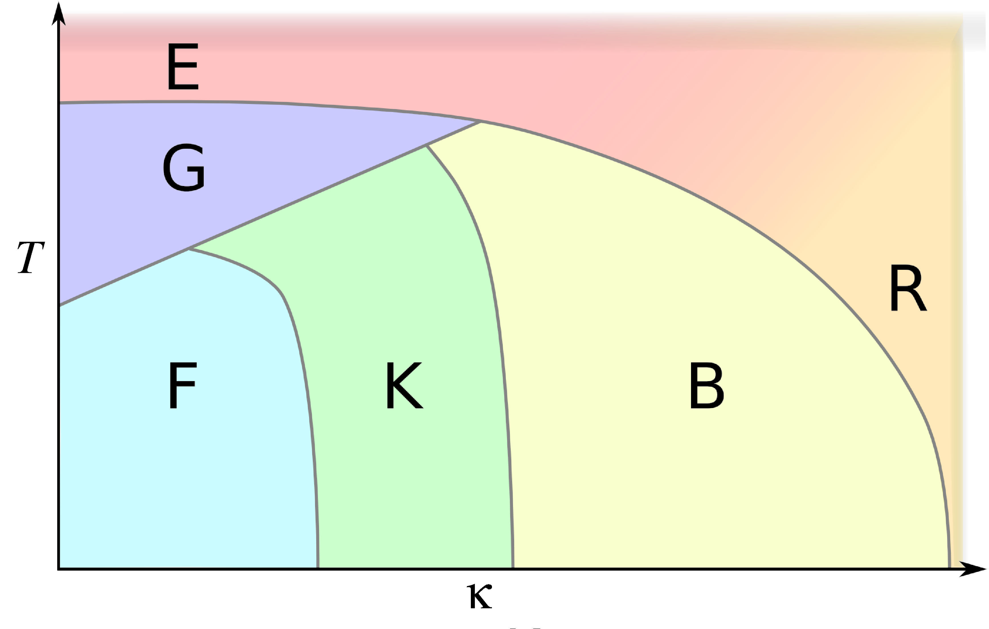
Figure 1: Generic phase diagram for a semiflexible polymer in the ($T,\kappa$) plane. The labels stand short for E: Extended coils, R: Rods G: Globules, F: Frozen, K: Stable knot phase, B: Bent.

To shed more light onto the puzzle why knots apparently appear only in one of the two models, we recently performed extensive comparative Monte Carlo simulations macromolecules21 . Our numerical results provide evidence that for both model variants, in certain ranges of bending stiffness, knotted structures are always observed when $r_{b}/r_{\rm{min}}$ is away from a small region around unity. Analytically, this can be understood by the competition of the nonbonded interaction and bending energy when minimizing the total energy.

2 Models and Simulation

In both model variants, spherical beads with diameter $\sigma$ are considered as the monomers and the nonbonded interaction energy among them is taken for a polymer chain of length $N$ as

$$E_{\rm nb}(r_{ij})=\sum_{i=1}^{N-2}\sum_{j=i+2}^{N}\left[E_{\rm{LJ}}({\rm{min}}\{r_{ij},r_{c}\})-E_{\rm{LJ}}(r_{c})\right]$$ (1)

with the Lennard-Jones (LJ) potential

$$E_{\rm{LJ}}(r_{ij})=4\epsilon\left[\left(\frac{\sigma}{r_{ij}}\right)^{12}-\left(\frac{\sigma}{r_{ij}}\right)^{6}\right]$$ (2)

where $r_{ij}$ denotes the distance between the beads. The parameters $\sigma$ and $\epsilon=1$ set the length and energy scales, respectively. Both $E_{\rm nb}$ and $E_{\rm LJ}$ have a minimum at $r_{\rm min}=2^{1/6}\sigma$ with $E_{\rm LJ,min}=-\epsilon$. To be consistent with Ref. seaton2013flexible , for the bead-spring model we employ a cutoff distance $r_{c}=2.5\sigma$ and set $\sigma=2^{-1/6}$, implying $r_{\rm min}=1$, whereas following our earlier work marenz2016knots , for the bead-stick model we do not apply any cutoff distance and set $\sigma=1$ such that $r_{\rm min}=2^{1/6}$. To model the bonds by springs between successive beads in the bead-spring model, we use the standard finitely extensible non-linear elastic (FENE) potential milchev1993off ; milchev2001formation

$$E_{\rm FENE}=-\frac{K}{2}R^{2}\sum_{i=1}^{N-1}\ln\left[1-\left(\frac{r_{ii+1}-r_{b}}{R}\right)^{2}\right]$$ (3)

with $r_{b}$ denoting the equilibrium bond length where $E_{\rm{FENE}}$ is minimal, $R=0.3$, and $K=40$. The rigid bonds or sticks in the bead-stick model are assumed to have a fixed bond length $r_{b}$, i.e., here formally $E_{\rm FENE}\equiv 0$. The sum of nonbonded and bonded interactions (apart from bending stiffness) is denoted by $E_{0}=E_{\rm nb}+E_{\rm FENE}$

The bending stiffness is introduced via the well-known discretized worm-like chain cosine potential

$$E_{\rm{bend}}\equiv\kappa E_{1}=\kappa\sum_{i=1}^{N-2}(1-\cos\theta_{i})$$ (4)

where $\theta_{i}$ is the angle between consecutive bonds and the model parameter $\kappa$ controls the effective bending stiffness of the polymer. The total energy of the semiflexible polymer is then $E=E_{0}+E_{\rm bend}=E_{0}+\kappa E_{1}$.

While this model still looks rather simple, its simulation demands application of relatively complex Monte Carlo (MC) methods janke2018macromolecule . Previously marenz2016knots we have used a parallelized version of the multicanonical algorithm berg1991multicanonical ; zierenberg2013scaling ; janke2016SM along with replica exchange (RE) (also known as parallel tempering) hukushima1996exchange and validated the results with the two-dimensional replica exchange method (2D-RE). In Ref. macromolecules21 we restricted ourselves to the 2D-RE algorithm. The set of attempted MC updates included the usual crank-shaft, spherical-rotation, and pivot moves Austin2018 .

The definition of knots in an open polymer chain requires some care. Mathematically, knots can be defined only for closed curves kauffman1991 . One therefore has first to close an open polymer chain virtually for which several rules are possible. We employed the specific closure prescription as discussed in Refs. virnau2005knots ; virnau2010 ; marenz2016knots ; janke2016stable and depicted in Fig. 2.

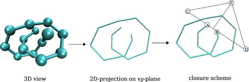
Figure 2: Closure scheme for an open polymer conformation in three-dimensional space (3D view) applied to its two-dimensional projection onto one plane of a Cartesian coordinate system (2D projection on $xy$-plane). Taken from Ref. macromolecules21 .

The type of a knot is denoted by $C_{n}$ where the integer $C$ counts the minimum number of crossings and the subscript $n$ distinguishes knots that differ topologically kauffman1991 . For example, the sketch in Fig. 2 shows the trefoil knot 3₁. In a numerical analysis this classification can be determined by computing topological invariants such as the Alexander polynomial $\Delta(t)$ kauffman1991 . More precisely we actually computed the knot parameter

$$D=\Delta_{p}(-1.1)$$ (5)

where $\Delta_{p}(t)=\lvert\Delta(t)\times\Delta(1/t)\rvert$ removes undesired prefactors and the choice of the argument $t=-1.1$ is justified empirically virnau2005knots ; virnau2010 . It is well known that even though for complicated knots the Alexander polynomial and hence also $D$ is not unique [e.g., $D(5_{1})=D(10_{132})$] kauffman1991 , all the simple knots relevant in this work can be distinguished by the parameter (5); see Table 1 of Ref. macromolecules21 . For instance, $D=1$ for an unknotted chain and $D\approx 9.05463$, 25.09099, 25.45745, or 9.72667 for a chain with a 3₁, 4₁, 5₁, or 8₁₉ knot. For a schematic illustration see Fig. 3.

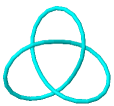
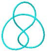
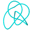
Figure 3: Sketch of the knot type 3₁ characterizing the stable knot phase K3₁ for semiflexible polymers of length $N=14$ and the knot types 4₁, 5₁, and 8₁₉ occurring for $N=28$.

3 Results

In the analysis of our Monte Carlo data, while mainly focusing on the behavior of the knot parameter, we have constructed in Ref. macromolecules21 the entire phase diagrams of the bead-spring and bead-stick models in the ($T,\kappa$) plane for several ratios $r_{b}/r_{\rm min}$. To this end we performed elaborate simulations at many $T$ and $\kappa$ points for chain length $N=14$ (and less extensively also for $N=28$) and determined beside the average knot parameter $\langle D\rangle$ also several other observables such as the average squared radius of gyration $\langle R^{2}_{g}\rangle$, its temperature derivative, the average energies $\langle E_{0}\rangle$, $\langle E_{1}\rangle$, and $\langle E\rangle=\langle E_{0}\rangle+\kappa\langle E_{1}\rangle$, as well as the specific heat $C_{v}=\mathrm{d}\langle E\rangle/\mathrm{d}T=(1/T^{2})(\langle E^{2}\rangle-\langle E\rangle^{2})$. By means of the weighted histogram analysis method (WHAM), this information was finally combined to arrive at a quantitative version of the generic phase diagram sketched in Fig. 1.

In Fig. 4 we focus only on the average knot parameter $\langle D\rangle$ which is shown in surface plots for the bead-spring (left) and bead-stick (right) models with chain length $N=14$ for five different values of the ratio $r_{b}/r_{\rm{min}}$ ($=2^{-1/6}\approx 0.891,1.000,2^{1/6}\approx 1.122,2^{2/6}\approx 1.260$, and $2^{4/6}\approx 1.587$). The dark red color indicates regions in the phase diagram that are populated by conformations forming a trefoil knot 3₁ with $D\approx 9.05463$, whereas yellow color signals unknotted (e.g., bent or extended) conformations. The blue boundary layer results from phase coexistence of a finite system [$D\approx(9.05+1)/2\approx 5)$], for more details see below.

For the smallest ratio $r_{b}/r_{\rm{min}}=2^{-1/6}\approx 0.891$ the knot phase is rather pronounced and seems to be a bit wider for the bead-spring than the bead-stick model. In both models, it significantly shrinks for $r_{b}/r_{\rm{min}}=1$, and for $r_{b}/r_{\rm{min}}=2^{1/6}\approx 1.122$ it basically has disappeared. By estimating the energies needed for forming a 3₁ knot and a bent conformation (with three segments), respectively, one concludes that bent conformations are more favorable in this case (the temperature is so low that entropic contributions can be safely neglected) macromolecules21 .

For larger ratios, the K3₁ knot phase reoccurs at smaller values of $\kappa$. The main difference is that here the knot geometry is flat while for $r_{b}<r_{\rm min}$ it is spherical macromolecules21 . The light red (or orange) region for $r_{b}/r_{\rm min}=1.587$ at small $\kappa$ extending to relatively high $T$ signals a mixed phase of 4₁ knots and unknotted conformations encoded by $D\approx(25.09+1)/2\approx 13$ (it does not correspond to the 8₁₉ knot with $D\approx 9.72667$ since the $N=14$ chain is too short to accommodate a knot with 8 crossings).

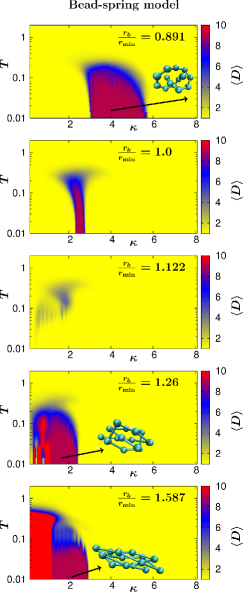
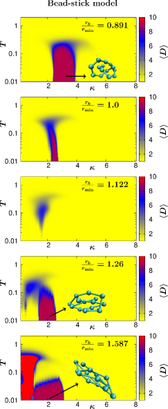
Figure 4: Phase diagram for a semiflexible polymer of length $N=14$ in the ($T,\kappa$) plane with the average knot parameter $\langle D\rangle$ as order parameter and several choices of the ratio $r_{b}/r_{\rm{min}}$ using a bead-spring (left) and bead-stick (right) model. The snapshots show typical polymer conformations in the phase characterized by a stable trefoil knot $3_{1}$. Taken from Ref. macromolecules21 .

As already observed in Ref. marenz2016knots and mentioned above, most of the low-temperature (pseudo) phase transitions exhibit a fairly strong first-order signal which is caused by the pronounced coexistence of different conformational motifs (e.g., bent and knotted). This explains why the computer simulations are so demanding and require the application of quite elaborate sophisticated methods janke_rugged . In the following we shall mainly focus on the blue colored region of transitions between the bent (B) and knot (K) phase when $\kappa$ is varied at low temperature, cf. Figs. 1 and 4. For $N=14$ and 28, the specific bent phase is of type D3 in both cases, featuring bent conformations with 3 segments, and the knot phases are characterized by 3₁ and 5₁ knots, respectively. Note that for larger $N$, the phase diagram is much richer and the picture becomes more complicated. For instance, with $N=42$ we observed transitions between the bent phase of type D6 and the K7₁ knot phase at low temperature respectively with the K8₅ knot phase at very low temperature marenz-wj-tobe .

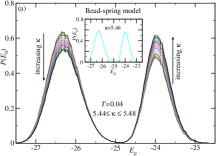
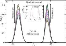
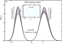
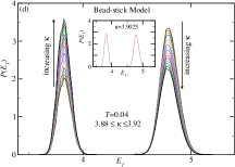
Figure 5: Probability distributions $P(E_{0})$ and $P(E_{1})$ of the two contributions $E_{0}=E_{\rm nb}+E_{\rm FENE}$ and $E_{1}=E_{\rm bend}/\kappa$ to the total energy $E=E_{0}+\kappa E_{1}$ in dependence of $\kappa$ close to the transition between the K3₁ knot phase and the bent phase of type D3 at $T=0.04$. The left panels (a), (c) show our results for the bead-spring model and the right panels (b), (d) those for the bead-stick model (where $E_{\rm FENE}\equiv 0$) with $r_{b}/r_{\rm min}=0.891$ and chain length $N=14$. The insets concentrate on the phase-transition point $\kappa_{t}$, defined from the distribution for which the two peaks have equal height. Computing the ratio of maximum to minimum and taking the logarithm yields estimates of the free-energy barriers at the transition (cf. Table 3).

These structural transitions turned out to be very intriguing since they do not carry any obvious first-order signal in the total energy $E=E_{0}+\kappa E_{1}$; rather, the distribution $P(E)$ looks apparently single-peaked which is the typical signature of a smooth second-order transition. Only when looking at the two-dimensional distribution $P(E_{0},E_{1})$ a bimodal structure becomes clearly visible marenz2016knots which is typical for a first-order-like transition. The double-peak structure is also shared by the individual one-dimensional distributions $P(E_{0})$ and $P(E_{1})$ separately. This is illustrated in Fig. 5 for the $N=14$ chain with $r_{b}/r_{\rm min}=0.891$ which shows for $T=0.04$ how the double peak varies as the bending stiffness $\kappa$ changes across the transition point $\kappa_{t}$. In $P(E_{0})$ the left peak corresponds to the knot phase and the right peak to the bent phase, whereas for $P(E_{1})$ this is just reversed. The insets highlight the situation where both peaks are of equal height which is usually used as a criterion for locating the phase-transition point wj_prb93 ; janke_1st-order-review .

The ratio of maximum to minimum of the equal-height probability distribution determines the strength or “hardness” of a first-order transition wj_prb93 ; janke_1st-order-review , which is directly related to the corresponding free-energy barrier per monomer $\Delta f=T\ln\left(P_{\rm max}/P_{\rm min}\right)/N$ janke_2017 ; zierenberg_natcomm . The quantitative results for the two examples in Fig. 5 are compiled in Table 3. The much larger ratios for the bead-stick model indicate that with fixed bonds the K3₁ knot phase is considerably more stable against forming bent conformations of D$3$ type than with flexible springs. This is intuitively expected since the deformation of conformational motifs is easier with flexible springs than with stiff bonds.

The results presented here in Fig. 5 and Table 3 are only of explorative nature. We are currently investigating the shapes of the energy distributions and the associated free-energy barriers also at several other structural transitions and in particular for larger chain lengths $N$. This is a rather ambitious endeavor which requires fairly long simulation and analysis times, and hence further more extensive results will be reported elsewhere sm_sp_wj-tobe .

Table 1: Parameters of the double-peak distributions $P(E_{0})$ and $P(E_{1})$ of a semiflexible polymer with $N=14$ beads shown in the insets of Fig. 5 at the transitions D3 $\leftrightarrow$ K3₁ for $T=0.04$ at $\kappa_{t}$. “ratio” stands short for the ratio $P_{\rm max}/P_{\rm min}$.

model	$\kappa_{t}$	$P_{\rm max}(E_{0})$	$P_{\rm min}(E_{0})$	ratio	$P_{\rm max}(E_{1})$	$P_{\rm min}(E_{1})$	ratio
bead-spring	5.46	0.58	0.003	193	3.61	0.01	361
bead-stick	3.9025	0.67	$4.26\times 10^{-5}$	15 728	2.88	$4.02\times 10^{-4}$	7 164

4 Discussion

As we have seen in Figs. 4 and 5, semiflexible bead-spring and bead-stick models behave qualitatively very similarly and both exhibit the same generic phase diagram depicted in Fig. 1. So, why did Seaton et al. seaton2013flexible not identify knots in their seminal study of a bead-spring model? There are several related reasons:

1. In this first study of the entire phase diagram for a semiflexible polymer, they focused on bent, toroidal, etc. motifs, but did not actively search for knots.

2. The parameterization employed in Ref. seaton2013flexible realizes the ratio $r_{b}/r_{\rm min}=1$ where only a very small region of the phase diagram is populated with knots. Moreover, knots predominantly occur at very low temperatures below the lower limit of their study.

3. The parameterization of the bead-spring model in Ref. seaton2013flexible is a bit uncommon. We have shown that it corresponds in good approximation to our bead-spring model, albeit with an extremely large spring constant of $K=297.5$ macromolecules21 . With additional simulations we have explicitly verified macromolecules21 that for such a large spring constant, as expected, the bead-spring model is basically indistinguishable from the bead-stick model.

5 Conclusions

Our extensive two-dimensional replica-exchange Monte Carlo simulations of bead-stick and bead-spring homopolymer models confirm the theoretical expectation that the existence of stable knotted phases depends on the ratio $r_{b}/r_{\rm min}$ between the equilibrium bond length $r_{b}$ and the distance $r_{\rm min}$ of the strongest attraction of nonbonded beads. By simple energy arguments one can read off that for $r_{b}/r_{\rm min}\approx 1$ the alternative bent motifs are more favorable than knotted structures. This is compatible with our study of a semiflexible polymer adsorbed on a flat surface where with the choice $r_{b}/r_{\rm min}=1$ (and not very low temperatures $T\geq 0.1$) we did not observe knots austin2017interplay . This is probably also the main explanation why no knots have been reported in the simulation study of Seaton et al. seaton2013flexible .

The transitions between the various structural motifs at low temperatures are first-order-like with pronounced phase coexistence at the transition point. In the energy distributions, this is reflected by a double-peak structure which we exploit for estimating the free-energy barriers. The results of the exploratory study described here are promising and a more detailed investigation will be reported elsewhere sm_sp_wj-tobe .

- (1) Müller-Plathe, F.: Coarse-graining in polymer simulation: From the atomistic to the mesoscopic scale and back. Chem. Phys. Chem. 3, 754–769 (2002)
- (2) Kratky, O., Porod, G.: Röntgenuntersuchung gelöster Fadenmoleküle. Rec. Trav. Chim. Pays-Bas 68, 1106–1122 (1949)
- (3) Seaton, D., Schnabel, S., Landau, D., Bachmann, M.: From flexible to stiff: Systematic analysis of structural phases for single semiflexible polymers. Phys. Rev. Lett. 110, 028,103 (2013)
- (4) Marenz, M., Janke, W.: Knots as a topological order parameter for semiflexible polymers. Phys. Rev. Lett. 116, 128,301 (2016)
- (5) Majumder, S., Marenz, M., Paul, S., Janke, W.: Knots are generic stable phases in semiflexible polymers. Macromolecules 54, 5321–5334 (2021)
- (6) Milchev, A., Paul, W., Binder, K.: Off-lattice Monte Carlo simulation of dilute and concentrated polymer solutions under theta conditions. J. Chem. Phys. 99, 4786–4798 (1993)
- (7) Milchev, A., Bhattacharya, A., Binder, K.: Formation of block copolymer micelles in solution: A Monte Carlo study of chain length dependence. Macromolecules 34, 1881–1893 (2001)
- (8) Janke, W.: Generalized ensemble computer simulations of macromolecules. In: Y. Holovatch (ed.) Order, Disorder and Criticality: Advanced Problems of Phase Transition Theory, Vol. 5, pp. 173–225. World Scientific, Singapore (2018)
- (9) Berg, B., Neuhaus, T.: Multicanonical algorithms for first order phase transitions. Phys. Lett. B 267, 249–253 (1991)
- (10) Zierenberg, J., Marenz, M., Janke, W.: Scaling properties of a parallel implementation of the multicanonical algorithm. Comp. Phys. Comm. 184, 1155–1160 (2013)
- (11) Janke, W., Paul, W.: Thermodynamics and structure of macromolecules from flat-histogram Monte Carlo simulations. Soft Matter 12, 642–657 (2016)
- (12) Hukushima, K., Nemoto, K.: Exchange Monte Carlo method and application to spin glass simulations. J. Phys. Soc. Jap. 65, 1604–1608 (1996)
- (13) Austin, K., Marenz, M., Janke, W.: Efficiencies of joint non-local update moves in Monte Carlo simulations of coarse-grained polymers. Comp. Phys. Comm. 224, 222–229 (2018)
- (14) Kauffman, L.: Knots and Physics. World Scientific, Singapore (2013)
- (15) Virnau, P., Kantor, Y., Kardar, M.: Knots in globule and coil phases of a model polyethylene. J. Am. Chem. Soc. 127, 15,102–15,106 (2005)
- (16) Virnau, P.: Detection and visualization of physical knots in macromolecules. Phys. Proc. 6, 117–125 (2010)
- (17) Janke, W., Marenz, M.: Stable knots in the phase diagram of semiflexible polymers: A topological order parameter? J. Phys.: Conf. Ser. 750, 012,006 (2016)
- (18) Janke (ed.), W.: Rugged Free Energy Landscapes: Common Computational Approaches to Spin Glasses, Structural Glasses and Biological Macromolecules, vol. 736. Springer, Berlin (2008)
- (19) Marenz, M., Janke, W.: Effects of stiffness on a generic polymer and where knots come into play. Leipzig preprint (2023)
- (20) Janke, W.: Accurate first-order transition points from finite-size data without power-law corrections. Phys. Rev. B 47, 14,757–14,770 (1993)
- (21) Janke, W.: First-order phase transitions. In: Dünweg, B., Landau, D.P., Milchev A.I. (eds.) Computer Simulations of Surfaces and Interfaces, NATO Science Series, II. Mathematics, Physics and Chemistry – vol. 114, pp. 111–135. Kluwer, Dordrecht (2003)
- (22) Janke, W., Schierz, P., Zierenberg, J.: Transition barrier at a first-order phase transition in the canonical and microcanonical ensemble. J. Phys.: Conf. Ser. 921, 012,018 (2017)
- (23) Zierenberg, J., Schierz, P., Janke, W.: Canonical free-energy barrier of particle and polymer cluster formation. Nat. Commun. 8, 14,546 (2017)
- (24) Majumder, S., Paul, S., Janke, W.: To be published
- (25) Austin, K., Zierenberg, J., Janke, W.: Interplay of adsorption and semiflexibility: Structural behavior of grafted polymers under poor solvent conditions. Macromolecules 50, 4054–4063 (2017)