Optimizing Temporal Waveform Analysis: A Novel Pipeline for Efficient Characterization of Left Coronary Artery Velocity Profiles

Abstract

Continuously measured arterial blood velocity can provide insight into physiological parameters and potential disease states. The efficient and effective description of the temporal profiles of arterial velocity is crucial for both clinical practice and research. We propose a pipeline to identify the minimum number of points of interest to adequately describe a velocity profile of the left coronary artery. This pipeline employs a novel operation that “stretches” a baseline waveform to quantify the utility of a point in fitting other waveforms. Our study introduces a comprehensive pipeline specifically designed to identify the minimal yet crucial number of points needed to accurately represent the velocity profile of the left coronary artery. Additionally, the only location-dependent portion of this pipeline is the first step, choosing all of the possible points of interest. Hence, this work is broadly applicable to other waveforms. This versatility paves the way for a novel non-frequency domain method that can enhance the analysis of physiological waveforms. Such advancements have potential implications in both research and clinical treatment of various diseases, underscoring the broader applicability and impact.

I Introduction

Temporal velocity waveforms play a critical role in clinical diagnostics, influencing key physiological metrics such as cardiac output and shear stress of the endothelial wall. However, systematic quantification of these waveforms poses a substantial challenge. This study aims to develop a method for efficient quantification and apply it to simulated left coronary artery waveforms. Despite previous studies partially quantifying coronary velocity profiles, there is still a notable absence of comprehensive methods to capture the temporal shape of these waveforms. Our pipeline, inspired by existing research, seeks to fill this gap by determining the minimum number of metrics essential to quantify the temporal shape of the velocity waveforms of the left coronary artery.

Temporal quantification of physiological waveforms is largely lacking, and coronary velocity profiles remain particularly understudied. Studies have partially quantified coronary waveforms in patients [1, 2, 3, 4, 5] and simulated waveforms [6, 7, 8]. Previous attempts to quantify coronary artery velocity have focused on coarse metrics such as the area under the curve for portions of the cycle and the maximum velocity [2, 4]. The pipeline presented here is inspired by these studies as well as Fraser et al. [9], who quantified the temporal shape of a velocity waveform in an abdominal aortic aneurysm using 14 points of interest automatically identified, but did not assess the importance of these points to reduce their number. There is a lapse in the literature for the minimum number of metrics needed to quantify the temporal shape of a left coronary velocity waveform.

To remedy the lack of efficient quantification of temporal blood waveforms, we develop a pipeline that can identify the smallest number of points needed to quantify the temporal shape of a velocity waveform. We apply this pipeline to left coronary velocity waveforms as a proof of concept; however, this pipeline can be generalized to quantify other waveforms.

II Methods

This pipeline begins by identifying all possible points of interest on the simulated waveforms. We then select the minimum number of points by defining a novel transformation of the waveforms and assessing a “base” waveform’s ability to replicate a “target” waveform via this transformation. We argue that the points of interest that allow a base waveform to best match target waveforms are the most important for the characterization of the waveform.

II-A Coronary artery velocity waveforms

Due to the scarcity of coronary artery ostium velocity data sets, we used 4.5 million simulated waveforms from [10]. These waveforms were created by scaling a template waveform from the literature to match the maximum velocity and the length of the cardiac cycle for a given constant stroke volume. Next, synthetic noise representing uncertainty from Doppler measurements of coronary velocity was added to both the velocity and time components of the waveform. We then take a representative subsample of 1,000 waveforms from this larger set while retaining the variation in cardiac cycle length, systolic flow, and diastolic flow.

II-B Identifying points of interest on the left coronary artery ostium waveform

As inspired by [9] we first select points of interest on the base waveform. To start, we select 10 points (20 values, one time value, and one velocity value for each point) that appear important to the shape of left coronary artery waveforms and hold physiological significance. At this step in the pipeline, we choose the maximum number of points that appear significant, and we reduce the number later. These points are presented in Table I and are shown in Fig. 1.

TABLE I: Definition of point locations on waveforms. $f_{i}$ refers to the velocity of point $i$.

Point number	Description
1	Beginning of systole
2	Systolic valley
3	Systolic shoulder
4	Systolic max
5	Beginning of diastole
6	Diastolic peak
7	3/4 ($f_{6}-f_{10}$) + $f_{10}$
8	1/2 ($f_{6}-f_{10}$) + $f_{10}$
9	1/4 ($f_{6}-f_{10}$) + $f_{10}$
10	End of cardiac cycle

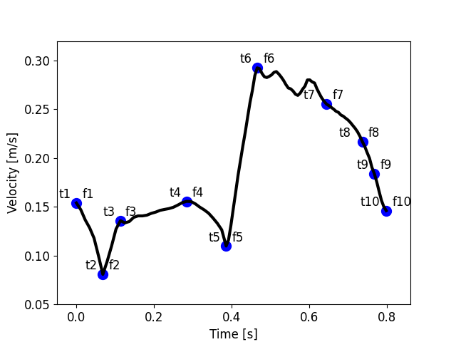
Figure 1: All 20 values labeled on an example waveform. Definitions of points can be found in Table I. Note that each point has a time and velocity component.

II-C Novel stretching transformation

To change the shape of a waveform we propose a novel transformation that can be conceptualized as “stretching”. If one simply changes the value of a point of interest that point will then appear to be discontinuous to the rest of the waveform. We assume that if one point, either time or velocity, increases/decreases then the surrounding points should also increase/decrease.

To stretch the waveform we derive a transformation inspired by linear splines. We take a “base” waveform ($t_{f}$ & $f$) and seek to stretch that waveform so it fits a “target” waveform ($t_{w}$ & $w$). Let $P_{i}$ denote the point of interest $i$ on the base waveform that is being matched, $\hat{P}_{i}$ be the point of interest $i$ on the target waveform, and $p_{k}$ denote the $k^{\text{th}}$ value of the base waveform vectors between the two points of interest $i-1$ and $i$.

Note that $P_{1}$ is matched via addition (translational shift in time and velocity) so this recursive process has an adequate base case. Let $T:\mathbb{R}^{n}\rightarrow\mathbb{R}^{n}$ be the transformation from the base time or velocity vector to the new waveform and $T_{k}:\mathbb{R}\rightarrow\mathbb{R}$ be the operation for entry $k$ out of $n$ total entries. The transformation process for both time and velocity is identical. Thus, we define $T$ as a function of velocity vectors, but it equally applies to time vectors. We define

$$T_{k}(p_{k}) =\underbrace{\frac{p_{k}-P_{i-1}}{P_{i}-P_{i-1}}}_{a_{k}}\underbrace{\left(\hat{P}_{i}-\hat{P}_{i-1}\right)}_{x_{k}}+\underbrace{\hat{P}_{i-1}}_{u_{k}},$$

$$\rightarrow T(f) =a\odot x+u,\hskip 28.45274pta,x,u\in\mathbb{R}^{n},$$

where $\odot$ denotes the Hadamard product (element-wise multiplication). Note that $a$ need only be computed once per base waveform, while $x$ and $u$ need to be computed for each target waveform. An illustration of this stretching operation is depicted in Fig. 2.

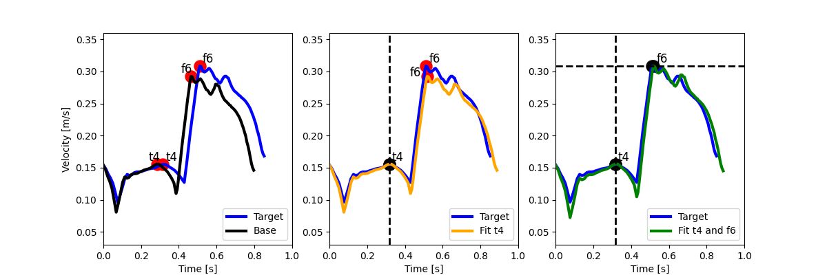
Figure 2: The process of “stretching” waveforms. From left to right, the first panel shows the “base” waveform (black) that will be stretched to match the target (blue) waveform. The second panel shows the result of stretching the waveform along the time axis to match the 4${}^{\text{th}}$ time point (yellow). The third panel shows the result of stretching the waveform in the second panel to match the 6${}^{\text{th}}$ velocity point (green).

II-D Reducing the number of points of interest

Examining all 20 identified points of interest would be a complex task. Furthermore, it would be unclear which points are more important than others. It is also likely that some points are redundant and do not hold insight when other points are used. To find the fewest points needed to characterize a waveform, we seek to find the smallest subset of points that allow an adequate recreation of the target waveforms using the stretching transformation. To assess which subset is best, we begin with a base waveform and fit that waveform to the 1,000 representative waveforms using each possible subset of points while matching the initial time and velocity. Since modulating a waveform has a relatively low computational cost, we can explore each subset of points using a high-performance computing cluster. We calculate our residual through the relative difference in the systolic and diastolic area under the curve [2], as well as the relative two-norm difference ($r_{2}$),

$$r_{2}=\sqrt{\left(\frac{||t_{w}-t_{g}||_{2}}{||t_{w}||_{2}}\right)^{2}+\left(\frac{||w-g||_{2}}{||w||_{2}}\right)^{2}}.$$

III Results

Our results demonstrate the effectiveness of the stretching operation by computing the residual for all possible point combinations. We then identify the optimal sets of points for different set sizes, providing insights into the most efficient ways to quantify the velocity waveform.

III-A Selecting the points of interest from the fitting procedure

To find the best set of points to characterize the waveform of the left coronary artery, we apply our stretching technique to fit a base waveform to the 1,000 representative waveforms chosen. We fitted using every possible set of points and computed the average residual across the 1,000 waveforms. Fig. 3 shows the minimal residual for each set size. For example, of all sets with two points, the set with the smallest residual had a residual of just over 0.1. We observe that set sizes 6 through 12 obtained the same minimal residual. Furthermore, the points of interest that produce the smallest residual for the set size six can be seen in Fig. 4.

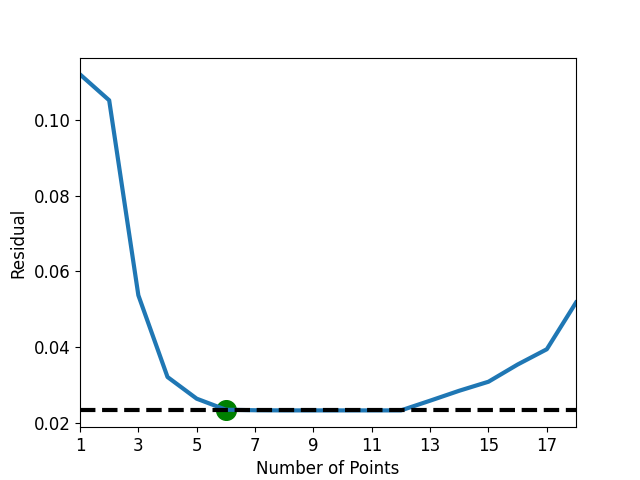
Figure 3: The smallest average residual for each point set size. The dashed horizontal line shows the minimal residual and the green dot denotes the smallest set size that can obtain the minimal residual.

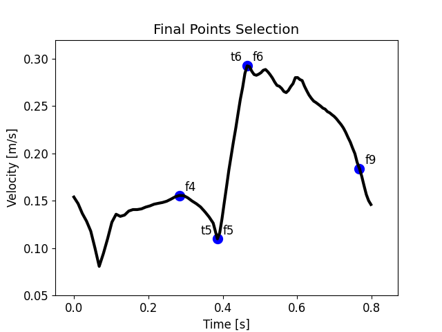
Figure 4: Points of interest that obtain the lowest residual for set size 6 (f4, t5, f5, t6, f6, f9), which corresponds to the green dot in Fig. 3.

IV Discussion

We have developed a pipeline that finds the minimum number of points of interest to quantify a velocity waveform and specifically consider left coronary artery velocity waveforms as proof of concept. We first verified that the proposed points of interest are positively correlated within the time and velocity domains. Once this correlation has been verified, we applied the fitting procedure to the waveforms in question and examined residuals to determine the most efficient way to quantify the velocity waveform.

IV-A Positive Correlations of Time and Velocity Points

The stretching transformation assumes the positive correlation of points. This assumption is most obvious in the time domain. For example, since $t_{i}<t_{i+1}$, if $t_{i}$ increases then $t_{i+1}$ is likely to increase as well. The velocity domain is less obvious, but one can infer that if a velocity point increases, then the rest of the velocity points are also likely to increase as a result of the inertia of blood. Thus, for blood flow velocity waveforms, the stretching procedure is well-founded.

IV-B Selecting the Optimal Points to Characterize a Blood Velocity Waveform

We base our selection of points of interest on the assumption that the points that can best be used to stretch a base waveform to the ones of interest are the most important to the shape of waveforms. This assumption is motivated by the ability of these points to change the shape of the base waveform.

For left coronary arteries we see from Fig. 3 that the minimum residual is present for point set sizes of 6 to 12. In this case, the first set size that achieves the minimum residual is a set with 6 points, however; the difference in residual between a set of 5 points and 6 is minimal, so a set of either 5 or 6 points is both appropriate.

IV-C Applications in the Clinic

Finding the minimum number of points that adequately characterize a waveform is of clinical significance as it will allow clinicians to effectively quantitatively assess waveforms. Previous studies [2, 4] have demonstrated the importance of the area under the systolic and diastolic curves, as well as the maximum velocity, but are coarse metrics. The method presented here allows clinicians to focus on a small number of observable points to characterize the waveform.

IV-D Limitations

In this proof-of-concept study, we used a database of simulated coronary artery waveforms [10]. Future work should apply this pipeline to patient waveforms. We do not label the bump in diastole with a point, as it is difficult to find automatically and preliminary analysis showed that it is minimally relevant to the residual.

IV-E Conclusion

In our study, we introduced a method that efficiently identifies and utilizes the minimal number of significant features from given waveforms. This approach ensures the accurate representation of a waveform’s shape with a reduced set of points. As a practical demonstration, we applied this method to simulated left coronary artery waveforms and discovered that a surprisingly small selection of points suffices to capture waveform variations. This finding opens the door to future research where this pipeline could be applied to a variety of other physiological waveforms for similar efficiency and effectiveness.

References

- [1] Justin E Davies et al. “Use of simultaneous pressure and velocity measurements to estimate arterial wave speed at a single site in humans” In American Journal of Physiology-Heart and Circulatory Physiology 290.2 American Physiological Society, 2006, pp. H878–H885
- [2] Takeshi Hozumi et al. “Noninvasive assessment of coronary flow velocity and coronary flow velocity reserve in the left anterior descending coronary artery by Doppler echocardiography: comparison with invasive technique” In Journal of the American College of Cardiology 32.5 American College of Cardiology Foundation Washington, DC, 1998, pp. 1251–1259
- [3] Fumihiko Kajiya et al. “Velocity profiles and phasic flow patterns in the non-stenotic human left anterior descending coronary artery during cardiac surgery” In Cardiovascular research 27.5 Oxford University Press, 1993, pp. 845–850
- [4] Elizabeth O Ofili, Arthur J Labovitz and Morton J Kern “Coronary flow velocity dynamics in normal and diseased arteries” In The American journal of cardiology 71.14 Elsevier, 1993, pp. D3–D9
- [5] M Schiemann et al. “MR-based coronary artery blood velocity measurements in patients without coronary artery disease” In European radiology 16 Springer, 2006, pp. 1124–1130
- [6] Simbarashe G Chidyagwai et al. “Characterization of hemodynamics in anomalous aortic origin of coronary arteries using patient-specific modeling” In Journal of Biomechanics 132 Elsevier, 2022, pp. 110919
- [7] Noelia Grande Gutierrez et al. “Hemodynamic variables in aneurysms are associated with thrombotic risk in children with Kawasaki disease” In International journal of cardiology 281 Elsevier, 2019, pp. 15–21
- [8] Maurizio Lodi Rizzini et al. “Does the inflow velocity profile influence physiologically relevant flow patterns in computational hemodynamic models of left anterior descending coronary artery?” In Medical Engineering & Physics 82 Elsevier, 2020, pp. 58–69
- [9] Katharine H Fraser et al. “Characterization of an abdominal aortic velocity waveform in patients with abdominal aortic aneurysm” In Ultrasound in medicine & biology 34.1 Elsevier, 2008, pp. 73–80
- [10] Cyrus Tanade et al. “Cloud Computing to Enable Wearable-Driven Longitudinal Hemodynamic Maps” In Proceedings of the International Conference for High Performance Computing, Networking, Storage and Analysis, 2023, pp. 1–14