Testing the Instanton Approach to the Large Amplification Limit of a Diffraction-Amplification Problem

Abstract

The validity of the instanton analysis approach is tested numerically in the case of the diffraction-amplification problem $\partial_{z}\psi-\frac{i}{2m}\partial^{2}_{x^{2}}\psi=g|S|^{2}\,\psi$ for $\ln U\gg 1$, where $U=|\psi(0,L)|^{2}$. Here, $S(x,z)$ is a complex Gaussian random field, $z$ and $x$ respectively are the axial and transverse coordinates, with $0\leq z\leq L$, and both $m\neq 0$ and $g>0$ are real parameters. To sample the rare and extreme amplification values of interest ($\ln U\gg 1$), we devise a specific biased sampling procedure by which $p(U)$, the probability distribution of $U$, is obtained down to values less than $10^{-2270}$ in the far right tail. We find that the agreement of our numerical results with the instanton analysis predictions in Mounaix (2023 J. Phys. A: Math. Theor. 56 305001) is remarkable. Both the predicted algebraic tail of $p(U)$ and concentration of the realizations of $S$ onto the leading instanton are clearly confirmed, which validates the instanton analysis numerically in the large $\ln U$ limit.

I Introduction

In a recent work Mounaix2023 , the instanton analysis approach Raja1982 ; SS1998 ; FKLM1996 was used to determine the tail of $p(U)$, the probability distribution of $U=|\psi(0,L)|^{2}$, for $\ln U\gg 1$, $\psi(x,z)$ being the solution to the diffraction-amplification problem:

$$\left\{\begin{array}[]{l}\partial_{z}\psi(x,z)-\frac{i}{2m}\partial^{2}_{x^{2}}\psi(x,z)=g|S(x,z)|^{2}\psi(x,z),\\ 0\leq z\leq L,\ x\in\Lambda\subset\mathbb{R},\ {\rm and}\ \psi(x,0)=1.\end{array}\right.$$ (1)

Here, $z$ and $x$ respectively denote the axial and transverse coordinates in a domain of length $L$ and (one-dimensional) cross-section $\Lambda$. For technical convenience, we will take for $\Lambda$ the circle of length $\ell$. The boundary condition at $z=0$ is taken to be a constant for simplicity. Both $m\neq 0$ and $g>0$ are real parameters and $S(x,z)$ is a transversally homogeneous complex Gaussian noise with zero mean and normalization $L^{-1}\int_{0}^{L}\langle|S(x,z)|^{2}\rangle\,dz=1$.

From the instanton analysis of the corresponding Martin-Siggia-Rose action, it was found in Mounaix2023 that $S$ concentrates onto long filamentary instantons, $S_{\rm inst}$, as $\ln U\to+\infty$. These filamentary instantons run along specific non-random paths, denoted by $x_{\rm inst}(\cdot)$, that maximize the largest eigenvalue $\mu_{1}[x(\cdot)]$ of the covariance operator $T_{x(\cdot)}$ defined by

$$(T_{x(\cdot)}f)(z)=\int_{0}^{L}C(x(z)-x(z^{\prime}),z,z^{\prime})\,f(z^{\prime})\,dz^{\prime},\ \ \ f(z)\in L^{2}([0,L]),$$ (2)

where $C(x-x^{\prime},z,z^{\prime})=\langle S(x,z)S(x^{\prime},z^{\prime})^{\ast}\rangle$. In equation (2), $x(\cdot)$ is a continuous path in $\Lambda$ satisfying $x(L)=0$, and for the class of $S$ considered in Mounaix2023 , every maximizing path $x_{\rm inst}(\cdot)$ is also continuous with $x_{\rm inst}(L)=0$ (see Mounaix2023 for details). In the most common case of ‘single-filament instantons’ for which there is only one maximizing path, and assuming a non-degenerate $\mu_{1}[x_{\rm inst}(\cdot)]$, one has $S(x,z)\sim S_{\rm inst}(x,z)$ $(\ln U\to+\infty)$ with

$$S_{\rm inst}(x,z)=\frac{c_{1}}{\mu_{\rm max}}\,\int_{0}^{L}C(x-x_{\rm inst}(z^{\prime}),z,z^{\prime})\,\phi_{1}(z^{\prime})\,dz^{\prime},$$ (3)

where $\mu_{\rm max}$ is short for $\mu_{1}[x_{\rm inst}(\cdot)]$, $\phi_{1}$ is the fundamental eigenfunction of $T_{x_{\rm inst}(\cdot)}$, and $c_{1}$ is a complex Gaussian random variable with $\langle c_{1}\rangle=\langle c_{1}^{2}\rangle=0$ and $\langle|c_{1}|^{2}\rangle=\mu_{\rm max}$. The tail of $p(U)$ for $\ln U\gg 1$ can then be deduced from the statistics of $S_{\rm inst}$ as given in equation (3). The result is a leading algebraic tail $\propto U^{-\zeta}$ with $\zeta=(1+1/2\mu_{\rm max}g)$, modulated by a slow varying amplitude (slower than algebraic) Mounaix2023 .

In the absence of a mathematically rigorous proof, the need for checking the validity of these analytical results numerically cannot be overlooked. To this end, it is essential to have a good sampling of the realizations of $S$ for which $\ln U\gg 1$. Unfortunately, such realizations are extremely rare events, far beyond the reach of any direct sampling with a reasonable sample size. For instance, for the same Gaussian field $S$ and parameters as in section $5$ of Mounaix2023 and in the simple diffraction-free limit, $m^{-1}=0$, in which $U$ can be computed exactly, it can be checked that $p(\ln U\geq 10^{3})=O(10^{-100})$. It is thus clearly unrealistic to expect that the asymptotic analytical results can be tested by direct numerical simulations. To gain access to the asymptotic regime and check the validity of the instanton analysis we need a specific approach. One possible strategy is to bias the underlying distribution of $S$ towards the outcomes of interest. In the case of nonlinear equations with additive noise, this has been successfully achieved by means of the ‘importance sampling algorithm’ HM1956 frequently used in rare event physics (see e.g. HDMRS2018 ; HMS2019 and references therein). For the diffraction-amplification problem (1), it turns out that a different, somewhat simpler, method can be devised, based on the existence of a nonlinear fit to numerical data giving a highly accurate approximation of $U$ as a function of $S$, when $\ln U$ is large. It is then possible to determine the extreme upper tail of $p(U)$ and the corresponding realizations of $S$ from numerical simulations. Development of the biased sampling procedure and its application to check the validity of the instanton analysis in the case of problem (1) is the subject of the present work.

Before entering the details of the calculations, it is useful to summarize our main results.

• Let $T_{C}$ denote the covariance operator defined by

  $$(T_{C}f)(x,z)=\int_{0}^{L}\int_{\Lambda}C(x-x^{\prime},z,z^{\prime})\,f(x^{\prime},z^{\prime})\,dx^{\prime}dz^{\prime},\ \ \ f(x,z)\in L^{2}(\Lambda\times[0,L]),$$ (4)

  and $S_{\rm inst}$ the instanton solution given in equation (3). Write $r_{\stretchrel*{\parallel}{\perp}}$, and $r_{\perp}$ the $L^{2}$-norms of the components of $T_{C}^{-1/2}S$ parallel and perpendicular to $T_{C}^{-1/2}S_{\rm inst}$ (in the $L^{2}$ sense). By analyzing a large number of numerical solutions to equation (1), we identify the existence of an implicit equation relating $U$, $r_{\stretchrel*{\parallel}{\perp}}$, and $r_{\perp}$ when $\ln U$ is large and all the other quantities characterizing $T_{C}^{-1/2}S$ are fixed. The reason why $T_{C}^{-1/2}S$ appears rather than $S$ will be made clear at the end of section II and above equation (16). More specifically, writing $r_{\stretchrel*{\parallel}{\perp}}=\sqrt{\eta}\cos\theta$ and $r_{\perp}=\sqrt{\eta}\sin\theta$, with $0\leq\theta\leq\pi/2$ and $\eta>0$, we check that our numerical data satisfy

  $$\cos\theta-\left(\frac{\log_{10}U}{a\eta-b}\right)^{\alpha}=0,$$ (5)

  with very good accuracy for $1820\leq\log_{10}U\leq 2030$ and $1000\leq\eta\leq 1100$, where $a=1.86428$, $b=25.7163$, and $\alpha\sim 0.5$ is a random exponent depending on the quantities characterizing $T_{C}^{-1/2}S$ other than $\theta$ and $\eta$.

• From this result, we derive the expression of the conditional probability distribution $p(U,\theta|\varSigma_{\rm orv})$ valid for $\log_{10}U\gg 1$, where $\varSigma_{\rm orv}$ stands for all the random variables characterizing $T_{C}^{-1/2}S$ other than $\theta$ and $\eta$ (‘orv’ is short for ‘other random variables’). For a given $U$ with $\log_{10}U\gg 1$, we then obtain (i) $p(U|\varSigma_{\rm orv})$ by integrating $p(U,\theta|\varSigma_{\rm orv})$ numerically over $0\leq\theta\leq\pi/2$, and (ii) $p(\theta|U,\varSigma_{\rm orv})$ as $p(U,\theta|\varSigma_{\rm orv})/p(U|\varSigma_{\rm orv})$.

• We draw the realizations of $S$ given $U$ with $\log_{10}U\gg 1$ according to the procedure defined by: (a) draw $\varSigma_{\rm orv}$; (b) derive $p(\theta|U,\varSigma_{\rm orv})$; (c) draw $\theta$ from $p(\theta|U,\varSigma_{\rm orv})$ instead of from its unconditional probability distribution; and (d) use the resulting $T_{C}^{-1/2}S$ in $S=T_{C}^{1/2}(T_{C}^{-1/2}S)$ to get $S$.

• We estimate $p(U)$ as the sample mean of $p(U|\varSigma_{\rm orv})$ over realizations of $\varSigma_{\rm orv}$ for different values of $U$ with $\log_{10}U\gg 1$ and we compare the results with the predictions of the instanton analysis. Let $\mathfrak{D}$ denote the $L^{2}$-distance between $S/\|S\|_{2}$ and $S_{\rm inst}/\|S_{\rm inst}\|_{2}$. For a given $U$ with $\log_{10}U\gg 1$, we estimate $p(\mathfrak{D}|U)$ as a sample mean over realizations of $\varSigma_{\rm orv}$ and $\theta$ (see equation (23) and below). Finally, we plot $|S|^{2}/\|S\|^{2}_{2}$ for different realizations of $S$ with particular values of $\mathfrak{D}$ as well as the sample mean of $|S|^{2}/\|S\|^{2}_{2}$ over realizations of $S$ with close values of $\mathfrak{D}$, and we compare the results with the theoretical instanton profile.

The outline of the paper is as follows. The Gaussian field $S$ that we consider is specified in section II, where we also recall some results of Mounaix2023 needed in the sequel. Section III gives preliminary numerical results used in section IV. Finally, in section IV we define our biased sampling procedure and use it to test the instanton analysis of problem (1) numerically, in the limit of a large $\ln U$.

II Model and definitions

Since the present work is the continuation of the numerical study initiated in Mounaix2023 , section 5, we consider the same Gaussian field $S(x,z)$. Namely, we take

$$S(x,z)=\sum_{\mathclap{n=-50}}^{50}{\vphantom{\sum}}^{\prime}s_{n}\sqrt{\varsigma_{n}}\,\exp\,i\left[\frac{2\pi n}{\ell}x+\left(\frac{2\pi n}{\ell}\right)^{2}\frac{z}{2}\right],$$ (6)

where $\sum_{n}^{\,\prime}$ means $\sum_{n\neq 0}$. Here, the $s_{n}$s are independent and identically distributed (i.i.d.) complex Gaussian random variables with $\langle s_{n}\rangle=\langle s_{n}s_{m}\rangle=0$ and $\langle s_{n}s_{m}^{\ast}\rangle=\delta_{nm}$. The spectral density $\varsigma_{n}$ normalized to $\sum_{n=-50}^{\,\prime\,50}\varsigma_{n}=1$ is given by the Gaussian spectrum

$$\varsigma_{n}\propto\exp\left[-\left(\frac{\pi n}{\ell}\right)^{2}\right].$$ (7)

Equation (6) is reminiscent of models of spatially smoothed laser beams RD1993 , where $S$ is a solution to the paraxial wave equation

$$\partial_{z}S(x,z)+\frac{i}{2}\partial^{2}_{x^{2}}S(x,z)=0,$$ (8)

with boundary condition $S(x,0)=\sum_{n=-50}^{\,\prime\,50}s_{n}\sqrt{\varsigma_{n}}\,\exp(2i\pi nx/\ell)$. The $n=0$ mode is excluded from the Fourier representation (6) to ensure that the space average $\ell^{-1}\int_{\Lambda}S(x,z)\,dx$ is zero for all $z$ and every realization of $S$, as expected for the electric field of a smoothed laser beam.

For each realization of $S$ on a cylinder of length $L=10$ and circumference $\ell=20$, we solve equation (1) by using a symmetrized $z$-split method Strang1968 which propagates the diffraction term, $(i/2m)\partial^{2}_{x^{2}}\psi(x,z)$, in Fourier space and the amplification term, $g|S(x,z)|^{2}\psi(x,z)$, in real space. We take $m=0.7$, and $g=0.5$. For $S$ in equation (6) with Gaussian spectrum (7) and the given values of $L$ and $\ell$, it is shown in Mounaix2023 that:

(i) there is a single instanton, $S_{\rm inst}$, which is a single-filament instanton of the form (3) in which $x_{\rm inst}(\cdot)\equiv 0$, $\mu_{\rm max}=4.34984$, and

$$C(x,z,z^{\prime})=C(x,z-z^{\prime})=\sum_{\mathclap{n=-50}}^{50}{\vphantom{\sum}}^{\prime}\varsigma_{n}\,\exp\,i\left[\frac{2\pi n}{\ell}x+\left(\frac{2\pi n}{\ell}\right)^{2}\frac{z-z^{\prime}}{2}\right];$$ (9)

(ii) the convolution representation of $S_{\rm inst}$ in equation (3) with $x_{\rm inst}(\cdot)\equiv 0$ and $C$ in equation (9) is equivalent to the Fourier representation

$$S_{\rm inst}(x,z)=\sum_{\mathclap{n=-50}}^{50}{\vphantom{\sum}}^{\prime}\mathfrak{s}_{n}\sqrt{\varsigma_{n}}\,\exp\,i\left[\frac{2\pi n}{\ell}x+\left(\frac{2\pi n}{\ell}\right)^{2}\frac{z}{2}\right],$$ (10)

where $\bm{\mathfrak{s}}$ (with components $\mathfrak{s}_{n}$) is an eigenvector of the $100\times 100$ positive definite Hermitian matrix

$$M_{nm}=\sqrt{\varsigma_{n}\varsigma_{m}}\,\int_{0}^{L}\exp i\left[\left(\frac{2\pi}{\ell}\right)^{2}(m^{2}-n^{2})\,\frac{z}{2}\right]\,dz,\ \ \ \ (n,m\neq 0),$$ (11)

associated with the eigenvalue $\mu_{\rm max}$. (Note that $M$ and $T_{x_{\rm inst}(\cdot)\equiv 0}$ have the same eigenvalues with the same degeneracies MCL2006 ). The $\mathfrak{s}_{n}$s in equation (10) are correlated complex Gaussian random variables with $\langle\mathfrak{s}_{n}\rangle=\langle\mathfrak{s}_{n}\mathfrak{s}_{m}\rangle=0$ and $\langle\mathfrak{s}_{n}\mathfrak{s}_{m}^{\ast}\rangle=\mathfrak{e}_{n}^{(1)}\mathfrak{e}^{(1)\,\ast}_{m}$, where $\bm{\mathfrak{e}}^{(1)}$ (with components $\mathfrak{e}_{n}^{(1)}$) is the normalized fundamental eigenvector of $M$ (see Mounaix2023 , section 4.1, for details).

Figure 1 shows the contour plots of $|S_{\rm inst}|^{2}$ and the autocorrelation profile $|C|^{2}$ (also referred to as ‘hot spot profile’ in the laser-matter interaction literature RD1993 ).

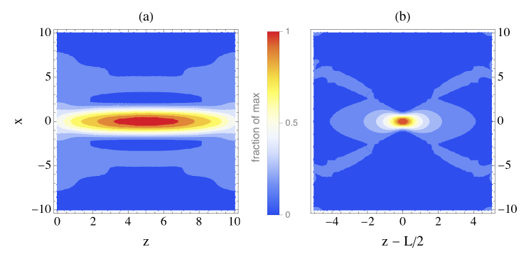
Figure 1: (a) Contour plot of $|S_{\rm inst}(x,z)|^{2}$ for $S_{\rm inst}(x,z)$ in equation (10). (b) Contour plot of the autocorrelation profile (or ‘hot spot profile’) $|C(x,z-L/2)|^{2}$ for $C(x,z-z^{\prime})$ in equation (9). (Color scale legend : $1$ corresponds to the maximum of the plotted function.)

Define $\hat{S}_{\rm inst}=S_{\rm inst}/\|S_{\rm inst}\|_{2}$ and $\hat{S}=S/\|S\|_{2}$ where $\|\cdot\|_{2}$ denotes the $L^{2}$-norm on $\Lambda\times[0,L]$. Write $S_{\parallel}=\left(\hat{S}_{\rm inst},\hat{S}\right)\hat{S}_{\rm inst}$ the component of $\hat{S}$ along $S_{\rm inst}$. We measure the departure of the realizations of $S$ from the instanton through the $L^{2}$-distance

$$\mathfrak{D}=\|\hat{S}-S_{\parallel}\|_{2}=\sqrt{1-|(\hat{S},\hat{S}_{\rm inst})|^{2}}.$$ (12)

Using the Fourier representations (6) and (10) in which we write $\bm{s}$ (with components $s_{n}$) as $\bm{s}=\|\bm{s}\|\,\hat{\bm{s}}$ and $\bm{\mathfrak{s}}=\|\bm{\mathfrak{s}}\|\,\hat{\bm{\mathfrak{s}}}$ with $\hat{\bm{\mathfrak{s}}}={\rm e}^{i\,{\rm arg}(c_{1})}\bm{\mathfrak{e}}^{(1)}$, where $\|\cdot\|$ is the usual Euclidean norm and where we have used $\bm{\mathfrak{s}}=\mu_{\rm max}^{-1/2}c_{1}\bm{\mathfrak{e}}^{(1)}$ (see the first equation (52) in Mounaix2023 ), one gets

$$\mathfrak{D}=\sqrt{1-\frac{|\sum_{n}^{\,\prime}\varsigma_{n}\hat{s}_{n}\mathfrak{e}_{n}^{(1)\,\ast}|^{2}}{\left(\sum_{n}^{\,\prime}\varsigma_{n}|\hat{s}_{n}|^{2}\right)\,\left(\sum_{n}^{\,\prime}\varsigma_{n}|\mathfrak{e}_{n}^{(1)}|^{2}\right)}},$$ (13)

which is the counterpart of the equation (66) in Mounaix2023 for fixed $y=0\,$.

From equations (4), (6), and (9) it can be checked that the $s_{n}$s are also the components of $T_{C}^{-1/2}S$ in the orthonormal function basis $(1/\sqrt{\ell L})\,\exp i[2\pi nx/\ell+(2\pi n/\ell)^{2}z/2]$, which trivially defines an isomorphism between the $T_{C}^{-1/2}S$-space with $L^{2}$-inner product and the $\bm{s}$-space with usual dot product. As we will see shortly, for $S$ given by equation (6) our results come out naturally in terms of $\bm{s}$, and therefore $T_{C}^{-1/2}S$, which explains why it is $T_{C}^{-1/2}S$ that appears in the summary at the end of section I, rather than $S$.

We now have everything we need to move on to the presentation of our biased sampling method and its application to check the validity of the results obtained in Mounaix2023 . This is the subject of the next two sections.

III Preliminary results

According to instanton analysis, the larger $\log_{10}U$ the more $\bm{s}$ tends to align with $\bm{\mathfrak{e}}^{(1)}$. Testing the instanton analysis in the large $\log_{10}U$ regime therefore requires a good sampling of $\bm{s}$ around the direction of $\bm{\mathfrak{e}}^{(1)}$. To do this, we need to control the direction of $\bm{s}$, which can be achieved by a change of variables making the direction and amplitude of $\bm{s}$ explicit.

Write $N$ the number of terms in the sum on the right-hand side of equation (6) ($N=100$). A given realization of $S$ corresponds to a given realization of the (complex) $N$-dimensional vector $\bm{s}$ with coordinates $s_{n}$, and conversely. Let $\hat{\bm{u}}$ be a given $N$-dimensional (complex) unit vector, not necessarily equal to $\bm{\mathfrak{e}}^{(1)}$. Define $\bm{s}_{\stretchrel*{\parallel}{\perp}}=(\bm{s}\cdot\hat{\bm{u}}^{\ast})\,\hat{\bm{u}}=r_{\stretchrel*{\parallel}{\perp}}{\rm e}^{i\varphi}\hat{\bm{u}}$ and $\bm{s}_{\perp}=\bm{s}-\bm{s}_{\stretchrel*{\parallel}{\perp}}=r_{\perp}\,\hat{\bm{s}}_{\perp}$ with $r_{\perp}=\|\bm{s}_{\perp}\|$. Switching to polar coordinates $r_{\stretchrel*{\parallel}{\perp}}=\sqrt{\eta}\cos\theta$ and $r_{\perp}=\sqrt{\eta}\sin\theta$, with $\eta=\|\bm{s}\|^{2}$ and $0\leq\theta\leq\pi/2$, we characterize the realizations of $S$ by the new variables $\theta$, $\eta$, $\varphi$, and $\hat{\bm{s}}_{\perp}$. The polar angle $\theta$ measures how close the direction of $\bm{s}$ is to that of $\hat{\bm{u}}$: $\theta=0$ means that $\bm{s}$ is aligned with $\hat{\bm{u}}$ ($\bm{s}_{\perp}=0$), whereas $\theta=\pi/2$ means that $\bm{s}$ is orthogonal to $\hat{\bm{u}}$ ($\bm{s}_{\stretchrel*{\parallel}{\perp}}=0$).

The statistical properties of the new variables are deduced from the ones of the $s_{n}$s. Since the $s_{n}$s are i.i.d. standard complex Gaussian random variables, the projection of $\bm{s}$ onto any given direction is also a standard complex Gaussian random variable independent of the projections onto the orthogonal directions. This applies in particular to $s_{\stretchrel*{\parallel}{\perp}}=(\bm{s}\cdot\hat{\bm{u}}^{\ast})$ and the components of $\bm{s}_{\perp}$. After some straightforward algebra, one finds that the probability distribution functions (pdf) of $\theta$ and $\eta$ are respectively given by

$$f(\theta)=2(N-1)\,(\sin\theta)^{2N-3}\cos\theta\,\bm{1}_{0\leq\theta\leq\pi/2},$$ (14)

and

$$h(\eta)=\Gamma(N)^{-1}\,\eta^{N-1}{\rm e}^{-\eta}\,\bm{1}_{0\leq\eta}.$$ (15)

The random phase $\varphi$ and tip of $\hat{\bm{s}}_{\perp}$ (i.e. the direction of $\bm{s}_{\perp}$) are uniformly distributed over $[0,2\pi)$ and the sphere $\|\bm{s}_{\perp}\|=1$, respectively.

It now remains to set the reference direction $\hat{\bm{u}}$. Until the instanton analysis has been validated, we cannot rule out the possibility that realizations of $\bm{s}$ with $\hat{\bm{s}}$ away from $\bm{\mathfrak{e}}^{(1)}$ may contribute significantly to a large $\log_{10}U$. Taking $\hat{\bm{u}}=\bm{\mathfrak{e}}^{(1)}$, as suggested by the instanton analysis, must first be justified numerically. To ensure that $\hat{\bm{u}}=\bm{\mathfrak{e}}^{(1)}$ is indeed safe, we compared results for $\hat{\bm{u}}=\bm{\mathfrak{e}}^{(1)}$ and orthogonal directions $\hat{\bm{u}}=\bm{\mathfrak{e}}^{(q\geq 2)}$, where $\bm{\mathfrak{e}}^{(q)}$ is the normalized eigenvector of $M$ associated with the $q$th largest eigenvalue $\mu_{q}$ ($1\leq q\leq N$). (For the Gaussian spectrum (7), we have checked numerically that none of the $\mu_{q}$s is degenerate.)

In figures 2 and 3, we show results for $\hat{\bm{u}}=\bm{\mathfrak{e}}^{(1)}$ and $\hat{\bm{u}}=\bm{\mathfrak{e}}^{(2)}$ (with $\mu_{1}=\mu_{\rm max}=4.34984$ and $\mu_{2}=2.0126$). Figure 2 shows scatter plots of $\theta$ and numerically computed $\log_{10}U$ for a given realization of $\varphi$ and $\hat{\bm{s}}_{\perp}$, fixed $\eta=1060$, and $10^{3}$ ascending values of $\theta$ regularly spaced by $\Delta\theta=0.263\ 10^{-3}$ starting from $\theta=0$. Figures 2(a) and (b) correspond to $\hat{\bm{u}}=\bm{\mathfrak{e}}^{(1)}$ and $\hat{\bm{u}}=\bm{\mathfrak{e}}^{(2)}$, respectively. Figure 3 shows the results for $\hat{\bm{u}}=\bm{\mathfrak{e}}^{(1)}$ with $\eta=1060$ and $\hat{\bm{u}}=\bm{\mathfrak{e}}^{(2)}$ with larger $\eta=1880$, each for two different realizations of $\varphi$ and $\hat{\bm{s}}_{\perp}$. For better legibility, only $50$ of the $10^{3}$ points actually computed are shown in figure 3.

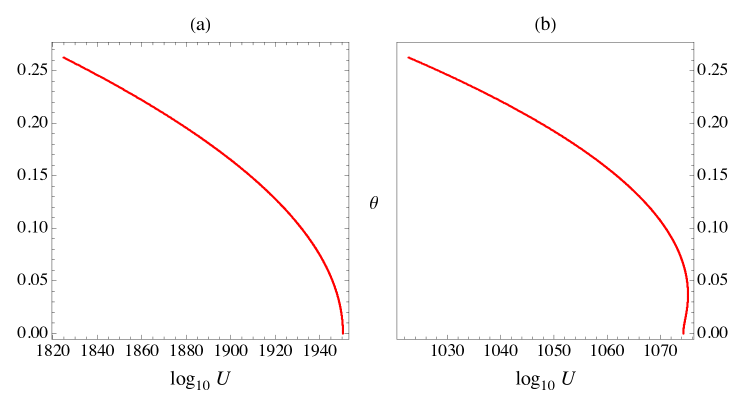
Figure 2: Scatter plots of $\theta$ and $\log_{10}U$ for a given realization of $\varphi$ and $\hat{\bm{s}}_{\perp}$, fixed $\eta=1060$, and two different (orthogonal) reference directions: (a) $\hat{\bm{u}}=\bm{\mathfrak{e}}^{(1)}$ and (b) $\hat{\bm{u}}=\bm{\mathfrak{e}}^{(2)}$.

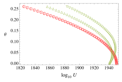
Figure 3: Scatter plots of $\theta$ and $\log_{10}U$ for two different realizations of $\varphi$ and $\hat{\bm{s}}_{\perp}$, each represented by a specific marker. Large and small red circles are for $\hat{\bm{u}}=\bm{\mathfrak{e}}^{(1)}$ with $\eta=1060$, up and down green triangles correspond to $\hat{\bm{u}}=\bm{\mathfrak{e}}^{(2)}$ with $\eta=1880$. (For better legibility, only $50$ of the $10^{3}$ points actually computed are shown.)

For a given $\eta\gg 1$, figure 2 shows that $\log_{10}U$ is significantly smaller in the case $\hat{\bm{u}}=\bm{\mathfrak{e}}^{(2)}$ (figure 2(b)) than for $\hat{\bm{u}}=\bm{\mathfrak{e}}^{(1)}$ (figure 2(a)). To have comparable values of $\log_{10}U$ we need a larger $\eta$ for $\hat{\bm{u}}=\bm{\mathfrak{e}}^{(2)}$ than for $\hat{\bm{u}}=\bm{\mathfrak{e}}^{(1)}$. To be more precise, for $\hat{\bm{u}}=\bm{\mathfrak{e}}^{(2)}$ we have checked that data with $\log_{10}U\gtrsim 1820$ — the smallest value in figure 2(a) — require $\eta\gtrsim 1760$. For instance, it can be seen in figure 3 that it takes $\eta\simeq 1880$ to bring the data for $\hat{\bm{u}}=\bm{\mathfrak{e}}^{(2)}$ in the same range of $\log_{10}U$ as for $\hat{\bm{u}}=\bm{\mathfrak{e}}^{(1)}$ in figure 2(a). Given the fast decreasing tail of $h(\eta)$ in equation (15), an important consequence of this result is that among data falling in the same $(\log_{10}U,\theta)$ region as in figure 3, the proportion of realizations of $\hat{\bm{s}}$ biased towards $\bm{\mathfrak{e}}^{(2)}$ is completely negligible compared to that of realizations biased towards $\bm{\mathfrak{e}}^{(1)}$, typically by a factor less than $h(1760)/h(1060)=O(10^{-282})$. We have checked that the proportion of realizations of $\hat{\bm{s}}$ biased towards $\bm{\mathfrak{e}}^{(q\geq 3)}$ is by far even smaller.

For a given realization of $\varphi$ and $\hat{\bm{s}}_{\perp}$, both figures 2 and 3 show that the data collapse on a single well-defined curve in the $(\log_{10}U,\theta)$ plane. For $\hat{\bm{u}}=\bm{\mathfrak{e}}^{(2)}$, a change in the realization of $\hat{\bm{s}}_{\perp}$ visibly affects the curve (see up and down green triangles in figure 3), which means that the contribution of $\bm{s}_{\perp}$ to the amplification is not negligible in this case. In contrast, for $\hat{\bm{u}}=\bm{\mathfrak{e}}^{(1)}$ we observe that the curve depends very little on the direction of $\bm{s}_{\perp}$ (small and large red circles in figure 3). We have checked that the sensitivity to $\hat{\bm{s}}_{\perp}$ observed for $\hat{\bm{u}}=\bm{\mathfrak{e}}^{(2)}$ is even more pronounced for $\hat{\bm{u}}=\bm{\mathfrak{e}}^{(q\geq 3)}$. Furthermore, as $q$ increases, a dispersion of the data around the curve in the $(\log_{10}U,\theta)$ plane becomes visible and increases with $q$.

The numerical results in figures 2 and 3 show that when $\log_{10}U$ is large, amplification is most likely and mainly determined by realizations of $\bm{s}$ with $\|\bm{s}\|\gg 1$ and direction biased towards $\bm{\mathfrak{e}}^{(1)}$. For fixed $\eta$ and $\theta$, the value of $\log_{10}U$ depends only weakly on the (subdominant) contributions of the components of $\bm{s}$ orthogonal to $\bm{\mathfrak{e}}^{(1)}$. This corroborates the conclusions of instanton analysis and justifies taking $\hat{\bm{u}}=\bm{\mathfrak{e}}^{(1)}$, which will be the case from now on, without fear of missing significant realizations.

Notational remark: it may be useful to briefly come back to the notations used in sections I and III. As explained at the end of section II, $\bm{s}$ and $\bm{\mathfrak{s}}$ are respectively isomorphic to $T_{C}^{-1/2}S$ and $T_{C}^{-1/2}S_{\rm inst}$. Consequently, $r_{\stretchrel*{\parallel}{\perp}}$ and $r_{\perp}$ are also the $L^{2}$-norms of the components of $T_{C}^{-1/2}S$ parallel and perpendicular to $T_{C}^{-1/2}S_{\rm inst}$ (in the $L^{2}$ sense), as written in section I. The quantities characterizing $T_{C}^{-1/2}S$ other than $\theta$ and $\eta$, denoted by $\varSigma_{\rm orv}$ in section I, are the random variable $\varphi$ and vector $\hat{\bm{s}}_{\perp}$.

In figure 4 we show scatter plots of $\theta$ and $\log_{10}U$ for a given realization of $\varphi$ and $\hat{\bm{s}}_{\perp}$, and four different values of $\eta$ (see caption for details). Solid lines correspond to the nonlinear fit

$$\theta=\cos^{-1}\left(\frac{\log_{10}U}{a\eta-b}\right)^{\alpha(\bm{s})},$$ (16)

where $a=1.86428$, $b=25.7163$, and $\alpha(\bm{s})$ is a realization dependent exponent. Data points and nonlinear fits match remarkably well. We have checked on $10^{2}$ realizations of $\varphi$ and $\hat{\bm{s}}_{\perp}$, $10$ values of $\eta$ between $1010$ and $1100$, and $10^{3}$ values of $\theta$ like in figure 2 (which represents a total of $10^{6}$ different realizations of $S$), that for each $\varphi$, $\hat{\bm{s}}_{\perp}$, and $\eta$, the $10^{3}$ data points and the nonlinear fit are practically indistinguishable over the whole range $1820\leq\log_{10}U\leq 2030$. Numerical results also show that (i) no systematic (monotonic) variation of $\alpha(\bm{s})$ with $\eta$ at fixed $\varphi$ and $\hat{\bm{s}}_{\perp}$ is observed in the range of $\eta$ considered, and (ii) the relative dispersion of $\alpha(\bm{s})$ for different values of $\eta$ at fixed $\varphi$ and $\hat{\bm{s}}_{\perp}$ is one order of magnitude less than for different realizations of $\varphi$ and $\hat{\bm{s}}_{\perp}$ at fixed $\eta$ : $\Delta\alpha(\bm{s})/\langle\alpha(\bm{s})\rangle=10^{-3}$ and $10^{-2}$, respectively. Thus, with a good accuracy level, it is not unreasonable to ignore the dependence of $\alpha(\bm{s})$ on $\eta$ and write $\alpha(\bm{s})=\alpha(\varphi,\hat{\bm{s}}_{\perp})$. We have checked by replacing $\alpha(\bm{s})$ in equation (16) with values obtained for different $\eta$ and the same realization of $\varphi$ and $\hat{\bm{s}}_{\perp}$, all other things being equal, that the error made in the nonlinear fit is indeed imperceptible.

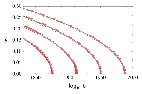
Figure 4: Scatter plots of $\theta$ and $\log_{10}U$ for a given realization of $\varphi$ and $\hat{\bm{s}}_{\perp}$, and four different values of $\eta$ (down red triangles). Solid lines are plots of the nonlinear fit (16) for the corresponding $\eta$ and numerically computed $\alpha(\bm{s})$. Parameter values are $(\eta,\alpha(\bm{s}))=(1020,0.52569)$, $(1040,0.524924)$, $(1060,0.524862)$, and $(1080,0.525024)$, from left to right. (In each plot, only $50$ of the $10^{3}$ points actually computed are shown.)

We now use these results to write $p(U)$ and conditional probability $P(\mathcal{A}|U)$, where $\mathcal{A}$ is a set of realizations of $\bm{s}$, in forms suitable to numerical estimates in the asymptotic regime $\log_{10}U\gg 1$. Write $U(\bm{s})=|\psi_{\bm{s}}(0,L)|^{2}$, $\psi_{\bm{s}}(x,z)$ being the solution to equation (1) for a given $S$ (hence $\bm{s}$). Our numerical results show that inverting equation (16) gives a highly accurate approximation of $U(\bm{s})$ when $\log_{10}U\gg 1$. Replacing $U(\bm{s})$ with this approximation in the exact expression $p(U)=\left\langle\delta(U-U(\bm{s}))\right\rangle_{\bm{s}}$, where $\langle\cdot\rangle_{\bm{s}}$ denotes the average over the realizations of $\bm{s}$, one obtains

$$p(U) = \frac{1}{\ln 10}\,\frac{1}{U}\left\langle\int_{0}^{+\infty}\int_{0}^{\pi/2}\delta\left[\log_{10}U-(\cos\theta)^{1/\alpha(\varphi,\hat{\bm{s}}_{\perp})}(a\eta-b)\right]f(\theta)h(\eta)\,d\theta d\eta\right\rangle_{\varphi,\hat{\bm{s}}_{\perp}}$$ (17)

$$= \frac{1}{\ln 10}\,\frac{1}{U}\left\langle\int_{0}^{\pi/2}\frac{f(\theta)}{a\,(\cos\theta)^{1/\alpha(\varphi,\hat{\bm{s}}_{\perp})}}\,h\left(\frac{\log_{10}U}{a\,(\cos\theta)^{1/\alpha(\varphi,\hat{\bm{s}}_{\perp})}}+\frac{b}{a}\right)\,d\theta\right\rangle_{\varphi,\hat{\bm{s}}_{\perp}}$$

$$= \left\langle\int_{0}^{\pi/2}p(U,\theta|\varphi,\hat{\bm{s}}_{\perp})\,d\theta\right\rangle_{\varphi,\hat{\bm{s}}_{\perp}},$$

with

$$p(U,\theta|\varphi,\hat{\bm{s}}_{\perp})=\frac{1}{\ln 10}\,\frac{f(\theta)}{Ua\,(\cos\theta)^{1/\alpha(\varphi,\hat{\bm{s}}_{\perp})}}\,h\left(\frac{\log_{10}U}{a\,(\cos\theta)^{1/\alpha(\varphi,\hat{\bm{s}}_{\perp})}}+\frac{b}{a}\right).$$ (18)

The expression for $p(\mathcal{A},U)$ is similar to equation (17) with integrand $\bm{1}_{\bm{s}\in\mathcal{A}}\,p(U,\theta|\varphi,\hat{\bm{s}}_{\perp})$, where $\bm{s}=\sqrt{\eta}\cos\theta\,{\rm e}^{i\varphi}\bm{\mathfrak{e}}^{(1)}+\sqrt{\eta}\sin\theta\,\hat{\bm{s}}_{\perp}$ with $\eta=a^{-1}(b+\log_{10}U/(\cos\theta)^{1/\alpha(\varphi,\hat{\bm{s}}_{\perp})})$. Dividing this expression by $p(U)$ one obtains

$$P(\mathcal{A}|U)=\left\langle w_{\alpha(\varphi,\hat{\bm{s}}_{\perp})}(U)\int_{0}^{\pi/2}\bm{1}_{\bm{s}\in\mathcal{A}}\,p(\theta|U,\varphi,\hat{\bm{s}}_{\perp})\,d\theta\right\rangle_{\varphi,\hat{\bm{s}}_{\perp}},$$ (19)

with

$$p(\theta|U,\varphi,\hat{\bm{s}}_{\perp})=\frac{p(U,\theta|\varphi,\hat{\bm{s}}_{\perp})}{p(U|\varphi,\hat{\bm{s}}_{\perp})},$$ (20)

and

$$w_{\alpha(\varphi,\hat{\bm{s}}_{\perp})}(U)=\frac{p(U|\varphi,\hat{\bm{s}}_{\perp})}{p(U)}.$$ (21)

In equations (20) and (21), $p(U|\varphi,\hat{\bm{s}}_{\perp})$ is obtained by integrating equation (18) numerically over $0\leq\theta\leq\pi/2$ (for fixed $U$ and a given realization of $\varphi$ and $\hat{\bm{s}}_{\perp}$). Equations (17) to (21) give the expressions of $p(U)$ and $P(\mathcal{A}|U)$ valid for $\log_{10}U\gg 1$.

IV Biased sampling and numerical validation of instanton analysis

Let $\{\varphi,\hat{\bm{s}}_{\perp}\}$ denote the same sample of $10^{2}$ independent realizations of $\varphi$ and $\hat{\bm{s}}_{\perp}$ as the one we used to check the validity of the nonlinear fit in equation (16). Figure 5 shows plots of $p(\theta|U,\varphi,\hat{\bm{s}}_{\perp})$ for three different realizations in $\{\varphi,\hat{\bm{s}}_{\perp}\}$ and $\log_{10}U=1890$. Curves (a), (b), and (c) correspond to the realizations of $\{\varphi,\hat{\bm{s}}_{\perp}\}$ yielding the smallest, middle, and largest values of $p(U|\varphi,\hat{\bm{s}}_{\perp})$, respectively. Diamonds correspond to $p(\theta|U)$ computed as the sample mean of $p(\theta|U,\varphi,\hat{\bm{s}}_{\perp})$ for the realizations in $\{\varphi,\hat{\bm{s}}_{\perp}\}$.

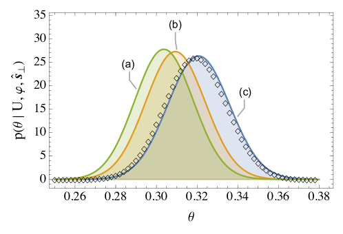
Figure 5: Plots of $p(\theta|U,\varphi,\hat{\bm{s}}_{\perp})$ for fixed $\log_{10}U=1890$ and three particular realizations in $\{\varphi,\hat{\bm{s}}_{\perp}\}$ corresponding to the smallest (a), middle (b), and largest (c) values of $p(U|\varphi,\hat{\bm{s}}_{\perp})$. Plot of $p(\theta|U)$ for the same value of $\log_{10}U=1890$ (diamonds).

For a given $\log_{10}U\gg 1$ and realizations of $\varphi$ and $\hat{\bm{s}}_{\perp}$ in $\{\varphi,\hat{\bm{s}}_{\perp}\}$, the statistically significant realizations of $S$ are those for which $\theta$ is in the bulk of $p(\theta|U,\varphi,\hat{\bm{s}}_{\perp})$. Figure 5 and similar results obtained for different values of $U$ with $1820\leq\log_{10}U\leq 1940$ show that a good sampling of the corresponding significant values of $\theta$, requires probing the whole range $0.25\leq\theta\leq 0.38$. Since the equation (14) yields $P(0.25\leq\theta\leq 0.38)=5.2\ 10^{-86}$, it is clear that having $\theta$ in that range is an extremely rare event, virtually impossible to sample directly by drawing $\theta$ from $f(\theta)$. By contrast, it can easily be achieved by drawing $\theta$ from $p(\theta|U,\varphi,\hat{\bm{s}}_{\perp})$ rather than from $f(\theta)$. This is what defines our biased sampling procedure which consists of the following four steps:

• draw $\varphi$ and $\hat{\bm{s}}_{\perp}$ from the uniform distributions over $[0,2\pi)$ and the sphere $\|\bm{s}_{\perp}\|=1$, respectively;

• compute $\alpha(\varphi,\hat{\bm{s}}_{\perp})$ by making the graph of the function in equation (16) fit the data in the $(\log_{10}U,\theta)$ region of interest, for some fixed $\eta$. (We have checked that for $1820\leq\log_{10}U\leq 2030$, $\eta$ can be chosen arbitrarily between $1010$ and $1100$;)

• use the result in equation (18) to get $p(U,\theta|\varphi,\hat{\bm{s}}_{\perp})$. For fixed $U$ (with $\log_{10}U\gg 1$), integrate the result numerically over $0\leq\theta\leq\pi/2$ to get $p(U|\varphi,\hat{\bm{s}}_{\perp})$. Then, draw $\theta$ from $p(\theta|U,\varphi,\hat{\bm{s}}_{\perp})$ in equation (20) and set $\eta$ by inverting equation (16);

• the outcome defines a realization of $\bm{s}=\sqrt{\eta}\cos\theta\,{\rm e}^{i\varphi}\bm{\mathfrak{e}}^{(1)}+\sqrt{\eta}\sin\theta\,\hat{\bm{s}}_{\perp}$ which, once injected onto the right-hand side of equation (6), gives a realization of $S(x,z)$.

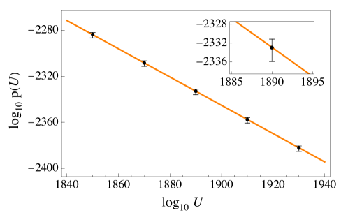
Figure 6: $\log_{10}p(U)$ a a function of $\log_{10}U$ from $1850$ to $1930$ by steps of $20$, with $p(U)$ given by equation (22) (black dots). Smallest and largest $p(U|\varphi,\hat{\bm{s}}_{\perp})$ in the sample are indicated by the ends of vertical bars. Plot of $\log_{10}p(U)=-\zeta\log_{10}U+{\rm Const}$ with $\zeta=(1+1/2\mu_{\rm max}g)=1.22989$ given by instanton analysis and ${\rm Const}=-8.41526$ adjusted to get the best fit to numerical data (solid line). Inset: enlargement of the same plot near $\log_{10}U=1890$.

From the data for $p(U|\varphi,\hat{\bm{s}}_{\perp})$ obtained as explained in step (C) for each realization in $\{\varphi,\hat{\bm{s}}_{\perp}\}$ and fixed $U$, we have estimated $p(U)$ as the sample mean

$$p(U)=\frac{1}{{\rm card}\{\varphi,\hat{\bm{s}}_{\perp}\}}\,\sum_{(\varphi,\hat{\bm{s}}_{\perp})\in\{\varphi,\hat{\bm{s}}_{\perp}\}}p(U|\varphi,\hat{\bm{s}}_{\perp}).$$ (22)

Figure 6 shows the results in the $(\log_{10}U,\log_{10}p(U))$ plane for five different values of $U$ with $\log_{10}U$ between $1840$ and $1940$. Black dots correspond to $p(U)$. The dispersion of $p(U|\varphi,\hat{\bm{s}}_{\perp})$ around $p(U)$ is indicated by vertical bars the ends of which correspond to the smallest and largest values of $p(U|\varphi,\hat{\bm{s}}_{\perp})$ in the sample. The error bars corresponding to the standard deviation of the sample mean (22) are found to be eight times shorter, in the case of figure 6 (not shown). Instanton analysis predicts a leading algebraic tail of $p(U)\propto U^{-\zeta}$ with $\zeta=(1+1/2\mu_{\rm max}g)=1.22989$. The solid line is the plot of $\log_{10}p(U)=-\zeta\log_{10}U+{\rm Const}$, where ${\rm Const}=-8.41526$ has been adjusted to get the best fit to the data. We observe an almost perfect alignment of numerical data along a straight line with slope $-\zeta$, which validates the result of instanton analysis numerically in the considered range of $\log_{10}U$. Note also the extremely small value of $p(U)<10^{-2270}$ which confirms, if need be, the absolute impossibility of sampling the extreme upper tail of $p(U)$ directly, without a specific bias procedure.

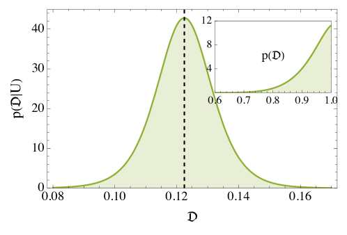
Figure 7: $p(\mathfrak{D}|U)$ for fixed $\log_{10}U=1890$ estimated from a biased sample of $10^{6}$ realizations of $S$ drawn according to the biased sampling procedure defined in steps (A) to (D) (see the text for details). The median of $p(\mathfrak{D}|U)$ is at $\mathfrak{D}=0.122457$ (dashed line). Inset: $p(\mathfrak{D})$ estimated from an unbiased sample of $10^{5}$ realizations of $S$.

The question then arises of the realizations of $S$ behind the results in figure 6. According to the instanton analysis in Mounaix2023 , these realizations should be instanton realizations with the same profile as in figure 1(a). For a given $U$, the way $S$ differs from the instanton can be characterized by the conditional pdf $p(\mathfrak{D}|U)$, where $\mathfrak{D}$ is the $L^{2}$-distance defined in equation (13). For each element of $\{\varphi,\hat{\bm{s}}_{\perp}\}$ and fixed $U$, we drew $10^{4}$ independent realizations of $\theta$ — denoted in the following by $\{\theta|\varphi,\hat{\bm{s}}_{\perp}\}$ — as explained in step (C). For definiteness, we took $\log_{10}U=1890$ at the center of the range considered in figure 6. There are $10^{2}$ subsamples $\{\theta|\varphi,\hat{\bm{s}}_{\perp}\}$ of $10^{4}$ elements each, representing a total of $10^{6}$ different realizations of $\bm{s}$. For each $\bm{s}$, we have used the equation (13) to compute the corresponding value of $\mathfrak{D}$. We have then estimated $P(\mathfrak{D}\leq\delta|U)$ in equation (19) with $\mathcal{A}=\{\bm{s}|\mathfrak{D}\leq\delta\}$ as the sample mean

$$P(\mathfrak{D}\leq\delta|U)=\frac{1}{{\rm card}\{\varphi,\hat{\bm{s}}_{\perp}\}}\,\sum_{(\varphi,\hat{\bm{s}}_{\perp})\in\{\varphi,\hat{\bm{s}}_{\perp}\}}\,\frac{w_{\alpha(\varphi,\hat{\bm{s}}_{\perp})}(U)}{{\rm card}\{\theta|\varphi,\hat{\bm{s}}_{\perp}\}}\,\sum_{\theta\in\{\theta|\varphi,\hat{\bm{s}}_{\perp}\}}\bm{1}_{\mathfrak{D}\leq\delta},$$ (23)

from which $p(\mathfrak{D}|U)$ is obtained by (numerical) derivation with respect to $\delta$ at $\delta=\mathfrak{D}$. Figure 7 shows the result for $\log_{10}U=1890$. For comparison, we show in inset the pdf of $\mathfrak{D}$ obtained from an unbiased sample of $10^{5}$ realizations of $S$. The vertical dashed line indicates the median of $p(\mathfrak{D}|U)$ at $\mathfrak{D}=\tilde{\mathfrak{D}}=0.122457$. (The median, mean and maximum of $p(\mathfrak{D}|U)$ are all at $\tilde{\mathfrak{D}}$, to within numerical accuracy.) It can be seen that the realizations of $S$ conditioned to a large $\log_{10}U\gg 1$ are significantly closer to the instanton than unconditioned realizations: $0.08<\mathfrak{D}<0.16$ and $0.6<\mathfrak{D}\leq 1$, respectively, in the case of figure 7. This is in agreement with the instanton analysis in Mounaix2023 which predicts $\mathfrak{D}\rightarrow 0$ in probability, as $\log_{10}U\rightarrow+\infty$.

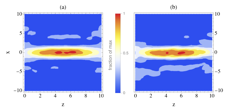
Figure 8: Contour plots of $|\hat{S}(x,z)|^{2}$ for two realizations of $S$ with $\mathfrak{D}\simeq 0.08$ (a) and $\mathfrak{D}\simeq 0.16$ (b).

In figure 8, we show $|\hat{S}(x,z)|^{2}=|S(x,z)|^{2}/\|S\|_{2}^{2}$ for two realizations of $S$ with $\mathfrak{D}\simeq 0.08$ and $\mathfrak{D}\simeq 0.16$, on both sides of the bulk of $p(\mathfrak{D}|U)$. Figure 9(a) shows the same quantity for a realization with $\mathfrak{D}\simeq\tilde{\mathfrak{D}}$, right at the center of the bulk of $p(\mathfrak{D}|U)$. The results in figures 8(a), 8(b), and 9(a) are very similar and typical of the realizations generated by the biased sampling procedure for $\log_{10}U=1890$. These realizations are the superposition of an elongated cigar-shaped component along $x=0$ and fluctuations of comparatively small amplitude. Fluctuations can be smoothed out by averaging realizations of $|\hat{S}|^{2}$ close together along the $\mathfrak{D}$ axis, bringing out the underlying cigar-shaped component. To this end, we have constructed five subsamples $\{S\}_{\mathfrak{D}=\delta}$ of $10^{2}$ realizations of $S$ selected by picking in the total (biased) sample the $50$ realizations with largest values of $\mathfrak{D}\leq\delta$ and the $50$ realizations with smallest values of $\mathfrak{D}>\delta$, for $\delta=0.1$, $0.11$, $\tilde{\mathfrak{D}}\,(=0.122457)$, $0.13$, and $0.14$. Then, we have computed the sample means of $|\hat{S}(x,z)|^{2}$ for the realizations in each $\{S\}_{\mathfrak{D}=\delta}$. In figure 9(b), we show the result for $\delta=\tilde{\mathfrak{D}}$. (The smallest and largest values of $\mathfrak{D}$ for $S$ in $\{S\}_{\mathfrak{D}=\tilde{\mathfrak{D}}}$ are $0.122403$ and $0.122504$, respectively.) We have obtained identical results for the five different values of $\delta$ we have considered.

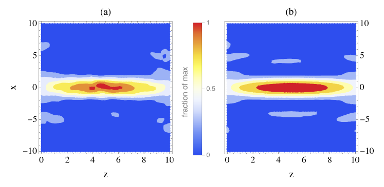
Figure 9: (a) Contour plot of $|\hat{S}(x,z)|^{2}$ for a realization of $S$ with $\mathfrak{D}\simeq\tilde{\mathfrak{D}}$. (b) Contour plot of the sample mean of $|\hat{S}(x,z)|^{2}$ for the $10^{2}$ realizations in $\{S\}_{\mathfrak{D}=\tilde{\mathfrak{D}}}$ (with $0.122403\leq\mathfrak{D}\leq 0.122504$).

The close resemblance between figures 9(b) and 1(a) is obvious and the dominant cigar-shaped component of $|\hat{S}|^{2}$ along $x=0$ visible in figures 8(a), 8(b), and 9(a) can clearly be identified as the theoretical instanton profile. These results, together with the small values of $\mathfrak{D}$ observed in figure 7, show that the realizations of $S$ conditioned on a large but finite $\log_{10}U$ (here, $\log_{10}U=1890$) are low-noise instanton realizations. This is in agreement with the instanton analysis in Mounaix2023 which predicts noiseless instanton realizations in the limit $\log_{10}U\rightarrow+\infty$.

The numerical results in figures 6 to 9 show remarkable agreement with the analytical predictions of instanton analysis. Data points for $\log_{10}p(U)$ and $\log_{10}U$ line up almost perfectly along the predicted algebraic tail $\log_{10}p(U)\simeq-\zeta\log_{10}U$ with $\zeta=(1+1/2\mu_{\rm max}g)$ (figure 6), and the corresponding realizations of $S$ are observed to be heavily biased towards the predicted instanton realizations (figures 7 to 9). In conclusion, we can say that our results provide a convincing numerical validation of the instanton analysis in the large amplification regime $\log_{10}U\gg 1$.

V Summary

In this paper, we have numerically tested the validity of the instanton analysis approach to study the diffraction-amplification problem (1) in the large amplification regime $\ln U\gg 1$, where $U=|\psi(0,L)|^{2}$, $\psi(x,z)$ being the solution to equation (1). By analyzing a large number of numerical solutions to equation (1), we have identified a nonlinear fit to numerical data from which a highly accurate approximation of $U$ as a function of $S$ can be obtained, when $\ln U$ is large (equation (16)). We have then used this result to devise a sampling procedure of $S$ giving access to large values of $\ln U$.

As a first application, we have obtained $p(U)$ numerically over a large range of $U$ with $\ln U\gg 1$, down to probability density less than $10^{-2270}$ in the tail. We have found a near-perfect agreement with the algebraic tail of $p(U)$ theoretically predicted by the instanton analysis in Mounaix2023 (figure 6). Then, we have determined the conditional probability distribution of $\mathfrak{D}$ given $U$ for a large $\ln U$, where $\mathfrak{D}$ is the $L^{2}$-distance measuring the departure of $S$ from the theoretical instanton normalized such that $0\leq\mathfrak{D}\leq 1$. We have found that the realizations of $S$ in the far right tail of $p(U)$ are significantly closer to the instanton than unconditioned realizations: $0.08<\mathfrak{D}<0.16$ and $0.6<\mathfrak{D}\leq 1$ respectively, in the case of figure 7. As a confirmation of this result, plots of $|S|^{2}/\|S\|^{2}_{2}$ clearly show that the realizations of $S$ in the far right tail of $p(U)$ are low-noise instanton realizations around the predicted, noiseless, theoretical instanton, with residual noise due to $\ln U$ being finite (figures 8 and 9). To summarize, our numerical results validate the instanton analysis of the diffraction-amplification problem (1), in the large $\ln U$ limit.

References

(1) Mounaix Ph 2023 J. Phys. A: Math. Theor.56 305001
(2) Rajaraman R 1982 Solitons and Instantons: an Introduction to Solitons and Instantons in Quantum Field Theory (Amsterdam: North-Holland)
(3) Schäfer T and Shuryak E V 1998 Rev. Mod. Phys.70 323
(4) Falkovich G, Kolokolov I, Lebedev V and Migdal A 1996 Phys. Rev. E54 4896
(5) Rose H A and DuBois D F 1994 Phys. Rev. Lett.72 2883
(6) Hammersley J M and Morton K W 1956 Math. Proc. Cambridge Philos. Soc.52 449
(7) Hartmann A K, Le Doussal P, Majumdar S N, Rosso A and Schehr G 2018 Europhys. Lett.121 67004
(8) Hartmann A K, Meerson B and Sasorov P 2019 Phys. Rev. Research1 032043
(9) Rose H A and DuBois D F 1993 Phys. Fluids B5 590
(10) Strang G 1968 SIAM J. Numer. Anal.5 (3) 506
(11) Mounaix Ph, Collet P and Lebowitz J L 2006 Commun. Math. Phys.264 741 and 2008 Commun. Math. Phys.280 281