Semi-parametric financial risk forecasting incorporating multiple realized measures

Abstract

A semi-parametric joint Value-at-Risk (VaR) and Expected Shortfall (ES) forecasting framework employing multiple realized measures is developed. The proposed framework extends the quantile regression using multiple realized measures as exogenous variables to model the VaR. Then, the information from realized measures is used to model the time-varying relationship between VaR and ES. Finally, a measurement equation that models the contemporaneous dependence between the quantile and realized measures is used to “complete” the model. A quasi-likelihood, built on the asymmetric Laplace distribution, enables the Bayesian inference for the proposed model. An adaptive Markov Chain Monte Carlo method is used for the model estimation. The empirical section evaluates the performance of the proposed framework with six stock markets from January 2000 to June 2022, covering the period of COVID-19. Three realized measures, including 5-minute realized variance, bi-power variation, and realized kernel, are incorporated and evaluated in the proposed framework. One-step-ahead VaR and ES forecasting results of the proposed model are compared to a range of parametric and semi-parametric models, lending support to the effectiveness of the proposed framework.

Keywords: Semi-parametric; realized measures; Markov chain Monte Carlo; Value-at-Risk; Expected Shortfall.

1 Introduction

Financial risk management is an integral task for financial institutions. VaR is a standard tool for measuring and controlling financial market risks. Let $\mathcal{L}$ denote the information available at time $t$ and

$F_{t}(r)=Pr(r_{t}\leq r\mid\mathcal{L}_{t-1})$

be the Cumulative Distribution Function (CDF) of the return $r_{t}$ conditional on $\mathcal{L}_{t-1}$. Assuming that $F_{t}(\cdot)$ is strictly increasing and continuous on the real line $\mathbb{R}$, the one-step-ahead $\alpha$-level Value-at-Risk (VaR) at time $t$ can be defined as:

$Q_{t}=F_{t}^{-1}(\alpha),\quad 0<\alpha<1.$

However, VaR cannot measure the magnitude of the loss for violations and is not mathematically coherent, meaning that it is not a sub-additive measure and can favour non-diversification. Artzner . (1999) propose an alternative called Expected Shortfall (ES), also called conditional VaR or tail VaR. ES calculates the expected loss conditional on exceeding a VaR threshold and is a coherent risk measure. The one-step-ahead $\alpha$-level ES is the tail conditional expectation of $r_{t}$, i.e.:

$\textup{ES}_{t}=E(r_{t}\mid r_{t}\leq Q_{t,}\mathcal{L}_{t-1}).$

The recent Basel III Accord places new emphasis on ES, as illustrated in its document MAR Calculation of RWA for credit risk that says: “Reflects revisions in the standardised and internal models approach for market risk, including the shift to an expected shortfall measure.” (Basel Committee on Banking Supervision (2023), p. 2). Our paper focuses on the daily forecasting of VaR and ES on the lower/left tail. According to the Basel III Accord, the common $\alpha=2.5\%$ probability level is employed.

Volatility plays a crucial role in parametric tail risk forecasting. The GARCH model (Engle (1982); Bollerslev (1986)) is widely used for modelling and forecasting volatility in the finance industry. Numerous extensions, such as EGARCH by Nelson (1991) and GJR-GARCH by Glosten . (1993), have been introduced to capture the well-known leverage effect. However, the volatility dynamics in these conventional GARCH models are driven by (daily) returns, which are considered as potentially noisy signals for the volatility series.

The availability of high-frequency intra-day data has allowed construction of many informative, efficient realized measures (RMs) of volatility. The most commonly used RMs include Realized variance (RV) (Andersen  Bollerslev (1998), Andersen . (2003)), Realized Range (RR) (Christensen  Podolskij (2007), Martens  Van Dijk (2007)), Realized Kernel (RK) (Barndorff-Nielsen . (2009), and Bi-power variation (BV) (Barndorff-Nielsen  Shephard (2004)), etc.

Hansen . (2012) include a realized measure in their volatility equation via their realized GARCH framework, also enabling joint modelling of returns and realized measures using a measurement equation. Hansen  Huang (2016) extended the realized GARCH framework to include multiple realized measures, via the Realized Exponential GARCH (REGARCH) model. The REGARCH shows improved volatility forecasting performance compared to realized GARCH, and GARCH, demonstrating the usefulness of incorporating multiple realized measures in volatility modelling.

The tail risk forecasting accuracy of parametric models depends heavily on the choice of error distribution. Semi-parametric models, which are free from such choice, are also developed in the literature. Engle  Manganelli (2004) introduce the conditional auto-regressive VaR (CAViaR) model, which directly estimates VaR as the quantile of the conditional return distribution, optimized by minimising the quantile loss function, for which VaR is strictly consistent. However, CAViaR models do not estimate ES, while further ES is not even elicitable, see Fissler  Ziegel (2016).

Fissler  Ziegel (2016) show that VaR and ES are jointly elicitable for a class of joint loss functions. This has significant implications in the risk forecasting literature, as it opens up new paths, especially for researchers in the field of semi-parametric risk forecasting, to explore joint VaR and ES modelling. Taylor (2019) proposes a framework, called ES-CAViaR, to jointly and semi-parametrically estimate VaR and ES. A quasi-likelihood, built on the asymmetric Laplace (AL) distribution, allows the joint estimation of conditional VaR and ES. Taylor (2019) shows that the quasi-likelihood function falls into the class of strictly consistent loss functions developed by Fissler  Ziegel (2016). In the ES-CAViaR model, a CaViaR-type quantile equation models the VaR component. Then, ES is modelled via two proposed versions of a VaR to ES relationship: additive and multiplicative.

Gerlach  Wang (2020) incorporate a realized measure as an exogenous variable, extending ES-CAViaR models to the semi-parametric ES-X-CAViaR-X model class, finding improved VaR and ES forecast performance. Wang . (2023) further extend the work of Gerlach  Wang (2020) by introducing the semi-parametric Realized-ES-CAViaR framework, including a measurement equation to model the relationship between the tail risk measure and RM; the leverage effect is also included.

Three key facts motivate the development of the proposed framework. First, the REGARCH, using multiple RMs to model volatility, demonstrates improved performance compared to realized GARCH, using only one RM. Second, the REGARCH is a parametric model, requiring the specification of a return error distribution, while semi-parametric models, such as ES-CAViaR, do not; which has been found to be advantageous in many real return series. Third, incorporating a single RM into the semi-parametric modelling process, such as the ES-X-CAViaR-X or Realized-ES-CAViaR, can further improve risk forecasting accuracy. Therefore, in the literature, there is a gap regarding semi-parametric joint VaR and ES forecasting models with multiple realized measures; filling that gap is the primary aim of this paper.

The main contributions of this paper follow. First, a new semi-parametric joint VaR and ES forecasting framework incorporating multiple RMs is proposed. This extends the quantile regression framework using multiple RMs as exogenous variables. The relationship between VaR and ES is modelled as time-varying and driven by the information from RMs. Further, a measurement equation is included in the framework to model the joint contemporaneous dependencies between the quantile series and multiple RMs. Second, an adaptive Bayesian MCMC algorithm is used to estimate the proposed model, including the parameters in the measurement equation variance-covariance matrix. Lastly, the effectiveness of the proposed framework is evaluated via a comprehensive empirical study, including 29 competing models and covering the period from January 2000 to June 2022.

This paper is organized as follows. Section 2 reviews the relevant existing literature on tail risk forecasting models. Section 3 presents the proposed framework. The likelihood function and the adaptive Bayesian MCMC algorithm are presented in section 4. Section 5 presents the empirical results. Section 6 concludes the paper.

2 Background models

This section describes the relevant models used to forecast VaR and ES in the literature, while the properties of each model are described in the context of motivating the proposed framework. Fundamental concepts used in the model development process are also discussed.

2.1 Parametric GARCH-type models

Let $\mathbf{r}=\left\{r_{t},t=1,\ldots,T\right\}$ be a time series of daily returns. The key interest in parametric volatility modelling is the conditional variance, $\sigma_{t}^{2}=\operatorname{var}\left(r_{t}\mid\mathcal{L}_{t-1}\right),$ where $\mathcal{L}_{t-1}$ denotes the $\sigma$-field of information up to and including time $t-1$. $\sigma_{t}$ is called the volatility. Here, $\mathop{\mathbb{E}}(r_{t}|\mathcal{L}_{t-1})=0$ is assumed, equivalent to working with demeaned returns in practice. The GARCH(1,1) model is:

$r_{t}=\sigma_{t}z_{t},$

$\sigma^{2}_{t}=\omega_{0}+\alpha_{1}r^{2}_{t-1}+\beta_{1}\sigma^{2}_{t-1},$

where $z_{t}\overset{\mathrm{i.i.d}}{\sim}\mathcal{D}(0,1)$; $D$ is a 0 mean, unit variance white noise process. Parametric approaches to GARCH requires the parametric return distribution $D$ to be chosen, e.g., Normal, to produce the VaR (quantile) and ES forecasts.

Francq  Zakoïan (2015) and Gao  Song (2008) consider a semi-parametric, approach using historical simulation (HS), by modelling VaR and ES as constant multiples of the latent volatility $\sigma_{t}$, assumed to follow a GARCH-type volatility model. Assuming a constant conditional return distribution with zero mean, the VaR and ES are modelled as:

$$Q_{t} =a_{\alpha}\sigma_{t};\text{ES}_{t}=b_{\alpha}\sigma_{t},$$ (1)

$$\frac{\text{ES}_{t}}{Q_{t}} =\frac{b_{\alpha}}{a_{\alpha}}=c_{\alpha},$$

where $a_{\alpha},b_{\alpha}$ and $c_{\alpha}\geq 1$ are constant and depend on the return distribution and can be estimated via HS on the standardized residuals $\frac{r_{t}}{\hat{\sigma}_{t}}$. The series $\hat{\sigma}_{t}$ is estimated first using quasi-maximum likelihood (QML) (Gao  Song, 2008).

2.2 Realized (E)GARCH model

A parametric realized GARCH framework, incorporating the realized measure into the volatility modelling process via a measurement equation, is developed in Hansen . (2012). Hansen  Huang (2016) further extend the realized GARCH by incorporating multiple realized measures, and propose the parametric realized EGARCH (REGARCH) model. A log-REGARCH specification can be defined as:

$$r_{t} =\sigma_{t}z_{t},$$ (2)

$$\mathrm{log}(\sigma_{t}) =\omega+\beta\mathrm{log}(\sigma_{t-1})+\tau_{1}z_{t-1}+\tau_{2}\left(z_{t-1}^{2}-1\right)+\boldsymbol{\gamma}^{T}\mathbf{u}_{t-1},$$

$$\mathrm{log}(x_{j,t}) =\xi_{j}+\varphi_{j}\mathrm{log}(\sigma_{t})+\delta_{j,1}z_{t}+\delta_{j,2}(z_{t}^{2}-1)+{u}_{j,t},;j=1,2,...,K.$$

The three log-REGARCH equations, in order, are the return equation, the GARCH or volatility equation, and the measurement equation, respectively. The measurement equation defines the contemporaneous relationship between the (ex-post) realized measures of volatility and the (ex-ante) volatility. Here $K$ denotes the number of realized measures and $K=1$ defines the original realized GARCH model. $\mathbf{x}_{t}=(x_{1,t},...,x_{K,t})^{T}$ is the vector of RMs, at time $t$, on the same scale as $\sigma_{t}$, e.g., $\sqrt{RV}$. $z_{t}\stackrel{{\scriptstyle\text{i.i.d.}}}{{\sim}}D_{1}\left(0,1\right)$ and $\mathbf{u}_{t}\stackrel{{\scriptstyle\text{i.i.d.}}}{{\sim}}N\left(0,\Sigma\right)$, where $\mathbf{u}_{t}=(u_{1,t},u_{2,t},...,u_{K,t})^{T}$, and $z_{t}$ and $\mathbf{u}_{t}$ are mutually and serially independent. Further, the coefficient $\boldsymbol{\gamma}=(\gamma_{1},...,\gamma_{K})^{T}$ of $\mathbf{u}_{t-1}$ represents how informative the realized measures of day $t-1$ are about volatility on day $t$. The model uses two sets of leverage functions, both following the usual quadratic form, to model the leverage effect.

2.3 Semi-parametric ES-X-CAViaR-X model

Taylor (2019) proposes a semi-parametric class of models (called ES-CAViaR) to model the dynamics of VaR and ES jointly. Gerlach  Wang (2020) extend this model by adding various different ES to VaR relationships, allowing a single RM to influence both VaR and ES separately. One of their proposed semi-parametric ES-X-CAViaR-X models is defined as follows:

$$Q_{t} =\beta_{0}+\beta_{1}x_{t-1}+\beta_{2}Q_{t-1},$$ (3)

$$\omega_{t} =\gamma_{0}+\gamma_{1}x_{t-1}+\gamma_{2}\omega_{t-1},$$

$$\text{ES}_{t} =Q_{t}-\omega_{t}.$$

Here $x_{t}$ is the RM. The dynamics of $\text{ES}_{t}$ and $Q_{t}$ have an additive, time-varying relationship, defined by $\omega_{t}$, which is driven, separately to $Q_{t}$, by the RM. The specification of $\omega_{t}$ is directly generalized from a GARCH-type model. This specification allows the unknown conditional return distribution to change over time. The restriction $\gamma_{0}\geq 0,\gamma_{1}\geq 0,\gamma_{2}\geq 0$ is employed to ensure that the VaR and ES series do not cross.

2.4 Semi-parametric Realized-ES-CAViaR models

The semi-parametric Realized-ES-CAViaR models (Wang ., 2023) extend the ES-X-CAViaR-X model by incorporating a measurement equation:

$$Q_{t} =\beta_{0}+\beta_{1}x_{t-1}+\beta_{2}Q_{t-1},$$ (4)

$$\omega_{t} =\gamma_{0}+\gamma_{1}x_{t-1}+\gamma_{2}\omega_{t-1},$$

$$\text{ES}_{t} =Q_{t}-\omega_{t},$$

$$x_{t} =\xi+\phi|\text{Q}_{t}|+\tau_{1}\epsilon_{t}+\tau_{2}\left(\epsilon^{2}_{t}-E(\epsilon^{2})\right)+u_{t},$$

where $\gamma_{0}\geq 0,\gamma_{1}\geq 0,\gamma_{2}\geq 0$ is used again to ensure VaR and ES do not cross. The multiplicative error $\epsilon_{t}=\frac{r_{t}}{Q_{t}}$ in the measurement equation facilitates the modelling of the leverage effect. Again VaR and ES are influenced by the RM separately, via the difference $\omega_{t}$. Again the unknown conditional return distribution changes over time as the relationship between VaR and ES is time-varying and driven by the RM. Compared to the ES-X-CAViaR-X model (Gerlach  Wang, 2020), the added measurement equation “completes” the model by regressing the RM on the quantile (can also be replaced with ES).

3 Proposed Model

This paper proposes a new Realized-ES-CAViaR-M model, employing multiple RMs to jointly and semi-parametrically model VaR and ES. The model extends the Realized-ES-CAViaR, via incorporating multiple RMs and adding a log specification, as well as the REGARCH, by virtue of being semi-parametric, i.e. the return distribution assumption is not required. The proposed model is specified as:

$$\mathrm{log}(|Q_{t}|) =\beta_{0}+\beta_{1}\mathrm{log}{(|Q_{t-1}|)}+\tau_{1}\epsilon_{t-1}+\tau_{2}(\epsilon_{t-1}^{2}-E(\epsilon^{2}))+\boldsymbol{\gamma}^{T}\mathbf{u}_{t-1},$$ (5)

$$\omega_{t} =\nu_{0}+\nu_{1}\omega_{t-1}+\boldsymbol{\psi}^{T}\mathbf{|{u}|}_{t-1},$$ (6)

$$\text{ES}_{t} =Q_{t}-\omega_{t},$$ (7)

$$\mathrm{log}(x_{j,t}) =\xi_{j}+\phi_{j}\mathrm{log}(|Q_{t}|)+\delta_{j,1}\epsilon_{t}+\delta_{j,2}(\epsilon_{t}^{2}-E(\epsilon^{2}))+\mathbf{u}_{j,t};j=1,2,...,K.$$ (8)

The model contains four equations: the quantile equation (5), the VaR-ES difference $\omega_{t}$ equation (6), the ES equation (7) and the measurement equations (8). As in REGARCH, $K$ is the number of realized measures and $K=1$ gives a log spefication of the Realized-ES-CAViaR. Here $x_{t}$ is the square root of the RM, i.e. on the same scale as volatility. The measurement error vector $\mathbf{u}_{t}\stackrel{{\scriptstyle\text{i.i.d.}}}{{\sim}}N\left(0,\Sigma\right)$, as standard. $\Sigma$ is the variance-covariance matrix of $\mathbf{u}_{t}$, with dimension $K\times K$. The multiplicative error $\epsilon_{t}=\frac{r_{t}}{Q_{t}}$ is defined as for the Realized-ES-CAViaR. The key developments of the model are now discussed.

The (1st) quantile equation extends the existing quantile regression (CAViaR, Engle  Manganelli (2004)) by introducing a log specification, including the leverage effect term and incorporating the information from multiple RMs. This makes the model ananlogous to REGARCH. This paper studies the left tail quantile, e.g., $\alpha=2.5\%$; thus, each quantile $Q_{t}<0$; thus $|Q_{t}|$ is used in the log operator. The leverage effect is captured as in the Realized-ES-CAViaR. The regression coefficients $\boldsymbol{\gamma}^{T}$ capture how influential the $K$ lagged RMs are on next period (log-)quantiles.

The 2nd ($\omega_{t}$) and 3rd (ES) equations, (6) and (7), capture the time varying and additive relationship between VaR and ES, all driven separately by the lagged RM vector, whose individual effects on the VaR to ES difference are given by $\boldsymbol{\psi}^{T}$, where $\boldsymbol{\psi}=(\psi_{1},...,\psi_{K})^{T}$. Again we constrain $\nu_{0}\geq 0,\nu_{1}\geq 0,\boldsymbol{\psi}\geq 0$ to ensure that the VaR and ES series do not cross. Other relationships between VaR and ES, such as the multiplicative one in Taylor (2019), could also be explored (though that one implies a constant conditional return distribution).

The measurement equation (8) completes the model by providing a way to model the joint contemporaneous dependence between the risk level and multiple RMs $x_{j,t};j=1,2,...,K$. The leverage function is included in the usual manner.

4 Likelihood and model estimation

CAViaR-type models are typically estimated via minimising the quantile loss function, for which the latent quantile series is strictly consistent. Engle  Manganelli (2004) employ a multiple start approach, to find optimal initial values for the estimation procedure, an approach also employed by Taylor (2019) estimating ES-CAViaR type models; there the loss function is a joint loss for VaR and ES, based on the Asymmetric Laplace (AL) distribution. Via comprehensive simulation study, Gerlach  Wang (2020) and Wang . (2023) find that the Bayesian estimator can be more accurate than direct minimisation of the joint loss as in Taylor (2019). Thus, this paper also employs Bayesian methods.

4.1 Likelihood function for the proposed model

As discussed in Sections 2.3 and 2.4, the ES-CAViaR, ES-X-CAViaR-X and Realized-ES-CAViaR models are semi-parametric in nature. However, Bayesian methods typically employ a parametric distributional assumption to form a likelihood.

Koenker  Machado (1999) note that the conventional quantile regression estimator is equivalent to an MLE based on the AL density, with a mode at the quantile. Discovering a specific link between $\text{ES}_{t}$ and a dynamic $\sigma_{t}$, for the AL distribution, Taylor (2019) further extends this result to produce the conditional density function:

$$f_{t}(r)=\frac{(\alpha-1)}{\text{ES}_{t}}\exp\left(\frac{(r_{t}-Q_{t})(\alpha-I(r_{t}\leq Q_{t}))}{\alpha\text{ES}_{t}}\right),$$ (9)

As shown in Taylor (2019), the negative logarithm of this AL-based density function is strictly consistent for $Q_{t}$ and $\text{ES}_{t}$ jointly, meaning that it fits into the class of strictly consistent loss functions developed by Fissler  Ziegel (2016).

This density then allows a likelihood function to be built, given models for $Q_{t}$ and $\text{ES}_{t}$, and assuming a zero mean return, thus allowing Bayesian methods to be employed. Since $r_{t}$ cannot actually follow an AL distribution with a mode at $Q_{t}$, the AL-based likelihood built on Equation (9) is a quasi-likelihood function, whose mode coincides with the minimum of the joint loss function. The quasi log-likelihood is then:

$$\ell(\mathbf{r};\mbox{\boldmath$\theta$})=\sum_{t=1}^{T}\left(\log\frac{(\alpha-1)}{\text{ES}_{t}}+\frac{(r_{t}-Q_{t})(\alpha-I(r_{t}\leq Q_{t}))}{\alpha\text{ES}_{t}}\right),$$ (10)

where $\mathbf{r}=\left\{r_{1},r_{2},...r_{T}\right\}$ and the parameter vector is $\theta$.

The full model likelihood also includes parts from the measurement equations. The AL-based return log-likelihood (10) combines with the likelihood for the RMs to produce the full quasi log-likelihood for the proposed Realized-ES-CAViaR-M model:

$$\ell(\mathbf{r},\mathbf{X};\mbox{\boldmath$\theta$},\Sigma)=\ell(\mathbf{r};\mbox{\boldmath$\theta$})+\ell(\mathbf{X}|\mathbf{r};\mbox{\boldmath$\theta$},\Sigma),$$

where $\mathbf{X}$ is the set of multiple RMs: $\{x_{1,t},x_{2,t},\ldots,x_{K,t}\}$ and $\Sigma$ is the covariance matrix of the measurement errors $\mathbf{u}_{t}$. Thus, the full quasi log-likelihood of the proposed model can be written as:

$$\begin{split}\ell(\mathbf{r},\mathbf{X};\mbox{\boldmath$\theta$},\Sigma)=&\sum_{t=1}^{n}\left(\log\frac{(\alpha-1)}{\text{ES}_{t}}+\frac{(r_{t}-Q_{t})(\alpha-I(r_{t}\leq Q_{t}))}{\alpha\text{ES}_{t}}\right)\\ &-\frac{1}{2}\sum_{t=1}^{n}\left(k\log(2\pi)+\log(\left|\Sigma\right|)+\mathbf{u}_{t}^{{}^{\prime}}\Sigma^{-1}\mathbf{u}_{t}\right),\end{split}$$ (11)

For any given value of $\theta$, Hansen  Huang (2016) show that the RM based Gaussian likelihood yields the partial maximization concerning $\Sigma$ as:

$$\hat{\Sigma}(\theta)=\frac{1}{n}\sum_{t=1}^{n}\mathbf{u}_{t}(\theta){\mathbf{u}_{t}(\theta)^{{}^{\prime}}},$$

where they point out that $\mathbf{u}_{t}$ in the above equation depends on $\theta$, but does not depend on the covariance matrix $\Sigma$. So the maximization problem is simplified to finding arg $\textup{max}_{\theta}\ell(\mathbf{r},\mathbf{X};\mbox{\boldmath$\theta$},\hat{\Sigma{(\theta}}))$ since

$$\sum_{t-1}^{n}\mathbf{u}_{t}^{{}^{\prime}}(\theta)\Sigma(\theta)^{-1}\mathbf{u}_{t}(\theta)=tr\left\{\sum_{t=1}^{n}\hat{\Sigma}(\theta)^{-1}\mathbf{u}_{t}(\theta)\mathbf{u}_{t}^{{}^{\prime}}(\theta)\right\}=nK$$

which does not depend on $\theta$.

From a Bayesian standpoint, the likelihood has the form of an inverse Wishart distribution in $\Sigma$, which could then be integrated out from the likelihood, if desired. However, we decided to keep it in to allow Bayesian inference on $\Sigma$.

4.2 Bayesian estimation

Priors are chosen to be uninformative over the regions sufficient for non-negativity of $\omega_{t}$ in equation (6), combined with other, quite liberal and wide, limits to ensure finite parameter ranges and a proper prior. Thus, $\pi(\mbox{\boldmath$\theta$})\propto I(A)$, being a flat prior for $\theta$ over the region $A$, and 0 elsewhere. To ensure finite parameter ranges, $A$ restricts $-D_{0}<\mbox{\boldmath$\theta$}<D_{0}$. For $\beta_{1}$, stationarity requires $|\beta_{1}|<1$, i.e. $D_{0}=1$. In the empirical study, for the other parameters, we choose $D_{0}=3$, which is sufficiently large based on our analyses. To ensure non-negativity of $\omega_{t}$, region $A$ further restricts $\nu_{0}\geq 0,\nu_{1}\geq 0,\boldsymbol{\psi}\geq 0$. A standard Jeffreys prior $\frac{1}{\Sigma_{jj}}$ is employed for the scale parameters $\Sigma_{jj}$ in the variance and covariance matrix $\Sigma$, whose determinant is restricted to be non-negative, as required in (11).

Following Chen . (2022), in the MCMC algorithm, to assist with speed of mixing, the parameter vector is simulated in blocks from the conditional posterior. Blocks are chosen so that parameters not in the same block are less correlated, in the posterior, whilst parameters within each block tend to be more correlated in the posterior; this aids faster mixing and convergence. Table 1 details the blocking structure, based on the number of RMs in the model. The block-wise proposals are generated and accepted with the usual Metropolis acceptance probability, e.g. see Chen . (2022). $B_{i}$ represents the parameters block $i^{th}$. In the empirical study, we consider $K=1;2;3$.

Table 1: Block structure of the employed MCMC

Block number	k=1 (13 parameters)	k=2 (21 parameters)	k=3 (30 parameters)
$B_{1}$	$\left\{\beta_{0},\beta_{1},\tau_{1},\tau_{2}\right\}$	$\left\{\beta_{0},\beta_{1},\tau_{1},\tau_{2}\right\}$	$\left\{\beta_{0},\beta_{1},\tau_{1},\tau_{2}\right\}$
$B_{2}$	$\left\{\gamma,\Sigma_{11}\right\}$	$\left\{\gamma_{1},\gamma_{2}\right\}$	$\left\{\gamma_{1},\gamma_{2},\gamma_{3}\right\}$
$B_{3}$	$\left\{\delta 11,\delta_{12}\right\}$	$\left\{\xi_{1},\xi_{2}\right\}$	$\left\{\xi_{1},\xi_{2},\xi_{3}\right\}$
$B_{4}$	$\left\{\nu_{0},\nu_{1}\right\}$	$\left\{\phi_{1},\phi_{2}\right\}$	$\left\{\phi_{1},\phi_{2},\phi_{3}\right\}$
$B_{5}$	$\left\{\xi,\phi,\psi\right\}$	$\left\{\delta_{11},\delta_{12},\delta_{21},\delta_{22}\right\}$	$\left\{\delta_{11},\delta_{21},\delta_{31}\right\}$
$B_{6}$		$\left\{\nu_{0},\nu_{1}\right\}$	$\left\{\delta_{12},\delta_{22},\delta_{32}\right\}$
$B_{7}$		$\left\{\psi_{1},\psi_{2}\right\}$	$\left\{\nu_{0},\nu_{1}\right\}$
$B_{8}$		$\left\{\Sigma_{11},\Sigma_{22},\Sigma_{12}\right\}$	$\left\{\psi_{1},\psi_{2},\psi_{3}\right\}$
$B_{9}$			$\left\{\Sigma_{11},\Sigma_{22},\Sigma_{33}\right\}$
$B_{10}$			$\left\{\Sigma_{12},\Sigma_{13},\Sigma_{23}\right\}$

The proposal density is a mixture of three multivariate Gaussian proposal distributions, with a random walk mean vector for each block. The proposal variance-covariance matrix of each block in each mixture element is $C_{i}\Sigma$, where $C_{1}=1;C_{2}=100;C_{3}=0.01$, with $\Sigma$ initially set to $\frac{2.38}{\sqrt{(d_{i})}}I_{d_{i}}$, where $d_{i}$ is the dimension of the $i^{th}$ block and $I_{d_{i}}$ is the identity matrix of dimension $d_{i}$. The vector of mixing weights $(w)$ is (0.7, 0.15, 0.15) allowing both small and large proposal jumps to be considered. The covariance matrix for each block is tuned as in Chen . (2022), with target acceptance rates as in Roberts . (1997); i.e. acceptance rates: 0.44% for $d_{i}=1$, 0.35 when $2\leq d_{i}\leq 4$ and 0.234 for $d_{i}>4$. The algorithm is run for $N=150,000$ iterations to ensure the MCMC convergence. The last 5,000 iterates are used for estimation and inference.

5 Data and Empirical study

5.1 Data description

Daily closing prices and RM data from January 2000 to June 2022 are downloaded from Oxford-man Institute’s realized library (Heber ., 2009). Three common RMs, including Realized variance (5 minutes) (RV5), Realized kernel (RK), and Bi-power variation (BV) are considered. Six market indices, including S&P500 and NASDAQ in the US, FTSE 100 (UK), DAX (Germany), SMI (Swiss), and HSI (Hong Kong), are included in the study. Each data set is split into an initial in-sample period, from January 2000 to December 2011, and an out-of-sample forecasting period from January 2012 to June 2022. Our in-sample period includes the global financial crisis (GFC) and the COVID-19 period. Figure 1 displays a time series plot of the absolute value of daily return, RV5, RK and BV of S&P500 for exposition.

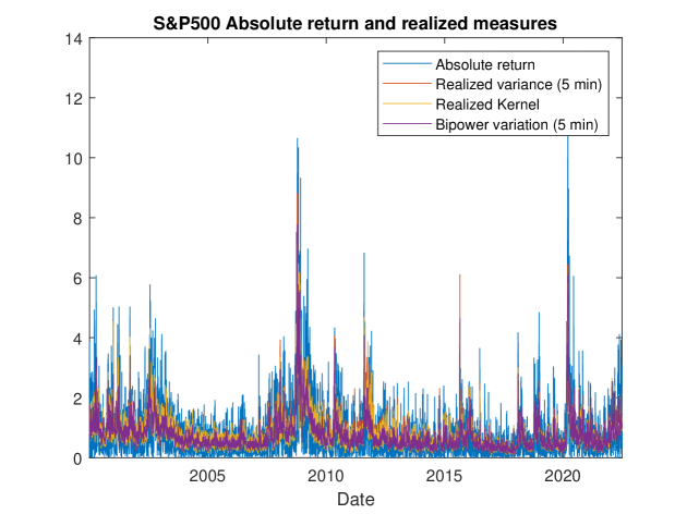
Figure 1: S&P500 absolute return series and three realized measures from January 2000 to June 2022.

Daily, one-step-ahead forecasts of VaR and ES are calculated for the six return series at the $2.5\%$ probability level, in the forecast sample. A rolling window, with fixed in-sample size $T$, is employed to estimate each of $m$ one-step-ahead forecasts of VaR and ES in the forecasting period for each series. Table 2 shows the total sample sizes, plus $T$ and $m$ in each market. $T$ and $m$ differ due to different non-trading days in each market.

Table 2: Summary of the selected data sets and their in-sample and out-of-sample split.

Index	Sample size	In-sample size ($T$)	Out-of-sample size ($m$)
S&P500	5634	3008	2626
FTSE	5667	3020	2647
NASDAQ	5636	3006	2630
HSI	5504	2937	2567
DAX	5697	3050	2647
SMI	5634	3013	2621

5.2 Models in comparison

Table 3 shows the list of 29 models considered in the tail risk forecasting study. As in Section 2, four groups of models, i.e., GARCH, REGARCH, ES-X-CAViaR-X (and its variant ES-CAViaR-X without using the realized measure $x_{t}$ in $\omega_{t}$ of Model (3)), and Realized-ES-CAViaR-X are included, for comparison.

Table 3: A summary of the competing models in the empirical section, based on the model type, realized measures used, and the number of realized measures ($K$).

Model	Type	Realized measures	$K$
GARCH Models
GARCH-t	Parametric	NA	0
EGARCH-t	Parametric	NA	0
GJR-GARCH-t	Parametric	NA	0
GARCH-HS	Semi-Parametric	NA	0
EGARCH-HS	Semi-Parametric	NA	0
GJR-GARCH-HS	Semi-Parametric	NA	0
REGARCH Models
RV5	Parametric	RV5	1
RK	Parametric	RK	1
BV	Parametric	BV	1
RV5-RK	Parametric	RV5, RK	2
RV5-BV	Parametric	RV5, BV	2
RK-BV	Parametric	RK, BV	2
RK-RV5-BV	Parametric	RV5, RK, BV	3
ES-CAViaR-X Models
RV5	Semi-parametric	RV5	1
RK	Semi-parametric	RK	1
BV	Semi-parametric	BV	1
ES-X-CAViaR-X Models
RV5	Semi-parametric	RV5	1
RK	Semi-parametric	RK	1
BV	Semi-parametric	BV	1
Realized-ES-CAViaR Models
RV5	Semi-parametric	RV5	1
RK	Semi-parametric	RK	1
BV	Semi-parametric	BV	1
Realized-ES-CAViaR-M Models
RV5	Semi-parametric	RV5	1
RK	Semi-parametric	RK	1
BV	Semi-parametric	BV	1
RV5-RK	Semi-parametric	RV5, RK	2
RV5-BV	Semi-parametric	RV5, BV	2
RK-BV	Semi-parametric	RK, BV	2
RV5-BV-RK	Semi-parametric	RV5, RK, BV	3

Note: “NA” represents that the model does not use realized measures. Grey shading highlights the proposed models.

Conventional GARCH (Bollerslev, 1986), EGARCH (Nelson, 1991), and GJR-GARCH models (Glosten ., 1993) all with Student’s t return error, parametrically estimated, are included. The two-step QML-HS approach as described in section 2 is also considered, with GARCH, EGARCH and GJR-GARCH employed as the volatility models.

Next, the parametric REGARCH model with RMs: RV5, RK, and BV is considered. Gaussian errors are used for both the return and measurement equations (GG), following Hansen  Huang (2016). A similar MCMC algorithm is employed for estimation of this model. In total, there are seven different versions, being models with one, two or three RMs.

From the semi-parametric field, the ES-CAViaR-X model, ES-X-CAViaR-X models (Gerlach  Wang, 2020) and Realized-ES-CAViaR model ($K=1$) (Wang ., 2023) are included and estimated via similar adaptive MCMC algorthms. Finally, there are seven versions of the proposed Realized-ES-CAViaR-M model included, again being models with one, two or three RMs included.

5.2.1 Assessing Value-at-Risk forecasts

This section discusses evaluation of VaR forecasts. First, the VaR violation rate (VRate) is employed as an informal criterion to assess VaR forecast accuracy. VRate is the proportion of returns in the forecast period that violate or exceed the VaR forecasts $\widehat{Q}_{t}$.

$$\textup{VRate }=\frac{1}{m}\sum_{t=T+1}^{T+m}I(r_{t}<\widehat{Q}_{t})$$ (12)

where $T$ is the in-sample size and $m$ is the forecasting sample size. Models with VRate close to nominal, i.e., $\alpha=2.5\%$, or equivalently $\frac{\textup{VRate}}{\alpha}$ close to 1, are preferred.

Table 4 summarizes the VRates, divided by the nominal $\alpha=2.5\%$, for each model over the six return series. The mean absolute deviation in the “MAD” column employs $2.5\%$ as the target VRate across the six indices. A box indicates the model with ratio of VRate to $\alpha$ closest to one in each market. “Avg Rank” is the average of the ranks across the six markets, calculated by considering the absolute deviation of each VRate from $2.5\%$. The mean absolute values of these deviations (MAD) are presented in the “MAD” column. Blue text represents the 2nd-ranked model in each market.

Table 4 shows that the overall best-ranked models with closest to nominal VRate are the proposed Realized-ES-CAViaR-M models, with single or multiple RMs. All seven models in the proposed Realized-ES-CAViaR-M framework are in the top 10 overall, considering MAD and average rank. Models using BV and RK are consistently highly ranked, compared to those using RV5.

The quantile loss, equation (13), is also used to assess VaR forecast accuracy.

$$\frac{1}{m}\sum_{t=T+1}^{T+m}\left(\alpha-I(r_{t}\leq\widehat{Q}_{t})\right)\left(r_{t}-\widehat{Q}_{t}\right),$$ (13)

where $\widehat{Q}_{T+1},...,\widehat{Q}_{T+m}$ are the quantile forecasts at level $\alpha$. Since the quantile loss function is strictly consistent, the model with minimum sample quantile loss is preferred. Table 5 shows the 2.5% VaR quantile loss function results. The average rank based on the rank of the quantile loss across six markets is also included in the ”Avg Rank“ column.

Based on the average rank, the proposed Realized-ES-CAViaR-M models generally produce lower quantile loss values and are thus typically more accurate in comparison to the other models considered.

First, the parametric REGARCH models, which use the Gaussian return errors and use realized measures, generally have a close performance to the parametric GARCH-t and semi-parametric GARCH-QML type models that do not use the realized measures. This demonstrates the importance of the return error distribution selection in the parametric risk models. The semi-parametric models, which do not require the return error distribution specification, demonstrate an advantage from this aspect.

Second, the ES-CAViaR-X, ES-X-CAViaR-X and Realized-ES-CAViaR models in general generate preferred performance compared to the GARCH and REGARCH type models. This shows the effectiveness of incorporating the realized measures in semi-parametric joint VaR and ES forecasting. The observations are consistent with the ones in Gerlach  Wang (2020) and Wang . (2023).

Lastly, the overall preferred performance of the Realized-ES-CAViaR-M model lends support to the effectiveness of the proposed framework that incorporates the information of multiple realized measures into the the semi-parametric risk forecasting.

5.2.2 Assessing Expected Shortfall forecasts

For the same six series in the forecasting period, the same 29 models are used to generate one-step-ahead forecasts ES on the 2.5% probability level. First, the VaR & ES joint loss function is used to evaluate the ES forecasting accuracy.

As discussed in Section 4.1, Taylor (2019) shows that the negative of the quasi log-likelihood function (9) is strictly consistent for $Q_{t}$ and $\text{ES}_{t}$ considered jointly, and fits into the class of strictly consistent joint loss functions for VaR and ES developed by Fissler  Ziegel (2016). We use the average joint loss $S=\frac{1}{m}\sum_{t=n+1}^{n+m}S_{t}$ to formally and jointly assess and compare the VaR and ES forecasts from all models.

$$S_{t}(r_{t},\widehat{Q}_{t},\widehat{\text{ES}}_{t})=-\text{log}\left(\frac{\alpha-1}{\widehat{\text{ES}}_{t}}\right)-{\frac{(r_{t}-\widehat{Q}_{t})(\alpha-I(r_{t}\leq\widehat{Q}_{t}))}{\alpha\widehat{\text{ES}}_{t}}}.$$ (14)

Table 6 shows the 2.5% VaR and ES joint loss function values for each model and each market. With this measure, the proposed Realized-ES-CAViaR-M model with BV ranks the best overall, followed by the Realized-ES-CAViaR-M models with two realized measures (RV5&BV) and (RK&BV). The proposed framework with all three realized measures ranks the next. Compared to the GARCH, REGARCH and (Realized-)ES-CAViaR type models, the observations are generally consistent with the ones from the quantile loss study.

Lastly, the model confidence set (MCS), introduced by Hansen . (2011), is used to statistically compare the group of models via a loss function with a given confidence level. We use the Matlab code for MCS testing downloaded from Kevin Sheppard’s web page (Sheppard, 2009). The MCS is used to evaluate the statistical significance for both the VaR and ES joint loss (per equation (14) & Table 6) and quantile loss (per equation (13) & Table 5), under the 90% confidence level. Two methods, based on different rules of calculating the test statistic and named R and SQ in the downloaded MCS code, are employed to test the competing models.

Table 7 shows 2.5% VaR and ES joint loss and quantile loss MCS results. The R and SQ methods columns show the total number of times each model is included in the $90\%$ MCS across the six return series (the higher, the better). All the proposed Realized-ES-CAViaR-M models with 1, 2, and 3 RMs are included in the MCS for all six indices. ES-X-CAViaR-X and Realized-ES-CAViaR-X are next best overall, generally being in most, i.e. 4, 5 or 6 MCSs out of 6 markets for both quantile and joint loss. The GARCH, RE-GARCH and ES-CAViaR-X models are typically not included in the joint loss MCS, nor in the quantile loss MCS, in each market.

Overall, across several measures and MCS backtests, for VaR and ES forecasting accuracy comparisons over six markets, the proposed Realized-ES-CAViaR-M model has generally favourable performance, compared to a range of competing models. The performance is marginally most favourable for models using RK and/or BV, compared to those using RV5.

Table 4: $2.5\%$ VaR forecasting $\frac{VRate}{\alpha=2.5\%}$ with different models on six indices.

Model	S&P500	FTSE	NASDAQ	HSI	DAX	SMI	MAD	Avg Rank
GARCH
GARCH-t	1.4318	1.5867	1.5361	1.4647	1.6018	1.3583	1.2414	21.75
EGARCH-t	1.3709	1.4054	1.5057	1.4336	1.3298	1.4040	1.0206	19.08
GJR-GARCH-t	1.2947	1.4809	1.5057	1.3401	1.3298	1.3430	0.9559	17.25
GARCH-QML	1.4928	1.6320	1.6274	1.5115	1.6925	1.4193	1.4065	25.17
EGARCH-QML	1.3557	1.4507	1.5361	1.4492	1.3449	1.3735	1.0459	19.75
GJR-GARCH-QML	1.3861	1.5111	1.5209	1.3245	1.3903	1.3735	1.0443	18.92
REGARCH
RV5	1.8126	1.6169	1.6274	1.4024	1.8587	1.5261	1.6017	26.25
RK	1.7060	1.6471	1.5665	1.3401	1.7832	1.3888	1.4299	23.75
BV	1.7517	1.6169	1.5665	1.3401	0.7556	1.5872	1.2945	20.67
RV5-RK	1.7365	1.6169	1.5665	1.3557	1.8285	1.5261	1.5126	24.83
RV5-BV	1.7060	1.6320	1.5665	1.3401	1.8738	1.5872	1.5440	25.33
RK-BV	1.7060	1.6774	1.5665	1.3401	1.7832	1.6177	1.5379	25.25
RK-RV5-BV	1.6603	1.6169	1.4905	1.4024	1.8285	1.5261	1.4686	23.08
ES-CAViaR-X
RV5	1.2490	1.2845	1.2471	1.0908	1.4507	1.1751	0.6238	15.75
RK	1.1577	1.3147	1.2471	0.9661	1.4356	1.0683	0.5239	12.17
BV	1.1272	1.2694	1.3080	0.9817	1.4205	1.2209	0.5685	13.08
ES-X-CAViaR-X
RV5	1.0206	1.2694	1.1559	1.1063	1.3449	1.0530	0.3959	12.00
RK	1.0510	1.2391	1.0798	1.0596	1.3147	0.9920	0.3134	9.08
BV	1.0358	1.2694	1.0342	1.0284	1.3147	1.0683	0.3128	9.17
Realized-ES-CAViaR
RV5	0.9596	1.2240	1.0951	1.0596	1.3600	1.0836	0.3595	10.17
RK	1.0206	1.1485	1.0342	1.0908	1.3147	1.0072	0.2567	8.00
BV	1.0053	1.2694	1.0038	0.9973	1.2694	1.1141	0.2770	8.67
Realized-ES-CAViaR-M
RV5	0.9596	1.1787	0.9734	1.0908	1.3298	1.0836	0.3125	8.67
RK	0.9901	1.1334	0.9886	1.0596	1.2543	0.9462	0.2177	4.83
BV	0.9901	1.1938	0.9430	1.0440	1.2694	1.0988	0.2804	6.75
RV5-RK	0.9596	1.1636	0.9582	1.0596	1.2694	1.0530	0.2616	5.42
RV5-BV	0.9292	1.1636	0.9582	1.0752	1.2694	1.0988	0.2998	6.58
RK-BV	0.9596	1.2089	0.9582	1.0284	1.2391	1.0378	0.2485	4.42
RV5-BV-RK	0.9292	1.1787	0.9430	1.0440	1.2391	1.0836	0.2805	4.50

Note: Box indicates the favoured models, and the blue text indicates the second-ranked model in each column.

Table 5: $2.5\%$ VaR forecasting quantile loss on six indices.

Model	S&P500	FTSE	NASDAQ	HSI	DAX	SMI	Avg Rank
GARCH
GARCH-t	181.16	183.01	218.51	210.94	225.96	174.99	24.83
EGARCH-t	175.34	176.91	213.38	203.70	217.22	168.55	17.33
GJR-GARCH-t	174.62	176.78	211.11	204.74	219.88	168.00	16.50
GARCH-QML	182.04	183.95	219.82	211.94	227.33	175.39	26.67
EGARCH-QML	176.66	177.88	214.78	204.81	217.64	169.04	19.17
GJR-GARCH-QML	175.54	177.61	212.25	205.42	220.31	168.44	19.33
REGARCH
RV5	183.58	183.32	212.55	202.97	229.64	175.96	25.00
RK	182.07	182.33	212.96	203.85	227.81	175.47	24.83
BV	180.50	181.82	212.06	202.38	264.92	176.93	22.33
RV5-RK	184.07	183.79	213.32	203.10	229.54	174.78	24.67
RV5-BV	181.05	181.41	211.76	203.44	228.82	175.17	22.00
RK-BV	181.74	182.18	211.96	202.94	228.98	177.25	23.17
RV5-RK-BV	181.15	182.09	211.75	203.22	229.52	175.01	22.17
ES-CAViaR-X
RV5	174.63	178.92	205.63	202.98	221.04	172.39	17.67
RK	174.13	178.41	206.84	203.33	222.62	173.16	18.17
BV	173.50	175.28	205.03	202.74	219.76	174.92	14.83
ES-X-CAViaR-X
RV5	169.68	177.18	197.95	200.96	218.75	164.82	11.33
RK	168.21	176.31	197.28	202.40	218.79	166.44	11.17
BV	168.12	174.96	196.17	200.55	219.34	166.18	9.67
Realized-ES-CAViaR
RV5	170.70	178.27	198.02	200.58	218.94	166.60	12.67
RK	171.32	179.02	197.67	201.84	218.60	168.02	13.50
BV	165.76	176.83	196.07	200.91	218.24	167.89	10.00
Realized-ES-CAViaR-M
RV5	165.16	173.09	195.23	198.02	214.70	161.96	4.67
RK	165.32	172.59	195.62	197.93	214.23	163.52	4.67
BV	162.95	171.87	193.95	198.44	214.10	163.10	2.83
RV5-RK	165.58	173.09	194.93	198.23	214.57	162.05	4.83
RV5-BV	163.16	171.86	195.07	198.53	214.30	162.15	3.50
RK-BV	164.08	172.37	194.12	198.19	214.39	163.08	3.67
RV5-BV-RK	163.61	172.35	194.78	198.31	214.46	162.47	3.83

Note: Box indicates the favoured models, and the blue text indicates the second-ranked model in each column. Grey shades the models that are included in the 90% MCS using the R method.

Table 6: $2.5\%$ VaR & ES joint loss function values across six indices.

Model	S&P500	FTSE	NASDAQ	HSI	DAX	SMI	Avg Rank
GARCH
GARCH-t	5274.1	5325.9	5810.0	5641.2	5871.3	5138.3	19.00
EGARCH-t	5187.0	5265.3	5810.0	5553.3	5789.0	5070.5	14.00
GJR-GARCH-t	5207.1	5234.5	5762.1	5565.3	5819.2	5053.7	15.00
GARCH-QML	5373.5	5422.0	5900.4	5701.6	5962.6	5206.3	27.50
EGARCH-QML	5246.3	5314.7	5841.6	5590.7	5824.0	5110.3	17.00
GJR-GARCH-QML	5273.4	5287.6	5811.0	5600.9	5867.4	5097.3	16.00
REGARCH
RV5	5420.3	5436.5	5823.0	5566.9	6133.5	5250.4	29.00
RK	5341.7	5397.8	5837.0	5559.4	6089.0	5239.3	23.00
BV	5367.8	5363.8	5831.9	5552.3	6497.5	5262.3	25.00
RV5-RK	5391.8	5437.6	5855.0	5565.0	6134.5	5233.9	27.50
RV5-BV	5348.5	5361.6	5818.6	5571.2	6090.4	5245.8	23.00
RK-BV	5331.8	5371.2	5832.9	5560.9	6111.8	5273.7	26.00
RV5-RK-BV	5309.0	5386.8	5797.6	5574.1	6106.4	5244.4	21.00
ES-CAViaR-X
RV5	5254.7	5390.9	5668.3	5651.1	6021.1	5270.3	23.00
RK	5219.6	5362.9	5697.3	5613.8	6011.6	5241.6	20.00
BV	5195.1	5302.3	5666.4	5645.3	5961.8	5322.2	18.00
ES-X-CAViaR-X
RV5	4905.8	5146.3	5382.0	5494.9	5748.8	4905.0	12.00
RK	4900.7	5141.0	5380.2	5496.0	5742.2	4951.3	11.00
BV	4900.5	5117.4	5366.6	5491.2	5745.2	4923.0	9.00
Realized-ES-CAViaR
RV5	4908.1	5154.8	5381.6	5482.7	5731.0	4945.1	10.00
RK	4949.7	5159.4	5389.6	5488.7	5724.3	4981.7	13.00
BV	4840.6	5130.4	5366.8	5489.8	5710.1	4959.1	8.00
Realized-ES-CAViaR-M
RV5	4842.7	5085.4	5355.5	5452.8	5681.4	4876.0	6.00
RK	4861.8	5080.6	5359.8	5444.7	5683.9	4899.7	7.00
BV	4810.3	5056.1	5351.6	5451.6	5661.2	4892.0	1.00
RV5-RK	4844.0	5086.0	5351.0	5454.8	5679.0	4871.2	5.00
RV5-BV	4812.7	5054.8	5358.0	5460.4	5664.0	4872.7	2.50
RK-BV	4815.9	5063.0	5345.5	5453.6	5667.9	4884.7	2.50
RV5-BV-RK	4815.9	5063.0	5355.0	5458.2	5670.7	4873.4	4.00

Note: Box indicates the favoured models, and the blue text indicates the second-ranked model in each column.Grey shades the models that are included in the 90% MCS using the R method.

Table 7: 90% model confidence set with R and SQ methods.

Model	Joint Loss		Quantile Loss
	2.5% R	2.5% SQ	2.5% R	2.5% SQ
GARCH
GARCH-t	1	0	1	0
EGARCH-t	2	2	4	2
GJR-GARCH-t	2	1	4	2
GARCH-QML	0	0	1	0
EGARCH-QML	2	1	4	1
GJR-GARCH-QML	1	1	4	1
REGARCH
GG-RV5	1	1	2	1
RK	1	0	2	1
BV	1	1	2	1
RV5-RK	1	1	2	0
RV5-BV	1	1	2	1
RK-BV	1	1	2	0
RV5-RK-BV	0	0	3	0
ES-CAViaR-X
RV5	0	0	4	0
RK	0	0	4	0
BV	0	0	4	2
ES-X-CAViaR-X
RV5	6	4	6	5
RK	5	5	6	4
BV	6	5	6	5
Realized-ES-CAViaR
RV5	6	5	6	4
RK	5	5	6	4
BV	6	5	6	5
Realized-ES-CAViaR-M
RV5	6	6	6	6
RK	6	6	6	6
BV	6	6	6	6
RV5-RK	6	6	6	6
RV5-BV	6	6	6	6
RK-BV	6	6	6	6
RV5-BV-RK	6	6	6	6

6 Conclusion

This paper proposes a new semi-parametric joint VaR and ES forecasting framework incorporating multiple realized measures. The proposed Realized-ES-CAViaR-M models generate highly competitive risk forecasting results regarding quantile loss, VaR and ES joint, and MCS backtest. In particular, the proposed Realized-ES-CAViaR-M models perform improved results compared to their parametric counterpart, e.g., the REGARCH model, and the semi-parametric counterparts, e.g., ES-X-CAViaR-X and Realized-ES-CAViaR.

This work can be improved by considering more realized measures, including their sub-sampled realized measures and different frequencies. Moreover, the proposed framework includes single lags only, which can be extended to multiple lags. Finally, a different version of the model, such as a multiplicative time-varying relationship between VaR and ES via incorporating the information from multiple realized measures, could be considered in future work.

7 Acknowledgement

The authors acknowledge the technical assistance provided by the Sydney Informatics Hub.

References

- Andersen \BBA Bollerslev (\APACyear1998) \APACinsertmetastarandersen1998answering{APACrefauthors}Andersen, T\BPBIG.\BCBT \BBA Bollerslev, T. \APACrefYearMonthDay1998. \BBOQ\APACrefatitleAnswering the skeptics: Yes, standard volatility models do provide accurate forecasts Answering the skeptics: Yes, standard volatility models do provide accurate forecasts.\BBCQ \APACjournalVolNumPagesInternational economic review885–905. \PrintBackRefs\CurrentBib
- Andersen \BOthers. (\APACyear2003) \APACinsertmetastarandersen2003modeling{APACrefauthors}Andersen, T\BPBIG., Bollerslev, T., Diebold, F\BPBIX.\BCBL \BBA Labys, P. \APACrefYearMonthDay2003. \BBOQ\APACrefatitleModeling and forecasting realized volatility Modeling and forecasting realized volatility.\BBCQ \APACjournalVolNumPagesEconometrica712579–625. \PrintBackRefs\CurrentBib
- Artzner \BOthers. (\APACyear1999) \APACinsertmetastarartzner1999coherent{APACrefauthors}Artzner, P., Delbaen, F., Eber, J\BHBIM.\BCBL \BBA Heath, D. \APACrefYearMonthDay1999. \BBOQ\APACrefatitleCoherent measures of risk Coherent measures of risk.\BBCQ \APACjournalVolNumPagesMathematical finance93203–228. \PrintBackRefs\CurrentBib
- Barndorff-Nielsen \BOthers. (\APACyear2009) \APACinsertmetastarbarndorff2009realized{APACrefauthors}Barndorff-Nielsen, O\BPBIE., Hansen, P\BPBIR., Lunde, A.\BCBL \BBA Shephard, N. \APACrefYearMonthDay2009. \APACrefbtitleRealized kernels in practice: Trades and quotes. Realized kernels in practice: Trades and quotes. \APACaddressPublisherOxford University Press Oxford, UK. \PrintBackRefs\CurrentBib
- Barndorff-Nielsen \BBA Shephard (\APACyear2004) \APACinsertmetastarbarndorff2004power{APACrefauthors}Barndorff-Nielsen, O\BPBIE.\BCBT \BBA Shephard, N. \APACrefYearMonthDay2004. \BBOQ\APACrefatitlePower and bipower variation with stochastic volatility and jumps Power and bipower variation with stochastic volatility and jumps.\BBCQ \APACjournalVolNumPagesJournal of financial econometrics211–37. \PrintBackRefs\CurrentBib
- Basel Committee on Banking Supervision (\APACyear2023) \APACinsertmetastarBIS2023{APACrefauthors}Basel Committee on Banking Supervision. \APACrefYear2023. \APACrefbtitleMAR Calculation of RWA for market risk Mar calculation of rwa for market risk. \APACaddressPublisherBank for International Settlements. {APACrefURL} \urlhttps://www.bis.org/bcbs/publ/d457.pdf \PrintBackRefs\CurrentBib
- Bollerslev (\APACyear1986) \APACinsertmetastarbollerslev1986generalized{APACrefauthors}Bollerslev, T. \APACrefYearMonthDay1986. \BBOQ\APACrefatitleGeneralized autoregressive conditional heteroskedasticity Generalized autoregressive conditional heteroskedasticity.\BBCQ \APACjournalVolNumPagesJournal of econometrics313307–327. \PrintBackRefs\CurrentBib
- Chen \BOthers. (\APACyear2022) \APACinsertmetastarchen2022dynamic{APACrefauthors}Chen, W\BPBIY., Peters, G\BPBIW., Gerlach, R\BPBIH.\BCBL \BBA Sisson, S\BPBIA. \APACrefYearMonthDay2022. \BBOQ\APACrefatitleDynamic quantile function models Dynamic quantile function models.\BBCQ \APACjournalVolNumPagesQuantitative Finance2291665–1691. \PrintBackRefs\CurrentBib
- Christensen \BBA Podolskij (\APACyear2007) \APACinsertmetastarchristensen2007realized{APACrefauthors}Christensen, K.\BCBT \BBA Podolskij, M. \APACrefYearMonthDay2007. \BBOQ\APACrefatitleRealized range-based estimation of integrated variance Realized range-based estimation of integrated variance.\BBCQ \APACjournalVolNumPagesJournal of Econometrics1412323–349. \PrintBackRefs\CurrentBib
- Engle (\APACyear1982) \APACinsertmetastarengle1982autoregressive{APACrefauthors}Engle, R\BPBIF. \APACrefYearMonthDay1982. \BBOQ\APACrefatitleAutoregressive conditional heteroscedasticity with estimates of the variance of United Kingdom inflation Autoregressive conditional heteroscedasticity with estimates of the variance of united kingdom inflation.\BBCQ \APACjournalVolNumPagesEconometrica: Journal of the econometric society987–1007. \PrintBackRefs\CurrentBib
- Engle \BBA Manganelli (\APACyear2004) \APACinsertmetastarengle2004caviar{APACrefauthors}Engle, R\BPBIF.\BCBT \BBA Manganelli, S. \APACrefYearMonthDay2004. \BBOQ\APACrefatitleCAViaR: Conditional autoregressive value at risk by regression quantiles Caviar: Conditional autoregressive value at risk by regression quantiles.\BBCQ \APACjournalVolNumPagesJournal of Business & Economic Statistics224367–381. \PrintBackRefs\CurrentBib
- Fissler \BBA Ziegel (\APACyear2016) \APACinsertmetastarfissler2016higher{APACrefauthors}Fissler, T.\BCBT \BBA Ziegel, J\BPBIF. \APACrefYearMonthDay2016. \BBOQ\APACrefatitleHigher order elicitability and Osband’s principle Higher order elicitability and osband’s principle.\BBCQ \APACjournalVolNumPagesThe Annals of Statistics4441680–1707. \PrintBackRefs\CurrentBib
- Francq \BBA Zakoïan (\APACyear2015) \APACinsertmetastarfrancq2015risk{APACrefauthors}Francq, C.\BCBT \BBA Zakoïan, J\BHBIM. \APACrefYearMonthDay2015. \BBOQ\APACrefatitleRisk-parameter estimation in volatility models Risk-parameter estimation in volatility models.\BBCQ \APACjournalVolNumPagesJournal of Econometrics1841158–173. \PrintBackRefs\CurrentBib
- Gao \BBA Song (\APACyear2008) \APACinsertmetastargao2008estimation{APACrefauthors}Gao, F.\BCBT \BBA Song, F. \APACrefYearMonthDay2008. \BBOQ\APACrefatitleEstimation risk in GARCH VaR and ES estimates Estimation risk in garch var and es estimates.\BBCQ \APACjournalVolNumPagesEconometric Theory2451404–1424. \PrintBackRefs\CurrentBib
- Gerlach \BBA Wang (\APACyear2020) \APACinsertmetastargerlach2020semi{APACrefauthors}Gerlach, R.\BCBT \BBA Wang, C. \APACrefYearMonthDay2020. \BBOQ\APACrefatitleSemi-parametric dynamic asymmetric Laplace models for tail risk forecasting, incorporating realized measures Semi-parametric dynamic asymmetric laplace models for tail risk forecasting, incorporating realized measures.\BBCQ \APACjournalVolNumPagesInternational Journal of Forecasting362489–506. \PrintBackRefs\CurrentBib
- Glosten \BOthers. (\APACyear1993) \APACinsertmetastarglosten1993relation{APACrefauthors}Glosten, L\BPBIR., Jagannathan, R.\BCBL \BBA Runkle, D\BPBIE. \APACrefYearMonthDay1993. \BBOQ\APACrefatitleOn the relation between the expected value and the volatility of the nominal excess return on stocks On the relation between the expected value and the volatility of the nominal excess return on stocks.\BBCQ \APACjournalVolNumPagesThe journal of finance4851779–1801. \PrintBackRefs\CurrentBib
- Hansen \BBA Huang (\APACyear2016) \APACinsertmetastarhansen2016exponential{APACrefauthors}Hansen, P\BPBIR.\BCBT \BBA Huang, Z. \APACrefYearMonthDay2016. \BBOQ\APACrefatitleExponential GARCH modelling with realized measures of volatility Exponential garch modelling with realized measures of volatility.\BBCQ \APACjournalVolNumPagesJournal of Business & Economic Statistics342269–287. \PrintBackRefs\CurrentBib
- Hansen \BOthers. (\APACyear2012) \APACinsertmetastarhansen2012realized{APACrefauthors}Hansen, P\BPBIR., Huang, Z.\BCBL \BBA Shek, H\BPBIH. \APACrefYearMonthDay2012. \BBOQ\APACrefatitleRealized GARCH: a joint model for returns and realized measures of volatility Realized garch: a joint model for returns and realized measures of volatility.\BBCQ \APACjournalVolNumPagesJournal of Applied Econometrics276877–906. \PrintBackRefs\CurrentBib
- Hansen \BOthers. (\APACyear2011) \APACinsertmetastarhansen2011model{APACrefauthors}Hansen, P\BPBIR., Lunde, A.\BCBL \BBA Nason, J\BPBIM. \APACrefYearMonthDay2011. \BBOQ\APACrefatitleThe model confidence set The model confidence set.\BBCQ \APACjournalVolNumPagesEconometrica792453–497. \PrintBackRefs\CurrentBib
- Heber \BOthers. (\APACyear2009) \APACinsertmetastarheber2009omi{APACrefauthors}Heber, G., Lunde, A., Shephard, N.\BCBL \BBA Sheppard, K. \APACrefYearMonthDay2009. \BBOQ\APACrefatitleOxford-Man Institute’s realized library, version 0.3 Oxford-man institute’s realized library, version 0.3.\BBCQ \APACjournalVolNumPagesOxford-Man Institute, University of Oxford. \PrintBackRefs\CurrentBib
- Koenker \BBA Machado (\APACyear1999) \APACinsertmetastarkoenker1999goodness{APACrefauthors}Koenker, R.\BCBT \BBA Machado, J\BPBIA. \APACrefYearMonthDay1999. \BBOQ\APACrefatitleGoodness of fit and related inference processes for quantile regression Goodness of fit and related inference processes for quantile regression.\BBCQ \APACjournalVolNumPagesJournal of the American Statistical Association944481296–1310. \PrintBackRefs\CurrentBib
- Martens \BBA Van Dijk (\APACyear2007) \APACinsertmetastarmartens2007measuring{APACrefauthors}Martens, M.\BCBT \BBA Van Dijk, D. \APACrefYearMonthDay2007. \BBOQ\APACrefatitleMeasuring volatility with the realized range Measuring volatility with the realized range.\BBCQ \APACjournalVolNumPagesJournal of Econometrics1381181–207. \PrintBackRefs\CurrentBib
- Nelson (\APACyear1991) \APACinsertmetastarnelson1991conditional{APACrefauthors}Nelson, D\BPBIB. \APACrefYearMonthDay1991. \BBOQ\APACrefatitleConditional heteroskedasticity in asset returns: A new approach Conditional heteroskedasticity in asset returns: A new approach.\BBCQ \APACjournalVolNumPagesEconometrica: Journal of the Econometric Society347–370. \PrintBackRefs\CurrentBib
- Roberts \BOthers. (\APACyear1997) \APACinsertmetastarroberts1997weak{APACrefauthors}Roberts, G\BPBIO., Gelman, A.\BCBL \BBA Gilks, W\BPBIR. \APACrefYearMonthDay1997. \BBOQ\APACrefatitleWeak convergence and optimal scaling of random walk Metropolis algorithms Weak convergence and optimal scaling of random walk metropolis algorithms.\BBCQ \APACjournalVolNumPagesAnnals of Applied probability71110–120. \PrintBackRefs\CurrentBib
- Sheppard (\APACyear2009) \APACinsertmetastarsheppard2009mfe{APACrefauthors}Sheppard, K. \APACrefYearMonthDay2009. \BBOQ\APACrefatitleMFE MATLAB function reference financial econometrics Mfe matlab function reference financial econometrics.\BBCQ \APACjournalVolNumPagesUnpublished paper, Oxford University, Oxford. Available at: http://www. kevinsheppard. com/images/9/95/MFE_Toolbox_Documentation. pdf. \PrintBackRefs\CurrentBib
- Taylor (\APACyear2019) \APACinsertmetastartaylor2019forecasting{APACrefauthors}Taylor, J\BPBIW. \APACrefYearMonthDay2019. \BBOQ\APACrefatitleForecasting value at risk and expected shortfall using a semiparametric approach based on the asymmetric Laplace distribution Forecasting value at risk and expected shortfall using a semiparametric approach based on the asymmetric laplace distribution.\BBCQ \APACjournalVolNumPagesJournal of Business & Economic Statistics371121–133. \PrintBackRefs\CurrentBib
- Wang \BOthers. (\APACyear2023) \APACinsertmetastarwang2023semi{APACrefauthors}Wang, C., Gerlach, R.\BCBL \BBA Chen, Q. \APACrefYearMonthDay2023. \BBOQ\APACrefatitleA semi-parametric conditional autoregressive joint value-at-risk and expected shortfall modeling framework incorporating realized measures A semi-parametric conditional autoregressive joint value-at-risk and expected shortfall modeling framework incorporating realized measures.\BBCQ \APACjournalVolNumPagesQuantitative Finance232309–334. \PrintBackRefs\CurrentBib