When left and right disagree: Entropy and von Neumann algebras in quantum gravity with general AlAdS boundary conditions

Abstract

Euclidean path integrals for UV-completions of $d$-dimensional bulk quantum gravity were recently studied in Colafranceschi:2023urj by assuming that they satisfy axioms of finiteness, reality, continuity, reflection-positivity, and factorization. Sectors ${\cal H}_{\cal B}$ of the resulting Hilbert space were then defined for any $(d-2)$-dimensional surface ${\cal B}$, where ${\cal B}$ may be thought of as the boundary $\partial\Sigma$ of a bulk Cauchy surface in a corresponding Lorentzian description, and where ${\cal B}$ includes the specification of appropriate boundary conditions for bulk fields. Cases where ${\cal B}$ was the disjoint union $B\sqcup B$ of two identical $(d-2)$-dimensional surfaces $B$ were studied in detail and, after the inclusion of finite-dimensional ‘hidden sectors,’ were shown to provide a Hilbert space interpretation of the associated Ryu-Takayanagi entropy. The analysis was performed by constructing type-I von Neumann algebras $\mathcal{A}_{L}^{B},\mathcal{A}_{R}^{B}$ that act respectively at the left and right copy of $B$ in $B\sqcup B$.

Below, we consider the case of general ${\cal B}$, and in particular for ${\cal B}=B_{L}\sqcup B_{R}$ with $B_{L},B_{R}$ distinct. For any $B_{R}$, we find that the von Neumann algebra at $B_{L}$ acting on the off-diagonal Hilbert space sector ${\cal H}_{B_{L}\sqcup B_{R}}$ is a central projection of the corresponding type-I von Neumann algebra on the ‘diagonal’ Hilbert space ${\cal H}_{B_{L}\sqcup B_{L}}$. As a result, the von Neumann algebras $\mathcal{A}_{L}^{B_{L}},\mathcal{A}_{R}^{B_{L}}$ defined in Colafranceschi:2023urj using the diagonal Hilbert space $\mathcal{H}_{B_{L}\sqcup B_{L}}$ turn out to coincide precisely with the analogous algebras defined using the full Hilbert space of the theory (including all sectors $\mathcal{H}_{\mathcal{B}}$). A second implication is that, for any ${\cal H}_{B_{L}\sqcup B_{R}}$, including the same hidden sectors as in the diagonal case again provides a Hilbert space interpretation of the Ryu-Takayanagi entropy. We also show the above central projections to satisfy consistency conditions that lead to a universal central algebra relevant to all choices of $B_{L}$ and $B_{R}$.

1 Introduction

As emphasized in Colafranceschi:2023urj , a number of arguments regarding gravitational entropy that were originally motivated by the AdS/CFT correspondence have now been understood to follow directly from bulk physics. A primary example is the the derivation Almheiri:2019qdq ; Penington:2019kki of the Island Formula for the entropy of Hawking radiation transferred from an asymptotically-locally-AdS (AlAdS) gravitational system to a non-gravitational bath. This derivation simply combines the gravitational path integral arguments of Lewkowycz:2013nqa ; Faulkner:2013ana ; Dong:2016hjy ; Dong:2017xht with the setting studied in Penington:2019npb ; Almheiri:2019psf . And as explained in Marolf:2020rpm , in this context the results may be safely interpreted in terms of standard von Neumann entropies without invoking holography at any intermediate step.

Another class of examples involves taking the semiclassical limit in which Hilbert space densities of states diverge. Using purely bulk methods, one can show that the algebra of observables is generated by a type-II von Neumann factor and its commutant. This observation then leads to an entropy on these algebras that agrees with the quantum-corrected RT formula up to an additive constant Witten:2021unn ; Chandrasekaran:2022eqq ; Penington:2023dql ; Kudler-Flam:2023qfl .

Motivated by such results, it was suggested in Colafranceschi:2023urj that purely bulk arguments (i.e., without assuming the existence of a holographic dual field theory) should suffice to provide a Hilbert-space interpretation of an entropy defined by regions of an AlAdS boundary for which the semiclassical limit is given by the Ryu-Takayangi formula Ryu:2006bv ; Ryu:2006ef (or its covariant Hubeny-Rangamani-Takayanagi generalization Hubeny:2007xt ).

By assuming certain Euclidean-signature axioms, this was then shown to be the case in so-called ‘diagonal’ settings where the boundary $\partial\Sigma$ of a Cauchy surface $\Sigma$ in a corresponding Lorentz-signature spacetime took the form $\partial\Sigma=B\sqcup B$, where $B$ was a compact $(d-2)$-dimensional manifold (with $\partial B=\emptyset$), and on which appropriate boundary conditions were specified for bulk fields.

The argument of Colafranceschi:2023urj was formulated in terms of a supposed path integral for a UV-complete finite-coupling bulk asymptotically-locally-AdS_d (AlAdS_d) theory. The previously-advertised axioms for such path integrals were called finiteness, reality, reflection-positivity, continuity, and factorization. In the above diagonal setting, these properties sufficed to show the associated Hilbert space sectors $\mathcal{H}_{B\sqcup B}$ to be direct sums $\bigoplus_{\mu}\mathcal{H}_{B\sqcup B}^{\mu}$ of Hilbert spaces that factorize as $\mathcal{H}_{B\sqcup B}^{\mu}=\mathcal{H}_{B\sqcup B,L}^{\mu}\otimes\mathcal{H}_{B\sqcup B,R}^{\mu}$, where the left and right factors $\mathcal{H}_{B\sqcup B,L}^{\mu}$ and $\mathcal{H}_{B\sqcup B,R}^{\mu}$ for given $\mu$ are isomorphic but are associated with operator algebras that, in an appropriate sense, act at the respective left and right copy of $B$ in $\mathcal{H}_{B\sqcup B}$. It was then further shown that the path integral defines a trace on such algebras that agrees with the standard sum-over-diagonal-matrix-elements Hilbert-space trace associated with the Hilbert space

$$\undertilde{\cal H}_{B}=\bigoplus_{\mu}{\cal H}_{B\sqcup B,L}^{\mu}\otimes{\mathbb{C}}^{n_{\mu}}=\bigoplus_{\mu}{\cal H}_{B\sqcup B,R}^{\mu}\otimes{\mathbb{C}}^{n_{\mu}}$$ (1)

for appropriate integers $n_{\mu}.$ The corresponding entropies thus agree as well and, by first making use of an appropriate embedding of ${\cal H}_{B\sqcup B}$ in $\undertilde{\mathcal{H}}_{B}\otimes\undertilde{\mathcal{H}}_{B}$ and then connecting with the Lewkowycz-Maldacena argument Lewkowycz:2013nqa and its generalizations, one obtains a Hilbert space interpretation of the Ryu-Takayanagi entropy of either boundary $B$.

The reader should note that the Hilbert space $\undertilde{\cal H}_{B}$ was not explicitly introduced in Colafranceschi:2023urj , though its use will simplify our discussion. Indeed, the tilde decoration at the bottom of $\undertilde{\cal H}_{B}$ is intended to help to distinguish $\undertilde{\cal H}_{B}$ from the various Hilbert spaces defined in Colafranceschi:2023urj that were denoted by symbols with upper tildes. As shown by the 2nd equality in (1), it would be unnatural to assign either an $L$ or an $R$ label to $\undertilde{\cal H}_{B}$. Furthermore, in the diagonal case we can lose nothing by using only a subscript $B$ instead of $B\sqcup B$. This will turn out to be a good choice of notation as we will see below that the same space $\undertilde{\cal H}_{B}$ arises in the analogous analysis of any off-diagaonal sector ${\cal H}_{B\sqcup B^{\prime}}$, where now ${\cal H}_{B\sqcup B^{\prime}}$ is to be embedded in $\undertilde{\cal H}_{B}\otimes\undertilde{\cal H}_{B^{\prime}}$.

The focus of Colafranceschi:2023urj on diagonal sectors $\mathcal{H}_{B\sqcup B}$ had two primary drawbacks. The most obvious was of course that it provided the desired Hilbert space interpretation of RT entropy only when the two boundaries are identical. Directly generalizing the arguments of Colafranceschi:2023urj to the case with $(d-2)$-dimensional boundary $B\sqcup B^{\prime}$ turns out to be nontrivial due to the reliance of Colafranceschi:2023urj on special properties of cylinders $C_{\epsilon}=B\times[0,\epsilon]$. The obstacle is that such cylinders are intrinsically diagonal in the sense that $\partial C_{\epsilon}=B\sqcup B$. We will thus seek other arguments below.

The second issue arises from the fact that the choice of Hilbert space plays a role in the construction of the desired operator algebras. In particular, while an algebra of simple operators can be defined directly using smooth boundary conditions in the path integral, the most useful mathematical structures turn out to be the left and right von Neumann algebras constructed by using a Hilbert space to define an appropriate notion of a completion. While this may seem like a mathematical technicality, it raises the interesting question of whether using the full quantum gravity Hilbert space might lead to von Neumann algebras (and thus to entropies) that differ from the ones constructed using only the diagonal sectors $\mathcal{H}_{B\sqcup B}$ as in Colafranceschi:2023urj .

We will address both of these shortfalls below. As further motivation for our study, it is useful to take inspiration from the AdS/CFT correspondence, in which the bulk path integral is simply equal to a path integral for the dual CFT. While it is not necessarily the most general allowed setting, this case certainly satisfies the axioms of Colafranceschi:2023urj . Furthermore, in the AdS/CFT context, for any choice of $B$ and $B^{\prime}$ we always have the so-called Harlow-factorization property $\mathcal{H}_{B\sqcup B^{\prime}}=\mathcal{H}_{B}\otimes\mathcal{H}_{B^{\prime}}$ so that in particular, the left Hilbert space factor (and the associated type-I von Neumann factor) is manifestly independent of the choice of $B^{\prime}$.

One might then hope that a similar independence of $B^{\prime}$ follows more generally from the axioms of Colafranceschi:2023urj . Below, it will be useful to rename $B,B^{\prime}$ as $B_{L},B_{R}$ and to refer to $B_{L},B_{R}$ as the left and right boundaries. In that notation, while we have already seen in the diagonal context that a given boundary $B_{L}$ is associated with a set of left Hilbert space factors $\mathcal{H}_{B_{L}\sqcup B_{L},L}$, one may nevertheless hope that the full set of such factors has no dependence on $B_{R}$.

As foreshadowed above, this will turn out to be nearly true in the sense that the off-diagonal Hilbert spaces $\mathcal{H}_{B_{L}\sqcup B_{R}}$ again decompose according to

$$\mathcal{H}_{B_{L}\sqcup B_{R}} = \bigoplus_{\mu}\mathcal{H}_{B_{L}\sqcup B_{R}}^{\mu}\ \ \ {\rm with}\ \ \ \mathcal{H}_{B_{L}\sqcup B_{R}}^{\mu}=\mathcal{H}_{B_{L}\sqcup B_{R},L}^{\mu}\otimes\mathcal{H}_{B_{L}\sqcup B_{R},R}^{\mu},$$ (2)

such that every left Hilbert space factor $\mathcal{H}_{B_{L}\sqcup B_{R},L}^{\mu}$ is in fact canonically isomorphic to a left factor $\mathcal{H}_{B_{L}\sqcup B_{L},L}^{\mu}$ associated with the diagonal Hilbert space $\mathcal{H}_{B_{L}\sqcup B_{L}}$. However, for given $B_{R}$ it may be that we find only a subset of the diagonal left Hilbert-space factors $\mathcal{H}_{B_{L}\sqcup B_{L},L}^{\mu}$. Indeed, we will see that there is a natural sense in which the isomorphic factors $\mathcal{H}_{B_{L}\sqcup B_{R},L}^{\mu}$ and $\mathcal{H}_{B_{L}\sqcup B_{L},L}^{\mu}$ can be said to be associated with the same value of $\mu$, so that for any $\mu$ appearing in (2) it is natural to write

$$\mathcal{H}_{B_{L}\sqcup B_{R},L}^{\mu}=\mathcal{H}_{B_{L}\sqcup B_{L},L}^{\mu}=:\mathcal{H}_{B_{L}}^{\mu},$$ (3)

where this defines the symbol $\mathcal{H}_{B_{L}}^{\mu}$ used on the right-hand-side. Here we have refrained from adding an additional _,L subscript on $\mathcal{H}_{B_{L}}^{\mu}$ since the identical Hilbert space arises from the corresponding construction when $B_{L}$ is used as a right boundary (instead of a left boundary as above). In addition, for given $\mu$ the integer $n_{\mu}$ will be shown to be independent of the choice of boundary so that, in the notation of (3), replacing $B$ in (1) by $B_{L},B_{R}$ we may write both

$$\undertilde{\mathcal{H}}_{B_{L}}:=\bigoplus_{\mu}\left(\mathcal{H}_{B_{L}}^{\mu}\otimes{\mathbb{C}}^{n_{\mu}}\right)\ \ \ {\rm and}\ \ \ \undertilde{\mathcal{H}}_{B_{R}}:=\bigoplus_{\mu}\left({\mathcal{H}}_{B_{R}}^{\mu}\otimes{\mathbb{C}}^{n_{\mu}}\right)$$ (4)

for the same integers $n_{\mu}$.

The results of Colafranceschi:2023urj then imply that the trace defined by the path integral on operators that act at any $B_{L}$ or $B_{R}$ coincides with the sum-over-diagonal-matrix-elements trace defined by the Hilbert spaces (4). A Hilbert space interpretation of the Ryu-Takayanagi entropy associated with either $B_{L}$ or $B_{R}$ of states in ${\cal H}_{B_{L}\sqcup B_{R}}$ then follows from an appropriate embedding of ${\cal H}_{B_{L}\sqcup B_{R}}$ in $\undertilde{\cal H}_{B_{L}}\otimes\undertilde{\cal H}_{B_{R}}$.

Finally, we will also verify the analogous statements for the above-mentioned von Neumann algebras, showing in particular that the algebras constructed in Colafranceschi:2023urj using only the diagonal sectors $\mathcal{H}_{B\sqcup B}$ do in fact coincide with von Neumann algebras completed by using the topology defined by the entire quantum gravity Hilbert space. More specficially, we will see that the von Neumann algebra acting at $B_{L}$ associated with an off-diagonal sector $\mathcal{H}_{B_{L}\sqcup B_{R}}$ is always a central projection of the corresponding algebra defined by the diagonal Hilbert space sector $\mathcal{H}_{B_{L}\sqcup B_{L}}$. Furthermore, these projections will be shown to satisfy compatibility conditions that allow us to assemble such central projections into a universal central algebra, independent of the choice of any particular $B_{L}$, from which the central algebra for each pair $B_{L}$,$B_{R}$ can be recovered by acting with an appropriate projection. Such algebraic results are in fact more fundamental than the Hilbert-space results described above and will thus be addressed first in the work below.

This paper is organized as follows. We begin in section 2 by reviewing the construction of algebras and Hilbert spaces from Euclidean path integrals as described in Colafranceschi:2023urj . This includes the definition of general off-diagonal Hilbert space sectors $\mathcal{H}_{B_{L}\sqcup B_{R}}$, as well as algebras $\hat{A}_{L}^{B_{L}\sqcup B_{R}}$, $\hat{A}_{R}^{B_{L}\sqcup B_{R}}$ of operators on $\mathcal{H}_{B_{L}\sqcup B_{R}}$ defined by attaching surfaces respectively to the left and right boundaries $B_{L},B_{R}$. However, these algebras are not complete in any natural topology, and Colafranceschi:2023urj defined von Neumann completions only in the diagonal context $B_{L}=B_{R}$. The new results begin in section 3, which shows that the off-diagonal left-algebra $\hat{A}_{L}^{B_{L}\sqcup B_{R}}$ is canonically identified with a quotient of the diagonal left-algebra $\hat{A}_{L}^{B_{L}\sqcup B_{R}}$, and similarly for the right-algebras. It then remains to study the completions that define the off-diagonal von Neumann algebras in section 4. After developing some useful technology, we demonstrate that the off-diagonal von Neumann algebras are again canonically identified with quotients of the diagonal von Neumann algebras. Section 5 then shows this identification to take the form of a central projection, discusses the relationship between the off-diagonal and diagonal Hilbert spaces, and organizes the discussion of centers in terms of a universal central algebra that is independent of the choices of boundaries. The fact that the left and right von Neumann algebras are commutants on $\mathcal{H}_{B_{L}\sqcup B_{R}}$ is also established in this section by making use of further supporting results from appendix A. With all of the above results in place, it is then straightforward to describe the Hilbert space interpretation of RT entropy in the off-diagonal context. This is done in section 6, after which further discussion and final comments are provided in section 7.

2 Algebras and Hilbert spaces from gravitational path integrals

The results of Colafranceschi:2023urj were established within an axiomatic framework for the Euclidean path integral in UV completions of quantum theories of gravity. The five axioms used in Colafranceschi:2023urj are briefly summarized below, though we refer the reader to Colafranceschi:2023urj for full details and additional discussion.

1. Finiteness: The boundary conditions for the path integral are assumed to form a space $X^{d}$ of $d$-dimensional ‘source manifolds’ $X^{d}$. The path integral then defines a map $\zeta:X^{d}\to\mathbb{C}$ to the complex numbers; i.e., $\zeta(M)$ is well-defined and finite for every $M\in X^{d}$. Local restrictions on the sources may be imposed as needed to achieve this property. As an example, one may choose to require source manifolds to have non-negative scalar curvature.

2. Reality: Let $\underline{X}^{d}$ denote formal finite linear combinations of source manifolds with coefficients in $\mathbb{C}$. We extend $\zeta$ to elements of $\underline{X}^{d}$ by linearity. For every $M\in\underline{X}^{d}$, we have both $M^{*}\in\underline{X}^{d}$ and $[\zeta(M)]^{*}=\zeta(M^{*})$. This axiom is trivial if the original space $X^{d}$ of source manifolds is taken to be real; i.e., if ^∗ is taken to act trivially on $X^{d}$. Furthermore, as noted in the introduction, this axiom also implies a time-reversal symmetry. We thus expect that it can be dropped without significant harm, though we leave such a study for future work.

3. Reflection-Positivity: $\zeta(M)$ is a non-negative real number for reflection-symmetric source manifolds $M$, i.e. $M\in\underline{X}^{d}$ can be written in the form $M=\sum_{I,J=1}^{n}\gamma_{I}^{*}\gamma_{J}M_{I,J}$ where $\gamma_{I}\in\mathbb{C}$, $\gamma_{I}^{*}$ denotes the complex conjugate of $\gamma_{I}$, and where each $M_{I,J}$ can be sliced into two parts $N_{I}^{*}$ and $N_{J}$, for some $n\in\mathbb{Z}^{+}$.

4. Continuity: Suppose that the source manifold $M\in X^{d}$ contains a ‘cylinder’ $C_{\epsilon}$ of the form $B\times[0,\epsilon]$. Then $\zeta$ is continuous in the length $\epsilon$ of this cylinder for all $\epsilon>0$.

5. Factorization: For closed boundary manifolds $M_{1},M_{2}$ and their disjoint union $M_{1}\sqcup M_{2}$, we have $\zeta(M_{1}\sqcup M_{2})=\zeta(M_{1})\zeta(M_{2})$.

The framework can also be applied to contexts like those in Saad:2019lba and Marolf:2020xie where factorization fails, but where the path integral can be expressed as an integral ($\zeta=\int d\alpha\ \zeta_{\alpha}$) over path integrals $\zeta_{\alpha}$ in which all of the above axioms hold. The results of Colafranceschi:2023urj then clearly hold for each $\zeta_{\alpha}$, with corresponding implications for the full path integral $\zeta$.

Another important ingredient in the discussion of Colafranceschi:2023urj was the concept of a source-manifold $N$ with boundary $\partial N$. An operation ^∗ (also used in axiom 3) was defined on $Y_{\mathcal{B}}^{d}$ by complex-conjugating the sources on $N$ and simultaneously reflecting $N$ about its boundary. This ^∗ was then used to define the notion of of a rimmed source-manifold-with-boundary $N$, which is a was allowed to have a non-trivial boundary $\partial N$ so long as some open set containing $\partial N$ was a cylinder of the form $C_{\epsilon}=B\times[0,\epsilon]$ described above with $C_{\epsilon}=C_{\epsilon}^{*}$. We will discuss only boundaries $B$ for which there exist cylinders satisfying this condition.

The space of such rimmed source-manifolds with boundary $\mathcal{B}$ was denoted $Y^{d}_{\mathcal{B}}$. We see that any $N_{1},N_{2}\in Y^{d}_{\mathcal{B}}$ can be naturally sewn together across $\mathcal{B}$ to define a smooth closed source-manifold $M_{N_{1}^{*}N_{2}}$. The space of formal finite linear combinations $\underline{Y}_{\mathcal{B}}^{d}$, equipped with a pre-inner product defined by the path integral of glued source manifolds $\braket{N_{1}}{N_{2}}=\zeta(M_{N_{1}^{*}N_{2}})$, then forms a pre-inner product space which we denote as $H_{\mathcal{B}}$. The Hilbert space $\mathcal{H}_{\mathcal{B}}$ is obtained by first taking the quotient by the space of null vectors $\mathcal{N}_{\mathcal{B}}$, and then taking the completion with respect to the norm. To reflect the fact that it is a dense subspace of $\mathcal{H}_{\mathcal{B}}$, we introduce the notation $\mathcal{D}_{\mathcal{B}}=H_{\mathcal{B}}/\mathcal{N}_{\mathcal{B}}$ for the pre-Hilbert space defined before taking the completion.

The analysis of Colafranceschi:2023urj focused on the case when the boundary ${\mathcal{B}}$ is a disjoint union of two closed boundary manifolds ${\mathcal{B}}=B_{1}\sqcup B_{2}$. The spaces $\underline{Y}^{d}_{B_{1}\sqcup B_{1}}$ and $\underline{Y}^{d}_{B_{2}\sqcup B_{2}}$ can then be promoted to algebras $A_{L}^{B_{1}},A_{R}^{B_{2}}$ by defining products that simply glue together the two surfaces being multiplied. The product $a\cdot_{L}b$ on $\underline{Y}^{d}_{B_{1}\sqcup B_{1}}$ (which is used to define $A_{L}^{B_{1}}$) is defined by gluing the right boundary of $a$ to the left boundary of $b$, while the product $c\cdot_{R}d$ on $\underline{Y}^{d}_{B_{2}\sqcup B_{2}}$ (which is used to define $A_{R}^{B_{2}}$) is defined by gluing the left boundary of $c$ to the right boundary of $d$. Since left and right products are related by $a\cdot_{L}b=b\cdot_{R}a$, we may define $ab:=a\cdot_{L}b=b\cdot_{R}a$. There is also a natural involution $\star$ defined by $a^{\star}:=\left(a^{t}\right)^{*}$, where the transpose operation ^t simply interchanges the labels left and right on the boundaries of $a$. Thus $a^{t}$ is the same source manifold as $a$ but with the left boundary of $a$ now called the right boundary of $a^{t}$, and vice versa.

If we interchange the two boundaries to instead use $\mathcal{B}=B_{2}\sqcup B_{1}$, the same construction defines analogous algebras $A_{L}^{B_{2}}$ and $A_{R}^{B_{1}}$. The involution $\star$ then defines an anti-linear isomorphism between $A^{B_{i}}_{L}$ and $A^{B_{i}}_{R}$. Furthermore, a trace operation $tr$ can be defined on these surface algebras using the path integral, $tr(a):=\zeta(M(a))$, where $M(a)\in\underline{X}^{d}$ denotes the source manifold obtained from gluing together the two copies of $B$ in the boundary of $a\in\underline{Y}^{d}_{B\sqcup B}$.

Representations of the surface algebras $A^{B_{1}}_{L}$ and $A^{B_{2}}_{R}$ on the sector $\mathcal{H}_{B_{1}\sqcup B_{2}}$ were then constructed in two steps. The first step was to consider the natural actions of $A_{L}^{B_{1}},A_{R}^{B_{2}}$ on the pre-inner product space $H_{B_{1}\sqcup B_{2}}$ by gluing the relevant surfaces along corresponding boundary components ($B_{1}$ or $B_{2}$). For example, $a\in A^{B_{1}}_{L}$ is represented by an operator $\hat{a}_{L}$ that acts on $\ket{b}\in H_{B_{1}\sqcup B_{2}}$ by gluing the right boundary of $a$ to the left boundary of $b$ so that $\hat{a}_{L}\ket{b}=\ket{ab}$. The next step used the trace inequality

$$tr(b^{\star}aa^{\star}b)\leq tr(a^{\star}a)tr(b^{\star}b).$$ (5)

derived in Colafranceschi:2023urj for $a$ in either $A^{B_{1}}_{L}$ or $A^{B_{2}}_{R}$ and any $b\in H_{B_{1}\sqcup B_{2}}$. As shown in figure 1, the relation (5) is equivalent to the inequality

$$\langle b|\hat{a}_{L}\hat{a}_{L}^{\dagger}|b\rangle\leq tr(a^{\star}a)\langle b|b\rangle,$$ (6)

which immediately implies that each operator in the representation is bounded. It thus preserves the null space $\mathcal{N}_{B_{1}\sqcup B_{2}}$, and induces a (bounded) operator on $\mathcal{D}_{B_{1}\sqcup B_{2}}$. It follows that there is a unique bounded extension to the Hilbert space $\mathcal{H}_{B_{1}\sqcup B_{2}}$.

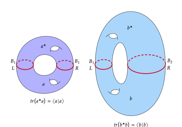
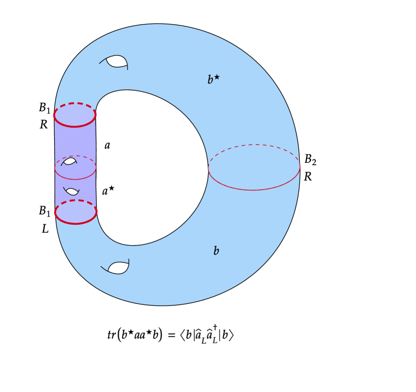
Figure 1: For surfaces $a\in Y^{d}_{B_{L}\sqcup B_{L}}$ and $b\in Y^{d}_{B_{L}\sqcup B_{R}}$, the traces of $a^{\star}a$ and $b^{\star}b$ coincide with $\langle a|a\rangle$ and $\langle b|b\rangle$ as shown in the upper panel. The left hand side $tr(b^{\star}aa^{\star}b)$ of the trace inequality (5) computes the inner product $\langle b|\hat{a}_{L}\hat{a}_{L}^{\dagger}|b\rangle$, as shown in the lower panel.

The left and right representations established on the sector $\mathcal{H}_{B_{1}\sqcup B_{2}}$ are denoted by $\hat{A}^{B_{1}\sqcup B_{2}}_{L}$ and $\hat{A}^{B_{1}\sqcup B_{2}}_{R}$. The adjoint operation defined by $\mathcal{H}_{B_{1}\sqcup B_{2}}$ then satisfies $(\hat{a}_{L})^{\dagger}=\widehat{(a^{\star})}_{L}$, and similarly for the right algebra. Finally, it is clear that operators in $\hat{A}^{B_{1}\sqcup B_{2}}_{L}$ commute with those in $\hat{A}^{B_{1}\sqcup B_{2}}_{R}$.

The remaining analysis of Colafranceschi:2023urj was restricted to so-called diagonal sectors of the form $\mathcal{H}_{B_{1}\sqcup B_{1}}$; i.e., with $B_{1}$ diffeomorphic to $B_{2}$. In that context, left and right von Neumann algebras $\mathcal{A}_{L}^{B_{1}}$ and $\mathcal{A}_{R}^{B_{1}}$ were constructed by taking completions of the representations $\hat{A}_{L}^{{B_{1}}\sqcup{B_{1}}}$ and $\hat{A}_{R}^{{B_{1}}\sqcup{B_{1}}}$ in the weak operator topology. The adjoint operation again acts as an involution on these von Neumann algebras.

A key point was then that the above trace $tr$ can be extended to positive elements of the von Neumann algebras $\mathcal{A}_{L}^{B_{1}}$ and $\mathcal{A}_{R}^{B_{1}}$ by taking it to be defined by

$$tr(a):=\lim_{\beta\downarrow 0}\langle C_{\beta}|a|C_{\beta}\rangle,$$ (7)

where $C_{\beta}$ is an appropriate cylinder of length $\beta$. The result is faithful, normal, and semifinite. In addition, it continues to satisfy the trace inequality (5), as well as related inequalities derived using larger numbers of boundaries. Together, these results require $tr(P)$ to be a non-negative integer for any projection $P$ with finite trace. Each of the algebras $\mathcal{A}^{B_{1}}_{L},\mathcal{A}^{B_{1}}_{R}$ must thus be a direct sum of type I factors. Furthermore, the Hilbert space $\mathcal{H}_{{B_{1}}\sqcup{B_{1}}}$ is a direct sum of Hilbert spaces $\mathcal{H}_{{B_{1}}\sqcup{B_{1}}}^{\mu}$ that factorize as $\mathcal{H}_{{B_{1}}\sqcup{B_{1}}}^{\mu}=\mathcal{H}_{{B_{1}}\sqcup{B_{1}},L}^{\mu}\otimes\mathcal{H}_{{B_{1}}\sqcup{B_{1}},R}^{\mu}$ with $\mathcal{H}_{{B_{1}}\sqcup{B_{1}},L}^{\mu}$ canonically isomorphic to $\mathcal{H}_{{B_{1}}\sqcup{B_{1}},R}^{\mu}$ up to an overall phase. Finally, it was shown that such Hilbert-space factors $\mathcal{H}_{{B_{1}}\sqcup{B_{1}},L}^{\mu}$, $H_{{B_{1}}\sqcup{B_{1}},R}^{\mu}$ could be supplemented with finite dimensional Hilbert spaces ${\mathbb{C}}^{n_{\mu}}$ such that the trace $\widetilde{Tr}$ defined by summing diagonal matrix elements of operators on $\undertilde{\mathcal{H}}_{B_{1}}:=\bigoplus_{\mu}\mathcal{H}_{{B_{1}}\sqcup{B_{1}},L}^{\mu}\otimes{\mathbb{C}}^{n_{\mu}}=\bigoplus_{\mu}\mathcal{H}_{{B_{1}}\sqcup{B_{1}},R}^{\mu}\otimes{\mathbb{C}}^{n_{\mu}}$ coincides on $\mathcal{A}_{L}^{B_{1}}$ and $\mathcal{A}_{R}^{B_{1}}$ with the trace $tr$ defined above. Since $\mathcal{H}_{B_{1}\sqcup B_{1}}\subset\undertilde{\mathcal{H}}_{B_{1}}\otimes\undertilde{\mathcal{H}}_{B_{1}},$ this provided a Hilbert space interpretation of the entropy described by the gravitational replica trick. And by the argument of Lewkowycz:2013nqa , this entropy is well approximated by the Ryu-Takayanagi entropy Ryu:2006bv ; Ryu:2006ef when the bulk theory admits an appropriate semiclassical limit.

3 Off-diagonal representations from the diagonal representation

The main goal of this paper is to generalize the above results to off-diagonal sectors ${\cal H}_{B_{L}\sqcup B_{R}}$ with $B_{L}\neq B_{R}$. We perform the first steps of that analysis in this section, focusing on the surface algebras $A^{B_{L}}_{L}$ and $A^{B_{R}}_{R}$ and their representations $\hat{A}_{L}^{B_{L}\sqcup B_{R}}$ and $\hat{A}_{R}^{B_{L}\sqcup B_{R}}$ on ${\cal H}_{B_{L}\sqcup B_{R}}$. In particular, we will show that any off-diagonal representation $\hat{A}_{L}^{B_{L}\sqcup B_{R}}$ can be identified with a quotient of $\hat{A}_{L}^{B_{L}\sqcup B_{L}}$.

The construction of these objects with $B_{L}\neq B_{R}$ was already given in Colafranceschi:2023urj and was reviewed in section 2. We may thus proceed rapidly. The surface algebras $A^{B_{1}}_{L}$ and $A^{B_{2}}_{R}$ were in fact defined in section 2 using only properties that are intrinsic to the spaces of surfaces $Y^{d}_{B_{1}\sqcup B_{1}},Y^{d}_{B_{2}\sqcup B_{2}}$, without mention of any Hilbert space sector. We thus need only set $B_{1}=B_{L}$ and $B_{2}=B_{R}$ to obtain surface algebras $A^{B_{L}}_{L}$ and $A^{B_{R}}_{R}$ which are identical to those used in the diagonal context.

We will show below that the representation of $A^{B_{L}}_{L}$ on any sector ${\cal H}_{B_{L}\sqcup B_{R}}$ is always a quotient of the representation on the diagonal sector ${\cal H}_{B_{L}\sqcup B_{L}}$, and similarly for the right surface algebra. This statement is equivalent to the claim that, if $n$ lies in the diagonal null space ${\mathfrak{N}}_{L}^{B_{L}\sqcup B_{L}}$ of elements of $A^{B_{L}}_{L}$ that annihilate all states in the diagonal sector ${\cal H}_{B_{L}\sqcup B_{L}}$, then $n$ must also annihilate all states in any non-diagonal sector ${\cal H}_{B_{L}\sqcup B_{R}}$.

To streamline our notation for boundaries, we now introduce the shorthand $LR=B_{L}\sqcup B_{R}$, $LL=B_{L}\sqcup B_{L}$, and $RR=B_{R}\sqcup B_{R}$. We will in particular write $\hat{A}^{LR}_{L}=\hat{A}_{L}^{B_{L}\sqcup B_{R}}$ and $\hat{A}^{LR}_{R}=\hat{A}_{R}^{B_{L}\sqcup B_{R}}$. As in the diagonal case, the adjoint operation defined by $\mathcal{H}_{B_{L}\sqcup B_{R}}$ satisfies $(\hat{a}_{L})^{\dagger}=\widehat{(a^{\star})}_{L}$, and similarly for the right algebra. It is also again clear that operators in $\hat{A}^{LR}_{L}$ commute with those in $\hat{A}^{LR}_{R}$.

The representation $\hat{A}_{L}^{LR}$ is a faithful representation of the quotient algebra $A_{L}^{B_{L}}/{\mathfrak{N}}_{L}^{LR}$, where ${\mathfrak{N}}_{L}^{LR}={\mathfrak{N}}_{L}^{B_{L}\sqcup B_{R}}$ is the null space consisting of elements whose operator representations annihilate the entire sector $\mathcal{H}_{B_{L}\sqcup B_{R}}$. We now make the following claim:

Claim 3.1.

For any $B_{R}$, the null space ${\mathfrak{N}}_{L}^{B_{L}\sqcup B_{R}}$ contains the diagonal null space ${\mathfrak{N}}_{L}^{B_{L}\sqcup B_{L}}$:

$${\mathfrak{N}}_{L}^{B_{L}\sqcup B_{R}}\supseteq{\mathfrak{N}}_{L}^{B_{L}\sqcup B_{L}}.$$ (8)

Here, and throughout the rest of this work, we could of course also discuss the corresponding properties of algebras that act on the right boundary (which here would give ${\mathfrak{N}}_{R}^{B_{L}\sqcup B_{R}}\supseteq{\mathfrak{N}}_{R}^{B_{L}\sqcup B_{L}}$). For simplicity, we will generally refrain from doing so explicitly, though in all cases such properties clearly follow from analogous arguments.

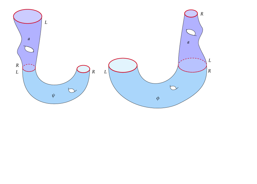
Figure 2: For surfaces $a\in Y^{d}_{LR}$, $\psi\in Y^{d}_{LL}$, $\phi\in Y^{d}_{RR}$, the left panel shows the action of $\hat{a}_{L}$ on $\ket{\psi}\in H_{RR}$ while the right panel shows the action of $\hat{a}_{R}$ on $\ket{\phi}\in H_{LL}$ as defined in equation (9). Both surfaces obtained belong to $Y^{d}_{LR}$.

It is useful to introduce an additional set of bounded operators before we prove claim 3.1. For any surface $a\in Y^{d}_{LR}$, we can define an operator $\hat{a}_{R}:H_{LL}\to H_{LR}$ via the usual gluing of surfaces; see figure 2. This is just the analogue of the action of the surface algebra $A^{B_{L}}_{R}$ on $H_{LL}$, but where the two boundaries of $a$ are now allowed to be different (so that the set of such objects no longer forms a natural algebra, and so that $\hat{a}_{R}|\phi\rangle$ lives in a different Hilbert space sector than the original state $|\phi\rangle$). As usual, the inequality (6) implies that $\hat{a}_{R}$ maps zero-norm states to zero-norm states and so yields a well-defined operator on the image of $H_{LL}$ in $\mathcal{H}_{LL}$. The action of the resulting operator is naturally written in the form

$$\hat{a}_{R}\ket{\phi}=\ket{\phi a}\quad\forall\ket{\phi}\in H_{LL},$$ (9)

where $\phi a$ denotes the surface formed by gluing the right boundary of $\phi\in Y^{d}_{LL}$ to the left boundary of $a\in Y^{d}_{LR}$. The subscript $R$ on $\hat{a}_{R}$ denotes the fact that this operator acts on the right boundary of $\phi$. We also define the analogous left operator $\hat{a}_{L}:H_{RR}\to H_{LR}$ for which

$$\hat{a}_{L}\ket{\psi}=\ket{a\psi}\quad\forall\ket{\psi}\in H_{RR},$$ (10)

Now, as described in section 2, surfaces $a$ define states $\ket{a}$ in the dense subspace $\mathcal{D}_{LR}\subset\mathcal{H}_{LR}$. It will be useful below to think about defining the operator $\hat{a}_{R}$ directly from such $\ket{a}$. To do so, we simply choose an arbitrary representative element $a\in H_{LR}$ of the equivalence class defined by $\ket{a}$. This $a$ is a finite linear combination of surfaces in $Y^{d}_{LR}$ to which we can extend our definition of $\hat{a}_{R}$ by linearity. We then need only observe that if two representatives $a_{1},a_{2}$ differ by some zero-norm surface $N\in{\cal N}_{LR}$, then for any $\phi$ the norm of $\ket{\phi N}$ is given by

$$\langle\phi N|\phi N\rangle=\langle N|\hat{\phi}_{L}^{\dagger}\hat{\phi}_{L}|N\rangle\leq tr(\phi^{\star}\phi)\langle N|N\rangle=0,$$ (11)

where the inequality as usual follows from (6). Thus the operators $\hat{a}_{1,R}$ and $\hat{a}_{2,R}$ are identical so that $\hat{a}_{R}$ is fully defined by the choice of the state $\ket{a}\in\mathcal{D}_{LR}\subset\mathcal{H}_{LR}$.

For later use, we denote the associated map on $\mathcal{D}_{LR}$ by $\Psi_{R}$, and we use $\Psi_{L}$ for the corresponding left operator. In particular, we will use the notation

$$\Psi_{R}(|a\rangle):=\hat{a}_{R},\ \ \ \Psi_{L}(|a\rangle):=\hat{a}_{L},$$ (12)

where we remind the reader that $\hat{a}_{R}$ maps $H_{LL}$ to $H_{LR}$ while $\hat{a}_{L}$ maps $H_{RR}$ to $H_{LR}$.

To discuss the adjoints of $\hat{a}_{R}$ and $\hat{a}_{L}$, we first extend the definition of the $\star$ operation to off-diagonal surfaces:

Definition 1.

For any $a\in Y^{d}_{B_{1}\sqcup B_{2}}$, we define $a^{\star}\in Y^{d}_{B_{2}\sqcup B_{1}}$ to be the source manifold-with-boundary obtained from $a$ by complex-conjugating all sources, relabeling the left boundary $B_{1}$ of $a$ as the right boundary of $a^{\star}$, and similarly relabeling the right boundary $B_{2}$ of $a$ as the left boundary of $a^{\star}$. As shown in figure 3, this definition then satisfies the relation

$$\braket{a}{b}=\zeta(M(a^{\star}b))=tr(a^{\star}b)=tr(ba^{\star})\quad\forall a,b\in H_{B_{1}\sqcup B_{2}},$$ (13)

where the first trace acts on $a^{\star}b\in\underline{Y}^{d}_{B_{2}\sqcup B_{2}}$ and the second trace acts on $ba^{\star}\in\underline{Y}^{d}_{B_{1}\sqcup B_{1}}$.

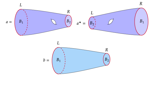
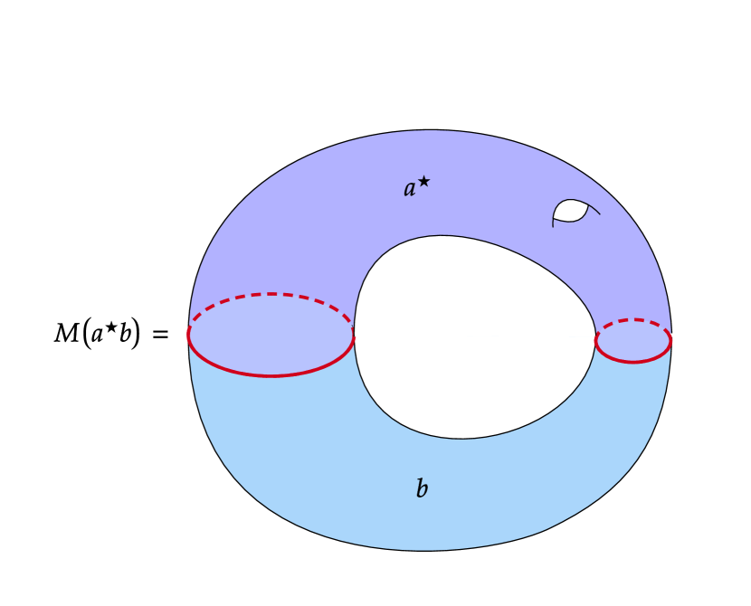
Figure 3: For surfaces $a,b\in Y^{d}_{B_{1}\sqcup B_{2}}$, we can construct $a^{\star}$ and compute $tr(a^{\star}b)$ and $tr(ba^{\star})$. Both are given by evaluating $\zeta$ on the closed surface shown at right, as is $\langle a|b\rangle$ This observation yields (13).

The adjoint $(\hat{a}_{R})^{\dagger}:H_{LR}\to H_{LL}$ of $(\hat{a}_{R})$ is associated with $a^{\star}$ in the sense that it satisfies

$$(\hat{a}_{R})^{\dagger}\ket{\phi}=\ket{\phi a^{\star}}\quad\forall\ket{\phi}\in H_{LR}.$$ (14)

The result (14) can be verified by writing

$$\langle\phi|\psi a\rangle=tr(\phi^{\star}\psi a)=tr(a\phi^{\star}\psi)=tr\left((\phi a^{\star})^{\star}\psi\right)=\langle\phi a^{\star}|\psi\rangle.$$ (15)

As usual, we can use the trace inequality (5) to show that $\hat{a}_{R}$ in fact defines a bounded operator that maps the Hilbert space $\mathcal{H}_{LL}$ to the Hilbert space $\mathcal{H}_{LR}$. In this case we consider again $|\phi\rangle\in H_{LL}$. After setting $b=\phi$, the right analogue of (6) yields

$$\langle\phi|\hat{a}_{R}^{\dagger}\hat{a}_{R}|\phi\rangle\leq\langle\phi|\phi\rangle\langle a|a\rangle.$$ (16)

Thus $\hat{a}_{R}$ annihilates null states in $H_{LL}$ and defines a bounded operator on the dense subspace ${\cal D}_{LL}=H_{LL}/{{\mathcal{N}}}_{LL}\subset\mathcal{H}_{LL}$. A unique bounded extension to $\mathcal{H}_{LL}$ then follows.

As a result, the operation $\Psi_{R}:|a\rangle\mapsto\hat{a}_{R}$ defines a linear map from $\mathcal{D}_{LR}\subset\mathcal{H}_{LR}$ to the space $\mathcal{B}(\mathcal{H}_{LL},\mathcal{H}_{LR})$ of bounded operators from $\mathcal{H}_{LL}$ to $\mathcal{H}_{LR}$. We will extend this map to the entire Hilbert space in section 4.2. In the diagonal context $B_{L}=B_{R}$, the map $\Psi_{R}:H_{LL}\to\hat{A}_{R}^{LL}$ coincides with the representation of the right surface algebra under the natural identification of $H_{LL}$ with $A_{R}^{B_{L}}$.

Returning to claim 3.1, we need to show that any element $a$ of the surface algebra $A_{L}^{B_{L}}$ that is represented by the zero operator on the diagonal Hilbert space $\mathcal{H}_{LL}$ is also represented by zero on any $\mathcal{H}_{LR}$. And since our operators are bounded, it in fact suffices to show that the representation $\hat{a}_{L}\in\hat{A}^{LR}_{L}$ of $a$ on $\mathcal{H}_{LR}$ annihilates every state $|\psi\rangle$ in the dense subspace $\mathcal{D}_{LR}$.

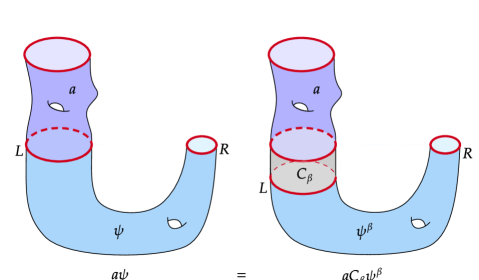
Figure 4: For rimmed surfaces $\psi\in Y^{d}_{LR}$ and $a\in Y^{d}_{LL}$, we define the action of $\hat{a}_{L}$ on $\ket{\psi}$ as $\ket{a\psi}$. As shown in the right panel, we can also separate out a cylinder $C_{\beta}$ from the left rim of $\psi$ and rewrite the surface $a\psi$ as $aC_{\beta}\psi^{\beta}$, where $\psi^{\beta}\in Y^{d}_{LR}$.

Proof.

Let us consider a rimmed surface $\psi\in Y^{d}_{B_{L}\sqcup B_{R}}$ and the corresponding state $|\psi\rangle\in\mathcal{D}_{LR}$. The rim at the left boundary requires there to be a neighborhood of the left boundary whose closure coincides with some cylinder $C_{\beta}$ for some $\beta>0$. As shown in figure 4 we may thus write the surface $a\psi$ as $aC_{\beta}\psi^{\beta}$ for some $\psi^{\beta}\in Y^{d}_{B_{L}\sqcup B_{R}}$. This observation yields the relations

$$\hat{a}_{L}\ket{\psi}=\hat{a}_{L}\ket{C_{\beta}\psi^{\beta}}=\ket{aC_{\beta}\psi^{\beta}}=\hat{\psi}^{\beta}_{R}\ket{aC_{\beta}}=\hat{\psi}_{R}^{\beta}\hat{a}_{L}^{LL}\ket{C_{\beta}}\quad\forall\ket{\psi}\in\mathcal{D}_{LR},$$ (17)

where $\hat{a}_{L}^{LL}$ is the representation of $a$ on the diagonal sector $\mathcal{H}_{LL}$. Thus $\hat{a}_{L}^{LL}=0$ requires $\hat{a}_{L}\ket{\psi}=0$. Since $\mathcal{D}_{LR}$ is the linear span of $|\psi\rangle$ with $\psi\in Y^{d}_{B_{L}\sqcup B_{R}}$, it follows that $\hat{a}_{L}$ annihilates $\mathcal{D}_{LR}$. This establishes ${\mathfrak{N}}_{L}^{LL}\subseteq{\mathfrak{N}}_{L}^{LR}$ as claimed above. ∎

As a result, every left representation $\hat{A}^{LR}_{L}$ of the surface algebra $A_{L}^{B_{L}}$ is also a representation of the diagonal representation $\hat{A}^{LL}_{L}$. This is equivalent to the statement that there is a surjective $*$-homomorphism $\hat{\Phi}_{LR}$ from $\hat{A}^{LL}_{L}$ to any $\hat{A}^{LR}_{L}$. It follows that $\hat{A}^{LR}_{L}$ may be identified with the quotient of $\hat{A}^{LL}_{L}$ by an appropriate kernel, and thus that the diagonal representation contains all information about all representations $\hat{A}^{LR}_{L}$. We will show below that analogous statements continue to hold for the von Neumann algebra completions.

4 Completions and von Neumann algebras

We saw above that, for a given surface algebra $A_{L}^{B_{L}}$, the diagonal representation $\hat{A}^{LL}_{L}$ acts as universal ‘covering algebra’ for any representation $\hat{A}^{LR}_{L}$ in the sense that there is a $*$-homomorphsim $\hat{\Phi}_{LR}$ from $\hat{A}^{LL}_{L}$ to $\hat{A}^{LR}_{L}$. Furthermore, as reviewed in section 2, completing the diagonal representation $\hat{A}^{LL}_{L}$ yields an associated von Neumann algebra $\mathcal{A}_{L}^{B_{L}}$.

We will now generalize this construction to define an off-diagonal von Neumann algebra $\mathcal{A}_{L}^{LR}=\mathcal{A}_{L}^{B_{L}\sqcup B_{R}}$ by completing $\mathcal{A}_{L}^{LR}$ with respect to the weak operator topology on $\mathcal{B}(\mathcal{H}_{B_{L}\sqcup B_{R}})$. It is thus natural to ask if the results of section 3 extend to such completions. To make the notation more uniform between the diagonal and off-diagonal contexts, we will henceforth use the symbol $\mathcal{A}_{L}^{LL}=\mathcal{A}_{L}^{B_{L}\sqcup B_{L}}$ for the von Neumann algebra $\mathcal{A}_{L}^{B_{L}}$ defined using the weak operator topology on the diagonal Hilbert space $\mathcal{H}_{B_{L}\sqcup B_{L}}.$

The goal of this section is to show that this is indeed the case. The subtlety, however, is that the weak operator topology is defined by the Hilbert space on which the operators act. Thus, a priori, two completions might be very different even if we begin with isomorphic representations. It will turn out, however, that our axioms in fact require there to be a simple relation between $\mathcal{A}_{L}^{LR}$ and $\mathcal{A}_{L}^{LL}$.

As a result, we will be able to extend the surjective *-homomorphism $\hat{\Phi}_{LR}:\hat{A}_{L}^{LL}\to\hat{A}_{L}^{LR}$ to a surjective *-homomorphism $\Phi_{LR}:\mathcal{A}_{L}^{LL}\to\mathcal{A}_{L}^{LR}$ that is continuous with respect to the weak operator topology. Note that the extended $\Phi_{LR}$ is written without a hat decoration$\hat{\quad}$. Extending $\hat{\Phi}_{LR}$ means in particular that, given any $a\in\mathcal{A}_{L}^{LL}$, we must construct an appropriate bounded operator $\Phi_{LR}(a)$ on the Hilbert space $\mathcal{H}_{LR}$. This first step will be accomplished in section 4.1, which also verifies that the extension defines a $*$-homomorphism. After an aside to introduce some useful technology in section 4.2, the desired continuity will then be established in section 4.3.

4.1 Extending our homomorphism to the von Neumann algebra $\mathcal{A}_{L}^{LL}$

For each $a$ in the von Neumann algebra $\mathcal{A}_{L}^{LL}$, we will first define the desired $\Phi_{LR}(a)$ as an operator on the dense domain $\mathcal{D}_{LR}$. Any state $|\psi\rangle\in\mathcal{D}_{LR}$ is a finite linear combination

$$\sum_{i=1}^{N}c_{i}|\psi_{i}\rangle$$ (18)

for states $|\psi_{i}\rangle$ defined by rimmed surfaces $\psi_{i}$ with given right and left boundaries. Since each such surface will have a neighborhood of its left boundary that coincides (up to closure) with some cylinder $C_{\epsilon}$ for $\epsilon>0$, by choosing $\epsilon>0$ sufficiently small we can write $\psi_{i}=C_{\epsilon}\psi_{i}^{\epsilon}$ for all $i$; see again figure 4. Defining the state $\ket{\psi^{\epsilon}}=\sum_{i=1}^{N}c_{i}|\psi_{i}^{\epsilon}\rangle$, we may use the associated operator $\hat{\psi}^{\epsilon}_{R}:=\Psi_{R}(|\psi^{\epsilon}\rangle)$ from $\mathcal{H}_{LL}$ to $\mathcal{H}_{LR}$ given by (9). We thus make the following definition for any $a\in\mathcal{A}_{L}^{LL}:$

$$\forall\ket{\psi}\in\mathcal{D}_{LR}\quad{\rm we\ define}\quad\Phi_{LR}(a)\ket{\psi}:=\hat{\psi}_{R}^{\epsilon}a|C_{\epsilon}\rangle\quad{\rm for\ small\ enough}\ \epsilon.$$ (19)

It is manifest that $\Phi_{LR}(a)=\hat{\Phi}_{LR}(a)$ for $a\in\hat{A}^{LR}_{L}$, since then $\hat{\Phi}_{LR}(a)|\psi\rangle=|a\psi\rangle$ and (19) reduces to (9). Furthermore, for all $a$ in the von Neumann algebra $\mathcal{A}_{L}^{LL}$, we will show below that the definition (19) is independent of $\epsilon$ for small enough $\epsilon.$ It is then also manifest that $\Phi_{LR}(ab)=\Phi_{LR}(a)\Phi_{LR}(b)$ and $\Phi_{LR}(\alpha a+\beta b)=\alpha\Phi_{LR}(a)+\beta\Phi_{LR}(b)$ for $\alpha,\beta\in\mathbb{C}$, so that $\Phi_{LR}$ is a homomorphism.

We now establish several claims regarding the definition (19).

Claim 4.1.

The definition (19) is independent of $\epsilon$ so long as $C_{\epsilon}$ is a cylinder common to all rimmed surfaces $\psi_{i}$ appearing in (18).

Proof.

For $a\in\hat{A}_{L}^{LL}$, this claim follows from the observation that $\Phi_{LR}(a)=\hat{\Phi}_{LR}(a)$. Furthermore, a general $a$ in the von Neumann algebra $\mathcal{A}_{L}^{LL}$ can be written as the limit of a net of operators $\{\hat{a}_{\alpha}\}\subset\hat{A}_{L}^{LL}$ that converges to $a$ in the strong operator topology. As a result, since Hilbert spaces are metrizable , given any two common rims $C_{\epsilon}$ and $C_{\delta}$ there must be a sequence $\{\hat{a}_{n}\}\subset\hat{A}_{L}^{LL}$ such that the sequence $\{\hat{a}_{n}|C_{\epsilon}\rangle\}$ converges in norm to $a|C_{\epsilon}\rangle$ while the sequence $\{\hat{a}_{n}|C_{\delta}\rangle\}$ converges in norm to $a|C_{\delta}\rangle$. Since $\hat{\psi}_{R}^{\epsilon}$ and $\hat{\psi}_{R}^{\delta}$ are bounded, we similarly find the limits

$$\hat{\psi}_{R}^{\epsilon}\hat{a}_{n}|C_{\epsilon}\rangle\rightarrow\hat{\psi}_{R}^{\epsilon}a|C_{\epsilon}\rangle$$

$${\rm and}\ \ \ \hat{\psi}_{R}^{\delta}\hat{a}_{n}|C_{\delta}\rangle\rightarrow\hat{\psi}_{R}^{\delta}a|C_{\delta}\rangle.$$ (20)

But since $\hat{a}_{n}\in\hat{A}^{LL}_{L}$ we have $\hat{\psi}_{R}^{\epsilon}\hat{a}_{n}|C_{\epsilon}\rangle=\hat{\Phi}_{LR}(\hat{a}_{n})|\psi\rangle=\hat{\psi}_{R}^{\delta}\hat{a}_{n}|C_{\delta}\rangle$ as noted in the opening sentence of this proof. Thus (4.1) implies $\hat{\psi}_{R}^{\epsilon}a|C_{\epsilon}\rangle=\hat{\psi}_{R}^{\delta}a|C_{\delta}\rangle$ as claimed.

∎

Claim 4.2.

For any $a\in\mathcal{A}_{L}^{LL}$, our $\Phi_{LR}(a)$ is a bounded operator on $\mathcal{D}_{LR}$ (with operator norm no larger than the norm $||a||$ of $a$). It thus admits a unique bounded extension to the entire Hilbert space $\mathcal{H}_{LR}$.

Proof.

We begin by computing the norm of (19). Since $|\psi\rangle\in\mathcal{D}_{LR},$ we have

$$|\Phi_{LR}(a)\ket{\psi}|^{2}=|\hat{\psi}^{\epsilon}_{R}a\ket{C_{\epsilon}}|^{2}=\bra{C_{\epsilon}}a^{\dagger}\hat{\psi}^{\epsilon,\dagger}_{R}\hat{\psi}^{\epsilon}_{R}a\ket{C_{\epsilon}}.$$ (21)

Recall now that $\hat{\psi}^{\epsilon}_{R}$ is a bounded operator from $\mathcal{H}_{LL}$ to $\mathcal{H}_{LR}$. As a result, $\hat{\psi}^{\epsilon,\dagger}_{R}\hat{\psi}^{\epsilon}_{R}$ is a bounded operator on $\mathcal{H}_{LL}$. Furthermore, since $|\psi\rangle$ is of the form (18), the operator $\hat{\psi}^{\epsilon,\dagger}_{R}\hat{\psi}^{\epsilon}_{R}$ is a finite linear combination of the operators $\hat{\psi}^{\epsilon,\dagger}_{i,R}\hat{\psi}^{\epsilon}_{j,R}$, each of which lies in the right representation $\hat{A}^{LL}_{R}$ of the surface algebra $A_{R}^{B_{L}}$. Thus $\hat{\psi}^{\epsilon,\dagger}_{R}\hat{\psi}^{\epsilon}_{R}\in\hat{A}^{LL}_{R}\subset\mathcal{A}_{R}^{LL}$, so that its (unique) positive square root $|\hat{\psi}^{\epsilon}_{R}|$ also lies in the von Neumann algebra $\mathcal{A}_{R}^{LL}$. We may then use the fact that $a$ and $a^{\dagger}$ are in the left von Neumann algebra $\mathcal{A}^{LL}_{L}$ to conclude that they commute with any operator in the right von Neumann algebra $\mathcal{A}_{R}^{LL}$, and in particular with $|\hat{\psi}^{\epsilon}_{R}|$. This observation allows us to write

$$\bra{C_{\epsilon}}a^{\dagger}\hat{\psi}^{\epsilon,\dagger}_{R}\hat{\psi}^{\epsilon}_{R}a\ket{C_{\epsilon}} = \bra{C_{\epsilon}}a^{\dagger}|\hat{\psi}^{\epsilon}_{R}|^{2}a\ket{C_{\epsilon}}=\bra{C_{\epsilon}}|\hat{\psi}^{\epsilon}_{R}|\,a^{\dagger}a\,|\hat{\psi}^{\epsilon}_{R}|\ket{C_{\epsilon}}$$ (22)

$$\leq ||a||^{2}\bra{C_{\epsilon}}|\hat{\psi}^{\epsilon}_{R}|^{2}\ket{C_{\epsilon}}=||a||^{2}\bra{C_{\epsilon}}\hat{\psi}^{\epsilon,\dagger}_{R}\hat{\psi}^{\epsilon}_{R}\ket{C_{\epsilon}}=||a||^{2}\bra{\psi}\psi\rangle,$$ (23)

where $||a||$ is the operator norm of $a$. Thus $\Phi_{LR}(a)$ is bounded as claimed and, in particular, its norm can be no larger than the norm of $a$. ∎

For each $a\in\mathcal{A}_{L}^{LL}$, we may now extend the domain of $\Phi_{LR}(a)$ to all of $\mathcal{H}_{LR}$ by continuity to define $\Phi_{LR}$ as a linear map from $\mathcal{A}_{L}^{LL}$ to the space $\mathcal{B}(\mathcal{H}_{LR})$ of bounded linear operators on $\mathcal{H}_{LR}$. Since bounded operators are determined by their matrix elements on the dense subspace $\mathcal{D}_{LR}$, this extension is again a homomorphism. One can also quickly use (19) (and the fact that $a\in\mathcal{A}_{L}^{LL}$ commutes with $\hat{\psi}^{\epsilon,\dagger}_{1,R}\hat{\psi}^{\epsilon}_{2,R}\in\mathcal{A}_{R}^{LL}$ for any $|\psi_{1}\rangle,|\psi_{2}\rangle\in\mathcal{D}_{LR}$) to show that $\Phi_{LR}$ is a $*$-homomorphism, meaning that $\Phi_{LR}(a^{\dagger})=\left(\Phi_{LR}(a)\right)^{\dagger}$. We will also mention that we will find in section 4.3 that $\Phi_{LR}(a)$ is continuous with respect to the weak operator topology. Since we know that $\Phi_{LR}$ maps $\hat{A}_{L}^{LL}\subset\mathcal{A}_{L}^{LL}$ onto $\hat{A}_{L}^{LR}$, and since the $\mathcal{A}_{L}^{LR}$ is the closure of $\hat{A}_{L}^{LR}$ in the weak operator topology, it will then follow that $\Phi_{LR}:\mathcal{A}_{L}^{LL}\rightarrow A_{L}^{LR}$ is a surjective $*$-homomorphism. This is precisely the analogue of our result from section 3 at the level of the von Neumann algebras $A_{L}^{LL},A_{L}^{LR}$.

4.2 Vectors in an off-diagonal sector as intertwining operators

Before proceeding to the proof of continuity in section 4.3, it will be useful to first derive some additional properties of the map $\Psi_{R}$. Recall that section 3 defined $\Psi_{R}$ as a linear map from $\mathcal{D}_{LR}$ to $\mathcal{B}(\mathcal{H}_{LL},\mathcal{H}_{LR})$. The results of section 4.1 will turn out to imply this $\Psi_{R}$ to be continuous in the strong operator topology. In particular, we now establish the following claim:

Claim 4.3.

The map $\Psi_{R}:\mathcal{D}_{LR}\to\mathcal{B}(\mathcal{H}_{LL},\mathcal{H}_{LR})$ is continuous w.r.t. the norm topology on $\mathcal{H}_{LR}$ and the strong operator topology on $\mathcal{B}(\mathcal{H}_{LL},\mathcal{H}_{LR})$. It then follows that $\Psi_{R}$ admits a unique continuous extension to the entire Hilbert space.

Proof.

Since $\mathcal{D}_{LR}$ is a metric space, the map $\Psi_{R}$ is continuous if and only if it acts continuously on preserves all convergent sequences. Consider then an arbitrary sequence of vectors $\{\ket{\psi_{n}}\}\subset\mathcal{D}_{LR}$ that converges to some $|\psi\rangle\in\mathcal{H}_{LR}$. The first step is to show that the corresponding sequence of operators $\{\widehat{\psi_{n}}_{R}=\Psi_{R}(\ket{\psi_{n}})\}$ is uniformly bounded. In particular, replacing $|a\rangle$ by $|\psi_{n}\rangle$ in (16) shows that $||\widehat{\psi_{n}}_{R}||$ is bounded by $\sqrt{\braket{\psi_{n}}{\psi_{n}}}$. In addition, since the sequence $\{\ket{\psi_{n}}\}$ converges in $\mathcal{H}_{LR}$, we know the sequence of norms $\{\braket{\psi_{n}}{\psi_{n}}\}$ is convergent and must be bounded. The sequence of operator norms $\{||\hat{\psi}_{n}||\}$ is thus bounded as well, so that the sequence $\{\hat{\psi}_{n}\}$ is uniformly bounded.

Next, for any $\ket{x}\in\mathcal{D}_{LL}$ we will show that the sequence of vectors $\{\widehat{\psi_{n}}_{R}\ket{x}\}$ converges in $\mathcal{H}_{LR}$. Let us first note that (9) implies

$$\widehat{\psi_{n}}_{R}\ket{x}=\ket{x\psi_{n}}=\hat{\Phi}_{LR}(\hat{x}_{L})\ket{\psi_{n}},$$ (24)

where $x\in H_{LL}$ is any representative of the vector $\ket{x}$, and where $\hat{x}_{L}:=\Psi_{L}(\ket{x})\in\hat{A}_{L}^{LL}$ is the bounded operator associated with the representation of $x\in A_{L}^{B_{L}}$ on the diagonal sector $\mathcal{H}_{LL}$. Since the sequence of vectors $\ket{\psi_{n}}$ converges to $|\psi\rangle$, and since $\hat{\Phi}_{LR}(\hat{x}_{L})$ is bounded, (24) shows that the sequence of vectors $\widehat{\psi_{n}}_{R}\ket{x}$ also converges to $\hat{\Phi}_{LR}(\hat{x}_{L})|\psi\rangle$.

Via a standard calculation, it then follows that, given any Cauchy sequence $\{|x_{n}\rangle\}\subset\mathcal{D}_{LR}$, the sequence $\widehat{\psi_{n}}_{R}|x_{n}\rangle$ is also Cauchy, and that it thus converges in $\mathcal{H}_{LR}$ (see e.g. theorem 6 in section 15.2 of Lax ). This means that the sequence of operators $\widehat{\psi_{n}}_{R}$ converges in the strong operator topology to an operator $\hat{\psi}_{R}$. In particular, for any $|\psi\rangle\in\mathcal{H}_{LR}$, the limit yields a bounded operator $\hat{\psi}_{R}$ satisfying

$$\forall\ket{x}\in\mathcal{D}_{LL},\quad\hat{\psi}_{R}\ket{x}=\hat{\Phi}_{LR}(\hat{x}_{L})\ket{\psi}.$$ (25)

We may thus define $\Psi_{R}(|\psi\rangle):=\hat{\psi}_{R}$. ∎

We will now show the extended $\Psi_{R}$ to satisfy the following extension of (9).

Claim 4.4.

$\forall\ket{\psi}\in\mathcal{H}_{LR}$, the operator $\hat{\psi}_{R}=\Psi_{R}(\ket{\psi}):\mathcal{H}_{LL}\to\mathcal{H}_{LR}$ is an intertwining operator between the von Neumann algebras $\mathcal{A}_{L}^{LL}$ and $\mathcal{A}_{L}^{LR}$. Specifically, we have

$$\Phi_{LR}(a)\hat{\psi}_{R}=\hat{\psi}_{R}a\quad\forall a\in\mathcal{A}^{LL}_{L}.$$ (26)

Proof.

Any $\ket{\psi}\in\mathcal{H}_{LR}$ is the Hilbert space limit of a sequence $\{\ket{\psi_{n}}\}\subset\mathcal{D}_{LR}$. Note that for any $\epsilon>0$ we may construct the states $\ket{\phi_{n}}:=\ket{C_{\epsilon}\psi_{n}}\in\mathcal{D}_{LR}$, and that $\widehat{\phi_{n}}_{R}^{\epsilon}=\widehat{\psi_{n}}_{R}$. For any $a\in\mathcal{A}_{L}^{LL}$ we may thus write

$$\Phi_{LR}(a)\widehat{\psi_{n}}_{R}|C_{\epsilon}\rangle=\Phi_{LR}(a)|C_{\epsilon}\psi_{n}\rangle=\widehat{\psi_{n}}_{R}a|C_{\epsilon}\rangle,$$ (27)

where the first equality is the definition of $\widehat{\psi_{n}}_{R}$ and the second is a direct application of (19). Recalling that $\widehat{\psi_{n}}_{R}=\Psi_{R}(|\psi_{n}\rangle)$, and that $\hat{\psi}_{R}=\Psi_{R}(|\psi\rangle)$, boundedness of $\Phi_{LR}(a)$ and the continuity property of Claim 4.3 allow us to take the limit $n\rightarrow\infty$ to find

$$\Phi_{LR}(a)\hat{\psi}_{R}|C_{\epsilon}\rangle=\hat{\psi}_{R}a|C_{\epsilon}\rangle.$$ (28)

To show that the above intertwining relation in fact holds when acting on arbitrary states in $\mathcal{H}_{LL}$, we simply consider any $\kappa\in\underline{Y}_{LL}^{d}$ and compute

$$\hat{\psi}_{R}a|\kappa C_{\epsilon}\rangle=\hat{\psi}_{R}a\hat{\kappa}_{L}|C_{\epsilon}\rangle = \Phi_{LR}(a\hat{\kappa}_{L})\hat{\psi}_{R}|C_{\epsilon}\rangle$$ (29)

$$= \Phi_{LR}(a)\Phi_{LR}(\hat{\kappa}_{L})\hat{\psi}_{R}|C_{\epsilon}\rangle$$ (30)

$$= \Phi_{LR}(a)\hat{\psi}_{R}\hat{\kappa}_{L}|C_{\epsilon}\rangle=\Phi_{LR}(a)\hat{\psi}_{R}|\kappa C_{\epsilon}\rangle.$$ (31)

Here the last equality on the first line uses (28) with the $a$ of (28) replaced by $a\hat{\kappa}_{L}$. We then pass to the second line using the fact that $\Phi_{LR}$ is a homomorphism as shown at the end of section 4.1. The third line follows by applying (28) with with the $a$ of (28) replaced by $\hat{\kappa}_{L}$. Since the operators $\hat{\phi}_{R},a,\Phi_{LR}(a)$ are bounded, and since every state in the dense subspace $\mathcal{D}_{LR}\subset\mathcal{H}_{LR}$ is of the form $|\kappa C_{\epsilon}\rangle$ for some $\kappa,\epsilon$, the general result (26) follows by taking corresponding limits of (29). ∎

Before proceeding to the next section, we also wish to establish a further useful property of the extended map $\Psi_{R}$. This property is a partial extension of (13) associated with the fact that $\hat{\psi}^{\dagger}_{R}\hat{\psi}_{R}$ lies in $\mathcal{A}_{R}^{LL}$. In particular, we will find

$$tr(\hat{\psi}^{\dagger}_{R}\hat{\psi}_{R})=\braket{\psi}{\psi}\quad\forall\ket{\psi}\in\mathcal{H}_{LR}.$$ (32)

To see this, we will use the following two results:

Claim 4.5.

For cylinder operators $\widehat{C_{\beta}}_{L}\in\hat{A}_{L}^{LL}$, the limit $\lim_{\beta\downarrow 0}\Phi_{LR}(\widehat{C_{\beta}}_{L})$ converges in the strong operator topology to the identity ${\mathds{1}}\in B(\mathcal{H}_{LR})$.

Proof.

Since $\widehat{C_{\beta}}_{L}$ is the representation of the cylinder $C_{\beta}$ on $\mathcal{H}_{LL}$, we know from section 3 that $\Phi_{LR}(\widehat{C_{\beta}}_{L})$ is just the corresponding representation of $C_{\beta}$ on the off-diagonal Hilbert space $\mathcal{H}_{LR}$. Furthermore, from claim (16) we have $||\Phi_{LR}(\widehat{C_{\beta}}_{L})||\leq||\widehat{C_{\beta}}_{L}||$. And since it was shown in appendix A of Colafranceschi:2023urj that $||\hat{C}_{\beta}||\to 1$ as $\beta\downarrow 0$, the operators $\Phi_{LR}(\widehat{C_{\beta}}_{L})$ are uniformly bounded at small $\beta$. We also observe that, since states in $\mathcal{H}_{LR}$ are determined by their inner products with states in $\mathcal{D}_{LR}$, for any $\ket{x}\in\mathcal{D}_{LR}$ the continuity axiom of Colafranceschi:2023urj requires the vectors $\Phi_{LR}(\widehat{C_{\beta}}_{L})\ket{x}=\ket{C_{\beta}x}$ to converge to $\ket{x}$ in the limit $\beta\downarrow 0$. Together, as in the proof of claim 4.3, these properties imply that $\Phi_{LR}(\widehat{C_{\beta}}_{L})$ converges in the strong operator topology to ${\mathds{1}}$ as $\beta\downarrow 0$; see e.g. theorem 15.2.6 of Lax . ∎

Claim 4.6.

For any $|\psi\rangle\in{\cal H}_{B_{1}\sqcup B_{2}}$, we have

$$|\psi\rangle=\lim_{\beta\downarrow 0}\hat{\psi}_{R}|C_{\beta}\rangle$$ (33)

for $C_{\beta}$ the cylinder of length $\beta$ with boundary $B_{1}\sqcup B_{1}$.

Proof.

Since any such state $|\psi\rangle$ is fully determined by its inner products with states in $\mathcal{D}_{B_{1}\sqcup B_{2}}$, is clear from the continuity axiom that (33) holds for $|\psi\rangle\in\mathcal{D}_{B_{1}\sqcup B_{2}}$. For more general $|\psi\rangle$, we may consider a sequence of states $|\psi_{n}\rangle\in\mathcal{D}_{B_{1}\sqcup B_{2}}$ that converge to $|\psi\rangle.$ Continuity of $\Psi_{R}$ and boundedness of each operator $\widehat{\left(C_{\beta}\right)}_{L}$ then gives

$$\lim_{\beta\downarrow 0}\hat{\psi}_{R}|C_{\beta}\rangle = \lim_{\beta\downarrow 0}\lim_{n\rightarrow\infty}\widehat{\left(\psi_{n}\right)}_{R}|C_{\beta}\rangle$$ (34)

$$= \lim_{\beta\downarrow 0}\lim_{n\rightarrow\infty}\hat{\Phi}_{LR}\left(\widehat{\left(C_{\beta}\right)}_{L}\right)|\psi_{n}\rangle$$ (35)

$$= \lim_{\beta\downarrow 0}\hat{\Phi}_{LR}\left(\widehat{\left(C_{\beta}\right)}_{L}\right)|\psi\rangle=|\psi\rangle,$$ (36)

where we pass from the first to the second line using (25), and where the final step uses claim 4.5. ∎

Equation (32) then follows from (33) by applying definition (7) of the trace on positive elements of $\mathcal{A}_{R}^{LL}$.

4.3 Continuity of $\Phi_{LR}$ in the weak operator topology

The goal of this section is to show that our $*$-homomorphism $\Phi_{LR}$ is continuous with respect to the weak operator topology (imposed on both $\mathcal{B}(\mathcal{H}_{LL})$ and $\mathcal{B}(\mathcal{H}_{LR})$). In order to do so, we first establish the following intermediate claim.

Claim 4.7.

For any $\ket{\gamma}\in\mathcal{H}_{LR}$ and any $a\in\mathcal{A}_{L}^{LL}$, we have

$$\quad\braket{\gamma}{\Phi_{LR}(a)}{\gamma}=\braket{\gamma_{LL}}{a}{\gamma_{LL}},\quad$$ (37)

where we have defined $|\gamma_{LL}\rangle:=\lim_{\beta\downarrow 0}|\hat{\gamma}_{R}||C_{\beta}\rangle\in\mathcal{H}_{LL}$ and where $|\hat{\gamma}_{R}|$ is the positive square root of $\hat{\gamma}^{\dagger}_{R}\hat{\gamma}_{R}$.

Proof.

Let us first rewrite $\braket{\gamma}{\Phi_{LR}(a)}{\gamma}$ by inserting the identity operator in the form $\lim_{\beta\downarrow 0}\Phi_{LR}(\widehat{C_{\beta}}_{L})$ established in claim 4.5. As noted in the proof of that claim, if $\widehat{C_{\beta}}_{L}$ is a cylinder operator on $\mathcal{H}_{LL}$, then $\hat{\Phi}_{LR}(\widehat{C_{\beta}}_{L})$ is the corresponding cylinder operator on $\mathcal{H}_{LR}$. We thus have

$$\braket{\gamma}{\Phi_{LR}(a)}{\gamma}=\lim_{\beta\downarrow 0}\braket{\gamma}{\Phi_{LR}(a)\Phi_{LR}(\widehat{C_{\beta}}_{L})}{\gamma}=\lim_{\beta\downarrow 0}\braket{\gamma}{\Phi(a)\hat{\gamma}_{R}}{C_{\beta}}=\lim_{\beta\downarrow 0}\braket{\gamma}{\hat{\gamma}_{R}a}{C_{\beta}}$$ (38)

where in the second equality we have used equation (25) with $|\psi\rangle=|\gamma\rangle$ and $|x\rangle=|C_{\beta}\rangle$, and where the third equality used (26) (again with $|\psi\rangle=|\gamma\rangle$).

We now insert another identity operator and perform similar manipulations to write

$$\hat{\gamma}_{R}^{\dagger}\ket{\gamma}=\lim_{\epsilon\downarrow 0}\hat{\gamma}_{R}^{\dagger}\Phi_{LR}(\widehat{C_{\epsilon}}_{L})\ket{\gamma}=\lim_{\epsilon\downarrow 0}\hat{\gamma}_{R}^{\dagger}\hat{\gamma}_{R}\ket{C_{\epsilon}}=\lim_{\epsilon\downarrow 0}|\hat{\gamma}_{R}|^{2}\ket{C_{\epsilon}}.$$ (39)

Since $tr(|\hat{\gamma}_{R}|^{2})=tr(\hat{\gamma}_{R}^{\dagger}\hat{\gamma}_{R})=\braket{\gamma}{\gamma}$ is finite, Corollary 1 of Colafranceschi:2023urj then shows that the limit of $|\hat{\gamma}_{R}||C_{\epsilon}\rangle$ converges as $\epsilon\downarrow 0$ to a state $|\gamma_{LL}\rangle\in\mathcal{H}_{LL}$. Thus (39) yields

$$\hat{\gamma}_{R}^{\dagger}\ket{\gamma}=|\hat{\gamma}_{R}|\ |\gamma_{LL}\rangle$$ (40)

and we may evaluate (38) by writing

$$\lim_{\beta\downarrow 0}\braket{\gamma}{\hat{\gamma}_{R}a}{C_{\beta}}=\lim_{\beta\downarrow 0}\braket{\gamma_{LL}}{\ }{\hat{\gamma}_{R}|a\ |C_{\beta}}=\lim_{\beta\downarrow 0}\braket{\gamma_{LL}}{\ a}{\hat{\gamma}_{R}|\ |C_{\beta}}=\braket{\gamma_{LL}}{a}{\gamma_{LL}},$$ (41)

where the second step follows by noting that $|\hat{\gamma}_{R}|$ lies in the right von Neumann algebra $\mathcal{A}_{R}^{LL}$ and so necessarily commutes with $a\in\mathcal{A}_{L}^{LL}$. Combining (41) with (38) then completes the desired proof. ∎

We have now acquired all of the tools we need to prove continuity of the map $\Phi_{LR}$ in the weak operator topology. Recall that convergence in the weak operator topology of the net of operators $\{\mathcal{O}_{\alpha}\}$ on a Hilbert space $\mathcal{H}$ is equivalent to convergence of the associated nets of matrix elements $\{\langle\phi_{1}|\mathcal{O}_{\alpha}|\phi_{2}\rangle\}$ for all $|\phi_{1}\rangle,|\phi_{2}\rangle\in\mathcal{H}$. In particular, let us consider any state $|\gamma\rangle\in\mathcal{H}_{LR}$ and the associated state $|\gamma_{LL}\rangle\in\mathcal{H}_{LL}$ defined as in Claim 4.7. If a net of operators $\{a_{\alpha}\}\subset\mathcal{A}^{LL}_{L}$ converges in the weak operator topology to $b\in\mathcal{A}^{LL}_{L}$, then the net of expectation values $\{\braket{\gamma_{LL}}{a_{\alpha}}{\gamma_{LL}}\}$ clearly converges to $\braket{\gamma_{LL}}{b}{\gamma_{LL}}$. Claim 4.7 then implies that the net of expectation values $\{\braket{\gamma}{\Phi_{LR}(a_{\alpha})}{\gamma}\}$ also converges to $\{\braket{\gamma}{\Phi_{LR}(b)}{\gamma}\}$.

Using the standard construction of general matrix elements from expectation values, this is enough to establish that the net of matrix elements $\{\langle\phi_{1}|\Phi_{LR}(a_{\alpha})|\phi_{2}\rangle\}$ also converges to $\langle\phi_{1}|\Phi_{LR}(b)|\phi_{2}\rangle.$ In particular, given any two states $\ket{\phi_{1}},\ket{\phi_{2}}$, we can define $\ket{\alpha}=\ket{\phi_{1}}+\ket{\phi_{2}}$ and $\ket{\beta}=\ket{\phi_{2}}+i\ket{\phi_{1}}$ to write (for any operator $a$)

$$\braket{\phi_{1}}{a}{\phi_{2}}=(\braket{\alpha}{a}{\alpha}+i\braket{\beta}{a}{\beta})/2-\braket{\phi_{1}}{a}{\phi_{1}}-\braket{\phi_{2}}{a}{\phi_{2}}.$$ (42)

Convergence of expectation values of a net of operators thus implies convergence of all matrix elements. In particular, we see from the above that the net $\{\Phi_{LR}(a_{\alpha})\}$ converges to $\Phi_{LR}(b)$ in the weak operator topology.

We thus see that $\Phi_{LR}$ is continuous in the weak operator topology. This fact can be used to provide an alternate proof that $\Phi_{LR}$ is a $*$-homomorphism directly from the corresponding properties of the map $\hat{\Phi}_{LR}:\hat{A}_{L}^{LL}\rightarrow\hat{A}_{L}^{LR}$. And since the von Neumann algebras $\mathcal{A}_{L}^{LL},\mathcal{A}_{L}^{LR}$ are the weak-operator-topology closures of $\hat{A}_{L}^{LL},\hat{A}_{L}^{LR}$, surjectivity of $\hat{\Phi}_{LR}:\hat{A}_{L}^{LL}\rightarrow\hat{A}_{L}^{LR}$ implies surjectivity of $\Phi_{LR}:\mathcal{A}_{L}^{LL}\rightarrow\mathcal{A}_{L}^{LR}$. As a result, the off-diagonal von Neumann algebra $\mathcal{A}_{L}^{LR}$ is isomorphic to the quotient $\mathcal{A}_{L}^{LL}/\ker(\Phi_{LR})$. This establishes analogues of the results of section 3 at the level of the corresponding von Neumann algebras.

Furthermore, since distinct sectors $\mathcal{H}_{\mathcal{B}}$ are orthogonal, the above observations achieve our primary goal. In particular, they show agreement between the von Neumann algebra $\mathcal{A}_{L}^{LL}=\mathcal{A}_{L}^{B_{L}\sqcup B_{L}}$ (defined from the surface algebra $A_{L}^{B_{L}}$ by the diagonal sector $\mathcal{H}_{LL}=\mathcal{H}_{B_{L}\sqcup B_{L}}$) and the von Neumann algebra defined by using the representation of same surface algebra $A_{L}^{B_{L}}$ on the larger Hilbert space

$${\mathbb{H}}_{B_{L}}:=\oplus_{B_{R}}\mathcal{H}_{B_{L}\sqcup B_{R}}.$$ (43)

Here the sum on the right is over all possible right boundaries $B_{R}$ (including the empty set). This is the largest Hilbert space defined by the Euclidean path integral on which $A_{L}^{B_{L}}$ can naturally be said to act. In this sense the von Neumann algebra $\mathcal{A}_{L}^{LL}=\mathcal{A}_{L}^{B_{L}\sqcup B_{L}}$ defined by the diagonal sector $\mathcal{H}_{LL}=\mathcal{H}_{B_{L}\sqcup B_{L}}$ coincides with the von Neumann algebra acting on $B_{L}$ defined by the full quantum gravity Hilbert space.

5 Off-diagonal Central Projections

In order to pave the way for a discussion of entropy in section 6, we devote this section to developing a better understanding of the off-diagonal central alebras and their relations to one another. We have already seen in section 4.3 that the off-diagonal von Neumann algebras $\mathcal{A}_{L}^{LR}$ are quotients $\mathcal{A}_{L}^{LL}/\ker(\Phi_{LR})$ of the digaonal von Neumann algebra $\mathcal{A}_{L}^{LL}$. Section 5.1 will make this more concrete by developing a better understanding of $\ker(\Phi_{LR})$. Section 5.2 then utilizes this understanding to show that our structure defines a universal central algebra, independent of any choice of boundaries, that can be said to contain all centers $\mathcal{Z}_{B_{1}\sqcup B_{2}}\subset\mathcal{A}_{L}^{B_{1}\sqcup B_{2}}\cap\mathcal{A}_{R}^{B_{2}\sqcup B_{2}}$. This will in turn help to organize our discussion of entropy in section 6.

5.1 Off-diagonal algebras as central projection of diagonal algebras

The weak-operator-topology continuity of $\Phi_{LR}$ established in section 4.3 means that the inverse image of any weak-operator-topology-closed set is weak-operator-topology closed. This is in particular true of $\ker(\Phi_{LR})=\Phi_{LR}^{-1}(0)$, since any single point is weak-operator-topology closed. Furthermore, as usual, the fact that $\Phi_{LR}$ is a homomorphsism implies that $\ker(\Phi_{LR})$ is a two-sided ideal. We may thus make use of theorem 6.8.8 of e.g. KR1 , which states that any weak-operator-topology-closed two-sided ideal in a von Neumann algebra $\mathcal{A}$ is of the form $\mathcal{P}\mathcal{A}=\mathcal{A}\mathcal{P}$ for some central projection $\mathcal{P}\in\mathcal{A}$. We denote the projection corresponding to $\ker(\Phi_{LR})\subset\mathcal{A}_{L}^{LL}$ by $P_{\ker(\Phi_{LR})}$, and we also define $P^{\perp}_{\ker(\Phi_{LR})}={\mathds{1}}-P_{\ker(\Phi_{LR})}$, so that we have

$$\ker(\Phi_{LR}) = P_{\ker(\Phi_{LR})}\mathcal{A}_{L}^{LL}\ \ \ {\rm and}$$ (44)

$$\mathcal{A}^{LL}_{L}/\ker(\Phi) \simeq P_{\ker(\Phi_{LR})}^{\perp}\mathcal{A}_{L}^{LL}=\mathcal{A}_{L}^{LL}P_{\ker(\Phi_{LR})}^{\perp}=\mathcal{A}_{L}^{LR},$$ (45)

where the final step used the fact that $\Phi_{LR}$ defines an isomorphism between $P_{\ker(\Phi_{LR})}^{\perp}\mathcal{A}_{L}^{LL}$ and $\mathcal{A}_{L}^{LR}$ in order to identify these algebras.

Now, the diagonal von Neumann algebra $\mathcal{A}_{L}^{LL}$ admits a central decomposition into a direct sum which, due to the trace inequality (5), is in fact a sum over a discrete set of type I factors indexed by $\mathcal{I}_{B_{L}}$ (see section 4.2 of Colafranceschi:2023urj ). Each factor $\mathcal{A}^{LL}_{L,\mu}$ (for $\mu\in\mathcal{I}_{B_{L}}$) is associated with a central projection $P_{\mu}$ that is minimal within the set of central projections (in the sense that there is no smaller non-trivial central projection) and which is orthogonal to $p_{\nu}$ when $\nu\neq\mu$. In particular, we have

$$\mathcal{A}_{L}^{LL}=\bigoplus_{\mu\in\mathcal{I}_{B_{L}}}\mathcal{A}^{LL}_{L,\mu}\ \ \ {\rm for}\ \ \ \mathcal{A}^{LL}_{L,\mu}=P_{\mu}\mathcal{A}_{L}^{LL}.$$ (46)

Note that, since $P_{\mu}$ is a minimal central projection, we must have either $P_{\ker(\Phi_{LR})}^{\perp}P_{\mu}=0$ or $P_{\ker(\Phi_{LR})}P_{\mu}=0$ (else one of these would be a smaller central projection). The former case requires $\Phi_{LR}(P_{\mu})=0$, while in the latter case we have $P_{\ker(\Phi_{LR})}^{\perp}P_{\mu}=P_{\mu}\neq 0$ so that $\Phi_{LR}(P_{\mu})$ is a non-trivial minimal central projection in $\mathcal{A}^{LR}_{L}$. We may thus write

$$P_{\ker(\Phi_{LR})}^{\perp}=\bigoplus_{\mu\in\mathcal{I}_{B_{L}}}\chi^{LR}_{L,\mu}P_{\mu},\quad$$ (47)

where $\chi^{LR}_{L,\mu}=0$ when $\Phi_{LR}(P_{\mu})=0$ and $\chi^{LR}_{L,\mu}=1$ when $\Phi_{LR}(P_{\mu})\neq 0$. Furthermore, (47) immediately leads to a corresponding decomposition of the algebras (44).

As reviewed in section 2, the diagonal Hilbert space decomposes as a corresponding direct sum

$$\mathcal{H}_{B_{L}\sqcup B_{L}}=\bigoplus_{\mu\in\mathcal{I}_{B_{L}}}\mathcal{H}^{LL}_{\mu}\ \ \ {\rm with}\ \ \ \mathcal{H}_{\mu}^{LL}=P_{\mu}\mathcal{H}_{LL}.$$ (48)

Furthermore, each $\mathcal{H}^{LL}_{\mu}$ admits a factorization

$$\mathcal{H}^{LL}_{\mu}=\mathcal{H}_{L,\mu}^{LL}\otimes\mathcal{H}^{LL}_{R,\mu},$$ (49)

such that $\mathcal{A}^{LL}_{L,\mu}$ acts as $\mathcal{B}(\mathcal{H}_{L,\mu}^{LL})\otimes\mathds{1}_{\mu}^{R}$, where $\mathds{1}_{\mu}^{R}$ is the identity on the right factor $\mathcal{H}^{LL}_{R,\mu}$. Since applying $\Phi_{LR}$ to (46) is equivalent to multiplying by $P_{\ker(\Phi_{LR})}^{\perp}$, the relation (47) yields a corresponding decomposition of the off-diagonal algebra

$$\mathcal{A}_{L}^{LR}=\bigoplus_{\mu\in\mathcal{I}_{B_{L}}}\chi^{LR}_{L,\mu}\Phi_{LR}(\mathcal{A}^{LL}_{L,\mu})\ \ \ {\rm with}\ \ \ \Phi_{LR}(\mathcal{A}^{LL}_{L,\mu})=\Phi_{LR}(P_{\mu})\mathcal{A}^{LR}_{L},$$ (50)

and also for the off-diagonal Hilbert space

$$\mathcal{H}_{LR}=\bigoplus_{\mu\in\mathcal{I}_{B_{L}}}\chi^{LR}_{L,\mu}\Phi_{LR}(P_{\mu})\mathcal{H}_{LR}.$$ (51)

In both (50) and (51) the factor of $\chi^{LR}_{L,\mu}$ is redundant (since e.g. $\chi^{LR}_{L,\mu}\Phi_{LR}(\mathcal{A}^{LL}_{L,\mu})=\Phi_{LR}(\mathcal{A}^{LL}_{L,\mu})$) but serves to emphasize which terms are non-zero.

We also emphasize that $\Phi_{LR}$ is an isomorphism when acting on any factor $\mathcal{A}^{LL}_{L,\mu}$ that it does not annihilate. Thus each $\mathcal{A}^{LR}_{L,\mu}:=\Phi_{LR}(\mathcal{A}^{LL}_{L,\mu})$ is a type-I factor and the Hilbert space $\mathcal{H}^{LR}_{\mu}:=\Phi_{LR}(P_{\mu})\mathcal{H}_{LR}$ must again factorize as $\mathcal{H}^{LR}_{\mu}={\mathcal{H}}^{LR}_{L,\mu}\otimes\mathcal{H}^{LR}_{R,\mu}$ for some ${\mathcal{H}}^{LR}_{L,\mu}$, $\mathcal{H}^{LR}_{R,\mu}$ such that $\mathcal{A}^{LR}_{L,\mu}:=\Phi_{LR}(\mathcal{A}^{LL}_{L,\mu})$ acts as $\mathcal{B}({\mathcal{H}}_{L,\mu}^{LR})\otimes\mathds{1}_{\mu}^{R}$. Up to the choice of an arbitrary overall phase, the isomorphism between $\mathcal{A}^{LL}_{L,\mu}$ and $\mathcal{A}^{LR}_{L,\mu}$ then also defines an isomorphism betwen the left Hilbert-space factors $\mathcal{H}^{LL}_{L,\mu}$ and ${\mathcal{H}}^{LR}_{L,\mu}$. We will thus henceforth write $\mathcal{H}^{LL}_{L,\mu}={\mathcal{H}}^{LR}_{L,\mu}$

The algebra $\mathcal{B}({\mathcal{H}}_{R,\mu}^{LR})$ of bounded operators on the right factor can be similarly associated with a type-I von Neumann factor given by a central projection of the right diagonal von Neumann algebra $\mathcal{A}^{RR}_{R}=\mathcal{A}^{B_{R}\sqcup B_{R}}_{R}$. To do so, we recall that a corresponding result for diagonal Hilbert space sectors $\mathcal{H}_{B\sqcup B}$ was derived in Colafranceschi:2023urj by using the commutation theorem Rieffel:1976 for Hilbert semi-birigged spaces derived in to show that the left and right von Neumann algebras are commutants. One may then check that the off-diagonal dense subspace $X=\mathcal{D}_{LR}$ equipped with representations $C=\hat{A}^{LR}_{L}$ and $D=\hat{A}^{LR}_{R}$ also satisfies the four axioms of Hilbert-semi-birigged spaces from Rieffel:1976 , and where the notation $X,C,D$ comes from that reference. One may also check that the so-called coupling condition from Rieffel:1976 is satisfied. See appendix A for further details.

As a result, theorem 1.3 of Rieffel:1976 implies that the von Neumann algebras $\mathcal{A}^{LR}_{L}$ and $\mathcal{A}^{LR}_{R}$ generated by $A^{LR}_{L}$ and $A^{LR}_{R}$ are commutants on $\mathcal{H}_{LR}$. This fact has two immediate implications. The first is that the central projections of $\mathcal{A}^{LR}_{L}$ are exactly the central projections of $\mathcal{A}^{LR}_{R}$. In particular, the minimal central projections of $\mathcal{A}^{LR}_{R}$ must again be $\Phi_{LR}(P_{\mu})$, so that the right algebra admits a decomposition of the form (50):

$$\mathcal{A}_{R}^{LR}=\bigoplus_{\mu\in\mathcal{I}_{B_{L}}}\chi^{LR}_{L,\mu}\mathcal{A}^{LR}_{R,\mu},$$ (52)

where for $\chi^{LR}_{L,\mu}=1$ the corresponding $A^{LR}_{R,\mu}=\Phi_{LR}(P_{\mu})\mathcal{A}^{LR}_{R}$ is a type-I factor.

The second implication is that (again for $\chi^{LR}_{L,\mu}=1$) each $A^{LR}_{R,\mu}$ must act as $\mathds{1}_{\mu}^{L}\otimes B({\mathcal{H}}_{R,\mu}^{LR})$ on the Hilbert space $\mathcal{H}^{LR}_{\mu}={\mathcal{H}}^{LR}_{L,\mu}\otimes\mathcal{H}^{LR}_{R,\mu}$. We have thus arrived at an off-diagonal analogue of the structure derived for diagonal sectors in section 4 of Colafranceschi:2023urj . In particular, if we define $I_{B_{L}\sqcup B_{R}}\subset I_{B_{L}}$ as the set on which $\chi^{LR}_{L,\mu}=1$, we may write

$$\mathcal{H}_{LR}=\bigoplus_{\mu\in\mathcal{I}_{B_{L}\sqcup B_{R}}}\mathcal{H}_{\mu}^{LR}=\bigoplus_{\mu\in\mathcal{I}_{B_{L}\sqcup B_{R}}}\mathcal{H}^{LR}_{L,\mu}\otimes\mathcal{H}_{R,\mu}^{LR}.$$ (53)

Now, as described above, we may use the isomorphism $\Phi_{LR}:\mathcal{A}^{LL}_{L,\mu}\rightarrow\mathcal{A}^{LR}_{L,\mu}$ for $\mu\in\mathcal{I}_{B_{L}\sqcup B_{R}}$ to write $\mathcal{H}_{L,\mu}^{LR}=\mathcal{H}_{L,\mu}^{LL}$ for such $\mu$. But since all of the above discussion of the left von Neumann algebras $\mathcal{A}^{LL}_{L}$ can be repeated analogously for the right von Neumann algebras $\mathcal{A}^{RR}_{R}$, there must be another surjective $*$-homomorphism from $\mathcal{A}_{R}^{RR}\rightarrow\mathcal{A}_{R}^{LR}$. We will call this new homomorphism $\Phi^{R}_{LR}$ and, for clarity, we will sometimes also write $\Phi^{L}_{LR}$ for the previous left map $\Phi_{LR}$. Furthermore, for $\mu\in\mathcal{I}_{B_{L}\sqcup B_{R}}$, the right homomorphism $\Phi^{R}_{LR}$ must define an isomorphism between $\mathcal{A}_{R,\mu}^{LR}$ and some type-I von Neumann factor $\mathcal{A}_{R,\mu}^{RR}$ in $\mathcal{A}_{R}^{RR}$. We may then also write $\mathcal{H}^{LR}_{R,\mu}=\mathcal{H}^{RR}_{R,\mu}$, and thus

$$\mathcal{H}_{LR}=\bigoplus_{\mu\in\mathcal{I}_{B_{L}\sqcup B_{R}}}\mathcal{H}^{LR}_{L,\mu}\otimes\mathcal{H}_{R,\mu}^{LR}=\bigoplus_{\mu\in\mathcal{I}_{B_{L}\sqcup B_{R}}}\mathcal{H}^{LL}_{L,\mu}\otimes\mathcal{H}_{R,\mu}^{RR};$$ (54)

i.e., the decomposition of the off-diagonal sectors involves the same left and right Hilbert spaces as the decomposition of the digaonal factors.

5.2 A universal central algebra for $B$

Our result (54) imposes a compatibility constraint on our von Neumann algebras. Since the left algebra $\mathcal{A}_{L}^{B_{1}\sqcup B_{2}}$ and the right algebra $\mathcal{A}_{R}^{B_{1}\sqcup B_{2}}$ associated with two arbitrary boundaries $B_{1}$ and $B_{2}$ must be commutants, they share a common center $\mathcal{Z}^{B_{1}\sqcup B_{2}}$. Furthermore, we saw that the center of such an off-diagonal algebra is identified with central projections of the centers of either diagonal algebra $\mathcal{A}_{L}^{B_{1}\sqcup B_{1}}$, $\mathcal{A}_{R}^{B_{2}\sqcup B_{2}}$. We thus have the following relations:

$$\mathcal{Z}^{B_{1}\sqcup B_{2}}\simeq P^{B_{1}\sqcup B_{2}}_{L}\mathcal{Z}^{B_{1}\sqcup B_{1}}\simeq P^{B_{1}\sqcup B_{2}}_{R}\mathcal{Z}^{B_{2}\sqcup B_{2}}.$$ (55)

Let us now define a universal Abelian algebra

$$\tilde{\mathcal{Z}}_{univ}=\bigoplus_{B}\mathcal{Z}^{B\sqcup B}$$ (56)

as the direct sum of all diagonal centers. We may again regard this as a von Neumann algebra by taking the elements to act on the direct sum Hilbert space $(\bigoplus_{B}\mathcal{H}_{B\sqcup B})$.

The algebra (56) is too large to be of direct use. However, the result (55) turns out to define an equivalence relation $\sim$ on elements of $\tilde{\mathcal{Z}}^{univ}$, and the quotient ${\mathcal{Z}}^{univ}=\tilde{\mathcal{Z}}^{univ}/\sim$ will be much more suited to our purposes. To see this, we begin by defining a relation $\sim$ that relates centrally-minimal projections in different centers:

Definition 2.

Consider projections $P_{1}\in\mathcal{Z}^{B_{1}\sqcup B_{1}}$, $P_{2}\in\mathcal{Z}^{B_{2}\sqcup B_{2}}$ that are each minimal in their respective central algebras. We will write $P_{1}\sim P_{2}$ when there is some boundary $B$, a projection $P\in\mathcal{Z}^{B\sqcup B}$, and non-zero states $|\phi\rangle\in{\cal H}_{B_{1}\sqcup B}$, $|\psi\rangle\in{\cal H}_{B_{2}\sqcup B}$ that satisfy

$$\Phi^{L}_{B_{1}B}(P_{1})|\phi\rangle = \Phi^{R}_{B_{1}B}(P)|\phi\rangle\neq 0\ \ \ {\rm and}$$ (57)

$$\Phi^{L}_{B_{2}B}(P_{2})|\psi\rangle = \Phi^{R}_{B_{2}B}(P)|\psi\rangle\neq 0.$$ (58)

Here $\Phi^{L}_{BB_{2}},\Phi^{L}_{BB_{1}}$ are just $\Phi^{L}_{LR}$ for $B_{L}=B$ and $B_{R}=B_{2},B_{1}$, and we will use analogous notation below.

This definition is manifestly symmetric, meaning that $P_{1}\sim P_{2}$ is equivalent to $P_{2}\sim P_{1}$. It also satisfies the reflexive property $P_{1}\sim P_{1}$. This may be seen by setting $B=B_{2}=B_{1}$, $P=P_{2}=P_{1}$, and $|\psi\rangle=|\phi\rangle=P_{1}|C_{\beta}\rangle\in\mathcal{H}_{B_{1}\sqcup B_{1}}$ for some $\beta>0$. Since it was shown in Colafranceschi:2023urj that $P_{1}|C_{\beta}\rangle$ cannot vanish for any central projection $P_{1}\in\mathcal{Z}_{L}^{B_{1}\sqcup B_{1}}$, to establish $P_{1}\sim P_{1}$ in this context we need only recall that any such $P_{1}$ can be interpreted as a member of both $\mathcal{A}_{L}^{B_{1}\sqcup B_{1}}$ and $\mathcal{A}_{R}^{B_{1}\sqcup B_{1}}$ and that $\Phi^{L}_{B_{1}B_{1}}(P_{1})=P_{1}=\Phi^{R}_{B_{1}B_{1}}(P_{1})$.

Showing that $\sim$ is an equivalence relation thus requires only that we establish transitivity, which means that $P_{2}\sim P_{3}$ whenever $P_{1}\sim P_{2}$ and $P_{1}\sim P_{3}$. The conditions $P_{1}\sim P_{2}$ and $P_{1}\sim P_{3}$ mean that there are boundaries $B,B^{\prime}$, projections $P\in\mathcal{Z}^{B\sqcup B}$, $P^{\prime}\in\mathcal{Z}^{B^{\prime}\sqcup B^{\prime}}$, and non-zero states $\phi_{B_{1}B},\phi_{B_{2}B},\phi_{B_{1}B^{\prime}},\phi_{B_{3}B^{\prime}}$ (which respectively lie in ${\cal H}_{B_{1}\sqcup B}$, ${\cal H}_{B_{2}\sqcup B}$, ${\cal H}_{B_{1}\sqcup B^{\prime}}$, ${\cal H}_{B_{3}\sqcup B^{\prime}}$) such that we have

$$\Phi^{L}_{B_{1}B}(P_{1})|\phi_{B_{1}B}\rangle = \Phi^{R}_{B_{1}B}(P)|\phi_{B_{1}B}\rangle\neq 0,\ \ \$$ (59)

$$\Phi^{L}_{B_{2}B}(P_{2})|\phi_{B_{2}B}\rangle = \Phi^{R}_{B_{2}B}(P)|\phi_{B_{2}B}\rangle\neq 0,$$ (60)

$$\Phi^{L}_{B_{1}B^{\prime}}(P_{1})|\phi_{B_{1}B^{\prime}}\rangle = \Phi^{R}_{B_{1}B^{\prime}}(P^{\prime})|\phi_{B_{1}B^{\prime}}\rangle\neq 0,\ \ \ \rm{and}$$ (61)

$$\Phi^{L}_{B_{3}B^{\prime}}(P_{3})|\phi_{B_{3}B^{\prime}}\rangle = \Phi^{R}_{B_{3}B^{\prime}}(P^{\prime})|\phi_{B_{3}B^{\prime}}\rangle\neq 0.$$ (62)

Given the existence of $|\phi_{B_{3}B^{\prime}}\rangle$, we can show $P_{1}\sim P_{3}$ by demonstrating the existence of a non-zero $|\phi_{B_{2}B^{\prime}}\rangle\in{\cal H}_{B_{2}\sqcup B^{\prime}}$ such that

$$\Phi^{L}_{B_{2}B^{\prime}}(P_{2})|\phi_{B_{2}B^{\prime}}\rangle=\Phi^{R}_{B_{2}B^{\prime}}(P^{\prime})|\phi_{B_{2}B^{\prime}}\rangle\neq 0.$$ (63)

We will build such a $|\phi_{B_{2}B^{\prime}}\rangle$ by noting that the construction of our map $\Psi_{R}:\mathcal{H}_{LR}\rightarrow\mathcal{B}(\mathcal{H}_{LL},\mathcal{H}_{LR})$ readily generalizes to define a map $\Psi_{R}^{B,B_{1}\rightarrow B_{2}}:\mathcal{H}_{B_{1}\sqcup B_{2}}\rightarrow\mathcal{B}(\mathcal{H}_{B\sqcup B_{1}},\mathcal{H}_{B\sqcup B_{2}})$ involving arbitrary Hilbert spaces $B,B_{1},B_{2}$. We will again use the simplified notation $\hat{a}_{R}:=\Psi_{R}^{B,B_{1}\rightarrow B_{2}}(|a\rangle).$ As with the original $\Psi_{R}$, the full $\Psi_{R}^{B,B_{1}\rightarrow B_{2}}$ is first defined as a map from $\mathcal{D}_{B_{1}\sqcup B_{2}}$ to $\mathcal{B}(\mathcal{D}_{B\sqcup B_{1}},\mathcal{D}_{B\sqcup B_{2}})$ where it is defined by sewing surfaces as in the definition of $\hat{a}_{R}$ in figure 2. As described in appendix B, in the same manner that it was demonstrated for the original $\Psi_{R}$, each $\hat{a}_{R}$ defined by the more general $\Psi_{R}^{B,B_{1}\rightarrow B_{2}}$ is a bounded operator and, moreover, the map $\Psi_{R}^{B,B_{1}\rightarrow B_{2}}$ itself can be shown to be continuous with respect to the Hilbert space topology on $\mathcal{H}_{B_{1}\sqcup B_{2}}$ and the strong operator topology on $B(\mathcal{H}_{B\sqcup B_{1}},\mathcal{H}_{B\sqcup B_{2}})$. The full map $\Psi_{R}^{B,B_{1}\rightarrow B_{2}}$ is then given by the unique continuous extension to the full Hilbert space $\mathcal{H}_{B_{1}\sqcup B_{2}}$. Appendix B also derives two intertwining relations (113), (116), which we restate here for the convenience of the reader. The first of these is that for all $d\in\mathcal{A}_{L}^{B\sqcup B}$ we have

$$\Phi_{BB_{2}}^{L}(d)\hat{a}_{R}=\hat{a}_{R}\Phi^{L}_{BB_{1}}(d).$$ (64)

The second is the relation

$${\left(a^{\star}\right)}_{R}:=\hat{a}_{R}^{\dagger},$$ (65)

where (as described in appendix B) the operation $\star$ has been extended from $\mathcal{D}_{B_{1}\sqcup B_{2}}$ to the entire Hilbert space by continuity.

There is also an analogous left map $\Psi_{L}^{B_{2}\rightarrow B_{1},B}:\mathcal{H}_{B_{1}\sqcup B_{2}}\rightarrow\mathcal{B}(\mathcal{H}_{B_{2}\sqcup B},\mathcal{H}_{B_{1}\sqcup B})$. Writing, $\hat{a}_{L}:=\Psi_{L}^{B_{2}\rightarrow B_{1},B}(|a\rangle)$, this map satisfies

$$\Phi^{R}_{B_{1}B}(d)\hat{a}_{L}=\hat{a}_{L}\Phi^{R}_{B_{2}B}(d)$$ (66)

for all $d\in\mathcal{A}_{R}^{B\sqcup B}$. It also satisfies

$${\left(a^{\star}\right)}_{L}:=\hat{a}_{L}^{\dagger}.$$ (67)

By including the projections $\Phi^{L}_{B_{2}B}(P_{2}),\Phi^{R}_{B_{1}B^{\prime}}(P^{\prime})$ in their definitions, we can take $|\phi_{B_{2}B}\rangle$ and $|\phi_{B_{1}B^{\prime}}\rangle$ to satisfy

$$\Phi^{L}_{B_{2}B}(P_{2})|\phi_{B_{2}B}\rangle=|\phi_{B_{2}B}\rangle\neq 0,\ \ \ \Phi^{R}_{B_{1}B^{\prime}}(P^{\prime})|\phi_{B_{1}B^{\prime}}\rangle=|\phi_{B_{1}B^{\prime}}\rangle\neq 0.$$ (68)

If we now choose any $b_{R}\in\mathcal{A}^{R}_{B_{1}B_{1}},c_{R}\in\mathcal{A}^{R}_{BB}$, the above structures allow us to define a state

$$|\phi_{B_{2}B^{\prime}}\rangle=\widehat{\left(\phi_{B_{1}B^{\prime}}\right)}_{R}\ \Phi^{R}_{B_{2}B_{1}}(b_{R})\ \widehat{\left(\phi_{B_{1}B}\right)}_{R}^{\dagger}\Phi^{R}_{B_{2}B}(c_{R})\ |\phi_{B_{2}B}\rangle,$$ (69)

If all of the relevant states and operators above were defined directly by rimmed surfaces we could write

$$|\phi_{B_{2}B^{\prime}}\rangle = \widehat{\left(\phi_{B_{1}B^{\prime}}\right)}_{R}\ \Phi^{R}_{B_{2}B_{1}}(\hat{b}_{R})\ \widehat{\left(\phi_{B_{1}B}\right)}_{R}^{\dagger}\Phi^{R}_{B_{2}B}(\hat{c}_{R})\ |\phi_{B_{2}B}\rangle$$ (70)

$$=|\phi_{B_{2}B}\ c\ \phi_{B_{1}B}^{\star}\ b\ \phi_{B_{1}B^{\prime}}\rangle = \widehat{\left(\phi_{B_{2}B}\right)}_{L}\ \Phi^{L}_{BB^{\prime}}(\hat{c}_{L})\ \widehat{\left(\phi_{B_{1}B}\right)}_{L}^{\dagger}\Phi^{L}_{B_{1}B^{\prime}}(\hat{b}_{L})\ |\phi_{B_{1}B^{\prime}}\rangle,$$ (71)

As described in appendix C, this observation generalizes to arbitrary states and operators as above when written in the form

$$|\phi_{B_{2}B^{\prime}}\rangle = \widehat{\left(\phi_{B_{1}B^{\prime}}\right)}_{R}\ \Phi^{R}_{B_{2}B_{1}}(b_{R})\ \widehat{\left(\phi_{B_{1}B}\right)}_{R}^{\dagger}\Phi^{R}_{B_{2}B}(c_{R})\ |\phi_{B_{2}B}\rangle$$ (72)

$$= \widehat{\left(\phi_{B_{2}B}\right)}_{L}\ \Phi^{L}_{BB^{\prime}}(c_{L})\ \widehat{\left(\phi_{B_{1}B}\right)}_{L}^{\dagger}\Phi^{L}_{B_{1}B^{\prime}}(b_{L})\ |\phi_{B_{1}B^{\prime}}\rangle,$$ (73)

where $c_{L},b_{L}$ are defined from $b_{R},c_{R}$ as described in appendix C.

We may now compute

$$\Phi^{L}_{B_{2}B^{\prime}}(P_{2})|\phi_{B_{2}B^{\prime}}\rangle = \Phi^{L}_{B_{2}B^{\prime}}(P_{2})\ \widehat{\phi_{B_{1}B^{\prime}}}_{R}\ \Phi^{R}_{B_{2}B^{\prime}}(b_{R})\widehat{\phi_{B_{1}B}}_{R}^{\dagger}\ \Phi^{R}_{B_{2}B}(c_{R})\ |\phi_{B_{2}B}\rangle$$ (74)

$$= \widehat{\phi_{B_{1}B^{\prime}}}_{R}\ \Phi^{R}_{B_{2}B^{\prime}}(b_{R})\ \widehat{\phi_{B_{1}B}}_{R}^{\dagger}\ \Phi^{R}_{B_{2}B}(c_{R})\ \Phi^{L}_{B_{2}B}(P_{2})|\phi_{B_{2}B}\rangle$$ (75)

$$= |\phi_{B_{2}B^{\prime}}\rangle,$$ (76)

where we pass from the first to the 2nd line using intertwining relations of the form (64) and commutivity of left- and right-acting operators, and where the final step uses (68). We may also similarly write

$$\Phi^{R}_{B_{2}B^{\prime}}(P^{\prime})|\phi_{B_{2}B^{\prime}}\rangle = \Phi^{R}_{B_{2}B^{\prime}}(P^{\prime})\widehat{\left(\phi_{B_{2}B}\right)}_{L}\ \Phi^{L}_{BB^{\prime}}(c_{L})\ \widehat{\left(\phi_{B_{1}B}\right)}_{L}^{\dagger}\Phi^{L}_{B_{1}B^{\prime}}(b_{L})\ |\phi_{B_{1}B^{\prime}}\rangle$$ (77)

$$= \widehat{\left(\phi_{B_{2}B}\right)}_{L}\ \Phi^{L}_{BB^{\prime}}(c_{L})\ \widehat{\left(\phi_{B_{1}B}\right)}_{L}^{\dagger}\Phi^{L}_{B_{1}B^{\prime}}(b_{L})\ \Phi^{R}_{B_{1}B^{\prime}}(P^{\prime})|\phi_{B_{1}B^{\prime}}\rangle$$ (78)

$$= |\phi_{B_{2}B^{\prime}}\rangle.$$ (79)

This will establish transitivity so long as we also show that we can choose $b_{R},c_{R}$ such that $|\phi_{B_{2}B^{\prime}}\rangle\neq 0$. We can do so by using the following two results (where the first will act as a Lemma that will be useful in proving the second.

Claim 5.1.

For non-zero $|\phi\rangle,|\kappa\rangle\in{\cal H}_{B_{1}\sqcup B_{2}}$, the states $\hat{\phi}_{R}^{\dagger}|\phi\rangle\in{\cal H}_{B_{1}\sqcup B_{1}}$ and $\hat{\kappa}_{R}|\kappa^{\star}\rangle\in{\cal H}_{B_{2}\sqcup B_{2}}$ cannot vanish. Here $\hat{\phi}_{R}:=\Psi_{R}^{B_{1},B_{1}\rightarrow B_{2}}(|\phi\rangle)$ and $\hat{\kappa}_{R}:=\Psi_{R}^{B_{2},B_{1}\rightarrow B_{2}}(|\kappa\rangle)$.

Proof.

Let us first use (33) and boundedness of $\hat{\phi}_{R}$ (and thus of its adjoint) to rewrite the first state in the form

$$\hat{\phi}_{R}^{\dagger}|\phi\rangle=\lim_{\beta\downarrow 0}\hat{\phi}_{R}^{\dagger}\hat{\phi}_{R}|C_{\beta}\rangle.$$ (80)

The definition (7) of the trace $tr$ then shows that the norm of our state is $tr\left((\hat{\phi}_{R}^{\dagger}\hat{\phi}_{R})^{2}\right)$. But $\hat{\phi}_{R}^{\dagger}\hat{\phi}_{R}$ is non-zero since deleting $\hat{\phi}_{R}^{\dagger}$ from (80) and repeating the same argument gives $tr(\hat{\phi}_{R}^{\dagger}\hat{\phi}_{R})=\langle\phi|\phi\rangle\neq 0$. Since $\hat{\phi}_{R}^{\dagger}\hat{\phi}_{R}$ is manifestly self-adjoint, the operator $(\hat{\phi}_{R}^{\dagger}\hat{\phi}_{R})^{2}$ is again non-zero and faithfulness of $tr$ as established in Colafranceschi:2023urj means that $tr[(\hat{\phi}_{R}^{\dagger}\hat{\phi}_{R})^{2}]\neq 0.$ Thus our state has non-zero norm and cannot vanish. The analogous argument then also shows that $\hat{\kappa}_{R}|\kappa^{\star}\rangle\in{\cal H}_{B_{2}\sqcup B_{2}}$ is non-zero. ∎

Claim 5.2.

Given a centrally-minimal projection $P_{1}\in\mathcal{A}_{L}^{B_{1}\sqcup B_{1}}$ and non-zero states $|\phi\rangle\in{\cal H}_{B_{1}\sqcup B_{2}}$ and $|\kappa\rangle\in{\cal H}_{B_{1}\sqcup B_{3}}$ that satisfy

$$\Phi^{L}_{B_{1}B_{2}}(P_{1})|\phi\rangle=|\phi\rangle\quad\Phi^{L}_{B_{1}B_{3}}(P_{1})|\kappa\rangle=|\kappa\rangle,$$ (81)

there is some $a_{R}$ in the right von Neumann algebra $\mathcal{A}_{R}^{B_{2}\sqcup B_{1}}$ for which the state $|\gamma\rangle:=\hat{\kappa}_{R}a_{R}|\phi^{\star}\rangle\in{\cal H}_{B_{2}\sqcup B_{3}}$ is non-zero, where as usual $\hat{\kappa}_{R}=\Psi_{R}^{B_{2},B_{1}\to B_{3}}(|\kappa\rangle)$

Proof.

We will also write $\widehat{\left(\phi^{\star}\right)}_{R}:=\Psi_{R}^{B_{1},B_{2}\to B_{1}}(|\phi^{\star}\rangle)=\left[\Psi_{R}^{B_{1},B_{1}\to B_{2}}(|\phi\rangle)\right]^{\dagger}=:\hat{\phi}_{R}^{\dagger}$ , where the 2nd equality uses (116). As in the proof of 5.1 above, the operators $\hat{\kappa}_{R}^{\dagger}\hat{\kappa}_{R}$ and $\widehat{\left(\phi^{\star}\right)}_{R}\widehat{\left(\phi^{\star}\right)}_{R}^{\dagger}=\hat{\phi}_{R}^{\dagger}\hat{\phi}_{R}$ on $\mathcal{A}^{L}_{B_{1}\sqcup B_{1}}$ are both non-zero.

Furthermore, for $P_{1}^{\perp}=\mathds{1}-P_{1}$, we may write e.g.,

$$\lim_{\beta\downarrow 0}P_{1}^{\perp}\hat{\kappa}_{R}^{\dagger}\hat{\kappa}_{R}|C_{\beta}\rangle=P_{1}^{\perp}\lim_{\beta\downarrow 0}\hat{\kappa}_{R}^{\dagger}\hat{\kappa}_{R}|C_{\beta}\rangle=P_{1}^{\perp}\hat{\kappa}_{R}^{\dagger}|\kappa\rangle=\hat{\kappa}_{R}^{\dagger}\left[\Phi^{L}_{B_{1}B_{2}}\left(P_{1}^{\perp}\right)\right]|\kappa\rangle=0,$$ (82)

where the first equality uses boundedness of $P_{1}^{\perp}$, the 2nd follows as in the proof of 5.1, the third uses the intertwining relation (26), and the fourth follows from (81) since $\Phi^{L}_{B_{1}B_{2}}\left(P_{1}^{\perp}\right)=\mathds{1}-\Phi^{L}_{B_{1}B_{2}}\left(P_{1}\right)$. Using the definition (7) of the trace $tr$ on positive elements of the von Neumann algebra $\mathcal{A}_{R}^{B_{1}\sqcup B_{1}}$, the above result requires $\left(\kappa_{R}^{\dagger}\hat{\kappa}_{R}(\mathds{1}-P_{1})\hat{\kappa}_{R}^{\dagger}\hat{\kappa}_{R}\right)$ to have vanishing trace.

Faithfulness of the trace now requires $\kappa_{R}^{\dagger}\hat{\kappa}_{R}(\mathds{1}-P_{1})\hat{\kappa}_{R}^{\dagger}\hat{\kappa}_{R}=0$. In particular, for all $|\gamma\rangle\in\mathcal{H}_{B_{1}\sqcup B_{1}}$ we have

$$\langle\gamma|\kappa_{R}^{\dagger}\hat{\kappa}_{R}(\mathds{1}-P_{1})\hat{\kappa}_{R}^{\dagger}\hat{\kappa}_{R}|\gamma\rangle=0.$$ (83)

But (83) is the norm of the state $(\mathds{1}-P_{1})\hat{\kappa}_{R}^{\dagger}\hat{\kappa}_{R}|\gamma\rangle$, so this state must vanish for all $\gamma$ and we have

$$P_{1}\hat{\kappa}_{R}^{\dagger}\hat{\kappa}_{R}=\hat{\kappa}_{R}^{\dagger}\hat{\kappa}_{R}.$$ (84)

Since the same argument holds with $\kappa$ replaced with $\phi$, we must have

$$P_{1}\hat{\phi}_{R}^{\dagger}\hat{\phi}_{R}=\hat{\phi}_{R}^{\dagger}\hat{\phi}_{R},\ \ \ {\rm or,\ equivalently,}\ \ \ P_{1}\widehat{\left(\phi^{\star}\right)}_{R}\widehat{\left(\phi^{\star}\right)}_{R}^{\dagger}=\widehat{\left(\phi^{\star}\right)}_{R}\widehat{\left(\phi^{\star}\right)}_{R}^{\dagger},$$ (85)

so that both $\hat{\kappa}_{R}^{\dagger}\hat{\kappa}_{R}$ and $\widehat{\left(\phi^{\star}\right)}_{R}\widehat{\left(\phi^{\star}\right)}_{R}^{\dagger}$ in fact lie in the same $\mu$-sector $\mathcal{A}^{B_{1}\sqcup B_{1}}_{R,\mu}$.

Due to (81) and the fact that $|\phi\rangle\neq 0$, we see that $\mathcal{A}^{B_{1}\sqcup B_{1}}_{R,\mu}$ is also isomorphic to some off-diagonal factor $\mathcal{A}^{B_{2}\sqcup B_{1}}_{R,\mu}$, and we may use $\Phi^{R}_{B_{2}B_{1}}$ to denote this isomorphism. But let us also recall that $\mathcal{A}^{B_{1}\sqcup B_{1}}_{R,\mu}$ is a type I von Neumann factor isomorphic to $\mathcal{B}(\mathcal{H}_{B_{1}\sqcup B_{1},R}^{\mu})$. Thus $\mathcal{A}^{B_{2}\sqcup B_{1}}_{R,\mu}$ is also isomorphic to $\mathcal{B}(\mathcal{H}_{B_{1}\sqcup B_{1},R}^{\mu})$.

Furthermore, since traces on type-I factors are unique up to multiplication by constants, up to such constants we can use the identification of $\mathcal{A}^{B_{2}\sqcup B_{1}}_{R,\mu}$ with $\mathcal{B}(\mathcal{H}_{B_{1}\sqcup B_{1},R}^{\mu})$ to evaluate traces on $\mathcal{A}^{B_{2}\sqcup B_{1}}_{R,\mu}$. We can then use the trace on $\mathcal{B}(\mathcal{H}_{B_{1}\sqcup B_{1},R}^{\mu})$ to show that there is some $a_{R}\in\mathcal{A}^{B_{2}\sqcup B_{1}}_{R,\mu}$ for which $tr(\widehat{\left(\phi^{\star}\right)}_{R}^{\dagger}a_{R}^{\dagger}\hat{\kappa}_{R}^{\dagger}\hat{\kappa}_{R}a_{R}\widehat{\left(\phi^{\star}\right)}_{R})$ is non-zero. This is in particular true for the $a_{R}$ obtained by applying the isomorphism $\Phi^{R}_{B_{2}B_{1}}$ to the operator $|\overline{\phi^{\star}}\rangle\langle\overline{\kappa}|\in\mathcal{B}(\mathcal{H}_{B_{1}\sqcup B_{1},R}^{\mu})$ where $|\overline{\kappa}\rangle,|\overline{\phi^{\star}}\rangle\in H_{B_{1}\sqcup B_{1},R}^{\mu}$ are the largest-eigenvalue eigenvectors of $\hat{\kappa}_{R}^{\dagger}\hat{\kappa}_{R}$ and $\widehat{\left(\phi^{\star}\right)}_{R}\widehat{\left(\phi^{\star}\right)}_{R}^{\dagger}$. But by the same argument used in the proof of claim 5.1, this trace is $\langle\gamma|\gamma\rangle$ for $|\gamma\rangle:=\hat{\kappa}_{R}a_{R}|\phi^{\star}\rangle\in{\cal H}_{B_{2}\sqcup B_{3}}$. Thus $|\gamma\rangle$ is non-zero as claimed. ∎

To show that the $|\phi_{B_{2}B^{\prime}}\rangle$ defined in (69) is non-zero, we simply apply Claim 5.2 twice. The first time uses $|\phi_{1}\rangle=|\phi_{B_{2}B}^{\star}\rangle$ and $|\kappa_{1}\rangle=|\phi_{B_{1}B}^{\star}\rangle$, while the second uses $|\kappa_{2}\rangle=|\phi_{B_{1}B^{\prime}}\rangle$ and

$$|\phi_{2}\rangle=\widehat{\phi_{B_{2}B}}_{R}^{\dagger}\hat{c}^{\dagger}_{R}|\phi_{B_{1}B}\rangle.$$ (86)

The fact that $|\phi_{2}\rangle\neq 0$ follows from the first application of Claim 5.2, and the second application then gives $|\phi_{B_{2}B^{\prime}}\rangle\neq 0$

This establishes the desired transitivity of $\sim$ and shows that it defines an equivalence relation on centrally-minimal projections. We can then extend the relation $\sim$ to more general elements of $Z^{B_{1}\sqcup B_{1}}$, $\mathcal{Z}^{B_{2}\sqcup B_{2}}$. We will write $z_{1}\sim z_{2}$ when $z_{1}=\sum_{i}c_{i}P_{1i}$ and $z_{2}=\sum_{i}c_{i}P_{2i}$ for centrally-minimal projections $P_{1i},P_{2i}$ with $P_{1i}\sim P_{2i}.$ It is then manifest that this extension is again an equivalence.

We may thus take the quotient of $\tilde{\mathcal{Z}}_{univ}$ by the relation $\sim$ to obtain a smaller algebra

$$\mathcal{Z}_{univ}=\tilde{\mathcal{Z}}_{univ}/\sim.$$ (87)

The algebra (87) is universal in the sense that any diagonal or non-diagonal center can be obtained as a projection of $\mathcal{Z}_{univ}$. This property allows us to then identify any center $\mathcal{Z}^{B_{1}\sqcup B_{2}}$ with a subalgebra of $\mathcal{Z}_{univ}$. In particular, this allows us to say that $z_{12}\in\mathcal{Z}^{B_{1}\sqcup B_{2}}$ and $z_{34}\in\mathcal{Z}^{B_{3}\sqcup B_{4}}$ are ‘the same’ if they map to the same element of $\mathcal{Z}_{univ}$.

6 Traces and entropy

The remaining properties (regarding entropy, hidden sectors, etc.) discussed in section 4 of Colafranceschi:2023urj now follow by essentially the same arguments given there. However, we can use the universal structure identified in section 5.2 to provide a unified and clean discussion for any bipartite boundary $B_{1}\sqcup B_{2}$. We briefly summarize such results below.

Recall that we have a $*$-homomorphism $\Phi_{BB^{\prime}}$ from $\mathcal{A}_{L}^{B\sqcup B}$ to the bounded operators on ${\mathcal{H}}_{B\sqcup B^{\prime}}$. Given any normalized state $|\psi\rangle\in{\mathcal{H}}_{B\sqcup B^{\prime}}$, we can thus compute the expectation value $\langle\psi|\Phi_{BB^{\prime}}(a)|\psi\rangle$ for any $a\in\mathcal{A}_{L}^{B\sqcup B}$. This is a positive linear functional on the type-I von Neumann algebra $\mathcal{A}_{L}^{B\sqcup B}$. Furthermore, our functional is normalized in the sense that

$$\langle\psi|\Phi_{BB^{\prime}}({\mathds{1}})|\psi\rangle=\langle\psi|{\mathds{1}}|\psi\rangle=1.$$ (88)

As a result, given any trace $tr$ on the set $\left(\mathcal{A}_{L}^{B\sqcup B}\right)^{+}$ of positive elements in $\mathcal{A}_{L}^{B\sqcup B}$, there is a density operator $\rho^{tr}_{\psi}\in\left(\mathcal{A}_{L}^{B\sqcup B}\right)^{+}$ with $tr(\rho^{tr}_{\psi})=1$ such that

$$tr\left(\left(\rho^{tr}_{\psi}\right)^{1/2}a\left(\rho^{tr}_{\psi}\right)^{1/2}\right)=\langle\psi|\Phi_{BB^{\prime}}(a)|\psi\rangle$$ (89)

for all $a\in\left(\mathcal{A}_{L}^{B\sqcup B}\right)^{+}$. A brute-force argument for (89) can be found in the discussion around (4.63) in Colafranceschi:2023urj where $\rho^{tr}_{\psi}$ is constructed by tracing out the right Hilbert space factors from each term in the direct sum that defines $\mathbb{H}_{B}$. However, we suspect that the mathematical literature contains a more elegant derivation.

The notation $\rho^{tr}_{\psi}$ explicitly indicates the dependence of this operator on the choice of the trace $tr$. Three traces on $\mathcal{A}_{L}^{B\sqcup B}$ were discussed in Colafranceschi:2023urj . The first, called simply $tr$, is given by (7). The second trace, called $Tr$, was defined by choosing an arbitrary orthonormal basis $\{|i,\mu\rangle\}$ for each of the Hilbert spaces $\mathcal{H}^{B\sqcup B}_{\mu,L}$ for $\mu\in\mathcal{I}_{B\sqcup B}$ and writing

$$Tr(a):=\sum_{i,\mu}\langle i,\mu|a|i,\mu\rangle$$ (90)

for every $a\in\left(\mathcal{A}_{L}^{B\sqcup B}\right)^{+}$.

Now, on a given type-I factor $\mathcal{A}_{L,\mu}^{B\sqcup B}$, any two traces are proportional. In this context we must thus have

$$tr=n_{\mu}\,Tr.$$ (91)

It was shown in Colafranceschi:2023urj that their axioms imply higher generalizations of the trace inequality (5) which require the $n_{\mu}$ to be positive integers. The third trace $\widetilde{Tr}$ from Colafranceschi:2023urj can be defined by constructing the Hilbert spaces

$$\undertilde{\mathcal{H}}_{B}:=\bigoplus_{\mu}{\mathcal{H}}^{B\sqcup B}_{\mu,L}\otimes{\mathbb{C}}^{n_{\mu}},$$ (92)

choosing an arbitrary orthonormal basis $\{\ket{\tilde{i}}\}$ of $\undertilde{\mathcal{H}}^{B}$, and then writing

$$\widetilde{Tr}(a):=\sum_{\tilde{i}}\langle\tilde{i}|\left(a\otimes\mathds{1}\right)|\tilde{i}\rangle$$ (93)

for every $a\in\left(\mathcal{A}_{L}^{B\sqcup B}\right)^{+}$. Comparing (91) with (93) then shows that $tr=\widetilde{Tr}$, and thus that $\rho_{\psi}^{tr}=\rho_{\psi}^{\widetilde{Tr}}$. Following Colafranceschi:2023urj , to simplify the notation we will henceforth denote this density operator by $\tilde{\rho}_{\psi}$. The factors ${\mathbb{C}}^{n_{\mu}}$ in (92) were termed hidden sectors in Colafranceschi:2023urj .

An explicit formula for $\tilde{\rho}_{\psi}$ can be given by using an appropriate embedding of $\mathcal{H}_{B\sqcup B^{\prime}}$ in $\undertilde{\mathcal{H}}_{B}\otimes\undertilde{\mathcal{H}}_{B^{\prime}}$. To do so, simply choose a maximally entangled state $|\chi_{\mu}\rangle$ in ${\mathbb{C}}^{n_{\mu}}\otimes{\mathbb{C}}^{n_{\mu}}$ for each $\mu$ and write

$$|\tilde{\psi}\rangle=\sum_{P\in\mathcal{Z}_{univ}^{MP}}\left(\Phi_{BB^{\prime}}(P)|\psi\rangle\right)\otimes|\chi_{\mu}\rangle,$$ (94)

where $\mathcal{Z}_{univ}^{MP}$ is the set of projections in $\mathcal{Z}_{univ}$ that are also minmal in $\mathcal{Z}_{univ}$. In (94), we have also defined $\Phi_{BB^{\prime}}(P):=\Phi_{BB^{\prime}}(P^{\prime})$ when there is some $P^{\prime}\sim P$ with $P^{\prime}\in\mathcal{Z}^{B\sqcup B}$. When there is no such $P^{\prime}$, we set $\Phi_{BB^{\prime}}(P):=0$. Finally, we also regard $\mu$ as a function of $P$ defined by the fact that the above $P^{\prime}$ here projects onto some $\mathcal{H}_{BB}^{\mu}$.

The density operator (or density matrix) $\tilde{\rho}_{\psi}$ can then be constructed from $|\tilde{\psi}\rangle\langle\tilde{\psi}|$ by ‘tracing out’ the right factor $\undertilde{\mathcal{H}}_{B^{\prime}}$ in the above decomposition (using its natural trace $\widetilde{Tr}$). The result $\tilde{\rho}_{\psi}$ is a density matrix on $\undertilde{\mathcal{H}}_{B}$ whose von Neumann entropy is given by $S(B):=-tr\left(\tilde{\rho}_{\psi}\ln\tilde{\rho}_{\psi}\right)=-\widetilde{Tr}\left(\tilde{\rho}_{\psi}\ln\tilde{\rho}_{\psi}\right)$. On the other hand, the connection of $tr$ to our path integral means that, when $|\psi\rangle$ is defined by a finite linear combination of surfaces to which the Lewkowycz-Maldacena argument Lewkowycz:2013nqa can be applied in an appropriate semiclassical limit, our entropy $S(B)$ in that limit will conicide with that computed by the Ryu-Takayanagi formula Ryu:2006bv ; Ryu:2006ef . In this sense we obtain a Hilbert space interpretation of the Ryu-Takayangi formula for general states having the $(d-2)$-dimensional closed source-manifold $B$ as any part of their boundary.

7 Discussion

The main primary goal of our work above was to generalize the analysis in Colafranceschi:2023urj of UV-completions of asmptotically locally AdS Euclidean gravitational path integrals to Hilbert space sectors $\mathcal{H}_{B_{L}\sqcup B_{R}}$ defined by bipartite boundaries ${B_{L}\sqcup B_{R}}$ for general $B_{L},B_{R}$. In analogy with the diagonal case $B_{L}=B_{R}$, the defining path integral provides a notion of entropy on both $B_{L}$ and $B_{R}$. Furthermore, by the Lewkowycz-Maldacena argument Lewkowycz:2013nqa , if the path integral admits an appropriate semi-classical limit then the entropy in that limit is given by the Ryu-Takayanagi formula with small corrections. Our main result is that there are Hilbert spaces $\undertilde{\mathcal{H}}_{B_{L}},\undertilde{\mathcal{H}}_{B_{L}}$ such that $\mathcal{H}_{B_{L}\sqcup B_{R}}$ can be embedded in $\undertilde{\mathcal{H}}_{B_{L}}\otimes\undertilde{\mathcal{H}}_{B_{R}}$ so that the above entropy on $B_{L}$ can be computed by tracing out $\undertilde{\mathcal{H}}_{B_{R}}$ to define a density matrix $\tilde{\rho}$ and then calculating $-\widetilde{Tr}\left(\tilde{\rho}\ \ln\tilde{\rho}\right)$ using the trace $\widetilde{Tr}$ defined by summing diagonal matrix elements of operators over an orthonormal basis of $\undertilde{\mathcal{H}}_{B_{L}}$. In this sense we have provided a Hilbert space interpretation of Ryu-Takayanagi entropy without assuming the existence of a holographic dual CFT.

At the technical level, we showed that the non-diagonal sectors admit left and right von Neumann algebras, each of which can be obtained by appying central projections to the corresponding diagonal von Neumann algebras on $\mathcal{H}_{B_{L}\sqcup B_{L}}$ and $\mathcal{H}_{B_{R}\sqcup B_{R}}$. As a result, both of these algebras are type-I. We also showed the left and right von Neumann algebras on any non-diagonal sector to be commutants on $\mathcal{H}_{B_{L}\sqcup B_{R}}$.

Natural directions for further research include providing a corresponding Lorentz-signature analysis and/or studying the effect of dropping the reality condition from the list of axioms. Such reality conditions imply that the theory is invariant under time-reversal which, based on analogy with quantum field theory, one does not expect to hold in general. Since the arguments both here and in Colafranceschi:2023urj generally involved only the operation $\star$ (as opposed to separately using either the transpose operation ^t or the complex-conjugation operator ^∗), we suspect that it will be straightforward to drop this axiom from the list of requirements. However, this remains to be checked in detail.

It is perhaps more important to emphasize that our work focused on bipartitions of the boundary, meaning that the boundary was written as a disjoint union of precisely two pieces $B_{L}\sqcup B_{R}.$ It thus remains to study more complicated partitions of the boundary. In particular, for boundaries of the form $B_{1}\sqcup B_{2}\sqcup B_{3}$, we would not necessarily expect $\mathcal{H}_{B_{1}\sqcup B_{2}\sqcup B_{3}}$ to embed in a useful way into the tensor product $\undertilde{\mathcal{H}}_{B_{1}}\otimes\undertilde{\mathcal{H}}_{B_{2}}\otimes\undertilde{\mathcal{H}}_{B_{3}}$ of our Hilbert spaces $\undertilde{\mathcal{H}}_{B_{1}}$, $\undertilde{\mathcal{H}}_{B_{2}}$, $\undertilde{\mathcal{H}}_{B_{3}}$. It would be very interesting to understand if our definitions of these spaces can be modified in a way that makes the above property hold. Establishing that this is the case would bring us one step closer to showing that AdS/CFT-like results hold in a generic theory of gravity satisfying the axioms of Colafranceschi:2023urj .

Appendix A The off-diagonal sector is a Hilbert semi-birigged space that satisfies the coupling condition

This appendix provides the details associated with the use of theorem 1.3 from Rieffel:1976 for Hilbert semi-birigged spaces as required for the arguments of section 5. In particular, it was stated in section 5 that, when equipped with representations $C:=\hat{A}^{LR}_{L}$ and $D:=\hat{A}^{LR}_{R}$, the off-diagonal dense subspace $X:=\mathcal{D}_{LR}$ satisfies the four axioms of Hilbert-semi-birigged spaces found in Rieffel:1976 , and that it also satisfies the so-called coupling condition from that reference. We explain these properties briefly below.

The axioms introduced in Rieffel:1976 for a Hilbert semi-birigged space require the existence of two sesquilinear forms on $X$ that we call $(,)_{C}$ and $(,)_{D}$, and which take values in $C$ and $D$ as indicated. In our case, we take these to be given by the left and right gluing of any of their representative surfaces (or linear superpositions thereof) with one surface involuted according to

$$\left(\ket{x},\ket{y}\right)_{C} = [xy^{\star}]_{L}=\hat{x}_{L}\hat{y}_{L}^{\dagger}=\Psi_{L}\left(\ket{x}\right)\Psi_{L}\left(\ket{y}\right)^{\dagger}\ \ \ {\rm and}$$

$$\left(\ket{x},\ket{y}\right)_{D} = [x^{\star}y]_{R}=\hat{y}_{R}\hat{x}_{R}^{\dagger}=\Psi_{R}\left(\ket{y}\right)\Psi_{R}\left(\ket{x}\right)^{\dagger}.$$ (95)

There are then 6 axioms to check:

1. $C$ and $D$ are faithfully represented on $X$.

2. $(x,y)_{C}z=x(y,z)_{D}$ for all $x,y,z\in X$.

3. If $c\in C$ is of the form $\left(x,y\right)_{C}$, then so is $c^{\dagger}$.

4. The linear span of the objects of the form $\left(x,y\right)_{C}z$ is dense in $X$.

5. $\left(x,y\right)_{C}=\left(y,x\right)_{C}$ and $\left(x,y\right)_{D}=\left(y,x\right)_{D}$ for all $x,y\in X.$

6. For any $x\in X$, both $(x,x)_{C}$ and $(x,x)_{D}$ act as non-negative operators on $X$.

Five of these axioms are essentially trivial to verify. Axiom 1 was established in section 3. Axioms 2 and 5 follow from short computations using our definitions (A). Axioms 3 and 6 are also manifest from (A).

This leaves only axiom 4. To verify this remaining axiom, we need only show that there is no state $|\xi\rangle\in\mathcal{H}_{LR}$ that is orthogonal to all states of the form $(x,y)_{C}z$ for $x,y,z\in\mathcal{D}_{LR}$. To do so, we recall that $\mathcal{D}_{LR}$ is dense in $\mathcal{H}_{LR}$, so such a $|\xi\rangle$ would require there to be a sequence $\{|\xi_{n}\rangle\in\mathcal{D}_{LR}\}$ that converges in norm to $\xi.$ Failure of axiom 4 would in particular require $|\xi\rangle$ to be orthogonal to all states of the form $\left(|\xi_{n}\rangle,|\xi_{m}\rangle\right)_{C}|\xi_{k}\rangle$, so that

$$0=\langle\xi|\left(|\xi_{n}\rangle,|\xi_{m}\rangle\right)_{C}|\xi_{k}\rangle=\langle\xi|\Psi_{L}(|\xi_{n}\rangle)\left[\Psi_{L}(|\xi_{m}\rangle)\right]^{\dagger}|\xi_{k}\rangle\ \ \ {\rm for\ all}\ n,m,k,$$ (96)

where in the last step we have used (A) and the analogue of (14) for the left map $\Psi_{L}$. But we can use the weak-operator-topology continuity of the map $\Psi_{L}$ (the left version of Claim 4.3) and of the adjoint map $\dagger$ to take the limits $n,m,k\to\infty$ (in any order) of the matrix elements (96) and obtain

$$0 = \langle\xi|\Psi_{L}(|\xi\rangle)\left[\Psi_{L}(|\xi\rangle)\right]^{\dagger}|\xi\rangle=\lim_{\beta\downarrow 0}\langle\xi|\Psi_{L}(|\xi\rangle)\widehat{C_{2\beta}}_{R}\left[\Psi_{L}(|\xi\rangle)\right]^{\dagger}|\xi\rangle$$ (97)

$$= \lim_{\beta\downarrow 0}\langle\xi|\Phi^{R}_{LR}(\widehat{C_{\beta}}_{R})\Psi_{L}(|\xi\rangle)\left[\Psi_{L}(|\xi\rangle)\right]^{\dagger}\Phi^{R}_{LR}(\widehat{C_{\beta}}_{R})|\xi\rangle$$ (98)

$$= \lim_{\beta\downarrow 0}\langle{C_{\beta}}|\left[\Psi_{L}(|\xi\rangle)\right]^{\dagger}\Psi_{L}(|\xi\rangle)\left[\Psi_{L}(|\xi\rangle)\right]^{\dagger}\Psi_{L}(|\xi\rangle)|C_{\beta}\rangle$$ (99)

$$= tr(\{\left[\Psi_{L}(|\xi\rangle)\right]^{\dagger}\left[\Psi_{L}(|\xi\rangle)\right]\}^{2}),$$ (100)

where the 2nd equality follows by inserting the identity operator in the form $\lim_{\beta\downarrow 0}\widehat{C_{2\beta}}_{R}$, the 3rd uses the intertwining relation (28), the 4th uses (25) twice, and the final step then follows from the definition (7) of the trace on positive elements of the von Neumann algebra $\mathcal{A}_{L}^{LL}$.

Now, as in the proof of Claim (5.1), since $0\neq\langle\xi|\xi\rangle=tr\left(\left[\Psi_{L}(|\xi\rangle)\right]^{\dagger}]\Psi_{L}(|\xi\rangle)\right)$, the operator $\left[\Psi_{L}(|\xi\rangle)\right]^{\dagger}]\Psi_{L}(|\xi\rangle)$ cannot vanish. And since this operator is self-adjoint, its square must also be non-zero. Faithfulness of the trace (as derived in Colafranceschi:2023urj ) then requires that (97) be non-zero, contradicting (97). We thus see that states of the form $(x,y)_{C}z$ are dense in $\mathcal{D}_{LR}$, and thus that full set of axioms is satisfied.

In order to use theorem 1.3 from Rieffel:1976 , we will also need to verify the so-called coupling condition. This condition states that if $m,n\in X$ and $x,y\in X$, and if

$$\langle m(x,z)_{D},w\rangle=\langle z,n(y,w)_{D}\rangle\text{ for all }z,w\in X,$$ (101)

then for any fixed $z,w\in X$ there is a net $\{c_{\alpha}\}$ of elements of $C$ such that

$$c_{\alpha}^{\dagger}z \rightarrow m(x,z)_{D},$$ (102)

$$c_{\alpha}w \rightarrow n(y,w)_{D}.$$ (103)

To see that the coupling condition holds in our context, let us use equation (13) to rewrite the two sides of equation (101) in the form:

$$tr\left((m(x,z)_{D})^{\star}w\right) = tr\left((x,z)_{D}^{\star}m^{\star}w\right)=tr((x^{\star}z)^{\star}m^{\star}w)$$ (104)

$$= tr(z^{\star}xm^{\star}w)=\braket{z}{\hat{x}_{L}\hat{m}_{L}^{\dagger}}{w}\ \ \ {\rm and}$$ (105)

$$tr(z^{\star}n\braket{y,w}_{D}) = tr(z^{\star}ny^{\star}w)=\braket{z}{\hat{n}_{L}\hat{y}_{L}^{\dagger}}{w}.$$ (106)

Thus we have

$$\braket{z}{\hat{x}_{L}\hat{m}_{L}^{\dagger}}{w}=\braket{z}{\hat{n}_{L}\hat{y}_{L}^{\dagger}}{w}.$$ (107)

Since equation (107) holds for all $z,w\in\mathcal{D}_{LR}$, we must have $\hat{x}_{L}\hat{m}_{L}^{\dagger}=\hat{n}_{L}\hat{y}_{L}^{\dagger}$. In particular, both sides are elements of $C=\hat{A}_{L}^{LR}$. We are therefore free to take $\{c_{\alpha}\}$ to be the constant ($\alpha$-independent) net $c_{\alpha}=\hat{x}_{L}\hat{m}_{L}^{\dagger}=\hat{n}_{L}\hat{y}_{L}^{\dagger}$, for which we trivially compute the limits

$$c_{\alpha}^{\dagger}z \rightarrow \hat{m}_{L}\hat{x}^{\dagger}_{L}z,$$ (108)

$$c_{\alpha}w \rightarrow \hat{n}_{L}\hat{y}^{\dagger}_{L}w.$$ (109)

It is then straightforward to see the result (108) agrees with the condition (102) by writing

$$m(x,z)_{D}=\hat{z}_{R}\hat{x}_{R}^{\dagger}m=|mx^{\star}z\rangle=\hat{m}_{L}\hat{x}^{\dagger}_{L}z$$ (110)

$$n(y,w)_{D}=\hat{w}_{R}\hat{y}_{R}^{\dagger}n=|ny^{\star}w\rangle=\hat{n}_{L}\hat{y}^{\dagger}_{L}w,$$ (111)

where the 3rd expression in each line has been written by choosing representatives of each object in $\underline{Y}^{d}_{B_{L}\sqcup B_{R}}$.

Appendix B A generalization of $\Psi_{R}$

As described in section 5.2, the construction of our map $\Psi_{R}:\mathcal{H}_{LR}\rightarrow\mathcal{B}(\mathcal{H}_{LL},\mathcal{H}_{LR})$ generalizes readily to define a map $\Psi_{R}^{B,B_{1}\rightarrow B_{2}}:\mathcal{H}_{B_{1}\sqcup B_{2}}\rightarrow\mathcal{B}(\mathcal{H}_{B\sqcup B_{1}},\mathcal{H}_{B\sqcup B_{2}})$ involving arbitrary Hilbert spaces $B,B_{1},B_{2}$. The original map $\Psi_{R}$ is then the special case of $\Psi_{R}^{B,B_{1}\rightarrow B_{2}}$ for which $B=B_{1}=B_{L},B_{2}=B_{R}$. The more general map $\Psi_{R}^{B,B_{1}\rightarrow B_{2}}$ naturally satisfies properties analogous to those of the original $\Psi_{R}$. The purpose of this appendix is to state those properties explicitly and to describe the corresponding proofs. Our treatment below will be brief since we have already provided detailed arguments for $\Psi_{R}$ in the main text.

We formalize the main result of this appendix as follows:

Claim B.1.

There is a map $\Psi_{R}^{B,B_{1}\rightarrow B_{2}}:\mathcal{H}_{B_{1}\sqcup B_{2}}\rightarrow\mathcal{B}(\mathcal{H}_{B\sqcup B_{1}},\mathcal{H}_{B\sqcup B_{2}})$ that is continuous w.r.t. the norm topology on $\mathcal{H}_{B_{1}\sqcup B_{2}}$ and the strong operator topology on $\mathcal{B}(\mathcal{H}_{B\sqcup B_{1}},\mathcal{H}_{B\sqcup B_{2}})$ which, if we define $\hat{a}_{R}:=\Psi_{R}^{B,B_{1}\rightarrow B_{2}}(|a\rangle)$, for $|a\rangle\in\mathcal{D}_{B_{1}\sqcup B_{2}}$ and $|b\rangle\in\mathcal{D}_{B\sqcup B_{1}}$ satisfies

$$\hat{a}_{R}|b\rangle=|ba\rangle$$ (112)

for any representatives $a\in H_{B_{1}\sqcup B_{2}},b\in H_{B\sqcup B_{1}}$ of the equivalence classes defined by $|a\rangle,|b\rangle$. The map $\Psi_{R}^{B,B_{1}\rightarrow B_{2}}$ is then uniquely defined by (112) and the above continuity requirements. Furthermore, it satisfies the intertwining relation

$$\Phi^{L}_{BB_{2}}(d)\hat{a}_{R}=\hat{a}_{R}\Phi^{L}_{BB_{1}}(d)$$ (113)

for all $d\in\mathcal{A}_{L}^{B\sqcup B}$. Here $\Phi^{L}_{BB_{2}},\Phi^{L}_{BB_{1}}$ are just $\Phi^{L}_{LR}$ for $B_{L}=B$ and $B_{R}=B_{2},B_{1}$.

There is also a corresponding left-map $\Psi_{L}^{B_{2}\rightarrow B_{1},B}:\mathcal{H}_{B_{1}\sqcup B_{2}}\rightarrow\mathcal{B}(\mathcal{H}_{B_{2}\sqcup B},\mathcal{H}_{B_{1}\sqcup B})$.

Proof.

The proof of this claim is directly analogous to our arguments for the corresponding properties of the original $\Psi_{R}:\mathcal{H}_{LR}\rightarrow\mathcal{B}(\mathcal{H}_{LL},\mathcal{H}_{LR})$. The key point is that, because $\Psi_{R}$ defines an operator in $\mathcal{B}(\mathcal{H}_{LL},\mathcal{H}_{LR})$ that acts at the right boundary of $\mathcal{H}_{LL}$, the left boundary of this $\mathcal{H}_{LL}$ plays no role in the arugments and may be replaced with an arbitrary boundary $B$. In particular, using footnote 5 (with $a$ replaced by $a^{\star}$) and the corresponding version of the trace inequality, for all $a\in H_{B_{1}\sqcup B_{2}},b\in H_{B\sqcup B_{1}}$ we have

$$\langle ba|ba\rangle\leq\langle a|a\rangle\langle b|b\rangle,$$ (114)

so that (112) requires that $\hat{a}_{R}=0$ when $|a\rangle$ is a null state and, in addition, for all states $|a\rangle$ (112) implies that $\hat{a}_{R}$ annihilates all null states in $\mathcal{H}_{B\sqcup B_{1}}$. The condition (112) is thus well-defined for $|a\rangle\in\mathcal{D}_{B_{1}\sqcup B_{2}}$ and $|b\rangle\in\mathcal{D}_{B_{1}\sqcup B_{2}}$. Furthermore, the operator norm of $\Psi_{R}^{B,B_{1}\rightarrow B_{2}}(|a\rangle)$ is bounded by $\langle a|a\rangle$ and so admits a unique continuous extension to all $|b\rangle\in\mathcal{H}_{B\sqcup B_{1}}$.

Continuity in the argument $|a\rangle$ of $\Psi_{R}^{B,B_{1}\rightarrow B_{2}}$ then follows as in the proof of Claim 4.3, implying uniqueness of the corresponding extension to all $|a\rangle\in\mathcal{H}_{B_{1}\sqcup B_{2}}$. The intertwining relation (113) can then be derived by noting that for $a\in H_{B_{1}\sqcup B_{2}},d\in H_{B\sqcup B}$, and $\phi\in H_{B\sqcup B_{1}}$ we have $\hat{d}\in\hat{A}_{L}^{B\sqcup B}$ and

$$\Phi^{L}_{BB_{2}}(\hat{d})\hat{a}_{R}|\phi\rangle=|d\psi a\rangle=\hat{a}_{R}\Phi^{L}_{BB_{1}}(\hat{d})|\phi\rangle.$$ (115)

Since $\Phi_{BB_{2}}(\hat{d})$, $\Phi_{BB_{1}}(\hat{d})$, and $\hat{a}_{R}$ are bounded operators, they are continuous. The left and right sides of (115) must thus in fact agree for all $|\phi\rangle\in\mathcal{H}_{B\sqcup B_{1}}$. Continuity of the maps $\Phi_{BB_{1}},\Phi_{BB_{2}},\Psi_{R}^{B,B_{1}\rightarrow B_{2}}$ with respect their arguments then similarly requires the left and right sides of (115) to agree for all $a\in\mathcal{H}_{B_{1}\sqcup B_{2}},d\in\mathcal{H}_{B\sqcup B}$. This yields the desired intertwining relation (113). Note that this simple argument was not available when Claim 4.4 was originally proven in section 4.2 since continuity of $\Phi_{LR}$ had not yet been established. ∎

We will also use this appendix to state a small additional observation. Before doing so, let us first recall the operation $\star$ defined on surfaces in any $Y^{d}_{B_{1}\sqcup B_{2}}$, where for $a\in Y^{d}_{B_{1}\sqcup B_{2}}$ we have $a^{\star}\in Y^{d}_{B_{2}\sqcup B_{1}}$. Note that $|a\rangle$ and $|a^{\star}\rangle$ have the same norm. Thus $\star$ is an anti-linear continuous map that extends to all states $|a\rangle\in\mathcal{H}_{B_{1}\sqcup B_{2}}$. The output of this map will be denoted $|a^{\star}\rangle\in\mathcal{H}_{B_{2}\sqcup B_{1}}$. This leads to the following result.

Claim B.2.

The maps $\Psi_{R}^{B,B_{1}\rightarrow B_{2}}:\mathcal{H}_{B_{1}\sqcup B_{2}}\rightarrow\mathcal{B}(\mathcal{H}_{B\sqcup B_{1}},\mathcal{H}_{B\sqcup B_{2}})$ and $\Psi_{R}^{B,B_{2}\rightarrow B_{1}}:\mathcal{H}_{B_{2}\sqcup B_{1}}\rightarrow\mathcal{B}(\mathcal{H}_{B\sqcup B_{2}},\mathcal{H}_{B\sqcup B_{1}})$ intertwine the above anti-linear map $\star:\mathcal{H}_{B_{1}\sqcup B_{2}}\rightarrow\mathcal{H}_{B_{2}\sqcup B_{1}}$ with the adjoint operation on $B(\mathcal{H}_{B\sqcup B_{1}},\mathcal{H}_{B\sqcup B_{2}})$. In other words, for $|a\rangle\in\mathcal{H}_{B_{1}\sqcup B_{2}}$ and defining $\hat{a}_{R}:=\Psi_{R}^{B,B_{1}\rightarrow B_{2}}\left(|a\rangle\right)$, $\widehat{\left(a^{\star}\right)}_{R}:=\Psi_{R}^{B,B_{2}\rightarrow B_{1}}\left(|a^{\star}\rangle\right)$, we have

$$\widehat{\left(a^{\star}\right)}_{R}:=\hat{a}_{R}^{\dagger}.$$ (116)

Proof.

For $a\in\mathcal{D}_{B_{1}B_{2}}$ this is just (14). Continuity of $\star$, $\Psi_{R}^{B,B_{1}\rightarrow B_{2}}$, and $\Psi_{R}^{B,B_{2}\rightarrow B_{1}}$ then imply the result for all $|a\rangle.$ ∎

Appendix C Relating the left and right diagonal von Neumann algebras

Recall that our von Neumann algebras $\mathcal{A}_{R}^{B\sqcup B}$, $\mathcal{A}_{L}^{B\sqcup B}$ were defined by completing simpler algebras $\hat{A}_{R}^{B\sqcup B}$, $\hat{A}_{L}^{B\sqcup B}$ that were defined by concatenation of surfaces. The identification with surfaces then gives a natural map $\hat{\mathcal{L}}$ from $\hat{A}_{R}^{B\sqcup B}$ to $\hat{A}_{L}^{B\sqcup B}$. In particular, any $\hat{a}_{R}\in\hat{A}_{R}^{B\sqcup B}$ is defined to act via the right-gluing of some $a\in\underline{Y}^{d}_{B\sqcup B}$ in the sense that, for $|\phi\rangle\in\mathcal{D}_{B\sqcup B}$, we have

$$\hat{a}_{R}|\phi\rangle=|\phi a\rangle.$$ (117)

We may then define $\hat{\mathcal{L}}(\hat{a}_{R}):=\hat{a}_{L}$, where

$$\hat{a}_{L}|\kappa\rangle=|a\kappa\rangle$$ (118)

for $|\kappa\rangle\in\mathcal{D}_{B\sqcup B}$. For $|\phi\rangle,|\kappa\rangle\in\mathcal{D}_{B\sqcup B}$, we find the relation

$$\langle\phi^{\star}|\hat{a}_{L}|\kappa^{\star}\rangle=tr(\phi a\kappa^{\star})=tr(\kappa^{\star}\phi a)=\langle\kappa|\hat{a}_{R}|\phi\rangle,$$ (119)

where we recall that the trace $tr$ is defined on the entire space $\underline{Y}^{d}_{B\sqcup B}$ and not just on the manifestly positive such elements. We also find the relation

$$\hat{\kappa}_{R}\hat{a}_{R}|\phi\rangle=|\phi a\kappa\rangle=\hat{\phi}_{L}\hat{a}_{L}|\kappa\rangle.$$ (120)

We will use the relation (119) to extend $\hat{\mathcal{L}}$ to a map $\mathcal{L}$ defined on all of $\mathcal{A}_{R}^{B\sqcup B}$. In particular, for $a_{R}\in\mathcal{A}_{R}^{B\sqcup B}$ we define $a_{L}:=\mathcal{L}(a_{R})$ to be the operator in $\mathcal{A}_{R}^{B\sqcup B}$ whose matrix elements satisfy

$$\langle\phi|a_{L}|\kappa\rangle=\langle\kappa^{\star}|a_{R}|\phi^{\star}\rangle$$ (121)

for all $|\phi\rangle,|\kappa\rangle\in\mathcal{H}_{B\sqcup B}$.

To see that $a_{L}$ is a bounded operator on $\mathcal{H}_{B\sqcup B}$, let us introduce an orthonormal basis $|i\rangle$ and write

$$|a_{L}|\kappa\rangle|^{2} = \sum_{i}|\langle i|a_{L}|\kappa\rangle|^{2}$$ (122)

$$= \sum_{i}|\kappa^{\star}|a_{R}|i^{\star}\rangle|^{2}$$ (123)

$$= |a_{R}|\kappa^{\star}\rangle|^{2}\leq||a_{R}||^{2}\langle\kappa|\kappa\rangle.$$ (124)

Furthermore, to see that $a_{L}\in\mathcal{A}_{L}^{B\sqcup B}$, let us write $a_{R}$ as the weak-operator-topology limit of a net $\{\widehat{(a_{\alpha})}_{R}\}\subset\hat{A}_{R}^{B\sqcup B}$. We then simply note that for $\widehat{(a_{\alpha})}_{L}:=\mathcal{L}\left(\widehat{(a_{\alpha})}_{R}\right)$, the net $\{\widehat{(a_{\alpha})}_{L}\}\subset\hat{A}_{L}^{B\sqcup B}$ converges in the weak operator topology to $a_{L}.$

We now wish to show the following:

Claim C.1.

For any boundary $B$, any $a_{R}\in\mathcal{A}_{R}^{B\sqcup B}$, and any states $|\phi\rangle,|\kappa\rangle\in\mathcal{H}_{B\sqcup B}$ the operator $a_{L}:=\mathcal{L}(a_{R})$ satisfies

$$\hat{\kappa}_{R}a_{R}|\phi\rangle=|\phi a\kappa\rangle=\hat{\phi}_{L}a_{L}|\kappa\rangle.$$ (125)

Proof.

To see this, we again consider a net $\{\widehat{(a_{\alpha})}_{R}\}\subset\hat{A}_{R}^{B\sqcup B}$ that converges to $a_{R}$ in the weak operator topology and the associated net $\{\widehat{(a_{\alpha})}_{L}\}\subset\hat{A}_{L}^{B\sqcup B}$ that converges to $a_{L}$. Using relation (120) for each $\alpha$ and taking the inner product with a fixed state $|\gamma\rangle\in\mathcal{H}_{B\sqcup B}$ gives

$$\langle\gamma|\hat{\kappa}_{R}\widehat{(a_{\alpha})}_{R}|\phi\rangle=\langle\gamma|\hat{\phi}_{L}\widehat{(a_{\alpha})}_{R}|\kappa\rangle.$$ (126)

Taking limits then gives

$$\langle\gamma|\hat{\kappa}_{R}a_{R}|\phi\rangle=\langle\gamma|\phi a\kappa\rangle=\hat{\phi}_{L}a_{L}|\kappa\rangle$$ (127)

for all $|\gamma\rangle$, which is equivalent to (125). ∎

References

- (1) E. Colafranceschi, X. Dong, D. Marolf and Z. Wang, Algebras and Hilbert spaces from gravitational path integrals: Understanding Ryu-Takayanagi/HRT as entropy without invoking holography, 2310.02189.
- (2) A. Almheiri, T. Hartman, J. Maldacena, E. Shaghoulian and A. Tajdini, Replica Wormholes and the Entropy of Hawking Radiation, JHEP 05 (2020) 013 [1911.12333].
- (3) G. Penington, S.H. Shenker, D. Stanford and Z. Yang, Replica wormholes and the black hole interior, JHEP 03 (2022) 205 [1911.11977].
- (4) A. Lewkowycz and J. Maldacena, Generalized gravitational entropy, JHEP 08 (2013) 090 [1304.4926].
- (5) T. Faulkner, A. Lewkowycz and J. Maldacena, Quantum corrections to holographic entanglement entropy, JHEP 11 (2013) 074 [1307.2892].
- (6) X. Dong, A. Lewkowycz and M. Rangamani, Deriving covariant holographic entanglement, JHEP 11 (2016) 028 [1607.07506].
- (7) X. Dong and A. Lewkowycz, Entropy, Extremality, Euclidean Variations, and the Equations of Motion, JHEP 01 (2018) 081 [1705.08453].
- (8) G. Penington, Entanglement Wedge Reconstruction and the Information Paradox, JHEP 09 (2020) 002 [1905.08255].
- (9) A. Almheiri, N. Engelhardt, D. Marolf and H. Maxfield, The entropy of bulk quantum fields and the entanglement wedge of an evaporating black hole, JHEP 12 (2019) 063 [1905.08762].
- (10) D. Marolf and H. Maxfield, Observations of Hawking radiation: the Page curve and baby universes, JHEP 04 (2021) 272 [2010.06602].
- (11) E. Witten, Gravity and the crossed product, JHEP 10 (2022) 008 [2112.12828].
- (12) V. Chandrasekaran, G. Penington and E. Witten, Large N algebras and generalized entropy, 2209.10454.
- (13) G. Penington and E. Witten, Algebras and States in JT Gravity, 2301.07257.
- (14) J. Kudler-Flam, S. Leutheusser and G. Satishchandran, Generalized Black Hole Entropy is von Neumann Entropy, 2309.15897.
- (15) S. Ryu and T. Takayanagi, Holographic derivation of entanglement entropy from AdS/CFT, Phys. Rev. Lett. 96 (2006) 181602 [hep-th/0603001].
- (16) S. Ryu and T. Takayanagi, Aspects of Holographic Entanglement Entropy, JHEP 08 (2006) 045 [hep-th/0605073].
- (17) V.E. Hubeny, M. Rangamani and T. Takayanagi, A Covariant holographic entanglement entropy proposal, JHEP 07 (2007) 062 [0705.0016].
- (18) P. Saad, S.H. Shenker and D. Stanford, JT gravity as a matrix integral, 1903.11115.
- (19) D. Marolf and H. Maxfield, Transcending the ensemble: baby universes, spacetime wormholes, and the order and disorder of black hole information, JHEP 08 (2020) 044 [2002.08950].
- (20) E. Colafranceschi, D. Marolf and Z. Wang, A trace inequality for Euclidean gravitational path integrals (and a new positive action conjecture), 2309.02497.
- (21) R.V. Kadison and J.R. Ringrose, Fundamentals of the Theory of Operator Algebras. Volume I: Elementary Theory, American Mathematical Society (1983).
- (22) P.D. Lax, Functional Analysis, Pure and Applied Mathematics: A Wiley Series of Texts, Monographs and Tracts, Wiley (1966).
- (23) M.A. Rieffel, Commutation theorems and generalized commutation relations, Bulletin de la Société Mathématique de France 104 (1976) 205.
- (24) M. Takesaki, Theory of Operator Algebras I, II, III, Springer (1979), https://doi.org/10.1007/978-1-4612-6188-9.