Alive but Barely Kicking: News from 3+ years of Swift and XMM-Newton X-ray Monitoring of Quasi-Periodic Eruptions from eRO-QPE1

Abstract

Quasi-periodic Eruptions (QPEs) represent a novel class of extragalactic X-ray transients that are known to repeat at roughly regular intervals of a few hours to days. Their underlying physical mechanism is a topic of heated debate, with most models proposing that they originate either from instabilities within the inner accretion flow or from orbiting objects. At present, our knowledge of how QPEs evolve over an extended timescale of multiple years is limited, except for the unique QPE source GSN 069. In this study, we present results from strategically designed Swift observing programs spanning the past three years, aimed at tracking eruptions from eRO-QPE1. Our main results are: 1) the recurrence time of eruptions can vary between 0.6 and 1.2 days, 2) there is no detectable secular trend in evolution of the recurrence times, 3) consistent with prior studies, their eruption profiles can have complex shapes, and 4) the peak flux of the eruptions has been declining over the past 3 years with the eruptions barely detected in the most recent Swift dataset taken in June of 2023. This trend of weakening eruptions has been reported recently in GSN 069. We discuss these findings within the context of various proposed QPE models.

1 Introduction

Quasi-Periodic Eruptions (QPEs) are intense, repeating bursts of soft X-rays originating from nuclei of nearby galaxies (Miniutti et al., 2019; Giustini et al., 2020; Arcodia et al., 2021). Their central black holes have masses in the range of 10^5-7 M_⊙ as derived from host-galaxy stellar velocity dispersion scaling relations (Wevers et al., 2022). There are currently four QPE systems known with recurrence periods (i.e., the time between subsequent flares) varying from a few hours to 0.8 days (Miniutti et al., 2019; Arcodia et al., 2021). Two additional nuclear transients with one and a half (Chakraborty et al., 2021) and a half eruption (Quintin et al., 2023) have been suggested as potential QPE systems. While the first two (GSN 069 and RX J1301.9+2747) were discovered in archival XMM-Newton  datasets, two systems (eRO-QPE1 and eRO-QPE2 as named in Arcodia et al. 2021) were found through follow-up of candidates from a systematic search in sky survey data from the eROSITA instrument onboard the Spectrum-Roentgen-Gamma (SRG) space observatory (Predehl et al., 2021). These latter findings provide the exciting prospect of identifying more QPE sources with future all-sky X-ray surveys.

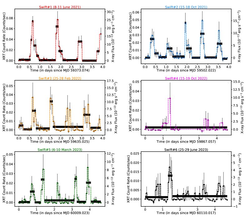
Figure 1: 0.3-1.2 keV X-ray light curves of eRO-QPE1. Each light curve is from a high-cadence monitoring program with Swift. The observation dates are indicated at the top of each panel. Both the X-ray count rate and the observed flux were measured in the 0.3-1.2 keV band. The decrease in strength of eruptions over time is evident. Note that the y-scale is different in each panel. The thick black horizontal lines are the optimal time bins derived from the Bayesian blocks algorithm of Scargle et al. 2013.

Broadly speaking, QPEs have the following observational properties. They all have soft/thermal spectra with best-fit blackbody temperatures of a few 10s to a few 100s of eV (Arcodia et al., 2021; Miniutti et al., 2019). There is no commonality in their burst profiles. For example, GSN 069, RX J1301.9+2747 and eRO-QPE2 have more or less symmetric bursts while eRO-QPE1 has a complex behavior where some eruptions show a fast-rise, slow decay behavior while others are more or less symmetric and can sometimes be broad (Arcodia et al., 2022). In general, their X-ray temperature is correlated with luminosity (Arcodia et al., 2021; Miniutti et al., 2019; Giustini et al., 2020). The recurrence time is not strictly periodic with GSN 069, RX J1301.9+2747, eRO-QPE1 and eRO-QPE2 showing variations on the order of $\approx$30% (Miniutti et al., 2023b; Giustini et al., 2020).

The underlying physical mechanism producing QPEs is currently unknown but an increased interest in this subject has led to several theoretical models being proposed in the last few years. These models can be put into two broad categories: ones that invoke inner accretion disk instabilities (Śniegowska et al., 2023; Kaur et al., 2023; Pan et al., 2022; Raj & Nixon, 2021) perhaps similar to those occurring in stellar-mass black hole X-ray binaries GRS 1915+105 (Neilsen et al., 2011) and IGR J17091-3624 (Altamirano et al., 2011), and those involving one or more orbiting stellar objects (Krolik & Linial, 2022; Linial & Sari, 2023; King, 2020; Metzger et al., 2021; Linial & Metzger, 2023; Suková et al., 2021; Franchini et al., 2023; Zhao et al., 2022; Xian et al., 2021). It has also been proposed that self-lensing binary supermassive black holes (SMBHs) can, in principle, produce quasi-periodic flares, but this scenario appears to be inconsistent with data from GSN 069 and RX J1301.9+2747 (Ingram et al., 2021). As evident in the extensive list of theoretical models referenced above, the models with an orbiting object around a massive black hole have increased the excitement in the field as QPEs could potentially represent extreme mass ratio inspirals (EMRIs) of a secondary orbiter gradually sinking down to the central SMBH. If that is the case, some studies have suggested that some QPE sources could be detectable by future space-based gravitational wave missions like LISA and Tianqin (Zhao et al., 2022). But Chen et al. (2021) have argued that the signals from the currently known QPE sources may be weak to be detectable by future gravitational wave detectors. Irrespective of the underlying mechanism, QPEs have opened up a unique new window into the inner accretion flows of massive black holes.

To pin down the mechanism driving QPEs, observations constraining their long-term evolution are necessary. Such information is available in the published literature only for GSN 069 (Miniutti et al., 2023b, a). Here we present results from a monitoring campaign over an extended temporal baseline of three years using Neil Gehrels Swift (Swift hereafter) and archival XMM-Newton observations of eRO-QPE1/2MASS 02314715-1020112 which exhibited QPEs separated by $\approx$0.8 d during the first monitoring dataset (Arcodia et al., 2021). We performed additional high-cadence observations on multiple epochs, and our main observational findings are discussed in section 2.

Epoch	MJDstart	MJDend	Count Rate	Counts	Average kT	Average	Peak	Quiescence
	(days)	(days)	(counts/sec)		(keV)	Flux	Flux	Flux
Swift#1	59373.074	59376.986	0.0244$\pm$0.0016	223	0.13$\pm$0.01	8.0$\pm$0.7	20.6$\pm$3.1	$<$0.3
Swift#2	59502.022	59505.948	0.0126$\pm$0.0012	124	0.13$\pm$0.01	3.9$\pm$0.4	11.5$\pm$2.2	$<$0.4
Swift#3	59635.025	59638.941	0.0099$\pm$0.0011	94	0.097$\pm$0.012	3.1$\pm$0.6	9.7$\pm$2.8	$<$0.3
Swift#4	59867.057	59871.634	0.0058$\pm$0.0016	15	0.097$\pm$0.012	1.7$\pm$0.6	6.5$\pm$3.9	$<$0.4
Swift#5	60009.023	60013.651	0.0096$\pm$0.0012	64	0.12$\pm$0.016	2.3$\pm$1.1	7.1$\pm$3.8	$<$0.2
Swift#6	60110.017	60114.723	0.0043$\pm$0.0008	33	0.12$\pm$0.016	1.1$\pm$0.4	3.2$\pm$1.7	$<$0.3

Table 1: Summary of eRO-QPE1’s Swift/XRT data and spectral modeling of its eruptions. Here 0.3-1.2 keV Swift/XRT spectra were fit with tbabs*ztbabs*zashift(diskbb) model using XSPEC (Arnaud, 1996). MJD_start and MJD_end represent the start and the end times (in units of MJD days) of the Swift monitoring campaign. Count Rate and Counts represent background-subtracted values in 0.3-1.2 keV. The column density at the host, ztbabs, was fixed at the best-fit XMM-Newton value of 0.069$\times$10²² cm^-2. Temperatures of Swift #1 and Swift #2, Swift #3 and Swift #4, and Swift #5 and Swift #6 were tied. All the errorbars represent 1-$\sigma$ uncertainties except for the 3$\sigma$ quiescence level upper limits. The Average Flux, Peak Flux and Quiescence Flux values correspond to 0.3-1.2 keV and have units of 10^-13 erg s ^-1 cm^-2. The total C-stat/degrees of freedom was 31.6/34.

2 Data and Observational Findings

Swift’s X-Ray Telescope (XRT; Burrows et al. 2005) performed six sets (Swift #1…6; Table 1) of high-cadence monitoring observations of eRO-QPE1. A detailed discussion of data reduction and spectral analyses is discussed in Appendix section A. Here we highlight the main observational findings.

Eruptions were detected in all these campaigns but with decreasing strength over time. This is evident even by eye in Fig. 1 where the brightness at peaks is gradually decreasing with time. The same is quantified in the top panel of Fig. 2 which shows that the peak and average fluxes of the eruptions have decreased by approximately a factor of 10 and 4, respectively, over three years. The quiescent level was detected in the first XMM-Newton observation but only upper limits were available during the Swift observations (Fig. 2 bottom panel).

Another key observational finding is that the recurrence time varies from one monitoring campaign to the next. Surprisingly, the three eruptions seen in the first Swift campaign (Swift #1) were separated by $\sim$1.1 days (left panel of Fig. 3), i.e., $\sim$40% longer than previously published recurrence time of 0.8 days (Arcodia et al., 2021). However, this recurrence time returned to a mean value of 0.8 d roughly six months later in Oct 2021 (Swift #2; right panel of Fig. 3). This is also quantified in the Lomb Scargle Periodograms shown in Fig. 4. Over the course of all the six monitoring campaigns, the recurrence time varied between 0.6 and 1.2 days (see section A.1 and Fig. 4).

While several eruptions reported here are consistent with a fast-rise and smooth decay profile reported in Arcodia et al. 2021, there are numerous examples of more complex profile shapes. For example, the second eruption in Swift #2 has a extended decay. The 4^th and the 5^th eruptions (around days 2.3 and 3.3) in Swift #3 have a dip near their peaks. The eruption around day 1.5 in Swift #6 and the last two eruptions in Swift #2 appear symmetric in shape. In summary, contrary to previous reports, we find that the eruption profiles have different shapes. This is an important aspect to stress as Arcodia et al. (2021) used the fast-rise and slow decay profile as an argument against a certain type of radiation pressure instability.

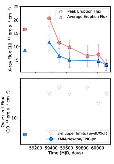
Figure 2: Long-term Evolution of the average peak luminosity of the eruptions (top) and the quiescent level (bottom). The fluxes are observed values in the 0.3-1.2 keV band. The errorbars represent 1$\sigma$ uncertainties. They include both measurement and model fitting uncertainties (see section A.1). Swift/XRT data were not sensitive enough to detect the quiescent level but 3$\sigma$ upper limits are shown. XMM-Newton’s observed 0.3-1.2 keV quiescent flux was derived from combining data from obsIDs 0861910201 and 0861910301 (blue point in the bottom panel).

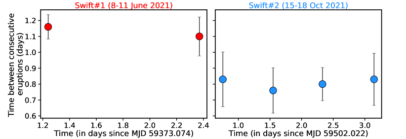
Figure 3: Evolution of time between consecutive eruptions with time for Swift #1&2 datasets. The peaks of eruptions were determined in a model-independent manner using the Bayesian blocks algorithm of Scargle et al. 2013. These values are consistent with the Lomb Scargle peaks shown in Fig. 4.

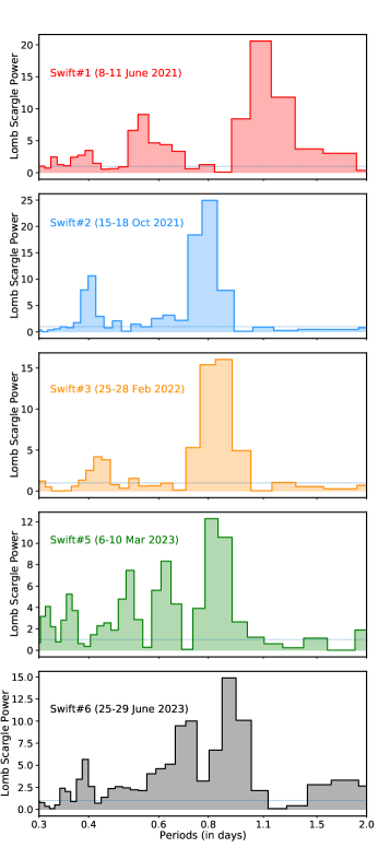
Figure 4: Lomb Scargle Periodograms of the light curves shown in Fig. 1. Here were zoom in on the 0.3-2.0 days timescale. The highest peaks (corresponding full width at half maximum) for Swift #1, Swift #2, Swift #3, Swift #5, and Swift #6 are 1.09${}^{+0.23}_{-0.08}$ d, 0.81${}^{+0.03}_{-0.10}$ d, 0.83${}^{+0.09}_{-0.07}$ d, 0.82${}^{+0.10}_{-0.04}$ d, and 0.91${}^{+0.12}_{-0.25}$ d, respectively. We do not show the LSP from Swift #4 as it was affected by a large data gap. The blue/dashed horizontal line at a power value of 1 represents the LSP’s nominal white noise level. While the main purpose of these plots is to show the evolution of the main LSP peak and not to delve into the details of the LSP, it is interesting that a harmonic is also present in all cases at roughly 1/2 the period of the main peak.

3 Implications for various theoretical models

We now discuss the observations presented above within the context of various models proposed for QPEs.

3.1 QPEs models with orbiting objects

3.1.1 Repeating partial Tidal Disruption Event (TDE)

First, we explore three flavors of repeating partial TDE (rpTDE) scenarios: 1) eRO-QPE1’s central black hole is repeatedly disrupting a star on a timescale of several years and the QPEs are produced as a result of inner disk-related physics, 2) QPEs are a direct result of a white dwarf that is in a $\sim$1 day orbit around an SMBH, and 3) rpTDE of a main sequence star by an SMBH.

Miniutti et al. (2023b) noted that GSN 069’s long-term behavior appears to be consistent with the tidal disruption of a star, and the QPEs only appeared once the flux fell below a critical value. It may therefore be the case that the QPE phenomenon is intricately tied to, and in fact requires, a prior TDE, with the production mechanism related to the ensuing disk physics (and any potential instabilities associated therewith) or a change in the morphology of the returning debris stream (Coughlin & Nixon, 2020; Guolo et al., 2023). Unfortunately, the quiescent X-ray flux from eRO-QPE1 is below the Swift/XRT detectability threshold (see Figure 2), and we are not presently able to test this hypothesis. However, future XMM-Newton monitoring observations can address the nature of the long-term evolution of quiescence emission (see section 4.2).

A second scenario has been suggested in which the X-ray eruptions are produced due to accretion following the repeated partial tidal stripping of a white dwarf by the black hole in the nucleus of the galaxy (King 2020; see also Zalamea et al. 2010 in the context of Extreme Mass Ratio Inspirals/EMRIs). If the energy generated due to accretion is $E_{\rm acc}=\eta{M}c^{2}$ with $\eta=0.1$, then using a luminosity distance of 233 Mpc alongside the mean observed eruption flux of 3.4$\times$10^-13 erg s^-1 cm^-2 (see Figure 2) implies an X-ray (0.3–1 keV) energy release per outburst of $E\simeq 7\times 10^{46}$ erg (average flux$\times$4$\times\pi$(luminosity distance)${}^{2}\times(1+z=0.0505)\times$(average eruption duration of 8 hours from Arcodia et al. 2021)), and hence an accreted mass of $M_{\rm acc}=E_{\rm acc}/(0.1c^{2})\simeq 4\times 10^{-7}M_{\odot}$. For a white dwarf with mass $\sim{\rm few}\times 0.1M_{\odot}$, this amounts to a very small fraction of the total mass of the star, implying that the pericenter distance of the white dwarf is extremely fine-tuned to coincide with its partial tidal disruption radius (i.e., where material is just barely able to be removed from the surface of the star). How the star achieved precisely this distance is not clear, as neither gravitational-wave emission nor tidal interactions can dramatically change the pericenter distance. However, because the amount of mass stripped from the star is a very sensitive function of distance (see Guillochon & Ramirez-Ruiz 2013), we might expect variation in the mass accreted – and hence the luminosity (according to this model) – even for small changes to the pericenter due to, e.g., the exchange of angular momentum between the star and the orbit. These secular changes are consistent with eRO-QPE1’s trend in Figure 2.

Additionally, eRO-QPE1’s black hole is estimated to be $\sim 10^{6}M_{\odot}$ (Wevers et al., 2023), which implies that the pericenter distance of the star must be highly relativistic – at most on the order of a few gravitational radii. Adopting a white dwarf mass of $0.6M_{\odot}$ and a corresponding radius of $R_{\star}=0.011R_{\odot}$ (Nauenberg, 1972) yields a tidal disruption radius of $0.6GM_{\rm BH}/c^{2}$, i.e., the partial tidal disruption radius is about twice that value (Guillochon & Ramirez-Ruiz, 2013) at $\sim 1.2GM/c^{2}$. If we set the pericenter distance of the star to $1.2GM/c^{2}$ (which requires a rapidly spinning black hole and a prograde orbit for the star to not be directly captured), and the semi-major axis is determined from the recurrence period of $T=1$ day to be $a=(T\sqrt{GM}/(2\pi))^{2/3}\simeq 200GM/c^{2}$ for $M=10^{6}M_{\odot}$, then this corresponds to an eccentricity of $e\simeq 0.994$. For these parameters, the gravitational-wave inspiral time can be estimated from Equations 5.6 and 5.7 from Peters (1964), and is $\sim 3.2$ years, i.e., the source would have declined substantially in recurrence time during the three years over which it has been observed. This is in obvious disagreement with the behavior exhibited by eRO-QPE1, which has a recurrence time that is relatively stable (see Figure 4).

More generally, we can calculate the time-dependent evolution of the orbital parameters (i.e., the semimajor axis and the eccentricity) by integrating Eqs. (5.6)–(5.7) of Peters (1964) for different black hole and stellar masses. Figure 5 shows the orbital period of the white dwarf as a function of time in years for four different black hole masses; the left panel uses a white dwarf mass of $M_{\star}=0.6M_{\odot}$ (also used by King 2020 and where the mass distribution of white dwarfs peaks), while the right panel adopts $M_{\star}=0.4M_{\odot}$. Here we assumed an initial orbital period of 1 day, a pericenter distance equal to twice the tidal radius $r_{\rm t}=R_{\star}\left(M_{\bullet}/M_{\star}\right)^{1/3}$, and the mass-radius relationship $R_{\star}=0.011\left(M_{\star}/(0.6M_{\odot}\right)^{-1/3}R_{\odot}$, which is valid for a non-relativistic (i.e., for a lower-mass white dwarf) fully degenerate gas. We use the leading-order Newtonian estimates for the tides, gravitational radiation, and orbital dynamics. Since the orbit is highly relativistic, there will be substantial corrections beyond the lowest-order solution given in Peters (1964) (see, e.g., Blanchet 2014; Tucker & Will 2021). These higher-order terms generally lead to accelerated decay of the eccentricity and period shortening, especially for the case of heavier central SMBH, even though the qualitative picture stays the same. Thus, the results shown in Figure 5 should be considered upper limits to the orbital period as a function of time, i.e., higher-order terms will only result in an acceleration in the decay rate of the period.

This figure shows that for a white dwarf mass of $M_{\star}=0.6M_{\odot}$, the orbital period decays substantially – by at least a factor of 2 – until the black hole mass is well below the value inferred from the $M-\sigma$ relation and into the intermediate-mass black hole regime. For $M_{\star}=0.4M_{\odot}$ the period decays by at least $\sim 15\%$ for $M_{\bullet}=10^{5}M_{\odot}$, and only for $M_{\bullet}=10^{4}M_{\odot}$ and $M_{\bullet}=10^{3}M_{\odot}$, i.e., intermediate-mass black holes, is the period change sufficiently small that it would remain undetected over the three-year observational period of eRO-QPE1. This figure shows that, if eRO-QPE1’s eruptions are produced from the repeated tidal stripping of a white dwarf, the black hole mass must be substantially smaller than the one inferred from $M-\sigma$, or the white dwarf mass must be very small (making the star rare).

We also note that, for partial disruptions in which $\gtrsim 10\%$ of the mass of the star is removed, which corresponds to pericenter distances smaller than $\sim r_{\rm t}/(0.65)$ for a 5/3-polytropic star (Guillochon & Ramirez-Ruiz, 2013; Mainetti et al., 2017; Miles et al., 2020), higher-order moments (i.e., beyond the quadrupole) of the gravitational field of the black hole induce a positive-energy kick to the surviving star (and this has been verified across a wide range of black hole masses and stellar/planetary types; e.g., Faber et al. 2005; Manukian et al. 2013; Gafton et al. 2015; Kremer et al. 2022). This effect could conceivably stabilize the orbital decay that is induced by the gravitational-wave emission. However, for the extremely small amount of mass lost by the star necessary to power QPEs, the stellar pericenter distance is such that the tidal excitation of modes in the star removes energy from the orbit (i.e., the star is in the classic tidal dissipation regime; Fabian et al. 1975; Press & Teukolsky 1977). Specifically, it was recently shown by Cufari et al. (2023) that, for a pericenter distance of $r_{\rm t}/(0.55)$ – very close to the distance from the black hole at which almost no mass is lost from the star – the change in the specific energy of the orbit is $\Delta\epsilon\simeq-0.025GM_{\star}/R_{\star}$ and is roughly the maximum amount by which tides reduce the energy of the orbit (i.e., larger pericenter distances yield less tidal excitation, but smaller pericenter distances lead to a positive-energy kick; see Figure 1 in Cufari et al. 2023). In this case, the fractional change in the energy of the orbit is $\Delta\epsilon/\epsilon=0.025M_{\star}a/(M_{\bullet}R_{\star})\sim 0.1\%$ for $M_{\star}=0.6M_{\odot}$, $R_{\star}=0.011R_{\odot}$, $M_{\bullet}=10^{6}M_{\odot}$, and $a=200GM_{\bullet}/c^{2}$, which is comparable in magnitude to the per-orbit change in energy induced by gravitational-wave emission. Thus, in this case we would only expect tides to accelerate the inspiral.

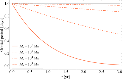
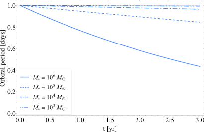
Figure 5: The Keplerian orbital period of a white dwarf orbiting a massive black hole, with black hole mass indicated in the legend, as a function of time in years, where the left (right) panel adopts a white dwarf mass of $M_{\star}=0.6M_{\odot}$ ($0.4M_{\odot}$). The pericenter distance is equal to twice the canonical tidal radius, while the orbital period is initially equal to the recurrence time of 1 day. Over the course of the observations of eRO-QPE1, being roughly 3 years, there would be a substantial and noticeable decline in the recurrence time of the flares owing to gravitational-wave emission, unless the black hole mass is significantly below the value inferred from the $M-\sigma$ relation (being $\sim 10^{6}M_{\odot}$), or the white dwarf mass is significantly smaller than the mean value of $\sim 0.6M_{\odot}$.

In the third scenario of repeated partial disruption of a main sequence star, it is also difficult to reconcile the observed timescales and energetics of QPEs. This model has been invoked to explain the repeating nuclear transients ASASSN-14ko (Payne et al., 2021), AT2018fyk (Wevers et al., 2023), eRASSt-J0456 (Liu et al., 2023), and Swift J0230 (Evans et al., 2023; Guolo et al., 2023). Specifically, we would expect the return time of the tidally stripped debris to be comparable to the dynamical time at the surface of the star, multiplied by the square root of the mass ratio of the black hole to the star (Lacy et al., 1982; Rees, 1988). For a white dwarf, this timescale is of the order of a ksec – in rough agreement with the flare duration of QPEs – while for main sequence stars it is $\sim few\times 10$ days (see, e.g., the simulations in Guillochon & Ramirez-Ruiz 2013; Golightly et al. 2019; Law-Smith et al. 2020; Nixon et al. 2021), which is orders of magnitude longer than the flare duration in QPEs, in general. Similar to the white dwarf model, the extremely small amount of mass accreted per burst is also problematic, and requires fine tuning to achieve a pericenter distance that is very closely aligned with the partial disruption radius of a star.

3.1.2 QPEs from interactions of an orbiting perturber with the accretion disk

Suková et al. (2021) proposed that QPEs could be produced from repeated interaction of an object with the accretion disk of an SMBH (see also Xian et al., 2021; Franchini et al., 2023; Linial & Metzger, 2023). In their model, at each interaction, the perturbation causes: 1) the modulation of the accretion rate onto the black hole depending the ratio of the influence radius of the object to its distance, and 2) ejection of matter clumps towards the magnetic poles, which can drive a quasiperiodic ultrafast outflow. Assuming that the perturber period is equal to twice the eruption period (two eruptions per orbit, i.e. $P_{\rm orb}\sim 2\times 0.9$ days), the semi-major axis is given by $a\sim 399.3(P_{\rm orb}/1.8\,\text{days})^{2/3}(M_{\bullet}/10^{5.8}\,M_{\odot})^{-2/3}R_{\rm g}$, where $R_{\rm g}=GM_{\bullet}/c^{2}$ is a gravitational radius of the SMBH. Hence, it would vary between $\sim 1003\,R_{\rm g}$ for $M_{\bullet}=10^{5.2}\,M_{\odot}$ and $\sim 159\,R_{\rm g}$ for $M_{\bullet}=10^{6.4}\,M_{\odot}$.

The varying recurrence time in Fig. 4 and 3 can be addressed well by the Schwarzschild precession of the orbit, which can modulate the recurrence timescale, especially for mildly eccentric orbits. Using the formula for the periapse (Schwarzschild) precession, the timescale for the apsidal rotation by $90^{\circ}$ can be expressed as follows,

$$\tau_{\frac{\pi}{2}}\sim 80.3\left(\frac{P_{\rm orb}}{2.2\,\text{days}}\right)^{\frac{5}{3}}\left(\frac{M_{\bullet}}{10^{5.8}\,M_{\odot}}\right)^{-\frac{2}{3}}\left(\frac{1-e^{2}}{0.96}\right)\,\text{days}\,,$$ (1)

where $e$ is the orbital eccentricity, which is set to $e=0.2$. This implies that the orbital orientation with respect to the accretion disk changes on the timescale of 100 days due to the periapse precession and this can thus partially address the changing eruption recurrence. For instance, initially, for a highly inclined perturbing body, the orbital orientation when the perturber intersects the disk at the apoapse and the periapse has the eruption periodicity of $\sim 1.1$ days or half of the orbital period. In $\tau_{\frac{\pi}{2}}\sim 80$ days, both intersections are close to the periapse, specifically the eruption recurrence timescale is $0.82$ days for $e=0.2$. This is comparable to the change in the recurrence timescale between Swift 1 and 2 datasets, see Figure 3. Since the Swift monitoring was separated by a few months and lasted always only a few days, for each monitoring session we effectively capture the system in a specific orbit-disk orientation and hence the recurrence timescale would vary accordingly.

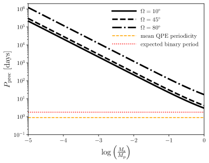
Figure 6: Accretion disk’s precession period due to the torques by the secondary (expressed in days) as a function of the logarithm of the component mass ratio ($\log{(M_{\rm s}/M_{\rm p})}$). We depict three cases corresponding to the low inclination of the secondary with respect to the accretion disk ($\Omega=10$ degrees, solid line), intermediate inclination ($\Omega=45$ degrees, dashed line), and high inclination of $\Omega=80$ degrees (dot-dashed line). The mean QPE periodicity and the expected binary period are represented by dashed orange and red dotted lines, respectively.

Further variations can be caused by the disk precession (see also Franchini et al., 2023), which can take place on various timescales depending on the outer radius of the misaligned disk and the black hole spin when the disk precession is rigid-like and driven by the Lense-Thirring effect. The Lense-Thirring precession also leads to the rotation of the line of nodes for the orbiting body that also affects the timing between the eruptions, especially for perturbers close to the rotating SMBH.

The disk precession can also be driven by the torques from the misaligned object and the precession period in that case is longer than the orbital period. The disk precession due to the torques from the orbiting secondary has a timescale of a few hundred days to days for massive perturbers of at least $\sim 10^{4}\,M_{\odot}$ for the total mass (primary$+$secondary) of $10^{6}\,M_{\odot}$. More specifically, for the secondary to primary mass ratio of $M_{\rm s}/M_{\rm p}=10^{-2}$, the precession period is $214$ days and for $M_{\rm s}/M_{\rm p}=10^{-1}$ the precession period is 22 days, assuming the inclination of $\Omega=10$ degrees between the secondary and the accretion disk around the primary. In Fig. 6, we plot the expected precession period as a function of the mass ratio adopting the model of Papaloizou & Terquem (1995), Larwood (1997), and Britzen et al. (2018). We consider three inclinations (10, 45, and 80 degrees), a polytropic index for the non-relativistic gas ($n=3/2$), the semi-major axis of $\sim 0.014$ milliparsecs (corresponding to the orbital period of $\sim 1.8$ days), and the outer radius of the precessing disk corresponding approximately to the semi-major axis of the binary. We see that the precession period of a few days is only possible for nearly equal-mass components.

Another reason for changes in periodicity could be the time lag between the perturber-disk interaction and the time when the perturbation reaches the SMBH. The thermal front propagation is given by the sound-crossing timescale as $t_{\rm front}\approx R/(\alpha c_{\rm s})\sim(H/R)^{-1}t_{\rm th}$, where the thermal timescale can be estimated as $t_{\rm th}\sim\alpha^{-1}[R^{3}/(GM_{\bullet})]^{1/2}\sim 0.36(\alpha/0.1)^{-1}(R/100R_{\rm g})^{3/2}(M_{\bullet}/10^{5.8})\,\text{days}$. For the scale-height to radius ratio of $H/R\sim 0.1$, the front propagation timescale is $t_{\rm front}\sim 3.6[(H/R)/0.1]^{-1}(\alpha/0.1)^{-1}(R/100R_{\rm g})^{3/2}(M_{\bullet}/10^{5.8})\,\text{days}$. Therefore the eruption recurrence timescale can be modulated by the propagation timescale that is further affected by the disk thickness, and hence the current accretion state.

While in the perturber-disk interaction model presented by Suková et al. (2021) the eruptions are produced by quasi-periodic enhancements in the accretion rate, in the analogous models presented by Linial & Metzger (2023) and Franchini et al. (2023), the X-ray emission flare is produced in shocked, optically thick expanding clouds of disk material ejected above and below the disk (e.g., see discussion in Linial & Metzger, 2023). In principle, both emission mechanisms – accretion-based and shock-based – could be at work. The decreasing amplitude of eruptions in Fig. 2 is consistent with models of Suková et al. (2021); Franchini et al. (2023); Linial & Metzger (2023). It can be attributed to diminishing inclination between the perturber’s orbit and the accretion disk, which decreases the relative velocity of the perturber with respect to the disk material, and hence the energy generated in density waves and shocks. Such an alignment process can take place due to the ongoing Bardeen-Petterson effect if the accretion disk is initially misaligned with respect to the equatorial plane. Alternatively, it could also be the result of the disk surface density becoming lower due to an ongoing decrease in the accretion rate. This follows from the eruption luminosity being proportional to the disk surface density, $L_{\rm QPE}\propto\Sigma$ (Linial & Metzger, 2023; Tagawa & Haiman, 2023), and for the standard disk there is a power-law dependency of the surface density on the accretion rate, $\Sigma\propto\dot{m}^{7/10}$ (Frank et al., 2002). The accretion rate can be decreasing over the course of several months to years following a TDE (see e.g. Linial & Metzger, 2023, and further discussion) with a power-law time-dependency, in particular $\dot{m}\propto t^{-5/3}$ for the canonical TDE, and hence $L_{\rm QPE}\propto t^{-7/6}$. One of the key differences between models proposed by Suková et al. (2021) and those by Franchini et al. (2023) and Linial & Metzger (2023) is that the former predicts the presence of repeated outflows. However, the search for such outflows is beyond the scope of this letter.

As discussed in Linial & Metzger (2023), the emission properties of QPEs may secularly evolve due to changes in the accretion flow, and specifically the disk’s scale-height and accretion rate, as well as changes to the secondary object’s physical radius. If the secondary is a star, its outer layers are repeatedly ablated by shocks at every disk passage, consequently changing the star’s cross section and its interaction with the disk. Linial & Metzger (2023) further proposed that the origin of the accretion disk is bound debris of a previously tidally disrupted star around the same SMBH. The long term evolution of the TDE disk naturally results in evolution timescales of order years-decade (e.g., their equations 34-35), in agreement with the trends observed in the data. Another outcome of star-disk interaction is the orbital decay induced by hydrodynamical drag at disk passages. However, this should lead to a rather slow, gradual decrease in the recurrence timescale unlike a rather abrupt change of the recurrence timescale from 1.1 days in June, 2021 to 0.8 days in October, 2021, i.e. over the course of four months. The stellar orbit can only be abruptly changed by a massive mass loss from the system, for example, when a distorted stellar body would split like in a Hills mechanism.

The star-disk interaction model was also presented by Tagawa & Haiman (2023), where the QPE luminosity is dominated by the breakout emission of the bow-shock of the star as it emerges from the AGN disk. They argue that for eRO-QPE1 both the breakout emission as well as the cooling emission of the expanding shocked bubble could contribute. This could partially address multiple peaks in Lomb-Scargle periodograms since the breakout emission should contribute once per orbit (when we see the emerging bow shock as the star ascends above the accretion disk), while we detect the cooling emission twice due to the expansion of the shocked gas both above and below the accretion disk. On the other hand, their model requires massive stars ($\sim 10\,M_{\odot}$) on retrograde, low-inclination orbits, which appears to be rather restrictive.

Finally, it is important to note that the shape of the eccentric orbits with a smaller pericenter distance near a fast-spinning black hole can be very different from Keplerian-like ellipses (e.g. Chandrasekhar, 1998, chapt. 7). In fact, the disk-crossing radius can fluctuate in a rather wide range, thus giving a possibility to explain changes of the outburst properties (Karas & Vokrouhlický, 1994; Xian et al., 2021; King, 2023).

3.1.3 QPE from Roche-lobe overflow from a star orbiting an SMBH

Roche-lobe overflow from an orbiting star was suggested to explain several QPE properties, such as their peak luminosities, temperatures, and the flare durations (Krolik & Linial, 2022; Linial & Sari, 2023) . In that case a small fraction of the stellar envelope is tidally stripped close to the pericenter of the stellar orbit. Therefore the eruption recurrence timescale is given by the orbital period, which sets the semi-major axis to $a\sim 251.6(P_{\rm orb}/0.9\,\text{days})^{2/3}(M_{\bullet}/10^{5.8}\,M_{\odot})^{-2/3}R_{\rm g}$. The X-ray eruptions could be produced via the oblique stream-stream shocks close to the innermost stable circular orbit, which can address the soft X-ray thermal emission corresponding to $\sim 110$ eV. The stellar orbit is expected to be only mildly eccentric ($e\lesssim 0.5$). In that case, for the soft X-ray eruptions to be produced close to the innermost stable circular orbit, the detached stellar stream needs to lose its specific angular momentum that is initially comparable to the orbital angular momentum of the star at the pericenter crossing. This can be achieved by several processes, such as induced magnetic stresses (Krolik & Linial, 2022) and/or magnetohydrodynamic drag due to ambient hot plasma (Zajaček et al., 2014), especially when the stellar orbit is more compact on the scale of a few $10\,r_{\rm g}$, i.e. the model can thus work better for eRO-QPE1 when the SMBH is heavier with $\sim 10^{6.4}\,M_{\odot}$. Assuming that most of the energy is dissipated at $R_{\rm dis}\sim 10\,R_{\rm g}$ due to oblique stream-streamshocks driven by apsidal precession, the mean stellar mass loss per eruption can be estimated as $\Delta M\sim 7\times 10^{-7}\,(L_{\rm erupt}/2.2\times 10^{42}\,{\rm erg\,s^{-1}})(\tau_{\rm erupt}/8\,\text{h})(R_{\rm dis}/10\,R_{\rm g})\,M_{\odot}$, where $L_{\rm erupt}$ is the mean eruption luminosity and $\tau_{\rm erupt}$ is the mean eruption duration. The system SMBH–star is relatively long-lived since the stellar body is depleted in $\tau_{\star}=(M_{\star}/\Delta M)P_{\rm orb}\sim 3500$ years. The merger timescale for the orbital period of $P_{\rm orb}\sim 0.9$ days and a nearly circular orbit is $\tau_{\rm merge}\sim 4.85(P_{\rm orb}/0.9\,\text{days})^{8/3}(M_{\bullet}/10^{5.8}\,M_{\odot})^{-2/3}(M_{\star}/1\,M_{\odot})^{-1}$ Myr, hence about three orders of magnitude longer than $\tau_{\star}$. The irregularity of the eruption recurrence can be caused by the intense X-ray irradiation of the upper stellar atmosphere. This stems from the comparison of the X-ray and stellar flux densities at the periapse (Krolik & Linial, 2022),

$$F_{\rm X}/F_{\star} \sim 6\times 10^{3}(1-e)^{-2}(L_{\rm erupt}/2.2\times 10^{42}\,{\rm erg\,s^{-1}})\times\,$$

$$(P_{\rm orb}/0.9\,\text{days})^{-4/3}(M_{\bullet}/10^{5.8}\,M_{\odot})^{-2/3}(T_{\star}/T_{\odot})^{4}\,.$$ (2)

The maximum unbound mass per orbit escaping the star due to the excess heating by the X-ray eruption can be estimated as follows,

$$\Delta M_{\rm unbound} \sim 3\times 10^{-8}(1-e)^{-2}(L_{\rm erupt}/2.2\times 10^{42}\,{\rm erg\,s^{-1}})\times\,$$

$$(D_{\rm erupt}/0.3)(P_{\rm orb}/0.9\,\text{days})^{-1/3}\times\,$$

$$(M_{\bullet}/10^{5.8}\,M_{\odot})^{-2/3}(M_{\star}/1\,M_{\odot})^{1.64}\,M_{\odot}\,,$$ (3)

where $D_{\rm erupt}$ is the duty cycle of eruptions. For mildly eccentric orbits ($e\sim 0.5$), $\Delta M_{\rm unbound}$ is comparable to $\Delta M$, and hence the modulation of mass transfer and QPE luminosity via the excess heating is a plausible mechanism. The stellar mass transfer may thus be initially enhanced and unstable due to the induced turbulence in the upper atmosphere. In addition, the progressive tidal truncation of the star may lead to its shrinking when the atmosphere layer is depleted via the Roche-lobe overflow. The short periodicity of $\sim 0.9$ days is consistent with a Solar-like star whose radius is comparable to the Roche-lobe radius at its pericenter. The required stellar radius has an approximately Solar value. Using the relation for the limiting stellar radius for the tidal stripping, $R_{\star}\sim G^{1/3}/(4\pi^{2})^{1/3}(1-e)P_{\rm orb}^{2/3}M_{\star}^{1/3}$, we obtain the numerical estimate of $R_{\star}/R_{\odot}\sim 3.92(1-e)(P_{\rm orb}/0.9\,{\rm days})^{2/3}(M_{\star}/1\,M_{\odot})^{1/3}$. Hence, if the stellar radius slightly shrinks below this value, the flares may be weakened or fall below the detection limit. The stripping of the envelope can also be connected with the inspiral of the star, and thus shortening of the QPE period (Bogdanović et al., 2014). However, the precise timing of these processes requires 3D hydrodynamical models involving a realistic stellar model that is subject to tidal forces and radiation heating due to the X-ray flare close to the pericenter.

A modification of the Roche-lobe overflow model was presented by Lu & Quataert (2023), where the Roche-lobe overflowing star feeds a compact accretion disk. As in Krolik & Linial (2022), the QPE emission is due to circularization shocks, hence not accretion dominated. The steady-state accretion disk should provide a quiescent accretion with the Eddington ratio of $\sim 0.08$ (their Eq. 12) for $M_{\bullet}=10^{6}\,M_{\odot}$, which is above the inferred upper limit on the quiescent X-ray luminosity of eRO-QPE1.

3.2 QPE models related to accretion flow instabilities

3.2.1 QPEs from radiation pressure instability

Accretion disk instabilities were invoked already in early studies (Lightman & Eardley, 1974) and revealed that the innermost regions of viscous disks cannot be stable when reaching a significant fraction of Eddington luminosity. In the unstable mode, the radiation pressure becomes so strong that the local cooling exceeds the heating. When the local temperature increases, the excess of accretion rate leads to the disk depletion and density drops. The disk can rebuild on short timescales and enter a cyclic oscillatory mode, if the advective process is regulating the thermal imbalance. Numerical simulations of such oscillations presented in Janiuk et al. (2002) and the theoretical lightcurves well matched the observations of Galactic microquasars, GRS 1915+105, and then IGR J17091 (see Janiuk et al. 2015). The extension of the unstable zone, and hence amplitudes and timescales of the observable luminosity flares, depend on the mass inflow rate, and also on the mass of the central black hole. Application of the same global disk instability model to a wide range of black hole masses, from stellar mass to intermediate and SMBH, is quite straightforward. However, in order to produce realistic patterns, certain modifications of disk physics have to be assumed. For instance, Grzedzielski et al. (2017) considered alternative forms of the viscous stress tensor, and found out that oscillation periods on the order of 1 day are possible for an IMBH of a 4$\times$10⁴ M_⊙. The ratio of flare width to the recurrence time between flares is another measurable quantity, that may help to verify this model and its parameters. Alternatively, Śniegowska et al. (2023) discussed explicitly the role of magnetic fields in regulating the oscillation pattern and partial stabilisation of the disk. For the case of $10^{5}M_{\odot}$ black hole, the intra-day oscillation timescales, characteristic of the QPE phenomenon, are possible with a strong magnetic field. For the accretion rate of $\dot{m}$ = 0.5, and magnetic field of coefficient $b=0.22$ decreased the outburst timescale to $\sim$days. In this case, the pattern is irregular, and few-day flares are accompanied by sequences of one-day outbursts. In addition, changing the viscosity parameter to $\alpha=0.1$ shortened the outburst timescale down to $16$ hours. We note that the shape of the outbursts obtained from radiation pressure instabilities is asymmetric and the dimming phase takes 10% of the duration of the full flare, which appears to be in contradiction with fast rise-slow decay or symmetric profiles of most of the flares of eRO-QPE1. In addition, considering the upper limit on the quiescent-level flux of eRO-QPE1, $F_{\rm q}\lesssim 4\times 10^{-14}\,{\rm erg\,s^{-1}\,cm^{2}}$, the Eddington ratio can be constrained to be $\dot{m}\lesssim(4\pi D_{\rm L}^{2}F_{\rm q})\kappa_{\rm bol}/L_{\rm Edd}\sim 0.03$ for $M_{\bullet}=10^{5.8}\,M_{\odot}$ and the bolometric correction of $\kappa_{\rm bol}\sim 10$ (Richards et al., 2006; Netzer, 2019). For the XMM-Newton’s quiescent flux of $F_{\rm q}^{\rm XMM}\sim 5\times 10^{-15}\,{\rm erg\,s^{-1}\,cm^{-2}}$, we obtain $\dot{m}\sim 0.004$. Hence, the relative accretion rate is at least one order of magnitude lower than the limiting accretion rate of $\dot{m}_{\rm RPI}\gtrsim 0.16\alpha_{0.1}^{41/29}m_{5.8}^{-1/29}$ that is required for the radiation-pressure instability to effectively operate (Sniegowska et al., 2020) within the radiation-pressure dominated standard accretion disk.

3.2.2 QPEs from shock front oscillations

Another possible source of QPEs is oscillations of the shock front in low angular momentum flows. The source of the low angular momentum material accreting onto the SMBH can be strong stellar winds from massive stars orbiting the central black hole on larger distances ($\sim$ parsec scale) as was estimated for Sgr A* by Mościbrodzka et al. (2006). If the accreting material on the central SMBH has sub-Keplerian angular momentum distribution, for a certain range of the parameter space (energy and angular momentum of the incoming matter) the possibility of multiple critical points existence appears (Paczynski & Bisnovatyi-Kogan, 1981; Muchotrzeb & Paczynski, 1982; Abramowicz & Kato, 1989). In such a case, a shock front connected with a sudden drop of the inward velocity from supersonic to subsonic regime and simultaneous increase of the flow density may emerge. The accretion solution then passes through both the outer and the inner sonic points. The relation of quasi-spherical slowly rotating accretion flows to variability of X-ray sources has been reported already by Jufu & Abramowicz (1988) and the parameter space corresponding to the shock emergence in different geometrical setup was described by Abramowicz & Chakrabarti (1990).

More recently, numerical simulations have shown, that for a subset of parameters, the shock front location is unstable and oscillations of the shock bubble develop (Suková & Janiuk, 2015), which is accompanied by quasi-periodic flares in the accretion rate. Suková et al. (2017) provided extended study of the dependence of the oscillations on angular momentum and energy by means of 1D/2D and 3D GRMHD simulations, while Palit et al. (2019) focused on the effect of adiabatic index on the resulting flow.

Considering the mass of the SMBH in the range $M\in(10^{5.2},10^{6.4})M_{\odot}$, the recurrence time of 0.9 days or $(10^{5}-6\times 10^{3})\,GM/c^{3}$ in geometrized units corresponds to the frequency $f\in(1\times 10^{-5},2\times 10^{-4})\,c^{3}/(GM)$. Such values were reported by Suková et al. (2017, see Table 3 and Fig. 18) for shock fronts oscillating at the distance of several tens of gravitational radii from the center.

The model can accommodate the variations in the period taking into account that the oscillations shown by Suková et al. (2017) are quasi-periodic in nature even when the parameters of the incoming gas (energy and angular momentum) are kept strictly constant. Moreover, the mean position of the shock front and the frequency of the oscillations depend quite strongly on those parameters, hence their relatively small change can lead to a change in the recurrence period or even to the disappearance/reappearance of the shock front, which is reflected in the accretion rate behaviour. The gradual decrease of the peak flux may be attributed to the slow density decline of the incoming gas.

The coherent oscillations of the shock front are expected to appear in a situation where the incoming gas has relatively stable properties falling inside the multicritical parameter space, which may be a short-lived situation depending on the properties of the gas on the larger scale.

3.2.3 QPEs from disk tearing instability

The disk tearing instability can occur in disks that are sufficiently misaligned to a spinning black hole such that a large warp amplitude can develop in the disk (Nixon et al., 2012; Doǧan et al., 2018; Raj et al., 2021). When only a modest warp amplitude is reached, the warp propagates through the disk either via waves if the disk is hot and low viscosity or diffusion if the disk is cool and high viscosity (Papaloizou & Pringle, 1983). However, for disks that achieve a large warp amplitude it has been shown that they can become unstable, leading to the disk separating into diskrete rings (Doǧan et al., 2018, see also Ogilvie 2000). In either the wavelike or diffusive case of warp propagation it is possible for the disk to tear into discrete rings (Drewes & Nixon, 2021). In disks that are strongly unstable, the disk emission can exhibit complex variability as the unstable region can be far from the black hole; this means that a combination of shocks, subsequent accretion and geometric effects are responsible for determining the emergent lightcurve. These processes are discussed in detail in Nixon & Salvesen (2014) and Raj & Nixon (2021).

However, for disks that are only weakly unstable, the instability is confined to the very inner regions of the disk. Raj & Nixon (2021) provide an example simulation of such a disk, where the innermost annulus of the disk is repeatedly torn off and accreted in a brief flare-like event. In their Fig. 3 they provide the accretion rate on to the central black hole with time, which shows regularly spaced peaks. They suggest that X-rays may be produced when the ring of gas that is torn from the disk precesses and shocks against its neighboring ring before falling into the black hole. For a black hole of mass $4\times 10^{6}\,M_{\odot}$ the spacing between these peaks is approximately a day, and thus could be consistent with the eruptions in eRO-QPE1. The shape of most of the eruptions observed in eRO-QPE1 (being fast rise and slower decay) are reversed compared to those seen in Fig. 3 of Raj & Nixon (2021); while this does not appear consistent, it may be that a more detailed model of the emission from the disk could account for this shape. For example, the shocks may cool slower than assumed in the simulation or they may be optically thick such that some expansion is required before the radiation may escape.

It is also possible that the X-ray flux declines over time in a tearing disk, as observed for eRO-QPE1 (Fig. 2), if either the disk accretion rate or inclination are declining with time so that there is less energy generated in the shocks; if the disk was formed from a past TDE, for example, the monotonically declining fallback rate (as $\propto t^{-5/3}$ for complete disruptions) would naturally lead to a weakening X-ray flux with time owing to the diminishing mass supply. This changes the disk conditions which, in turn, leads to a change in the radius at which the disk tears and hence a change to the recurrence timescale. The most significant change in the time between eruptions for eRO-QPE1 occurred between Swift #1 and Swift #2, and this drop in recurrence timescale was accompanied by the largest drop in average peak flux. This could be explained by a (small) reduction in the radius at which the disk tears (perhaps caused by the disk becoming slightly thinner) such that less material is involved in the inter-ring shocks. It is difficult to see why the period would then increase again while the flux continues to decline. However, to within the error bars the period is consistent with being constant from Swift #2 to #6, and therefore this might be reasonably explained by the radius of the instability remaining roughly constant while the disk accretion rate drops slightly, reducing the average peak flux accordingly. To confirm whether such details can be adequately reproduced by a disk tearing model requires targeted simulations. Such simulations could be used in the future to constrain the disk and black hole parameters for eRO-QPE1 in the case that disk tearing is driving the eruptions.

3.3 Summary of models

1. The repeated partial stripping of a white dwarf (Zalamea et al. 2010; King 2020) requires such a highly relativistic pericenter that, in spite of the extremely small mass ratio, gravitational-wave emission non-trivially reduces the orbital period over the timescale of 3 years. The non-detection of gravitational-wave decay, as our data implies (see Figure 4), is only consistent with this model if the white dwarf mass is substantially below the (observationally constrained) most likely mass of $0.6M_{\odot}$, and/or if the black hole mass is $\lesssim 10^{4}M_{\odot}$ and in the intermediate-mass black hole regime.

2. The interaction of the stellar or the compact-object perturber with a standard accretion disk (Linial & Metzger, 2023; Franchini et al., 2023) can address the eruption luminosity, its temperature, flare recurrence timescale, and its irregularities (due to the various precession mechanisms). The decrease in the amplitude seems to require a previous TDE, which ensures that the accretion rate is progressively getting smaller.

3. The Roche-lobe overflow from the main-sequence star does not necessarily require the existence of the standard accretion disk (Krolik & Linial, 2022; see, however, Lu & Quataert, 2023), hence the model is also suitable for low-luminosity sources such as eRO-QPE1. It can also explain the flare luminosity, recurrence timescale, and temperature when the detached stream can collide with itself close to the innermost stable circular orbit, which results in oblique circularization shocks (Krolik & Linial, 2022). The caveats include the angular momentum loss for the matter to reach the innermost stable circular orbit. The recurrence irregularity can be addressed by the additional mass loss due to X-ray heating. The decrease in the flare amplitude and the period could be related to a rapid mass loss from the disturbed stellar body though this would require a detailed numerical modelling.

4. Models involving disk instabilities depend on the accretion rate, viscosity parameter of the accretion flow, and its magnetic field strength and configuration. For the radiation-pressure instability to operate effectively, the relative accretion rate should at least reach $\dot{m}\sim 0.1$ (Sniegowska et al., 2020) so that the inner part of the disk is radiation-pressure dominated and thus unstable. Therefore, this model appears problematic for eRO-QPE1, whose upper limit on the Eddington ratio is $\sim 0.01$. Another model involving the oscillating shock bubble modulating the accretion rate in a quasiperiodic manner (Suková & Janiuk, 2015; Suková et al., 2017) depends on the boundary conditions (e.g. a distant wind-blowing star) supplying low angular-momentum material to the inner regions. The model requires the fine-tuning of several parameters to ensure that the period of the QPE as well as the eruption amplitude decrease as observed. Finally, the disk-tearing instability can address the timing and the quasiperiodic manner of the eRO-QPE1 flares by the mechanism of the detachment and the precession of the inner disc ring and its collision with the neighbouring ring, resulting in bright flares due to shocks and subsequent accretion (Raj & Nixon, 2021). The disc-tearing instability requires a sufficiently high misalignment between the accretion disc and the SMBH spin to operate. A targeted simulation is necessary to address the change in the QPE period as well as the amplitude with time.

4 discussion

We note that in accreting Stellar-mass Black Holes (StMBHs), Quasi-Periodic Oscillations (QPOs) of the X-ray flux have been known for several decades (McClintock & Remillard, 2006; Lewin & van der Klis, 2006). There are intriguing similarities as well as differences compared to QPOs in low-mass X-ray binaries, nonetheless, in the case of accreting neutron stars, properties of QPOs are likely determined by the internal oscillations within the accretion flow and in the boundary layer. In the case of StMBH QPOs, timescales are in the range of a fraction of a second to a few milliseconds (van der Klis, 1998; McClintock & Remillard, 2006). Thus, a typical power spectrum consisting of a few ks of exposure samples several tens to hundreds of thousands of cycles of the underlying phenomenon. In the case of eRO-QPE1, using roughly 300 ks of XRT exposure we sampled about 27 eruptions. Thus, it is possible that we are looking at individual frequencies/timescales making up the broad quasi-periodicity similar to those seen in StMBHs, and it may not be valid to make strong inferences based on time between individual eruptions.

4.1 Comparison to GSN 069 and repeating TDEs

There are two aspects of eRO-QPE1 that are strikingly similar to GSN 069’s behavior. First, the recurrence time varies between 0.6 d to 1.2 d (Fig. 4). This corresponds to a coherence value, Q, defined as the ratio of dispersion in time between eruptions and the mean duration between eruptions, of 0.9 d/0.3 d $\approx$3. This is comparable to GSN 069 where the recurrence time varied between 25 to 35 ks before they disappeared in 2020 (see the bottom right panel of Fig. 3 of Miniutti et al. 2023b), i.e., coherence of 30/10 $\approx$3.

Secondly, GSN 069 showed a decline in QPE intensity over a period of 500 days following the first detection of eruptions (see Fig. 2 of Miniutti et al. 2023b). eRO-QPE1 is showing the same trend (Fig. 2). More recent follow-up of GSN 069 has shown that QPEs have disappeared for about 2 years before reappearing with a much shorter recurrence period (Miniutti et al., 2023a). Continued monitoring of eRO-QPE1 will test if eRO-QPE1 continues to behave the same way.

Two X-ray TDEs, AT2018fyk/ASASSN-18UL (Wevers et al., 2023) and eRASSt J045650.3-203750 (Liu et al., 2023) are known to repeat on timescales of $\sim$1200 and $\sim$200 days, respectively. These have been interpreted as rpTDEs (Wevers et al., 2023; Liu et al., 2023). It is worth noting that these two systems show a diminishing luminosity in successive peaks, indicating a progressive reduction in peak amplitude over time, but we note that only two peaks were observed for AT2018fyk and 4 for eRASSt J045650.3-203750 (obtained in private communication).

4.2 Future Prospects of Tracking eRO-QPE1’s Eruptions:

Based on the mean duration of eRO-QPE1 eruptions of 7.6 hours (Arcodia et al., 2021) and the capabilities of current X-ray facilities, i.e., XMM-Newton, NICER, and Swift we estimate a sensitivity limit beyond which detecting eRO-QPE1’s eruptions would be challenging. For instance, Swift has an orbital period of roughly 96 mins (5.6 ks) around the Earth and can typically observe a target for a few ks per orbit (e.g., see https://swift.gsfc.nasa.gov/proposals/cy20_faq.html#monitor). Assuming 2 ks exposure every 5.6 ks, on average, Swift can accumulate about 10 ks over a 7.6 hour duration of a typical eruption. In order to detect an eruption robustly and roughly constrain its temperature, one would need at least 25 counts, i.e., a 5$\sigma$ threshold. This translates to an average count rate during an eruption of 25/10 ks = 0.0025 count s^-1. Using HEASARC WebPIMMS (https://heasarc.gsfc.nasa.gov/cgi-bin/Tools/w3pimms/w3pimms.pl) and assuming a blackbody temperature of 0.11 keV, this translates to an observed 0.3-1.2 keV flux of 6$\times$10^-14 erg s^-1 cm^-2. In other words, if the average eruption flux is below this value, Swift/XRT would find it difficult to clearly identify an eruption. Similarly for NICER, assuming a minimum count rate of 2x the nominal threshold value of 0.2 count s^-1 (Remillard et al., 2022), implies that if the average eruption flux is below 3$\times$10^-14 erg s^-1 cm^-2, NICER will find it difficult to identify the eruptions. Thus, detecting eruptions with NICER should already be challenging in the present state (see the bottom right panel of Fig. 1 and top panel of Fig. 2). For XMM-Newton, the prospects are better. For example, if we require to detect at least 50 counts within 7.6 hours, the corresponding count rate is $\sim$0.002 count s^-1, which translates to a flux of 2$\times$10^-15 erg s^-1 cm^-2. Thus, a 1.2 d or 125 ks of continuous exposure with XMM-Newton can guarantee detecting an eruption. We do not consider Chandra due to its deteriorating soft X-ray response. In summary, if the decaying trend in eruption peak luminosity shown in Fig. 2 continues, they can be traced for the next several years with both Swift and XMM-Newton.

5 Summary

eRO-QPE1 is the second QPE source showing a gradual decay in strength of eruptions over time. In the case of GSN 069, Miniutti et al. (2023a) have recently reported that the QPEs decayed and eventually disappeared for about two years and re-appeared with a much shorter recurrence time. Also, in the case of GSN 069, along with the eruption strength, the quiescent level was also declining over time. The Swift/XRT observations presented here were not sensitive enough to detect the quiescent level. Only XMM-Newton has the effective area and the sensitivity to detect and track the quiescent level over the coming years. It is unknown if eRO-QPE1’s quiescence and eruptions exhibit the same behavior. Further monitoring observations with Swift and XMM-Newton over the next few years will certainly be able to address this question and may enable a unifying picture for long-term evolution of QPE sources.

Supplementary material

Appendix A Data Reduction and Analysis

We used data from Swift/XRT and XMM-Newton’s European Photon Counting Camera (EPIC) pn in this work. The details of our data reduction procedures are discussed below.

A.1 Swift/XRT

Between June 2021 and June 2023 Swift’s X-Ray Telescope (XRT; Gehrels et al. (2004); Burrows et al. (2005)) performed six sets of high-cadence observations of eRO-QPE1. These were part of Swift’s approved guest observer programs: 1720147 (cycle 17), 1821153 (cycle 18) and 1922142 (cycle 19) (PI: Pasham). In each of these six campaigns, eRO-QPE1 was observed for 12-16 times per day for 4-5 days. Each visit was between 100-500 s long with a cumulative exposure of about 50 ks per campaign.

We started our analysis by downloading the raw data from the publicly available HEASARC archive: https://heasarc.gsfc.nasa.gov/cgi-bin/W3Browse/w3browse.pl. Using the xrtpipeline tool from HEASoftv6.29c we reduced these 353 datasets as per the standard data reduction guidelines as described on Swift webpages: https://www.swift.ac.uk/analysis/xrt/xrtpipeline.php. A few of the obsIDs had exposures of just a few tens of seconds and those were excluded from further analysis. From each of the remaining obsIDs, we extracted source counts from a circular region with a radius of 30^′′ centered on coordinates: (02:31:47.26, -10:20:10.31) (J2000.0 epoch). Background events were extracted from an annulus centered on the same coordinates with an inner and outer radius of 70^′′ and 220^′′, respectively. We only used events with grades 0-12. We combined data on per-obsID basis and extracted the resulting background-subtracted count rates (Figure 1).

To track the strength of the eruptions over the past 3 years we employ two different methods. First, for each Swift data set (Swift #1…6), we assign a data point as belonging to an eruption if the count rate is more than 10 times the mean background rate which is roughly 0.0003 cps in all cases. Then we compute the mean of the top 20% of all count rates assigned to eruptions. This value is a proxy for the peak X-ray flux. These estimates are shown as filled circles in Fig. 2.

Independently, we also compute the average X-ray flux of eruptions per Swift dataset as follows. First, we use the Bayesian blocks algorithm of Scargle et al. 2013 to identify the start and the end times of each eruption in each dataset. For this, we use the Astropy Astropy Collaboration et al. 2013 implementation of this algorithm (https://docs.astropy.org/en/stable/api/astropy.stats.bayesian_blocks.html) which also takes the measurement errors into account. As evident by eye, the eruptions are especially weak in the later epochs. Thus, following the description in section 4.3 of Scargle et al. 2013, we use a lenient false alarm probability of 50% to improve sensitivity to identify eruptions. The corresponding bin edges are shown as black dashes in Fig. 1. Then, we estimate the average strength of the eruptions as the mean of all count rates belonging to eruptions in a given epoch. The resulting curve is shown as filled triangles in Fig. 2 and is consistent with analysis based on peak rates derived from a simple count rate cut described above.

The Bayesian blocks algorithm also allows us to identify the peaks time of each eruption. For Swift #1, these values are 0.66$\pm$0.03 d, 1.82$\pm$0.07 d, and 2.92$\pm$0.10 d for the 3 eruptions identified by the algorithm. The times are measured with reference to the first observation, i.e., MJD 59373.074. For Swift #2, the peak times of eruptions (with reference to MJD 59502.022) are 0.34$\pm$0.10 d, 1.17$\pm$0.14 d, 1.93$\pm$0.03 d, 2.73$\pm$0.10 d, 3.56$\pm$0.13 d. For Swift #3, these values are 0.11$\pm$0.11 d, 0.72$\pm$0.09 d, 1.54$\pm$0.07 d, and 3.24$\pm$0.17 d. The algorithm did not identify any eruptions during Swift #4. During Swift #5, the eruption peaks occurred at 0.76$\pm$0.13 d, 1.34$\pm$0.10 d, 3.20$\pm$0.03 d, and 3.93$\pm$0.02 d. It is evident from these values that the recurrence time between eruptions can vary between 0.6 to 1.2 d. This is consistent with the locations of the broad peaks (0.6-1.2 d) in the Lomb Scargle periodograms shown in Fig. 4.

To convert from observed 0.3-1.2 keV count rate to flux/luminosity we extracted a combined X-ray spectrum using data from all eruptions in each campaign, modeled it with a thermal component (tbabs*ztbabs*zashift(diskbb) and obtained a conversion factor (see Table 1). Similarly, we constrained the quiescent flux level by combining obsIDs between eruptions in each campaign. The 3-$\sigma$ count rate/flux upper limits were obtained using ximage’s sosta tool.

A.2 XMM-Newton/EPIC

XMM-Newton’s European Photon Imaging Camera (EPIC) observed eRO-QPE1 on two occasions, 27 July 2020 (obsID: 0861910201) and 4 Aug 2020 (0861910301) for about 90 ks each. We downloaded the raw data from the HEASARC archive and reduced it using the standard procedures: https://www.cosmos.esa.int/web/xmm-newton/sas-threads. We extracted source events from a circular aperture of 25^′′ centered on coordinates mentioned above and background events were extracted from a nearby circular region of 50^′′ radius. We ensured that the background aperture was free from point sources. Flaring windows were removed by filtering on the 10-12 keV light curve of the entire field of view. ObsID 0861910201 had two clear eruptions while one eruption was present in obsID 0861910301.

We extracted the EPIC-pn X-ray spectra of the three peaks of the eruptions and binned them using XMM-Newton analysis tool specgroup to have a minimum of 1 count per spectral bin with oversample=3. Then we fit them separately with the same model used for modeling Swift/XRT eruptions, i.e., tbabs*ztbabs*zashift(diskbb). While the temperature and the normalization of diskbb were left free, the neutral column density of the host was tied across all 3 spectra. The fit resulted in C-stat/dof of 83.3/65. The best-fit column density was (0.069$\pm$0.020)$\times$10²² cm^-2. The best-fit temperature values (in chronological order) were 0.125$\pm$0.006 keV, 0.192$\pm$0.010 keV, and 0.121$\pm$0.005 keV. The corresponding 0.3-1.2 keV observed fluxes were (8.4$\pm$0.3)$\times$10^-13 erg s^-1 cm^-2, (33.8$\pm$0.8)$\times$10^-13 erg s^-1 cm^-2, and (7.6$\pm$0.3)$\times$10^-13 erg s^-1 cm^-2, respectively. Because these observations were closely spaced in time, and we are interested in the evolution over years timescale, we report the average values in Fig. 2. Similarly, we computed the average flux of the eruptions.

We then extracted two quiescence spectra, one from each of the obsIDs and fit them again with tbabs*ztbabs*zashift(diskbb). We fixed the host galaxy neutral column density at 0.069$\times$10²² cm^-2 and tied the diskbb’s temperature and normalization which resulted in a C-stat/dof of 35.5/33. The best-fit temperature was 0.082$\pm$0.025 keV. The observed 0.3-1.2 keV flux could not be constrained independently. However, if we freeze the disk temperature at the best-fit value of 0.082 keV, the resulting flux is (4.7$\pm$0.7)$\times$10^-15 erg s^-1 cm^-2.

References

- Abramowicz & Chakrabarti (1990) Abramowicz, M. A., & Chakrabarti, S. K. 1990, ApJ, 350, 281, doi: 10.1086/168380
- Abramowicz & Kato (1989) Abramowicz, M. A., & Kato, S. 1989, ApJ, 336, 304, doi: 10.1086/167012
- Altamirano et al. (2011) Altamirano, D., Belloni, T., Linares, M., et al. 2011, ApJ, 742, L17, doi: 10.1088/2041-8205/742/2/L17
- Arcodia et al. (2021) Arcodia, R., Merloni, A., Nandra, K., et al. 2021, Nature, 592, 704, doi: 10.1038/s41586-021-03394-6
- Arcodia et al. (2022) Arcodia, R., Miniutti, G., Ponti, G., et al. 2022, A&A, 662, A49, doi: 10.1051/0004-6361/202243259
- Arnaud (1996) Arnaud, K. A. 1996, in Astronomical Society of the Pacific Conference Series, Vol. 101, Astronomical Data Analysis Software and Systems V, ed. G. H. Jacoby & J. Barnes, 17
- Astropy Collaboration et al. (2013) Astropy Collaboration, Robitaille, T. P., Tollerud, E. J., et al. 2013, A&A, 558, A33, doi: 10.1051/0004-6361/201322068
- Blanchet (2014) Blanchet, L. 2014, Living Reviews in Relativity, 17, 2, doi: 10.12942/lrr-2014-2
- Bogdanović et al. (2014) Bogdanović, T., Cheng, R. M., & Amaro-Seoane, P. 2014, ApJ, 788, 99, doi: 10.1088/0004-637X/788/2/99
- Britzen et al. (2018) Britzen, S., Fendt, C., Witzel, G., et al. 2018, MNRAS, 478, 3199, doi: 10.1093/mnras/sty1026
- Burrows et al. (2005) Burrows, D. N., Hill, J. E., Nousek, J. A., et al. 2005, Space Sci. Rev., 120, 165, doi: 10.1007/s11214-005-5097-2
- Chakraborty et al. (2021) Chakraborty, J., Kara, E., Masterson, M., et al. 2021, ApJ, 921, L40, doi: 10.3847/2041-8213/ac313b
- Chandrasekhar (1998) Chandrasekhar, S. 1998, The Mathematical Theory of Black Holes
- Chen et al. (2021) Chen, X., Qiu, Y., Li, S., & Liu, F. K. 2021, arXiv e-prints, arXiv:2112.03408. https://arxiv.org/abs/2112.03408
- Coughlin & Nixon (2020) Coughlin, E. R., & Nixon, C. J. 2020, ApJS, 247, 51, doi: 10.3847/1538-4365/ab77c2
- Cufari et al. (2023) Cufari, M., Nixon, C. J., & Coughlin, E. R. 2023, MNRAS, 520, L38, doi: 10.1093/mnrasl/slad001
- Doǧan et al. (2018) Doǧan, S., Nixon, C. J., King, A. R., & Pringle, J. E. 2018, MNRAS, 476, 1519, doi: 10.1093/mnras/sty155
- Drewes & Nixon (2021) Drewes, N. C., & Nixon, C. J. 2021, ApJ, 922, 243, doi: 10.3847/1538-4357/ac2609
- Evans et al. (2023) Evans, P. A., Nixon, C. J., Campana, S., et al. 2023, Nature Astronomy, 7, 1368, doi: 10.1038/s41550-023-02073-y
- Faber et al. (2005) Faber, J. A., Rasio, F. A., & Willems, B. 2005, Icarus, 175, 248, doi: 10.1016/j.icarus.2004.10.021
- Fabian et al. (1975) Fabian, A. C., Pringle, J. E., & Rees, M. J. 1975, MNRAS, 172, 15, doi: 10.1093/mnras/172.1.15P
- Franchini et al. (2023) Franchini, A., Bonetti, M., Lupi, A., et al. 2023, A&A, 675, A100, doi: 10.1051/0004-6361/202346565
- Frank et al. (2002) Frank, J., King, A., & Raine, D. J. 2002, Accretion Power in Astrophysics: Third Edition (Cambridge: Cambridge University Press)
- Gafton et al. (2015) Gafton, E., Tejeda, E., Guillochon, J., Korobkin, O., & Rosswog, S. 2015, MNRAS, 449, 771, doi: 10.1093/mnras/stv350
- Gehrels et al. (2004) Gehrels, N., Chincarini, G., Giommi, P., et al. 2004, ApJ, 611, 1005, doi: 10.1086/422091
- Giustini et al. (2020) Giustini, M., Miniutti, G., & Saxton, R. D. 2020, A&A, 636, L2, doi: 10.1051/0004-6361/202037610
- Golightly et al. (2019) Golightly, E. C. A., Nixon, C. J., & Coughlin, E. R. 2019, ApJ, 882, L26, doi: 10.3847/2041-8213/ab380d
- Grzedzielski et al. (2017) Grzedzielski, M., Janiuk, A., Czerny, B., & Wu, Q. 2017, A&A, 603, A110, doi: 10.1051/0004-6361/201629672
- Guillochon & Ramirez-Ruiz (2013) Guillochon, J., & Ramirez-Ruiz, E. 2013, ApJ, 767, 25, doi: 10.1088/0004-637X/767/1/25
- Guolo et al. (2023) Guolo, M., Pasham, D. R., Zajaček, M., et al. 2023, arXiv e-prints, arXiv:2309.03011, doi: 10.48550/arXiv.2309.03011
- Ingram et al. (2021) Ingram, A., Motta, S. E., Aigrain, S., & Karastergiou, A. 2021, MNRAS, 503, 1703, doi: 10.1093/mnras/stab609
- Janiuk et al. (2002) Janiuk, A., Czerny, B., & Siemiginowska, A. 2002, ApJ, 576, 908, doi: 10.1086/341804
- Janiuk et al. (2015) Janiuk, A., Grzedzielski, M., Capitanio, F., & Bianchi, S. 2015, A&A, 574, A92, doi: 10.1051/0004-6361/201425003
- Jufu & Abramowicz (1988) Jufu, L., & Abramowicz, M. A. 1988, ChA&A, 12, 119, doi: 10.1016/0275-1062(88)90006-9
- Karas & Vokrouhlický (1994) Karas, V., & Vokrouhlický, D. 1994, ApJ, 422, 208, doi: 10.1086/173719
- Kaur et al. (2023) Kaur, K., Stone, N. C., & Gilbaum, S. 2023, MNRAS, 524, 1269, doi: 10.1093/mnras/stad1894
- King (2020) King, A. 2020, MNRAS, 493, L120, doi: 10.1093/mnrasl/slaa020
- King (2023) —. 2023, MNRAS, 526, L31, doi: 10.1093/mnrasl/slad113
- Kremer et al. (2022) Kremer, K., Lombardi, J. C., Lu, W., Piro, A. L., & Rasio, F. A. 2022, ApJ, 933, 203, doi: 10.3847/1538-4357/ac714f
- Krolik & Linial (2022) Krolik, J. H., & Linial, I. 2022, ApJ, 941, 24, doi: 10.3847/1538-4357/ac9eb6
- Lacy et al. (1982) Lacy, J. H., Townes, C. H., & Hollenbach, D. J. 1982, ApJ, 262, 120, doi: 10.1086/160402
- Larwood (1997) Larwood, J. D. 1997, MNRAS, 290, 490, doi: 10.1093/mnras/290.3.490
- Law-Smith et al. (2020) Law-Smith, J. A. P., Coulter, D. A., Guillochon, J., Mockler, B., & Ramirez-Ruiz, E. 2020, ApJ, 905, 141, doi: 10.3847/1538-4357/abc489
- Lewin & van der Klis (2006) Lewin, W. H. G., & van der Klis, M. 2006, Compact Stellar X-ray Sources, Vol. 39
- Lightman & Eardley (1974) Lightman, A. P., & Eardley, D. M. 1974, ApJ, 187, L1, doi: 10.1086/181377
- Linial & Metzger (2023) Linial, I., & Metzger, B. D. 2023, ApJ, 957, 34, doi: 10.3847/1538-4357/acf65b
- Linial & Sari (2023) Linial, I., & Sari, R. 2023, ApJ, 945, 86, doi: 10.3847/1538-4357/acbd3d
- Liu et al. (2023) Liu, Z., Malyali, A., Krumpe, M., et al. 2023, A&A, 669, A75, doi: 10.1051/0004-6361/202244805
- Lu & Quataert (2023) Lu, W., & Quataert, E. 2023, MNRAS, 524, 6247, doi: 10.1093/mnras/stad2203
- Mainetti et al. (2017) Mainetti, D., Lupi, A., Campana, S., et al. 2017, A&A, 600, A124, doi: 10.1051/0004-6361/201630092
- Manukian et al. (2013) Manukian, H., Guillochon, J., Ramirez-Ruiz, E., & O’Leary, R. M. 2013, ApJ, 771, L28, doi: 10.1088/2041-8205/771/2/L28
- McClintock & Remillard (2006) McClintock, J. E., & Remillard, R. A. 2006, Black hole binaries, Vol. 39, 157–213
- Metzger et al. (2021) Metzger, B. D., Stone, N. C., & Gilbaum, S. 2021, arXiv e-prints, arXiv:2107.13015. https://arxiv.org/abs/2107.13015
- Miles et al. (2020) Miles, P. R., Coughlin, E. R., & Nixon, C. J. 2020, ApJ, 899, 36, doi: 10.3847/1538-4357/ab9c9f
- Miniutti et al. (2023a) Miniutti, G., Giustini, M., Arcodia, R., et al. 2023a, A&A, 674, L1, doi: 10.1051/0004-6361/202346653
- Miniutti et al. (2023b) —. 2023b, A&A, 670, A93, doi: 10.1051/0004-6361/202244512
- Miniutti et al. (2019) Miniutti, G., Saxton, R. D., Giustini, M., et al. 2019, Nature, 573, 381, doi: 10.1038/s41586-019-1556-x
- Mościbrodzka et al. (2006) Mościbrodzka, M., Das, T. K., & Czerny, B. 2006, MNRAS, 370, 219, doi: 10.1111/j.1365-2966.2006.10470.x
- Muchotrzeb & Paczynski (1982) Muchotrzeb, B., & Paczynski, B. 1982, Acta Astron., 32, 1
- Nauenberg (1972) Nauenberg, M. 1972, ApJ, 175, 417, doi: 10.1086/151568
- Neilsen et al. (2011) Neilsen, J., Remillard, R. A., & Lee, J. C. 2011, ApJ, 737, 69, doi: 10.1088/0004-637X/737/2/69
- Netzer (2019) Netzer, H. 2019, MNRAS, 488, 5185, doi: 10.1093/mnras/stz2016
- Nixon et al. (2012) Nixon, C., King, A., Price, D., & Frank, J. 2012, ApJ, 757, L24, doi: 10.1088/2041-8205/757/2/L24
- Nixon & Salvesen (2014) Nixon, C., & Salvesen, G. 2014, MNRAS, 437, 3994, doi: 10.1093/mnras/stt2215
- Nixon et al. (2021) Nixon, C. J., Coughlin, E. R., & Miles, P. R. 2021, ApJ, 922, 168, doi: 10.3847/1538-4357/ac1bb8
- Ogilvie (2000) Ogilvie, G. I. 2000, MNRAS, 317, 607, doi: 10.1046/j.1365-8711.2000.03654.x
- Paczynski & Bisnovatyi-Kogan (1981) Paczynski, B., & Bisnovatyi-Kogan, G. 1981, Acta Astron., 31, 283
- Palit et al. (2019) Palit, I., Janiuk, A., & Suková, P. 2019, MNRAS, 487, 755, doi: 10.1093/mnras/stz1296
- Pan et al. (2022) Pan, X., Li, S.-L., Cao, X., Miniutti, G., & Gu, M. 2022, ApJ, 928, L18, doi: 10.3847/2041-8213/ac5faf
- Papaloizou & Pringle (1983) Papaloizou, J. C. B., & Pringle, J. E. 1983, MNRAS, 202, 1181, doi: 10.1093/mnras/202.4.1181
- Papaloizou & Terquem (1995) Papaloizou, J. C. B., & Terquem, C. 1995, MNRAS, 274, 987, doi: 10.1093/mnras/274.4.987
- Payne et al. (2021) Payne, A. V., Shappee, B. J., Hinkle, J. T., et al. 2021, ApJ, 910, 125, doi: 10.3847/1538-4357/abe38d
- Peters (1964) Peters, P. C. 1964, Physical Review, 136, 1224, doi: 10.1103/PhysRev.136.B1224
- Predehl et al. (2021) Predehl, P., Andritschke, R., Arefiev, V., et al. 2021, A&A, 647, A1, doi: 10.1051/0004-6361/202039313
- Press & Teukolsky (1977) Press, W. H., & Teukolsky, S. A. 1977, ApJ, 213, 183, doi: 10.1086/155143
- Quintin et al. (2023) Quintin, E., Webb, N. A., Guillot, S., et al. 2023, A&A, 675, A152, doi: 10.1051/0004-6361/202346440
- Raj & Nixon (2021) Raj, A., & Nixon, C. J. 2021, ApJ, 909, 82, doi: 10.3847/1538-4357/abdc25
- Raj et al. (2021) Raj, A., Nixon, C. J., & Doğan, S. 2021, ApJ, 909, 81, doi: 10.3847/1538-4357/abdc24
- Rees (1988) Rees, M. J. 1988, Nature, 333, 523, doi: 10.1038/333523a0
- Remillard et al. (2022) Remillard, R. A., Loewenstein, M., Steiner, J. F., et al. 2022, AJ, 163, 130, doi: 10.3847/1538-3881/ac4ae6
- Richards et al. (2006) Richards, G. T., Lacy, M., Storrie-Lombardi, L. J., et al. 2006, ApJS, 166, 470, doi: 10.1086/506525
- Scargle et al. (2013) Scargle, J. D., Norris, J. P., Jackson, B., & Chiang, J. 2013, ApJ, 764, 167, doi: 10.1088/0004-637X/764/2/167
- Sniegowska et al. (2020) Sniegowska, M., Czerny, B., Bon, E., & Bon, N. 2020, A&A, 641, A167, doi: 10.1051/0004-6361/202038575
- Śniegowska et al. (2023) Śniegowska, M., Grzȩdzielski, M., Czerny, B., & Janiuk, A. 2023, A&A, 672, A19, doi: 10.1051/0004-6361/202243828
- Suková et al. (2017) Suková, P., Charzyński, S., & Janiuk, A. 2017, MNRAS, 472, 4327, doi: 10.1093/mnras/stx2254
- Suková & Janiuk (2015) Suková, P., & Janiuk, A. 2015, MNRAS, 447, 1565, doi: 10.1093/mnras/stu2544
- Suková et al. (2021) Suková, P., Zajaček, M., Witzany, V., & Karas, V. 2021, ApJ, 917, 43, doi: 10.3847/1538-4357/ac05c6
- Tagawa & Haiman (2023) Tagawa, H., & Haiman, Z. 2023, MNRAS, 526, 69, doi: 10.1093/mnras/stad2616
- Tucker & Will (2021) Tucker, A., & Will, C. M. 2021, Phys. Rev. D, 104, 104023, doi: 10.1103/PhysRevD.104.104023
- van der Klis (1998) van der Klis, M. 1998, Advances in Space Research, 22, 925, doi: 10.1016/S0273-1177(98)00125-2
- Wevers et al. (2022) Wevers, T., Pasham, D. R., Jalan, P., Rakshit, S., & Arcodia, R. 2022, A&A, 659, L2, doi: 10.1051/0004-6361/202243143
- Wevers et al. (2023) Wevers, T., Coughlin, E. R., Pasham, D. R., et al. 2023, ApJ, 942, L33, doi: 10.3847/2041-8213/ac9f36
- Xian et al. (2021) Xian, J., Zhang, F., Dou, L., He, J., & Shu, X. 2021, ApJ, 921, L32, doi: 10.3847/2041-8213/ac31aa
- Zajaček et al. (2014) Zajaček, M., Karas, V., & Eckart, A. 2014, A&A, 565, A17, doi: 10.1051/0004-6361/201322713
- Zalamea et al. (2010) Zalamea, I., Menou, K., & Beloborodov, A. M. 2010, MNRAS, 409, L25, doi: 10.1111/j.1745-3933.2010.00930.x
- Zhao et al. (2022) Zhao, Z. Y., Wang, Y. Y., Zou, Y. C., Wang, F. Y., & Dai, Z. G. 2022, A&A, 661, A55, doi: 10.1051/0004-6361/202142519