Conformalized Adaptive Forecasting of Heterogeneous Trajectories

Abstract

This paper presents a new conformal method for generating simultaneous forecasting bands guaranteed to cover the entire path of a new random trajectory with sufficiently high probability. Prompted by the need for dependable uncertainty estimates in motion planning applications where the behavior of diverse objects may be more or less unpredictable, we blend different techniques from online conformal prediction of single and multiple time series, as well as ideas for addressing heteroscedasticity in regression. This solution is both principled, providing precise finite-sample guarantees, and effective, often leading to more informative predictions than prior methods.

1 Introduction

Time series forecasting is a crucial problem with numerous applications in science and engineering. Many machine learning algorithms, including deep neural networks, have been developed to address this task, but they are typically designed to produce point predictions and struggle to quantify uncertainty. This limitation is especially problematic in domains involving intrinsic unpredictability, such as human behavior, and in high-stakes situations like autonomous driving [1, 2] or wildfire forecasting [3, 4].

A popular framework for endowing any model with reliable uncertainty estimates is that of conformal prediction [5, 6]. The idea is to observe and quantify the model’s predictive performance on a calibration data set, independent of the training sample. If those data are sampled from the test population, the calibration performance is representative of the performance at test time. Thus, it becomes possible, with suitable algorithms, to convert any model’s point predictions into intervals (or sets) with guaranteed coverage properties for future observations.

Conformal prediction typically hinges on exchangeability—an assumption less stringent than the requirement for calibration and test data to be independent and identically distributed. Under data exchangeability, conformal prediction can provide reliable statistical safeguards for any predictive model. Its flexibility enables applications across many tasks, including regression [7, 8, 9], classification [10, 11, 12], outlier detection [13, 14, 15], and time series forecasting [16, 17, 18, 19]. This paper focuses on the last topic.

Conformal methods for time series tend to fall into one of two categories: multi-series and single-series. Methods in the former category aim to predict the trajectory of a new series by leveraging other jointly exchangeable trajectories from the same population [17, 1, 2]. In the single-series setting, the aim shifts to forecasting future values based on historical observations from a fixed series, typically avoiding strict exchangeability assumptions [20, 21, 22]. This paper draws inspiration from both areas and addresses a remaining limitation of current methods for multi-series forecasting.

The challenge addressed in this paper is that of data heterogeneity—distinct time series with different levels of unpredictability. For instance, in motion planning, forecasting the paths of pedestrians may be complicated by the relatively erratic behavior of some individuals, such as small children or intoxicated adults. This variability aligns with the classical issue of heteroscedasticity. The latter has recently gained some recognition within the conformal prediction literature, particularly for regression [8] and classification [23, 24]. In this paper, we address heteroscedasticity within the more complex setting of trajectory forecasting.

Related Work

The challenge of conformal inference for non-exchangeable data is receiving much attention, both from more general perspectives [25, 26, 27] and in the context of time-series forecasting. An important line of research has focused on forecasting a single series, including recent works inspired by [20] such as [21, 28, 29, 30, 31, 22, 32]. Further, other approaches that combine conformal prediction with single-series forecasting include those of [33, 16, 34, 18, 35, 36, 37]. The present paper builds on this extensive body of work, drawing particular inspiration from [20]. However, our approach is distinct in its pursuit of stronger simultaneous coverage guarantees, a goal justified by motion planning applications, for example, but not achievable within the constraints of single-series forecasting.

Conformal prediction in multi-series forecasting has so far received relatively less attention. [38] explored a somewhat related yet distinct problem. Their work focused on ensuring different types of “longitudinal” and “cross-sectional” coverage, which is a different goal compared to our objective of simultaneously forecasting an entire new trajectory. We conduct direct comparisons between our method and those of [17] and [39, 40]. These address problems akin to ours but adopt different approaches and do not focus on heteroscedasticity. Specifically, [17] implemented a Bonferroni correction, which is often very conservative, while [39] and [40] used a technique more aligned with ours but lacking in adaptability to heteroscedastic conditions.

2 Background and Motivation

2.1 Problem Statement and Notation

We consider a data set comprising $n$ observations of arrays of length $(T+1)$, namely $\mathcal{D}:=\{\bm{Y}^{(1)},\ldots,\bm{Y}^{(n)}\}$. For $i\in[n]:=\{1,\dots,n\}$, the array $\bm{Y}^{(i)}=(Y_{0}^{(i)},Y_{1}^{(i)},\dots,Y_{T}^{(i)})$ represents $T+1$ observations of some $d$-dimensional vector $Y_{t}^{(i)}=(Y_{t,1}^{(i)},\ldots,Y_{t,d}^{(i)})\in\mathbb{R}^{d}$, measured at distinct time steps $t\in\{0,\dots,T\}$. We will assume throughout the paper that the $n$ trajectories are sampled exchangeably from some arbitrary and unknown distribution $P$. However, it is worth emphasizing that we make no assumptions about the potentially complex time dependence with each series $(Y_{0}^{(i)}$, $Y_{1}^{(i)}$, …,$Y_{T}^{(i)}$). Intuitively, our goal is to leverage the data in $\mathcal{D}$ to construct an informative prediction band for the trajectory of a new series $\bm{Y}^{(n+1)}$, which is assumed to be also sampled exchangeably from the same distribution.

For simplicity, we focus on one-step-ahead forecasting, which means that we want to construct a prediction band for $\bm{Y}^{(n+1)}$ one step at a time. That is, we imagine that the initial position $Y_{0}^{(n+1)}$ is given and then wait to observe $Y_{t-1}^{(n+1)}$ before predicting $Y_{t}^{(n+1)}$, for each $t\in[T]$. This perspective is often useful, for example in motion planning applications, but it is of course not the only possible one. Fortunately, though, our solution for the one-step-ahead problem can easily be extended to multiple-step-ahead forecasting, or even one-shot forecasting of an entire trajectory.

Let $\hat{C}(\bm{Y}^{(n+1)}):=(\hat{C}_{1}(\bm{Y}^{(n+1)}),\ldots,\hat{C}_{T}(\bm{Y}^{(n+1)}))$ represent the output prediction band, where each $\hat{C}_{t}(\bm{Y}^{(n+1)})\subseteq\mathbb{R}^{d}$ is a prediction region for the vector $Y_{t}^{(n+1)}$ that may depend on past observations $Y_{s}^{(n+1)}$ for $s<t$, as well as on the data in $\mathcal{D}$. As we develop a method to construct $\hat{C}(\bm{Y}^{(n+1)})$, one goal is to ensure the following notion of simultaneous marginal coverage:

$$\mathbb{P}\left[Y_{t}^{(n+1)}\in\hat{C}_{t}(\bm{Y}^{(n+1)}),\;\forall t\in[T]\right]\geq 1-\alpha.$$ (1)

Simply put, the entire trajectory should lie within the band with probability at least $1-\alpha$, for some chosen level $\alpha\in(0,1)$. This property is called marginal because it treats both $\bm{Y}^{(n+1)}$ and the data in $\mathcal{D}$ as random samples from $P$.

2.2 Benefits and Limitations of Marginal Coverage

Marginal coverage is not only convenient, since it is achievable under quite realistic assumptions, but also useful. For example, in motion planning, prediction bands with simultaneous marginal coverage can help autonomous vehicles decide on a path that is unlikely to collide with another vehicle or pedestrian at any point in time. However, the marginal nature of Equation (1) is not always fully satisfactory, particularly because it may obscure the adverse impacts of heterogeneity across trajectories, as explained next.

Imagine forecasting the movement of pedestrians crossing a street at night. Suppose that 90% of them are sober, walking in highly predictable patterns, while the remaining 10% are intoxicated. See Figure 1 for a visualization of this scenario. It is clear that uncertainty estimation is of paramount concern while forecasting the harder-to-predict drunk trajectories. Addressing this issue is crucial, for example, to ensure that autonomous vehicles navigate such environments with the necessary level of caution. However, not all prediction bands with marginal coverage are equally useful in this context. For example, 90% marginal coverage could be easily attained even by a trivial algorithm that provides valid prediction bands only for trajectories of the “easy” type. This thought experiment shows that despite their general theoretical guarantees, conformal prediction methods still require careful design to provide informative uncertainty estimates, particularly in the case of heterogeneous data.

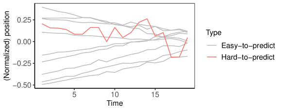
Figure 1: One-dimensional representations of 10 pedestrian trajectories, one of which is intrinsically less predictable.

The aforementioned limitations of marginal coverage have been acknowledged before. While achieving stronger theoretical guarantees in finite samples is generally unfeasible [41, 42], some approaches practically tend to work better in this regard than others. In particular, methods have been developed for regression [8, 43], classification [23, 44, 24], and sketching [45] to seek approximate conditional coverage guarantees stronger than (1).

2.3 Towards Approximate Conditional Coverage

The goal in this paper is to construct prediction bands that are valid not only for a large fraction of all trajectories but also with high probability for distinct “types” of trajectory. In our street crossing example, this means we would like to have valid coverage not only marginally but also conditional on some relevant features of the pedestrian. For example, one may want $\hat{C}^{(n+1)}$ to approximately satisfy

$$\mathbb{P}\left[Y_{t}^{(n+1)}\in\hat{C}_{t}(\bm{Y}^{(n+1)}),\;\forall t\mid\phi(\bm{Y}^{(n+1)})\right]\geq 1-\alpha,$$ (2)

where $\phi$ could represent the indicator of whether $\bm{Y}^{(n+1)}$ corresponds to an intoxicated pedestrian.

While there exist algorithms providing coverage conditional on a limited set of discrete features [46], our challenge exceeds the capabilities of available approaches. One issue is that our relevant features might not be directly observable. For example, an autonomous vehicle might only detect a pedestrian’s movements in real time, lacking broader contextual information about that person. Therefore, our problem requires an innovative approach.

2.4 Preview of Main Contributions

We present a novel method for constructing prediction bands for (multi-dimensional) trajectories. This method, called Conformalized Adaptive Forecaster for Heterogeneous Trajectories (CAFHT), guarantees simultaneous marginal coverage in the sense of (1) and typically achieves higher conditional coverage (2) compared to existing approaches. Further, our method produces prediction bands that are guaranteed to be valid most of the time even for worst-case trajectories, as long as the latter are sufficiently long.

Figure 2 offers a glimpse into the effectiveness of CAFHT applied to the pedestrian trajectories from Figure 1. Our method’s advantage over state-of-the-art techniques [17, 39] lies in its ability to automatically generate narrower bands for easier trajectories and wider ones for harder paths. As shown through extensive experiments, this leads to more useful uncertainty estimates with higher conditional coverage. In contrast, existing methods struggle to accommodate heterogeneity, often resulting in uniform prediction bands for all trajectories.

Figure 2: Conformal forecasting bands constructed using different methods, for the heterogeneous pedestrian trajectories from Figure 1. All methods guarantee simultaneous marginal coverage at the 90% level. Our method (CAFHT) can also automatically adapt to the unpredictability of each trajectory. Note that, in this case, the CFRNN bands are very wide and span from -1 to 1 at all times.

In the next section, we explain how our approach merges traditional split-conformal inference with online conformal prediction methods [20, 21, 22]. Originally designed for single-series forecasting, these methods can be repurposed in our setting to construct flexible prediction bands, automatically adapting to the unpredictability of each trajectory. For simplicity, we begin by presenting an implementation of our method that builds upon ACI [20], although other approaches such as the PID method of [22] can be seamlessly accommodated (see Section 3.7).

3 Methodology

3.1 Training a Black-Box Forecasting Model

The preliminary step in our CAFHT method consists of randomly partitioning the data set $\mathcal{D}$ into two distinct subsets of trajectories, $\mathcal{D}_{\text{train}}$ and $\mathcal{D}_{\text{cal}}$. The subset $\mathcal{D}_{\text{train}}$ is used to train a forecasting model $\hat{g}$. This model could be almost anything, including a long short-term memory network (LSTM) [47, 48], a transformer network [49, 50], or a traditional autoregressive moving average model [51]. Our only assumption regarding $\hat{g}$ is that it is able to generate point predictions for future steps based on partial observations from a new time series.

In this paper, we choose an LSTM model for demonstration and focus on one-step-ahead predictions. While the ability of CAFHT to guarantee simultaneous marginal coverage does not depend on the forecasting accuracy of $\hat{g}$, more accurate models generally tend to yield more informative conformal predictions [52].

3.2 Initializing the Adaptive Prediction Bands

After training the forecaster $\hat{g}$ on the data in $\mathcal{D}_{\text{train}}$, our method will convert its one-step-ahead point predictions for any new trajectory $\bm{Y}$ into suitable prediction bands. This is achieved by applying the Adaptive Conformal Inference algorithm (ACI) of [20]. For simplicity, we begin by focusing on the special case of one-dimensional trajectories ($d=1$). An extension of our solution to higher-dimensional trajectories is deferred to Section 3.6.

ACI was designed to generate one-step-ahead forecasts for a single one-dimensional time series, without requiring a pre-trained forecaster $\hat{g}$. In the single-series framework, [20] suggested training $\hat{g}$ in an online manner. In our setting, where we have access to multiple trajectories from the same population, it is logical to pre-train it. In any case, pre-training does not exclude the potential for further online updates of $\hat{g}$ with each subsequent one-step-ahead prediction. However, to simplify the notation, our discussion now focuses on a static model.

A review of ACI [20] can be found in Appendix A. Here, we briefly highlight two critical aspects of that algorithm. Note that the main ideas of our method can also be straightforwardly applied in combinations with other variations of the ACI method, as shown in Section 3.7.

Firstly, the ACI algorithm involves a “learning rate” parameter $\gamma>0$, controlling the adaptability of the prediction bands to the evolving time series. The adjustment mechanism operates as follows: at each time $t$, ACI modifies the width of the upcoming prediction interval for $Y^{(t+1)}$. If the previous interval failed to encompass $Y^{(t)}$, the next interval is expanded; conversely, if it was sufficient, the next interval is narrowed. Thus, larger values of $\gamma$ result in more substantial adjustments at each time step. In contrast, lower values of $\gamma$ generally lead to “smoother” prediction bands.

Secondly, the width of the ACI prediction band is also influenced by a parameter $\alpha\in(0,1)$, which represents the nominal level of the method. The design of the ACI algorithm aims to ensure that, over an extended period, the generated prediction bands will accurately contain the true value of $Y_{t}$ approximately a $1-\alpha$ fraction of the time. Consequently, a smaller $\alpha$ leads to broader bands.

Within our context, ACI is useful to transform the point predictions of $\hat{g}$ into uncertainty-aware prediction bands, but it is not satisfactory on its own. Firstly, it is not always clear how to choose a good learning rate. Secondly, the ACI prediction bands lack finite-sample guarantees. Specifically, they do not guarantee simultaneous marginal coverage (1). Our method overcomes these limitations as follows.

3.3 Calibrating the Adaptive Prediction Bands

We now discuss how to calibrate the ACI prediction bands discussed in the previous section to achieve simultaneous marginal coverage (1). For simplicity, we begin by taking the learning rate parameter $\gamma$ as fixed. We will then discuss later how to optimize the choice of $\gamma$ in a data-driven way.

Let $\hat{C}^{\text{ACI}}(\bm{Y}^{(i)},\gamma)=[\hat{\ell}^{\text{ACI}}(\bm{Y}^{(i)},\gamma),\hat{u}^{\text{ACI}}(\bm{Y}^{(i)},\gamma)]$ denote the prediction band constructed by ACI, with learning rate $\gamma$ and level $\alpha_{\mathrm{ACI}}\in(0,1)$, for each calibration trajectory $i\in\mathcal{D}_{\text{cal}}$. Note that this band is constructed one step at a time, based on the point predictions of $\hat{g}$ at each step $t\in[T]$ and past observations of $Y_{s}^{(i)}$ for all $s<t$; see Appendix A for further details on ACI. We will refer to the cross-sectional prediction interval identified by this band at time $t\in[T]$ as $\hat{C}^{\text{ACI}}_{t}(\bm{Y}^{(i)},\gamma)=[\hat{\ell}^{\text{ACI}}_{t}(\bm{Y}^{(i)},\gamma),\hat{u}^{\text{ACI}}_{t}(\bm{Y}^{(i)},\gamma)]$.

Our method will transform these ACI bands, which can only achieve a weaker notion of asymptotic average coverage because they do not leverage any exchangeability, into simultaneous prediction bands satisfying (2). For each $i\in\mathcal{D}_{\text{cal}}$, CAFHT evaluates a conformity score $\hat{\epsilon}_{i}(\gamma)$:

$$\begin{split}\hat{\epsilon}_{i}(\gamma):=\max_{t\in[T]}\Biggr{\{}\max\Biggr{\{}&\left[\hat{\ell}^{\text{ACI}}_{t}(\bm{Y}^{(i)},\gamma)-Y_{t}^{(i)}\right]_{+},\left[Y_{t}^{(i)}-\hat{u}^{\text{ACI}}_{t}(\bm{Y}^{(i)},\gamma)\right]_{+}\Biggr{\}}\Biggr{\}},\end{split}$$ (3)

where $[x]_{+}:=\max(0,x)$ for any $x\in\mathbb{R}$. Intuitively, $\hat{\epsilon}_{i}(\gamma)$ measures the largest margin by which $\hat{C}^{\text{ACI}}(\bm{Y}^{(i)},\gamma)$ should be expanded in both directions to simultaneously cover the entire trajectory $\bm{Y}^{(i)}$ from $t=1$ to $t=T$. This is inspired by the method of [8] for quantile regression, although one difference is that their scores may be negative. Other choices of conformity scores are also possible in our context, however, as discussed in Section 3.5.

Let $\hat{Q}(1-\alpha,\gamma)$ denote the $\lceil(1-\alpha)(1+|\mathcal{D}_{\text{cal}}|)\rceil$-th smallest value of $\hat{\epsilon}_{i}(\gamma)$ among $i\in\mathcal{D}_{\text{cal}}$. CAFHT constructs a prediction band $\hat{C}(\bm{Y}^{(n+1)},\gamma)$ for $\bm{Y}^{(n+1)}$, one step at a time, as follows. Let $\hat{C}^{\text{ACI}}_{t}(\bm{Y}^{(n+1)},\gamma)$ denote the ACI prediction interval for $Y_{t}^{(n+1)}$ at time $t\in[T]$. (Recall this depends on $\hat{g}$ and $\bm{Y}_{s}^{(n+1)}$ for all $s<t$.) Then, define the interval

$$\begin{split}\hat{C}_{t}(\bm{Y}^{(n+1)},\gamma)&=\bigg{[}\hat{\ell}^{\text{ACI}}_{t}(\bm{Y}^{(n+1)},\gamma)-\hat{Q}(1-\alpha,\gamma),\hskip 5.0pt\hat{u}^{\text{ACI}}_{t}(\bm{Y}^{(n+1)},\gamma)+\hat{Q}(1-\alpha,\gamma)\bigg{]}.\end{split}$$ (4)

Our prediction band $\hat{C}(\bm{Y}^{(n+1)},\gamma)$ for one-step-ahead forecasting is then obtained by concatenating the intervals in (4) for all $t\in[T]$. More compactly, we can write $\hat{C}(\bm{Y}^{(n+1)},\gamma)=\hat{C}^{\text{ACI}}(\bm{Y}^{(n+1)},\gamma)\pm\hat{Q}(1-\alpha,\gamma)$.

The next result establishes finite-sample simultaneous coverage guarantees for this method.

Theorem 1.

Assume that the calibration trajectories in $\mathcal{D}_{\text{cal}}$ are exchangeable with $\bm{Y}^{(n+1)}$. Then, for any $\alpha\in(0,1)$, the prediction band output by CAFHT, applied with fixed parameters $\alpha$, $\alpha_{\mathrm{ACI}}$, and $\gamma$, satisfies (1).

The proof of Theorem 1 is relatively simple and can be found in Appendix B. We remark that this guarantee holds at the desired level $\alpha$ regardless of the value of the ACI parameter $\alpha_{\mathrm{ACI}}$. However, it is typically intuitive to set $\alpha_{\mathrm{ACI}}=\alpha$. A notable advantage of this choice is that it leaves us with the challenge of tuning only one ACI parameter, $\gamma$.

Further, it is important to note that CAFHT can only expand the ACI prediction bands, since its conformity scores are non-negative. Thus, our method retains the ACI guarantee of asymptotic average coverage at level $1-\alpha$ [20], almost surely for any trajectory $\bm{Y}^{(n+1)}$:

$$\underset{T\rightarrow\infty}{\lim}\frac{1}{T}\sum_{t=1}^{T}\mathbb{I}[Y_{t}\notin\hat{C}_{t}(\bm{Y}^{(n+1)},\gamma)]\overset{\mathrm{a.s.}}{=}\alpha.$$ (5)

See Appendix A for details about how ACI achieves (5).

3.4 Data-Driven Parameter Selection

The ability of the ACI algorithm to produce informative prediction bands can sometimes be sensitive to the choice of the learning rate $\gamma$ [20, 22]. This leads to a question: how can we select $\gamma$ in a data-driven manner? In our scenario, which involves multiple relevant trajectories from the same population, addressing this tuning challenge is somewhat simpler than in the original single-series context for which the ACI algorithm was designed. Nonetheless, careful consideration is still required in the tuning process of $\gamma$, as we discuss next.

As a naive approach, one may feel tempted to apply the CAFHT method described above using different learning rates, with the idea of then cherry-picking the value of $\gamma$ leading to the most appealing prediction bands. Unsurprisingly, however, such an unprincipled approach would invalidate the coverage guarantee because it breaks the exchangeability between the test trajectory and the calibration data. This issue is closely related to problems of conformal prediction after model selection previously studied by [53] and [54]. Therefore, we propose two alternative solutions inspired by their works.

The simplest approach to explain involves an additional data split. Let us randomly partition $\mathcal{D}_{\text{cal}}$ into two subsets of trajectories, $\mathcal{D}_{\text{cal}}^{1}$ and $\mathcal{D}_{\text{cal}}^{2}$. The trajectories in $\mathcal{D}_{\text{cal}}^{1}$ can be utilized to select a good choice of $\gamma$ in a data-driven way. In particular, we seek the value of $\gamma$ leading to the most informative prediction bands—a goal that can be quantified by minimizing the average width of our prediction bands produced for the trajectories in $\mathcal{D}_{\text{cal}}^{1}$. Then, the calibration procedure described in Section 3.3 will be applied using only the data in $\mathcal{D}_{\text{cal}}^{2}$ instead of the full $\mathcal{D}_{\text{cal}}$. The fact that the selection of $\gamma$ does not depend on the calibration trajectories in $\mathcal{D}_{\text{cal}}^{2}$ means that $\gamma$ can be essentially regarded as fixed, and therefore our output bands enjoy the marginal simultaneous coverage guarantee of Theorem 1. This version of our CAFHT method is outlined in Algorithm 1. The parameter tuning module of this procedure is summarized by Algorithm 2 in Appendix C, for lack of space.

Algorithm 1 CAFHT

1:  Input: A pre-trained forecaster $\hat{g}$ producing one-step-ahead predictions; calibration trajectories $\mathcal{D}_{\text{cal}}$; the initial position $Y_{0}^{(n+1)}$ of a test trajectory $\bm{Y}^{(n+1)}$; the desired nominal level $\alpha\in(0,1)$; a grid of candidate learning rates $\{\gamma_{1},\dots,\gamma_{L}\}$.

2:  Randomly split $\mathcal{D}_{\text{cal}}$ into $\mathcal{D}_{\text{cal}}^{1}$ and $\mathcal{D}_{\text{cal}}^{2}$.

3:  Select a learning rate $\hat{\gamma}\in\{\gamma_{1},\ldots,\gamma_{L}\}$, applying Algorithm 2 using the trajectory data in $\mathcal{D}_{\text{cal}}^{1}$.

4:  Construct $\hat{C}^{\text{ACI}}(\bm{Y}^{(i)},\hat{\gamma})$ using ACI, for $i\in\mathcal{D}_{\text{cal}}^{2}$.

5:  Evaluate $\hat{\epsilon}_{i}(\hat{\gamma})$ using (3), for $i\in\mathcal{D}_{\text{cal}}^{2}$.

6:  Compute the empirical quantile $\hat{Q}(1-\alpha,\hat{\gamma})$.

7:  for $t\in[T]$ do

8:     Compute $\hat{C}^{\text{ACI}}_{t}(\bm{Y}^{(n+1)},\hat{\gamma})$ with ACI, using the past of the test trajectory $(Y_{0}^{(n+1)},Y_{1}^{(n+1)},\ldots,Y_{t-1}^{(n+1)})$.

9:     Compute a prediction interval $\hat{C}_{t}(\bm{Y}^{(n+1)},\hat{\gamma})$ for the next step, using (4).

10:     Observe the next step of the trajectory, $Y_{t}^{(n+1)}$.

11:  end for

12:  Output: An online prediction band $\hat{C}(\bm{Y}^{(n+1)})$.

Alternatively, it is also possible to carry out the selection of $\hat{\gamma}$ in a rigorous way without splitting $\mathcal{D}_{\text{cal}}$. However, this would require replacing the empirical quantile $\hat{Q}(1-\alpha,\hat{\gamma})$ in the CAFHT method with a more conservative quantity $\hat{Q}(1-\alpha^{\prime},\hat{\gamma})$, where the value of $\alpha^{\prime}<\alpha$ depends on the number $L$ of candidate parameter values considered. We refer to Appendix D for further details.

3.5 CAFHT with Multiplicative Scores

A potential shortcoming of Algorithm 1 is that it can only add a constant margin of error to the prediction band constructed by the ACI algorithm. While straightforward, this approach may not be always optimal. In many cases, it would seem more natural to utilize a multiplicative error. The rationale behind this is intuitive: trajectories that are inherently more unpredictable, resulting in wider ACI prediction bands, may necessitate larger margins of error to ensure valid simultaneous coverage. This concept can be seamlessly integrated into the CAFHT method by replacing the conformity scores initially outlined in (3) with these:

$$\begin{split}\tilde{\epsilon}_{i}(\gamma)=\max_{t\in T}\Biggr{\{}\max\Biggr{\{}&\frac{\left[\hat{\ell}^{\text{ACI}}_{t}(\bm{Y}^{(i)},\gamma)-Y_{t}^{(i)}\right]_{+}}{|\hat{C}^{\text{ACI}}_{t}(\bm{Y}^{(i)},\gamma)|},\frac{\left[Y_{t}^{(i)}-\hat{u}^{\text{ACI}}_{t}(\bm{Y}^{(i)},\gamma)\right]_{+}}{|\hat{C}^{\text{ACI}}_{t}(\bm{Y}^{(i)},\gamma)|}\Biggr{\}}\Biggr{\}}.\end{split}$$ (6)

Then, the counterpart of Equation (4) becomes

$$\begin{split}\hat{C}(\bm{Y}^{(n+1)},\gamma)&=\hat{C}^{\text{ACI}}(\bm{Y}^{(n+1)},\gamma)\pm\tilde{Q}(1-\alpha,\gamma)\cdot|\hat{C}^{\text{ACI}}(\bm{Y}^{(n+1)},\gamma)|,\end{split}$$

where $\tilde{Q}(1-\alpha,\gamma)$ is the $\lceil(1-\alpha)(1+|\mathcal{D}_{\text{cal}}|)\rceil$-th smallest value in $\{\tilde{\epsilon}_{i}(\gamma),i\in\mathcal{D}_{\text{cal}}\}$.

At this point, it is easy to prove that the prediction bands obtained produced by CAFHT with these multiplicative conformity scores still enjoy the same marginal simultaneous coverage guarantee established by Theorem 1.

3.6 Extension to Multi-Dimensional Trajectories

The problem of forecasting trajectories with $d>1$ (e.g., a two-dimensional walk), can be addressed with an intuitive extension of CAFHT. In fact, ACI extends naturally to the multidimensional case and the first component of our method that requires some special care is the computation of the empirical quantile $\hat{Q}(1-\alpha,\hat{\gamma})$. Yet, even this obstacle can be overcome quite easily. Consider evaluating a vector-valued version of the additive scores from (3):

$$\begin{split}\hat{\epsilon}_{ij}(\gamma):=\max_{t\in[T]}\Biggr{\{}\max\Biggr{\{}&\left[\hat{\ell}^{\text{ACI}}_{t,j}(\bm{Y}^{(i)},\gamma)-Y_{t,j}^{(i)}\right]_{+},\left[Y_{t,j}^{(i)}-\hat{u}^{\text{ACI}}_{t,j}(\bm{Y}^{(i)},\gamma)\right]_{+}\Biggr{\}}\Biggr{\}},\end{split}$$ (7)

for each dimension $j\in[d]$. Then, we can recover a one-dimensional problem prior to computing $\hat{Q}(1-\alpha,\hat{\gamma})$ by taking (for example) the maximum value of $\hat{\epsilon}_{ij}(\gamma)$; i.e., $\hat{\epsilon}_{i}^{\infty}(\gamma)=\max_{j\in[d]}\hat{\epsilon}_{ij}(\gamma)$. Ultimately, each $\hat{C}_{t}(\bm{Y}^{(n+1)},\gamma)$ is obtained by applying (4) with $\hat{Q}(1-\alpha,\hat{\gamma})$ defined as the $\lceil(1-\alpha)(1+|\mathcal{D}_{\text{cal}}|)\rceil$-th smallest value of $\hat{\epsilon}_{i}^{\infty}(\gamma)$.

We conclude this section by remarking that this general idea could also be implemented using the multiplicative conformity scores described in Section 3.5, as well as by using different dimension reduction functions in (3). For example, one may consider replacing the infinity-norm in (3) with an $\ell^{2}$ norm, leading to a “spherical” margin of error around the ACI prediction bands instead of a “square” one.

3.7 Leveraging PID Prediction Bands Instead of ACI

CAFHT is not heavily reliant on the specific mechanics of ACI. The crucial aspect of ACI is its capability to transform black-box point forecasts into prediction bands that approximately mirror the unpredictability of each trajectory. Thus, our method can integrate with any variation of ACI.

Some of our demonstrations in Appendix E include an alternative implementation of CAFHT that employs the PID algorithm of [22] instead of ACI. To minimize computational demands, our demonstrations will primarily utilize the quantile tracking feature of the original PID method. This simplified version of PID is influenced only by a learning rate parameter $\gamma$, similar to ACI.

4 Numerical Experiments

4.1 Setup and Benchmarks

This section demonstrates the empirical performance of our method. We focus on applying CAFHT with multiplicative scores, based on the ACI algorithm, and tuning the learning rate through data splitting. Additional results pertaining to different implementations of CAFHT are in Appendix E. In all experiments, the candidate values for the ACI learning rate parameter $\gamma$ range from $0.001$ to $0.1$ at increments of $0.01$, and from $0.2$ to $0.9$ at increments of $0.1$.

The CAFHT method is compared with two benchmark approaches that also provide simultaneous marginal coverage (1). The first one is the Conformal Forecasting Recurrent Neural Network (CFRNN) approach of [17], which relies on a Bonferroni correction for multiple testing. In particular, the CFRNN method produces a prediction band satisfying (1) for a trajectory of length $T$ by separately computing $T$ conformal prediction intervals at level $\alpha/T$, one for each time step, each obtained using regression techniques typical to the regression setting. An advantage of this approach is that it is conceptually intuitive, but it can become quite conservative if $T$ is large.

The second benchmark is the Normalized Conformal Trajectory Predictor (NCTP) of [39]. This method is closer to ours but utilizes different scores and does not leverage ACI to adapt to heterogeneity. In short, NCTP directly takes as input a forecaster $\hat{g}$ providing one-step-ahead point predictions $\hat{Y}^{(i)}_{t}$ and evaluates the scores $\hat{\epsilon}_{i}=\max_{t\in[T]}\{(|\hat{Y}^{(i)}_{t}-Y^{(i)}_{t}|)/\sigma_{t}\}$ for each $i\in\mathcal{D}_{\mathrm{cal}}$, where $\sigma_{t}$ are suitable data-driven normalization constants. This approach is similar to that of [40], which deviates only in the computation of the $\sigma_{t}$ constants, and it tends to work quite well if the trajectories are homogeneous.

For all methods, the underlying forecasting model is a recurrent neural network with 4 stacked LSTM layers followed by a linear layer. The learning rate is set equal to 0.001, for an AdamW optimizer with weight decay 1e-6. The models are trained for a total of 50 epochs, so that the mean squared error loss loss approximately converges.

Prior to the beginning of our analyses, all trajectories will be pre-processed with a batch normalization step based on $\mathcal{D}_{\mathrm{train}}$, so that all values lie within the interval $[-1,1]$. This is useful to ensure a numerically stable learning process and more easily interpretable performance measures.

In all experiments, we will evaluate the performance of the prediction bands in terms of their marginal simultaneous coverage (i.e., the proportion of test trajectories entirely contained within the prediction bands), the average width (over all times $t\in[T]$ and all test trajectories), and the simultaneous coverage conditional on a trajectory being “hard-to-predict”, as made more precise below.

4.2 Synthetic Trajectories

We begin by considering univariate ($d=1)$ synthetic trajectories generated from an autoregressive (AR) model, $X_{t}=0.9X_{t-1}+0.1X_{t-2}-0.2X_{t-3}+\epsilon_{t}$, where $\epsilon_{t}\sim N(0,\sigma_{t}^{2})$, for all $t\in[T]$ with $T=100$. Similar to [17], we consider two noise profiles: a dynamic profile in which $\sigma_{t}^{2}$ is increasing with time, and a static profile in which $\sigma_{t}^{2}$ is constant. The results based on the dynamic profile are presented here, while the others are discussed in Appendix E. To make the problem more interesting, we ensure that some trajectories are intrinsically more unpredictable than the others. Specifically, in the dynamic noise setting, we set $\sigma_{t}^{2}=t\cdot k$, with $k=10$, for a fraction $\delta=0.1$ of the trajectories, while $\sigma_{t}^{2}=t$ for the remaining ones.

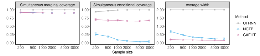
Figure 3: Performance on simulated heterogeneous trajectories of prediction bands constructed by different methods, as a function of the total number of training and calibration trajectories. All methods achieve 90% simultaneous marginal coverage. Our method (CAFHT) leads to more informative bands with lower average width and higher conditional coverage. The error bars indicate 2 standard errors.

Figure 3 summarizes the performance of the three methods as a function of the number of trajectories in $\mathcal{D}$, which is varied between 200 and 10,000. The results are averaged over 500 test trajectories and 100 independent experiments. See Table 1 in Appendix E for standard errors. In each case, $75\%$ of the trajectories are used for training and the remaining $25\%$ for calibration. Our method utilizes 50% of the calibration trajectories to select the ACI learning rate $\gamma$.

All methods attain 90% simultaneous marginal coverage, aligning with theoretical predictions. Notably, CAFHT yields the most informative bands, characterized by the narrowest average width and higher conditional coverage compared to NCTP. This can be explained by the fact that NCTP is not designed to account for the varying noise levels inherent in different trajectories. Consequently, NCTP generates less adaptive bands, too wide for the simpler trajectories and too narrow for the harder ones. In contrast, CFRNN tends to produce unnecessarily wide bands for all trajectories, a consequence of its rigid way of dealing with time dependencies through a Bonferroni correction.

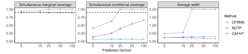
Figure 4: Performance on simulated heterogeneous trajectories of conformal prediction bands constructed by different methods, as a function of the prediction horizon. Other details are as in Figure 3.

Figure 4 summarizes the results of similar experiments investigating the performances of different methods as a function of the prediction horizon $T$, which is varied between 5 and 100; see Table 2 in Appendix E for the corresponding standard errors. Here, the number of trajectories in $\mathcal{D}$ is fixed equal to 2000. The results highlight how CFRNN becomes more conservative as $T$ increases. By contrast, NCTP produces relatively narrower bands but also achieves the lowest conditional coverage. Meanwhile, our CAFHT method again yields the most informative prediction bands, with low average width and high conditional coverage.

Appendix E describes additional experimental results that are qualitatively consistent with the main findings. These supplementary experiments investigate the effects of the data dimensionality (Figure 6 and Table 3), of the proportion of hard trajectories (Figure 7 and Table 4), and evaluate the robustness of different methods against distribution shifts (Figure 8 and Table 5). Additionally, these experiments are replicated using synthetic data from an AR model with a static noise profile; see Figures 9–13 and Tables 6–10.

Furthermore, we conducted several experiments to investigate the performance of various implementations of our method. Figures 14–18 and Tables 11–15 focus on comparing alternative model selection approaches while applying the multiplicative conformity scores defined in Equation (6). Figures 19–23 and Tables 16–20 summarize similar experiments based on the additive scores defined in Equation (3).

4.3 Pedestrian Trajectories

We now apply the three methods to forecast pedestrian trajectories generated from the ORCA simulator [55]. The data include 2-dimensional position measurements for 1,291 pedestrians, tracked over $T=20$ time steps. To make the problem more challenging, we introduce dynamic noise to the trajectories of 10% of randomly selected pedestrians, making their paths more unpredictable. Figure 1 plots ten representative trajectories.

All trajectories are normalized as in the previous section, and we train the same LSTM for 50 epochs. In each experiment, the test set consists of 291 randomly chosen trajectories. All results are averaged over 100 runs.

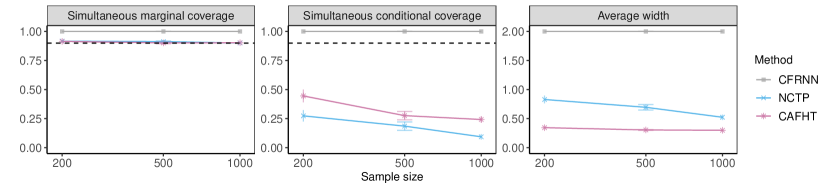
Figure 5: Performance on heterogeneous pedestrian trajectories of conformal prediction bands constructed by different methods, as a function of the total number of training and calibration trajectories. Other details are as in Figure 3.

Figure 5 compares the performances of different methods as a function of the sample size used for training and calibration, which is varied between 200 and 1000. Again, all methods attain $90\%$ simultaneous marginal coverage, but CAFHT produces the most informative bands, with relatively narrow width and higher conditional coverage compared to NCTP. Meanwhile, CFRNN leads to very conservative bands, as in the previous section. See Table 21 in Appendix E for further details.

Additional numerical experiments are summarized in Appendix E. Figure 24 and Table 22 investigate the effect of varying the noise level, setting $\sigma_{t}^{2}\propto t\cdot\text{noise level}$ (varied from 5 to 50) for the hard trajectories and $\sigma_{t}^{2}\propto t$ for the easy ones. We then refer to Figures 25–28 and Tables 23–26 for a comparative analysis of different implementations of our methods under varying sample sizes and noise levels, using both multiplicative and additive conformity scores.

5 Discussion

This work opens several directions for future research. On the theoretical side, one may want to understand the conditions under which our method can asymptotically achieve optimal prediction bands in the limit of large sample sizes, potentially drawing inspiration from [52] and [56]. Moreover, there are several potential ways to further enhance our method and address some of its remaining limitations. For example, it could be adapted to provide even stronger types of coverage guarantees beyond those considered in this paper, reduce algorithmic randomness caused by data splitting [57, 58, 59], and increase adaptability to potential distribution shifts [25]. Lastly, it would be especially interesting to apply this method in real-world motion planning scenarios.

Software implementing the algorithms and data experiments are available online at https://github.com/FionaZ3696/CAFHT.git.

Acknowledgements

The authors thank the Center for Advanced Research Computing at the University of Southern California for providing computing resources to carry out numerical experiments. M. S. and Y. Z. are supported by NSF grant DMS 2210637. M. S. is also supported by an Amazon Research Award.

Appendix A Further Details on the ACI Algorithm

A.1 Background on ACI

In this section, we briefly review some relevant components of the adaptive conformal inference (ACI) method introduced by [20] in the context of forecasting a single time series. The goal of ACI is to construct prediction bands in an online setting, while accounting for possible changes in the data distribution across different times. Specifically, ACI is designed to create prediction bands with a long-term average coverage guarantee. Intuitively, this guarantee means that, for an indefinitely long time series, a sufficiently large proportion of the series should be contained within the output band. This objective is notably distinct from the one investigated in our paper. However, since our method builds upon ACI, it can be useful to recall some relevant technical details of the latter method.

In the online learning setting considered by [20], one observes covariate-response pairs $\{(X_{t},Y_{t})\}_{t\in\mathbb{N}}\subset\mathbb{R}^{d}\times\mathbb{R}$ in a sequential fashion. At each time step $t\in\mathbb{N}$, the goal is to form a prediction set $\hat{C}_{t}$ for $Y_{t}$ using the previously observed data $\{(X_{r},Y_{r})\}_{1\leq r\leq t-1}$ as well as the new covariates $X_{t}$. Given a target coverage level $\alpha\in(0,1)$, the constructed prediction set should guarantee that, over long time, at least $100(1-\alpha)\%$ of the time $Y_{t}$ lies within the set.

Recall that standard split-conformal prediction methods require a calibration dataset $\mathcal{D}_{\text{cal}}\subseteq\{(X_{r},Y_{r})\}_{1\leq r\leq t-1}$ that is independent of the data used to fit the regression model. The standard approach involves constructing a prediction set as $\hat{C}_{t}(\alpha)=\{y:S(X_{t},y)\leq\hat{Q}(1-\alpha)\}$, where $S(X_{t},y)$ is a score that measures how well $y$ conforms with the prediction of the fitted model. For example, if we denote the fitted model as $\hat{g}$, a classical example of scoring function would be $S(X_{t},y)=|\hat{g}(X_{t})-y|$. Then, in general, the score $S(X_{t},y)$ is compared to a suitable empirical quantile, $\hat{Q}(1-\alpha)$, of the analogous scores evaluated on the calibration data: $\hat{Q}(1-\alpha)=\inf\{s:(|\mathcal{D}_{\text{cal}}|^{-1}\sum_{(X_{r},Y_{r})\in\mathcal{D}_{\text{cal}}}\mathbbm{1}_{\{S(X_{r},Y_{r})\leq s\}})\geq 1-\alpha\}$. If the observations taken at different times are not exchangeable with one another, however, standard conformal prediction algorithms cannot achieve valid coverage. This is where ACI comes into play.

The core concept of ACI involves dynamically updating the functions $\hat{g}$, $S(\cdot)$, and $\hat{Q}(\cdot)$ at each time step, utilizing newly acquired data. Concurrently, ACI modifies the nominal miscoverage target level $\alpha_{t}$ of its conformal predictor for each time increment. The purpose of adjusting the $\alpha$ level at each time step is to calibrate future predictions to be more or less conservative depending on their empirical performance in covering past values of the time series. For instance, if a prediction band is found to be excessively broad, it will be narrowed in subsequent steps, and the opposite applies if it’s too narrow. This strategy enables ACI to continuously adapt to potential dependencies and distribution changes within the time series, maintaining relevance and accuracy in an online context. Specifically, ACI employs the following $\alpha$-update rule:

$$\alpha_{t+1}=\alpha_{t}+\gamma(\alpha-\text{err}_{t}),$$

where

$$\text{err}_{t}=\begin{cases}1,&\text{ if }Y_{t}\notin\hat{C}^{\text{ACI}}_{t}(\alpha_{t}),\\ 0,&\text{ otherwise}.\end{cases},$$

and $\hat{C}^{\text{ACI}}_{t}(\alpha_{t})=\{y:S_{t}(X_{t},y)\leq\hat{Q}_{t}(1-\alpha_{t})\}$. Equivalently,

$$\hat{C}^{\text{ACI}}_{t}(\alpha_{t})=[\hat{\ell}^{\text{ACI}}_{t},\hat{u}^{\text{ACI}}_{t}]=[\hat{g}(X_{t})-\hat{Q}_{t}(1-\alpha_{t}),\hat{g}(X_{t})+\hat{Q}_{t}(1-\alpha_{t})].$$

The hyperparameter $\gamma>0$ controls the magnitude of each update step. Intuitively, a larger $\gamma$ means that ACI can rapidly adjust to observed changes in the data distribution. However, this may come at the expense of increased instability in the prediction bands. Consequently, the ideal value of $\gamma$ tends to be specific to the application at hand, requiring careful consideration to balance responsiveness and stability. This is why our CAFHT method involves a data-driven parameter tuning component.

The main theoretical finding established by [20] is that ACI always attains valid long-term average coverage. Notably, this result is achieved without the necessity for any assumptions regarding the distribution of the unique time series in question. More precisely, with probability one,

$$\left|\frac{1}{T}\sum_{t=1}^{T}\text{err}_{t}-\alpha\right|\leq\frac{\max(\alpha_{1},1-\alpha_{1})+\gamma}{T\gamma},$$

which implies

$$\underset{T\rightarrow\infty}{\lim}T^{-1}\sum_{t=1}^{T}\text{err}_{t}\overset{\mathrm{a.s.}}{=}\alpha.$$

This result is not essential for proving our simultaneous marginal coverage guarantee, but it offers an intuitive rationale for our methodology. Indeed, the capacity of ACI to adaptively encompass the inherent variability in each time series is key to our method’s enhanced conditional coverage compared to other conformal prediction approaches for multi-series forecasting. Further, our method inherits the same long-term average coverage property of ACI because it can only expand the prediction bands of the latter.

In this paper, we implement ACI without re-training the forecasting model $\hat{g}$ at each step. This approach is viable due to our access to additional “training” time series data from the same population, and it aids in diminishing the computational cost of our numerical experiments. Nonetheless, our methodology is flexible enough to incorporate ACI with periodic re-training, aligning with the practices suggested by [20] and the very recent related PID method of [22].

A.2 Warm Starts

As originally designed, ACI primarily aimed at achieving asymptotic coverage in the limit of a very long trajectory, sometimes tolerating very narrow prediction intervals in the initial time steps. However, we have observed that this behavior can negatively impact the performance of our method in finite-horizon scenarios. To address this issue, we introduce in this paper a simple warm-start approach for ACI. This involves incorporating artificial conformity scores at the start of each trajectory. These scores are generated as uniform random noise, with values falling within the range of observed residuals in the training dataset. Consequently, ACI typically begins with a wider interval for its first forecast. Importantly, this modification does not affect the long-term asymptotic properties of ACI when applied to a single trajectory, nor does it impact our guarantee of finite-sample simultaneous marginal coverage. However, it often results in more informative (narrower) prediction bands.

The solution described above is applied in our experiments using 5 warm-start scores, denoted as $\hat{\epsilon}_{-4},\dots,\hat{\epsilon}_{0}$, and setting the initial value of $\alpha_{-4}$ equal to 0.1. A similar warm-start approach is also utilized when we apply the PID algorithm of [22] instead of ACI. However, for the algorithm the warm start simply consists of setting the initial quantile $q_{0}$ equal to the $(1-\alpha)$-th quantile evaluated on the empirical distribution of scores computed using the training set.

Appendix B Proof of Theorem 1

Proof of Theorem 1.

The proof follows directly from the exchangeability of the conformity scores, as it is often the case for split-conformal prediction methods. Denote $\hat{\epsilon}_{n+1}(\gamma)$ the conformity score of the test trajectory $\bm{Y}^{(t+1)}$ evaluated using the ACI prediction band constructed with step size $\gamma$. For any fixed $\alpha$ and $\gamma>0$, we have that $Y_{t}^{(n+1)}\in\hat{C}^{(n+1)}_{t}\forall t\in[T]$ if and only if $\hat{\epsilon}_{n+1}(\gamma)\leq\hat{Q}(1-\alpha,\gamma)$, where $\hat{Q}(1-\alpha,\gamma)$ is the $\lceil(1-\alpha)(1+|\mathcal{D}_{\text{cal}}|)\rceil$-th smallest value of $\hat{\epsilon}_{i}(\gamma)$ for all $i\in\mathcal{D}_{\text{cal}}$. Since the test trajectory is exchangeable with $\mathcal{D}_{\text{cal}}$, its score $\hat{\epsilon}_{n+1}(\gamma)$ is also exchangeable with $\{\hat{\epsilon}_{i}(\gamma),i\in\mathcal{D}_{\text{cal}}\}$. Then by Lemma 1 in [8], it follows that $\mathbb{P}(Y_{t}^{(n+1)}\in\hat{C}^{(n+1)}_{t}\forall t\in[T])=\mathbb{P}(\hat{\epsilon}_{n+1}(\gamma)\leq\hat{Q}(1-\alpha,\gamma))\geq 1-\alpha$. ∎

Appendix C Algorithms

Algorithm 2 Model selection component of CAFHT

1:  Input: A pre-trained forecaster $\hat{g}$ producing one-step-ahead predictions; calibration trajectories $\mathcal{D}_{\text{cal}}^{1}$; a grid of candidate learning rates $\{\gamma_{1},\dots,\gamma_{L}\}$.

2:  for $\ell\in[L]$ do

3:     Construct $\hat{C}^{\text{ACI}}(\bm{Y}^{(i)},\gamma_{\ell})$ using ACI, for $i\in\mathcal{D}_{\text{cal}}^{1}$.

4:     Evaluate $\hat{\epsilon}_{i}(\gamma_{\ell})$ using (3), for $i\in\mathcal{D}_{\text{cal}}^{1}$.

5:     Compute $\hat{Q}(1-\alpha,\gamma_{\ell})$, the $(1-\alpha)(1+1/|\mathcal{D}_{\text{cal}}^{1}|)$-th quantile of $\{\hat{\epsilon}_{i}(\gamma_{\ell}),i\in\mathcal{D}_{\text{cal}}^{1}\}$.

6:     Construct $\hat{C}(\bm{Y}^{(i)},\gamma_{\ell})=(\hat{C}_{1}(\bm{Y}^{(i)},\gamma_{\ell}),\dots,\hat{C}_{T}(\bm{Y}^{(i)},\gamma_{\ell}))$ using (4) for $i\in\mathcal{D}_{\text{cal}}^{1}$.

7:  end for

8:  Pick $\hat{\gamma}$ such that,

$$\hat{\gamma}:=\operatorname*{arg\,min}_{\ell\in[L]}\text{AvgWidth}(C(\bm{Y}^{(i)},\gamma_{\ell})).$$ (8)

9:  Output: Selected learning rate parameter $\hat{\gamma}$.

Algorithm 3 CAFHT - multiplicative scores

1:  Input: A pre-trained forecaster $\hat{g}$ producing one-step-ahead predictions; calibration trajectories $\mathcal{D}_{\text{cal}}$; the initial position $Y_{0}^{(n+1)}$ of a test trajectory $\bm{Y}^{(n+1)}$; the desired nominal level $\alpha\in(0,1)$; a grid of candidate learning rates $\{\gamma_{1},\dots,\gamma_{L}\}$.

2:  Randomly split $\mathcal{D}_{\text{cal}}$ into $\mathcal{D}_{\text{cal}}^{1}$ and $\mathcal{D}_{\text{cal}}^{2}$.

3:  Select a learning rate $\hat{\gamma}\in\{\gamma_{1},\ldots,\gamma_{L}\}$, applying Algorithm 4 using the trajectory data in $\mathcal{D}_{\text{cal}}^{1}$.

4:  Construct $\hat{C}^{\text{ACI}}(\bm{Y}^{(i)},\hat{\gamma})$ using ACI, for $i\in\mathcal{D}_{\text{cal}}^{2}$.

5:  Evaluate $\hat{\epsilon}_{i}(\hat{\gamma})$ using (6), for $i\in\mathcal{D}_{\text{cal}}^{2}$.

6:  Compute the empirical quantile $\hat{Q}(1-\alpha,\hat{\gamma})$.

7:  for $t\in[T]$ do

8:     Compute $\hat{C}^{\text{ACI}}_{t}(\bm{Y}^{(n+1)},\hat{\gamma})$ with ACI, using the past of the test trajectory $(Y_{0}^{(n+1)},Y_{1}^{(n+1)},\ldots,Y_{t-1}^{(n+1)})$.

9:     Compute a prediction interval $\hat{C}_{t}(\bm{Y}^{(n+1)},\hat{\gamma})$ for the next step, using the multiplicative version of (4).

10:     Observe the next step of the trajectory, $Y_{t}^{(n+1)}$.

11:  end for

12:  Output: An online prediction band $\hat{C}(\bm{Y}^{(n+1)})$.

Algorithm 4 Model selection component of CAFHT - multiplicative scores

1:  Input: A pre-trained forecaster $\hat{g}$ producing one-step-ahead predictions; calibration trajectories $\mathcal{D}_{\text{cal}}^{1}$; a grid of candidate learning rates $\{\gamma_{1},\dots,\gamma_{L}\}$.

2:  for $\ell\in[L]$ do

3:     Construct $\hat{C}^{\text{ACI}}(\bm{Y}^{(i)},\gamma_{\ell})$ using ACI, for $i\in\mathcal{D}_{\text{cal}}^{1}$.

4:     Evaluate $\hat{\epsilon}_{i}(\gamma_{\ell})$ using (6), for $i\in\mathcal{D}_{\text{cal}}^{1}$.

5:     Compute $\hat{Q}(1-\alpha,\gamma_{\ell})$, the $(1-\alpha)(1+1/|\mathcal{D}_{\text{cal}}^{1}|)$-th quantile of $\{\hat{\epsilon}_{i}(\gamma_{\ell}),i\in\mathcal{D}_{\text{cal}}^{1}\}$

6:     Construct $\hat{C}(\bm{Y}^{(i)},\gamma_{\ell})=(\hat{C}_{1}(\bm{Y}^{(i)},\gamma_{\ell}),\dots,\hat{C}_{T}(\bm{Y}^{(i)},\gamma_{\ell}))$ for $i\in\mathcal{D}_{\text{cal}}^{1}$, using the multiplicative version of (4).

7:  end for

8:  Pick $\hat{\gamma}$ such that,

$$\hat{\gamma}:=\operatorname*{arg\,min}_{\ell\in[L]}\text{AvgWidth}(C(\bm{Y}^{(i)},\gamma_{\ell})).$$ (9)

9:  Output: Selected learning rate parameter $\hat{\gamma}$.

Appendix D Parameter Tuning for CAFHT Without Data Splitting

Here, we outline an alternate implementation of CAFHT which, in contrast to the primary method described in Section 3.4, obviates the need for additional subdivision of the calibration data in $\mathcal{D}_{\text{cal}}$ for selecting an optimal value of the ACI learning rate parameter $\gamma$. In essence, this version of CAFHT employs the same calibration dataset $\mathcal{D}_{\text{cal}}$ for both choosing $\hat{\gamma}$ and calibrating the conformal margin of error via $\hat{Q}(1-\alpha^{\prime},\hat{\gamma})$. It does so by using a judiciously selected $\alpha^{\prime}<\alpha$ to compensate for the selection step. Enabled by the theoretical results of [53] and [54], this method is outlined below by Algorithms 5–6 using additive conformity scores, and by Algorithms 7–8 using multiplicative conformity scores.

In the following, we will assume that the goal is for CAFHT to select a good $\hat{\gamma}$ from a list of $L$ candidate parameter values, $\gamma_{1}$, …, $\gamma_{L}$, for some fixed integer $L\geq 1$.

Using the DKW inequality, [53] proves that, when calibrating at the nominal level $\alpha$, a conformal prediction set $\hat{C}^{(n+1)}$ constructed after using the same calibration set $\mathcal{D}_{\text{cal}}$ to select the best model among $L$ candidates may have an inflated coverage rate in the following form:

$$\mathbb{P}(Y^{(n+1)}\in\hat{C}^{(n+1)})\geq\left(1+\frac{1}{|\mathcal{D}_{\text{cal}}|}\right)(1-\alpha)-\frac{\sqrt{\log(2L)/2}+c(L)}{\sqrt{|\mathcal{D}_{\text{cal}}|}},$$ (10)

where $c(L)$ is a constant that is generally smaller than $1/3$ and can be computed explicitly,

$$c(L)=\frac{\sqrt{2}Le^{-\log(2L)}}{\sqrt{\log(2L)}+\sqrt{\log(2L)+4/\pi}}.$$

This justifies applying CAFHT, without data splitting, using $\hat{Q}(1-\alpha^{\prime}_{\text{DKW}},\hat{\gamma})$ instead of $\hat{Q}(1-\alpha,\hat{\gamma})$, where

$$\alpha^{\prime}_{\text{DKW}}=1-\frac{1-\alpha+\text{err}}{1+1/|\mathcal{D}_{\text{cal}}|}, \text{err}=\frac{\sqrt{\log(2L)/2}+c(L)}{\sqrt{|\mathcal{D}_{\text{cal}}|}}.$$

A further refinement of this approach was proposed by [54], which suggested instead using

$$\alpha^{\prime}=\max\{\alpha^{\prime}_{\text{Markov}},\alpha^{\prime}_{\text{DKW}}\},$$ (11)

where $\alpha^{\prime}_{\text{Markov}}$ is computed as follows. By combining the results of [41] with Markov’s inequality, [54] proved the following inequality in the same context of (10):

$$\mathbb{P}(Y^{(n+1)}\in\hat{C}^{(n+1)})\geq I^{-1}\left(\frac{1}{bL};|\mathcal{D}_{\text{cal}}|+1-l,l\right)\cdot(1-1/b),$$ (12)

where $I^{-1}(x;|\mathcal{D}_{\text{cal}}|+1-l,l)$ is the inverse Beta cumulative distribution function with $l=\lfloor\alpha(|\mathcal{D}_{\text{cal}}|+1)\rfloor$, and $b>1$ is any fixed constant. Therefore, the desired value of $\alpha^{\prime}_{\text{Markov}}$ can be calculated by inverting (12) numerically, with the choice of $b=100$ recommended by [54]. In particular, we generate a grid of $\hat{\alpha}$ candidates, evaluate the Markov lower bounds associated with each $\hat{\alpha}$, and then return the largest possible $\hat{\alpha}$ such that its Markov bound is greater than $1-\alpha$.

A potential advantage of the bound in (12) relative to (10) is that the $[\sqrt{\log(2L)/2}+c(L)]/\sqrt{|\mathcal{D}_{\text{cal}}|}$ term in the latter does not depend on $\alpha$. That makes (10) sometimes too conservative when $\alpha$ is small; see Appendix A1.2 in [54]. However, neither bound always dominates the other, hence why we adaptively follow the tighter one using (11).

The performance of CAFHT applied without data splitting, relying instead on the theoretical correction for parameter tuning described above, is investigated empirically in Appendix E.

Algorithm 5 CAFHT (theory)

1:  Input: A pre-trained forecaster $\hat{g}$ producing one-step-ahead predictions; calibration trajectories $\mathcal{D}_{\text{cal}}$; the initial position $Y_{0}^{(n+1)}$ of a test trajectory $\bm{Y}^{(n+1)}$; the desired nominal level $\alpha\in(0,1)$; a grid of candidate learning rates $\{\gamma_{1},\dots,\gamma_{L}\}$.

2:  Select a learning rate $\hat{\gamma}\in\{\gamma_{1},\ldots,\gamma_{L}\}$, applying Algorithm 6 using the trajectory data in $\mathcal{D}_{\text{cal}}$.

3:  Construct $\hat{C}^{\text{ACI}}(\bm{Y}^{(i)},\hat{\gamma})$ using ACI, for $i\in\mathcal{D}_{\text{cal}}$.

4:  Evaluate $\hat{\epsilon}_{i}(\hat{\gamma})$ using (6), for $i\in\mathcal{D}_{\text{cal}}$.

5:  Compute the empirical quantile $\hat{Q}(1-\alpha^{\prime},\hat{\gamma})$, where $\alpha^{\prime}$ is defined in (11).

6:  for $t\in[T]$ do

7:     Compute $\hat{C}^{\text{ACI}}_{t}(\bm{Y}^{(n+1)},\hat{\gamma})$ with ACI, using the past of the test trajectory $(Y_{0}^{(n+1)},Y_{1}^{(n+1)},\ldots,Y_{t-1}^{(n+1)})$.

8:     Compute a prediction interval $\hat{C}_{t}(\bm{Y}^{(n+1)},\hat{\gamma})$ for the next step, using (4) with $\hat{Q}(1-\alpha^{\prime},\hat{\gamma})$.

9:     Observe the next step of the trajectory, $Y_{t}^{(n+1)}$.

10:  end for

11:  Output: An online prediction band $\hat{C}(\bm{Y}^{(n+1)})$.

Algorithm 6 Model selection component of CAFHT (theory)

1:  Input: A pre-trained forecaster $\hat{g}$ producing one-step-ahead predictions; calibration trajectories $\mathcal{D}_{\text{cal}}$; a grid of candidate learning rates $\{\gamma_{1},\dots,\gamma_{L}\}$.

2:  for $\ell\in[L]$ do

3:     Construct $\hat{C}^{\text{ACI}}(\bm{Y}^{(i)},\gamma_{\ell})$ using ACI, for $i\in\mathcal{D}_{\text{cal}}$.

4:     Evaluate $\hat{\epsilon}_{i}(\gamma_{\ell})$ using (3), for $i\in\mathcal{D}_{\text{cal}}$.

5:     Compute $\hat{Q}(1-\alpha^{\prime},\gamma_{\ell})$, the $(1-\alpha^{\prime})(1+1/|\mathcal{D}_{\text{cal}}|)$-th smallest value of $\{\hat{\epsilon}_{i}(\gamma_{\ell}),i\in\mathcal{D}_{\text{cal}}\}$, where $\alpha^{\prime}$ is defined in (11).

6:     Construct $\hat{C}(\bm{Y}^{(i)},\gamma_{\ell})=(\hat{C}_{1}(\bm{Y}^{(i)},\gamma_{\ell}),\dots,\hat{C}_{T}(\bm{Y}^{(i)},\gamma_{\ell}))$ using (4) for $i\in\mathcal{D}_{\text{cal}}$.

7:  end for

8:  Pick $\hat{\gamma}$ such that,

$$\hat{\gamma}:=\operatorname*{arg\,min}_{\ell\in[L]}\text{AvgWidth}(C(\bm{Y}^{(i)},\gamma_{\ell})).$$ (13)

9:  Output: Selected learning rate parameter $\hat{\gamma}$.

Algorithm 7 CAFHT (theory) - multiplicative scores

1:  Input: A pre-trained forecaster $\hat{g}$ producing one-step-ahead predictions; calibration trajectories $\mathcal{D}_{\text{cal}}$; the initial position $Y_{0}^{(n+1)}$ of a test trajectory $\bm{Y}^{(n+1)}$; the desired nominal level $\alpha\in(0,1)$; a grid of candidate learning rates $\{\gamma_{1},\dots,\gamma_{L}\}$.

2:  Select a learning rate $\hat{\gamma}\in\{\gamma_{1},\ldots,\gamma_{L}\}$, applying Algorithm 8 using the trajectory data in $\mathcal{D}_{\text{cal}}$.

3:  Construct $\hat{C}^{\text{ACI}}(\bm{Y}^{(i)},\hat{\gamma})$ using ACI, for $i\in\mathcal{D}_{\text{cal}}$.

4:  Evaluate $\hat{\epsilon}_{i}(\hat{\gamma})$ using the multiplicative version of (4), for $i\in\mathcal{D}_{\text{cal}}$.

5:  Compute the empirical quantile $\hat{Q}(1-\alpha^{\prime},\hat{\gamma})$, where $\alpha^{\prime}$ is defined in (11).

6:  for $t\in[T]$ do

7:     Compute $\hat{C}^{\text{ACI}}_{t}(\bm{Y}^{(n+1)},\hat{\gamma})$ with ACI, using the past of the test trajectory $(Y_{0}^{(n+1)},Y_{1}^{(n+1)},\ldots,Y_{t-1}^{(n+1)})$.

8:     Compute $\hat{C}_{t}(\bm{Y}^{(n+1)},\hat{\gamma})$ for the next step, using the multiplicative version of (4) with $\hat{Q}(1-\alpha^{\prime},\hat{\gamma})$.

9:     Observe the next step of the trajectory, $Y_{t}^{(n+1)}$.

10:  end for

11:  Output: An online prediction band $\hat{C}(\bm{Y}^{(n+1)})$.

Algorithm 8 Model selection component of CAFHT (theory) - multiplicative scores

1:  Input: A pre-trained forecaster $\hat{g}$ producing one-step-ahead predictions; calibration trajectories $\mathcal{D}_{\text{cal}}$; a grid of candidate learning rates $\{\gamma_{1},\dots,\gamma_{L}\}$.

2:  for $\ell\in[L]$ do

3:     Construct $\hat{C}^{\text{ACI}}(\bm{Y}^{(i)},\gamma_{\ell})$ using ACI, for $i\in\mathcal{D}_{\text{cal}}$.

4:     Evaluate $\hat{\epsilon}_{i}(\gamma_{\ell})$ using the multiplicative version of (4), for $i\in\mathcal{D}_{\text{cal}}$.

5:     Compute $\hat{Q}(1-\alpha^{\prime},\gamma_{\ell})$, the $(1-\alpha^{\prime})(1+1/|\mathcal{D}_{\text{cal}}|)$-th quantile of $\{\hat{\epsilon}_{i}(\gamma_{\ell}),i\in\mathcal{D}_{\text{cal}}\}$, where $\alpha^{\prime}$ is defined in (11).

6:     Construct $\hat{C}(\bm{Y}^{(i)},\gamma_{\ell})=(\hat{C}_{1}(\bm{Y}^{(i)},\gamma_{\ell}),\dots,\hat{C}_{T}(\bm{Y}^{(i)},\gamma_{\ell}))$ for $i\in\mathcal{D}_{\text{cal}}$.

7:  end for

8:  Pick $\hat{\gamma}$ such that,

$$\hat{\gamma}:=\operatorname*{arg\,min}_{\ell\in[L]}\text{AvgWidth}(C(\bm{Y}^{(i)},\gamma_{\ell})).$$ (14)

9:  Output: Selected learning rate parameter $\hat{\gamma}$.

Appendix E Additional Experimental Results

E.1 Synthetic Data

E.1.1 Main Results — Comparing CAFHT to CFRNN and NCTP

AR data with dynamic noise profile. Firstly, we investigate the performance of the three methods considered in this paper, namely CAFHT, CFRNN, and NCTP, using synthetic data from an AR model with dynamic noise profile. The default settings of the experiments are as described in Section 4, but this appendix contains more detailed results.

Figure 3 and Table 1 report on the average performance on simulated heterogeneous trajectories of prediction bands constructed by different methods as a function of the total number of training and calibration trajectories. The number of trajectories is varied between 200 and 10,000. All methods achieve 90% simultaneous marginal coverage. As discussed earlier in Section 4, these results show that our method (CAFHT) leads to more informative bands with lower average width and higher conditional coverage.

Figure 4 and Table 2 show the performance of prediction bands constructed by different methods, as a function of the prediction horizon, which is varied between 5 and 100. As the prediction horizon increases, the CFRNN method becomes more and more conservative, while the CAFHT method can consistently produce small predicting bands while maintaining relatively high conditional coverage.

Figure 6 and Table 3 report on the performance of all methods as a function of the dimensionality of the trajectories, which is varied between 1 and 10. Again, the results show that the CAFHT method leads to more informative bands with lower average width and higher conditional coverage.

Figure 7 and Table 4 report on the performances of these methods as a function of the proportion $\delta\in[0,1]$ of hard trajectories in the population. We assess these results at $\delta$ values of 0.1, 0.2, and 0.5. It is observed that when the dataset contains a small number of hard-to-predict trajectories, the CAFHT method achieves superior conditional coverage and yields a narrower prediction band compared to the NCTP method. As the fraction of difficult-to-predict trajectories increases, the performance of NCTP improves (there would be no heterogeneity issue if all trajectories were “hard to predict”). Nonetheless, the CAFHT method consistently produces the narrowest, and thereby the most informative, prediction bands across the range of $\delta$ values considered.

Finally, Figure 8 and Table 5 investigate the robustness of all methods to distribution shifts. To this end, we kept the proportion of difficult-to-predict trajectories at $0.1$ in both the training and calibration datasets, but varied this proportion in the test dataset, altering $\delta$ from $0.2$ to $0.9$ in the test set. Under these circumstances, as the calibration set and test set are not exchangeable, no method can ensure marginal coverage at the intended 90% level. However, as shown in Figure 8 and Table 5, CAFHT, in practice, tends to achieve higher marginal coverage compared to NCTP. This is consistent with the fact that CAFHT typically leads to higher conditional coverage in the absence of distribution shifts [24]. Additionally, the increasing width of the CAFHT prediction bands as the strength of the distribution shift grows demonstrates its enhanced ability to accurately measure predictive uncertainty.

Table 1: Performance on simulated heterogeneous trajectories of prediction bands constructed by different methods, as a function of the total number of training and calibration trajectories. The red numbers indicate smaller prediction bands or higher conditional coverage. See the corresponding plot in Figure 3.

			Simultaneous coverage
Sample size	Method	Average width	Conditional-hard	Conditional-easy	Marginal
200
200	CFRNN	2.000 (0.000)	0.939 (0.007)	1.000 (0.000)	0.994 (0.001)
200	NCTP	0.687 (0.035)	0.260 (0.024)	0.992 (0.002)	0.919 (0.004)
200	CAFHT	0.202 (0.003)	0.704 (0.017)	0.944 (0.005)	0.920 (0.005)
500
500	CFRNN	2.000 (0.000)	0.969 (0.005)	1.000 (0.000)	0.997 (0.000)
500	NCTP	0.467 (0.021)	0.196 (0.019)	0.994 (0.002)	0.916 (0.003)
500	CAFHT	0.182 (0.002)	0.682 (0.016)	0.934 (0.003)	0.910 (0.004)
1000
1000	CFRNN	2.000 (0.000)	0.992 (0.002)	1.000 (0.000)	0.999 (0.000)
1000	NCTP	0.343 (0.018)	0.093 (0.012)	0.992 (0.001)	0.901 (0.003)
1000	CAFHT	0.174 (0.001)	0.679 (0.012)	0.934 (0.003)	0.908 (0.003)
2000
2000	CFRNN	2.000 (0.000)	0.995 (0.001)	1.000 (0.000)	1.000 (0.000)
2000	NCTP	0.308 (0.014)	0.060 (0.008)	0.996 (0.001)	0.903 (0.002)
2000	CAFHT	0.163 (0.001)	0.656 (0.010)	0.926 (0.002)	0.899 (0.003)
5000
5000	CFRNN	2.000 (0.000)	0.998 (0.001)	1.000 (0.000)	1.000 (0.000)
5000	NCTP	0.244 (0.013)	0.033 (0.006)	0.997 (0.001)	0.900 (0.002)
5000	CAFHT	0.158 (0.001)	0.655 (0.007)	0.925 (0.002)	0.899 (0.002)
10000
10000	CFRNN	2.000 (0.000)	0.997 (0.002)	1.000 (0.000)	1.000 (0.000)
10000	NCTP	0.239 (0.033)	0.041 (0.015)	0.997 (0.001)	0.903 (0.003)
10000	CAFHT	0.151 (0.002)	0.675 (0.022)	0.931 (0.004)	0.906 (0.005)

Table 2: Performance on simulated heterogeneous trajectories of prediction bands constructed by different methods, as a function of the prediction horizon. The red numbers indicate smaller prediction bands or higher conditional coverage. See corresponding plot in Figure 4.

			Simultaneous coverage
Prediction horizon	Method	Average width	Conditional-hard	Conditional-easy	Marginal
5
5	CFRNN	0.484 (0.007)	0.408 (0.009)	1.000 (0.000)	0.942 (0.001)
5	NCTP	0.242 (0.011)	0.067 (0.009)	0.996 (0.001)	0.904 (0.002)
5	CAFHT	0.247 (0.005)	0.136 (0.011)	0.985 (0.001)	0.902 (0.003)
15
15	CFRNN	0.548 (0.007)	0.632 (0.011)	1.000 (0.000)	0.964 (0.001)
15	NCTP	0.277 (0.014)	0.067 (0.009)	0.995 (0.001)	0.903 (0.002)
15	CAFHT	0.227 (0.003)	0.249 (0.012)	0.976 (0.001)	0.904 (0.002)
25
25	CFRNN	2.000 (0.000)	0.998 (0.001)	1.000 (0.000)	1.000 (0.000)
25	NCTP	0.286 (0.014)	0.064 (0.008)	0.997 (0.001)	0.906 (0.002)
25	CAFHT	0.212 (0.002)	0.396 (0.014)	0.957 (0.002)	0.902 (0.003)
50
50	CFRNN	2.000 (0.000)	0.993 (0.001)	1.000 (0.000)	0.999 (0.000)
50	NCTP	0.293 (0.015)	0.068 (0.010)	0.997 (0.001)	0.906 (0.002)
50	CAFHT	0.192 (0.002)	0.548 (0.015)	0.939 (0.002)	0.901 (0.002)
100
100	CFRNN	2.000 (0.000)	0.995 (0.001)	1.000 (0.000)	1.000 (0.000)
100	NCTP	0.308 (0.014)	0.060 (0.008)	0.996 (0.001)	0.903 (0.002)
100	CAFHT	0.163 (0.001)	0.656 (0.010)	0.926 (0.002)	0.899 (0.003)

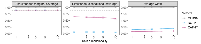
Figure 6: Performance on simulated heterogeneous trajectories of prediction bands constructed by different methods, as a function of the data dimensionality. See Table 3 for more detailed results and standard errors.

Table 3: Performance on simulated heterogeneous trajectories of prediction bands constructed by different methods, as a function of the data dimensionality. The red numbers indicate smaller prediction bands or higher conditional coverage. See the corresponding plot in Figure 6.

			Simultaneous coverage
Data dimensionality	Method	Average width	Conditional-hard	Conditional-easy	Marginal
1
1	CFRNN	2.000 (0.000)	0.995 (0.001)	1.000 (0.000)	1.000 (0.000)
1	NCTP	0.308 (0.014)	0.060 (0.008)	0.996 (0.001)	0.903 (0.002)
1	CAFHT	0.163 (0.001)	0.656 (0.010)	0.926 (0.002)	0.899 (0.003)
2
2	CFRNN	2.000 (0.000)	0.993 (0.001)	1.000 (0.000)	0.999 (0.000)
2	NCTP	0.338 (0.015)	0.064 (0.008)	0.996 (0.001)	0.905 (0.002)
2	CAFHT	0.172 (0.001)	0.630 (0.009)	0.930 (0.002)	0.901 (0.002)
3
3	CFRNN	2.000 (0.000)	0.993 (0.002)	1.000 (0.000)	0.999 (0.000)
3	NCTP	0.349 (0.016)	0.063 (0.008)	0.996 (0.001)	0.904 (0.002)
3	CAFHT	0.179 (0.001)	0.624 (0.012)	0.930 (0.002)	0.900 (0.002)
5
5	CFRNN	2.000 (0.000)	0.995 (0.001)	1.000 (0.000)	1.000 (0.000)
5	NCTP	0.378 (0.017)	0.066 (0.008)	0.996 (0.001)	0.904 (0.002)
5	CAFHT	0.188 (0.001)	0.619 (0.015)	0.931 (0.002)	0.900 (0.002)
10
10	CFRNN	2.000 (0.000)	0.993 (0.001)	1.000 (0.000)	0.999 (0.000)
10	NCTP	0.410 (0.020)	0.057 (0.008)	0.996 (0.001)	0.903 (0.002)
10	CAFHT	0.199 (0.001)	0.580 (0.013)	0.936 (0.002)	0.901 (0.003)

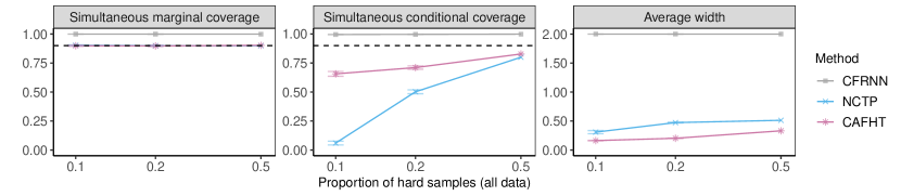
Figure 7: Performance on simulated heterogeneous trajectories of prediction bands constructed by different methods, as a function of the proportion of hard-to-predict trajectories. See Table 4 for more detailed results and standard errors.

Table 4: Performance on simulated heterogeneous trajectories of prediction bands constructed by different methods, as a function of the proportion of hard-to-predict trajectories. The red numbers indicate smaller prediction bands or higher conditional coverage. See the corresponding plot in Figure 7.

			Simultaneous coverage
Proportion of hard samples (all data)	Method	Average width	Conditional-hard	Conditional-easy	Marginal
0.1
0.1	CFRNN	2.000 (0.000)	0.995 (0.001)	1.000 (0.000)	1.000 (0.000)
0.1	NCTP	0.308 (0.014)	0.060 (0.008)	0.996 (0.001)	0.903 (0.002)
0.1	CAFHT	0.163 (0.001)	0.656 (0.010)	0.926 (0.002)	0.899 (0.003)
0.2
0.2	CFRNN	2.000 (0.000)	0.997 (0.001)	1.000 (0.000)	0.999 (0.000)
0.2	NCTP	0.473 (0.004)	0.502 (0.008)	1.000 (0.000)	0.900 (0.002)
0.2	CAFHT	0.203 (0.001)	0.710 (0.007)	0.944 (0.002)	0.897 (0.003)
0.5
0.5	CFRNN	2.000 (0.000)	0.999 (0.000)	1.000 (0.000)	0.999 (0.000)
0.5	NCTP	0.512 (0.004)	0.799 (0.004)	1.000 (0.000)	0.899 (0.002)
0.5	CAFHT	0.331 (0.002)	0.827 (0.005)	0.978 (0.001)	0.903 (0.003)

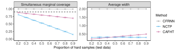
Figure 8: Performance on simulated heterogeneous trajectories of prediction bands constructed by different methods under distributional shift. The results are shown as a function of the proportion of hard-to-predict trajectories in the test data. See Table 5 for more detailed results and standard errors.

Table 5: Performance on simulated heterogeneous trajectories of prediction bands constructed by different methods under distributional shift. The results are shown as a function of the proportion of hard-to-predict trajectories in the test data. The red numbers indicate higher marginal coverage. See the corresponding plot in Figure 8.

Proportion of hard samples (test data)	Method	Length	Marginal coverage
0.2
0.2	CFRNN	2.000 (0.000)	0.999 (0.000)
0.2	NCTP	0.300 (0.016)	0.808 (0.003)
0.2	CAFHT	0.207 (0.002)	0.877 (0.003)
0.3
0.3	CFRNN	2.000 (0.000)	0.998 (0.000)
0.3	NCTP	0.315 (0.017)	0.716 (0.004)
0.3	CAFHT	0.250 (0.002)	0.849 (0.004)
0.4
0.4	CFRNN	2.000 (0.000)	0.997 (0.000)
0.4	NCTP	0.315 (0.016)	0.622 (0.004)
0.4	CAFHT	0.291 (0.003)	0.824 (0.004)
0.5
0.5	CFRNN	2.000 (0.000)	0.996 (0.000)
0.5	NCTP	0.316 (0.016)	0.530 (0.005)
0.5	CAFHT	0.334 (0.003)	0.795 (0.004)
0.6
0.6	CFRNN	2.000 (0.000)	0.996 (0.001)
0.6	NCTP	0.321 (0.016)	0.436 (0.006)
0.6	CAFHT	0.378 (0.003)	0.772 (0.004)
0.7
0.7	CFRNN	2.000 (0.000)	0.994 (0.001)
0.7	NCTP	0.310 (0.016)	0.341 (0.006)
0.7	CAFHT	0.422 (0.003)	0.743 (0.005)
0.8
0.8	CFRNN	2.000 (0.000)	0.994 (0.001)
0.8	NCTP	0.306 (0.017)	0.249 (0.008)
0.8	CAFHT	0.457 (0.004)	0.715 (0.005)
0.9
0.9	CFRNN	2.000 (0.000)	0.994 (0.001)
0.9	NCTP	0.301 (0.016)	0.152 (0.007)
0.9	CAFHT	0.500 (0.004)	0.692 (0.006)

AR data with static noise profile. Next, we present the results based on data generated from the AR model with the static noise profile.

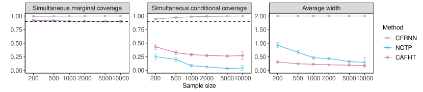
Figure 9: Performance on simulated heterogeneous trajectories of prediction bands constructed by different methods, as a function of the total number of training and calibration trajectories. See Table 6 for more detailed results and standard errors.

Table 6: Performance on simulated heterogeneous trajectories of prediction bands constructed by different methods, as a function of the total number of training and calibration trajectories. The red numbers indicate smaller prediction bands or higher conditional coverage. See the corresponding plot in Figure 9.

			Simultaneous coverage
Sample size	Method	Average width	Conditional-hard	Conditional-easy	Marginal
200
200	CFRNN	2.000 (0.000)	0.945 (0.006)	1.000 (0.000)	0.994 (0.001)
200	NCTP	0.927 (0.048)	0.251 (0.024)	0.990 (0.002)	0.916 (0.004)
200	CAFHT	0.311 (0.010)	0.434 (0.025)	0.968 (0.005)	0.914 (0.006)
500
500	CFRNN	2.000 (0.000)	0.972 (0.004)	1.000 (0.000)	0.997 (0.000)
500	NCTP	0.666 (0.031)	0.200 (0.020)	0.995 (0.002)	0.917 (0.003)
500	CAFHT	0.243 (0.005)	0.326 (0.017)	0.974 (0.003)	0.910 (0.004)
1000
1000	CFRNN	2.000 (0.000)	0.986 (0.002)	1.000 (0.000)	0.999 (0.000)
1000	NCTP	0.466 (0.030)	0.084 (0.011)	0.994 (0.001)	0.902 (0.002)
1000	CAFHT	0.227 (0.003)	0.289 (0.012)	0.976 (0.002)	0.906 (0.003)
2000
2000	CFRNN	2.000 (0.000)	0.993 (0.001)	1.000 (0.000)	0.999 (0.000)
2000	NCTP	0.435 (0.024)	0.063 (0.008)	0.996 (0.001)	0.904 (0.002)
2000	CAFHT	0.204 (0.002)	0.273 (0.008)	0.973 (0.002)	0.904 (0.002)
5000
5000	CFRNN	2.000 (0.000)	0.997 (0.001)	1.000 (0.000)	1.000 (0.000)
5000	NCTP	0.322 (0.024)	0.034 (0.006)	0.996 (0.001)	0.901 (0.002)
5000	CAFHT	0.194 (0.002)	0.263 (0.008)	0.973 (0.001)	0.902 (0.002)
10000
10000	CFRNN	2.000 (0.000)	1.000 (0.000)	1.000 (0.000)	1.000 (0.000)
10000	NCTP	0.299 (0.089)	0.044 (0.023)	0.997 (0.002)	0.907 (0.005)
10000	CAFHT	0.180 (0.005)	0.270 (0.037)	0.966 (0.004)	0.901 (0.006)

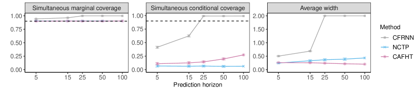
Figure 10: Performance on simulated heterogeneous trajectories of prediction bands constructed by different methods, as a function of the prediction horizon. See Table 7 for more detailed results and standard errors.

Table 7: Performance on simulated heterogeneous trajectories of prediction bands constructed by different methods, as a function of the prediction horizon. The red numbers indicate smaller prediction bands or higher conditional coverage. See corresponding plot in Figure 10.

			Simultaneous coverage
Prediction horizon	Method	Average width	Conditional-hard	Conditional-easy	Marginal
5
5	CFRNN	0.504 (0.009)	0.414 (0.010)	1.000 (0.000)	0.942 (0.001)
5	NCTP	0.246 (0.012)	0.067 (0.009)	0.996 (0.001)	0.904 (0.002)
5	CAFHT	0.260 (0.006)	0.110 (0.011)	0.987 (0.001)	0.901 (0.002)
15
15	CFRNN	0.688 (0.008)	0.624 (0.010)	1.000 (0.000)	0.963 (0.001)
15	NCTP	0.331 (0.018)	0.064 (0.008)	0.996 (0.001)	0.904 (0.002)
15	CAFHT	0.256 (0.004)	0.125 (0.011)	0.987 (0.001)	0.902 (0.002)
25
25	CFRNN	2.000 (0.000)	0.992 (0.002)	1.000 (0.000)	0.999 (0.000)
25	NCTP	0.368 (0.020)	0.067 (0.009)	0.996 (0.001)	0.905 (0.002)
25	CAFHT	0.241 (0.003)	0.144 (0.008)	0.984 (0.001)	0.902 (0.002)
50
50	CFRNN	2.000 (0.000)	0.992 (0.002)	1.000 (0.000)	0.999 (0.000)
50	NCTP	0.390 (0.023)	0.061 (0.008)	0.996 (0.001)	0.904 (0.002)
50	CAFHT	0.218 (0.002)	0.198 (0.010)	0.978 (0.002)	0.901 (0.002)
100
100	CFRNN	2.000 (0.000)	0.993 (0.001)	1.000 (0.000)	0.999 (0.000)
100	NCTP	0.435 (0.024)	0.063 (0.008)	0.996 (0.001)	0.904 (0.002)
100	CAFHT	0.204 (0.002)	0.273 (0.008)	0.973 (0.002)	0.904 (0.002)

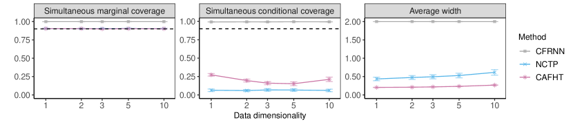
Figure 11: Performance on simulated heterogeneous trajectories of prediction bands constructed by different methods, as a function of the data dimensionality. See Table 8 for more detailed results and standard errors.

Table 8: Performance on simulated heterogeneous trajectories of prediction bands constructed by different methods, as a function of the data dimensionality. The red numbers indicate smaller prediction bands or higher conditional coverage. See the corresponding plot in Figure 11.

			Simultaneous coverage
Data dimensionality	Method	Average width	Conditional-hard	Conditional-easy	Marginal
1
1	CFRNN	2.000 (0.000)	0.993 (0.001)	1.000 (0.000)	0.999 (0.000)
1	NCTP	0.435 (0.024)	0.063 (0.008)	0.996 (0.001)	0.904 (0.002)
1	CAFHT	0.204 (0.002)	0.273 (0.008)	0.973 (0.002)	0.904 (0.002)
2
2	CFRNN	2.000 (0.000)	0.994 (0.001)	1.000 (0.000)	0.999 (0.000)
2	NCTP	0.475 (0.027)	0.059 (0.007)	0.996 (0.001)	0.903 (0.002)
2	CAFHT	0.210 (0.002)	0.195 (0.009)	0.981 (0.001)	0.904 (0.002)
3
3	CFRNN	2.000 (0.000)	0.993 (0.001)	1.000 (0.000)	0.999 (0.000)
3	NCTP	0.495 (0.028)	0.068 (0.009)	0.996 (0.001)	0.904 (0.002)
3	CAFHT	0.219 (0.003)	0.160 (0.011)	0.982 (0.001)	0.900 (0.002)
5
5	CFRNN	2.000 (0.000)	0.995 (0.001)	1.000 (0.000)	1.000 (0.000)
5	NCTP	0.529 (0.032)	0.066 (0.009)	0.997 (0.001)	0.906 (0.002)
5	CAFHT	0.234 (0.003)	0.152 (0.013)	0.985 (0.002)	0.903 (0.002)
10
10	CFRNN	2.000 (0.000)	0.994 (0.001)	1.000 (0.000)	0.999 (0.000)
10	NCTP	0.615 (0.038)	0.061 (0.008)	0.997 (0.001)	0.904 (0.002)
10	CAFHT	0.267 (0.003)	0.212 (0.015)	0.978 (0.002)	0.902 (0.003)

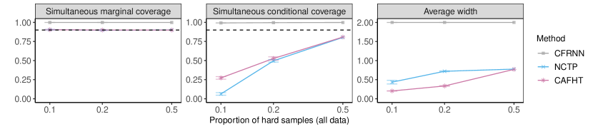
Figure 12: Performance on simulated heterogeneous trajectories of prediction bands constructed by different methods, as a function of the proportion of hard-to-predict trajectories. See Table 9 for more detailed results and standard errors.

Table 9: Performance on simulated heterogeneous trajectories of prediction bands constructed by different methods, as a function of the proportion of hard-to-predict trajectories. The red numbers indicate smaller prediction bands or higher conditional coverage. See the corresponding plot in Figure 12.

			Simultaneous coverage
Proportion of hard samples (all data)	Method	Average width	Conditional-hard	Conditional-easy	Marginal
0.1
0.1	CFRNN	2.000 (0.000)	0.993 (0.001)	1.000 (0.000)	0.999 (0.000)
0.1	NCTP	0.435 (0.024)	0.063 (0.008)	0.996 (0.001)	0.904 (0.002)
0.1	CAFHT	0.204 (0.002)	0.273 (0.008)	0.973 (0.002)	0.904 (0.002)
0.2
0.2	CFRNN	2.000 (0.000)	0.996 (0.001)	1.000 (0.000)	0.999 (0.000)
0.2	NCTP	0.720 (0.006)	0.496 (0.008)	1.000 (0.000)	0.898 (0.002)
0.2	CAFHT	0.335 (0.005)	0.527 (0.011)	0.993 (0.001)	0.900 (0.003)
0.5
0.5	CFRNN	2.000 (0.000)	0.999 (0.000)	1.000 (0.000)	0.999 (0.000)
0.5	NCTP	0.776 (0.005)	0.803 (0.003)	1.000 (0.000)	0.901 (0.002)
0.5	CAFHT	0.770 (0.007)	0.808 (0.004)	0.992 (0.001)	0.900 (0.002)

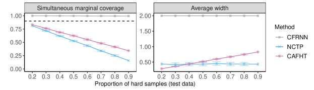
Figure 13: Performance on simulated heterogeneous trajectories of prediction bands constructed by different methods under distributional shift. The results are shown as a function of the proportion of hard-to-predict trajectories in the test data. See Table 10 for detailed results and standard errors.

Table 10: Performance on simulated heterogeneous trajectories of prediction bands constructed by different methods under distributional shift. The results are shown as a function of the proportion of hard-to-predict trajectories in the test data. The red numbers indicate higher marginal coverage. See the corresponding plot in Figure 13.

Proportion of hard samples (test data)	Method	Length	Marginal coverage
0.2
0.2	CFRNN	2.000 (0.000)	0.999 (0.000)
0.2	NCTP	0.437 (0.028)	0.811 (0.003)
0.2	CAFHT	0.284 (0.003)	0.832 (0.003)
0.3
0.3	CFRNN	2.000 (0.000)	0.998 (0.000)
0.3	NCTP	0.419 (0.027)	0.715 (0.004)
0.3	CAFHT	0.359 (0.004)	0.762 (0.004)
0.4
0.4	CFRNN	2.000 (0.000)	0.998 (0.000)
0.4	NCTP	0.432 (0.026)	0.619 (0.004)
0.4	CAFHT	0.438 (0.005)	0.689 (0.004)
0.5
0.5	CFRNN	2.000 (0.000)	0.997 (0.000)
0.5	NCTP	0.431 (0.027)	0.526 (0.005)
0.5	CAFHT	0.517 (0.006)	0.624 (0.005)
0.6
0.6	CFRNN	2.000 (0.000)	0.996 (0.001)
0.6	NCTP	0.451 (0.028)	0.438 (0.006)
0.6	CAFHT	0.598 (0.007)	0.552 (0.005)
0.7
0.7	CFRNN	2.000 (0.000)	0.996 (0.001)
0.7	NCTP	0.436 (0.027)	0.340 (0.006)
0.7	CAFHT	0.671 (0.008)	0.481 (0.006)
0.8
0.8	CFRNN	2.000 (0.000)	0.996 (0.001)
0.8	NCTP	0.437 (0.027)	0.252 (0.007)
0.8	CAFHT	0.746 (0.009)	0.414 (0.006)
0.9
0.9	CFRNN	2.000 (0.000)	0.995 (0.001)
0.9	NCTP	0.432 (0.027)	0.157 (0.007)
0.9	CAFHT	0.828 (0.010)	0.343 (0.007)

E.1.2 Supplementary Results — Comparing Different Versions of CAFHT

In this subsection, we add different versions of CAFHT into comparison. We will separately analyze the CAFHT prediction bands constructed using multiplicative conformity scores (6) and those constructed using additive conformity scores (3). The conclusions from the results evaluated using synthetic data with the dynamic profile and with the static profile are very similar. To save space, we only demonstrate the results using data with the static profile.

We consider the following CAFHT methods:

• CAFHT: the main method. It is the CAFHT method based on the ACI prediction band using the data splitting strategy; see Algorithm 3

• CAFHT - PID: the CAFHT method based on the PID prediction band using the data splitting strategy. It can be implemented simply by substituting $\hat{C}^{\text{ACI}}$ to $\hat{C}^{\text{PID}}$ in Algorithm 3 wherever possible.

• CAFHT (theory): the CAFHT method based on the ACI prediction band after correcting the theoretical coverage; see Appendix D and Algorithm 7.

• CAFHT (theory) - PID: the CAFHT method based on the PID prediction band after correcting the theoretical coverage. It can be implemented simply by substituting $\hat{C}^{\text{ACI}}$ to $\hat{C}^{\text{PID}}$ in Algorithm 7 wherever possible.

CAFHT — Multiplicative Scores

The results of CAFHT methods with multiplicative conformity scores (6) are first presented.

Similar to what we have observed from the results in subsection E.1.1, the CAFHT methods outperform the benchmark methods (CFRNN and NCTP) across all configurations we considered. Generally, CAFHT methods produce narrower, more informative bands with higher conditional coverage. Among the different versions of CAFHT, the prediction bands generated using the theoretical correction approach (outlined in D) tend to be more conservative compared to those from the data-splitting approach. Additionally, in our experiments, the performance of prediction bands constructed by CAFHT with ACI is empirically similar to those created using PID.

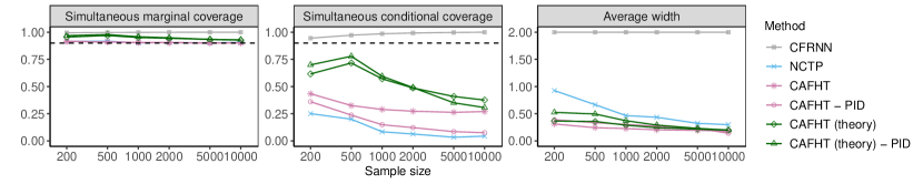
Figure 14: Performance on simulated heterogeneous trajectories of prediction bands constructed by different methods, as a function of the total number of training and calibration trajectories. See Table 11 for detailed results and standard errors.

Table 11: Performance on simulated heterogeneous trajectories of prediction bands constructed by different methods, as a function of the total number of training and calibration trajectories. The red numbers indicate smaller prediction bands or higher conditional coverage. See corresponding plot in Figure 14.

			Simultaneous coverage
Sample size	Method	Average width	Conditional-hard	Conditional-easy	Marginal
200
200	CFRNN	2.000 (0.000)	0.945 (0.006)	1.000 (0.000)	0.994 (0.001)
200	NCTP	0.927 (0.048)	0.251 (0.024)	0.990 (0.002)	0.916 (0.004)
200	CAFHT	0.311 (0.010)	0.434 (0.025)	0.968 (0.005)	0.914 (0.006)
200	CAFHT - PID	0.390 (0.022)	0.361 (0.027)	0.978 (0.004)	0.916 (0.006)
200	CAFHT (theory)	0.365 (0.009)	0.616 (0.016)	0.993 (0.001)	0.955 (0.002)
200	CAFHT (theory) - PID	0.525 (0.014)	0.700 (0.018)	0.998 (0.001)	0.968 (0.002)
500
500	CFRNN	2.000 (0.000)	0.972 (0.004)	1.000 (0.000)	0.997 (0.000)
500	NCTP	0.666 (0.031)	0.200 (0.020)	0.995 (0.002)	0.917 (0.003)
500	CAFHT	0.243 (0.005)	0.326 (0.017)	0.974 (0.003)	0.910 (0.004)
500	CAFHT - PID	0.335 (0.021)	0.237 (0.022)	0.983 (0.003)	0.910 (0.004)
500	CAFHT (theory)	0.358 (0.006)	0.717 (0.012)	0.997 (0.001)	0.970 (0.001)
500	CAFHT (theory) - PID	0.495 (0.009)	0.779 (0.013)	1.000 (0.000)	0.978 (0.001)
1000
1000	CFRNN	2.000 (0.000)	0.986 (0.002)	1.000 (0.000)	0.999 (0.000)
1000	NCTP	0.466 (0.030)	0.084 (0.011)	0.994 (0.001)	0.902 (0.002)
1000	CAFHT	0.227 (0.003)	0.289 (0.012)	0.976 (0.002)	0.906 (0.003)
1000	CAFHT - PID	0.303 (0.018)	0.149 (0.014)	0.988 (0.002)	0.903 (0.003)
1000	CAFHT (theory)	0.290 (0.004)	0.571 (0.013)	0.994 (0.001)	0.951 (0.002)
1000	CAFHT (theory) - PID	0.371 (0.007)	0.595 (0.014)	0.999 (0.000)	0.958 (0.002)
2000
2000	CFRNN	2.000 (0.000)	0.993 (0.001)	1.000 (0.000)	0.999 (0.000)
2000	NCTP	0.435 (0.024)	0.063 (0.008)	0.996 (0.001)	0.904 (0.002)
2000	CAFHT	0.204 (0.002)	0.273 (0.008)	0.973 (0.002)	0.904 (0.002)
2000	CAFHT - PID	0.270 (0.016)	0.122 (0.012)	0.989 (0.001)	0.904 (0.002)
2000	CAFHT (theory)	0.243 (0.003)	0.487 (0.010)	0.994 (0.001)	0.944 (0.001)
2000	CAFHT (theory) - PID	0.291 (0.004)	0.490 (0.011)	0.999 (0.000)	0.949 (0.002)
5000
5000	CFRNN	2.000 (0.000)	0.997 (0.001)	1.000 (0.000)	1.000 (0.000)
5000	NCTP	0.322 (0.024)	0.034 (0.006)	0.996 (0.001)	0.901 (0.002)
5000	CAFHT	0.194 (0.002)	0.263 (0.008)	0.973 (0.001)	0.902 (0.002)
5000	CAFHT - PID	0.233 (0.015)	0.085 (0.009)	0.990 (0.001)	0.900 (0.002)
5000	CAFHT (theory)	0.217 (0.002)	0.409 (0.008)	0.991 (0.001)	0.933 (0.001)
5000	CAFHT (theory) - PID	0.231 (0.003)	0.351 (0.010)	0.998 (0.000)	0.934 (0.001)
10000
10000	CFRNN	2.000 (0.000)	1.000 (0.000)	1.000 (0.000)	1.000 (0.000)
10000	NCTP	0.299 (0.089)	0.044 (0.023)	0.997 (0.002)	0.907 (0.005)
10000	CAFHT	0.180 (0.005)	0.270 (0.037)	0.966 (0.004)	0.901 (0.006)
10000	CAFHT - PID	0.140 (0.016)	0.076 (0.039)	0.989 (0.004)	0.903 (0.005)
10000	CAFHT (theory)	0.196 (0.005)	0.376 (0.033)	0.985 (0.002)	0.927 (0.006)
10000	CAFHT (theory) - PID	0.200 (0.008)	0.307 (0.045)	0.994 (0.001)	0.930 (0.004)

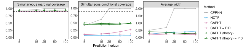
Figure 15: Performance on simulated heterogeneous trajectories of prediction bands constructed by different methods, as a function of the prediction horizon. See Table 12 for detailed results and standard errors.

Table 12: Performance on simulated heterogeneous trajectories of prediction bands constructed by different methods, as a function of the prediction horizon. The red numbers indicate smaller prediction bands or higher conditional coverage. See the corresponding plot in Figure 15.

			Simultaneous coverage
Prediction horizon	Method	Average width	Conditional-hard	Conditional-easy	Marginal
5
5	CFRNN	0.504 (0.009)	0.414 (0.010)	1.000 (0.000)	0.942 (0.001)
5	NCTP	0.246 (0.012)	0.067 (0.009)	0.996 (0.001)	0.904 (0.002)
5	CAFHT	0.260 (0.006)	0.110 (0.011)	0.987 (0.001)	0.901 (0.002)
5	CAFHT - PID	0.190 (0.008)	0.098 (0.011)	0.991 (0.001)	0.903 (0.002)
5	CAFHT (theory)	0.406 (0.007)	0.444 (0.012)	0.998 (0.000)	0.944 (0.002)
5	CAFHT (theory) - PID	0.309 (0.005)	0.503 (0.014)	0.996 (0.001)	0.947 (0.002)
15
15	CFRNN	0.688 (0.008)	0.624 (0.010)	1.000 (0.000)	0.963 (0.001)
15	NCTP	0.331 (0.018)	0.064 (0.008)	0.996 (0.001)	0.904 (0.002)
15	CAFHT	0.256 (0.004)	0.125 (0.011)	0.987 (0.001)	0.902 (0.002)
15	CAFHT - PID	0.235 (0.014)	0.125 (0.012)	0.987 (0.002)	0.902 (0.003)
15	CAFHT (theory)	0.359 (0.005)	0.442 (0.012)	0.998 (0.000)	0.944 (0.001)
15	CAFHT (theory) - PID	0.304 (0.006)	0.483 (0.012)	0.999 (0.000)	0.948 (0.002)
25
25	CFRNN	2.000 (0.000)	0.992 (0.002)	1.000 (0.000)	0.999 (0.000)
25	NCTP	0.368 (0.020)	0.067 (0.009)	0.996 (0.001)	0.905 (0.002)
25	CAFHT	0.241 (0.003)	0.144 (0.008)	0.984 (0.001)	0.902 (0.002)
25	CAFHT - PID	0.247 (0.015)	0.129 (0.013)	0.987 (0.002)	0.903 (0.003)
25	CAFHT (theory)	0.321 (0.004)	0.442 (0.012)	0.998 (0.000)	0.944 (0.002)
25	CAFHT (theory) - PID	0.302 (0.005)	0.487 (0.011)	0.999 (0.000)	0.949 (0.001)
50
50	CFRNN	2.000 (0.000)	0.992 (0.002)	1.000 (0.000)	0.999 (0.000)
50	NCTP	0.390 (0.023)	0.061 (0.008)	0.996 (0.001)	0.904 (0.002)
50	CAFHT	0.218 (0.002)	0.198 (0.010)	0.978 (0.002)	0.901 (0.002)
50	CAFHT - PID	0.260 (0.017)	0.117 (0.014)	0.991 (0.001)	0.905 (0.003)
50	CAFHT (theory)	0.274 (0.003)	0.456 (0.011)	0.996 (0.000)	0.943 (0.002)
50	CAFHT (theory) - PID	0.296 (0.005)	0.494 (0.011)	0.998 (0.000)	0.949 (0.002)
100
100	CFRNN	2.000 (0.000)	0.993 (0.001)	1.000 (0.000)	0.999 (0.000)
100	NCTP	0.435 (0.024)	0.063 (0.008)	0.996 (0.001)	0.904 (0.002)
100	CAFHT	0.204 (0.002)	0.273 (0.008)	0.973 (0.002)	0.904 (0.002)
100	CAFHT - PID	0.270 (0.016)	0.122 (0.012)	0.989 (0.001)	0.904 (0.002)
100	CAFHT (theory)	0.243 (0.003)	0.487 (0.010)	0.994 (0.001)	0.944 (0.001)
100	CAFHT (theory) - PID	0.291 (0.004)	0.490 (0.011)	0.999 (0.000)	0.949 (0.002)

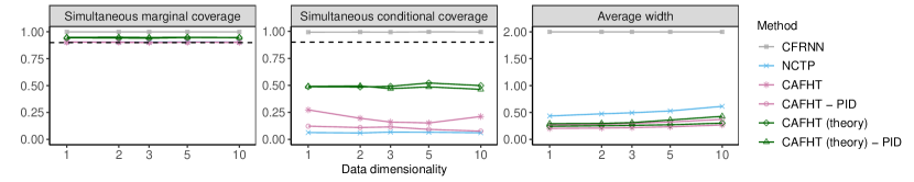
Figure 16: Performance on simulated heterogeneous trajectories of prediction bands constructed by different methods, as a function of the data dimensionality. See Table 13 for detailed results and standard errors.

Table 13: Performance on simulated heterogeneous trajectories of prediction bands constructed by different methods, as a function of the data dimensionality. The red numbers indicate smaller prediction bands or higher conditional coverage. See the corresponding plot in Figure 16.

			Simultaneous coverage
Data dimensionality	Method	Average width	Conditional-hard	Conditional-easy	Marginal
1
1	CFRNN	2.000 (0.000)	0.993 (0.001)	1.000 (0.000)	0.999 (0.000)
1	NCTP	0.435 (0.024)	0.063 (0.008)	0.996 (0.001)	0.904 (0.002)
1	CAFHT	0.204 (0.002)	0.273 (0.008)	0.973 (0.002)	0.904 (0.002)
1	CAFHT - PID	0.270 (0.016)	0.122 (0.012)	0.989 (0.001)	0.904 (0.002)
1	CAFHT (theory)	0.243 (0.003)	0.487 (0.010)	0.994 (0.001)	0.944 (0.001)
1	CAFHT (theory) - PID	0.291 (0.004)	0.490 (0.011)	0.999 (0.000)	0.949 (0.002)
2
2	CFRNN	2.000 (0.000)	0.994 (0.001)	1.000 (0.000)	0.999 (0.000)
2	NCTP	0.475 (0.027)	0.059 (0.007)	0.996 (0.001)	0.903 (0.002)
2	CAFHT	0.210 (0.002)	0.195 (0.009)	0.981 (0.001)	0.904 (0.002)
2	CAFHT - PID	0.283 (0.017)	0.110 (0.010)	0.988 (0.001)	0.902 (0.002)
2	CAFHT (theory)	0.253 (0.002)	0.485 (0.012)	0.993 (0.001)	0.943 (0.001)
2	CAFHT (theory) - PID	0.297 (0.004)	0.495 (0.012)	0.999 (0.000)	0.949 (0.001)
3
3	CFRNN	2.000 (0.000)	0.993 (0.001)	1.000 (0.000)	0.999 (0.000)
3	NCTP	0.495 (0.028)	0.068 (0.009)	0.996 (0.001)	0.904 (0.002)
3	CAFHT	0.219 (0.003)	0.160 (0.011)	0.982 (0.001)	0.900 (0.002)
3	CAFHT - PID	0.297 (0.018)	0.115 (0.012)	0.988 (0.001)	0.902 (0.002)
3	CAFHT (theory)	0.260 (0.003)	0.491 (0.012)	0.990 (0.001)	0.941 (0.001)
3	CAFHT (theory) - PID	0.312 (0.004)	0.470 (0.011)	1.000 (0.000)	0.947 (0.001)
5
5	CFRNN	2.000 (0.000)	0.995 (0.001)	1.000 (0.000)	1.000 (0.000)
5	NCTP	0.529 (0.032)	0.066 (0.009)	0.997 (0.001)	0.906 (0.002)
5	CAFHT	0.234 (0.003)	0.152 (0.013)	0.985 (0.002)	0.903 (0.002)
5	CAFHT - PID	0.323 (0.021)	0.093 (0.010)	0.991 (0.001)	0.903 (0.002)
5	CAFHT (theory)	0.271 (0.003)	0.522 (0.011)	0.992 (0.001)	0.946 (0.002)
5	CAFHT (theory) - PID	0.360 (0.004)	0.486 (0.012)	1.000 (0.000)	0.949 (0.002)
10
10	CFRNN	2.000 (0.000)	0.994 (0.001)	1.000 (0.000)	0.999 (0.000)
10	NCTP	0.615 (0.038)	0.061 (0.008)	0.997 (0.001)	0.904 (0.002)
10	CAFHT	0.267 (0.003)	0.212 (0.015)	0.978 (0.002)	0.902 (0.003)
10	CAFHT - PID	0.372 (0.023)	0.076 (0.011)	0.993 (0.001)	0.902 (0.002)
10	CAFHT (theory)	0.303 (0.003)	0.498 (0.009)	0.995 (0.001)	0.946 (0.001)
10	CAFHT (theory) - PID	0.428 (0.003)	0.463 (0.012)	1.000 (0.000)	0.947 (0.001)

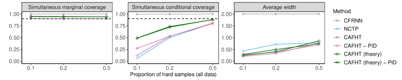
Figure 17: Performance on simulated heterogeneous trajectories of prediction bands constructed by different methods, as a function of the proportion of hard-to-predict trajectories. See Table 14 for detailed results and standard errors.

Table 14: Performance on simulated heterogeneous trajectories of prediction bands constructed by different methods, as a function of the proportion of hard-to-predict trajectories. The red numbers indicate smaller prediction bands or higher conditional coverage. See the corresponding plot in Figure 17.

			Simultaneous coverage
Proportion of hard samples (all data)	Method	Average width	Conditional-hard	Conditional-easy	Marginal
0.1
0.1	CFRNN	2.000 (0.000)	0.993 (0.001)	1.000 (0.000)	0.999 (0.000)
0.1	NCTP	0.435 (0.024)	0.063 (0.008)	0.996 (0.001)	0.904 (0.002)
0.1	CAFHT	0.204 (0.002)	0.273 (0.008)	0.973 (0.002)	0.904 (0.002)
0.1	CAFHT - PID	0.270 (0.016)	0.122 (0.012)	0.989 (0.001)	0.904 (0.002)
0.1	CAFHT (theory)	0.243 (0.003)	0.487 (0.010)	0.994 (0.001)	0.944 (0.001)
0.1	CAFHT (theory) - PID	0.291 (0.004)	0.490 (0.011)	0.999 (0.000)	0.949 (0.002)
0.2
0.2	CFRNN	2.000 (0.000)	0.996 (0.001)	1.000 (0.000)	0.999 (0.000)
0.2	NCTP	0.720 (0.006)	0.496 (0.008)	1.000 (0.000)	0.898 (0.002)
0.2	CAFHT	0.335 (0.005)	0.527 (0.011)	0.993 (0.001)	0.900 (0.003)
0.2	CAFHT - PID	0.388 (0.005)	0.528 (0.010)	0.993 (0.001)	0.899 (0.002)
0.2	CAFHT (theory)	0.404 (0.005)	0.721 (0.007)	0.996 (0.001)	0.940 (0.001)
0.2	CAFHT (theory) - PID	0.498 (0.005)	0.733 (0.007)	0.999 (0.000)	0.946 (0.001)
0.5
0.5	CFRNN	2.000 (0.000)	0.999 (0.000)	1.000 (0.000)	0.999 (0.000)
0.5	NCTP	0.776 (0.005)	0.803 (0.003)	1.000 (0.000)	0.901 (0.002)
0.5	CAFHT	0.770 (0.007)	0.808 (0.004)	0.992 (0.001)	0.900 (0.002)
0.5	CAFHT - PID	0.694 (0.005)	0.796 (0.004)	1.000 (0.000)	0.898 (0.002)
0.5	CAFHT (theory)	0.858 (0.007)	0.880 (0.003)	0.998 (0.000)	0.939 (0.001)
0.5	CAFHT (theory) - PID	0.741 (0.005)	0.878 (0.003)	1.000 (0.000)	0.939 (0.002)

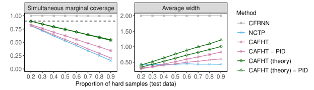
Figure 18: Performance on simulated heterogeneous trajectories of prediction bands constructed by different methods under distributional shift. The results are shown as a function of the proportion of hard-to-predict trajectories in the test data. See Table 15 for detailed results and standard errors.

Table 15: Performance on simulated heterogeneous trajectories of prediction bands constructed by different methods under distributional shift. The results are shown as a function of the proportion of hard-to-predict trajectories in the test data. The red numbers indicate higher marginal coverage. See the corresponding plot in Figure 18.

Proportion of hard samples (test data)	Method	Length	Marginal coverage
0.2
0.2	CFRNN	2.000 (0.000)	0.999 (0.000)
0.2	NCTP	0.437 (0.028)	0.811 (0.003)
0.2	CAFHT	0.284 (0.003)	0.832 (0.003)
0.2	CAFHT - PID	0.316 (0.018)	0.816 (0.003)
0.2	CAFHT (theory)	0.342 (0.005)	0.896 (0.002)
0.2	CAFHT (theory) - PID	0.411 (0.008)	0.896 (0.003)
0.3
0.3	CFRNN	2.000 (0.000)	0.998 (0.000)
0.3	NCTP	0.419 (0.027)	0.715 (0.004)
0.3	CAFHT	0.359 (0.004)	0.762 (0.004)
0.3	CAFHT - PID	0.353 (0.017)	0.728 (0.004)
0.3	CAFHT (theory)	0.434 (0.006)	0.844 (0.003)
0.3	CAFHT (theory) - PID	0.521 (0.010)	0.842 (0.003)
0.4
0.4	CFRNN	2.000 (0.000)	0.998 (0.000)
0.4	NCTP	0.432 (0.026)	0.619 (0.004)
0.4	CAFHT	0.438 (0.005)	0.689 (0.004)
0.4	CAFHT - PID	0.402 (0.017)	0.640 (0.005)
0.4	CAFHT (theory)	0.532 (0.007)	0.794 (0.003)
0.4	CAFHT (theory) - PID	0.639 (0.011)	0.788 (0.004)
0.5
0.5	CFRNN	2.000 (0.000)	0.997 (0.000)
0.5	NCTP	0.431 (0.027)	0.526 (0.005)
0.5	CAFHT	0.517 (0.006)	0.624 (0.005)
0.5	CAFHT - PID	0.448 (0.017)	0.552 (0.006)
0.5	CAFHT (theory)	0.628 (0.009)	0.746 (0.004)
0.5	CAFHT (theory) - PID	0.764 (0.013)	0.743 (0.005)
0.6
0.6	CFRNN	2.000 (0.000)	0.996 (0.001)
0.6	NCTP	0.451 (0.028)	0.438 (0.006)
0.6	CAFHT	0.598 (0.007)	0.552 (0.005)
0.6	CAFHT - PID	0.499 (0.020)	0.469 (0.007)
0.6	CAFHT (theory)	0.730 (0.011)	0.696 (0.005)
0.6	CAFHT (theory) - PID	0.883 (0.016)	0.693 (0.006)
0.7
0.7	CFRNN	2.000 (0.000)	0.996 (0.001)
0.7	NCTP	0.436 (0.027)	0.340 (0.006)
0.7	CAFHT	0.671 (0.008)	0.481 (0.006)
0.7	CAFHT - PID	0.531 (0.022)	0.376 (0.008)
0.7	CAFHT (theory)	0.819 (0.012)	0.644 (0.005)
0.7	CAFHT (theory) - PID	0.996 (0.019)	0.640 (0.007)
0.8
0.8	CFRNN	2.000 (0.000)	0.996 (0.001)
0.8	NCTP	0.437 (0.027)	0.252 (0.007)
0.8	CAFHT	0.746 (0.009)	0.414 (0.006)
0.8	CAFHT - PID	0.574 (0.023)	0.292 (0.008)
0.8	CAFHT (theory)	0.911 (0.013)	0.597 (0.005)
0.8	CAFHT (theory) - PID	1.094 (0.020)	0.589 (0.008)
0.9
0.9	CFRNN	2.000 (0.000)	0.995 (0.001)
0.9	NCTP	0.432 (0.027)	0.157 (0.007)
0.9	CAFHT	0.828 (0.010)	0.343 (0.007)
0.9	CAFHT - PID	0.606 (0.027)	0.205 (0.010)
0.9	CAFHT (theory)	1.006 (0.014)	0.548 (0.006)
0.9	CAFHT (theory) - PID	1.218 (0.023)	0.537 (0.009)

CAFHT — Additive Scores

Finally, the results of CAFHT methods with additive conformity scores (3) are presented.

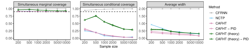
Figure 19: Performance on simulated heterogeneous trajectories of prediction bands constructed by different methods, as a function of the total number of training and calibration trajectories. See Table 16 for detailed results and standard errors.

Table 16: Performance on simulated heterogeneous trajectories of prediction bands constructed by different methods, as a function of the total number of training and calibration trajectories. The red numbers indicate smaller prediction bands or higher conditional coverage. See the corresponding plot in Figure 19.

			Simultaneous coverage
Sample size	Method	Average width	Conditional-hard	Conditional-easy	Marginal
200
200	CFRNN	2.000 (0.000)	0.945 (0.006)	1.000 (0.000)	0.994 (0.001)
200	NCTP	0.927 (0.048)	0.251 (0.024)	0.990 (0.002)	0.916 (0.004)
200	CAFHT	0.388 (0.018)	0.290 (0.030)	0.982 (0.004)	0.913 (0.006)
200	CAFHT - PID	0.466 (0.026)	0.326 (0.031)	0.980 (0.004)	0.915 (0.006)
200	CAFHT (theory)	0.576 (0.015)	0.621 (0.023)	1.000 (0.000)	0.963 (0.002)
200	CAFHT (theory) - PID	0.614 (0.016)	0.620 (0.024)	1.000 (0.000)	0.962 (0.002)
500
500	CFRNN	2.000 (0.000)	0.972 (0.004)	1.000 (0.000)	0.997 (0.000)
500	NCTP	0.666 (0.031)	0.200 (0.020)	0.995 (0.002)	0.917 (0.003)
500	CAFHT	0.323 (0.013)	0.195 (0.023)	0.988 (0.003)	0.911 (0.004)
500	CAFHT - PID	0.399 (0.024)	0.190 (0.022)	0.988 (0.003)	0.910 (0.004)
500	CAFHT (theory)	0.572 (0.008)	0.762 (0.016)	1.000 (0.000)	0.977 (0.002)
500	CAFHT (theory) - PID	0.600 (0.009)	0.753 (0.015)	1.000 (0.000)	0.976 (0.001)
1000
1000	CFRNN	2.000 (0.000)	0.986 (0.002)	1.000 (0.000)	0.999 (0.000)
1000	NCTP	0.466 (0.030)	0.084 (0.011)	0.994 (0.001)	0.902 (0.002)
1000	CAFHT	0.289 (0.010)	0.115 (0.015)	0.993 (0.001)	0.904 (0.003)
1000	CAFHT - PID	0.362 (0.021)	0.119 (0.015)	0.993 (0.001)	0.904 (0.003)
1000	CAFHT (theory)	0.460 (0.006)	0.557 (0.015)	1.000 (0.000)	0.955 (0.002)
1000	CAFHT (theory) - PID	0.481 (0.006)	0.559 (0.013)	1.000 (0.000)	0.955 (0.002)
2000
2000	CFRNN	2.000 (0.000)	0.993 (0.001)	1.000 (0.000)	0.999 (0.000)
2000	NCTP	0.435 (0.024)	0.063 (0.008)	0.996 (0.001)	0.904 (0.002)
2000	CAFHT	0.241 (0.008)	0.069 (0.010)	0.993 (0.001)	0.901 (0.002)
2000	CAFHT - PID	0.306 (0.019)	0.081 (0.012)	0.994 (0.001)	0.904 (0.002)
2000	CAFHT (theory)	0.393 (0.004)	0.434 (0.011)	1.000 (0.000)	0.944 (0.001)
2000	CAFHT (theory) - PID	0.407 (0.004)	0.452 (0.011)	1.000 (0.000)	0.946 (0.001)
5000
5000	CFRNN	2.000 (0.000)	0.997 (0.001)	1.000 (0.000)	1.000 (0.000)
5000	NCTP	0.322 (0.024)	0.034 (0.006)	0.996 (0.001)	0.901 (0.002)
5000	CAFHT	0.214 (0.007)	0.035 (0.006)	0.994 (0.001)	0.899 (0.002)
5000	CAFHT - PID	0.260 (0.017)	0.040 (0.006)	0.994 (0.001)	0.899 (0.002)
5000	CAFHT (theory)	0.348 (0.003)	0.308 (0.008)	1.000 (0.000)	0.931 (0.001)
5000	CAFHT (theory) - PID	0.354 (0.003)	0.313 (0.009)	1.000 (0.000)	0.932 (0.001)
10000
10000	CFRNN	2.000 (0.000)	1.000 (0.000)	1.000 (0.000)	1.000 (0.000)
10000	NCTP	0.299 (0.089)	0.044 (0.023)	0.997 (0.002)	0.907 (0.005)
10000	CAFHT	0.176 (0.023)	0.030 (0.025)	0.994 (0.002)	0.903 (0.004)
10000	CAFHT - PID	0.154 (0.026)	0.025 (0.023)	0.997 (0.001)	0.905 (0.005)
10000	CAFHT (theory)	0.315 (0.005)	0.296 (0.016)	1.000 (0.000)	0.933 (0.004)
10000	CAFHT (theory) - PID	0.319 (0.007)	0.284 (0.042)	1.000 (0.000)	0.932 (0.005)

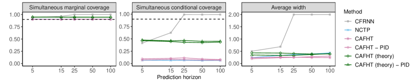
Figure 20: Performance on simulated heterogeneous trajectories of prediction bands constructed by different methods, as a function of the prediction horizon. See Table 17 for detailed results and standard errors.

Table 17: Performance on simulated heterogeneous trajectories of prediction bands constructed by different methods, as a function of the prediction horizon. The red numbers indicate smaller prediction bands or higher conditional coverage. See the corresponding plot in Figure 20.

			Simultaneous coverage
Prediction horizon	Method	Average width	Conditional-hard	Conditional-easy	Marginal
5
5	CFRNN	0.504 (0.009)	0.414 (0.010)	1.000 (0.000)	0.942 (0.001)
5	NCTP	0.246 (0.012)	0.067 (0.009)	0.996 (0.001)	0.904 (0.002)
5	CAFHT	0.237 (0.008)	0.073 (0.009)	0.993 (0.001)	0.902 (0.002)
5	CAFHT - PID	0.195 (0.008)	0.096 (0.010)	0.990 (0.001)	0.902 (0.002)
5	CAFHT (theory)	0.436 (0.008)	0.463 (0.012)	1.000 (0.000)	0.947 (0.002)
5	CAFHT (theory) - PID	0.348 (0.008)	0.477 (0.012)	1.000 (0.000)	0.948 (0.002)
15
15	CFRNN	0.688 (0.008)	0.624 (0.010)	1.000 (0.000)	0.963 (0.001)
15	NCTP	0.331 (0.018)	0.064 (0.008)	0.996 (0.001)	0.904 (0.002)
15	CAFHT	0.263 (0.008)	0.084 (0.010)	0.992 (0.001)	0.902 (0.002)
15	CAFHT - PID	0.239 (0.014)	0.106 (0.010)	0.988 (0.002)	0.901 (0.002)
15	CAFHT (theory)	0.429 (0.006)	0.446 (0.012)	1.000 (0.000)	0.945 (0.001)
15	CAFHT (theory) - PID	0.333 (0.006)	0.460 (0.012)	1.000 (0.000)	0.947 (0.002)
25
25	CFRNN	2.000 (0.000)	0.992 (0.002)	1.000 (0.000)	0.999 (0.000)
25	NCTP	0.368 (0.020)	0.067 (0.009)	0.996 (0.001)	0.905 (0.002)
25	CAFHT	0.259 (0.008)	0.078 (0.010)	0.991 (0.001)	0.902 (0.002)
25	CAFHT - PID	0.253 (0.016)	0.115 (0.011)	0.989 (0.002)	0.904 (0.003)
25	CAFHT (theory)	0.409 (0.005)	0.430 (0.013)	1.000 (0.000)	0.944 (0.002)
25	CAFHT (theory) - PID	0.337 (0.006)	0.468 (0.013)	1.000 (0.000)	0.948 (0.002)
50
50	CFRNN	2.000 (0.000)	0.992 (0.002)	1.000 (0.000)	0.999 (0.000)
50	NCTP	0.390 (0.023)	0.061 (0.008)	0.996 (0.001)	0.904 (0.002)
50	CAFHT	0.247 (0.008)	0.070 (0.010)	0.993 (0.001)	0.902 (0.002)
50	CAFHT - PID	0.279 (0.019)	0.092 (0.014)	0.993 (0.001)	0.904 (0.003)
50	CAFHT (theory)	0.389 (0.004)	0.424 (0.013)	1.000 (0.000)	0.943 (0.002)
50	CAFHT (theory) - PID	0.368 (0.005)	0.450 (0.012)	1.000 (0.000)	0.946 (0.002)
100
100	CFRNN	2.000 (0.000)	0.993 (0.001)	1.000 (0.000)	0.999 (0.000)
100	NCTP	0.435 (0.024)	0.063 (0.008)	0.996 (0.001)	0.904 (0.002)
100	CAFHT	0.241 (0.008)	0.069 (0.010)	0.993 (0.001)	0.901 (0.002)
100	CAFHT - PID	0.306 (0.019)	0.081 (0.012)	0.994 (0.001)	0.904 (0.002)
100	CAFHT (theory)	0.393 (0.004)	0.434 (0.011)	1.000 (0.000)	0.944 (0.001)
100	CAFHT (theory) - PID	0.407 (0.004)	0.452 (0.011)	1.000 (0.000)	0.946 (0.001)

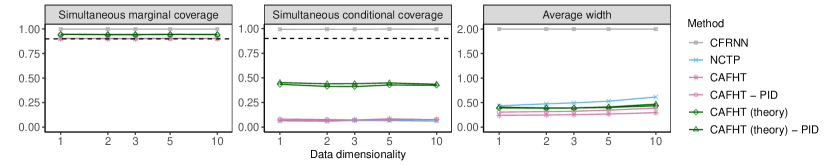
Figure 21: Performance on simulated heterogeneous trajectories of prediction bands constructed by different methods, as a function of the data dimensionality. See Table 18 for detailed results and standard errors.

Table 18: Performance on simulated heterogeneous trajectories of prediction bands constructed by different methods, as a function of the data dimensionality. The red numbers indicate smaller prediction bands or higher conditional coverage. See the corresponding plot in Figure 21.

			Simultaneous coverage
Data dimensionality	Method	Average width	Conditional-hard	Conditional-easy	Marginal
1
1	CFRNN	2.000 (0.000)	0.993 (0.001)	1.000 (0.000)	0.999 (0.000)
1	NCTP	0.435 (0.024)	0.063 (0.008)	0.996 (0.001)	0.904 (0.002)
1	CAFHT	0.241 (0.008)	0.069 (0.010)	0.993 (0.001)	0.901 (0.002)
1	CAFHT - PID	0.306 (0.019)	0.081 (0.012)	0.994 (0.001)	0.904 (0.002)
1	CAFHT (theory)	0.393 (0.004)	0.434 (0.011)	1.000 (0.000)	0.944 (0.001)
1	CAFHT (theory) - PID	0.407 (0.004)	0.452 (0.011)	1.000 (0.000)	0.946 (0.001)
2
2	CFRNN	2.000 (0.000)	0.994 (0.001)	1.000 (0.000)	0.999 (0.000)
2	NCTP	0.475 (0.027)	0.059 (0.007)	0.996 (0.001)	0.903 (0.002)
2	CAFHT	0.247 (0.008)	0.067 (0.009)	0.993 (0.001)	0.902 (0.002)
2	CAFHT - PID	0.317 (0.020)	0.077 (0.011)	0.993 (0.001)	0.902 (0.002)
2	CAFHT (theory)	0.386 (0.003)	0.413 (0.011)	1.000 (0.000)	0.942 (0.001)
2	CAFHT (theory) - PID	0.392 (0.003)	0.440 (0.010)	1.000 (0.000)	0.945 (0.001)
3
3	CFRNN	2.000 (0.000)	0.993 (0.001)	1.000 (0.000)	0.999 (0.000)
3	NCTP	0.495 (0.028)	0.068 (0.009)	0.996 (0.001)	0.904 (0.002)
3	CAFHT	0.254 (0.008)	0.073 (0.010)	0.992 (0.001)	0.901 (0.002)
3	CAFHT - PID	0.323 (0.021)	0.073 (0.010)	0.993 (0.001)	0.902 (0.002)
3	CAFHT (theory)	0.390 (0.004)	0.412 (0.013)	1.000 (0.000)	0.942 (0.002)
3	CAFHT (theory) - PID	0.392 (0.004)	0.441 (0.012)	1.000 (0.000)	0.944 (0.002)
5
5	CFRNN	2.000 (0.000)	0.995 (0.001)	1.000 (0.000)	1.000 (0.000)
5	NCTP	0.529 (0.032)	0.066 (0.009)	0.997 (0.001)	0.906 (0.002)
5	CAFHT	0.267 (0.009)	0.084 (0.012)	0.993 (0.001)	0.904 (0.002)
5	CAFHT - PID	0.346 (0.024)	0.072 (0.010)	0.993 (0.001)	0.903 (0.002)
5	CAFHT (theory)	0.401 (0.004)	0.428 (0.012)	1.000 (0.000)	0.944 (0.001)
5	CAFHT (theory) - PID	0.411 (0.004)	0.449 (0.012)	1.000 (0.000)	0.946 (0.002)
10
10	CFRNN	2.000 (0.000)	0.994 (0.001)	1.000 (0.000)	0.999 (0.000)
10	NCTP	0.615 (0.038)	0.061 (0.008)	0.997 (0.001)	0.904 (0.002)
10	CAFHT	0.295 (0.009)	0.076 (0.011)	0.993 (0.001)	0.902 (0.002)
10	CAFHT - PID	0.389 (0.027)	0.078 (0.011)	0.994 (0.001)	0.903 (0.002)
10	CAFHT (theory)	0.435 (0.004)	0.425 (0.011)	1.000 (0.000)	0.943 (0.001)
10	CAFHT (theory) - PID	0.469 (0.004)	0.435 (0.011)	1.000 (0.000)	0.944 (0.001)

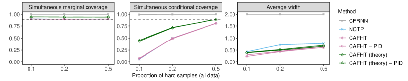
Figure 22: Performance on simulated heterogeneous trajectories of prediction bands constructed by different methods, as a function of the proportion of hard-to-predict trajectories. See Table 19 for detailed results and standard errors.

Table 19: Performance on simulated heterogeneous trajectories of prediction bands constructed by different methods, as a function of the proportion of hard-to-predict trajectories. The red numbers indicate smaller prediction bands or higher conditional coverage. See the corresponding plot in Figure 22.

			Simultaneous coverage
Proportion of hard samples (all data)	Method	Average width	Conditional-hard	Conditional-easy	Marginal
0.1
0.1	CFRNN	2.000 (0.000)	0.993 (0.001)	1.000 (0.000)	0.999 (0.000)
0.1	NCTP	0.435 (0.024)	0.063 (0.008)	0.996 (0.001)	0.904 (0.002)
0.1	CAFHT	0.241 (0.008)	0.069 (0.010)	0.993 (0.001)	0.901 (0.002)
0.1	CAFHT - PID	0.306 (0.019)	0.081 (0.012)	0.994 (0.001)	0.904 (0.002)
0.1	CAFHT (theory)	0.393 (0.004)	0.434 (0.011)	1.000 (0.000)	0.944 (0.001)
0.1	CAFHT (theory) - PID	0.407 (0.004)	0.452 (0.011)	1.000 (0.000)	0.946 (0.001)
0.2
0.2	CFRNN	2.000 (0.000)	0.996 (0.001)	1.000 (0.000)	0.999 (0.000)
0.2	NCTP	0.720 (0.006)	0.496 (0.008)	1.000 (0.000)	0.898 (0.002)
0.2	CAFHT	0.435 (0.004)	0.496 (0.010)	1.000 (0.000)	0.899 (0.002)
0.2	CAFHT - PID	0.453 (0.004)	0.488 (0.010)	1.000 (0.000)	0.897 (0.002)
0.2	CAFHT (theory)	0.497 (0.004)	0.712 (0.007)	1.000 (0.000)	0.942 (0.001)
0.2	CAFHT (theory) - PID	0.522 (0.004)	0.718 (0.006)	1.000 (0.000)	0.943 (0.001)
0.5
0.5	CFRNN	2.000 (0.000)	0.999 (0.000)	1.000 (0.000)	0.999 (0.000)
0.5	NCTP	0.776 (0.005)	0.803 (0.003)	1.000 (0.000)	0.901 (0.002)
0.5	CAFHT	0.614 (0.004)	0.805 (0.005)	1.000 (0.000)	0.902 (0.002)
0.5	CAFHT - PID	0.657 (0.005)	0.803 (0.004)	1.000 (0.000)	0.901 (0.002)
0.5	CAFHT (theory)	0.659 (0.005)	0.888 (0.003)	1.000 (0.000)	0.944 (0.002)
0.5	CAFHT (theory) - PID	0.701 (0.005)	0.883 (0.003)	1.000 (0.000)	0.941 (0.002)

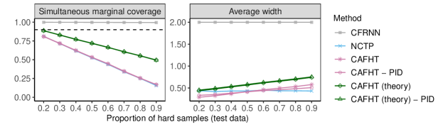
Figure 23: Performance on simulated heterogeneous trajectories of prediction bands constructed by different methods under distributional shift. The results are shown as a function of the proportion of hard-to-predict trajectories in the test data. See Table 20 for detailed results and standard errors.

Table 20: Performance on simulated heterogeneous trajectories of prediction bands constructed by different methods under distributional shift. The results are shown as a function of the proportion of hard-to-predict trajectories in the test data. The red numbers indicate higher marginal coverage. See the corresponding plot in Figure 23.

Proportion of hard samples (test data)	Method	Length	Marginal coverage
0.2
0.2	CFRNN	2.000 (0.000)	0.999 (0.000)
0.2	NCTP	0.437 (0.028)	0.811 (0.003)
0.2	CAFHT	0.289 (0.010)	0.809 (0.003)
0.2	CAFHT - PID	0.333 (0.021)	0.810 (0.004)
0.2	CAFHT (theory)	0.438 (0.005)	0.886 (0.002)
0.2	CAFHT (theory) - PID	0.453 (0.005)	0.887 (0.003)
0.3
0.3	CFRNN	2.000 (0.000)	0.998 (0.000)
0.3	NCTP	0.419 (0.027)	0.715 (0.004)
0.3	CAFHT	0.324 (0.010)	0.717 (0.004)
0.3	CAFHT - PID	0.352 (0.020)	0.717 (0.005)
0.3	CAFHT (theory)	0.478 (0.005)	0.829 (0.003)
0.3	CAFHT (theory) - PID	0.492 (0.005)	0.829 (0.004)
0.4
0.4	CFRNN	2.000 (0.000)	0.998 (0.000)
0.4	NCTP	0.432 (0.026)	0.619 (0.004)
0.4	CAFHT	0.369 (0.010)	0.624 (0.005)
0.4	CAFHT - PID	0.382 (0.019)	0.622 (0.005)
0.4	CAFHT (theory)	0.524 (0.005)	0.773 (0.004)
0.4	CAFHT (theory) - PID	0.537 (0.005)	0.770 (0.004)
0.5
0.5	CFRNN	2.000 (0.000)	0.997 (0.000)
0.5	NCTP	0.431 (0.027)	0.526 (0.005)
0.5	CAFHT	0.417 (0.011)	0.532 (0.006)
0.5	CAFHT - PID	0.414 (0.018)	0.531 (0.006)
0.5	CAFHT (theory)	0.568 (0.005)	0.719 (0.005)
0.5	CAFHT (theory) - PID	0.581 (0.006)	0.718 (0.005)
0.6
0.6	CFRNN	2.000 (0.000)	0.996 (0.001)
0.6	NCTP	0.451 (0.028)	0.438 (0.006)
0.6	CAFHT	0.460 (0.012)	0.446 (0.008)
0.6	CAFHT - PID	0.441 (0.020)	0.444 (0.008)
0.6	CAFHT (theory)	0.616 (0.006)	0.665 (0.006)
0.6	CAFHT (theory) - PID	0.627 (0.006)	0.663 (0.007)
0.7
0.7	CFRNN	2.000 (0.000)	0.996 (0.001)
0.7	NCTP	0.436 (0.027)	0.340 (0.006)
0.7	CAFHT	0.497 (0.012)	0.347 (0.008)
0.7	CAFHT - PID	0.459 (0.020)	0.343 (0.008)
0.7	CAFHT (theory)	0.655 (0.007)	0.605 (0.007)
0.7	CAFHT (theory) - PID	0.667 (0.007)	0.607 (0.007)
0.8
0.8	CFRNN	2.000 (0.000)	0.996 (0.001)
0.8	NCTP	0.437 (0.027)	0.252 (0.007)
0.8	CAFHT	0.533 (0.012)	0.255 (0.009)
0.8	CAFHT - PID	0.484 (0.020)	0.253 (0.009)
0.8	CAFHT (theory)	0.697 (0.007)	0.553 (0.008)
0.8	CAFHT (theory) - PID	0.709 (0.007)	0.553 (0.009)
0.9
0.9	CFRNN	2.000 (0.000)	0.995 (0.001)
0.9	NCTP	0.432 (0.027)	0.157 (0.007)
0.9	CAFHT	0.578 (0.013)	0.168 (0.010)
0.9	CAFHT - PID	0.508 (0.022)	0.168 (0.011)
0.9	CAFHT (theory)	0.742 (0.007)	0.496 (0.009)
0.9	CAFHT (theory) - PID	0.754 (0.007)	0.493 (0.010)

E.2 Real Data

In this subsection, we present the experimental results of the pedestrian data described in 4. Recall that we preprocess the dataset by adding heteroskedasticity such that $10\%$ of the data are designed to be hard-to-predict by adding a random noise follows $N(0,\sigma_{t}^{2})$, where $\sigma_{t}^{2}\propto t\cdot\text{noise level}$. The easy-to-predict data are added a random noise with $\sigma_{t}^{2}\propto t$. By default, noise level = 10.

Similar to the previous section, we first demonstrate the main result by using the CAFHT method with ACI and multiplicative scores as the main method to be compared with the benchmark methods CFRNN and NCTP. The results after adding the dynamic noise profile to the data are presented here for demonstrative purposes.

E.2.1 Main Results — Comparing CFRNN, NCTP, and the Main Implementation of CAFHT

Figure 5 and Table 21 show the average performance on pedestrian heterogeneous trajectories of prediction bands constructed by different methods, as a function of the total number of training and calibration trajectories. The number of trajectories is varied between 200 and 10,00. All methods achieve 90% simultaneous marginal coverage. Our method (CAFHT) leads to more informative bands with lower average width and higher conditional coverage.

The results of another experiment in which the noise level is varied from 5 to 50 are presented in Figure 24 and Table 22. Again, we observe that, even though as noise level increases and the conditional coverage for CAFHT decreases, the CAFHT consistently produces the smallest prediction bands.

Table 21: Performance on heterogeneous pedestrian trajectories of conformal prediction bands constructed by different methods, as a function of the total number of training and calibration trajectories. The red numbers indicate smaller prediction bands or higher conditional coverage. See the corresponding plot in Figure 5.

			Coverage
Sample size	Method	Length	Marginal	Conditional-easy	Conditional-hard
200
200	CFRNN	2.000 (0.000)	1.000 (0.000)	1.000 (0.000)	1.000 (0.000)
200	NCTP	0.829 (0.033)	0.916 (0.004)	0.990 (0.003)	0.274 (0.025)
200	CAFHT	0.344 (0.006)	0.914 (0.006)	0.968 (0.004)	0.445 (0.027)
500
500	CFRNN	2.000 (0.000)	1.000 (0.000)	1.000 (0.000)	1.000 (0.000)
500	NCTP	0.695 (0.024)	0.912 (0.003)	0.996 (0.001)	0.185 (0.018)
500	CAFHT	0.305 (0.004)	0.901 (0.004)	0.973 (0.002)	0.276 (0.018)
1000
1000	CFRNN	2.000 (0.000)	1.000 (0.000)	1.000 (0.000)	1.000 (0.000)
1000	NCTP	0.524 (0.023)	0.900 (0.002)	0.993 (0.001)	0.094 (0.012)
1000	CAFHT	0.299 (0.003)	0.903 (0.003)	0.978 (0.002)	0.242 (0.013)

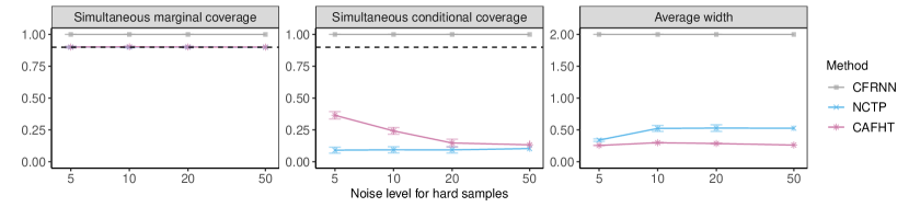
Figure 24: Performance on heterogeneous pedestrian trajectories of conformal prediction bands constructed by different methods, as a function of the noise level.

Table 22: Performance on heterogeneous pedestrian trajectories of conformal prediction bands constructed by different methods, as a function of the noise level. The red numbers indicate smaller prediction bands or higher conditional coverage. See the corresponding plot in Figure 24.

			Coverage
Noise level for hard samples	Method	Length	Marginal	Conditional-easy	Conditional-hard
5
5	CFRNN	2.000 (0.000)	1.000 (0.000)	1.000 (0.000)	1.000 (0.000)
5	NCTP	0.340 (0.010)	0.900 (0.003)	0.993 (0.001)	0.091 (0.012)
5	CAFHT	0.257 (0.002)	0.901 (0.003)	0.963 (0.002)	0.365 (0.014)
10
10	CFRNN	2.000 (0.000)	1.000 (0.000)	1.000 (0.000)	1.000 (0.000)
10	NCTP	0.524 (0.023)	0.900 (0.002)	0.993 (0.001)	0.094 (0.012)
10	CAFHT	0.299 (0.003)	0.903 (0.003)	0.978 (0.002)	0.242 (0.013)
20
20	CFRNN	2.000 (0.000)	1.000 (0.000)	1.000 (0.000)	1.000 (0.000)
20	NCTP	0.529 (0.026)	0.901 (0.003)	0.993 (0.001)	0.093 (0.012)
20	CAFHT	0.286 (0.004)	0.901 (0.003)	0.988 (0.001)	0.147 (0.015)
50
50	CFRNN	2.000 (0.000)	1.000 (0.000)	1.000 (0.000)	1.000 (0.000)
50	NCTP	0.526 (0.021)	0.900 (0.003)	0.991 (0.001)	0.103 (0.012)
50	CAFHT	0.262 (0.006)	0.900 (0.003)	0.989 (0.002)	0.133 (0.017)

E.2.2 Supplementary Results — Comparing Different CAFHT Implementations

CAFHT - multiplicative scores

The results of CAFHT methods with multiplicative conformity scores (6) are first presented in Figures 25–26 and Tables 23–24.

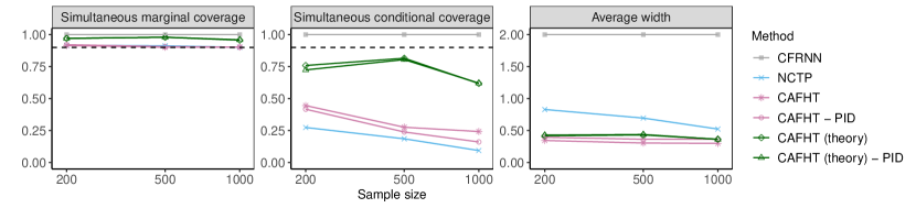
Figure 25: Performance on heterogeneous pedestrian trajectories of conformal prediction bands constructed by different methods, as a function of the total number of training and calibration trajectories.

Table 23: Performance on heterogeneous pedestrian trajectories of conformal prediction bands constructed by different methods, as a function of the total number of training and calibration trajectories. The red numbers indicate smaller prediction bands or higher conditional coverage. See the corresponding plot in Figure 25.

			Coverage
Sample size	Method	Length	Marginal	Conditional-easy	Conditional-hard
200
200	CFRNN	2.000 (0.000)	1.000 (0.000)	1.000 (0.000)	1.000 (0.000)
200	NCTP	0.829 (0.033)	0.916 (0.004)	0.990 (0.003)	0.274 (0.025)
200	CAFHT	0.344 (0.006)	0.914 (0.006)	0.968 (0.004)	0.445 (0.027)
200	CAFHT - PID	0.395 (0.021)	0.921 (0.006)	0.979 (0.004)	0.417 (0.030)
200	CAFHT (theory)	0.418 (0.006)	0.971 (0.002)	0.995 (0.001)	0.759 (0.017)
200	CAFHT (theory) - PID	0.429 (0.007)	0.970 (0.002)	0.998 (0.000)	0.724 (0.019)
500
500	CFRNN	2.000 (0.000)	1.000 (0.000)	1.000 (0.000)	1.000 (0.000)
500	NCTP	0.695 (0.024)	0.912 (0.003)	0.996 (0.001)	0.185 (0.018)
500	CAFHT	0.305 (0.004)	0.901 (0.004)	0.973 (0.002)	0.276 (0.018)
500	CAFHT - PID	0.364 (0.018)	0.905 (0.004)	0.981 (0.003)	0.239 (0.021)
500	CAFHT (theory)	0.431 (0.005)	0.979 (0.001)	0.998 (0.000)	0.815 (0.012)
500	CAFHT (theory) - PID	0.438 (0.006)	0.979 (0.001)	1.000 (0.000)	0.804 (0.013)
1000
1000	CFRNN	2.000 (0.000)	1.000 (0.000)	1.000 (0.000)	1.000 (0.000)
1000	NCTP	0.524 (0.023)	0.900 (0.002)	0.993 (0.001)	0.094 (0.012)
1000	CAFHT	0.299 (0.003)	0.903 (0.003)	0.978 (0.002)	0.242 (0.013)
1000	CAFHT - PID	0.366 (0.019)	0.902 (0.003)	0.987 (0.001)	0.161 (0.015)
1000	CAFHT (theory)	0.364 (0.003)	0.957 (0.002)	0.996 (0.001)	0.618 (0.014)
1000	CAFHT (theory) - PID	0.362 (0.003)	0.959 (0.002)	0.998 (0.000)	0.620 (0.013)

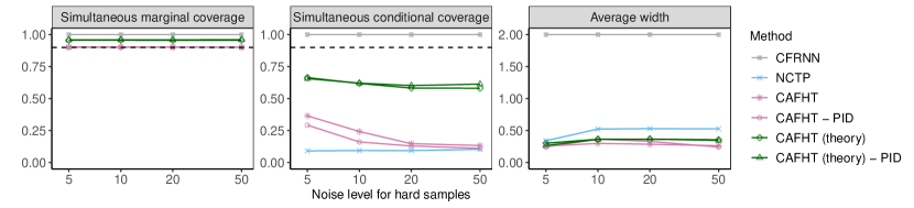
Figure 26: Performance on heterogeneous pedestrian trajectories of conformal prediction bands constructed by different methods, as a function of the noise level.

Table 24: Performance on heterogeneous pedestrian trajectories of conformal prediction bands constructed by different methods, as a function of the noise level. The red numbers indicate smaller prediction bands or higher conditional coverage. See the corresponding plot in Figure 26.

			Coverage
Noise level for hard samples	Method	Length	Marginal	Conditional-easy	Conditional-hard
5
5	CFRNN	2.000 (0.000)	1.000 (0.000)	1.000 (0.000)	1.000 (0.000)
5	NCTP	0.340 (0.010)	0.900 (0.003)	0.993 (0.001)	0.091 (0.012)
5	CAFHT	0.257 (0.002)	0.901 (0.003)	0.963 (0.002)	0.365 (0.014)
5	CAFHT - PID	0.244 (0.007)	0.904 (0.003)	0.974 (0.002)	0.292 (0.017)
5	CAFHT (theory)	0.303 (0.002)	0.957 (0.002)	0.990 (0.001)	0.664 (0.012)
5	CAFHT (theory) - PID	0.266 (0.002)	0.958 (0.002)	0.993 (0.001)	0.656 (0.013)
10
10	CFRNN	2.000 (0.000)	1.000 (0.000)	1.000 (0.000)	1.000 (0.000)
10	NCTP	0.524 (0.023)	0.900 (0.002)	0.993 (0.001)	0.094 (0.012)
10	CAFHT	0.299 (0.003)	0.903 (0.003)	0.978 (0.002)	0.242 (0.013)
10	CAFHT - PID	0.366 (0.019)	0.902 (0.003)	0.987 (0.001)	0.161 (0.015)
10	CAFHT (theory)	0.364 (0.003)	0.957 (0.002)	0.996 (0.001)	0.618 (0.014)
10	CAFHT (theory) - PID	0.362 (0.003)	0.959 (0.002)	0.998 (0.000)	0.620 (0.013)
20
20	CFRNN	2.000 (0.000)	1.000 (0.000)	1.000 (0.000)	1.000 (0.000)
20	NCTP	0.529 (0.026)	0.901 (0.003)	0.993 (0.001)	0.093 (0.012)
20	CAFHT	0.286 (0.004)	0.901 (0.003)	0.988 (0.001)	0.147 (0.015)
20	CAFHT - PID	0.331 (0.018)	0.903 (0.003)	0.992 (0.001)	0.129 (0.016)
20	CAFHT (theory)	0.366 (0.003)	0.955 (0.002)	0.999 (0.000)	0.582 (0.015)
20	CAFHT (theory) - PID	0.365 (0.004)	0.959 (0.002)	1.000 (0.000)	0.602 (0.015)
50
50	CFRNN	2.000 (0.000)	1.000 (0.000)	1.000 (0.000)	1.000 (0.000)
50	NCTP	0.526 (0.021)	0.900 (0.003)	0.991 (0.001)	0.103 (0.012)
50	CAFHT	0.262 (0.006)	0.900 (0.003)	0.989 (0.002)	0.133 (0.017)
50	CAFHT - PID	0.242 (0.011)	0.901 (0.003)	0.993 (0.001)	0.111 (0.015)
50	CAFHT (theory)	0.356 (0.003)	0.956 (0.002)	0.999 (0.000)	0.581 (0.014)
50	CAFHT (theory) - PID	0.346 (0.004)	0.960 (0.002)	1.000 (0.000)	0.613 (0.015)

CAFHT — Additive Scores

The results of CAFHT methods with additive conformity scores (3) are presented in Figures 27–28 and Tables 25–26.

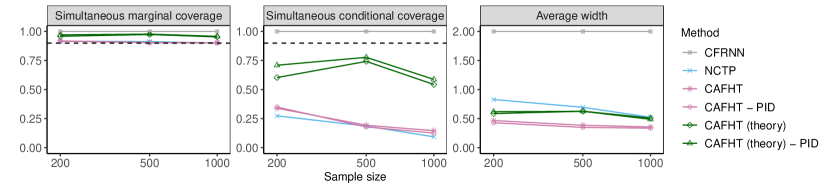
Figure 27: Performance on heterogeneous pedestrian trajectories of conformal prediction bands constructed by different methods, as a function of the total number of training and calibration trajectories.

Table 25: Performance on heterogeneous pedestrian trajectories of conformal prediction bands constructed by different methods, as a function of the total number of training and calibration trajectories. The red numbers indicate smaller prediction bands or higher conditional coverage. See the corresponding plot in Figure 27.

			Coverage
Sample size	Method	Length	Marginal	Conditional-easy	Conditional-hard
200
200	CFRNN	2.000 (0.000)	1.000 (0.000)	1.000 (0.000)	1.000 (0.000)
200	NCTP	0.829 (0.033)	0.916 (0.004)	0.990 (0.003)	0.274 (0.025)
200	CAFHT	0.467 (0.016)	0.919 (0.006)	0.984 (0.003)	0.339 (0.030)
200	CAFHT - PID	0.429 (0.021)	0.916 (0.006)	0.980 (0.004)	0.350 (0.034)
200	CAFHT (theory)	0.587 (0.013)	0.958 (0.003)	0.999 (0.001)	0.603 (0.023)
200	CAFHT (theory) - PID	0.618 (0.018)	0.970 (0.002)	1.000 (0.000)	0.709 (0.023)
500
500	CFRNN	2.000 (0.000)	1.000 (0.000)	1.000 (0.000)	1.000 (0.000)
500	NCTP	0.695 (0.024)	0.912 (0.003)	0.996 (0.001)	0.185 (0.018)
500	CAFHT	0.386 (0.012)	0.904 (0.004)	0.985 (0.003)	0.193 (0.021)
500	CAFHT - PID	0.349 (0.014)	0.903 (0.004)	0.986 (0.003)	0.179 (0.021)
500	CAFHT (theory)	0.627 (0.009)	0.974 (0.001)	1.000 (0.000)	0.742 (0.014)
500	CAFHT (theory) - PID	0.626 (0.013)	0.977 (0.001)	1.000 (0.000)	0.777 (0.014)
1000
1000	CFRNN	2.000 (0.000)	1.000 (0.000)	1.000 (0.000)	1.000 (0.000)
1000	NCTP	0.524 (0.023)	0.900 (0.002)	0.993 (0.001)	0.094 (0.012)
1000	CAFHT	0.357 (0.009)	0.904 (0.003)	0.992 (0.001)	0.146 (0.015)
1000	CAFHT - PID	0.336 (0.014)	0.901 (0.003)	0.991 (0.002)	0.126 (0.015)
1000	CAFHT (theory)	0.511 (0.006)	0.953 (0.002)	1.000 (0.000)	0.544 (0.014)
1000	CAFHT (theory) - PID	0.488 (0.006)	0.958 (0.001)	1.000 (0.000)	0.588 (0.013)

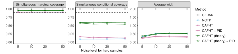
Figure 28: Performance on heterogeneous pedestrian trajectories of conformal prediction bands constructed by different methods, as a function of the noise level.

Table 26: Performance on heterogeneous pedestrian trajectories of conformal prediction bands constructed by different methods, as a function of the noise level. The red numbers indicate smaller prediction bands or higher conditional coverage. See the corresponding plot in Figure 28.

			Coverage
Noise level for hard samples	Method	Length	Marginal	Conditional-easy	Conditional-hard
5
5	CFRNN	2.000 (0.000)	1.000 (0.000)	1.000 (0.000)	1.000 (0.000)
5	NCTP	0.340 (0.010)	0.900 (0.003)	0.993 (0.001)	0.091 (0.012)
5	CAFHT	0.269 (0.004)	0.904 (0.003)	0.989 (0.002)	0.167 (0.017)
5	CAFHT - PID	0.224 (0.004)	0.899 (0.003)	0.983 (0.002)	0.168 (0.016)
5	CAFHT (theory)	0.373 (0.003)	0.957 (0.002)	1.000 (0.000)	0.578 (0.014)
5	CAFHT (theory) - PID	0.304 (0.003)	0.958 (0.002)	0.999 (0.000)	0.596 (0.015)
10
10	CFRNN	2.000 (0.000)	1.000 (0.000)	1.000 (0.000)	1.000 (0.000)
10	NCTP	0.524 (0.023)	0.900 (0.002)	0.993 (0.001)	0.094 (0.012)
10	CAFHT	0.357 (0.009)	0.904 (0.003)	0.992 (0.001)	0.146 (0.015)
10	CAFHT - PID	0.336 (0.014)	0.901 (0.003)	0.991 (0.002)	0.126 (0.015)
10	CAFHT (theory)	0.511 (0.006)	0.953 (0.002)	1.000 (0.000)	0.544 (0.014)
10	CAFHT (theory) - PID	0.488 (0.006)	0.958 (0.001)	1.000 (0.000)	0.588 (0.013)
20
20	CFRNN	2.000 (0.000)	1.000 (0.000)	1.000 (0.000)	1.000 (0.000)
20	NCTP	0.529 (0.026)	0.901 (0.003)	0.993 (0.001)	0.093 (0.012)
20	CAFHT	0.363 (0.011)	0.902 (0.003)	0.991 (0.002)	0.133 (0.016)
20	CAFHT - PID	0.327 (0.015)	0.904 (0.003)	0.992 (0.002)	0.140 (0.017)
20	CAFHT (theory)	0.531 (0.006)	0.954 (0.002)	1.000 (0.000)	0.551 (0.013)
20	CAFHT (theory) - PID	0.530 (0.007)	0.958 (0.001)	1.000 (0.000)	0.591 (0.013)
50
50	CFRNN	2.000 (0.000)	1.000 (0.000)	1.000 (0.000)	1.000 (0.000)
50	NCTP	0.526 (0.021)	0.900 (0.003)	0.991 (0.001)	0.103 (0.012)
50	CAFHT	0.346 (0.014)	0.901 (0.003)	0.990 (0.002)	0.130 (0.017)
50	CAFHT - PID	0.293 (0.015)	0.900 (0.003)	0.991 (0.002)	0.121 (0.015)
50	CAFHT (theory)	0.515 (0.006)	0.953 (0.002)	1.000 (0.000)	0.541 (0.015)
50	CAFHT (theory) - PID	0.525 (0.008)	0.958 (0.002)	1.000 (0.000)	0.586 (0.014)

References

- [1] Lars Lindemann, Matthew Cleaveland, Gihyun Shim and George J Pappas “Safe planning in dynamic environments using conformal prediction” In IEEE Robotics and Automation Letters IEEE, 2023
- [2] Jordan Lekeufack, Anastasios A Angelopoulos, Andrea Bajcsy, Michael I Jordan and Jitendra Malik “Conformal decision theory: Safe autonomous decisions from imperfect predictions” In arXiv preprint arXiv:2310.05921, 2023
- [3] Chen Xu, Daniel A Zuniga Vazquez, Rui Yao, Feng Qiu and Yao Xie “Wildfire modeling with point process and conformal prediction” In arXiv preprint arXiv:2207.13250, 2022
- [4] Chen Xu, Yao Xie, Daniel A Zuniga Vazquez, Rui Yao and Feng Qiu “Spatio-Temporal Wildfire Prediction using Multi-Modal Data” In IEEE Journal on Selected Areas in Information Theory IEEE, 2023
- [5] Vladimir Vovk, Alex Gammerman and Glenn Shafer “Algorithmic learning in a random world” Springer, 2005
- [6] Jing Lei, Max G’Sell, Alessandro Rinaldo, Ryan J. Tibshirani and Larry Wasserman “Distribution-free predictive inference for regression” In J. Am. Stat. Assoc. 113.523 Taylor & Francis, 2018, pp. 1094–1111
- [7] Jing Lei and Larry Wasserman “Distribution-free prediction bands for non-parametric regression” In J. R. Stat. Soc. (B) 76.1 Wiley Online Library, 2014, pp. 71–96
- [8] Yaniv Romano, Evan Patterson and Emmanuel J Candès “Conformalized quantile regression” In Advances in Neural Information Processing Systems, 2019, pp. 3538–3548
- [9] Matteo Sesia and Yaniv Romano “Conformal Prediction using Conditional Histograms” In Advances in Neural Information Processing Systems 34, 2021
- [10] Jing Lei, James Robins and Larry Wasserman “Distribution-Free Prediction Sets” In J. Am. Stat. Assoc. 108.501 Taylor & Francis, 2013, pp. 278–287
- [11] Mauricio Sadinle, Jing Lei and Larry Wasserman “Least ambiguous set-valued classifiers with bounded error levels” In J. Am. Stat. Assoc. 114.525 Taylor & Francis, 2019, pp. 223–234
- [12] Aleksandr Podkopaev and Aaditya Ramdas “Distribution-free uncertainty quantification for classification under label shift” In Uncertainty in Artificial Intelligence, 2021, pp. 844–853 PMLR
- [13] Stephen Bates, Emmanuel Candès, Lihua Lei, Yaniv Romano and Matteo Sesia “Testing for outliers with conformal p-values” In Ann. Stat. 51.1 Institute of Mathematical Statistics, 2023, pp. 149–178
- [14] Ariane Marandon, Lihua Lei, David Mary and Etienne Roquain “Machine learning meets false discovery rate” In arXiv preprint arXiv:2208.06685, 2022
- [15] Ziyi Liang, Matteo Sesia and Wenguang Sun “Integrative conformal p-values for out-of-distribution testing with labelled outliers” In J. R. Stat. Soc. (B) Oxford University Press US, 2024, pp. qkad138
- [16] Chen Xu and Yao Xie “Conformal prediction interval for dynamic time-series” In International Conference on Machine Learning, 2021, pp. 11559–11569 PMLR
- [17] Kamile Stankeviciute, Ahmed M Alaa and Mihaela Schaar “Conformal time-series forecasting” In Adv. Neural Inf. Process. Syst. 34, 2021, pp. 6216–6228
- [18] Chen Xu and Yao Xie “Sequential predictive conformal inference for time series” In International Conference on Machine Learning, 2023, pp. 38707–38727 PMLR
- [19] Niccolò Ajroldi, Jacopo Diquigiovanni, Matteo Fontana and Simone Vantini “Conformal prediction bands for two-dimensional functional time series” In Computational Statistics & Data Analysis 187 Elsevier, 2023, pp. 107821
- [20] Isaac Gibbs and Emmanuel Candès “Adaptive conformal inference under distribution shift” In Adv. Neural Inf. Process. Syst. 34, 2021, pp. 1660–1672
- [21] Isaac Gibbs and Emmanuel Candès “Conformal inference for online prediction with arbitrary distribution shifts” In arXiv preprint arXiv:2208.08401, 2022
- [22] Anastasios N Angelopoulos, Emmanuel J Candès and Ryan J Tibshirani “Conformal PID control for time series prediction” In arXiv preprint arXiv:2307.16895, 2023
- [23] Yaniv Romano, Matteo Sesia and Emmanuel J. Candès “Classification with Valid and Adaptive Coverage” In Advances in Neural Information Processing Systems 33, 2020
- [24] Bat-Sheva Einbinder, Yaniv Romano, Matteo Sesia and Yanfei Zhou “Training Uncertainty-Aware Classifiers with Conformalized Deep Learning” In Adv. Neural Inf. Process. Syst. 35, 2022
- [25] Ryan J Tibshirani, Rina Foygel Barber, Emmanuel Candes and Aaditya Ramdas “Conformal prediction under covariate shift” In Advances in neural information processing systems 32, 2019
- [26] Rina Foygel Barber, Emmanuel J Candès, Aaditya Ramdas and Ryan J Tibshirani “Conformal prediction beyond exchangeability” In arXiv preprint arXiv:2202.13415, 2022
- [27] Hongxiang Qiu, Edgar Dobriban and Eric Tchetgen “Prediction sets adaptive to unknown covariate shift” In J. R. Stat. Soc. (B), 2023
- [28] Osbert Bastani, Varun Gupta, Christopher Jung, Georgy Noarov, Ramya Ramalingam and Aaron Roth “Practical Adversarial Multivalid Conformal Prediction” In Adv. Neural Inf. Process. Syst., 2022
- [29] Margaux Zaffran, Aymeric Dieuleveut, Olivier F’eron, Yannig Goude and Julie Josse “Adaptive Conformal Predictions for Time Series” In International Conference on Machine Learning, 2022
- [30] Shai Feldman, Liran Ringel, Stephen Bates and Yaniv Romano “Achieving Risk Control in Online Learning Settings” In arXiv preprint arXiv:2307.16895, 2023
- [31] Anushri Dixit, Lars Lindemann, Skylar X Wei, Matthew Cleaveland, George J Pappas and Joel W Burdick “Adaptive conformal prediction for motion planning among dynamic agents” In Learning for Dynamics and Control Conference, 2023, pp. 300–314 PMLR
- [32] Aadyot Bhatnagar, Huan Wang, Caiming Xiong and Yu Bai “Improved online conformal prediction via strongly adaptive online learning” In Proceedings of the 40th International Conference on Machine Learning, 2023
- [33] Victor Chernozhukov, Kaspar Wüthrich and Zhu Yinchu “Exact and robust conformal inference methods for predictive machine learning with dependent data” In Conference On learning theory, 2018, pp. 732–749 PMLR
- [34] Chen Xu and Yao Xie “Conformal prediction set for time-series” In arXiv preprint arXiv:2206.07851, 2022
- [35] Martim Sousa, Ana Maria Tomé and José Moreira “A general framework for multi-step ahead adaptive conformal heteroscedastic time series forecasting” In arXiv preprint arXiv:2207.14219, 2022
- [36] Andreas Auer, Martin Gauch, Daniel Klotz and Sepp Hochreiter “Conformal Prediction for Time Series with Modern Hopfield Networks” In Adv. Neural Inf. Process. Syst., 2023
- [37] Hui Xu, Song Mei, Stephen Bates, Jonathan Taylor and Robert Tibshirani “Uncertainty Intervals for Prediction Errors in Time Series Forecasting” In arXiv preprint arXiv:2309.07435, 2023
- [38] Zhen Lin, Shubhendu Trivedi and Jimeng Sun “Conformal Prediction with Temporal Quantile Adjustments” In Adv. Neural Inf. Process. Syst., 2022
- [39] Xinyi Yu, Yiqi Zhao, Xiang Yin and Lars Lindemann “Signal Temporal Logic Control Synthesis among Uncontrollable Dynamic Agents with Conformal Prediction” In arXiv preprint arXiv:2312.04242, 2023
- [40] Matthew Cleaveland, Insup Lee, George J Pappas and Lars Lindemann “Conformal Prediction Regions for Time Series using Linear Complementarity Programming” In arXiv preprint arXiv:2304.01075, 2023
- [41] Vladimir Vovk “Conditional Validity of Inductive Conformal Predictors” In Proceedings of the Asian Conference on Machine Learning 25, 2012, pp. 475–490
- [42] Rina Foygel Barber, Emmanuel J Candès, Aaditya Ramdas and Ryan J Tibshirani “The limits of distribution-free conditional predictive inference” In Information and Inference 10.2 Oxford University Press, 2021, pp. 455–482
- [43] Rafael Izbicki, Gilson Shimizu and Rafael Stern “Flexible distribution-free conditional predictive bands using density estimators” In International Conference on Artificial Intelligence and Statistics, 2020, pp. 3068–3077 PMLR
- [44] Maxime Cauchois, Suyash Gupta and John C Duchi “Knowing what you know: valid and validated confidence sets in multiclass and multilabel prediction” In J. Mach. Learn. Res., 22.1, 2021, pp. 3681–3722
- [45] Matteo Sesia, Stefano Favaro and Edgar Dobriban “Conformal Frequency Estimation with Sketched Data under Relaxed Exchangeability” In arXiv preprint arXiv:2211.04612, 2022
- [46] Yaniv Romano, Rina Foygel Barber, Chiara Sabatti and Emmanuel Candès “With Malice Toward None: Assessing Uncertainty via Equalized Coverage” In Harvard Data Science Review, 2020
- [47] Sepp Hochreiter and Jürgen Schmidhuber “Long short-term memory” In Neural computation 9.8 MIT press, 1997, pp. 1735–1780
- [48] Alexandre Alahi, Kratarth Goel, Vignesh Ramanathan, Alexandre Robicquet, Li Fei-Fei and Silvio Savarese “Social lstm: Human trajectory prediction in crowded spaces” In Proceedings of the IEEE conference on computer vision and pattern recognition, 2016, pp. 961–971
- [49] Nigamaa Nayakanti, Rami Al-Rfou, Aurick Zhou, Kratarth Goel, Khaled S Refaat and Benjamin Sapp “Wayformer: Motion forecasting via simple & efficient attention networks” In arXiv preprint arXiv:2207.05844, 2022
- [50] Zikang Zhou, Jianping Wang, Yung-Hui Li and Yu-Kai Huang “Query-Centric Trajectory Prediction” In Proceedings of the IEEE/CVF Conference on Computer Vision and Pattern Recognition, 2023, pp. 17863–17873
- [51] Skylar X. Wei, Anushri Dixit, Shashank Tomar and Joel W. Burdick “Moving Obstacle Avoidance: A Data-Driven Risk-Aware Approach” In IEEE Control Systems Letters 7, 2023, pp. 289–294
- [52] Jing Lei, Max G’Sell, Alessandro Rinaldo, Ryan J. Tibshirani and Larry Wasserman “Distribution-free predictive inference for regression” In J. Am. Stat. Assoc. 113.523 Taylor & Francis, 2018, pp. 1094–1111
- [53] Yachong Yang and Arun Kumar Kuchibhotla “Finite-sample efficient conformal prediction” In arXiv preprint arXiv:2104.13871, 2021
- [54] Ziyi Liang, Yanfei Zhou and Matteo Sesia “Conformal inference is (almost) free for neural networks trained with early stopping” In Proceedings of the 40th International Conference on Machine Learning, 2023
- [55] Jur Van den Berg, Ming Lin and Dinesh Manocha “Reciprocal velocity obstacles for real-time multi-agent navigation” In 2008 IEEE international conference on robotics and automation, 2008, pp. 1928–1935 IEEE
- [56] Matteo Sesia and Emmanuel J Candès “A comparison of some conformal quantile regression methods” In Stat 9.1 Wiley Online Library, 2020
- [57] Vladimir Vovk “Cross-conformal predictors” In Annals of Mathematics and Artificial Intelligence 74.1-2 Springer, 2015, pp. 9–28
- [58] Rina Foygel Barber, Emmanuel J Candès, Aaditya Ramdas and Ryan J Tibshirani “Predictive inference with the jackknife+” In Ann. Stat. 49.1 Institute of Mathematical Statistics, 2021, pp. 486–507
- [59] Meshi Bashari, Amir Epstein, Yaniv Romano and Matteo Sesia “Derandomized novelty detection with FDR control via conformal e-values” In arXiv preprint arXiv:2302.07294, 2023