Advanced fuel fusion, phase space engineering, and structure-preserving geometric algorithms

Abstract

Non-thermal advanced fuel fusion trades the requirement of a large amount of recirculating tritium in the system for that of large recirculating power. Phase space engineering technologies utilizing externally injected electromagnetic fields can be applied to meet the challenge of maintaining non-thermal particle distributions at a reasonable cost. The physical processes of the phase space engineering are studied from a theoretical and algorithmic perspective. It is emphasized that the operational space of phase space engineering is limited by the underpinning symplectic dynamics of charged particles. The phase space incompressibility according to the Liouville theorem is just one of many constraints, and Gromov’s non-squeezing theorem determines the minimum footprints of the charged particles on every conjugate phase space plane. In this sense and level of sophistication, the mathematical abstraction of phase space engineering is symplectic topology. To simulate the processes of phase space engineering, such as the Maxwell demon and electromagnetic energy extraction, and to accurately calculate the minimum footprints of charged particles, recently developed structure-preserving geometric algorithms can be used. The family of algorithms conserves exactly, on discretized spacetime, symplecticity and thus incompressibility, non-squeezability, and symplectic capacities. The algorithms apply to the dynamics of charged particles under the influence of external electromagnetic fields as well as the charged particle-electromagnetic field system governed by the Vlasov-Maxwell equations.

I Introduction

Among all light-ion nuclear fusion reactions that are potentially suitable for energy production, deuterium-tritium (D-T) fusion is advantageous in terms of having the largest cross-section and lowest energy for peaked cross-section. D-T fusion reactions can be sustained in a confined, thermalized plasma consisting of deuterium and tritium ions at 10KeV temperature without significant radiation loss. This is desirable since fusion cross-sections are always much smaller than those of Coulomb scatterings between charged particles, and the fusion plasma thermalizes quickly before fusion unless powerful external electromagnetic fields are applied to maintain the non-thermal particle distributions. The cross-sections for advanced fuel fusion reactions [1, 2, 3, 4], such as the deuterium-helium-3 (D-He3) fusion and proton-boron-11 (P-B11) fusion, peak at much higher energies. These fusion reactions are difficult to sustain in thermalized plasmas because of the significantly increased radiation loss of energy at higher temperatures [3, 5]. From the perspective of reducing transport due to collisions and turbulence, D-T fusion is also favorable because of the lower temperature required.

The disadvantages of D-T fusion are also prominent. First, the fusion energy is carried by 14MeV neutrons, which damage the first wall and other necessary plasma-facing hardware, such as RF antennas. Moreover, magnetic confinement devices such as tokamaks or stellarators will require massive superconducting magnets, which will need to be fully shielded from these neutrons. Much effort has been directed toward developing materials that can resist the energetic fusion neutrons. There is another difficulty. D-T fusion power plants are believed to be clean and have an unlimited supply of fuel. This is certainly true for deuterium. But for tritium, fuel self-sustainability is still an engineering challenge [6, 7]. Assuming initial tritium inventory is available through other venues, tritium breeding using fusion neutrons and lithium-6 is the currently envisioned solution for tritium self-sustainability. However, this requires a near-perfect tritium recycling and recovery rate, given the tritium burning fraction and tritium breeding ratio currently achievable. For an analogy to draw below, let $\beta$ denote the tritium burning fraction in one particle confinement time, $r$ the tritium breeding return (1+$r$ is the tritium breeding ratio), and $l$ the tritium recycling and recovery loss rate. For simplicity, we use the same loss rate for the tritium recycling from divertors/first walls and tritium recovery from the breeder blankets. Tritium self-sustainability means $\beta+(1-\beta)l<\beta(1+r)(1-l)$, which, when $\beta$ and $l$ are small, simplifies to

$$l<\beta r.$$ (1)

For the typical values of $\beta=1\%$ and $r=10\%$ [6, 7], the tritium recycling and recovery loss rate $l$ must be less than $0.1\%.$ This is a stringent requirement imposed by the large amount of recirculating tritium in the system associated with the low tritium burning ratio (see Fig. 1). Even if a near-perfect recycling and recovery rate is achievable, it translates to expansive capital and operational costs.

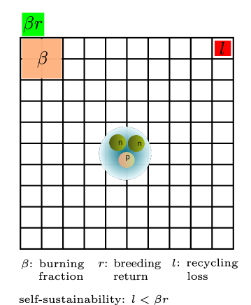
Figure 1: Tritium self-sustainability is still an engineering challenge. For the tritium burning fraction and breeding return currently achievable, there is a large amount of recirculating tritium in the system, and the required tritium recycling and recovery rate is in the range of 99.9%.

For commercial fusion energy production, advanced fuel fusion using D-He3 or P-B11 has been considered as a possible alternative with certain advantages [1, 8, 2, 3, 9, 10, 11, 12, 13]. In addition to being tritium-free, D-He3 and P-B11 reactions are also almost aneutronic, removing the need to develop neutron-resisting materials. In exchange for these two major advantages, advanced fuel fusion needs to be operated in a non-thermal setting, for the reason discussed above, and the challenge is how to maintain the non-thermal particle distributions and the associated recirculating power at an affordable cost [1, 8, 14, 2, 15]. In this sense, advanced fuel fusion trades the requirement of a large amount recirculating tritium for that of large recirculating power. It is reasonable to expect that recirculating power is easier to generate and maintain in comparison. To meet the challenge, innovative phase space engineering using electromagnetic fields can be applied [16, 17, 18, 19, 20, 21]. For charged particles in ionized plasmas, injecting high-frequency electromagnetic fields seems to be the only way to manipulate phase space distributions faster than the collisional thermalization, and such methods have been extensively investigated for achieving hot ion modes via $\alpha$-channeling in D-T fusion [22, 23, 24, 25, 26]. In the present study, we analyze the physics of phase space engineering from a theoretical and algorithmic perspective. In particular, we emphasize the phase space constraints imposed by the Hamiltonian nature of the dynamics and discuss structure-preserving geometric algorithms that are indispensable in the study and design of phase space engineering techniques. In Sec. II, we discuss the need for phase space engineering for non-thermal advanced fuel fusion. Symplectic dynamics of charged particles, the underpinning physics of phase space engineering, and the associated phase space constraints are analyzed in Sec. III. Structure-preserving geometric algorithms suitable for phase space engineering are presented in Sec. IV.

II Phase space engineering for non-thermal advanced fuel fusion

Even for the thermal D-T fusion, the fusion plasma is not fully thermalized. Phase space engineering has been utilized to heat plasmas [27, 28], suppress instabilities [29, 30, 31, 32], drive current [33], and channel the energy of $\alpha$-particles for hot ion modes [22, 23, 24, 25, 26]. In particle accelerators, phase space engineering is routinely used to control the properties of charged particle beams [34, 35, 36, 37].

For non-thermal advanced fuel fusion, large recirculating power exists in the system to maintain the non-thermal distributions of particles, which does not necessarily entail significant energy loss if enough attention is paid to preserve the power flow. An example is the energy-recovering accelerator technology [38]. If the success of D-T fusion energy is only possible with lossless tritium recirculation in the system, non-thermal advanced fuel fusion depends on phase space engineering that can sustain efficient recirculating power. Let’s demonstrate conceptually how an RF field-driven Maxwell demon [39, 40, 41, 42, 43, 22, 44, 45, 46] can be utilized to maintain the directed energy of a fusing ion beam. In the co-moving frame of the beam, a Maxwell demon is implemented as a one-way door that allows ions with forward velocity to pass through but reflects ions with backward velocity, see Fig. 2. The one-way door guarded by the demon can also be called a one-way wall. It converts the thermal energy into the directed kinetic energy of the beam. In this process, the entropy of the ion beam is decreased, which is associated with certain energy costs and increased entropy of the entire system including the external hardware generating the RF field. The technical challenge is to minimize the cost within the operational space allowed by physics.

Figure 2: A Maxwell demon guarding a one-way door. The blue balls inside (representing backward-moving particles) are bounced back at the door, and the red balls outside (representing forward-moving particles) are allowed in.

Not all phase space manipulations are possible if the Maxwell demon was driven by electromagnetic fields. For example, the phase space volume of the ions needs to be conserved according to the Liouville theorem, which is known as phase-space incompressibility (see Sec. III). When the backward-moving ions are pushed forward by the demon, they have to occupy the same volume in the left part of the phase space as shown in Fig. 3(a). If the operation is confined in the $(x,v_{x})$ plane, incompressibility rules out the possibility of forming a cold, focused, energetic beam as shown in Fig.3(b), which would be ideal for fusion reactions.

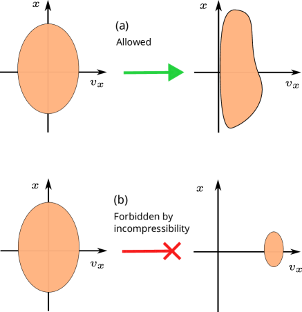
Figure 3: Not all phase space manipulations by a Maxwell demon driven by electromagnetic fields are possible. The phase space volume of the ions needs to be conserved according to the Liouville theorem. If the operation is confined in the $(x,v_{x})$ plane, incompressibility rules out the possibility of forming a cold, focused, energetic beam as shown in (b), which would be ideal for fusion reactions.

One of the advantages of aneutronic fusion is that the fusion energy is released in the form of kinetic energy carried by charged particles, and the fusion energy can be extracted directly and efficiently as electromagnetic energy. However, because the kinetic energy of the fusing ions is much smaller than the fusion energy released, the released energy is largely thermalized and occupies a certain phase space volume that needs to be conserved during the direct energy extraction via electromagnetic channels. For a given distribution of fusion products, e.g., $\alpha$-particles in the P-B11 fusion, what is the maximum fusion energy that can be extracted electromagnetically [47, 48, 49, 50]? Or equivalently, what is the ground state of the system via electromagnetic channels? Because of the phase-space incompressibility, the ground state energy is not zero.

Gardner studied the ground state of a phase space distribution accessible by all possible volume-preserving maps of phase space [51]. Let $f_{0}(\boldsymbol{x},\boldsymbol{v})$ denote the initial distribution and $\phi(\boldsymbol{x})$ an external potential. Gardner showed that the ground state accessible via volume-preserving maps is $f_{1}(\phi(\boldsymbol{x})+mv^{2}/2)$, where $f_{1}$ is a function of one scalar argument satisfying: (1) $f$ is monotonically decreasing and (2) for any $\xi>0$, the phase space volume of the region where $f_{1}(\phi(\boldsymbol{x})+mv^{2}/2)>\xi$ is equal to the phase space volume of the region where $f_{0}(\boldsymbol{x},\boldsymbol{v})>\xi$. The function $f_{1}$ is uniquely determined. Let’s call this ground state accessible via volume-preserving maps Gardner ground state. Intuitively, the Gardner ground state is reached by “doing a Lebesgue integral”, which can be explained as follows. Suppose a coin purse dropped and the coins inside scattered on the floor. There are two ways to pick up the coins and count your assets. You can pick up all the coins on the first square foot of the floor, then all the coins on the second square foot, and so on. This is the Riemann integral. Alternatively, you can pick up all the quarters first, then all the dimes, then all the nickels, and finally all the pennies. This is the Lebesgue integral, and in Gardner’s terminology, $\xi=25\cent,10\cent,5\cent,$ and $1\cent$. Gardner’s construction was later interpreted as Gardner re-stacking algorithm [52, 53]. The algorithm moves all the quarters to the center of the floor without changing the size of their footprints, then all the dimes to the region next to the quarters, and so on. See Fig. 4.

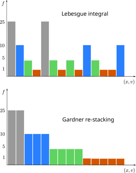
Figure 4: Gardner ground state is reached by “doing a Lebesgue integral”.

It turns out that incompressibility, or phase space volume conservation, is just one of many constraints in phase space. Another important constraint is known as non-squeezability, which is a consequence of the symplectic nature of the Hamiltonian dynamics of charged particles under the influence of electromagnetic fields. To design effective phase space engineering schemes, it is crucial to understand these dynamic constraints and adopt structure-preserving simulation algorithms that preserve these constraints. As we will see, the Gardner ground state may not be accessible by the Hamiltonian dynamics of charged particles under the influence of externally injected or self-consistently generated electromagnetic fields.

III Symplectic dynamics of charged particles — the physics of phase space engineering

In this section, we briefly describe the constraints of phase space dynamics as imposed by the law of physics and the relevance to phase space engineering. The dynamics of charged particles under the influence of an external or self-consistently generated electromagnetic field is governed by Hamilton’s equation,

$$\dot{x}^{i} =\frac{\partial H}{\partial p_{i}},\,\,\,\dot{p}_{i}=-\frac{\partial H}{\partial x^{i}},\,\,\,i=1,2,3,$$ (2)

where $H=H(x^{i},p_{i},t)$ is the Hamiltonian function. For a general electromagnetic field on spacetime specified by 4-potential $(\phi(\boldsymbol{x},t),\boldsymbol{A}(\boldsymbol{x},t)),$

$$\boldsymbol{p} =m\dot{\boldsymbol{x}}+\frac{q}{c}\boldsymbol{A}(\boldsymbol{x},t),$$ (3)

$$H =\frac{1}{2m}\left(\boldsymbol{p}-\frac{q}{c}\boldsymbol{A}(\boldsymbol{x},t)\right)^{2}+q\phi(\boldsymbol{x},t).$$ (4)

Here, we have taken the non-relativistic limit of $H$ for simplified presentation. The dynamics according to Eqs. (2)-(4) is given by a solution map

$$\varphi_{t}:\boldsymbol{z}(0)=\left(\boldsymbol{x}(0),\boldsymbol{p}(0)\right)\mapsto\boldsymbol{z}(t)=\left(\boldsymbol{x}(t),\boldsymbol{p}(t)\right).$$ (5)

It is easy to verify that the solution map $\varphi_{t}$ is symplectic, which, by definition, means that the Jacobian matrix of $\varphi_{t}$,

$$D\varphi_{t}\equiv\frac{\partial\varphi_{t}(\boldsymbol{z})}{\partial\boldsymbol{z}},$$ (6)

is symplectic.

In general, a $2n\times 2n$ matrix $S$ is called symplectic if $S^{T}JS=J,$ where

$$J=\left(\begin{array}[]{cc}0&I_{n\times n}\\ -I_{n\times n}&0\end{array}\right),$$ (7)

which defines an almost complex structure on $\mathbb{R}^{2n},$ i.e., $J:\mathbb{R}^{2n}\rightarrow\mathbb{R}^{2n}$ and $J^{2}=-1.$ More fundamentally, the symplecticity of the solution map $\varphi_{t}$ is a geometric property. The geometric form of the canonical Hamilton’s equation in $\mathbb{R}^{2n}$ is

$$i_{\left(\dot{\boldsymbol{x}},\dot{\boldsymbol{p}}\right)}\Omega=dH,$$ (8)

where

$$\Omega\equiv-d\gamma=-d\left(\sum_{i=1}^{n}p_{i}dx^{i}\right)$$ (9)

is the canonical symplectic form. In Eq. (8), “$i$” denotes inner product between the 2-form $\Omega$ and the vector field $\left(\dot{\boldsymbol{x}},\dot{\boldsymbol{p}}\right)$, and in Eq. (9) “$d$” denotes exterior derivative.

The solution map $\varphi_{t}$ being symplectic means geometrically that $\Omega$ is an invariant of the dynamics, i.e.,

$$\varphi_{t}^{*}\Omega=\Omega,$$ (10)

where $\varphi_{t}^{*}$ denotes the pullback by $\varphi_{t}$. An immediate consequence of Eq. (10) is the volume-form conservation [54],

$$\varphi_{t}^{*} \Lambda^{2n}=\Lambda^{2n},$$ (11)

where

$$\Lambda^{2n}\equiv-\frac{(-1)^{n(n-1)/2}\Omega\wedge\cdots\wedge\Omega}{n!}\text{\,\, ({\hbox{n}} {\hbox{\text{times)},}}}$$ (12)

is the volume-form defined by the symplectic 2-form $\Omega$ in the $2n$ dimensional phase space. Equation (11) is the well-known Liouville theorem in the geometric form. Note that the dimension of $\Omega$, as a 2-form on $\mathbb{R}^{2n},$ is $n(2n-1),$ and the dimension of $\Lambda^{2n}$ is 1. Volume conservation (11), or incompressibility is necessary but not sufficient for symplecticity (10).

One may be content with the volume conservation as stated in the classical Liouville theorem and question the importance of symplecticity. The fact is that from the viewpoint of physics, phase space volume can only be meaningfully defined through the symplectic 2-form $\Omega$. Recall that length, area, and volume in spacetime can only be defined by the metric tensor that is determined by Einstein’s equation. However, the spacetime metric tensor does not define a volume-form in phase space, the symplectic 2-form $\Omega$ does [55, 56]. At the fundamental level, phase space volume conservation is one of many properties of symplectic maps.

In addition to incompressibility (volume-preserving), the non-squeezability of symplectic maps proved by Gromov in 1985 is the most celebrated one [57, 58, 59, 60, 61, 62, 63, 64, 65]. Gromov’s non-squeezing theorem states: If there exists a symplectic map $\varphi$ in $\mathbb{R}^{2n}$ sending the ball $B^{2n}(r)$ into some cylinder $Z_{j}^{2n}(R),$ then $r\leq R.$ (See Fig. 5) Here,

$$B^{2n}(r) \equiv\left\{\left(x^{1},x^{2},...,x^{n},p_{1},p_{2},...,p_{n}\right)\left|\sum_{i=1}^{n}\left(p_{i}^{2}+x^{i2}\right)<r^{2}\right.\right\},$$ (13)

$$Z_{j}^{2n}(R) \equiv\left\{\left(x^{1},x^{2},...,x^{n},p_{1},p_{2},...,p_{n}\right)\left|p_{j}^{2}+x^{j2}<R^{2}\right.\right\}.$$ (14)

This is a strong constraint on symplectic maps considering the fact that $B^{2n}(r=R)\subset Z_{j}^{2n}(R).$ The ball $B^{2n}(R)$ is already in the cylinder $Z_{j}^{2n}(R)$, there is no need to squeeze it. But if we increase the size of the ball by an infinitesimal amount $\varepsilon$, then we can’t push the ball $B^{2n}(R+\varepsilon)$ into the cylinder $Z_{j}^{2n}(R)$ via any symplectic map.

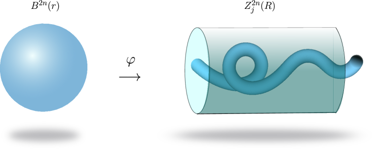
Figure 5: Gromov’s non-squeezing theorem. No symplectic map $\varphi$ can squeeze the ball $B^{2n}(r)$ into the cylinder $Z_{j}^{2n}(R)$ when $r>R.$ But for any $r\leq R,$ the ball $B^{2n}(r)$ is already inside the cylinder $Z_{j}^{2n}(R)$. The ball $B^{2n}(r)$ in phase space is “rigid”.

In $\mathbb{R}^{2n}$, the Euclidean metric $\left\langle\,,\,\right\rangle$, the canonical symplectic form $\Omega$, and the almost complex structure $J$ are compatible, i.e.,

$$\left\langle\boldsymbol{a},\boldsymbol{b}\right\rangle=\Omega(\boldsymbol{a},-J\boldsymbol{b}).$$ (15)

The distance in Eqs. (13) and (14) is measured using this metric. In addition, all maps in the present study are assumed to be diffeomorphisms (smooth) unless explicitly stated otherwise.

It is easily shown [64] that the non-squeezing theorem is equivalent to the fact that under a symplectic map $\varphi,$ the projection or footprint of $B^{2n}(r)$ on any $(x^{j},p_{j})$ plane is always larger than $\pi r^{2},$ i.e.,

$$\text{Area of }\left\{\left(x^{j},p_{j}\right)\left|\left(x^{1},x^{2},...,x^{n},p_{1},p_{2},...,p_{n}\right)\in\varphi\left(B^{2n}(r)\right)\right.\right\}\geq\pi r^{2}.$$ (16)

Non-squeezability stipulates that the phase space footprint on each $(x^{j},p_{j})$ plane $(1\leq j\leq n)$ is non-diminishing relative to an initial set that is a ball $B^{2n}(r)$ in phase space.

Non-squeezability puts strong constraints on phase space engineering. Take the example of the Maxwell demon discussed in Sec. II. Starting from a phase space ball in $\mathbb{R}^{6}$, after sending the system through a Maxwell demon in the $(x,p_{x})$ plane, we may wish to reduce the footprint of the particle system in the $(x,p_{x})$ plane to reduce the energy cost. This would be achievable by squeezing a certain amount of phase space volume across the $(y,p_{x})$ or $(z,p_{z})$ plane if phase space volume conservation were the only constraint. But, the non-squeezing theorem prohibits this type of operation. For a given initial distribution $f_{0}$, the corresponding Gardner ground state may not be accessible by symplectic maps.

If the initial set $V$ of particles in phase space is not a ball, what will be the minimum footprint in a conjugate plane $(x^{j},p_{j})$ $(1\leq j\leq n)$ under a symplectic map $\varphi$? In this case, we can search for the largest ball that can be squeezed inside $V$ by a symplectic map,

$$C_{0}(V)\equiv\sup_{\varphi\in Sym}\left\{\pi r^{2}\left|\varphi\left(B^{2n}(r)\right)\subset V\right.\right\},$$ (17)

where $Sym$ is the set of all symplectic diffeomorphisms (symplectomorphisms) in $\mathbb{R}^{2n}.$ Obviously, $C_{o}(V)$ is a symplectic invariant and can be used as a measure of the minimum footprint. Similarly, we can also search for the smallest cylinder that $V$ can be squeezed into by a symplectic map,

$$C_{1}(V)\equiv\inf_{\varphi\in Sym}\left\{\pi R^{2}\left|\varphi\left(V\right)\subset\right.Z_{j}^{2n}(R)\right\},$$ (18)

and $C_{1}(V)$ is another symplectic invariant that can be used to measure the minimum footprint. Because there exist symplectic maps to switch $(x_{j},p^{j})$ and $(x_{i},p^{i})$ for any $i$ and $j,$ the definition of $C_{1}(V)$ is independent of $j.$ According to the non-squeezing theorem,

$$C_{0}(V)<C_{1}(V).$$

Thus, for the purpose of phase space engineering, $C_{0}(V)$ and $C_{1}(V)$ can be used to obtain a good estimate of the minimum footprint on any phase space conjugate plane $(x^{j},p_{j})$. Here, $C_{0}(V)$ and $C_{1}(V)$ are examples of a family of symplectic invariants called symplectic capacities [66, 67, 59, 61, 65, 68] that characterize symplectic maps in a similar manner that phase space volume characterizes volume-preserving maps. In fact, there are infinitely many symplectic capacities. It turns out that $C_{0}(V)$ is the smallest and $C_{1}(V)$ the largest.

We now display a proof of the non-squeezing theorem for the case of linear symplectic maps to illustrate the physics related to minimum footprints and symplectic capacities. The proof is a slightly modified version of a known proof given in Refs. [65, 68]. (The proof of the general non-squeezing theorem is difficult but not inaccessible to physicists.)

Linear symplectic maps are the solutions of linear Hamiltonian systems, which are found in many branches of physics. In particular, the dynamics of high-intensity charged particle beams in accelerators, storage rings, and transport/focusing channels is governed by time-dependent linear Hamiltonian systems [37, 69, 70, 71, 72, 73, 74, 75, 76, 77]. For non-thermal fusion technologies, the dynamics of high-intensity particle beams is expected to play an important role. The solution of a linear Hamiltonian system is a linear map specified by a $2n\times 2n$ symplectic matrix $S,$

$$\varphi:\boldsymbol{z}\mapsto\bar{\boldsymbol{z}}=\varphi(\boldsymbol{z})=S\boldsymbol{z}.$$ (19)

Here, $\boldsymbol{z}=\left(x^{1},x^{2},...,x^{n},p_{1},p_{2},...,p_{n}\right).$

For linear symplectic maps, Gromov’s non-squeezing theorem reads: If there exist a symplectic matrix $S$ and an integer $j\leq n$ such that $S\left(B^{2n}(r)\right)\subset Z_{j}^{2n}(R)$, then $R\geq r.$

Without losing generality, we prove the case of $r=1$ and $j=1.$ The strategy of proof is to show that for some $\boldsymbol{z}_{0}$ on the boundary of $B^{2n}(1),$ the absolute value of the $x_{1}$ or $p^{1}$ coordinate of $S\boldsymbol{z}_{0}$ is no less than $1.$ However, by definition, $B^{2n}(1)$ is open, and we need to select a sequence of points in $B^{2n}(1)$ to approach $\boldsymbol{z}_{0}.$ Using the metric defined in Eq. (15), we select the orthonormal bases $(\boldsymbol{a},\boldsymbol{b})$ for the $(x_{1},p^{1})$ coordinates. The images of $\boldsymbol{a}$ and $\boldsymbol{b}$ under $S^{T}$ are $\bar{\boldsymbol{a}}=S^{T}\boldsymbol{a}$ and $\bar{\boldsymbol{b}}=S^{T}\boldsymbol{b}$. Consider

$$1=\Omega(\boldsymbol{a},\boldsymbol{b})=\Omega(\bar{\boldsymbol{a}},\bar{\boldsymbol{b}})=\left\langle\bar{\boldsymbol{a}},-J\bar{\boldsymbol{b}}\right\rangle\leq\left|\bar{\boldsymbol{a}}\right|\left|J\bar{\boldsymbol{b}}\right|=\left|\bar{\boldsymbol{a}}\right|\left|\bar{\boldsymbol{b}}\right|,$$ (20)

where the second equal sign is because $S^{T}$ is symplectic, and inequality is the Cauchy-Schwartz inequality. Therefore, either $\left|\bar{\boldsymbol{a}}\right|\geq 1$ or $\left|\bar{\boldsymbol{b}}\right|\geq 1$. Assume $\left|\bar{\boldsymbol{a}}\right|\geq 1$ and let

$$\boldsymbol{z}_{\varepsilon}=(1-\varepsilon)\frac{\bar{\boldsymbol{a}}}{\left|\bar{\boldsymbol{a}}\right|}\in B^{2n}(1),\quad\epsilon\in(0,1).$$ (21)

The $x^{1}$ coordinate of $S\boldsymbol{z}_{\varepsilon}$ is

$$\left\langle\boldsymbol{a},S\boldsymbol{z}_{\varepsilon}\right\rangle =\Omega(\boldsymbol{a},-JS\boldsymbol{z}_{\varepsilon})=\Omega(S^{T}\boldsymbol{a},-S^{T}JS\boldsymbol{z}_{\varepsilon})=\Omega(\bar{\boldsymbol{a}},-J\boldsymbol{z}_{\varepsilon})$$

$$=\left\langle\bar{\boldsymbol{a}},(1-\varepsilon)\frac{\bar{\boldsymbol{a}}}{\left|\bar{\boldsymbol{a}}\right|}\right\rangle=(1-\varepsilon)\left|\bar{\boldsymbol{a}}\right|\geq(1-\varepsilon).$$ (22)

If $\left|\bar{\boldsymbol{b}}\right|\geq 1$, we select $\boldsymbol{z}_{\varepsilon}=(1-\varepsilon)\bar{\boldsymbol{b}}/\left|\bar{\boldsymbol{b}}\right|\in B^{2n}(1),$ and its $p_{1}$ coordinate will be no less than $1-\varepsilon.$ Thus, the radius of $Z_{j}^{2n}(R)$ should be no less than $1-\varepsilon,$ since $S\boldsymbol{z}_{\varepsilon}\in Z_{j}^{2n}(R).$ Let $\varepsilon\rightarrow 0$ and we have $R\geq 1.$ This completes the proof.

In the proof, we find on the boundary of $B^{2n}(1)$ a point $\boldsymbol{z}_{0}$, whose footprint under any map $S$ on the $(x^{1},p_{1})$ plane sticks out the unit circle. But neither $\boldsymbol{z}_{0}$ nor $S\boldsymbol{z}_{0}$ is necessarily on the $(x^{1},p_{1})$ plane. $\boldsymbol{z}$ can be anywhere on the surface of $B^{2n}(1),$ depending on $S.$ The fact that the footprint of $S\left(B^{2n}(1)\right)$ sticks out the unit circle on the $(x^{1},p_{1})$ plane for any $S$ is attributed to the information on the entire $B^{2n}(1)$, and this situation is exactly the same for every $(x^{j},p_{j})$ plane. In terms of physics and phase space engineering, the minimum footprint of a group of particles on any $(x^{j},p_{j})$ plane is the same as measured by a symplectic capacity, which is a scalar assigned to the entire group of particles. But we have choices as to which symplectic capacity to use.

For the last topic in this section, let’s go back to the canonical Hamilton’s equation for charged particles specified by Eqs. (2)-(4). The kinetic momentum $\boldsymbol{p}$ is the sum of kinetic momentum $m\dot{\boldsymbol{x}}$ and unit-normalized vector potential $\boldsymbol{A}(\boldsymbol{x},t)$ at the particle’s location. If we choose to use $\boldsymbol{x}$ and $\boldsymbol{v}=\dot{\boldsymbol{x}}$ as the phase space coordinates, Hamilton’s equation still assumes the form of Eq. (2) except that the canonical symplectic form $\Omega$ will be replaced by a non-canonical symplectic form $\omega$, i.e.,

$$i_{\left(\dot{\boldsymbol{x}},m\dot{\boldsymbol{v}}\right)}\omega =dH,$$ (23)

$$\omega =\sum_{i=1}^{3}dx^{i}\wedge\left(mdv_{i}+\frac{q}{c}dA_{i}(\boldsymbol{x},t)\right),$$ (24)

$$H =q\phi(\boldsymbol{x},t)+\frac{1}{2}m\boldsymbol{v}^{2}.$$ (25)

It is straightforward to verify that Eqs. (23)-(25) are equivalent to the familiar equations of motion,

$$\dot{\boldsymbol{x}} =\boldsymbol{v},$$

$$\dot{\boldsymbol{v}} =\frac{q}{m}\left(\boldsymbol{E}(\boldsymbol{x},t)+\frac{1}{c}\boldsymbol{v}\times\boldsymbol{B}(\boldsymbol{x},t)\right).$$

If the phase space engineering needs to consider the electromagnetic field self-consistently generated by the fusion plasma itself, the charged particle-electromagnetic field system is an infinite dimensional non-canonical Hamiltonian system specified by the Morrison-Marsden-Weinstein (MMW) bracket [78, 79, 80, 81, 82, 83],

$$\left\{\mathcal{F},\mathcal{G}\right\} (\boldsymbol{E},\boldsymbol{B},f)=\int f\left\{\frac{\delta\mathcal{F}}{\delta f},\frac{\delta\mathcal{G}}{\delta f}\right\}_{\boldsymbol{xv}}d\boldsymbol{x}d\boldsymbol{v}$$

$$+\int\left[\frac{\delta\mathcal{F}}{\delta\boldsymbol{E}}\cdot\left(\triangledown\times\frac{\delta\mathcal{G}}{\delta\boldsymbol{B}}\right)-\frac{\delta\mathcal{G}}{\delta\boldsymbol{E}}\cdot\left(\triangledown\times\frac{\delta\mathcal{F}}{\delta\boldsymbol{B}}\right)\right]d\boldsymbol{x}$$

$$+\int\left(\frac{\delta\mathcal{F}}{\delta\boldsymbol{E}}\cdot\frac{\partial f}{\partial\boldsymbol{v}}\frac{\delta\mathcal{G}}{\delta f}-\frac{\delta\mathcal{G}}{\delta\boldsymbol{E}}\cdot\frac{\partial f}{\partial\boldsymbol{v}}\frac{\delta\mathcal{F}}{\delta f}\right)d\boldsymbol{x}d\boldsymbol{v}$$

$$+\int f\boldsymbol{B}\cdot\left(\frac{\partial}{\partial\boldsymbol{v}}\frac{\delta\mathbf{\mathrm{\mathcal{F}}}}{\delta f}\times\frac{\partial}{\partial\boldsymbol{v}}\frac{\delta\mathcal{G}}{\delta f}\right)d\boldsymbol{x}d\boldsymbol{v},$$ (26)

where $\mathcal{F}$ and $\mathcal{G}$ are functionals of the function space $\left\{(\boldsymbol{E},\boldsymbol{B},f)\left|\nabla\cdot\boldsymbol{B}=0,\nabla\cdot\boldsymbol{E}=4\pi q\int fd\boldsymbol{v}\right.\right\}$. The bracket $\{h,g\}_{\boldsymbol{xv}}$ inside the first term on the right hand side is the canonical Poisson bracket for functions $h$ and $g$ of $(\boldsymbol{x},\boldsymbol{v})$,

$$\{h,g\}_{\boldsymbol{xv}}\equiv\frac{\partial h}{\partial\boldsymbol{x}}\frac{\partial g}{\partial\boldsymbol{v}}-\frac{\partial g}{\partial\boldsymbol{x}}\frac{\partial h}{\partial\boldsymbol{v}}.$$ (27)

Hamilton’s equation for the dynamics of a functional $\mathcal{F}$ is

$$\dot{\mathcal{F}}=\left\{\mathcal{F},\mathcal{H}\right\},$$ (28)

where Hamiltonian functional is

$$\mathcal{H}(f,\boldsymbol{E},\boldsymbol{B})=\frac{m}{2}\int\boldsymbol{v}{}^{2}fd\boldsymbol{x}d\boldsymbol{v}+\frac{1}{8\pi}\int\left(\boldsymbol{E}^{2}+\boldsymbol{B}^{2}\right)d\boldsymbol{x}.$$ (29)

The equations of motion for the fields are obtained by expressing them as functionals indexed by $\boldsymbol{x}$ and $\boldsymbol{v}$,

$$f\left(\boldsymbol{x},\boldsymbol{v}\right) =\mathcal{F}\left(\boldsymbol{x},\boldsymbol{v}\right)\equiv\int f\left(\boldsymbol{x}^{\prime},\boldsymbol{v}^{\prime}\right)\delta\left(\boldsymbol{x}-\boldsymbol{x}^{\prime}\right)\delta\left(\boldsymbol{v}-\boldsymbol{v}^{\prime}\right)d\boldsymbol{x}^{\prime}d\boldsymbol{v}^{\prime},$$ (30)

$$\boldsymbol{E}\left(\boldsymbol{x}\right) =\mathcal{E}\left(\boldsymbol{x}\right)\equiv\int\boldsymbol{E}\left(\boldsymbol{x}^{\prime}\right)\delta\left(\boldsymbol{x}-\boldsymbol{x}^{\prime}\right)d\boldsymbol{x}^{\prime},$$ (31)

$$\boldsymbol{B}\left(\boldsymbol{x}\right) =\mathcal{B}\left(\boldsymbol{x}\right)\equiv\int\boldsymbol{B}\left(\boldsymbol{x}^{\prime}\right)\delta\left(\boldsymbol{x}-\boldsymbol{x}^{\prime}\right)d\boldsymbol{x}^{\prime}.$$ (32)

The Hamiton’s equation (28) for $\mathcal{F}\left(\boldsymbol{x},\boldsymbol{v}\right)$, $\mathcal{E}\left(\boldsymbol{x}\right),$ and $\mathcal{B}\left(\boldsymbol{x}\right)$ recovers the standard Vlasov-Maxwell equations,

$$\frac{\partial f}{\partial t}=-\boldsymbol{v}\cdot\frac{\partial f}{\partial\boldsymbol{x}}-\frac{q}{m}\left(\boldsymbol{E}+\frac{\boldsymbol{v}}{c}\times\boldsymbol{B}\right)\cdot\frac{\partial f}{\partial\boldsymbol{v}},$$ (33)

$$\frac{\partial\boldsymbol{E}}{\partial t}=c\nabla\times\boldsymbol{B}-4\pi\int qf\boldsymbol{v}d^{3}\boldsymbol{v}$$ (34)

$$\frac{\partial\boldsymbol{B}}{\partial t}=-c\nabla\times\boldsymbol{E}.$$ (35)

IV Structure-preserving geometric algorithms for phase space engineering

While phase space incompressibility has been well-known for centuries, phase space non-squeezability has only been established for 40 years. The associated dynamic invariants, symplectic capacities, have not been widely recognized in most physics applications. For example, Gardner’s ground state analysis for plasmas only considered the phase space incompressibility. When the non-squeezability is included in the analysis, the ground state is expected to be very different, and the ground state energy will increase. From the perspective of fusion energy production, this means less energy can be extracted via conservative electromagnetic channels. In this sense and at this level of sophistication, phase space engineering for non-thermal advanced fuel fusion is abstractly symplectic topology. Admittedly, it is difficult to directly incorporate phase space non-squeezability and other constraints of symplectic topology in analytical studies or numerical simulations of phase space engineering. For instance, the minimum footprint estimates according to Eqs. (17) and (18) are important design parameters, but it is not clear how they can be accurately calculated.

Fortunately, recent investigations in structure-preserving geometric algorithms for charged particle-electromagnetic field systems have offered a solution. The newly discovered structure-preserving geometric algorithms are able to preserve the non-canonical symplectic structures given by Eqs. (24) and (26) exactly in discretized spacetime settings. Consequently, incompressibility, non-squeezability, and symplectic capacities are preserved exactly by numerical solutions. Specifically, arbitrary high-order, explicitly solvable, non-canonical symplectic algorithms have been found for both charged particle dynamics governed by Eqs. (23)-(25) [84, 85, 86, 87, 88, 89, 90, 91] and the Vlasov-Maxwell systems governed by Eqs. (26)-(29) [92, 93, 94, 86, 95, 85, 96, 97, 98, 99, 100, 101, 102, 103, 91, 104, 105, 106, 107, 108, 109, 110]. With these structure-preserving geometric algorithms, we can numerically calculate the symplectic capacities defined in Eqs. (17) and (18) as the minimum footprints for phase space engineering designs.

In this section, we explain in detail the mechanisms by which these algorithms preserve exactly the symplecticity and thus incompressibility, non-squeezability, and symplectic capacities of the Hamiltonian systems. To be concise, we will focus only on the high-order, explicitly solvable, non-canonical symplectic algorithms for the charged particle dynamics governed by Eqs. (23)-(25).

Let $\varphi_{\Delta t}$ denote the exact solution map of Eq. (23) in a time interval $\Delta t$,

$$\varphi_{\Delta t}:\boldsymbol{z}(t)\mapsto\boldsymbol{z}(t+\Delta t)=\varphi_{\Delta t}(\boldsymbol{z}).$$ (36)

$\varphi_{\Delta t}$ is symplectic, i.e,

$$\varphi_{\Delta t}^{*}\omega=\omega.$$ (37)

Denote by $\nu_{\Delta t}$ a numerical solution map of Eq. (23) in a time interval $\Delta t$,

$$\nu_{\Delta t}:\boldsymbol{z}(t)\mapsto\widetilde{\boldsymbol{z}}(t+\Delta t)=\nu_{\Delta t}(\boldsymbol{z}).$$ (38)

$\nu_{\Delta t},$ called one-step map of the algorithm, is an approximation to $\varphi_{\Delta t}$. We would like $\nu_{\Delta t}$ to be exactly symplectic as well, i.e.,

$$\nu_{\Delta t}^{*}\omega=\omega.$$ (39)

Even though $\nu_{\Delta t}$ is not exactly the same as $\varphi_{\Delta t}$ in general, we prefer $\nu_{\Delta t}$ to come from the same family of symplectomorphisms because all important properties of Hamiltonian dynamics, such as incompressibility and non-squeezability, are associated with the symplectomorphisms as a group, instead of with a specific member of the group. An algorithm is called symplectic if its one-step map is symplectic.

For a general non-canonical symplectic system, condition (39) is difficult to satisfy unless $\nu_{\Delta t}$ is the exact solution $\varphi_{\Delta t}$. In fact, no generic symplectic algorithm exists for general non-canonical systems. But for a specific given non-canonical system, bespoke symplectic algorithms might exist. Equations (23)-(25) for charged particle dynamics are such a system. The bespoke symplectic algorithms are constructed by a Hamiltonian splitting technique.

The symplectic condition (39) is satisfied if $\nu_{\Delta t}$ is an exact solution. Of course, we can’t write down the exact solution corresponding to the $\omega$ defined by Eq. (24) and $H$ defined by Eq. (25). However, observe that for the $\omega$ defined by Eq. (24), the symplectic condition (39) is satisfied exactly by the exact solution $\varphi_{\Delta t}$ generated by any Hamiltonian function. For many simple Hamiltonian functions, the exact solution maps can be written down explicitly, and the compositions of these exact solution maps will also preserve the $\omega$ defined by Eq. (24).

If we can split the Hamiltonian $H$ defined by Eq. (25) into different parts such that the exact solution for each sub-Hamiltonian system can be written down explicitly, then these exact solutions of the sub-systems can be composed to approximate the exact solution of $H$ to arbitrary high orders, and such approximate solutions automatically satisfy the symplectic condition (39). Such a splitting was found. Specifically, we split $H$ into four sub-Hamiltonians [85, 86, 87, 90, 91] ,

$$H =H_{\phi}+H_{x}+H_{y}+H_{z},$$ (40)

$$H_{\phi} =q\phi(\boldsymbol{x},t),$$ (41)

$$H_{x} =\frac{1}{2}mv_{x}^{2},\,\,H_{y}=\frac{1}{2}mv_{y}^{2},\,\,H_{z}=\frac{1}{2}mv_{z}^{2}.$$ (42)

Here, $(x,y,z)$ are the Cartesian coordinates of the configuration space, and $(v_{x},v_{y},v_{z})$ are the corresponding velocity coordinates.

For the sub-system specified by $H_{\phi},$ Eq. (23) is

$$i_{\left(\dot{\boldsymbol{x}},m\dot{\boldsymbol{v}}\right)}\omega=q\nabla\phi(\boldsymbol{x},t),$$ (43)

which, in terms of $\dot{\boldsymbol{x}}$ and $\dot{\boldsymbol{v}}$, is

$$\dot{\boldsymbol{x}} =0,$$ (44)

$$\dot{\boldsymbol{v}} =\frac{q}{m}\boldsymbol{E}(\boldsymbol{x},t),$$ (45)

where

$$\boldsymbol{E}(\boldsymbol{x},t)=-\nabla\phi(\boldsymbol{x},t)-\frac{\partial\boldsymbol{A}(\boldsymbol{x},t)}{\partial t}.$$ (46)

Note that in Eq. (46), the time derivative of the vector potential enters through the non-canonical symplectic form $\omega$ defined in Eq. (24). The exact solution map of Eq. (43) can be explicitly written down,

$$\varphi_{\phi,\Delta t}:\begin{cases}\boldsymbol{x}(t+\Delta t)=\boldsymbol{x}(t),\\ \boldsymbol{v}(t+\Delta t)=\boldsymbol{v}(t)+\frac{q}{m}\int_{0}^{\Delta t}\boldsymbol{E}\left(\boldsymbol{x}(t),t+\tau\right)d\tau.\end{cases}$$ (47)

For the sub-system specified by $H_{x}$, Eq. (23) is

$$i_{\left(\dot{\boldsymbol{x}},m\dot{\boldsymbol{v}}\right)}\omega=mv_{x}dv_{x},$$ (48)

which is

$$\dot{x}=v_{x},\,\,\dot{y}=0,\,\,\dot{z}=0,$$ (49)

$$\dot{v_{x}}=0,\,\,\dot{v_{y}}=-\frac{q}{m}B_{z}(\boldsymbol{x},t)v_{x},\,\,\dot{v_{z}}=\frac{q}{m}B_{y}(\boldsymbol{x},t)v_{x}.$$ (50)

In Eq. (50), the magnetic field $\boldsymbol{B}(\boldsymbol{x},t)=\nabla\times\boldsymbol{A}(\boldsymbol{x},t)$ also enters through the non-canonical symplectic form $\omega$. Equations (49) and (50) are more complicated than those of $H_{\phi}.$ But the exact solution map of $H_{x}$ can also be written down explicitly [85, 86, 87, 90, 91],

$$\varphi_{x,\Delta t}:\begin{cases}x(t+\Delta t)=x(t)+v_{x}(t)\Delta t,\\ y(t+\Delta t)=y(t),\\ z(t+\Delta t)=z(t),\\ v_{x}(t+\Delta t)=v_{x}(t)\\ v_{y}(t+\Delta t)=v_{y}(t)-\frac{q}{m}\int_{0}^{\Delta t}v_{x}(t)B_{z}\left(x(t)+\tau v_{x}(t),y(t),z(t),t+\tau\right)d\tau,\\ v_{z}(t+\Delta t)=v_{z}(t)+\frac{q}{m}\int_{0}^{\Delta t}v_{x}(t)B_{y}\left(x(t)+\tau v_{x}(t),y(t),z(t),t+\tau\right)d\tau.\end{cases}$$ (51)

The exact solution maps $\varphi_{y,\Delta t}$ and $\varphi_{z,\Delta t}$ for the sub-systems $H_{y}$ and $H_{z}$ can be explicitly written down in a similar manner.

It is crucial to recognize that the exact solution maps $\varphi_{x,\Delta t}$ $\varphi_{y,\Delta t},$ and $\varphi_{z,\Delta t}$ are written down in the Cartesian coordinates. It has been shown that for an orthogonal, uniform curvilinear coordinate system $(q^{1},q^{2},q^{3})$ in $\mathbb{R}^{3}$, the exact solution for sub-system $H_{q^{i}}$ can also be written down explicitly [91]. An orthogonal coordinate system is called uniform if

$$\frac{\partial h_{i}}{\partial q^{i}}=0,\,(i=1,2,3),$$ (52)

where $h_{i}$ $(i=1,2,3)$ are the Lamé coefficients. If a curvilinear coordinate system is not orthogonal or non-uniformly orthogonal, the solution maps for the subsystem defined by $H_{q^{i}}$ can’t be written down explicitly in general [91].

Arbitrary high-order symplectic algorithms for the original Hamiltonian system (23)-(25) can be constructed from different compositions of $\varphi_{\phi,\Delta t}$, $\varphi_{x,\Delta t}$ $\varphi_{y,\Delta t},$ and $\varphi_{z,\Delta t}$. Two of the 1st-order algorithms for $H$ are

$$\nu_{\Delta t}^{(1)} =\varphi_{\phi,\Delta t}\circ\varphi_{x,\Delta t}\circ\varphi_{y,\Delta t}\circ\varphi_{z,\Delta t},$$ (53)

$$\nu_{\Delta t}^{*(1)} =\varphi_{z,\Delta t}\circ\varphi_{y,\Delta t}\circ\varphi_{x,\Delta t}\circ\varphi_{\phi,\Delta t}.$$ (54)

A 2nd-order algorithm for $H$ can be built as

$$\nu_{\Delta t}^{(2)}=\nu_{\Delta t/2}^{(1)}\circ\nu_{\Delta t/2}^{*(1)},$$ (55)

which is the familiar Strang splitting. From a given $2l$th-order algorithm $\nu_{\Delta t}^{(2l)},$ a $2(l+1)$th-order algorithm can be constructed as follows,

$$\nu_{\Delta t}^{(2l+2)} =\nu_{\alpha_{l}\Delta t}^{(2l)}\circ\nu_{\beta_{l}\Delta t}^{(2l)}\circ\nu_{\alpha_{l}\Delta t}^{(2l)},$$ (56)

$$\alpha_{l} \equiv\left(2-\frac{1}{2l+1}\right)^{-1},\thinspace\thinspace\beta_{l}\equiv 1-2\alpha_{l}.$$ (57)

As emphasized above, all these algorithms preserve exactly the symplectic structure $\omega$ defined in Eq. (24) as the exact solutions do.

In the stability analysis of algorithms when applied to linear differential ODEs with constant coefficients, algorithms are often called implicit if the derivative evaluation depends on the values of dependent variables at future time-steps. If this definition is strictly followed, the symplectic algorithms described above are implicit. However, there is no need for numerical root-finding as in standard implicit algorithms. To be precise, the algorithms developed here for charged particle dynamics are explicitly solvable, implicit, and symplectic.

These non-canonical symplectic algorithms can be used as upgrades of volume-preserving but non-symplectic algorithms [111, 112, 113, 114, 115, 116, 117, 118] for charged particle dynamics, including the widely adopted Boris algorithm [119, 120, 121, 122, 123, 124, 125, 126, 127, 128, 129, 130, 131, 132, 133, 134, 135].

Finally, these non-canonical symplectic algorithms can be further upgraded to become structure-preserving geometric particle-in-cell algorithms for the Vlasov-Maxwell system when the effects of self-consistently generated electromagnetic fields are important [92, 93, 94, 86, 95, 85, 96, 97, 98, 99, 100, 101, 102, 103, 91, 104, 105, 106, 107, 108, 109]. These structure-preserving algorithms are suitable tools for studying the physical processes of phase space engineering in non-thermal advanced fuel fusion, such as electromagnetic energy extraction and phase space Maxwell demons.

V Conclusions

The currently envisioned main pathway to fusion energy is the D-T thermal fusion via magnetic confinement or inertial confinement. Among all possible light-ion fusion reactions that are potentially suitable for energy production. D-T fusion is the only one that can be sustained in a thermalized plasma because of the relatively low temperature required. The disadvantages are also prominent. The 14MeV fusion neutron demands new technologies for energy conversion and hardware protection, and the fuel self-sustainability of tritium imposes a stringent constraint on the recycling and recovery rate. Advanced fuel fusion using D-He3 or P-B11 might be a viable alternative for commercial fusion energy production. However, to be practical, advanced fuel fusion needs to be in non-thermal regimes to avoid excessive radiation loss of energy because the fusion cross-sections for advanced fuel fusion peak at much higher energies. This leads to large recirculating power in the system. Advanced fuel fusion trades the requirement of a large of amount recirculating tritium for that of large recirculating power. To meet the challenge of maintaining non-thermal particle distributions at a reasonable cost, phase space engineering technologies utilizing externally injected electromagnetic fields can be applied. For charged particles in ionized plasmas, injecting high-frequency electromagnetic fields seems to be the only way to manipulate phase space distributions faster than the collisional thermalization, and such methods have been extensively investigated for achieving hot ion modes via $\alpha$-channeling in D-T fusion.

In the present study, we have studied the physical process of phase space engineering, such as the Maxwell demon and electromagnetic energy extraction, from a theoretical and algorithmic perspective. We demonstrated that the operational space of phase space engineering is limited by the underpinning symplectic dynamics of charged particles. Volume conservation, or incompressibility, according to the well-known Liouville theorem is just one of many phase space constraints. Gromov’s non-squeezing theorem determines the minimum footprint of the charged particles on every conjugate phase space plane. Other constraints, such as symplectic capacities, need to be included in the phase space engineering designs as well. In this sense and level of sophistication, phase space engineering is abstractly symplectic topology. To calculate the minimum footprint of charged particles for phase space engineering and to accurately simulate the processes of phase space engineering, recently developed structure-preserving geometric algorithms can be used. The family of algorithms conserves exactly, on discretized spacetime, symplecticity and thus incompressibility, non-squeezability, and symplectic capacities. The algorithms are implicit but explicitly solvable and apply to finite dimensional non-canonical symplectic dynamics of charged particles under the influence of external electromagnetic fields, as well as to the infinite dimensional non-canonical symplectic charged particle-electromagnetic field system described by the Vlasov-Maxwell equations in the geometric form.