Deconfined quantum criticality of
nodal $d$-wave superconductivity, Néel order, and charge order
on the square lattice at half-filling

Abstract

We consider a SU(2) lattice gauge theory on the square lattice, with a single fundamental complex fermion and a single fundamental complex boson on each lattice site. Projective symmetries of the gauge-charged fermions are chosen so that they match with those of the spinons of the $\pi$-flux spin liquid. Global symmetries of all gauge-invariant observables are chosen to match with those of the particle-hole symmetric electronic Hubbard model at half-filling. Consequently, both the fundamental fermion and fundamental boson move in an average background $\pi$-flux, their gauge-invariant composite is the physical electron, and eliminating gauge fields in a strong gauge-coupling expansion yields an effective extended Hubbard model for the electrons. The SU(2) gauge theory displays several confining/Higgs phases: a nodal $d$-wave superconductor, and states with Néel, valence-bond solid, charge, or staggered current orders. There are also a number of quantum phase transitions between these phases which are very likely described by 2+1 dimensional deconfined conformal gauge theories, and we present large flavor expansions for such theories. These include the phenomenologically attractive case of a transition between a conventional insulator with a charge gap and Néel order, and a conventional $d$-wave superconductor with gapless Bogoliubov quasiparticles at 4 nodal points in the Brillouin zone.

I Introduction

The cuprate high temperature superconductors display a complex phase diagram involving low temperature ($T$) phases with $d$-wave superconductivity, Néel antiferromagnetic order, and charge order, and the higher $T$ pseudogap and strange metals [1]. The remarkable pseudogap metal phase is of central importance, and many of its properties can be described by a model of hole pocket Fermi surfaces [2, 3, 4, 5, 6, 7, 8, 9, 10, 11, 12, 13, 14, 15, 16, 17, 18, 19]. Such Fermi surfaces enclose an area distinct from the Luttinger volume, and this requires the presence of a background spin liquid, realizing a state that has been called a ‘fractionalized Fermi liquid’ (FL*) [20, 21]. Recent works [18, 22] have proposed that the low $T$ cuprate phase diagram can be understood from a theory of the confining instabilities of a FL* state with a ‘$\pi$-flux’ critical spin liquid. The critical spin liquid emerges from the background into a central role in such confining transitions, and a detailed understanding of its role then becomes a central ingredient in unraveling the mysteries of the cuprate phase diagram.

An important feature of the FL* theory is that its fractionalized excitations have the same basic structure as that in a Mott insulator at half-filling, even though the pseudogap state is at non-zero doping. The doping is accounted for by the hole pocket Fermi surfaces, which are coupled to the spin liquid. Given this relatively innocuous influence of non-zero doping, the present paper will investigate a simpler model which remains at half-filling, but has the same set of conventional symmetry-breaking phases without fractionalization at low temperatures, as at non-zero doping: a $d$-wave superconductor with 4 nodal points for Bogoliubov quasiparticles, and conventional states with Néel, valence-bond solid, charge, or staggered current orders. There are quantum phase transitions between these states which are very likely described by deconfined critical points, allowing a systematic study of associated critical spin liquids. Our simpler model should be amenable to numerical simulations by the well-developed methods of lattice gauge theory of relativistic systems [23], and shed light on the role of spin liquids in the phase diagram of the cuprates.

We begin by noting a few recent developments which relate to the FL*-confinement proposal of Ref. 18:

• Angle-dependent magnetoresistance measurements on the underdoped cuprates [24] are consistent with hole pocket Fermi surfaces [2, 3, 4, 5, 6, 7, 8, 9, 10, 11, 12, 13, 14, 15, 16, 17, 18, 19].

• A long-standing issue with the hole pocket model of the pseudogap metal is that the pairing of quasiparticles around the hole pocket leads to a $d$-wave superconductors with eight nodal points [25]. This problem can be resolved by not viewing the onset of superconductivity from the pseudogap normal state as a BCS-like pairing of electronic quasiparticles on Fermi surface. Instead, the spin liquid of the pseudogap already features a singlet pairing of electrons [26], and we should consider the onset of superconductivity as a confining transition of the $\pi$-flux spin liquid by the condensation of a fundamental Higgs scalar. (In both viewpoints, the non-zero temperature transition of the onset of superconductivity remains in the Kosterlitz-Thouless universality class.) Then the fermionic spinon nodal points of the spin liquid annihilate four of the nodal points descending from the hole pockets, and we obtain a $d$-wave superconductor with four nodal points [27, 22], as is expected in a conventional BCS state. Moreover, the large velocity anisotropy of the nodal quasiparticles is easily obtained in this approach.

• Photoemission observations in the electron-doped cuprates [28] show a gap maximum at an intermediate wavevector away from the edge of the Brillouin zone, and not on the Fermi surface. This feature is also obtained as a consequence of the background spin liquid [22]. Indeed, even when the pseudogap metal has no Fermi surfaces intersecting the zone diagonals, the resulting $d$-wave superconductor still has 4 nodal points along the zone diagonals, and these are directly descended from the nodal spinons of the underlying spin liquid [22].

• Numerical studies [29, 30, 31, 32, 33] of $S=1/2$ square lattice antiferromagnets with first- and second-neighbor exchange interactions (the $J_{1}$-$J_{2}$ antiferromagnet) display a transition from the Néel state to valence bond solid order [34, 35], across an intermediate spin-liquid regime which is likely described by the $\pi$-flux spin liquid [36]. A gapless $\mathbb{Z}_{2}$ spin liquid has also been proposed for this intermediate regime, and this can be obtained naturally by condensing Higgs fields on the $\pi$-flux spin liquid [37, 38, 39, 40] (the model studied in the present paper can be easily extended to include these Higgs fields, but we will not present the extension here). Doping this square lattice spin liquid has recently been shown [41, 42] to lead to robust $d$-wave superconductivity, and this establishes a close connection between the $\pi$-flux phase and $d$-wave superconductivity [43, 44].

• Numerical ‘fuzzy sphere’ [45] and other studies [46] have found evidence for a pseudo-critical $\pi$-flux spin liquid. In contrast, the commonly used ‘staggered flux’ spin liquid [47] is expected to be unstable to a trivial monopole [48, 49].

• Nuclear magnetic resonance experiments on YBa₂Cu₃O_y [50] show the appearance of a secondary spin gap which is possibly connected to the appearance of charge order. This can be associated with the gapping out of the spinon excitations upon a confining transition to charge order, as we study in a simplified model in this paper.

• Magnetotransport studies in HgBa₂Ca₂Cu₃O_8+δ [51] indicate a direct transitions between magnetic and charge ordered states. Such direct transitions are possible across deconfined critical points considered here.

The ‘$\pi$-flux’ critical spin liquid is described by a theory of fermionic spinons with two Dirac points in their dispersion coupled to a SU(2) gauge field [52]. This state also has a dual description [36] in terms of the critical $\mathbb{CP}^{1}$ theory of the bosonic spinons [34]. These dual descriptions are important in understanding the low temperature states of the cuprate phase diagram as confinement/Higgs transitions of this spin liquid:

• The onset of Néel order is described by the Higgs condensate of the bosonic spinons in the $\mathbb{CP}^{1}$ theory [53], or equivalently, by the confinement of the SU(2) gauge field of the fermionic spinon theory.

• The onset of $d$-wave superconductivity with nodal Bogoliubov quasiparticles [27], along with the onset of charge order, is described by the Higgs condensation of a charge $e$, SU(2) fundamental boson $B$ (introduced in Refs. 3, 47) of the fermionic spinon theory.

As noted above, this paper will study a simpler limit of the theory of Ref. 18. We will move from the system at non-zero doping, and instead consider only the half-filled square lattice with a particle-hole symmetric Hamiltonian. Rather than introducing superconductivity and charge-order by doping, we will explore the onset of such phases at half-filling as may be induced by reducing the Hubbard $U$ [54], or by introducing additional short-range interactions including pair-hopping terms [55, 56].

At half-filling, there are no hole pocket Fermi surfaces, and this simplifies the treatment of charge fluctuations. The particle-hole symmetry leads to a Lorentz-invariant form for the dispersion of the excitations at low energies. We will study zero temperature quantum phase transitions between (A) the insulating Néel state, (B) a $d$-wave superconductor with 4 gapless nodal quasiparticles, and (C) a state with charge order—see Fig. 1 for the phase diagrams of theories to be introduced in Section III and Appendix A.

We note an earlier work [57] which considered a continuous Néel/$d$-wave superconductor quantum transition, but without gapless nodal quasiparticles in the $d$-wave superconductors, and only easy-plane Néel order. Also, SU(2) gauge theories of the cuprates have been studied extensively earlier, as reviewed in Ref. 47, but in reference to a staggered-flux spin liquid which breaks the gauge symmetry to U(1)—we will not consider this spin liquid because it is expected to be unstable to a trivial monopole [48, 49].

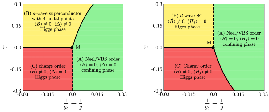
Figure 1: We are interested in a SU(2) gauge theory with $N_{f}$ fundamental Dirac fermions, and $N_{b}=2$ fundamental complex scalars. We show phase diagrams of two distinct large $N_{f}$ and $N_{b}$ limits, with $N_{f}/N_{b}$ fixed. First order phase transitions are denoted with a solid line while second order phase transitions are denoted with a dashed line. (a) Phase diagram of the theory $\mathcal{L}_{\psi}+\mathcal{L}_{B}$ in (17) and (23). There is a USp$(2N_{f})\times$USp$(N_{b})\times$U(1) global symmetry for $v\neq 0$. (b) Phase diagram in an alternative large $N_{b}$ limit discussed in Appendix A of the theory $\mathcal{L}_{\psi}+\widetilde{\mathcal{L}}_{B}$ in (17) and (129), with a USp$(2N_{f})\times$SU$(N_{b})\times$U(1) global symmetry for $v\neq 0$. The theories in (a) and (b) co-incide along the line $v=0$, when they both have USp$(2N_{f})\times$USp$(2N_{b})$ global symmetry. The two theories are also identical for the physically interesting case with $N_{f}=N_{b}=2$ for all $v$.

Our main results here are obtained by two different large flavor expansions of our SU(2) gauge theory. The resulting phase diagrams in Fig. 1 contains first-order boundaries, a multi-critical point M where all three phases meet, and second-order transitions between Néel/VBS order, charge order, and nodal $d$-wave superconductivity. The multi-critical point M and the second-order transition are described by deconfined critical SU(2) gauge theories. We will determine the scaling dimensions of gauge-invariant Néel, valence bond solid (VBS), $d$-wave superconductor, and charge order parameters in these critical theories.

Of particular interest is the scaling dimension of the gauge-invariant electron operator, which we also determine. This controls the manner in which gapless nodal quasiparticles emerge in the $d$-wave superconductor across the transition from an insulator with a non-zero gap to charged excitations. We summarize the results on scaling dimensions in Table 3. Ref. 22 considered a mean-field theory of the corresponding transition in the electron-doped cuprates: in this case, the transition is to a pseudogap-metal, but the nodal region of the Brillouin zone can be gapped in the electron-doped pseudogap metal. Thus our theory has a remarkable feature not present in BCS theory: gapless nodal quasiparticles appear in a superconductor at a momentum which is gapped in the normal state. As we noted above, Ref. 22 pointed out connections of this feature to recent photoemission experiments in the electron-doped cuprates [28].

Section II introduces the SU(2) lattice gauge theory of interest in this paper. This theory is defined in terms of fermionic spinons $f_{{\bm{i}}\alpha}$, $\alpha=\uparrow,\downarrow$ and charge $e$ bosons $B_{{\bm{i}}}$ on the sites ${\bm{i}}$ of the square lattice. Both the fermionic and bosonic matter fields transform as SU(2) gauge fundamentals, and there is also a dynamical SU(2) gauge field on the links of the lattice. We then consider the most general lattice gauge theory for these matter and gauge fields consistent with the projective symmetry transformations of the $\pi$-flux spin liquid, and with gauge-invariant observables having the same symmetry signatures as the Hubbard model with particle-hole symmetry. In the limit of strong gauge couplings, we can perform a strong-coupling expansion of our lattice gauge theory by integrating out the lattice gauge fields [23], and this will lead to the extended Hubbard model corresponding to our SU(2) lattice gauge theory. See Chapter 14 of Ref. 58 for a simpler example of a conventional theory of gauge-invariant degrees of freedom obtained from a lattice gauge theory of partons.

Note that our method is the converse of that usually followed in the condensed matter literature. We do not start from a lattice model of correlated electrons, and then obtain a gauge theory by fractionalizing the electrons. Instead, we start from a lattice gauge theory and match it to the electronic problem of interest by general arguments based on gauge invariance and global symmetry. This is a powerful method of incorporating non-perturbative knowledge of a fractionalized state (in our case, the $\pi$-flux spin liquid) in a very general setting.

Section III describes the continuum limit of the lattice gauge theory of Section II along the lines of Ref. 18. This leads to a quantum field theory of $N_{f}=2$ Dirac fermions and $N_{b}=2$ complex scalars, both transforming as SU(2) gauge fundamentals. We also discuss the generalizations of this theory to general $N_{f,b}$, and the operators corresponding to the gauge-invariant observables of the Hubbard model.

Section IV examines the nature of fermion-boson couplings in the continuum field theory without any spatial and temporal gradients. We find that there are no allowed terms which are relevant in the large $N_{f,b}$ expansion of critical theories. However, we do need to consider the higher-order formally irrelevant terms because they are important in determining the fate of the spin gap in the Higgs phases where the bosons are condensed.

Section V describes the $N_{b}=\infty$ saddle points of the continuum theories which lead to the phase diagrams in Fig. 1.

Section VI computes the $1/N_{f,b}$ corrections to the scaling dimensions of the $d$-wave superconducting, Néel, and charge order parameters, and the electron operator at momenta $(\pm\pi/2,\pm\pi/2)$. This is carried out by the SU(2) gauge theory analog of the computations in Ref. 59 for U(1) gauge theories.

II SU(2) lattice gauge theory

We begin by recalling the SU(2) lattice gauge theory of Ref. 18 in the simpler setting of a half-filled square lattice, with no Fermi surfaces in any of the states studied. We also assume a particle-hole symmetry. This lattice gauge theory is likely free of a sign problem in quantum Monte Carlo.

We write the electron spin operators as

$${C}_{{\bm{i}}}=\left(\begin{array}[]{c}{c}_{{\bm{i}}\uparrow}\\ {c}_{{\bm{i}}\downarrow}^{\dagger}\end{array}\right)\,,$$ (1)

on sites ${\bm{i}}$ of a square lattice. We fractionalize the electrons into fermionic spinons $f_{{\bm{i}}\alpha}$, $\alpha=\uparrow,\downarrow$ and charge $e$ bosons $B_{{\bm{i}}}$ via [3]

$$C_{{\bm{i}}}=\mathcal{B}_{{\bm{i}}}^{\dagger}\psi_{\bm{i}}\,,$$ (2)

where

$$\psi_{{\bm{i}}}\equiv\left(\begin{array}[]{c}f_{{\bm{i}}\uparrow}\\ f_{{\bm{i}}\downarrow}^{\dagger}\end{array}\right)\,,$$ (3)

and

$$B_{\bm{i}}\equiv\left(\begin{array}[]{c}B_{1{\bm{i}}}\\ B_{2{\bm{i}}}\end{array}\right)\quad,\quad\mathcal{B}_{\bm{i}}\equiv\left(\begin{array}[]{cc}B_{1{\bm{i}}}&-B_{2{\bm{i}}}^{\ast}\\ B_{2{\bm{i}}}&B_{1{\bm{i}}}^{\ast}\end{array}\right)\,.$$ (4)

This fractionalization introduces a SU(2) gauge symmetry, where

$$\psi_{\bm{i}}\rightarrow U_{\bm{i}}\psi_{\bm{i}}\quad,\quad B_{{\bm{i}}}\rightarrow U_{\bm{i}}B_{{\bm{i}}}\,,$$ (5)

under a SU(2) gauge transformation $U_{\bm{i}}$.

Remarkably, essentially all of the physics of the $\pi$-flux spin liquid phase, and its descendants, studied here are consequences of the SU(2) gauge symmetry, the spin rotation symmetry, and the action of other symmetries on the spinons as summarized in Table. 1.

Symmetry	$c_{\alpha}$	$f_{\alpha}$	$B_{a}$
$T_{x}$	$c_{\alpha}$	$(-1)^{y}f_{\alpha}$	$(-1)^{y}B_{a}$
$T_{y}$	$c_{\alpha}$	$f_{\alpha}$	$B_{a}$
$P_{x}$	$c_{\alpha}$	$(-1)^{x}f_{\alpha}$	$(-1)^{x}B_{a}$
$P_{y}$	$c_{\alpha}$	$(-1)^{y}f_{\alpha}$	$(-1)^{y}B_{a}$
$P_{xy}$	$c_{\alpha}$	$(-1)^{xy}f_{\alpha}$	$(-1)^{xy}B_{a}$
$\mathcal{T}$	$\varepsilon_{\alpha\beta}c_{\beta}$	$(-1)^{x+y}\varepsilon_{\alpha\beta}f_{\beta}$	$(-1)^{x+y}B_{a}$
$\mathcal{C}$	$(-1)^{x+y}\varepsilon_{\alpha\beta}c_{\beta}^{\dagger}$	$\varepsilon_{\alpha\beta}f_{\beta}^{\dagger}$	$(-1)^{x+y}B_{a}^{\ast}$

Table 1: Projective transformations of the $f_{{\bm{i}}\alpha}$ spinons and $B_{{\bm{i}}}$ chargons on lattice sites ${\bm{i}}=(x,y)$ under the symmetries $T_{x}:(x,y)\rightarrow(x+1,y)$; $T_{y}:(x,y)\rightarrow(x,y+1)$; $P_{x}:(x,y)\rightarrow(-x,y)$; $P_{y}:(x,y)\rightarrow(x,-y)$; $P_{xy}:(x,y)\rightarrow(y,x)$; time-reversal $\mathcal{T}$, and particle-hole symmetry $\mathcal{C}$. The indices $\alpha,\beta$ refer to global SU(2) spin, while the index $a=1,2$ refers to gauge SU(2). Also shown are the (non-projective) transformations of the gauge-invariant electron $c_{\alpha}$.

The action of the latter symmetries on the $B$ chargons follows from the decomposition (2), and these are also shown in Table 1. A key property of Table 1 is the relation

$$T_{x}T_{y}=-T_{y}T_{x}\,,$$ (6)

which ensures $\pi$-flux on both spinons and chargons, and at least two degenerate minima in the dispersion the chargons.

The degrees of freedom of our lattice gauge theory are one SU(2) fundamental fermion $\psi_{\bm{i}}$ on each lattice site, one SU(2) fundamental boson $B_{\bm{i}}$ on each lattice site, and a SU(2) link field $U_{{\bm{i}}{\bm{j}}}$ on each nearest-neighbor link of the square lattice. We now describe the various terms in the Hamiltonian coupling these degrees of freedom.

The simplest fermion spinon imaginary time ($\tau$) Lagrangian compatible with Table 1 is

$$\mathcal{L}(\psi)=\sum_{\bm{i}}\psi_{\bm{i}}^{\dagger}D_{\tau}\psi_{\bm{i}}^{\phantom{\dagger}}-iJ\sum_{\langle{\bm{i}}{\bm{j}}\rangle}\left[\psi_{{\bm{i}}}^{\dagger}e_{{\bm{i}}{\bm{j}}}^{\vphantom{\dagger}}U_{{\bm{i}}{\bm{j}}}^{\vphantom{\dagger}}\psi_{{\bm{j}}}^{\vphantom{\dagger}}+{\bm{i}}\leftrightarrow{\bm{j}}\right]\,,$$ (7)

where $D_{\tau}$ is a co-variant time derivative, ${\bm{i}}$,${\bm{j}}$ are nearest-neighbors, $J$ is a real coupling constant of order the antiferromagnetic exchange,

$$e_{{\bm{j}}{\bm{i}}}=-e_{{\bm{i}}{\bm{j}}}$$ (8)

is a fixed element of the $\mathbb{Z}_{2}$ center of the gauge SU(2) which ensures $\pi$ flux per plaquette; we choose

$$e_{{\bm{i}},{\bm{i}}+\hat{{\bm{x}}}}=1\,,\quad e_{{\bm{i}},{\bm{i}}+\hat{{\bm{y}}}}=(-1)^{x}\,,$$ (9)

where ${\bm{i}}=(x,y)$, $\hat{\bm{x}}=(1,0)$, $\hat{\bm{y}}=(0,1)$. The link field $U_{{\bm{i}}{\bm{j}}}=U_{{\bm{j}}{\bm{i}}}^{\dagger}$ is the fluctuating SU(2) lattice gauge field, and the mean-field saddle point of the $\pi$-flux phase is obtained by setting $U_{{\bm{i}}{\bm{j}}}=1$. The hopping term in $\mathcal{L}(\psi)$ has been chosen pure imaginary as that ensures a simple coupling to the SU(2) gauge field, along with SU(2) spin rotation invariance. The spin operator on each site ${\bm{S}}_{{\bm{i}}}=(1/2)f_{{\bm{i}}\alpha}^{\dagger}{\bm{\sigma}}_{\alpha\beta}f_{{\bm{i}}\beta}^{\vphantom{\dagger}}$ (${\bm{\sigma}}$ are the Pauli matrices) can be expressed in terms of the $\psi_{\bm{i}}$ in the following SU(2) gauge-invariant combinations:

$$2S_{z{\bm{i}}}=\psi_{\bm{i}}^{\dagger}\psi_{\bm{i}}^{\phantom{\dagger}}-1\quad,\quad S_{x{\bm{i}}}-\mathrm{i}S_{y{\bm{i}}}=-\varepsilon_{ab}\psi_{a{\bm{i}}}\psi_{b{\bm{i}}}\,,$$ (10)

where $a,b=1,2$ are SU(2) gauge indices, and $\varepsilon_{ab}$ is unit antisymmetric tensor. The nearest-neighbor bond energy operator can be identified with each individual term in $H_{f}$

$$\mbox{bond energy:~{}}\left\langle{\bm{S}}_{\bm{i}}\cdot{\bm{S}}_{\bm{j}}\right\rangle\sim Q_{f,{\bm{i}}{\bm{j}}}=Q_{f,{\bm{j}}{\bm{i}}}=-i\left[\psi_{{\bm{i}}}^{\dagger}e_{{\bm{i}}{\bm{j}}}^{\vphantom{\dagger}}U_{{\bm{i}}{\bm{j}}}^{\vphantom{\dagger}}\psi_{{\bm{j}}}^{\vphantom{\dagger}}+{\bm{i}}\leftrightarrow{\bm{j}}\right]\,.$$ (11)

In the cuprates, modulations of $Q_{f,{\bm{i}}{\bm{j}}}$ would show up as modulations in the charge density on the sites (and similarly for modulations in $Q_{b,{\bm{i}}{\bm{j}}}$ below).

Turning to the bosonic partons, and following Ref. 18, we can also write down the most general effective Lagrangian for the $B_{\bm{i}}$, keeping only terms quadratic and quartic in the $B_{\bm{i}}$, and with only on-site or nearest-neighbor couplings:

$$\mathcal{L}(B)=\sum_{\bm{i}}\left|D_{\tau}B_{\bm{i}}\right|^{2}+r\sum_{{\bm{i}}}B^{\dagger}_{{\bm{i}}}B_{{\bm{i}}}^{\vphantom{\dagger}}-iw_{1}\sum_{\langle{\bm{i}}{\bm{j}}\rangle}\left[B_{{\bm{i}}}^{\dagger}e_{{\bm{i}}{\bm{j}}}^{\vphantom{\dagger}}U_{{\bm{i}}{\bm{j}}}^{\vphantom{\dagger}}B_{{\bm{j}}}^{\vphantom{\dagger}}+{\bm{i}}\leftrightarrow{\bm{j}}\right]+\mathcal{V}(B)\,.$$ (12)

A linear time derivative term is allowed only in the absence of particle hole symmetry, and so has been omitted. The couplings $r$, $w_{1}$ are real Landau parameters, and the quartic terms are in $\mathcal{V}(B)$. These quartic terms are more conveniently expressed in terms of quadratic gauge invariant observables. By examining the transformations in Table 1, we can deduce the following correspondences between bilinears of the $B$ with those of the bilinears of the gauge-neutral electrons:

$$\mbox{site charge density:~{}}\left\langle c_{{\bm{i}}\alpha}^{\dagger}c_{{\bm{i}}\alpha}^{\vphantom{\dagger}}\right\rangle\sim\rho_{{\bm{i}}}\equiv B^{\dagger}_{\bm{i}}B_{\bm{i}}^{\vphantom{\dagger}}$$

(the correspondence between $$\rho_{\bm{i}}$$ and site charge density holds

only in the absence of particle-hole symmetry; see Section IV),

$$\mbox{bond density:~{}}\left\langle c_{{\bm{i}}\alpha}^{\dagger}c_{{\bm{j}}\alpha}^{\vphantom{\dagger}}+c_{{\bm{j}}\alpha}^{\dagger}c_{{\bm{i}}\alpha}^{\vphantom{\dagger}}\right\rangle\sim Q_{b,{\bm{i}}{\bm{j}}}=Q_{b,{\bm{j}}{\bm{i}}}\equiv\mbox{Im}\left(B^{\dagger}_{\bm{i}}e_{{\bm{i}}{\bm{j}}}^{\vphantom{\dagger}}U_{{\bm{i}}{\bm{j}}}^{\vphantom{\dagger}}B_{\bm{j}}\right),$$

$$\mbox{bond current:~{}}i\left\langle c_{{\bm{i}}\alpha}^{\dagger}c_{{\bm{j}}\alpha}^{\vphantom{\dagger}}-c_{{\bm{j}}\alpha}^{\dagger}c_{{\bm{i}}\alpha}^{\vphantom{\dagger}}\right\rangle\sim J_{{\bm{i}}{\bm{j}}}=-J_{{\bm{j}}{\bm{i}}}\equiv\mbox{Re}\left(B^{\dagger}_{\bm{i}}e_{{\bm{i}}{\bm{j}}}^{\vphantom{\dagger}}U_{{\bm{i}}{\bm{j}}}^{\vphantom{\dagger}}B_{\bm{j}}^{\vphantom{\dagger}}\right),$$

$$\mbox{pairing:~{}}\left\langle\varepsilon_{\alpha\beta}c_{i\alpha}c_{j\beta}\right\rangle\sim\Delta_{{\bm{i}}{\bm{j}}}=\Delta_{{\bm{j}}{\bm{i}}}\equiv\varepsilon_{ab}B_{a{\bm{i}}}e_{{\bm{i}}{\bm{j}}}U_{{\bm{i}}{\bm{j}}}B_{b{\bm{j}}}\,.$$ (13)

Note that the bond density observable $Q_{b,{\bm{i}}{\bm{j}}}$ of bosons above has the same symmetry signature as the bond energy $Q_{f,{\bm{i}}{\bm{j}}}$ of fermions in (11), and both are identical to the hopping terms in $\mathcal{L}(B)$ and $\mathcal{L}(\psi)$ respectively. Now we can write an expression for $\mathcal{V}(B)$ by keeping all quartic terms which involve nearest-neighbor sites:

$$\mathcal{V}(B) = \frac{u}{2}\sum_{{\bm{i}}}\rho_{{\bm{i}}}^{2}+V_{1}\sum_{{\bm{i}}}\rho_{{\bm{i}}}\left(\rho_{{\bm{i}}+\hat{\bm{x}}}+\rho_{{\bm{i}}+\hat{\bm{y}}}\right)+g\sum_{\langle{\bm{i}}{\bm{j}}\rangle}\left|\Delta_{{\bm{i}}{\bm{j}}}\right|^{2}$$ (14)

$$~{}~{}~{}+J_{1}\sum_{\langle{\bm{i}}{\bm{j}}\rangle}Q_{b,{\bm{i}}{\bm{j}}}^{2}+K_{1}\sum_{\langle{\bm{i}}{\bm{j}}\rangle}J_{{\bm{i}}{\bm{j}}}^{2}.$$

We also have the usual flux energy term of lattice gauge theory for the gauge field $U_{{\bm{i}}{\bm{j}}}$

$$\mathcal{L}(U)=-\frac{1}{g}\sum_{{\bm{i}},{\bm{j}},{\bm{k}},{\bm{l}}\in\square}\mbox{Tr}\left[U_{{\bm{i}}{\bm{j}}}U_{{\bm{j}}{\bm{k}}}U_{{\bm{k}}{\bm{l}}}U_{{\bm{l}}{\bm{i}}}\right]+\mbox{c.c.}\,,$$ (15)

along with a gauge field kinetic energy [60].

Finally, we can consider quartic terms which couple the spinons and chargons directly. From the composite operators defined above we can write down the following terms involving only nearest-neighbor sites

$$\mathcal{L}(B\psi)=\sum_{\langle{\bm{i}}{\bm{j}}\rangle}\left[\lambda_{1}\,c_{{\bm{i}}\alpha}^{\dagger}c_{{\bm{j}}\alpha}^{\phantom{\dagger}}+\lambda_{1}\,c_{{\bm{j}}\alpha}^{\dagger}c_{{\bm{i}}\alpha}^{\phantom{\dagger}}+\lambda_{2}\,Q_{b,{\bm{i}}{\bm{j}}}\,Q_{f,{\bm{i}}{\bm{j}}}\right]\,.$$ (16)

Our aim is to determine the phase diagram of the above lattice gauge theory as a function of the boson ‘mass’ tuning parameter $r$, and the various quartic boson couplings in (14). The general physics is that of a transition between Higgs and confining phases of the SU(2) gauge theory, with deconfined conformal gauge theories describing continuous transitions between the phases. When $r$ is large and positive, $B$ excitations are gapped, and we can work with the fermion-only theory in (7)—this theory is expected to confine into an insulator with either Néel or VBS order [36, 46, 45]. On the other hand, when $r$ is negative, $B$ condenses in Higgs phases, and fully quenches the SU(2) gauge field. The Higgs phases break one or more of the global symmetries, based upon the correspondence in (13).

III Quantum field theory and order parameters

Now we take the continuum limit of the lattice gauge theory action in Section II, and obtain the quantum field theory studied in the present paper. We will take the simplest case in which the boson hopping terms are only nearest-neighbor, as in (12), so there are only two valleys in the boson dispersion. This will lead to a SU(2) gauge theory with $N_{f}=2$ flavors of SU(2) fundamental Dirac fermions $\psi$, and $N_{b}=2$ flavors of SU(2) fundamental bosons $B$. As for the lattice gauge theory in Section II, almost everything follows from the symmetry transformations of the fields: the continuum limits of the transformations in Table 1 are presented in Table 2.

For the continuum limit action of the fermionic spinons, we follow the notation of Ref. [40], which follows that of earlier related works [36, 61, 39], in obtaining from (7) the fermionic Lagrangian

$$\mathcal{L}_{\psi}=i\bar{\psi}\gamma^{\mu}\left(\partial_{\mu}-iA^{\alpha}_{\mu}\sigma^{\alpha}\right)\psi,$$ (17)

where $\sigma^{\alpha}$ are the Pauli matrices, $\alpha=x,y,z$, $\gamma^{\mu}$ are $2\times 2$ Dirac matrices which act on the sublattice space, $A_{\mu}^{\alpha}$ is the SU(2) gauge field, and the $\psi$ have an additional $N_{f}=2$ valley (‘flavor’) index which is not shown. From the $\psi$ bilinears, we can make a gauge-invariant 5-component real vector, which represents the $3+2$ components of the Néel and VBS order parameters [37, 38, 36]; the Néel order is a staggered modulation of the spin in (10), while the VBS order is a modulation of the bond energy in (11). The properties of $\mathcal{L}_{\psi}$ are invariant under global SO(5)_f rotations of this vector, and all our analysis below will preserve this SO(5)_f symmetry (the $f$ subscript merely denotes that the symmetry acts on the fermions).

It is a simple matter to generalize (17) to arbitrary integer $N_{f}$: we allow the valley index to run over $1\ldots N_{f}$. After transforming to Majorana fermions, the free fermion Lagrangian has a SO$(4N_{f})$ symmetry, and modding out the gauge symmetry as in Ref. 36, we conclude that the Lagrangian $\mathcal{L}_{\psi}$ has a USp$(2N_{f})/\mathbb{Z}_{2}$ global symmetry.

In the bosonic matter sector, we express the lattice $B_{{\bm{i}}}$ bosons in terms of complex bosons $B_{as}$, with $a=1,2$ the SU(2) gauge index, and $s=1\ldots N_{b}=2$ the valley (‘flavor’) index [18]:

$$B_{a}(\bm{r})=\left\{\begin{array}[]{c}-B_{a1}e^{i\pi(x+y)/2}+B_{a2}(\sqrt{2}+1)e^{i\pi(x-y)/2},\\ \quad\mbox{$x$ even}\\ B_{a1}(\sqrt{2}+1)e^{i\pi(x+y)/2}-B_{a2}e^{i\pi(x-y)/2},\\ \quad\mbox{$x$ odd}\end{array}\right.$$ (18)

Under particle-hole symmetry $\mathcal{C}$, the transformations in Table 1 now imply that $B_{as}\rightarrow B_{as}^{\ast}$. Then (13) leads to the following gauge-invariant order parameters in the continuum limit [18]

$$d :~{}~{}\varepsilon_{ab}B_{a1}B_{b2}$$-wave superconductor

$$x :~{}~{}B_{a1}^{\ast}B_{a1}^{\phantom{\dagger}}-B_{a2}^{\ast}B_{a2}^{\phantom{\dagger}}\equiv B^{\dagger}\mu^{z}B^{\phantom{\dagger}}$$-CDW

$$y :~{}~{}B_{a1}^{\ast}B_{a2}^{\phantom{\dagger}}+B_{a2}^{\ast}B_{a1}^{\phantom{\dagger}}\equiv B^{\dagger}\mu^{x}B^{\phantom{\dagger}}$$-CDW

$$d :~{}~{}i\left(B_{a1}^{\ast}B_{a2}^{\phantom{\dagger}}-B_{a2}^{\ast}B_{a1}^{\phantom{\dagger}}\right)\equiv-B^{\dagger}\mu^{y}B^{\phantom{\dagger}}$$-density wave (19)

where $\mu$ acts on valley indices. In terms of the lattice order parameters in (13), the $d$-wave superconductor has $\Delta_{{\bm{i}},{\bm{i}}+\hat{\bm{x}}}=-\Delta_{{\bm{i}},{\bm{i}}+\hat{\bm{y}}}$, but is independent of ${\bm{i}}$. The charge density waves (CDWs) have period 2 modulations of $Q_{b,{\bm{i}}{\bm{j}}}$ and $\rho_{\bm{i}}$ (the modulations of $\rho_{\bm{i}}$ are absent when there is particle-hole symmetry, see Section IV), and are site-centered unlike the bond-centered modulations of $Q_{f,{\bm{i}}{\bm{j}}}$ in the VBS state. The $d$-density wave order is odd under time-reversal, and has a staggered pattern of electrical currents $J_{{\bm{i}}{\bm{j}}}$. Note that the CDW and $d$-density wave orders can be written as a SO(3) vector $B^{\dagger}\mu^{i}B^{\phantom{\dagger}}$, $i=x,y,z$. In combination with the complex superconducting order, the order parameters in (19) form a SO(5)_b vector, for reasons very similar to the fermions (again the $b$ subscript denotes that this SO(5) acts on the bosons). Computing the magnitude of this SO(5)_b vector, we obtain an important identity which is easily verified by explicit evaluation

$$(B^{\dagger}B)^{2}=\left(B^{\dagger}\mu^{i}B\right)^{2}+4\left|\varepsilon_{ab}B_{a1}B_{b2}\right|^{2}\,.$$ (20)

The continuum limit of the Lagrangian (12) for the bosonic sector is

$$\mathcal{L}_{B} =\left|\left(\partial_{\mu}-iA_{\mu}^{\alpha}\sigma^{\alpha}\right)B\right|^{2}+r|B|^{2}+\bar{u}|B|^{4}$$

$$+v_{1}\left(B^{\dagger}\mu^{z}B\right)^{2}+v_{1}\left(B^{\dagger}\mu^{x}B\right)^{2}$$

$$+v_{2}\left(B^{\dagger}\mu^{y}B\right)^{2}+v_{3}\left|\varepsilon_{ab}B_{a1}B_{b2}\right|^{2}\,.$$ (21)

The first three terms in $\mathcal{L}_{B}$ have the SO(5)_b global symmetry, for reasons essentially identical to those for $\mathcal{L}_{f}$. All the order parameters in (19) are degenerate in this limit. This degeneracy and the SO(5)_b symmetry are broken by the $v_{1,2,3}$ terms in (21), which are simply squares of the order parameters in (19). The identity in (19) was overlooked in Ref. [18], and has the consequence that the 5 quartic terms in (21) are not all independent—this has no material consequence to the mean-field results of Ref. [18], apart from a redundant labeling of couplings. In the Higgs phase where $B$ is condensed, one of the order parameters in (19) must be non-zero, and, in mean-field theory, the choice is determined by the relative values of $v_{1,2,3}$ [18].

The generalization of the first three terms in (21) to arbitrary integer $N_{b}$ is straightforward, but the $v_{1,2,3}$ terms in require further consideration. We limit ourselves to the case $v_{1}=v_{2}$, so that the CDW orders and the $d$-density wave orders become degenerate. Then we can write (21) as

$$\mathcal{L}_{B} =\left|\left(\partial_{\mu}-iA_{\mu}^{\alpha}\sigma^{\alpha}\right)B\right|^{2}+r|B|^{2}+\bar{u}|B|^{4}$$

$$+v_{1}\left(B^{\dagger}\mu^{i}B\right)^{2}+v_{3}\left|\varepsilon_{ab}B_{a1}B_{b2}\right|^{2}\,.$$ (22)

Next, we use the redundancy implied by (20) to set $v_{1}=0$ in (22). Then one extension of (22) to general $N_{b}$ for the bosonic flavor indices is obtained by replacing $\varepsilon_{st}$ in the $v_{3}$ term by $\mathcal{J}_{st}$ the USp($N_{b}$) invariant tensor, consisting of $N_{b}/2$ copies of $\varepsilon_{st}$ along the diagonal. (An alternative large $N_{b}$ extension in which $v_{3}$ is set to zero is discussed in Appendix A.) In this manner we obtain a Lagrangian valid for any $N_{b}$ (following conventions in Ref. [62])

$$\mathcal{L}_{B}=\left|\left(\partial_{\mu}-iA_{\mu}^{\alpha}\sigma^{\alpha}\right)B\right|^{2}+\frac{u}{2N_{b}}\,(|B_{as}|^{2}-N_{b}/g)^{2}-\frac{v}{N_{b}}\,\left|B^{T}\mathcal{J}\varepsilon B\right|^{2}\,.$$ (23)

Recall that the indices $a,b$ act on the SU(2) gauge indices, and not the flavor indices, and so do not need a large $N_{b}$ generalization. For $N_{b}=2$, the correspondence to the couplings in (21) is $u=2N_{b}\bar{u}$, $g=-u/r$, $v=-N_{b}v_{3}/4$. For general $N_{b}$, the order parameters in (19) are replaced by the SU(2) gauge-invariant operators

$$d :~{}~{}\mathcal{J}_{st}\varepsilon_{ab}B_{as}B_{bt}$$-wave superconductor

charge order $$:~{}~{}B_{as}^{\ast}T^{i}_{st}B_{at}^{\phantom{\dagger}}$$ (24)

where $T^{i}$ are generators of USp($N_{b}$) obeying

$$T^{i\dagger}=T^{i}\quad,\quad T^{iT}\mathcal{J}+\mathcal{J}T^{i}=0\,.$$ (25)

We refer to the combined and degenerate CDW and $d$-density orders simply as ‘charge order’.

We can now use standard methods to generate a large $N_{b}$ expansion of (23) at fixed $u$, $g$, and $v$. The coupling $g$ will be used to tune across the transition, while $v$ will determine the fate of Higgs phase where $B$ is condensed. The theory in (23) has a global USp($N_{b}$)$\times$U(1) symmetry, and the Higgs phase with $B$ condensed either breaks the U(1) symmetry leading to $d$-wave superconductivity, or breaks the USp($N_{b}$) symmetry leading to degenerate CDW/$d$-density wave orders.

At $v=0$, the global symmetry of (23) is enhanced to USp$(2N_{b})/\mathbb{Z}_{2}$ (as for the fermionic spinons [36]), and the superconducting and charge orders all become degenerate. The enhanced symmetry is evident in the matrix form of the bosonic fields in (4), which generalizes in the continuum to

$$\mathcal{B}_{s}=\left(\begin{array}[]{cc}B_{1s}&-B_{2s}^{\ast}\\ B_{2s}&B_{1s}^{\ast}\end{array}\right),$$ (28)

obeying the reality condition

$$\mathcal{B}_{s}=\sigma^{y}\mathcal{B}_{s}^{\ast}\sigma^{y}\,.$$ (29)

The USp$(2N_{b})$ global symmetry $U_{g}$ then acts as right multiplication $\mathcal{B}\rightarrow\mathcal{B}U_{g}$, where $U_{g}$ is a $2N_{b}\times 2N_{b}$ matrix acting on both the $s$ flavor index, and the right matrix index of (28). The condition (29) leads to the defining conditions for USp$(2N_{b})$:

$$U_{g}^{\dagger}U_{g}=1\quad,\quad U_{g}^{T}\sigma^{y}U_{g}=\sigma^{y}\,.$$ (30)

Note, also, that the SU(2) gauge symmetry in (5) acts a left multiplication $\mathcal{B}_{s}\rightarrow U\mathcal{B}_{s}$. As in the fermion case, the USp$(2N_{b})$ and gauge SU$(2)$ share a common $\mathbb{Z}_{2}$ center, and hence the global symmetry is USp$(2N_{b})/\mathbb{Z}_{2}$.

Symmetry	$B_{a}$	$X_{ab}$
$T_{x}$	$-i\mu^{x}B_{a}$	$\mu^{x}X_{ab}$
$T_{y}$	$-i\mu^{z}B_{a}$	$\mu^{z}X_{ab}$
$P_{x}$	$B_{a}$	$-i\gamma^{x}\mu^{z}X_{ab}$
$R_{\pi/2}$	$-\frac{\mu^{x}+\mu^{z}}{\sqrt{2}}B_{a}$	$e^{i\pi\gamma^{0}/4}e^{-i\pi\mu^{y}/4}X_{ab}$
$\mathcal{T}$	$B$	$\gamma^{0}\mu^{y}X^{*}$
$\mathcal{C}$	$B^{*}$	$X\sigma^{y}$
$\text{U}(1)_{c}$	$e^{i\theta}B_{a}$	$X_{ab}$
$\text{SU}(2)_{g}$	$U_{g}B$	$XU_{g}^{\dagger}$
$\text{SU}(2)_{s}$	$B$	$U_{s}X$

Table 2: We tabulate the action of the microscopic symmetries, along with the $\text{SU}(2)$ gauge transformations, on the continuum fields. To concisely express the action of $\text{SU}(2)$ spin rotation symmetry, we represent the spinon degrees of freedom in terms of a matrix of Majorana fermions $X$. The $\gamma$ matrix $\gamma^{0}$ is the labels the temporal component.

The full action of the microscopic symmetries on the continuum fields is listed in Table 2. To retain a concise representation of the $\text{SU}(2)$ spin rotation symmetry, we re-express our spinon degrees of freedom in terms of Majorana fermions. Following Ref 36, we introduce the $4\times 2$ matrix of Majorana fermions $X_{a,s;b}$. Here $a,s,b$ are the spin, valley and gauge indices, respectively. The relation between $X$ and the Dirac fermions is given by $\psi_{a,s}=i\sigma^{y}_{a,b}X_{1,s,b}$. The $\text{SU}(2)$ gauge symmetry acts as $X_{a,s;b}\rightarrow X_{a,s;c}U^{\dagger}_{cb}$ and $\text{SU}(2)$ spin rotation symmetry acts as $X_{a,s;b}\rightarrow U_{ac}X_{c,s;b}$. The action of all the symmetries apart from spin rotation symmetry lifts directly to the complex fermions, although a $\text{U}(1)$ subgroup corresponds to a uniform phase rotation $\psi\rightarrow e^{i\theta}\psi$. Both representations will be utilized here - the Majorana representation for when a complete symmetry analysis is required, and the Dirac representation for perturbative computations.

Along with the gauge-invariant fermion and boson bilinears noted above, we will also consider mixed gauge-invariant bilinears which lead to the electron operator measured in photoemission experiments. The quantum field theory yields the electron operator near the 4 nodal points ${\bm{k}}=(\pm\pi/2,\pi/2)$. The particular combination of low-energy spinons and chargons that correspond to these nodal excitations is rather complicated, as the spinor structure of the Dirac spinons must be unpacked, i.e we consider the fields $\psi_{as\alpha}$ with gauge index $a$, valley index $s$, and spinor index $\alpha$ (which microscopically corresponds to a sublattice index). Suppressing the valley index and taking the Pauli matrices $\mu^{i}$ to act on both chargon and spinon valley indices, $B_{a}^{*}\mu^{i}\psi_{a\alpha}\equiv B_{as}^{*}\mu^{i}_{st}\psi_{at\alpha}$, we have

$$C_{{\bm{k}}=(\pi/2,\pi/2)} \propto\begin{pmatrix}B_{a}^{*}i\mu^{y}\left(\psi_{a1}+\left(\sqrt{2}+1\right)\psi_{a2}\right),\\ \epsilon_{ab}B_{a}\left(\left(\sqrt{2}+1\right)\psi_{a1}-\psi_{a2}\right)\end{pmatrix}$$ (31)

$$C_{{\bm{k}}=(-\pi/2,\pi/2)} \propto\begin{pmatrix}-B_{a}^{*}i\mu^{z}\left(\left(\sqrt{2}+1\right)\psi_{a1}+\psi_{a2}\right)\\ \epsilon_{ab}B_{a}\mu^{x}\left(-\psi_{a1}+\left(\sqrt{2}+1\right)\psi_{a2}\right).\end{pmatrix}$$

As we will show, generic operators of the form $B^{*}_{as}\psi_{as^{\prime}\alpha}$ and $\epsilon_{ab}B_{as}\psi_{bs^{\prime}\alpha}$ are all renormalized in the same way at criticality, so the details of Eq. LABEL:cBpsi will not be relevant for computing the scaling dimension of the electron operator.

We will analyze the theory $\mathcal{L}_{\psi}+\mathcal{L}_{B}$ in (17) and (23) in the limit of large $N_{f}$ and $N_{b}$, with a fixed ratio $N_{f}/N_{b}$. We obtain the leading $1/N_{f,b}$ corrections to the scaling dimensions of the gauge-invariant fermion and boson bilinear order parameters, and also the electron operators in (LABEL:cBpsi). We will also obtain the corresponding properties in an alternative large $N_{b}$ limit in Appendix A.

IV Fermion-boson interactions and spin gaps

In Section III, we constructed a Lagrangian describing spinon and chargon fluctuations and their coupling to a shared $\text{SU}(2)$ gauge field. Importantly, there exist three independent quartic chargon interactions which are relevant at tree-level and must be tuned in order to reach a continuous transition. In this section, we consider symmetry-allowed interactions between the spinons and chargons. The reason for this is twofold. First, quartic interactions involving two spinons and two chargons are marginal at tree-level, and corrections to their scaling dimension are important for the behavior of the critical theory. Second, condensation of the chargons can qualitatively modify the dispersion of the spinons in the charge-ordered phase, either by producing a gap or generating a Fermi surface. Note that upon condensation of the chargons, the spinon becomes associated with the electron, and these dispersion modifications are reflected in the electronic spectral function. We show that in fact no quartic chargon-spinon interactions are allowed by the microscopic symmetries in the critical theory, provided we enforce particle-hole symmetry. Relaxing particle-hole symmetry admits two quartic interactions. In the charge ordered phase, these terms shift the Fermi energy of the Dirac spinons, thereby inducing a spinon Fermi surface.

In this section, we will use the Majorana representation of the fermionic spinons; the explicit action of spin rotation symmetry is essential in our symmetry analysis. In this language, a generic quartic interaction that respects both charge conservation and spin rotation invariance can be expressed in the form

$$\sum_{\alpha,\beta,j}A_{\alpha,\beta,j}\text{Tr}\left[B\mu^{\alpha}B^{\dagger}\overline{X}\gamma^{j}\mu^{\beta}X\right],$$ (32)

where $\bar{X}\equiv X^{\dagger}\gamma^{0}$ and $A$ is a coefficient tensor, not to be confused with the gauge field. The indices $\alpha\,,\beta\,,j$ run over four variables, the three Pauli and $\gamma$ matrices as well as an additional identity element. We perform a systematic search for symmetry-allowed quartic couplings by deducing the action of the microscopic symmetries on $A_{\alpha,\beta,j}$, which we regard as a $4^{3}=64$-dimensional vector. Symmetry-allowed quartic terms are given by choices of $A$ which have eigenvalue $1$ under all the symmetries, the existence of which can be checked numerically.

With this approach, we deduce two terms that are allowed by all the microscopic symmetries, but are odd under particle-hole symmetry which we assume to be emergent in the critical theory:

$$\text{Tr}\left[BB^{\dagger}\overline{X}\gamma^{0}X\right]\,,$$ (33)

$$\text{Tr}\left[B\mu^{z}B^{\dagger}\overline{X}\mu^{z}\gamma^{x}X\right]+\text{Tr}\left[B\mu^{x}B^{\dagger}\overline{X}\mu^{x}\gamma^{y}X\right]\,.$$

One can also consider analogous quartic couplings of the form $\sum_{\alpha,\beta,j}C_{\alpha,\beta,j}\text{Tr}\left[B\mu^{\alpha}B^{\dagger}\right]\text{Tr}\left[\overline{X}\gamma^{j}\mu^{\beta}X\right]$. The tensor $C$ transforms identically to $A$; however, the two quartic couplings in this case vanish identically due to the anticommutation relations of the Majorana fermions. These results are consistent with taking the continuum limit of the quartic spinon-chargon interactions on the lattice given by (16), where we find that the leading order terms with no derivatives vanish. Allowing for quartic interactions that break particle-hole symmetry, such as an on-site chemical potential or a second-neighbor electron hopping, generate the continuum interactions in (33). The first term acts as a chemical potential and, at each of the two gapless points in momentum space, induces an equal and opposite shift in the Fermi energy on the two species of spinons.

Quartic interactions do not generate a spin gap in the ordered phases. To find six-term interactions that can open up a spin gap in the CDW phase, we take the approach of considering the CDW order parameter, $B^{\dagger}\mu^{z}B$ and $B^{\dagger}\mu^{x}B$ for $x$-CDW and $y$-CDW respectively, and coupling them to a quartic chargon-spinon interaction that has the same symmetry transformations. Multiple six-term interactions can be obtained in this manner; however, only two are capable of producing a spin gap, which are

$$B^{\dagger}\mu^{z}B\text{Tr}\left[B\mu^{x}B^{\dagger}\overline{X}\mu^{y}X\right]\,,$$ (34)

$$B^{\dagger}\mu^{x}B\text{Tr}\left[B\mu^{z}B^{\dagger}\overline{X}\mu^{y}X\right]\,.$$

Note that these terms vanish unless both the $x$-CDW and $y$-CDW terms are non-zero. This is consistent with the fact that, once we are in the CDW phase, one is allowed to add non-gauge-invariant terms to the spinon dispersion which break translational symmetry. The symmetry transformations of gauge singlet and triplet spinon bilinears were tabulated in Ref. 61; from this analysis, one can conclude that the only possible mass term in the CDW phase, $\text{Tr}\left[\sigma^{a}\overline{X}\mu^{y}X\right]$, must be odd under translations in both the $x$ and $y$ directions. This term also breaks particle-hole symmetry; however, as it is proportional to four powers of the chargon condensate, it will generically be smaller than the previously-discussed perturbations which generate a spinon Fermi surface.

V Large $N_{b}$ saddle point

This section examines the bosonic theory $\mathcal{L}_{B}$ in (23), and determines its phase diagram at $N_{b}=\infty$. We introduce decouplings fields $\lambda$ and $\Delta$ to obtain from (23)

$$\mathcal{L}_{B}=|D_{\mu}B_{as}|^{2}+\frac{N_{b}\lambda^{2}}{2u}+\frac{N_{b}|\Delta|^{2}}{v}+\mathrm{i}\lambda(|B_{as}|^{2}-N_{b}/g)-\Delta\,\mathcal{J}_{st}\varepsilon_{ab}B^{\ast}_{as}B^{\ast}_{bt}-\Delta^{\ast}\,\mathcal{J}_{st}\varepsilon_{ab}B_{bt}B_{as}.$$ (35)

The saddle point value of $\mathrm{i}\lambda$ will determine the mass of the $B$ bosons, while $(N_{b}/v)\Delta$ is the superconducting order parameter in (24). In order to carry out the Gaussian integral over the $B$ bosons, it is convenient to define a Nambu basis for $B$. We would like the quadratic terms in $B$ which are associated with pairing to be completely off diagonal in our choice of basis and for the rest of the terms to be diagonal. We therefore use the fact that $\mathcal{J}_{st}$ is anti-symmetric to construct the Nambu basis:

$$\mathcal{B}_{m}=\begin{pmatrix}B_{1,2m-1}\\ B_{2,2m-1}\\ B^{*}_{2,2m}\\ -B^{*}_{1,2m}\end{pmatrix}$$ (36)

Here we have used $1,2$ to label the indices corresponding to the SU(2) gauge symmetry and $m=1,...,{N_{b}}/{2}$.

After integrating out the bosons, the effective action is:

$$S_{\text{eff.}}=\frac{N_{b}}{2}\text{Tr}\left[\text{ln}(\mathcal{G}^{-1})\right]+\frac{N_{b}\lambda^{2}}{2u}+\frac{N_{b}|\Delta|^{2}}{v}-\mathrm{i}\lambda\frac{N_{b}}{g},$$ (37)

where

$$\mathcal{G}^{-1}=\begin{pmatrix}\mathrm{i}\lambda-(\partial_{\mu}+\mathrm{i}A_{\mu}^{j}\sigma_{j})^{2}&-2\Delta\\ -2\Delta^{*}&\mathrm{i}\lambda-(\partial_{\mu}+\mathrm{i}A_{\mu}^{j}\sigma_{j})^{2}\end{pmatrix}$$ (38)

is a $4\times 4$ matrix. We assume $A_{\mu}^{j}=0$ at the saddle point (preserving gauge and Lorentz symmetry). The saddle point equation for $\lambda$ is

$$\frac{\mathrm{i}\lambda N_{b}}{u}+\frac{N_{b}}{g}=\int\frac{d^{3}p}{(2\pi)^{3}}\left(\mathrm{i}\lambda+p^{2}\right)\frac{2N_{b}}{(\mathrm{i}\lambda+p^{2})^{2}-4|\Delta|^{2}}\,,$$ (39)

and that for $\Delta$ is

$$\frac{N_{b}}{v}=\int\frac{d^{3}p}{(2\pi)^{3}}\frac{4N_{b}}{(\mathrm{i}\lambda+p^{2})^{2}-4|\Delta|^{2}}\,.$$ (40)

At the saddle point where $\Delta=0$, setting $\bar{\lambda}\equiv\mathrm{i}\lambda$ we recover the result of Ref. 59.

$$\int\frac{d^{3}p}{(2\pi)^{3}}\frac{1}{(\bar{\lambda}+p^{2})}=\frac{\bar{\lambda}}{2u}+\frac{1}{2g}\,.$$ (41)

In what follows, we will always assume $g>0$.

V.1 Solving saddle point equations

In integrating out the $B$ bosons, we have assumed there is no condensate in $B$. We will first solve the saddle point equations under the assumption that $\langle B\rangle=0$ and then consider alternate solutions where $B$ condenses. Under this assumption, the saddle point equations for $\Delta$ and $\overline{\lambda}\equiv\mathrm{i}\lambda$ obtained from integrating (40) and (39) are:

$$\frac{1}{v}=\frac{1}{4\pi}\frac{1}{|\Delta|}\left[\sqrt{\overline{\lambda}+2|\Delta|}-\sqrt{\overline{\lambda}-2|\Delta|}\right]\,,$$ (42)

$$\frac{\overline{\lambda}}{u}+\frac{1}{g}=-\frac{1}{4\pi}\left[\sqrt{\overline{\lambda}+2|\Delta|}+\sqrt{\overline{\lambda}-2|\Delta|}-\frac{4\pi}{g_{c}}\right]\,,$$ (43)

where $1/g_{c}=\Lambda/\pi^{2}$, with $\Lambda$ the momentum space cutoff. We first note the existence of a solution where $\Delta=0$ and $\overline{\lambda}$ is condensed obtained by neglecting (40), setting $\Delta=0$ in (43), and solving (43) for $\overline{\lambda}$. Such a solution is shown in Fig. 2.

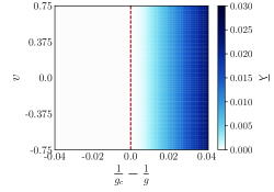
Figure 2: We show the saddle point solutions for $\overline{\lambda}$ as a function of $\frac{1}{g_{c}}-\frac{1}{g}$ and $v$ for $u=1.5$ for the solution where only $\overline{\lambda}$ is condensed and $B$ and $\Delta$ are both zero. Such a solution only exists when $g>g_{c}$ and we note the value of $\overline{\lambda}$ has no dependence on $v$ when $\langle\Delta\rangle=0$. The boundary after which $\overline{\lambda}$ is nonzero is denoted with a dotted red line.

We can also find solutions of Eq. 42 and Eq. 43 where $\lambda$ and $\Delta$ are both condensed. Multiplying the saddle point equation for $\overline{\lambda}$ and $\Delta$ together yields a constraint on $\overline{\lambda}$ which is independent of $\Delta$:

$$\overline{\lambda}=u\left(\frac{1}{g_{c}}-\frac{1}{g}-\frac{v}{4\pi^{2}}\right)$$ (44)

We then only need to assume the above relation for $\overline{\lambda}$, substitute this expression into Eq. 42 or Eq. 43, and solve for $\Delta$. The resulting solution is shown in Fig. 3, and exists only on a narrow strip for positive $v$ and $\frac{1}{g_{c}}-\frac{1}{g}$. On the lower boundary of this strip of solution, we have $\overline{\lambda}\rightarrow 2|\Delta|$.

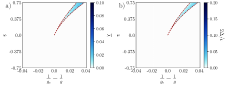
Figure 3: We show the saddle point solutions for $\overline{\lambda}$ (a) and $\Delta$ (b) for the class of solution where $\Delta$ and $\overline{\lambda}$ are both nonzero but $B$ is assumed to not be condensed as a function of $v$ and $\frac{1}{g_{c}}-\frac{1}{g}$. A real, positive solution for $\overline{\lambda}$ and $|\Delta|$ only exists for the narrow strip shown in the region where $g>g_{c}$ and $v>0$. On the lower curve of the region of existence of this solution we have $\overline{\lambda}=2|\Delta|$. The boundary enclosing the region where each quantity becomes nonzero is denoted with a dotted red line.

We now investigate a third class of solution, one where we allow $B$ to condense in addition to $\overline{\lambda}$ and $\Delta$ by allowing for a condensate in the $m=1$ component of (36)

$$\left\langle\mathcal{B}_{m}\right\rangle=\sqrt{N_{b}}\begin{pmatrix}B_{1,1}\\ B_{2,1}\\ B^{*}_{2,2}\\ -B^{*}_{1,2}\end{pmatrix}\delta_{m1}\,.$$ (45)

After integrating out the $m>1$ components, we obtain the large $N_{b}$ effective action generalizing (37)

$$S_{\text{eff.}}= \frac{N_{b}}{2}\text{Tr}\left[\text{ln}(\mathcal{G}^{-1})\right]-\frac{N_{b}\overline{\lambda}^{2}}{2u}+\frac{N_{b}|\Delta|^{2}}{v}-\overline{\lambda}\frac{N_{b}}{g}$$

$$+N_{b}\left[\overline{\lambda}(|B_{a1}|^{2}+|B_{a2}|^{2})-\Delta B^{*}_{as}B^{*}_{bt}\varepsilon_{ab}\varepsilon_{st}-\Delta^{*}B_{as}B_{bt}\varepsilon_{ab}\varepsilon_{st}\right]\,.$$ (46)

The saddle point equations for $B$ are:

$$\overline{\lambda}B^{*}_{1,1}-2\Delta^{*}B_{2,2}=0\qquad\overline{\lambda}B^{*}_{2,1}+2\Delta^{*}B_{1,2}=0\qquad\overline{\lambda}B^{*}_{1,2}+2\Delta^{*}B_{2,1}=0\qquad\overline{\lambda}B^{*}_{2,2}-2\Delta^{*}B_{1,1}=0\,.$$ (47)

We note that combining the above equations produces the constraint:

$$\overline{\lambda}=2|\Delta|\,.$$ (48)

Additionally, we note that the saddle point equations for $B$ imply that if $\overline{\lambda}$, $\Delta$, and $B$ all condense, the $d$-wave order parameter in (19) also must condense. The saddle point equation for $\overline{\lambda}$ becomes:

$$\frac{2|\Delta|}{u}+\frac{1}{g}-\frac{1}{g_{c}}-(|B_{a,1}|^{2}+|B_{a,2}|^{2})=-\frac{\sqrt{|\Delta|}}{2\pi}\,,$$ (49)

while the saddle point equation for $\Delta$ when $B$ is nonzero becomes:

$$\frac{1}{v}-\frac{1}{|\Delta|}(|B_{a,1}|^{2}+|B_{a,2}|^{2})=\frac{1}{2\pi\sqrt{|\Delta}|}\,.$$ (50)

Combining the two equations yields:

$$|B_{a,1}|^{2}+|B_{a,2}|^{2}=-\frac{\sqrt{|\Delta|}}{2\pi}+\frac{|\Delta|}{v}\implies|\Delta|\left(\frac{1}{2v}-\frac{1}{u}\right)-\frac{\sqrt{|\Delta|}}{2\pi}+\frac{1}{2}\left(\frac{1}{g_{c}}-\frac{1}{g}\right)=0\,,$$ (51)

such that we have solutions corresponding to $\sqrt{|\Delta|}$:

$$\sqrt{|\Delta|}=\frac{\frac{1}{2\pi}\pm\sqrt{\left(\frac{1}{2\pi}\right)^{2}-2\left(\frac{1}{2v}-\frac{1}{u}\right)\left(\frac{1}{g_{c}}-\frac{1}{g}\right)}}{2\left(\frac{1}{2v}-\frac{1}{u}\right)}$$ (52)

The two branches for which $\sqrt{|\Delta|}$ is real and positive are shown in Fig. 5 and Fig. 4.

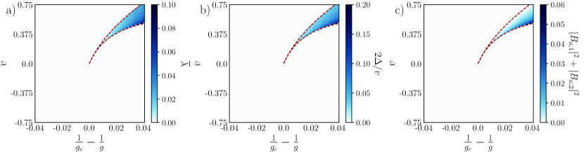
Figure 4: We show the saddle point solutions for $\overline{\lambda}$ (a), $\Delta$ (b), and $B$ (c) for the class of solution where all are allowed condensed for a the first branch of the solution corresponding to Eq. 52 as a function of $\frac{1}{g_{c}}-\frac{1}{g}$ and $v$ for $u=1.5$. The boundary enclosing the region where each quantity becomes nonzero is denoted with a dotted red line. We note that a solution with a positive and real $\sqrt{|\Delta|}$ only exists for $v>0$ and $g>g_{c}$. The upper boundary of this solution aligns with the lower boundary of the solution in Fig. 3.

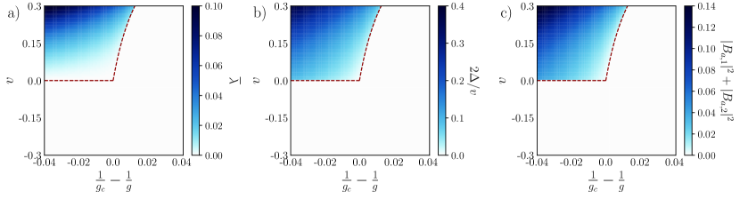
Figure 5: We show the saddle point solutions for $\overline{\lambda}$ (a), $\Delta$ (b), and $B$ (c) for the class of solution where all are allowed condensed for a the second branch of the solution corresponding to Eq. 52 as a function of $\frac{1}{g_{c}}-\frac{1}{g}$ and $v$ for $u=1.5$. This class of solution exists only when $v>0$ and unlike the solution corresponding to the first branch of Eq. 52 plotted in Fig. 4, the solution corresponding to to second branch exists when $0<g<g_{c}$. We note the difference in scale of the magnitude of the plotted quantities as compared to Fig. 4 for the same range of $v$. The boundary enclosing the region where each quantity becomes nonzero is denoted with a dotted red line.

The first order phase boundary between phases A and B is determined by where the argument of the square root in (52) becomes negative and lies along the curve:

$$v=\left({1}/{g_{c}}-{1}/{g}\right)\left[(2\pi)^{-2}+({2}/{u})({1}/{g_{c}}-{1}/{g})\right]^{-1}\,.$$ (53)

Finally, there is a final type of possible solution where only $B$ is condensed, and $\langle\overline{\lambda}\rangle=\langle\Delta\rangle=0$. Such a solution must obey $|B_{1}|^{2}+|B_{2}|^{2}=-\frac{1}{g_{c}}+\frac{1}{g}$, but unlike the solution where $\Delta$ and $\overline{\lambda}$ are also condensed, there is no constraint from the saddle point equations to determine which order parameters in (19) are nonzero when $\langle B\rangle\neq 0$. We argue that the order parameter which condenses can be determined from the sign of $v$ from the original action in (23) by noting that when $v$ is positive, it is energetically favorable for the superconducting order parameter in the $B$’s to become nonzero while if $v$ is negative, it is favorable for the $d$-density wave or CDW to become nonzero.

We have presented four possible classes of solutions; a solution where only $B$ is condensed, a solution where only $\overline{\lambda}$ is condensed, a solution where $\overline{\lambda}$ and $\Delta$ are condensed but $\langle B\rangle=0$, and a solution where $\overline{\lambda}$, $\Delta$, and $B$ all condense. The phase diagram is then determined by plugging each solution into (V.1) and choosing the one with the lowest free energy. After integration, (V.1) becomes:

$$\begin{split}\frac{S_{\text{eff.}}}{N_{b}}=&-\frac{1}{6\pi}\left[\left(\overline{\lambda}+2|\Delta|\right)^{3/2}+\left(\overline{\lambda}-2|\Delta|\right)^{3/2}\right]+\frac{2}{3\pi^{2}}\Lambda\overline{\lambda}-\frac{2}{9\pi^{2}}\Lambda^{3}+\frac{1}{6\pi^{2}}\Lambda^{3}\text{ln}\left[(\overline{\lambda}+\Lambda^{2})^{2}-4|\Delta|^{2}\right]-\frac{\overline{\lambda}^{2}}{2u}\\ &+\frac{|\Delta|^{2}}{v}-\frac{\overline{\lambda}}{g}+\overline{\lambda}(|B_{a1}|^{2}+|B_{a2}|^{2})-\Delta B^{*}_{as}B^{*}_{bt}\varepsilon_{ab}\varepsilon_{st}-\Delta^{*}B_{as}B_{bt}\varepsilon_{ab}\varepsilon_{st}\,.\end{split}$$ (54)

In practice we compute the above with a cutoff $\Lambda=100$, and find the low energy phases shown in Fig. 6. We note that when $B$ is condensed such that $\overline{\lambda}=2|\Delta|$, there is no direct dependence of the effective action on $B$ in the above.

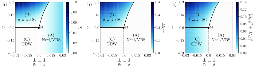
Figure 6: We show the lowest energy saddle point solutions for $\overline{\lambda}$ (a), $|\Delta|$ (b), and $|B_{a,1}|^{2}+|B_{a,2}|^{2}$ and (c) as a function of $\frac{1}{g_{c}}-\frac{1}{g}$ and $v$. We denote the boundaries between each phase with a black solid line if the phase boundary is first order and a black dotted line if the phase boundary is second order. The lowest energy solution for $g>g_{c}$ is the solution plotted in Fig. 2 with only $\langle\overline{\lambda}\rangle\neq 0$ in the region where the solution shown in Fig. 5 (the one where $\Delta$, $B$, and $\overline{\lambda}$ are all condensed) does not exist; this solution corresponds to either Neel or VBS order since neither $\Delta$ nor $B$ are condensed. In the region where $v>0$ where the solution shown in Fig. 5 does exist, it is always the lowest energy solution; this solution corresponds to a $d$-wave superconductor. For $0<g<g_{c}$ and $v<0$, the only possible solution is the one where only $B$ is condensed; based off our arguments in the text, since this solution is the lowest energy only for $v<0$, such a solution corresponds to charge order.

VI Computations at order $1/N_{f,b}$

For convenience, we present the complete Lagrangian $\mathcal{L}=\mathcal{L}_{\psi}+\mathcal{L}_{B}$ in (17) and (35) for our SU(2) gauge theory.

$$\mathcal{L}=i\bar{\psi}\not{D}_{\mu}\psi+|D_{\mu}B_{as}|^{2}+\frac{N_{b}\lambda^{2}}{2u}+\frac{N_{b}|\Delta|^{2}}{v}+\mathrm{i}\lambda(|B_{as}|^{2}-N_{b}/g)-\mathcal{J}_{st}\varepsilon_{ab}(\Delta B_{as}^{*}B_{bt}^{*}+\Delta^{*}B_{bt}B_{as}).$$ (55)

The kinetic term for boson should be understood as

$$|(D_{\mu}B_{s})_{a}|^{2}\equiv(\partial_{\mu}B_{a}^{*}-\mathrm{i}B_{b}^{*}\sigma^{j}_{ba}A_{j})(\partial_{\mu}B_{a}+\mathrm{i}A_{j}\sigma_{ab}^{j}B_{b}).$$ (56)

We will study (55) in a large $N_{f,b}$ expansion, with $N_{f}/N_{b}$ fixed. This is similar to the method followed in Ref. 59 for a U(1) gauge theory.

VI.1 Multicritical point at $v=0$

First we consider the multicritical point M in Fig. 1, where we can ignore the pairing field $\Delta$ in (55), and work with a Lagrangian with $\text{USp}(2N_{f})\times\text{USp}(2N_{b})/\mathbb{Z}_{2}$ global symmetry:

$$\mathcal{L}_{0}=\mathrm{i}\bar{\psi}\not{D}_{\mu}\psi+|D_{\mu}B_{as}|^{2}+\frac{N_{b}\lambda^{2}}{2u}+\mathrm{i}\lambda(|B_{as}|^{2}-N_{b}/g)\,.$$ (57)

Taking the Fourier transformation and integrating over the bosons and fermions, we write the free energy as

$${\mathcal{F}}_{0}=\text{Tr}\ln\mathcal{G}^{-1}_{b}+N_{b}\left(\frac{\lambda^{2}}{2u}-\frac{\lambda}{g}\right)+\text{Tr}\ln\mathcal{G}^{-1}_{f},$$ (58)

where $\mathcal{G}^{-1}_{b}$ is a $2N_{b}\times 2N_{b}$ matrix of block-diagonal form $\mathcal{G}^{-1}_{b}=\left(\begin{matrix}\mathcal{G}^{-1}_{A}&0\\ 0&\mathcal{G}^{-1}_{D}\end{matrix}\right)$ in the Nambu basis:

$$\mathcal{G}^{-1}_{A/D}=\mathbbm{1}\left[\delta_{kk^{\prime}}k^{2}+\mathrm{i}\lambda(k-k^{\prime})+\int\frac{d^{3}q}{(2\pi)^{3}}A_{\alpha}(q)A^{\alpha}(k-k^{\prime}-q)\right]\pm\sigma^{\alpha}\left[(k+k^{\prime})_{\mu}A_{\alpha}^{\mu}(k-k^{\prime})\right].$$ (59)

$\mathcal{G}^{-1}_{f}$ is the corresponding matrix for the fermionic sector

$$\mathcal{G}^{-1}_{f}=\gamma^{\mu}[-\delta_{kk^{\prime}}k_{\mu}\mathbbm{1}+A_{\mu}^{\alpha}(k^{\prime}-k)\sigma^{\alpha}].$$ (60)

Next we expand near the saddle point by defining the propagator

$$G_{B}(k)=\frac{1}{k^{2}+\bar{\lambda}},\quad G_{\psi}=\frac{\not{k}}{k^{2}},$$ (61)

where $\bar{\lambda}=\mathrm{i}\lambda_{c}$ is real and positive. We expand the matrix log to second order, see appendix B for details. The leading correction to the free energy can be computed as

$${\mathcal{F}_{0}^{(1)}}=\frac{1}{2}\int\frac{d^{3}p}{(2\pi)^{3}}\Bigg{\{}\Pi_{\lambda}(p)\lambda(p)\lambda(-p)+A_{\alpha}^{\mu}(p)\left(\delta_{\mu\nu}-\frac{p_{\mu}p_{\nu}}{p^{2}}\right)\Pi_{A}(p)A^{\alpha}_{\nu}(-p)\Bigg{\}}+N_{b}\left(\frac{\lambda^{2}}{2u}-\frac{\lambda}{g}\right),$$ (62)

where the kernels are

$$\begin{split}&\Pi_{\lambda}(p)=\frac{2N_{b}}{4\pi p}\arctan\frac{p}{2\sqrt{\bar{\lambda}}},\\ &\Pi_{A}(p)=2N_{b}\left(\frac{4\bar{\lambda}+p^{2}}{8p\pi}\arctan\frac{p}{2\sqrt{\bar{\lambda}}}-\frac{\sqrt{\bar{\lambda}}}{4\pi}\right)+N_{f}\frac{p}{16}.\end{split}$$ (63)

The dressed propagators can also be read off,

$$\begin{split}D^{ij}_{A,\mu\nu}=\frac{\delta_{ij}}{\Pi_{A}}\left(\delta_{\mu\nu}-\zeta\frac{p_{\mu}p_{\nu}}{p^{2}}\right),\quad D_{\lambda}=\frac{1}{\Pi_{\lambda}}.\end{split}$$ (64)

Here $i,j$ are the gauge indices and $\mu,\nu$ are the spacetime indices. For simplicity we introduce the standard notation $(A_{\mu})_{aa^{\prime}}\equiv\sum_{i}A_{\mu}^{i}(\sigma^{i})_{aa^{\prime}}.$ The propagators then become

$$\langle(A_{\mu})_{ab}(A_{\nu})_{a^{\prime}b^{\prime}}\rangle(q)=(2\delta_{ab^{\prime}}\delta_{ba^{\prime}}-\delta_{aa^{\prime}}\delta_{bb^{\prime}})D_{\mu\nu}(q)=\frac{2\delta_{ab^{\prime}}\delta_{ba^{\prime}}-\delta_{aa^{\prime}}\delta_{bb^{\prime}}}{\Pi_{A}(q)}\left(\delta_{\mu\nu}-\zeta\frac{q_{\mu}q_{\nu}}{q^{2}}\right),$$ (65)

Notice that at the critical point, the kernels reduce to

$$\Pi_{\lambda}\rightarrow\frac{2N_{b}}{8p},\quad\Pi_{A,\mu\nu}\rightarrow(2N_{b}+N_{f})\frac{p}{16}.$$ (66)

VI.1.1 Dressed boson field

The anomalous dimension of the $B$ field is

$$\text{dim}[B_{as}]=\frac{3-2+\eta_{B}}{2}=\frac{1}{2}+\frac{\eta_{B}}{2},$$ (67)

where $a$ is the gauge index, and $s$ is the flavor index as usual. The operator is not gauge-invariant on its own. The corrections come from the gauge fields and $\lambda$. We draw the corresponding diagrams in 12.

Figure 7: Correction to boson propagators at $v=0$.

Since the boson propagator is the same for any flavor $(a,s)$, we can first compute the integral and then take care of the indices. The integral corresponding to fig. 7(a) is

$$\begin{split}I_{A;1}=&\int\frac{d^{3}p}{8\pi^{3}}\left[G_{B}(k+p)D_{\mu\nu}(-p)(2k+p)_{\mu}(2k+p)_{\nu}\right]\mid_{\bar{\lambda}=0}\\ \rightarrow\ &-\frac{4}{(2N_{b}+N_{f})\pi^{2}}\left(\frac{10}{3}+2\zeta\right)k^{2}\log k,\end{split}$$ (68)

where the right arrow means we are extracting the $k^{2}\log k$ divergence. Computational details for all the integrals can be found in appendix B. Taking care of the trace over internal gauge indices,

$$\sum_{a^{\prime},a^{\prime\prime}}\sigma^{j}_{aa^{\prime}}\sigma^{j}_{a^{\prime}a^{\prime\prime}}=\sum_{a^{\prime},a^{\prime\prime}}(2\delta_{aa^{\prime\prime}}-\delta_{a^{\prime}a}\delta_{a^{\prime\prime}a})=3.$$ (69)

The integral for diagram 7(b) is

$$I_{\lambda;1}=\mathrm{i}^{2}\int\frac{d^{3}p}{8\pi^{3}}\left[G_{B}(k+p)D_{\lambda}(-p)\right]\big{|}_{\bar{\lambda}=0}\rightarrow\frac{2}{3N_{b}\pi^{2}}k^{2}\log k.$$ (70)

Summing everything up, we have

$$\eta_{B}=\frac{2}{3N_{b}\pi^{2}}-\frac{12}{(2N_{b}+N_{f})\pi^{2}}\left(\frac{10}{3}+2\zeta\right).$$ (71)

VI.1.2 Charge order parameter

Next we work out the vertex corrections to get the

$$\text{dim}[B^{\dagger}_{as}T^{\alpha}_{st}B_{at}]=2\ \text{dim}[B]+\eta_{\text{vertex}},$$ (72)

where $T^{\alpha}$ is some generator of the USp$(N_{b})$ group that satisfies (25). Again we will first do the integrals and then take into account the indices. The relevant diagrams are shown in figure 13.

Figure 8: Diagrams contributing to the vertex correction of the density wave scaling dimension at leading order.

The following integral will contribute to panel (a):

$$I_{A;2}=\int\frac{d^{3}p}{8\pi^{3}}G_{B}(k_{1}-p)G_{B}(k_{2}-p)(2k_{1}-p)_{\mu}(2k_{2}-p)_{\nu}\frac{1}{\Pi_{A,\mu\nu}(p)}\left(\delta_{\mu\nu}-\zeta\frac{p_{\mu}p_{\nu}}{p^{2}}\right)$$ (73)

To extract the divergence, we can simplify the calculation by choosing $k_{1}=k_{2}.$ The expression above then gives (more details are presented in appendix B)

$$I_{A;2}\rightarrow-\frac{8}{(2N_{b}+N_{f})\pi^{2}}(1-\zeta)\log k.$$ (74)

Comparing with the tree level diagrams, there is an additional prefactor $3$ coming from the trace over gauge indices

$$\sum_{j}\sum_{a}\sigma^{j}_{a^{\prime\prime}a}\sigma^{j}_{aa^{\prime}}=3\delta_{a^{\prime}a^{\prime\prime}}.$$ (75)

Another useful integral that contributes to panel (b) is,

$$I_{\lambda;2}=\mathrm{i}^{2}\int\frac{d^{3}p}{8\pi^{3}}G_{B}(k_{1}-p)G_{B}(-k_{2}+p)D_{\lambda}(p)\rightarrow\frac{2}{N_{b}\pi^{2}}\log k,$$ (76)

where we again have imposed $k_{1}=k_{2}$ and extracted the term proportional to $\log k$. Combining the contributions, we get

$$\eta_{\text{vertex}}=\frac{2}{N_{b}\pi^{2}}-\frac{8\cdot 3}{(2N_{b}+N_{f})\pi^{2}}(1-\zeta).$$ (77)

The dimension of the quadratic boson term is thus,

$$\text{dim}[B^{\dagger}_{as}T^{\alpha}_{st}B_{at}]=(1+\eta_{B})+\eta_{\text{vertex}}=1+\frac{8}{3(2N_{b}+N_{f})\pi^{2}}\left(\frac{N_{f}}{N_{b}}-22\right).$$ (78)

At $N_{f}=N_{b}=2,$ we have above equal to $1-28/3\pi^{2}=0.054$. Our anomalous scaling dimension is

$$\eta_{B^{2}}=1+2\eta_{B}+2\eta_{\text{vertex}}=1+\frac{16}{3(2N_{b}+N_{f})\pi^{2}}\left(\frac{N_{f}}{N_{b}}-22\right).$$ (79)

VI.1.3 Superconducting order parameter

Next we work out the vertex corrections to get the

$$\text{dim}\left[B_{as}\varepsilon_{ab}\mathcal{J}_{st}B_{bt}\right]=2\ \text{dim}[B]+\iota_{\text{vertex}}.$$ (80)

At $v=0$, the result is guaranteed by symmetry to be the same as that of the charge order computed in the previous section, but we still present it here for completeness. The relevant diagrams are shown in 9. We will again first compute the integrals and then take into account the indices.

Figure 9: Vertex corrections to the superconducting order parameter.

The useful integral in panel (a) is

$$\begin{split}I_{A;3}=&\int\frac{d^{3}p}{8\pi^{3}}G_{B}(k_{1}-p)G_{B}(-k_{2}+p)(2k_{1}-p)_{\mu}(-2k_{2}+p)_{\nu}\frac{1}{\Pi_{A,\mu\nu}(p)}\left(\delta_{\mu\nu}-\zeta\frac{p_{\mu}p_{\nu}}{p^{2}}\right)\\ \rightarrow\ &\frac{8}{(2N_{b}+N_{f})\pi^{2}}(1-\zeta)\log k.\end{split}$$ (81)

Notice the integral is different from that in (73) and the result has opposite sign. Compared with the tree level, we just have an additional factor $-3$ coming from the gauge indices

$$\sum_{a,b}\sigma^{j}_{a^{\prime}a}\varepsilon_{ab}(\sigma^{j})^{T}_{bb^{\prime}}=-3\ \varepsilon_{a^{\prime}b^{\prime}}.$$ (82)

The two minus signs therefore cancel each other and we have the same result as in the charge density wave case.

The integral relevant to panel (b) turns out to be have the same result same as that in (76),

$$I_{\lambda;3}=\mathrm{i}^{2}\int\frac{d^{3}p}{8\pi^{3}}G_{B}(k_{1}-p)G_{B}(-k_{2}+p)D_{\lambda}(p)\\ =I_{\lambda;2},$$ (83)

with no additional prefactors compared with the tree level result. Combining all contributions, we get

$$\iota_{\text{vertex}}=\frac{2}{N_{b}\pi^{2}}-\frac{8\cdot 3}{(2N_{b}+N_{f})\pi^{2}}(1-\zeta),$$ (84)

which is not surprisingly the same as that found in (71). The dimension of the pairing term is then

$$\text{dim}[B_{as}\varepsilon_{ab}\mathcal{J}_{st}B_{bt}]=1+\frac{8}{3(2N_{b}+N_{f})\pi^{2}}\left(\frac{N_{f}}{N_{b}}-22\right).$$ (85)

Our anomalous scaling dimension is again

$$\iota_{B^{2}}=1+2\eta_{B}+2\iota_{\text{vertex}}=1+\frac{16}{3(2N_{b}+N_{f})\pi^{2}}\left(\frac{N_{f}}{N_{b}}-22\right).$$ (86)

VI.1.4 Correlation length exponent

We compute the correlation length exponent $\nu$ of the order parameters,

$$\xi\propto(g-g_{c})^{-\nu}\,$$ (87)

following the method of Ref. 59. As the correlation length is gauge-invariant, the calculation can be performed in a fixed gauge and $\nu=\nu_{B}$. We will use the relation

$$\nu_{B}=\frac{\gamma_{B}}{2-\eta_{B}},$$ (88)

where the anomalous scaling dimension of single boson $\eta_{B}$ has been computed in (71), and $\gamma_{B}$ is defined as

$$G_{B}^{-1}(k=0)=(g-g_{c})^{\gamma_{B}}.$$ (89)

We will calculate $\gamma_{B}$ below. We start by defining a convenient parameter $\lambda_{g}$ to measure the deviation from the critical point, satisfying

$$\frac{1}{g_{c}}-\frac{1}{g}=\frac{\sqrt{\lambda_{g}}}{4\pi}\,.$$ (90)

To leading order, it is related to $\bar{\lambda}$ by

$$\bar{\lambda}=\lambda_{g}+\frac{\Pi_{\lambda}(k=0,\bar{\lambda}=0)}{\Pi_{\lambda}(0,\bar{\lambda})}\Sigma(0,0)\,,$$ (91)

where $\Sigma$ is the boson self energy, and its second argument refers to the mass in the boson propagator. The boson propagator can then be written as

$$G_{B}^{-1}(0)=\bar{\lambda}-\Sigma(0,\bar{\lambda})=\lambda_{g}-\left(\Sigma(0,\lambda_{g})-\frac{\Pi_{\lambda}(0,0)}{\Pi_{\lambda}(0,\lambda_{g})}\Sigma(0,0)\right)\,,$$ (92)

where second argument of $\Pi_{\lambda}$ also refers to the boson mass. In the following we will evaluate the $\lambda_{g}\log\lambda_{g}$ divergence of the self-energy diagrams appearing in (92).

Figure 10: Feymann diagrams that contribute to the (92). Gauge and flavor indices are supressed.

The relevant diagrams are shown in fig. 10, we list their contributions below:

$$\begin{split}&\Sigma^{(a)}=3I_{A;1},\\ &\Sigma^{(b)}=3\sum_{\mu,\nu}\int\frac{d^{3}p}{8\pi^{3}}\left(\delta_{\mu,\nu}-\zeta\frac{p_{\mu}p_{\nu}}{p^{2}}\right)\frac{1}{\Pi_{A}(p)},\\ &\Sigma^{(c)}=I_{\lambda;1},\\ &\Sigma^{(d)}=\frac{3\mathrm{i}^{2}}{\Pi_{\lambda}(0,\bar{\lambda})}\int\frac{d^{3}p}{8\pi^{3}}I_{A;1}(p)\big{(}G_{B}(p)\big{)}^{2}\\ &\Sigma^{(e)}=\frac{\mathrm{i}^{2}}{\Pi_{\lambda}(0,\bar{\lambda})}\int\frac{d^{3}p}{8\pi^{3}}I_{\lambda;1}(p)\big{(}G_{B}(p)\big{)}^{2}\\ &\Sigma^{(f)}=\frac{\mathrm{i}^{2}}{\Pi_{\lambda}(0,\bar{\lambda})}\Sigma^{(b)}\int\frac{d^{3}p}{8\pi^{3}}\big{(}G_{B}(p)\big{)}^{2}=-\Sigma^{(b)}.\\ \end{split}$$ (93)

where $I_{A;1}$ and $I_{\lambda;1}$ have been defined in the first equalities of the equations (68) and (70), respectively. Since $(b)$ and $(f)$ cancel each other, we just need to extract the divergence in $(a)(c)(d)(e)$. The gauge field contributions $\Sigma^{(a)}+\Sigma^{(d)}$ give:

$$\Sigma^{(a)}+\Sigma^{(d)}\rightarrow-\frac{12}{\pi^{2}}\left(\frac{7N_{f}-18N_{b}}{(2N_{b}+N_{f})^{2}}+\frac{\zeta}{2N_{b}+N_{f}}\right)\lambda_{g}\log\lambda_{g}.$$ (94)

The remaining term to be evaluated is $\Sigma^{(c)}+\Sigma^{(e)}$,

$$\Sigma^{(c)}+\Sigma^{(e)}\rightarrow\frac{3}{\pi^{2}N_{b}}\lambda_{g}\log\lambda_{g}.$$ (95)

Since the integrals are in parallel to those discussed in ref. [59], we will omit the details here. Combining the two equations above, we have the total coefficient $\alpha$ in front of the $\lambda_{g}\log\lambda_{g}$ divergence as

$$\alpha=\frac{3}{N_{b}\pi^{2}}-\frac{12}{\pi^{2}}\left(\frac{7N_{f}-18N_{b}}{(N_{f}+2N_{b})^{2}}+\frac{\zeta}{N_{f}+2N_{b}}\right).$$ (96)

Then we re-exponentiate the result and combine with equation (92) to get

$$G^{-1}(0)=\lambda_{g}\left(1-\alpha\log\frac{\lambda_{g}}{\Lambda^{2}}\right)\approx|g-g_{c}|^{2(1-\alpha)},$$ (97)

such that

$$\gamma_{B}=2-2\alpha=2-\frac{6}{N_{b}\pi^{2}}+\frac{24}{\pi^{2}}\left(\frac{7N_{f}-18N_{b}}{(N_{f}+2N_{b})^{2}}+\frac{\zeta}{N_{f}+2N_{b}}\right).$$ (98)

Using the scaling relation (88), we get

$$\nu_{B}\approx\frac{\gamma_{B}}{2}\left(1+\frac{\eta_{B}}{2}\right)\approx 1-\frac{8}{3N_{b}\pi^{2}}-\frac{20}{(2N_{b}+N_{f})\pi^{2}}+\frac{12}{\pi^{2}}\frac{7N_{f}-18N_{b}}{(2N_{b}+N_{f})^{2}}$$ (99)

where we have kept the leading terms. At $N_{b}=N_{f}=2,$ this gives $\nu_{B}=-0.216.$

VI.1.5 Dressed fermion field

Only the gauge field contributes to the correction. The relevant integral is

$$I_{A;\psi}=\int\frac{d^{3}q}{8\pi^{3}}\ \gamma_{\mu}G_{\psi}\gamma_{\nu}(k+q)D_{\mu\nu}(-q)\rightarrow\frac{8}{(N_{f}+N_{b})\pi^{2}}\left(\frac{1}{3}-\zeta\right)\not{k}\log k.$$ (100)

Tracing over the gauge degrees of freedom, as in the boson case we just get a factor of three:

$$\sum_{b,b^{\prime}}(2\delta_{ab^{\prime}}-\delta_{ab}\delta_{bb^{\prime}})=4-1=3.$$ (101)

So the anomalous dimension for dressed fermion propagator is

$$\eta_{\psi}=\frac{3\cdot 8}{(2N_{b}+N_{f})\pi^{2}}\left(\frac{1}{3}-\zeta\right),$$ (102)

and the gauge-dependent fermion scaling dimension is

$$\text{dim}[\psi]=1+\frac{\eta_{\psi}}{2}=1+\frac{3\cdot 4}{(2N_{b}+N_{f})\pi^{2}}\left(\frac{1}{3}-\zeta\right).$$ (103)

VI.1.6 Boson-fermion composite

The physical electron is a composite of bosonic chargon and fermionic spinon. We are interested in the scaling dimension of the electron operator at the four nodal points $\bm{k}=(\pm\pi/2,\pm\pi/2)$, whose precise representation in terms of the low-energy chargons and spinons is given in Eq. LABEL:cBpsi. These are linear combinations of the operators $\sum_{a}B_{as}^{*}\psi_{at\alpha}$ and $\sum_{ab}\varepsilon_{ab}B_{as}\psi_{at\alpha}$, where $\alpha$ labels the spinor component. As we show below, the details of this linear combination are not essential as each of these terms are independently renormalized in the same manner.

We first consider scaling corrections to the operator $\sum_{a}B_{as}^{*}\psi_{at}$. There exists a one-loop vertex correction by the gauge field shown in Fig. 11, leading to

$$\text{dim}[B^{\dagger}\psi]=\text{dim}[B]+\text{dim}[\psi]+\eta_{B^{\dagger}\psi}=\frac{3}{2}+\frac{1}{3(2N_{b}+N_{f})\pi^{2}}\left(\frac{N_{f}}{N_{b}}-118\right).$$ (104)

At $N_{b}=N_{f}=2$, this gives $\frac{3}{2}-\frac{13}{2\pi^{2}}=0.84.$

Figure 11: Vertex corrections for the $B^{\dagger}\psi$ (left) and $B^{T}\psi$ (right) operators.

Importantly, this vertex correction in 11 is unaffected by the presence of $\gamma$ matrices, so operators of the form $(1\pm i\gamma^{x})\sum_{a}B_{as}^{*}\psi_{at}$, which project to an individual spinor component, receive the same scaling dimension correction.

Another gauge-invariant choice is $\sum_{a,b}B_{as}\varepsilon_{ab}\psi_{bt}$, which gives the same contribution as in (104). One can easily check that further adding $\gamma$ matrices acting in the spinor space of fermions doesn’t change the result either.

The scaling dimension of the quasiparticle residue of the electron Green’s function, $Z$, is given by

$$\text{dim}[Z]=2(\text{dim}[B^{\dagger}\psi]-1)\,.$$ (105)

VI.1.7 Fermion bilinear

The Néel and VBS correlation functions can be expressed in terms of spinon bilinear operators, and corrections to the scaling dimension of these operators can be calculated by analyzing the renormalization of these composite operators. In the absence of chargon fluctuations, corrections due to the $\text{SU}(2)$ gauge field have previously been computed [38]. To leading order, the only consequence of charge fluctuations is to modify the prefactor in the effective gauge propagator. The anomalous exponent is hence

$$\eta_{\text{N\'{e}el, VBS}}=-\frac{16}{\pi^{2}(N_{f}+2N_{b})}$$ (106)

where the results of [38] are recovered by setting $N_{b}=0$.

VI.2 Finite $v$

Next we consider nonzero $v$ in the Lagrangian (55). The matrix $M_{b}$ in (58) now becomes

$$\begin{split}&\mathcal{G}^{-1}_{b}=\left(\begin{matrix}\mathcal{G}^{-1}_{A}&\mathcal{G}^{-1}_{B}\\ \mathcal{G}^{-1}_{C}&\mathcal{G}^{-1}_{D}\end{matrix}\right),\quad\mathcal{G}^{-1}_{B}=-2\Delta(k-k^{\prime})\mathbbm{1},\quad\mathcal{G}^{-1}_{C}=-2\Delta^{*}(k^{\prime}-k)\mathbbm{1},\\ &\mathcal{G}^{-1}_{A/D}=\mathbbm{1}\left[\delta_{kk^{\prime}}k^{2}+\mathrm{i}\lambda(k-k^{\prime})+\int\frac{d^{3}q}{(2\pi)^{3}}A_{j}(q)A_{j}(k-k^{\prime}-q)\right]\pm\sigma^{j}\left[(k+k^{\prime})_{\mu}A_{j}^{\mu}(k-k^{\prime})\right]\end{split}$$ (107)

Notice that the matrix has indices $\{k,s,a;k^{\prime},s^{\prime},a^{\prime}\}$, where $a,a^{\prime}$ is the gauge index and $s,s^{\prime}$ labels boson flavor. Trace performed over $k$ is simply a momentum integration. Further expanding the matrix log to second order, we obtain

$$\begin{split}\text{Tr}\ln\mathcal{G}_{b}^{-1}G_{B}=&N_{b}\int\frac{d^{3}p}{(2\pi)^{3}}\frac{d^{3}q}{(2\pi)^{3}}\Bigg{\{}G(q)\delta_{p0}\int\frac{d^{3}p^{\prime}}{(2\pi)^{3}}A_{j\mu}(p^{\prime})A_{j}^{\mu}(-p^{\prime})\\ &-\frac{1}{2}G(q)G(q-p)\bigg{[}-\lambda(p)\lambda(-p)+4\Delta(p)\Delta^{*}(p)+\sum_{j}(2q-p)_{\mu}A_{j}^{\mu}(p)(2q-p)_{\nu}A_{j}^{\nu}(-p)\bigg{]}\Bigg{\}}.\\ \end{split}$$ (108)

The fermionic sector is the same as before. Plugging in the integrals (157), we arrive at

$$\begin{split}{\mathcal{F}^{(1)}}=&\frac{1}{2}\int\frac{d^{3}p}{(2\pi)^{3}}\Bigg{\{}\Pi_{\lambda}(p)\bigg{[}\lambda(p)\lambda(-p)-4\Delta(p)\Delta^{*}(p)\bigg{]}\\ &+A_{j\mu}(p)\left(\delta_{\mu\nu}-\frac{p_{\mu}p_{\nu}}{p^{2}}\right)\Pi_{A}(p)A_{j}^{\nu}(-p)\Bigg{\}}+N_{b}\left(\frac{\lambda^{2}}{2u}-\frac{\lambda}{g}\right),\end{split}$$ (109)

where the kernels are the same as before in (63). In addition to the gauge and $\lambda$ field propagators in (64), we now also have the $\Delta$ propagator

$$D_{\Delta}=-\frac{1}{4}D_{\lambda}=-\frac{1}{4\Pi_{\lambda}}.$$ (110)

VI.2.1 Dressed boson propagator

Now we have an additional diagram in fig. 12.

Figure 12: Additional correction due to $\Delta$ field, compared with fig.7.

The relevant integral is simply $-\frac{1}{4}I_{\lambda;1}$ where $I_{\lambda;1}$ was computed in in (70). The trace over indices are computed as

$$\sum_{a^{\prime}}\varepsilon_{aa^{\prime}}\varepsilon_{a^{\prime}a^{\prime\prime}}\sum_{s^{\prime}}\mathcal{J}_{ss^{\prime}}\mathcal{J}_{s^{\prime}s^{\prime\prime}}=\delta_{aa^{\prime\prime}}\delta_{ss^{\prime\prime}},$$ (111)

which is no different from the tree level diagram. Summing everything up, we now have

$$\eta_{B}=\frac{1}{2N_{b}\pi^{2}}-\frac{12}{(2N_{b}+N_{f})\pi^{2}}\left(\frac{10}{3}+2\zeta\right).$$ (112)

Dimension of single boson can be computed from $\text{dim}[B]=(1+\eta_{B})/2.$

VI.2.2 Density wave order parameter

The additional diagram compared with the $v=0$ case is shown in figure 13.

Figure 13: Additional diagram contributing to the vertex correction of the density wave scaling dimension at leading order, compared with fig. 8.

The relevant integral is $-\frac{1}{4}I_{\lambda;2}$ computed in (74). Next we take care of the indices,

$$(\sum_{a}\varepsilon_{a^{\prime}a}\varepsilon_{aa^{\prime\prime}})\left[\sum_{s,t}\mathcal{J}_{t^{\prime}t}T^{\alpha}_{ts}\mathcal{J}_{ss^{\prime}}\right]=-\delta_{a^{\prime},a^{\prime\prime}}\left[-\sum_{s,t}(T^{\alpha})^{T}_{t^{\prime}t}\mathcal{J}_{ts}\mathcal{J}_{ss^{\prime}}\right]=-\delta_{a^{\prime},a^{\prime\prime}}T^{\alpha}_{s^{\prime}t^{\prime}}.$$ (113)

In the first equality we have used (25). Note that there is an additional sign compared with the tree level result. Combining the all the contributions from vertex corrections, we get

$$\eta_{\text{vertex}}=\frac{5}{2N_{b}\pi^{2}}-\frac{24}{(2N_{b}+N_{f})\pi^{2}}(1-\zeta).$$ (114)

The dimension of the quadratic boson term is thus,

$$\text{dim}[B^{\dagger}_{as}T^{\alpha}_{st}B_{at}]=(1+\eta_{B})+\eta_{\text{vertex}}=1+\frac{1}{(2N_{b}+N_{f})\pi^{2}}\left(3\frac{N_{f}}{N_{b}}-58\right).$$ (115)

Taking $N_{f}=N_{b}=2$, the dimension is $1-55/6\pi^{2}=0.07.$ Our anomalous scaling dimension is

$$\eta_{B^{2}}=1+\frac{2}{(2N_{b}+N_{f})\pi^{2}}\left(3\frac{N_{f}}{N_{b}}-58\right).$$ (116)

VI.2.3 Superconducting order parameter

The additional diagram is figure 14.

Figure 14: Additional contribution to the SC vertex correction, compared with fig. 9.

The relevant integral is the same as $-\frac{1}{4}I_{\lambda;2}$. Now we look at the indices,

$$(\sum_{a,b}\varepsilon_{a^{\prime}a}\varepsilon_{ab}\varepsilon_{bb^{\prime}})(\sum_{s,t}\mathcal{J}_{s^{\prime}s}\mathcal{J}_{st}\mathcal{J}_{tt^{\prime}})=\varepsilon_{a^{\prime}b^{\prime}}\mathcal{J}_{s^{\prime}t^{\prime}},$$ (117)

so again no additional prefactor is present compared with the tree level result. Combining all contributions, we get

$$\iota_{\text{vertex}}=\frac{3}{2N_{b}\pi^{2}}-\frac{24}{(2N_{b}+N_{f})\pi^{2}}(1-\zeta).$$ (118)

The dimension of this quadratic boson is thus

$$\text{dim}\left[B_{as}\varepsilon_{ab}\mathcal{J}_{st}B_{bt}\right]=(1+\eta_{B})+\iota_{\text{vertex}}=1+\frac{2}{(2N_{b}+N_{f})\pi^{2}}\left(\frac{N_{f}}{N_{b}}-30\right),$$ (119)

Taking $N_{f}=N_{b}=2$, the dimension is $1-29/3\pi^{2}=0.02.$ Anomalous scaling dimension is then

$$\iota_{B^{2}}=1+\frac{4}{(2N_{b}+N_{f})\pi^{2}}\left(\frac{N_{f}}{N_{b}}-30\right).$$ (120)

VI.2.4 Correlation length exponent

In addition to the diagrams presented in figures 10, now we also have figure 15 due to the $\Delta$ field:

Figure 15: Feymann diagrams in addition to fig. 10 that constribute to $G^{-1}(0)$.

Notice that the diagrams such as replacing the dashed $\lambda$ line in diagram 10(d) by the dotted $\Delta$ line are not allowed, because the two external boson propagators need to have the same gauge and flavor indices. The self energies corresponding to the above two diagrams are

$$\Sigma^{(g)}=-\frac{1}{4}\Sigma^{(c)},\quad\Sigma^{(h)}=-\frac{1}{4}\Sigma^{(e)}.$$ (121)

Both relevant integrals have been evaluated before, leading to

$$\Sigma^{(g)}+\Sigma^{(h)}\rightarrow-\frac{3}{4\pi^{2}N_{b}}\lambda_{g}\log\lambda_{g}.$$ (122)

Combining with the $v=0$ results, we now have the modified total coefficient

$$\alpha=\frac{9}{4N_{b}\pi^{2}}-\frac{12}{\pi^{2}}\left(\frac{7N_{f}-18N_{b}}{(N_{f}+2N_{b})^{2}}+\frac{\zeta}{N_{f}+2N_{b}}\right).$$ (123)

The correlation function exponent is then (we also need to use the modified anomalous scaling dimension of $B$ in (112)):

$$\nu_{B}\approx 1+\frac{1}{N_{b}\pi^{2}}-\frac{20}{(2N_{b}+N_{f})\pi^{2}}+\frac{12}{\pi^{2}}\frac{7N_{f}-18N_{b}}{(2N_{b}+N_{f})^{2}}.$$ (124)

At $N_{b}=N_{f}=2$, this gives $\nu_{B}=-0.03.$

VI.2.5 Boson-fermion Composite

One gauge invariant combination is $\sum_{a}B^{\dagger}_{as}\psi_{at}$. In the expression $\text{dim}[B^{\dagger}\psi]=\text{dim}[B]+\text{dim}[\psi]+\eta_{B^{\dagger}\psi}=\frac{3}{2}+\frac{\eta_{B}+\eta_{\psi}}{2}+\eta_{B^{\dagger}\psi},$ the only change compared with (104) lies in dim$[B]$. The result is thus

$$\text{dim}[B^{\dagger}\psi]=\frac{3}{2}+\frac{1}{4(2N_{b}+N_{f})\pi^{2}}\left(\frac{N_{f}}{N_{b}}-158\right).$$ (125)

Other gauge-invariant choices such as $\sum_{a,b}B_{as}\varepsilon_{ab}\psi_{bt}$, or with $\gamma$ matrices inserted give the same results as in (125). At $N_{f}=N_{b}=2$, the above expression gives dim$[B^{\dagger}\psi]=0.837.$

	$v=0$	SC channel	DW channel
dim[$B_{as}^{\dagger}T_{st}B_{at}]$	$1+\dfrac{8\left(c-22\right)}{3(2N_{b}+N_{f})\pi^{2}}$	$1+\dfrac{\left(3c-58\right)}{(2N_{b}+N_{f})\pi^{2}}$	$1-\dfrac{16\left(c+14\right)}{3(2N_{b}+N_{f})\pi^{2}}$
dim$[B_{as}\varepsilon_{ab}\mathcal{J}_{st}B_{bt}]$	$1+\dfrac{8\left(c-22\right)}{3(2N_{b}+N_{f})\pi^{2}}$	$1+\dfrac{2\left(c-30\right)}{(2N_{b}+N_{f})\pi^{2}}$	$1+\dfrac{4\left(5c-38\right)}{3(2N_{b}+N_{f})\pi^{2}}$
dim$[B^{\dagger}\psi]$	$\dfrac{3}{2}+\dfrac{\left(c-118\right)}{3(2N_{b}+N_{f})\pi^{2}}$	$\dfrac{3}{2}+\dfrac{\left(c-158\right)}{4(2N_{b}+N_{f})\pi^{2}}$	$\dfrac{3}{2}-\dfrac{2\left(c+62\right)}{3(2N_{b}+N_{f})\pi^{2}}$
$\nu_{B}$	$\begin{aligned} 1&-\dfrac{8}{3N_{b}\pi^{2}}-\dfrac{20}{(2N_{b}+N_{f})\pi^{2}}\\ &+\dfrac{12}{\pi^{2}}\dfrac{N_{b}(7c-18)}{(2N_{b}+N_{f})^{2}}\\ \end{aligned}$	$\begin{aligned} 1&+\dfrac{1}{N_{b}\pi^{2}}-\dfrac{20}{(2N_{b}+N_{f})\pi^{2}}\\ &+\dfrac{12}{\pi^{2}}\dfrac{N_{b}(7c-18)}{(2N_{b}+N_{f})^{2}}\end{aligned}$	$\begin{aligned} 1&+\dfrac{7}{3N_{b}\pi^{2}}-\dfrac{20}{(2N_{b}+N_{f})\pi^{2}}\\ &+\dfrac{12}{\pi^{2}}\dfrac{N_{b}(7c-18)}{(2N_{b}+N_{f})^{2}}\end{aligned}$

Table 3: Summary of scaling dimensions at the multicritical point (second column), with the Lagrangians in (35) (third column) and (126) (last column), respectively. $c\equiv N_{f}/N_{b}$ is a constant.

We summarize the calculations of scaling dimensions in Table 3.

VII Discussion

The discovery of high temperature superconductivity in the cuprates sparked decades of theoretical work on quantum phases proximate to the familiar Néel ordered state of the $S=1/2$ square lattice antiferromagnet. Early work [34] argued that the proximate insulator has valence bond solid (VBS) order. The nature of the Néel-VBS quantum transition has also been extensively studied [63, 64, 36], and recent fuzzy sphere investigations [45] have concluded that it is described by a ‘pseudo-critical’ theory with an approximate conformal symmetry, and a nearly exact global SO(5) symmetry which rotates between the $3+2$ components of the Néel and VBS orders. One formulation of the pseudo-critical theory has a SU(2) gauge field coupled to $N_{f}=2$ fundamental massless Dirac fermions: we have used the fuzzy sphere results to conclude that this gauge theory confines in the infrared with either Néel or VBS order, and the Néel-VBS transition is weakly first order. The ordering is selected by terms which are formally irrelevant in the continuum theory, and we assume here that Néel order is selected.

The present paper extends these investigations by allowing for charge fluctuations, while remaining at half-filling and preserving particle-hole symmetry. Following earlier work [18], we have shown that adding charge fluctuations to the SU(2) gauge theory leads naturally to a $d$-wave superconductor with nodal quasiparticles, and states with period-2 charge order. We can then consider quantum transitions between the Néel state and the $d$-wave superconductor, or between the Néel state and charge order. Such transitions are described by a direct extension of the SU(2) gauge theory with $N_{f}=2$ fundamental massless Dirac fermions—there are additional fundamental $N_{b}=2$ massless complex scalars. Given the weakly broken conformal symmetry for $N_{f}=2$, $N_{b}=0$ [46, 45], and the stability of conformal gauge theories at large $N_{f,b}$, it is very plausible that the $N_{f}=2$, $N_{b}=2$ case exhibits true deconfined criticality with an exact emergent conformal symmetry.

The $N_{f}=2$, $N_{b}=2$ quantum field theory studied in this paper is defined by the Lagrangian $\mathcal{L}_{\psi}+\mathcal{L}_{B}$ in (17) and (21). Here $r$ is the tuning parameter which takes the system from the Néel state (present when $r$ is large and positive and $B$ is not condensed) to the states allowed by charge fluctuations (with $d$-wave superconductivity or charge order). The coefficients of the quartic couplings $v_{1,2,3}$ in (21) select among the latter states.

We studied two different large $N_{f,b}$ generalizations of this theory, defined by the extensions (23) and (129) in the bosonic sector. The phase diagrams of these theories at $N_{b}=\infty$ appear in Fig. 1. The $1/N_{f,b}$ expansions of the second-order quantum phase transitions are described in Section VI and Appendix A. We computed the scaling dimensions of the gauge-invariant order parameters, which are composites of two fermions or two bosons, and the electron operators at momenta $(\pm\pi/2,\pm\pi/2)$, which are the composites of one fermion and one boson in (LABEL:cBpsi). Our results are summarized in Table 3. The results are not expected to be accurate at $N_{f}=N_{b}=2$, when the $1/N_{f,b}$ corrections are quite large.

The scaling dimension of the electron operator determines a novel feature of the quantum transition out of the $d$-wave superconductor. The $d$-wave superconductor itself is conventional, and has 4 nodal points with gapless Bogoliubov quasiparticles. In BCS theory, such gapless quasiparticles are remnants of the Fermi surface of the parent metal, and so the electronic quasiparticle residue remains non-zero across the metal-superconducting transition. However, for the transition from the $d$-wave superconductor to the Néel state, there is no longer a simple relationship between the Bogoliubov quasiparticles and the Fermi surface excitations of a parent metal. Instead, the Bogliubov quasiparticles of the superconductor are connected to the spinons of the deconfined quantum critical point. As there are no gapless electronic excitations in the Néel state, and the electronic quasiparticle residue vanishes at the transition out of the $d$-waves superconductor with an exponent determined by the scaling dimension of the electron operator at the deconfined quantum critical point.

A recent paper [22] has shown that a similar phenomenon can also happen in the electron-doped case in a situation where the normal state has no Fermi surface crossing the zone diagonals: nevertheless, gapless nodal quasiparticles do appear in the proximate $d$-wave superconductor, in a region of the Brillouin zone which is gapped in the normal state. Furthermore, there are connections of this remarkable phenomenon to the recent photoemission observations of Ref. 28 on the electron doped cuprates.

Along the same lines, we believe the $d$-wave superconductor, found by doping the spin liquid of the $J_{1}$-$J_{2}$ antiferromagnet, in the quasi-one-dimensional numerical study of Ref. 42 will have 4 nodal points in the two-dimensional limit.  

Acknowledgements  

We thank Marc-Henri Julien [50] and Cyril Proust and Bill Atkinson [51] for sharing their results before publication, and for useful discussions. We also thank Bernhard Keimer, Steve Kivelson and Z.-X. Shen for useful discussions. This research was supported by the U.S. National Science Foundation grant No. DMR-2245246 and by the Simons Collaboration on Ultra-Quantum Matter which is a grant from the Simons Foundation (651440, S.S.).

Appendix A Alternative Large $N_{b}$ Limit

This appendix considers an alternative large $N_{b}$ limit of the $N_{b}=2$ case of the action $\mathcal{L}_{B}$ in (23). We use the identity (20) to write (23) at $N_{b}=2$ as

$$\widetilde{\mathcal{L}}_{B}=\left|\left(\partial_{\mu}-iA_{\mu}^{\alpha}\sigma^{\alpha}\right)B\right|^{2}+\frac{u}{2N_{b}}\,(|B_{as}|^{2}-1/g)^{2}+\frac{v}{N_{b}}\,\left(B^{\ast}_{as}\sigma^{i}_{st}B_{at}\right)^{2}\,.$$ (126)

(For simplicity, we have ignored a renormalization of the values of $u$ and $g$ arising from the l.h.s. of (20).) Note that $v$ now appears with the opposite sign in the last quartic term compared to (23). The form (126) is not suitable for a large $N_{b}$ generalization because it has ‘flavor’ Pauli matrices which will generalize to the $N_{b}^{2}-1$ generators of SU$(N_{b})$. To over come this difficulty, we use the following $N_{b}=2$ identity to transfer the Pauli matrices from the flavor to the gauge indices

$$\sigma^{i}_{ss^{\prime}}\sigma^{i}_{tt^{\prime}}B^{\ast}_{as}B^{\ast}_{bt}B_{bt^{\prime}}B_{as^{\prime}}=\sigma^{j}_{aa^{\prime}}\sigma^{j}_{bb^{\prime}}B^{\ast}_{as}B^{\ast}_{bt}B_{b^{\prime}t}B_{a^{\prime}s}\,.$$ (127)

Here the index $j=1,2,3$ labels the adjoint gauge SU(2) components; (127) can be established by applying the following identity to both sides:

$$\sigma^{i}_{ss^{\prime}}\sigma^{i}_{tt^{\prime}}=-\delta_{ss^{\prime}}\delta_{tt^{\prime}}+2\delta_{st^{\prime}}\delta_{ts^{\prime}}\,.$$ (128)

Then we can write (126) as

$$\widetilde{\mathcal{L}}_{B}=\left|\left(\partial_{\mu}-iA_{\mu}^{\alpha}\sigma^{\alpha}\right)B\right|^{2}+\frac{u}{2N_{b}}\,(|B_{as}|^{2}-N_{b}/g)^{2}+\frac{v}{N_{b}}\,\left(B^{\ast}_{as}\sigma^{j}_{aa^{\prime}}B_{a^{\prime}s}\right)^{2}\,,$$ (129)

and the flavor indices $s,t$ can be extended to range over general $N_{b}$ values. The theory $\widetilde{\mathcal{L}}_{B}$ in (129) has a SU$(N_{b})\times$U(1) global symmetry, in contrast to the theory $\mathcal{L}_{B}$ in (23) with a USp$(N_{b})\times$U(1) global symmetry. By construction, the two theories are the same at $N_{b}=2$, but are distinct for $N_{b}>2$.

We can now proceed with a large $N_{b}$ expansion of (129). We decouple the $v$ term in (129) by a real Higgs field $H_{j}$ which is an adjoint under gauge SU(2), but a singlet under flavor SU($N_{b}$). In this manner we obtain, in place of (V.1), the action

$$\widetilde{S}_{\text{eff.}}=\frac{N_{b}}{2}\text{Tr}\left[\text{ln}(\mathcal{G}^{-1})\right]+\frac{N_{b}\lambda^{2}}{2u}-\frac{N_{b}H_{j}^{2}}{4v}-i\lambda\frac{N_{b}}{g}+i\lambda(|B_{a1}|^{2}+|B_{a2}|^{2})-H_{j}B^{*}_{a1}\sigma^{j}_{aa^{\prime}}B_{a^{\prime}1}-H_{j}B^{*}_{a2}\sigma^{j}_{aa^{\prime}}B_{a^{\prime}2}$$ (130)

where

$$\mathcal{G}^{-1}=\begin{pmatrix}i\lambda-(\partial_{\mu}+iA_{\mu}^{j}\sigma_{j})^{2}-H_{j}\sigma^{j}&0\\ 0&i\lambda-(\partial_{\mu}-iA_{\mu}^{j}\sigma_{j}^{T})^{2}+H_{j}\sigma^{j}\end{pmatrix}$$ (131)

is a $4\times 4$ matrix. AS in the main text, we assume $A_{\mu}^{j}=0$ at the saddle point.

The saddle point equation for $\lambda$ is as before after interchanging $4|\Delta|^{2}$ for $H_{j}^{2}$:

$$\frac{i\lambda N_{b}}{u}+\frac{N_{b}}{g}-N_{b}\left(|B_{1}|^{2}+|B_{2}|^{2}\right)=\int\frac{d^{3}p}{(2\pi)^{3}}\left(i\lambda+p^{2}\right)\frac{2N_{b}}{(i\lambda+p^{2})^{2}-H_{j}^{2}}\,,$$ (132)

and that for $H_{j}$ is identical to the saddle point for $\Delta$ after after interchanging $4|\Delta|^{2}$ for $H_{j}^{2}$ and taking $v\rightarrow-v$:

$$-\frac{N_{b}}{2v}-\frac{N_{b}}{H_{z}}\left(B^{*}_{a,1}\sigma^{j}_{aa^{\prime}}B_{a^{\prime},1}+B^{*}_{a,2}\sigma^{j}_{aa^{\prime}}B_{a^{\prime},2}\right)=\int\frac{d^{3}p}{(2\pi)^{3}}\frac{2N_{b}}{(i\lambda+p^{2})^{2}-H_{j}^{2}}\,.$$ (133)

In working out the saddle point equation for $B$, we will assume that if $H_{j}$ is condensed, it aligns only with $H_{z}$ to simplify the saddle point equations. Under this assumption, we obtain the saddle point equation for $B$:

$$i\lambda B_{1,1}=H_{z}B_{1,1}\qquad i\lambda B_{2,1}=-H_{z}B_{2,1}\qquad i\lambda B_{1,2}=H_{z}B_{1,2}\qquad i\lambda B_{2,2}=-H_{z}B_{2,2}$$ (134)

After integration, these saddle point equations for $H_{z}$ and $\overline{\lambda}\equiv i\lambda$ obtained from integrating (133) and (132) are:

$$-\frac{1}{2v}-\frac{1}{H_{z}}\left(B^{*}_{a,1}\sigma^{z}_{aa^{\prime}}B_{a^{\prime},1}+B^{*}_{a,2}\sigma^{z}_{aa^{\prime}}B_{a^{\prime},2}\right)=\frac{1}{4\pi|H_{z}|}\left[\sqrt{\overline{\lambda}+|H_{z}|}-\sqrt{\overline{\lambda}-|H_{z}|}\right]$$ (135)

$$\frac{\overline{\lambda}}{u}+\frac{1}{g}-(|B_{1}|^{2}+|B_{2}|^{2})=-\frac{1}{4\pi}\left[\sqrt{\overline{\lambda}+|H_{z}|}+\sqrt{\overline{\lambda}-|H_{z}|}-\frac{4\pi}{g_{c}}\right]\,,$$ (136)

where $1/g_{c}=\Lambda/\pi^{2}$, with $\Lambda$ the momentum space cutoff. If we set $B$ to zero then we will find all the same saddle point solutions in the main text where $B=0$ if we exchange $v\rightarrow-v$ and $2|\Delta|\rightarrow H_{z}$. If we allow $B$, $H_{z}$, and $\lambda$ to all condense, we will find that the saddle point equations will again enforce $\lambda=|H_{z}|$ and the saddle point equation for $H_{z}$ can be rewritten as:

$$-\frac{1}{2v}-\frac{1}{\overline{\lambda}}\left(|B_{1}|^{2}+|B_{2}|^{2}\right)=\frac{\sqrt{2}}{4\pi\sqrt{\overline{\lambda}}}$$ (137)

This is again the same as our previous saddle point equation for $\Delta$ if we exchange $v$ with $-v$ and $2|\Delta|$ with $|H_{z}|=\lambda$. We also note the types of solutions we find when $B$ is condensed. An example solution which solves the saddle point equation for $B$ when $H_{z}$ is nonzero has:

$$B_{1,1}\neq 0\qquad B_{1,2}=0\qquad B_{2,1/2}=0$$ (138)

Such a solution will condense the CDW_x order parameter in [22]. We could also have chosen a different example solution for $B$:

$$B_{1,1}=B_{1,2}\neq 0\qquad B_{2,1,2}=0$$ (139)

which would result in condensing the CDW_y order in [22]:

Finally we could have chosen a solution where only the $d$-density wave is condensed with:

$$B_{1,1}\propto\mathrm{i}\qquad B_{1,2}\propto 1\qquad B_{2,1/2}=0$$ (140)

A general solution will have different nonzero strengths for each of the above continuum order parameters. There is no solution allowed by the saddle point equations where the $d$-wave pairing continuum order parameter is also condensed. The phase diagram for this large $N_{b}$ limit is shown in Fig. 1b.

A.1 Large-$N$ corrections for the alternative formulation

The leading correction to the free energy is now

$$\begin{split}{\mathcal{F}^{(1)}}=&\frac{1}{2}\int\frac{d^{3}p}{(2\pi)^{3}}\Bigg{\{}\Pi_{\lambda}(p)\bigg{[}\lambda(p)\lambda(-p)-H_{j}(p)H_{j}(-p)\bigg{]}\\ &+A_{j\mu}(p)\left(\delta_{\mu\nu}-\frac{p_{\mu}p_{\nu}}{p^{2}}\right)\Pi_{A}(p)A_{j}^{\nu}(-p)\Bigg{\}}+N_{b}\left(\frac{\lambda^{2}}{2u}+\frac{H_{j}^{2}}{2w}-\frac{\lambda}{g}\right),\end{split}$$ (141)

We now have the propagator of the $H_{j}$ fields

$$D_{H}=-D_{\lambda}=-\frac{1}{\Pi_{\lambda}}.$$ (142)

A.1.1 Dressed boson propagator

Now we have an additional diagram in fig. 16.

Figure 16: Additional correction due to $\Delta$ field, compared with fig.7.

The relevant integral is simply $-I_{\lambda;1}$ where $I_{\lambda;1}$ was computed in in (70). The trace over indices simply gives an additional factor of three, such that

$$\begin{split}&\eta_{B}=\frac{2}{3N_{b}\pi^{2}}(1-3)-\frac{4\cdot 3}{(2N_{b}+N_{f})\pi^{2}}\left(\frac{10}{3}+2\zeta\right)\\ &=-\frac{4}{3N_{b}\pi^{2}}-\frac{12}{(2N_{b}+N_{f})\pi^{2}}\left(\frac{10}{3}+2\zeta\right).\\ \end{split}$$ (143)

Dimension of single boson can be computed from $\text{dim}[B]=(1+\eta_{B})/2.$

A.1.2 Density wave order parameter

The additional relevant diagram is shown in figure 17.

Figure 17: Additional diagram contributing to the vertex correction of the density wave scaling dimension at leading order, compared with fig. 8.

The relevant integral is $-I_{\lambda;2}$ computed in (74). The indices gives a factor of three, leading to

$$\begin{split}\eta_{\text{vertex}}&=\frac{2}{N_{b}\pi^{2}}(1-3)-\frac{8\cdot 3}{(2N_{b}+N_{f})\pi^{2}}(1-\zeta)\\ &=-\frac{4}{N_{b}\pi^{2}}-\frac{24}{(2N_{b}+N_{f})\pi^{2}}(1-\zeta).\end{split}$$ (144)

The dimension of the quadratic boson term is thus,

$$\text{dim}[B^{\dagger}_{as}T^{\alpha}_{st}B_{at}]=(1+\eta_{B})+\eta_{\text{vertex}}=1-\frac{16}{3(2N_{b}+N_{f})\pi^{2}}\left(\frac{N_{f}}{N_{b}}+14\right).$$ (145)

Taking $N_{f}=N_{b}=2$, the dimension is $1-40/3\pi^{2}=-0.35$ which is unfortunately negative but an artifact of the small $N$’s chosen. Our anomalous scaling dimension is

$$\eta_{B^{2}}=1-\frac{32}{3(2N_{b}+N_{f})\pi^{2}}\left(\frac{N_{f}}{N_{b}}+14\right).$$ (146)

A.1.3 Superconducting order parameter

The additional diagram is figure 18.

Figure 18: Additional contribution to the SC vertex correction, compared with fig. 9.

The relevant integral is the same as $-I_{\lambda;2}$. Index summation gives minus three as in the gauge field correction, resulting in

$$\begin{split}\iota_{\text{vertex}}&=\frac{4}{2N_{b}\pi^{2}}(1+3)-\frac{8\cdot 3}{(2N_{b}+N_{f})\pi^{2}}(1-\zeta)\\ &=\frac{8}{N_{b}\pi^{2}}-\frac{24}{(2N_{b}+N_{f})\pi^{2}}(1-\zeta).\end{split}$$ (147)

The dimension of this quadratic boson is thus

$$\text{dim}\left[B_{as}\varepsilon_{ab}J_{st}B_{bt}\right]=(1+\eta_{B})+\iota_{\text{vertex}}=1+\frac{4}{3(2N_{b}+N_{f})\pi^{2}}\left(5\frac{N_{f}}{N_{b}}-38\right),$$ (148)

Taking $N_{f}=N_{b}=2$, the dimension is $1-22/3\pi^{2}=0.26.$ Anomalous scaling dimension is then

$$\iota_{B^{2}}=1+\frac{8}{3(2N_{b}+N_{f})\pi^{2}}\left(5\frac{N_{f}}{N_{b}}-38\right).$$ (149)

A.1.4 Correlation length exponent

In addition to the diagrams presented in figures 10, now we also have figure 19 due to the $H_{j}$ field:

Figure 19: Feymann diagrams in addition to fig. 10 that contribute to $G^{-1}_{B}(0)$.

Notice that other diagrams such as replacing the dashed $\lambda$ line in diagram 10(d) by the dashdotted $H_{z}$ line will cancel each other since we need to sum over boson bubbles with different gauge indices. The self energies corresponding to the above two diagrams are

$$\Sigma^{(g)}=-\Sigma^{(c)},\quad\Sigma^{(h)}=-\Sigma^{(e)}.$$ (150)

Both relevant integrals have been evaluated before, leading to

$$\Sigma^{(g)}+\Sigma^{(h)}\rightarrow-\frac{3}{\pi^{2}N_{b}}\lambda_{g}\log\lambda_{g}.$$ (151)

Combining with the $v=0$ results, we now have the modified total coefficient

$$\alpha=-\frac{3}{N_{b}\pi^{2}}-\frac{12}{\pi^{2}}\left(\frac{7N_{f}-18N_{b}}{(N_{f}+2N_{b})^{2}}+\frac{\zeta}{N_{f}+2N_{b}}\right).$$ (152)

The correlation function exponent is then (we also need to use the modified anomalous scaling dimension of $B$ in (143)):

$$\nu_{B}\approx 1+\frac{7}{3N_{b}\pi^{2}}-\frac{20}{(2N_{b}+N_{f})\pi^{2}}+\frac{12}{\pi^{2}}\frac{7N_{f}-18N_{b}}{(2N_{b}+N_{f})^{2}}.$$ (153)

At $N_{b}=N_{f}=2,$ this is $\nu_{B}=0.037.$

A.1.5 Boson-fermion Composite

In the expression $\text{dim}[B^{\dagger}\psi]=\text{dim}[B]+\text{dim}[\psi]+\eta_{B^{\dagger}\psi}=\frac{3}{2}+\frac{\eta_{B}+\eta_{\psi}}{2}+\eta_{B^{\dagger}\psi},$ the only change compared with (104) lies in dim$[B]$. The result is thus

$$\text{dim}[B^{\dagger}\psi]=\frac{3}{2}-\frac{2}{3(2N_{b}+N_{f})\pi^{2}}\left(\frac{N_{f}}{N_{b}}+62\right).$$ (154)

Again other gauge-invariant choices such as $\sum_{a,b}B_{as}\varepsilon_{ab}\psi_{bt}$, or with $\gamma$ matrices inserted give the same result. At $N_{b}=N_{f}=2$, we have dim$[B^{\dagger}\psi]=\frac{3}{2}-\frac{7}{\pi^{2}}=0.79.$

Appendix B Useful integrals

Below we present some details of the integrals that appear in the main text.

We first present more details for the derivation of the effective action in section VI.1. Expansion of the matrix log gives, in the bosonic sector,

$$\begin{split}\text{Tr}\ln\mathcal{G}^{-1}_{b}G_{B}=&2N_{b}\int\frac{d^{3}p}{(2\pi)^{3}}\frac{d^{3}q}{(2\pi)^{3}}\Bigg{\{}G(q)\delta_{p0}\int\frac{d^{3}p^{\prime}}{(2\pi)^{3}}A_{\alpha\mu}(p^{\prime})A_{\alpha}^{\mu}(-p^{\prime})\\ &\quad\quad-\frac{1}{2}G(q)G(q-p)\bigg{[}-\lambda(p)\lambda(-p)+\sum_{j}(2q-p)_{\mu}A_{\alpha}^{\mu}(p)(2q-p)_{\nu}A_{\alpha}^{\nu}(-p)\bigg{]}\Bigg{\}}.\\ \end{split}$$ (155)

For the fermion sector we have

$$\text{Tr}\ln\mathcal{G}^{-1}_{f}G_{\psi}=-\frac{N_{f}}{2}\int\frac{d^{3}p}{(2\pi)^{3}}\frac{d^{3}q}{(2\pi)^{3}}\text{Tr}[G_{\psi}(q)\gamma^{\mu}A^{\alpha}_{\mu}(p)\sigma_{\alpha}G_{\psi}(p+q)\gamma^{\nu}A^{\beta}_{\nu}(-p)\sigma_{\beta}].$$ (156)

The integrals can be evaluated, we summarize the results here:

$$\begin{split}&\int\frac{d^{3}q}{(2\pi)^{3}}\frac{1}{q^{2}+\bar{\lambda}}=-\frac{\sqrt{\bar{\lambda}}}{4\pi},\quad\quad\int\frac{d^{3}q}{(2\pi)^{3}}\frac{\text{Tr}[\gamma^{\mu}\not{q}\gamma^{\nu}(\not{p}+\not{q})]}{q^{2}(p+q)^{2}}=-\frac{1}{16q},\\ &\int\frac{d^{3}q}{(2\pi)^{3}}\frac{1}{(q^{2}+\bar{\lambda})\big{(}(q-p)^{2}+\bar{\lambda}\big{)}}=\frac{1}{4\pi p}\arctan\frac{p}{2\sqrt{\bar{\lambda}}},\\ &\int\frac{d^{3}q}{(2\pi)^{3}}\frac{(2q-p)_{\mu}(2q-p)_{\nu}}{(q^{2}+\bar{\lambda})\big{(}(q-p)^{2}+\bar{\lambda}\big{)}}=-\left(\delta_{\mu\nu}+\frac{p_{\mu}p_{\nu}}{p^{2}}\right)\frac{\sqrt{\bar{\lambda}}}{4\pi}-\bigg{(}\delta_{\mu\nu}-\frac{p_{\mu}p_{\nu}}{p^{2}}\bigg{)}\bigg{(}\frac{4\bar{\lambda}+p^{2}}{8p\pi}\arctan\frac{p}{2\sqrt{\bar{\lambda}}}\bigg{)}.\end{split}$$ (157)

The leading correction to the free energy is thus (62). Notice the first and second order bosonic contributions to $\Pi_{A}$ combine to give a simple expression.

Next we evaluate the integrals $I_{A;i}$ and $I_{\lambda;i}$ with $i=1,2$ that appear in the main text.

$$\begin{split}I_{A;1}=&\int\frac{d^{3}p}{8\pi^{3}}\left[G_{B}(k+p)D_{\mu\nu}(-p)(2k+p)_{\mu}(2k+p)_{\nu}\right]\mid_{\bar{\lambda}=0}\\ =\ &-\frac{16}{2N_{b}+N_{f}}\int\frac{d^{3}p}{8\pi^{3}}\ \frac{4k_{\mu}k_{\nu}+2k_{\mu}p_{\nu}+2p_{\mu}k_{\nu}+p_{\mu}p_{\nu}}{p(k+p)^{2}}\left(\delta_{\mu\nu}-\zeta\frac{p_{\mu}p_{\nu}}{p^{2}}\right)\\ =\ &-\frac{16}{2N_{b}+N_{f}}\int\frac{d^{3}p}{8\pi^{3}}\frac{1}{p(k+p)^{2}}\Big{[}(4k^{2}+4k\cdot p+p^{2})-\frac{\zeta}{p^{2}}\big{(}4(k\cdot p)^{2}+4p^{2}(k\cdot p)+p^{4}\big{)}\Big{]}\\ =\ &-\frac{16}{2N_{b}+N_{f}}\int\frac{dp}{4\pi^{2}}\int d\theta\frac{p\sin\theta}{(k^{2}+p^{2}+2kp\cos\theta)}\Big{[}(4k^{2}+4kp\cos\theta+p^{2})-\zeta\big{(}4k^{2}\cos\theta^{2}+4kp\cos\theta+p^{2}\big{)}\Big{]}\\ =\ &-\frac{16}{2N_{b}+N_{f}}\int\frac{dp}{4\pi^{2}}\Big{[}4p+\frac{2k^{2}-p^{2}}{2k}\log\left(\frac{k+p}{k-p}\right)^{2}+2\zeta\frac{k^{2}-p^{2}}{p}-\zeta\frac{k^{3}}{2p^{2}}\log\left(\frac{k+p}{k-p}\right)^{2}\Big{]}\\ \rightarrow\ &-\frac{4}{(2N_{b}+N_{f})\pi^{2}}\left(\frac{10}{3}+2\zeta\right)k^{2}\log k,\end{split}$$ (158)

where the right arrow in the last line means we are extracting the $k^{2}\log k$ divergence.

For (70), we have

$$\begin{split}I_{\lambda;1}=&\mathrm{i}^{2}\int\frac{d^{3}p}{8\pi^{3}}\left[G_{B}(k+p)D_{\lambda}(-p)\right]\big{|}_{\bar{\lambda}=0}\\ =&\ \frac{8}{2N_{b}}\int\frac{d^{3}p}{8\pi^{3}}\frac{p}{(k+p)^{2}}\\ =&\ \frac{8}{2N_{b}}\int\frac{dp}{4\pi^{2}}\int\sin\theta d\theta\frac{p^{3}}{k^{2}+p^{2}+2kp\cos\theta}\\ =&\ \frac{2}{2N_{b}\pi^{2}}\int dp\frac{p^{3}}{2kp}\log\left(\frac{k+p}{k-p}\right)^{2}\\ \rightarrow&\ \frac{2}{3N_{b}\pi^{2}}k^{2}\log k.\end{split}$$ (159)

As for (74), we have

$$\begin{split}I_{A;2}\rightarrow&\ \frac{16}{2N_{b}+N_{f}}\int\frac{d^{3}p}{8\pi^{3}}\frac{(2k-p)_{\mu}(2k-p)_{\nu}}{(k-p)^{4}}\frac{1}{p}\left(\delta_{\mu\nu}-\zeta\frac{p_{\mu}p_{\nu}}{p^{2}}\right)\\ =\ &\frac{16}{2N_{b}+N_{f}}\int\frac{d^{3}p}{8\pi^{3}}\frac{1}{p}\left[\frac{(2k-p)^{2}}{(k-p)^{4}}-\zeta\frac{[(2k-p)\cdot p]^{2}}{p^{2}(k-p)^{4}}\right]\\ =\ &\frac{16}{2N_{b}+N_{f}}\int\frac{dp}{4\pi^{2}}\int d\theta\sin\theta\left[p\frac{4k^{2}-4kp\cos\theta+p^{2}}{(k^{2}+p^{2}-2kp\cos\theta)^{2}}-\zeta\frac{(2kp\cos\theta-p^{2})^{2}}{p(k^{2}+p^{2}-2kp\cos\theta)^{2}}\right]\\ \rightarrow\ &\frac{16}{2N_{b}+N_{f}}\frac{1}{4\pi^{2}}(1-\zeta)(-2\log k)=-\frac{8}{(2N_{b}+N_{f})\pi^{2}}(1-\zeta)\log k.\end{split}$$ (160)

In the last line we have again extracted the term proportional to $\log k$.

In (76),

$$\begin{split}I_{\lambda;2}=&\mathrm{i}^{2}\int\frac{d^{3}p}{8\pi^{3}}G_{B}(k_{1}-p)G_{B}(-k_{2}+p)D_{\lambda}(p)\\ =&-\frac{8}{2N_{b}}\int\frac{d^{3}p}{8\pi^{3}}\frac{p}{(k_{1}-p)^{2}}\frac{1}{(k_{2}-p)^{2}}.\\ =&-\frac{8}{2N_{b}}\int\frac{dp}{4\pi^{2}}\int d\theta\frac{p^{3}\sin\theta}{(k^{2}-2kp\cos\theta+p^{2})^{2}}\\ =&-\frac{8}{2N_{b}}\int\frac{dp}{4\pi^{2}}\frac{2p^{3}}{(k^{2}-p^{2})^{2}}\\ \rightarrow&-\frac{8}{2N_{b}}\frac{1}{4\pi^{2}}(-2\log k)=+\frac{2}{N_{b}\pi^{2}}\log k.\end{split}$$ (161)

References

- Keimer et al. [2015] B. Keimer, S. A. Kivelson, M. R. Norman, S. Uchida, and J. Zaanen, From quantum matter to high-temperature superconductivity in copper oxides, Nature 518, 179 (2015), arXiv:1409.4673 [cond-mat.supr-con] .
- Sachdev [1994] S. Sachdev, Quantum phases of the Shraiman-Siggia model, Phys. Rev. B 49, 6770 (1994), arXiv:cond-mat/9311037 [cond-mat] .
- Wen and Lee [1996] X.-G. Wen and P. A. Lee, Theory of Underdoped Cuprates, Phys. Rev. Lett. 76, 503 (1996), arXiv:cond-mat/9506065 [cond-mat] .
- Wen and Lee [1998] X.-G. Wen and P. A. Lee, Theory of Quasiparticles in the Underdoped High- Tc Superconducting State, Phys. Rev. Lett. 80, 2193 (1998), arXiv:cond-mat/9709108 [cond-mat.str-el] .
- Stanescu and Kotliar [2006] T. D. Stanescu and G. Kotliar, Fermi arcs and hidden zeros of the Green function in the pseudogap state, Phys. Rev. B 74, 125110 (2006).
- Berthod et al. [2006] C. Berthod, T. Giamarchi, S. Biermann, and A. Georges, Breakup of the Fermi Surface Near the Mott Transition in Low-Dimensional Systems, Phys. Rev. Lett. 97, 136401 (2006).
- Yang et al. [2006] K.-Y. Yang, T. M. Rice, and F.-C. Zhang, Phenomenological theory of the pseudogap state, Phys. Rev. B 73, 174501 (2006).
- Kaul et al. [2007] R. K. Kaul, A. Kolezhuk, M. Levin, S. Sachdev, and T. Senthil, Hole dynamics in an antiferromagnet across a deconfined quantum critical point, Phys. Rev. B 75, 235122 (2007), arXiv:cond-mat/0702119 [cond-mat.str-el] .
- Kaul et al. [2008] R. K. Kaul, Y. B. Kim, S. Sachdev, and T. Senthil, Algebraic charge liquids, Nature Physics 4, 28 (2008), arXiv:0706.2187 [cond-mat.str-el] .
- Sakai et al. [2009] S. Sakai, Y. Motome, and M. Imada, Evolution of Electronic Structure of Doped Mott Insulators: Reconstruction of Poles and Zeros of Green’s Function, Phys. Rev. Lett. 102, 056404 (2009).
- Qi and Sachdev [2010] Y. Qi and S. Sachdev, Effective theory of Fermi pockets in fluctuating antiferromagnets, Phys. Rev. B 81, 115129 (2010), arXiv:0912.0943 [cond-mat.str-el] .
- Mei et al. [2012] J.-W. Mei, S. Kawasaki, G.-Q. Zheng, Z.-Y. Weng, and X.-G. Wen, Luttinger-volume violating Fermi liquid in the pseudogap phase of the cuprate superconductors, Phys. Rev. B 85, 134519 (2012).
- Robinson et al. [2019] N. J. Robinson, P. D. Johnson, T. M. Rice, and A. M. Tsvelik, Anomalies in the pseudogap phase of the cuprates: competing ground states and the role of umklapp scattering, Reports on Progress in Physics 82, 126501 (2019).
- Zhang and Sachdev [2020] Y.-H. Zhang and S. Sachdev, From the pseudogap metal to the Fermi liquid using ancilla qubits, Physical Review Research 2, 023172 (2020), arXiv:2001.09159 [cond-mat.str-el] .
- Skolimowski and Fabrizio [2022] J. Skolimowski and M. Fabrizio, Luttinger’s theorem in the presence of Luttinger surfaces, Phys. Rev. B 106, 045109 (2022).
- Fabrizio [2023] M. Fabrizio, Spin-Liquid Insulators can be Landau’s Fermi Liquids, Phys. Rev. Lett. 130, 156702 (2023), arXiv:2211.16296 [cond-mat.str-el] .
- Wagner et al. [2023] N. Wagner, L. Crippa, A. Amaricci, P. Hansmann, M. Klett, E. J. König, T. Schäfer, D. D. Sante, J. Cano, A. J. Millis, A. Georges, and G. Sangiovanni, Mott insulators with boundary zeros, Nature Communications 14, 7531 (2023), arXiv:2301.05588 [cond-mat.str-el] .
- Christos et al. [2023] M. Christos, Z.-X. Luo, H. Shackleton, Y.-H. Zhang, M. S. Scheurer, and S. Sachdev, A model of d-wave superconductivity, antiferromagnetism, and charge order on the square lattice, Proc. Nat. Acad. Sci. 120, e2302701120 (2023), arXiv:2302.07885 [cond-mat.str-el] .
- Peralta Gavensky et al. [2023] L. Peralta Gavensky, S. Sachdev, and N. Goldman, Connecting the Many-Body Chern Number to Luttinger’s Theorem through Středa’s Formula, Physical Review Letters 131, 236601 (2023), arXiv:2309.02483 [cond-mat.str-el] .
- Senthil et al. [2003] T. Senthil, S. Sachdev, and M. Vojta, Fractionalized Fermi Liquids, Phys. Rev. Lett. 90, 216403 (2003), arXiv:cond-mat/0209144 [cond-mat.str-el] .
- Senthil et al. [2004a] T. Senthil, M. Vojta, and S. Sachdev, Weak magnetism and non-Fermi liquids near heavy-fermion critical points, Phys. Rev. B 69, 035111 (2004a), arXiv:cond-mat/0305193 [cond-mat.str-el] .
- Christos and Sachdev [2024] M. Christos and S. Sachdev, Emergence of nodal Bogoliubov quasiparticles across the transition from the pseudogap metal to the d-wave superconductor, npj Quantum Materials 9, 4 (2024), arXiv:2308.03835 [cond-mat.str-el] .
- Rothe [2012] H. J. Rothe, Lattice Gauge Theories, 4th ed. (World Scientific, 2012).
- Fang et al. [2022] Y. Fang, G. Grissonnanche, A. Legros, S. Verret, F. Laliberte, C. Collignon, A. Ataei, M. Dion, J. Zhou, D. Graf, M. J. Lawler, P. Goddard, L. Taillefer, and B. J. Ramshaw, Fermi surface transformation at the pseudogap critical point of a cuprate superconductor, Nature Physics 18, 558 (2022), arXiv:2004.01725 [cond-mat.str-el] .
- Moon and Sachdev [2011] E. G. Moon and S. Sachdev, Underdoped cuprates as fractionalized Fermi liquids: Transition to superconductivity, Phys. Rev. B 83, 224508 (2011), arXiv:1010.4567 [cond-mat.str-el] .
- Anderson [1987] P. W. Anderson, The Resonating Valence Bond State in La2CuO4 and Superconductivity, Science 235, 1196 (1987).
- Chatterjee and Sachdev [2016] S. Chatterjee and S. Sachdev, Fractionalized Fermi liquid with bosonic chargons as a candidate for the pseudogap metal, Phys. Rev. B 94, 205117 (2016), arXiv:1607.05727 [cond-mat.str-el] .
- Xu et al. [2023] K.-J. Xu, Q. Guo, M. Hashimoto, Z.-X. Li, S.-D. Chen, J. He, Y. He, C. Li, M. H. Berntsen, C. R. Rotundu, Y. S. Lee, T. P. Devereaux, A. Rydh, D.-H. Lu, D.-H. Lee, O. Tjernberg, and Z.-X. Shen, Bogoliubov quasiparticle on the gossamer Fermi surface in electron-doped cuprates, Nature Physics 19, 1834 (2023), arXiv:2308.05313 [cond-mat.supr-con] .
- Wang and Sandvik [2018] L. Wang and A. W. Sandvik, Critical Level Crossings and Gapless Spin Liquid in the Square-Lattice Spin-1 /2 - Heisenberg Antiferromagnet, Phys. Rev. Lett. 121, 107202 (2018), arXiv:1702.08197 [cond-mat.str-el] .
- Ferrari and Becca [2020] F. Ferrari and F. Becca, Gapless spin liquid and valence-bond solid in the - Heisenberg model on the square lattice: Insights from singlet and triplet excitations, Phys. Rev. B 102, 014417 (2020), arXiv:2005.12941 [cond-mat.str-el] .
- Nomura and Imada [2021] Y. Nomura and M. Imada, Dirac-Type Nodal Spin Liquid Revealed by Refined Quantum Many-Body Solver Using Neural-Network Wave Function, Correlation Ratio, and Level Spectroscopy, Phys. Rev. X 11, 031034 (2021), arXiv:2005.14142 [cond-mat.str-el] .
- Liu et al. [2022] W.-Y. Liu, J. Hasik, S.-S. Gong, D. Poilblanc, W.-Q. Chen, and Z.-C. Gu, Emergence of Gapless Quantum Spin Liquid from Deconfined Quantum Critical Point, Phys. Rev. X 12, 031039 (2022), arXiv:2110.11138 [cond-mat.str-el] .
- Qian and Qin [2023] X. Qian and M. Qin, Absence of Spin Liquid Phase in the Heisenberg model on the Square Lattice, (2023), arXiv:2309.13630 [cond-mat.str-el] .
- Read and Sachdev [1989] N. Read and S. Sachdev, Valence-bond and spin-Peierls ground states of low-dimensional quantum antiferromagnets, Phys. Rev. Lett. 62, 1694 (1989).
- Read and Sachdev [1991] N. Read and S. Sachdev, Large- expansion for frustrated quantum antiferromagnets, Phys. Rev. Lett. 66, 1773 (1991).
- Wang et al. [2017] C. Wang, A. Nahum, M. A. Metlitski, C. Xu, and T. Senthil, Deconfined quantum critical points: symmetries and dualities, Phys. Rev. X 7, 031051 (2017), arXiv:1703.02426 [cond-mat.str-el] .
- Ran [2007] Y. Ran, Spin liquids, exotic phases and phase transitions, Ph.D. thesis, MIT Physics Department, Cambridge, MA (2007).
- Ran and Wen [2006] Y. Ran and X.-G. Wen, Continuous quantum phase transitions beyond Landau’s paradigm in a large- spin model, (2006), arXiv:cond-mat/0609620 [cond-mat.str-el] .
- Shackleton et al. [2021] H. Shackleton, A. Thomson, and S. Sachdev, Deconfined criticality and a gapless spin liquid in the square-lattice antiferromagnet, Phys. Rev. B 104, 045110 (2021), arXiv:2104.09537 [cond-mat.str-el] .
- Shackleton and Sachdev [2022] H. Shackleton and S. Sachdev, Anisotropic deconfined criticality in Dirac spin liquids, JHEP 07, 141, arXiv:2203.01962 [cond-mat.str-el] .
- Jiang and Kivelson [2021] H.-C. Jiang and S. A. Kivelson, High Temperature Superconductivity in a Lightly Doped Quantum Spin Liquid, Phys. Rev. Lett. 127, 097002 (2021), arXiv:2104.01485 [cond-mat.str-el] .
- Jiang et al. [2023] H.-C. Jiang, S. A. Kivelson, and D.-H. Lee, Superconducting valence bond fluid in lightly doped eight-leg t -J cylinders, Phys. Rev. B 108, 054505 (2023), arXiv:2302.11633 [cond-mat.str-el] .
- Zhang et al. [1988] F. C. Zhang, C. Gros, T. M. Rice, and H. Shiba, A renormalised Hamiltonian approach for a resonant valence bond wavefunction, Superconductor Science and Technology 1, 36 (1988), arXiv:cond-mat/0311604 [cond-mat.str-el] .
- Ivanov and Senthil [2002] D. A. Ivanov and T. Senthil, Projected wave functions for fractionalized phases of quantum spin systems, Phys. Rev.B 66, 115111 (2002), arXiv:cond-mat/0204043 [cond-mat.str-el] .
- Zhou et al. [2023] Z. Zhou, L. Hu, W. Zhu, and Y.-C. He, The Deconfined Phase Transition under the Fuzzy Sphere Microscope: Approximate Conformal Symmetry, Pseudo-Criticality, and Operator Spectrum, (2023), arXiv:2306.16435 [cond-mat.str-el] .
- Takahashi and Sandvik [2020] J. Takahashi and A. W. Sandvik, Valence-bond solids, vestigial order, and emergent SO(5) symmetry in a two-dimensional quantum magnet, Phys. Rev. Res. 2, 033459 (2020), arXiv:2001.10045 [cond-mat.str-el] .
- Lee et al. [2006] P. A. Lee, N. Nagaosa, and X.-G. Wen, Doping a Mott insulator: Physics of high-temperature superconductivity, Rev. Mod. Phys. 78, 17 (2006).
- Alicea [2008] J. Alicea, Monopole quantum numbers in the staggered flux spin liquid, Phys. Rev. B 78, 035126 (2008), arXiv:0804.0786 [cond-mat.str-el] .
- Song et al. [2020] X.-Y. Song, Y.-C. He, A. Vishwanath, and C. Wang, From spinon band topology to the symmetry quantum numbers of monopoles in Dirac spin liquids, Phys. Rev. X 10, 011033 (2020), arXiv:1811.11182 [cond-mat.str-el] .
- Zhou et al. [2024] R. Zhou, I. Vinograd, M. Hirata, T. Wu, H. Mayaffre, S. Krämer, W. N. Hardy, R. Liang, D. A. Bonn, T. Loew, J. Porras, B. Keimer, and M. H. Julien, Deconstructing the spin susceptibility of a cuprate superconductor, arXiv e-prints (2024), arXiv:2402.02508 [cond-mat.supr-con] .
- Oliviero et al. [2024] V. Oliviero, I. Gilmutdinov, D. Vignolles, S. Benhabib, N. Bruyant, A. Forget, D. Colson, W. A. Atkinson, and C. Proust, Charge order near the antiferromagnetic quantum critical point in the trilayer high cuprate HgBa2Ca2Cu3O8+δ, arXiv e-prints (2024), arXiv:2401.15224 [cond-mat.supr-con] .
- Affleck and Marston [1988] I. Affleck and J. B. Marston, Large- limit of the Heisenberg-Hubbard model: Implications for high- superconductors, Phys. Rev. B 37, 3774 (1988).
- Nikolaenko et al. [2023] A. Nikolaenko, J. von Milczewski, D. G. Joshi, and S. Sachdev, Spin density wave, Fermi liquid, and fractionalized phases in a theory of antiferromagnetic metals using paramagnons and bosonic spinons, Phys. Rev. B 108, 045123 (2023), arXiv:2211.10452 [cond-mat.str-el] .
- Raghu et al. [2010] S. Raghu, S. A. Kivelson, and D. J. Scalapino, Superconductivity in the repulsive Hubbard model: An asymptotically exact weak-coupling solution, Phys. Rev. B 81, 224505 (2010), arXiv:1002.0591 [cond-mat.supr-con] .
- Assaad et al. [1996] F. F. Assaad, M. Imada, and D. J. Scalapino, Quantum Transition between an Antiferromagnetic Mott Insulator and Superconductor in Two Dimensions, Phys. Rev. Lett. 77, 4592 (1996), arXiv:cond-mat/9609034 [cond-mat] .
- Xu and Grover [2021] X. Y. Xu and T. Grover, Competing Nodal -Wave Superconductivity and Antiferromagnetism, Phys. Rev. Lett. 126, 217002 (2021), arXiv:2009.06644 [cond-mat.str-el] .
- Ran et al. [2008] Y. Ran, A. Vishwanath, and D.-H. Lee, A direct transition between a Neel ordered Mott insulator and a superconductor on the square lattice, arXiv e-prints , arXiv:0806.2321 (2008), arXiv:0806.2321 [cond-mat.str-el] .
- Sachdev [2023] S. Sachdev, Quantum Phases of Matter (Cambridge University Press, Cambridge, UK, 2023).
- Kaul and Sachdev [2008] R. K. Kaul and S. Sachdev, Quantum criticality of U(1) gauge theories with fermionic and bosonic matter in two spatial dimensions, Phys. Rev. B 77, 155105 (2008), arXiv:0801.0723 [cond-mat.str-el] .
- Kogut [1983] J. B. Kogut, The lattice gauge theory approach to quantum chromodynamics, Rev. Mod. Phys. 55, 775 (1983).
- Thomson and Sachdev [2018] A. Thomson and S. Sachdev, Fermionic Spinon Theory of Square Lattice Spin Liquids near the Néel State, Phys. Rev. X 8, 011012 (2018), arXiv:1708.04626 [cond-mat.str-el] .
- Podolsky and Sachdev [2012] D. Podolsky and S. Sachdev, Spectral functions of the Higgs mode near two-dimensional quantum critical points, Phys. Rev. B 86, 054508 (2012), arXiv:1205.2700 [cond-mat.quant-gas] .
- Senthil et al. [2004b] T. Senthil, A. Vishwanath, L. Balents, S. Sachdev, and M. P. A. Fisher, Deconfined Quantum Critical Points, Science 303, 1490 (2004b), arXiv:cond-mat/0311326 [cond-mat.str-el] .
- Senthil et al. [2004c] T. Senthil, L. Balents, S. Sachdev, A. Vishwanath, and M. P. A. Fisher, Quantum criticality beyond the Landau-Ginzburg-Wilson paradigm, Phys. Rev. B 70, 144407 (2004c), cond-mat/0312617 .