Bubble Misalignment Mechanism for Axions

Abstract

We study the dynamics of axions at first-order phase transitions in non-Abelian gauge theories. When the duration of the phase transition is short compared to the timescale of the axion oscillations, the axion dynamics is similar to the trapped misalignment mechanism. On the other hand, if this is not the case, the axions are initially expelled from the inside of the bubbles, generating axion waves on the outside. Analogous to the Fermi acceleration, these axions gain energy by repeatedly scattering off the bubble walls. Once they acquire enough energy, they can enter the bubbles. The novel “bubble misalignment mechanism” can significantly enhance the axion abundance, compared to models where the axion mass is either constant or varies continuously as a function of temperature. The increase in axion abundance depends on the axion mass, the duration of the phase transition, and the bubble wall velocity. This mechanism results in a spatially inhomogeneous distribution of axions, which could lead to the formation of axion miniclusters. It has potential implications for the formation of oscillons/I-balls, axion warm dark matter, cosmic birefringence, and the production of dark photons.

I Introduction

The axion is a pseudo Nambu-Goldstone boson that acquires mass due to the breaking of its shift symmetry. For instance, in the Peccei-Quinn mechanism, a solution to the strong CP problem, the QCD axion gains mass through the non-perturbative effects of QCD Peccei and Quinn (1977a, b); Weinberg (1978); Wilczek (1978). In particular, its mass is significantly suppressed at high temperatures, but increases as the temperature approaches the QCD scale, eventually asymptotically approaching a constant value. More general axions are considered to similarly acquire mass through non-perturbative effects of non-Abelian gauge fields in hidden sectors. In this paper, we discuss the dynamics of axions in scenarios where their mass changes discontinuously due to a first-order phase transition (FOPT).

Dark matter is direct evidence of physics beyond the Standard Model, and its true nature remains elusive. The axion is one of the promising candidates for dark matter. The misalignment mechanism Preskill et al. (1983); Abbott and Sikivie (1983); Dine and Fischler (1983) is a known mechanism for the generation of axion dark matter; the axion begins oscillating around the potential minimum when its mass approximately equals the Hubble parameter, and its oscillation energy can account for dark matter. Various extensions have been considered for the misalignment mechanism. For example, a trapped misalignment mechanism where the oscillation onset is delayed due to the trapping potentials Higaki et al. (2016); Di Luzio et al. (2021); Jeong et al. (2022), the initial misalignment angle around a special position realized by axion mixings Daido et al. (2017); Takahashi and Yin (2019); Nakagawa et al. (2020); Narita et al. (2023), resonances between multiple axions Kitajima and Takahashi (2015); Daido et al. (2015, 2016); Ho et al. (2018); Murai et al. (2023); Nakagawa et al. (2023); Cyncynates and Thompson (2023), and the kinetic misalignment mechanism based on non-trivial radial dynamics and explicit breaking of U(1)_PQ symmetry Co et al. (2020).

Recently, Nakagawa, Yamada, and two of the authors (FT and WY) proposed a misalignment mechanism for scenarios where the axion mass arises from a coupling to non-Abelian gauge fields that undergo a FOPT from a deconfined to a confined phase Nakagawa et al. (2023). For instance, it is known that in the pure SU($N$) Yang-Milles theory, the transition becomes first order for $N\geq 3$ Lucini et al. (2004, 2005), making this a plausible scenario. Interestingly, the previous study of the misalignment mechanism based on FOPTs showed a significant increase in axion abundance compared to scenarios where the axion mass is constant or a continuous function of temperature Nakagawa et al. (2023). This mechanism results in a delayed onset of oscillations. However, unlike trapped misalignment mechanisms, bubble formation and coalescence in the FOPT create spatial inhomogeneity, an effect that has not been considered in previous literature. This paper aims to explore the dynamics of axions considering bubble formation and coalescence, an essential element in FOPTs.

We find that axion dynamics are greatly affected by the difference in axion mass between the inside and outside of the bubbles, as well as by the velocity of the bubble wall. In particular, when the mass difference is relatively large and the time scale of the axion oscillations inside the bubbles is shorter than the duration of the FOPT, axions are initially expelled from the inside of the bubble. The scattered axion waves propagate outside the bubbles, and they gain energy by scattering with other bubbles, similar to the Fermi acceleration mechanism Blandford and Ostriker (1978); Bell (1978); Drury (1983); Blandford and Eichler (1987). As they become more energetic, axions begin to enter the bubbles, significantly changing their number density. Conversely, if the duration of FOPT is shorter than the time scale of the axion oscillations, the oscillation amplitude of the axion remains unchanged during the FOPT. In this case, the axion abundance is enhanced by the ratio of the mass squared, reproducing the results of Ref. Nakagawa et al. (2023).We call the mechanism of axion production by bubble nucleation in FOPT the “bubble misalignment mechanism,” and in this paper, we clarify its dynamics and discuss its cosmological implications.

Let us comment on some early studies of dark matter production scenarios related to bubble wall dynamics during FOPT. In Refs. Baker et al. (2020); Chway et al. (2020), the authors consider the dark matter plasma in thermal equilibrium in the symmetric phase, while in the broken phase, the dark matter becomes heavy. As the bubble expands, most dark matter particles are reflected at the walls, and only Boltzmann-suppressed high-energy particles can enter the broken phase, suppressing the heavy dark matter number density. In Refs. Azatov et al. (2021a); Baldes et al. (2023); Azatov et al. (2022) it was pointed out that the boosted heavy dark matter can be produced via the reaction of the thermal plasma in the symmetric phase with the Higgs field for the bubble wall, which can produce the heavy dark matter more than from the collision of the bubble walls Falkowski and No (2013). In these studies, as usually assumed in the analysis, the wall width in the wall rest frame is taken to be larger or comparable to the plasma de Broglie wavelength see, e.g., Bodeker and Moore (2009, 2017); Höche et al. (2021); Azatov and Vanvlasselaer (2021). Namely, the plasma or dark matter is treated as a particle.

The main difference of this paper from the previous works is that we consider the bubble wall width in the wall rest frame to be much smaller than the de Broglie wavelength of the out-of-equilibrium and weakly coupled scalar field, i.e., the dark matter is a wave interacting with the wall. This leads to a significantly different analysis and phenomena than those discussed in previous works. In particular, phenomena such as Fermi acceleration, shock waves, and enhancement of dark matter abundance are not observed in the references. Our mechanism is for light and wavy dark matter rather than heavy dark matter.

The rest of this paper is organized as follows. In Sec. II we briefly describe the nature of bubbles and axion potentials in FOPTs and clarify the setup of the problem we consider. In Sec. III we first discuss the axion abundance in the spatially uniform case, ignoring the bubbles, for comparison with the literature. In Sec. IV, after classifying the axion dynamics, the Fermi acceleration process by the reflection and transmission of axion waves between the bubble walls is discussed in detail. In particular, the enhancement factor of the axion number is derived. In Sec. V, based on the discussion in the previous section, we evaluate the axion abundance for each case. The last section is reserved for a discussion and conclusions.

II FOPT and axion potential

In FOPTs, bubbles of the true vacuum nucleate, expand, and collide with each other. Here, we characterize the dynamics of bubbles by the bubble wall velocity $v$, the bubble nucleation temperature $T_{\mathrm{b}}$, and the inverse of the duration of the FOPT $\beta$. Then, the mean separation of bubbles is given by $R\simeq v/\beta$. These parameters depend on models of FOPT. See e.g. Ref. Gouttenoire et al. (2023). In the following, we treat $v$, $T_{\mathrm{b}}$, and $\beta$ as free parameters to describe a wide range of FOPT models.

The axion potential is typically given by

$$V(\phi) =\chi(T)\left[1-\cos\left(\frac{\phi}{f_{\phi}}\right)\right]\ ,$$ (1)

where $f_{\phi}$ is the decay constant of $\phi$, and we have chosen the origin of $\phi$ so that $\phi=0$ becomes the potential minimum. In the false vacuum, the topological susceptibility, $\chi(T)$, depends on the temperature as

$$\chi(T)\simeq\left\{\begin{array}[]{ll}\chi_{0}&\quad(T<\Lambda)\\ \chi_{0}\displaystyle{\left(\frac{T}{\Lambda}\right)^{-p}}&\quad(T\geq\Lambda)\end{array}\right.\ .$$ (4)

On the other hand, in the true vacuum, $\chi(T)$ takes a constant value $\chi(T)=\chi_{0}$. We show the temperature dependence of $\chi(T)$ in Fig. 1. Such behavior of the topological susceptibility has been observed in the numerical lattice simulations of the SU(3) Yang-Milles theory Borsanyi et al. (2023).

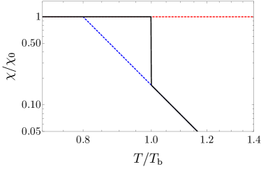
Fig. 1: Temperature dependence of $\chi(T)$ for $\Lambda/T_{{\mathrm{b}}}=0.8$ and $p=8$. The blue and red dashed lines represent $\chi$ in the false and true vacua, respectively.

For later convenience, we define the axion mass parameters by

$$m_{\phi}(T)\equiv\frac{\sqrt{\chi(T)}}{f_{\phi}}\ ,\quad m_{{\mathrm{b}}}\equiv\frac{\sqrt{\chi(T_{\mathrm{b}})}}{f_{\phi}}\ ,\quad m_{0}\equiv\frac{\sqrt{\chi_{0}}}{f_{\phi}}\ ,$$ (5)

and treat them as free parameters.

III Analysis of the spatially uniform case

The discontinuous change of the axion mass at the FOPT affects the axion abundance in the later universe. Here, we ignore the bubble dynamics and assume that the FOPT occurs uniformly in the universe. Then, we can divide the axion dynamics into three cases: $m_{\mathrm{b}}>3H_{\mathrm{b}}$, $m_{\mathrm{0}}>3H_{\mathrm{b}}>m_{\mathrm{b}}$, and $3H_{\mathrm{b}}>m_{0}$. Here, $H_{\mathrm{b}}\equiv H(T_{\mathrm{b}})$ is the Hubble parameter at $T=T_{\mathrm{b}}$. In the third case, the axion starts to oscillate after the FOPT, and the axion dynamics is the same as in the case where the axion has a constant mass $m_{0}$.

In the first case of $m_{\mathrm{b}}>3H_{\mathrm{b}}$, the axion starts to oscillate before the nucleation of bubbles. The temperature of the onset of oscillations, $T_{\mathrm{osc}}$, is estimated by

$$m_{\phi}(T_{\mathrm{osc}})=3H(T_{\mathrm{osc}})\ ,$$ (6)

which leads to

$$T_{\mathrm{osc}} \simeq\left(\sqrt{\frac{10}{\pi^{2}g_{*}(T_{\mathrm{osc}})}}m_{0}M_{\mathrm{Pl}}\Lambda^{p/2}\right)^{\frac{2}{p+4}}\ .$$ (7)

Here, we used the Friedmann equation during the radiation-dominated era,

$$3M_{\mathrm{Pl}}^{2}H^{2}=\frac{\pi^{2}}{30}g_{*}(T)T^{4}\ ,$$ (8)

with $M_{\mathrm{Pl}}\simeq 2.4\times 10^{18}$ GeV being the reduced Planck mass and $g_{*}$ being the relativistic degrees of freedom for the energy density. After then, the axion oscillates with a decreasing amplitude, $\bar{\phi}$. Until the phase transition, $\chi(T)$ evolves much slower than the oscillations of $\phi$. Then, the comoving number density of $\phi$ is conserved, and $\bar{\phi}$ is given by

$$\bar{\phi}\simeq\phi_{0}\sqrt{\frac{m_{\phi}(T_{\mathrm{osc}})}{m_{\phi}(T)}}\left(\frac{a_{\mathrm{osc}}}{a}\right)^{3/2}\ .$$ (9)

Ignoring the time evolution of the relativistic degree of freedom for the entropy density, $g_{*s}$, we obtain

$$\bar{\phi}(T)\simeq\phi_{0}\left(\frac{T}{T_{\mathrm{osc}}}\right)^{\frac{p+6}{4}}\ .$$ (10)

Consequently, $\phi$ can be approximated by

$$\phi\sim\phi_{0}\left(\frac{T}{T_{\mathrm{osc}}}\right)^{\frac{p+6}{4}}\sin\left[\int\mathrm{d}t\,m_{\phi}(T)\right]\ .$$ (11)

At the FOPT, we can approximate $\phi$ and $\dot{\phi}$ by

$$\phi \simeq\bar{\phi}_{\mathrm{b}}\sin\alpha_{\mathrm{b}}\ ,$$ (12)

$$\dot{\phi} \simeq m_{\mathrm{b}}\bar{\phi}_{\mathrm{b}}\cos\alpha_{\mathrm{b}}\ ,$$ (13)

where $\bar{\phi}_{\mathrm{b}}\equiv\bar{\phi}(T_{\mathrm{b}})$, and $\alpha_{\mathrm{b}}$ represents a phase of oscillations at the FOPT. Since the axion field oscillates with a mass of $m_{0}$ after the FOPT, the energy density of $\phi$ just after the FOPT is given by

$$\rho_{\phi}(T_{\mathrm{b}})=\frac{\bar{\phi}_{\mathrm{b}}^{2}}{2}\left(m_{\mathrm{b}}^{2}\cos^{2}\alpha_{\mathrm{b}}+m_{0}^{2}\sin^{2}\alpha_{\mathrm{b}}\right)\ .$$ (14)

Note that this assumes that both $\phi$ and $\dot{\phi}$ are preserved in FOPT. The condition for this will be clarified in the next section. One can see that, depending on $\alpha_{\mathrm{b}}$, $\rho_{\phi}$ can be enhanced at the phase transition. In particular, it is maximally enhanced by a factor of $m_{0}^{2}/m_{\mathrm{b}}^{2}$ when $\cos\alpha_{\mathrm{b}}=0$, but it remains unchanged at the phase transition if $\sin\alpha_{\mathrm{b}}=0$.

In the second case of $m_{\mathrm{0}}>{3H_{\mathrm{b}}}>m_{\mathrm{b}}$, the axion remains constant until the phase transition and begins to oscillate immediately afterward. Therefore, the energy density just after the phase transition is

$$\rho_{\phi}(T_{\mathrm{b}})=\frac{m_{0}^{2}\phi_{0}^{2}}{2}\ .$$ (15)

The sudden onset of oscillations has some similarities to the so-called trapped misalignment mechanism Higaki et al. (2016); Di Luzio et al. (2021); Jeong et al. (2022).

For comparison, we also consider the case of the second-order phase transition (or crossover) and evaluate the axion energy density for $T<\Lambda$. Here, we assume that the topological susceptibility follows Eq. (4). Then, the oscillation amplitude of the axion is given by Eq. (10) for $T>\Lambda$ and by

$$\bar{\phi}(T)\simeq\phi_{0}\left(\frac{\Lambda}{T_{\mathrm{osc}}}\right)^{\frac{p+6}{4}}\left(\frac{T}{\Lambda}\right)^{3/2}$$ (16)

for $T<\Lambda$, where we ignored the temperature dependence of $g_{*s}$. Thus, the axion energy density is given by

$$\rho_{\phi}^{\mathrm{2nd}}(T)\simeq\frac{m_{0}^{2}\phi_{0}^{2}}{2}\left(\frac{\Lambda}{T_{\mathrm{osc}}}\right)^{\frac{p+6}{2}}\left(\frac{T}{\Lambda}\right)^{3}\ .$$ (17)

We obtain the ratio of the axion energy density between the first- and second-order phase transitions as

$$\frac{\rho_{\phi}(T)}{\rho_{\phi}^{\mathrm{2nd}}(T)}=\frac{m_{\mathrm{b}}}{m_{0}}\cos^{2}\alpha_{\mathrm{b}}+\frac{m_{0}}{m_{\mathrm{b}}}\sin^{2}\alpha_{\mathrm{b}}\ ,$$ (18)

for $m_{\mathrm{b}}>3H(T_{\mathrm{b}})$ and

$$\frac{\rho_{\phi}(T)}{\rho_{\phi}^{\mathrm{2nd}}(T)}=\left(\frac{m_{\mathrm{b}}}{m_{0}}\right)^{\frac{6}{p}}\left(\frac{T_{\mathrm{osc}}}{\Lambda}\right)^{\frac{p+6}{2}}\ .$$ (19)

for $m_{\mathrm{0}}>3H(T_{\mathrm{b}})>m_{\mathrm{b}}$.

So far, for illustrative purposes, we have considered a setup in which the axion mass change due to FOPT is assumed to occur uniformly in space. In the next section, we will consider the effect of inhomogeneity due to bubble nucleation. On the other hand, sudden changes in axion mass that occur uniformly in space, as considered here, may occur in other situations. For example, if the axion mass is caused by the dynamics of another scalar field, a similar axion mass change could be realized by a certain choice of scalar potential.

IV Bubble-induced axion wave dynamics

IV.1 Classification of dynamics

So far, we have assumed that the FOPT takes place instantaneously and uniformly throughout the universe. In realistic situations, however, the bubble wall expands with a finite velocity, and we need to take into account spatial inhomogeneities of $\phi$. The time scale of the bubble expansion is given by $\beta^{-1}$, which is typically much shorter than the Hubble time at the bubble nucleation. In the following, we consider the axion dynamics in four cases:

1. $3H_{\mathrm{b}}>m_{0}$

2. $\beta>m_{0}>m_{\mathrm{b}},3H_{\mathrm{b}}$

3. $m_{\mathrm{b}}>\beta$

4. $m_{0}>\beta>m_{\mathrm{b}},3H_{\mathrm{b}}$

Here $\beta>H_{\mathrm{b}}$ and $m_{0}>m_{\mathrm{b}}$ are assumed. Cases (b) and (d) are further classified based on the relative magnitude of $m_{\mathrm{b}}$ and $3H_{\mathrm{b}}$.

In case (a), the axion starts to oscillate after the FOPT. Thus, the axion abundance can be evaluated in the same way as in the standard misalignment mechanism with a constant mass $m_{0}$. In case (b), the FOPT proceeds in a time scale shorter than the axion oscillation. Then, we can apply the evaluation in the previous section; we can use Eq. (18) for $m_{\mathrm{b}}>3H_{\mathrm{b}}$ and Eq. (19) for $m_{\mathrm{b}}<3H_{\mathrm{b}}$. In cases (c) and (d), the finite velocity of the bubble wall significantly affects the evolution of the axion field in different ways. In particular, the motion of bubble walls affects the axion field dynamics via two effects: the generation of axion waves and their reflection/transmission.

IV.2 Reflection and transmission

The effect of the passage of the bubble wall on the oscillating axion field can be analyzed in terms of the reflection and transmission of axion waves by the bubble wall. In practice, it will be necessary to analyze axion waves among randomly generated spherical bubble walls, but the essence of the dynamics can be understood in terms of reflection and transmission by planar bubble walls. In the following, we assume that the width of the wall in the wall rest frame is significantly smaller than the de Broglie wavelength of the axion, allowing us to model the wall as a step function in its direction of motion, specifically in the $z$-direction.

Let us discuss the reflection and transmission of axion waves at a single bubble wall. We show a schematic picture in Fig. 2. We consider a bubble wall moving along the $z$-axis and define the coordinate system $(t,z)$ such that the position of the wall is represented by $z=vt$. To analyze the transmission and reflection of waves, it is most convenient to move to the rest frame of the bubble wall $(t^{\prime},z^{\prime})$ given by

$$t^{\prime} =\gamma(t-vz)\ ,$$ (20)

$$z^{\prime} =\gamma(z-vt)\ ,$$ (21)

where $\gamma=1/\sqrt{1-v^{2}}$ is the Lorentz factor of the bubble wall. We consider an axion wave moving from the $z^{\prime}$-direction in the wall frame in the form

$$\Phi_{I}=\phi_{0}\exp[i(\omega^{\prime}t^{\prime}+k_{I}^{\prime}z^{\prime})]\ ,$$ (22)

where the real part of $\Phi$ corresponds to the axion field value. Then, a fraction of this axion wave, say $\Phi_{T}$, penetrates the wall, and the rest, $\Phi_{R}$, is reflected. On the wall, at $z^{\prime}=0$, we have the boundary conditions,

$$\Phi_{I}[t^{\prime},0]+\Phi_{R}[t^{\prime},0] =\Phi_{T}[t^{\prime},0]\ ,$$ (23)

$$\partial_{z^{\prime}}\Phi_{I}[t^{\prime},0]+\partial_{z^{\prime}}\Phi_{R}[t^{\prime},0] =\partial_{z^{\prime}}\Phi_{T}[t^{\prime},0]\ .$$ (24)

We then find the solution

$$\Phi_{R}[t^{\prime},z^{\prime}]=\frac{k_{I}^{\prime}-k_{T}^{\prime}}{k_{I}^{\prime}+k_{T}^{\prime}}\phi_{0}\exp[i(\omega^{\prime}t^{\prime}-k_{R}^{\prime}z^{\prime})]\ ,$$ (25)

$$\Phi_{T}[t^{\prime},z^{\prime}]=\frac{2k_{I}^{\prime}}{k_{I}^{\prime}+k_{T}^{\prime}}\phi_{0}\exp[i(\omega^{\prime}t^{\prime}+k_{T}^{\prime}z^{\prime})]\ ,$$ (26)

with

$$k_{R}^{\prime}=k_{I}^{\prime}\ ,\quad k_{T}^{\prime}=\sqrt{k_{I}^{\prime 2}+m_{\mathrm{b}}^{2}-m_{0}^{2}}\ .$$ (27)

This solution satisfies

$$k_{I}^{\prime}|\Phi_{I}[t^{\prime},0]|^{2}=k_{R}^{\prime}|\Phi_{R}[t^{\prime},0]|^{2}+k_{T}^{\prime}|\Phi_{T}[t^{\prime},0]|^{2}\ .$$ (28)

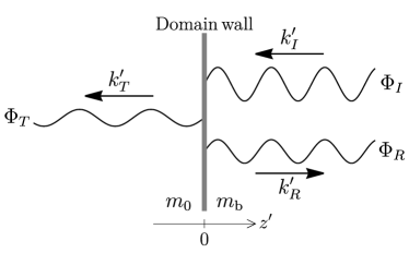
Fig. 2: Reflection and transmission of the axion wave in the wall frame.

In case (c), the axion field right before the bubble nucleation can be expressed as

$$\Phi_{I}(t,z)=\bar{\phi}_{\mathrm{b}}\exp[im_{\mathrm{b}}t]\ ,$$ (29)

in the cosmological frame. Here, we ignored the cosmic expansion because the FOPT typically proceeds in a time scale much shorter than the Hubble time. Then, moving to the wall frame, the axion becomes a wave moving from the $z^{\prime}$-direction in the form

$$\Phi_{I}(t^{\prime},z^{\prime})=\bar{\phi}_{\mathrm{b}}\exp[i(\omega_{0}^{\prime}t^{\prime}+k_{I0}^{\prime}z^{\prime})]\ ,$$ (30)

with

$$\omega_{0}^{\prime}=m_{\mathrm{b}}\gamma\ ,\quad k_{I0}^{\prime}=m_{\mathrm{b}}v\gamma\ .$$ (31)

Then, we obtain the momentum of the transmitted wave, $k_{T0}^{\prime}$, as

$${k_{T0}^{\prime}}=\sqrt{\gamma^{2}m_{\mathrm{b}}^{2}-m_{0}^{2}}\ .$$ (32)

When ${\rm Im}[k^{\prime}_{T0}]\neq 0$, the field damps inside the bubble, and the amplitudes of $\Phi_{R}$ and $\Phi_{I}$ are the same except for a phase shift, indicating total reflection of the axion wave. The reflected wave is then repeatedly scattered off another bubble wall, and when it gains enough energy, it is transmitted into the bubble. This acceleration by repeated reflections is similar to the Fermi acceleration Blandford and Ostriker (1978); Bell (1978); Drury (1983); Blandford and Eichler (1987), which will be studied next.

IV.3 Fermi acceleration

Let us continue with the $(1+1)$d spacetime simplification to describe the Fermi acceleration of the axion wave. We consider two walls moving towards each other at terminal velocity $v$. The wall moving in the $z$-direction is referred to as the “up wall”, and the other as the “down wall”. It is assumed that the axion wave continues to be completely reflected by the walls for a certain period.

Let us consider that a plain wave moves towards the up wall in the cosmological frame with a momentum $\{\omega,-k\}$. In the up wall frame, the axion wave has the four-momentum $\Lambda(-v)\cdot\{\omega,-k\}$ with

$$\Lambda(v)=\left(\begin{array}[]{cc}\gamma&v\gamma\\ v\gamma&\gamma\end{array}\right)\equiv\left(\begin{array}[]{cc}\cosh\psi&\sinh\psi\\ \sinh\psi&\cosh\psi\end{array}\right)\ ,$$ (37)

where $\psi$ is the rapidity defined by $\tanh\psi=v$. Then, this wave will be reflected, and the momentum becomes $\hat{P}\cdot\Lambda(-v)\cdot\{\omega,-k\}$, where $\hat{P}=\mathop{\rm diag}\nolimits{(1,-1)}$ denotes a parity transformation. In the cosmological frame, we get the momentum $\Lambda(v)\cdot\hat{P}\cdot\Lambda(-v)\cdot\{\omega,-k\}$. Then, this wave will be reflected by the down wall. With a similar transformation, we obtain the momentum in the cosmological frame after the second reflection as $\Lambda(-v)\cdot\hat{P}\cdot\Lambda(v)\cdot\Lambda(v)\cdot\hat{P}\cdot\Lambda(-v)\cdot\{\omega,-k\}$. By noting $\hat{P}\cdot\Lambda(v)\cdot\hat{P}=\Lambda(-v)$, we find the momentum in the cosmological frame after the $n$-th reflection

$$p_{\mu}[n] =\hat{P}^{n}\cdot\left(\Lambda(-v)\right)^{2n}\cdot\{\omega,-k\}$$

$$=\hat{P}^{n}\cdot\begin{pmatrix}\cosh(2n\psi)&\sinh(-2n\psi)\\ \sinh(-2n\psi)&\cosh(2n\psi)\end{pmatrix}\cdot\{\omega,-k\}.$$ (38)

Then, we get the angular frequency of the axion wave

$$p_{0}[n] =\frac{1}{2}\left[(\omega+k)\left(\frac{1+v}{1-v}\right)^{n}+(\omega-k)\left(\frac{1-v}{1+v}\right)^{n}\right]\ .$$ (39)

The enhancement of the angular frequency with $n\gg 1$ is given by the first term.

The next question concerns the number of possible reflections. For simplicity, we assume that the axion wave propagates at the speed of light. Let us consider an axion wave that undergoes its first reflection at the up wall when the walls are separated by a distance $L$ and denote the distance between the walls at the $n$-th reflection as $L_{\rm w}[n]$. The initial condition is $L_{\rm w}[1]=L$. Then it takes a time of $L/(v+1)$ for the axion waves to reach the down wall and undergo the second reflection. The $v$ in the denominator takes into account the motion of the down wall. During this interval, the distance between the walls decreases by $2vL/(v+1),$ and thus the distance at the second reflection is $L_{\rm w}[2]=L(1-2v/(1+v))=\frac{1-v}{1+v}L$. So at the $(n+1)$-th reflection we have $L_{\rm w}[n+1]=\left(\frac{1-v}{1+v}\right)^{n}L.$ This leads to

$$n=\frac{\log{\frac{L}{L_{\rm w}[n+1]}}}{\log{\frac{1+v}{1-v}}}.$$ (40)

By using this expression and taking $\omega=m_{\mathrm{b}}$ and $k=0$, we find

$$p_{0}[n]=\frac{m_{\mathrm{b}}}{2}\left(\frac{L}{L_{\rm w}[n+1]}+\frac{L_{\rm w}[n+1]}{L}\right).$$ (41)

This enhancement continues with large $n$ until the approximation becomes invalid, for instance when transmission becomes important as we will discuss soon, or the $L_{\rm w}$ becomes smaller than the wall width in the cosmological frame.

So far we have neglected transmission by assuming that $k_{T}^{\prime}$ is imaginary. However, reflection is not always perfect, especially when $n\gg 1$. For sufficiently large energies, $k_{T}^{\prime}$ becomes real, allowing transmission.

IV.4 Enhancement for axion abundance

In the spatially uniform case, the number density of the oscillating axion field increases by a factor of $m_{0}/m_{\rm b}$ in the FOPT Nakagawa et al. (2023). If we consider the effects of the bubble wall dynamics, the axion number is conserved in total reflection and not in transmission. The former is because in the wall rest frame the number (but not the density) is conserved at the reflection, and the total number in the symmetric phase is a Lorentz invariant, meaning it is conserved in the cosmic frame. The latter is because the bubble wall is so thin that the adiabatic condition is violated. Here we study the enhancement of the axion number during the FOPT, focusing on case (c).

As we have seen before, the transmission occurs when the angular frequency exceeds the mass inside the bubble:

$$\omega_{n}^{\prime}>m_{0},$$ (42)

where $\omega_{n}^{\prime}$ is the angular frequency after the $n$-th reflection with the wall in the wall frame. Similarly to the previous discussion, we can estimate $\omega_{n}^{\prime}$ as

$$\omega_{n}^{\prime} =a_{n}m_{\rm b}\ ,$$ (43)

$$a_{n} =\frac{1}{2}\left(\left(\sqrt{\frac{1+v}{1-v}}\right)^{2n-1}+\left(\sqrt{\frac{1-v}{1+v}}\right)^{2n-1}\right)\ .$$ (44)

Let us assume that the inequality (42) is first met when $n=n_{c}$. We show the dependence of $n_{c}$ on $v$ and $m_{0}/m_{\mathrm{b}}$ in Fig. 3.

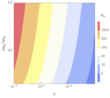
Fig. 3: Parameter dependence of $n_{c}$. The smaller $v$ and the larger $m_{0}/m_{\mathrm{b}}$, the larger $n_{c}$ becomes.

The amplitudes squared of the transmitted and reflected waves at the $(n_{c}+i)$-th collision are given by multiplying that of the incident waves at the $(n_{c}+i)$-th collision by a factor of $t_{i}$ and $r_{i}$ respectively, where $t_{i}$ and $r_{i}$ are given by

$$t_{i} =\left|\frac{2k_{I,n_{c}+i}^{\prime}}{k_{I,n_{c}+i}^{\prime}+k_{T,n_{c}+i}^{\prime}}\right|^{2},$$ (45)

$$r_{i} =\left|\frac{k_{I,n_{c}+i}^{\prime}-k_{T,n_{c}+i}^{\prime}}{k_{I,n_{c}+i}^{\prime}+k_{T,n_{c}+i}^{\prime}}\right|^{2}$$ (46)

with $k_{I,n}^{\prime}\equiv\sqrt{\omega_{n}^{\prime 2}-m_{\rm b}^{2}}$ and $k_{T,n}^{\prime}\equiv\sqrt{\omega_{n}^{\prime 2}-m_{0}^{2}}$. Thus, the sum of amplitude squared is enhanced through the Fermi acceleration process by a factor of

$$F=\sum_{i=0}F_{i},$$ (47)

where $F_{i}$ denotes the contribution from the axion wave that transmits the wall at the $(n_{c}+i)$-th collision and is given by

$$F_{0}\equiv t_{0}\ ,\quad F_{i}\equiv t_{i}r_{0}\cdots r_{i-1}\quad(i\geq 1).$$ (48)

For instance, for $v=0.1$, $m_{0}/m_{\rm b}=10$, we have $F\simeq 2.08$. See Fig. 4 for the contour of the enhancement factor due to the bubble wall dynamics.

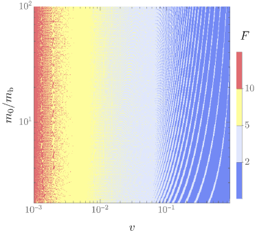
Fig. 4: Enhancement factor of the axion amplitude squared, $F$.

We also show $F_{i}$ in Fig. 5. For all the parameter sets there, $F_{i}$ decreases monotonically for $i$, and the maximum value $F_{0}$ is larger than unity. The decrease of $F_{i}$ is more significant for larger $v$, since a larger fraction of the axion wave can transmit the bubble wall for small $i$ due to the larger acceleration at each collision with the wall.

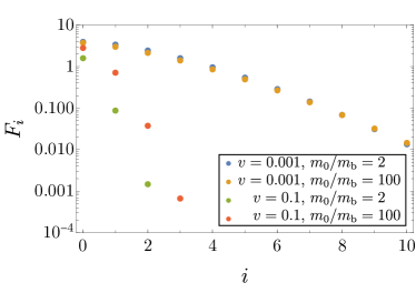
Fig. 5: Contribution to $F$ from the axion wave transmitted at the $(n_{c}+i)$-th collision, $F_{i}$.

To prepare for the evaluation of the axion abundance, we discuss the enhancement in the axion number. Since we are mainly interested in the axion abundance as non-relativistic matter in the later universe, we focus on the product of the axion mass and the amplitude squared as an effective axion number. While the axion mass changes from $m_{\mathrm{b}}$ to $m_{0}$ at the FOPT, the amplitude squared is enhanced by $F$. Thus, the axion number is effectively enhanced by $(m_{0}/m_{\mathrm{b}})F$, which we show in Fig. 6.

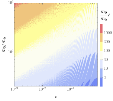
Fig. 6: Enhancement factor for the axion number density in the FOPT, $(m_{0}/m_{\mathrm{b}})F$.

The momentum distribution after the FOPT can also be estimated by boosting the transmitted momentum $k^{\prime}_{T,n}$ with $n\geq n_{c}$ in the wall frame to $k_{T,n}$ in the cosmological frame. The momentum distribution is proportional to the amplitude squared of the transmitted waves $\propto F_{i}$. Thus, the typical momentum of the transmitted waves can be estimated by $k_{T,n_{c}}$, which we show in Fig. 7. For $v<\mathcal{O}(0.1)$, $k_{T,n_{c}}$ is suppressed as $\sqrt{v}$. On the other hand, for $v>\mathcal{O}(0.1)$, $k_{T,n_{c}}$ can take a range of values including negative values, which mean the axion wave propagating outward in the bubble. This can be understood as follows. Since axion waves are significantly accelerated at each reflection, $k_{T,n_{c}}$ tends to be large. For some parameters, however, $\omega_{n_{c}}^{\prime}$ is slightly larger than $m_{0}$, and $k_{T,n_{c}}^{\prime}$ becomes much smaller than $m_{0}$. Then, moving to the cosmological frame, we obtain negative $k_{T,n_{c}}$.

Since the transmitted axion waves are typically non-relativistic or marginally non-relativistic, the spatial inhomogeneities of axion dark matter induced by FOPT could remain in the subsequent evolution of the universe.

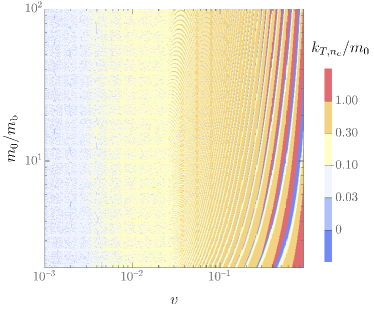
Fig. 7: Momentum of the transmitted wave for $n=n_{c}$, $k_{T,n_{c}}$.

The spatial scale of such fluctuations, $l$, can be estimated by the typical distance of the bubble walls when the $n_{c}$-th reflection occurs. In particular, for $v\ll 1$, we obtain

$$l\simeq R\left(\frac{1-v}{1+v}\right)^{n_{c}}\simeq\frac{v}{\beta}\frac{m_{\mathrm{b}}}{2m_{0}}\ ,$$ (49)

where we used

$$\omega_{n_{c}}^{\prime}\simeq\frac{1}{2}\left(\sqrt{\frac{1+v}{1-v}}\right)^{2n_{c}-1}m_{\mathrm{b}}\sim m_{0}\ .$$ (50)

The axion free-streams over a distance of $(k_{T,n_{c}}/m_{0})H_{\rm b}^{-1}$ during the Hubble time. If this is larger than $l$, the spatial inhomogeneities induced by the bubble wall dynamics are suppressed by the subsequent free streaming. Otherwise, the spatial inhomogeneities remain. This is the case if $\beta/H_{\rm b}$ is relatively small and the typical axion velocity is smaller than the wall velocity.

IV.5 Axion shock wave

In case (d), the axion does not oscillate outside the bubbles during the FOPT process. On the other hand, the axion mass inside the bubbles is large enough to affect the axion dynamics within the FOPT process.

First, we discuss analytically the axion dynamics just after bubble nucleation in case (d). We assume that the bubbles nucleate in a spherical shape and that the critical radius of the bubble is negligibly small compared to the cosmological scale. Then the axion field configuration becomes spherically symmetric and the equation of motion for the axion is given by

$$\left[\frac{\partial^{2}}{\partial t^{2}}+\frac{1}{r^{2}}\frac{\partial}{\partial r}\left(r^{2}\frac{\partial}{\partial r}\right)+m^{2}(t,r)\right]\phi(t,r)=0\ ,$$ (51)

which can be rewritten as

$$\left[\frac{\partial^{2}}{\partial t^{2}}+\frac{\partial^{2}}{\partial r^{2}}+m^{2}(t,r)\right]u(t,r)=0\ ,$$ (52)

Here $r$ is the radius, and we define $u\equiv r\phi$, and $m^{2}$ is the axion mass. In the following, we redefine the origin of the time coordinate so that $t=0$ corresponds to the bubble nucleation. Then, $m^{2}$ is given by

$$m^{2}(t,r)=\left\{\begin{array}[]{ll}m_{0}^{2}&\quad(0\leq r<vt)\\ m_{\mathrm{b}}^{2}&\quad(r>vt)\end{array}\right.\ .$$ (55)

Since $\beta>m_{\mathrm{b}}$, we can neglect $m_{\mathrm{b}}$ and approximate the initial condition as

$$\phi(t=0,r) =\phi_{\mathrm{b}}\ ,$$ (56)

$$\frac{\partial\phi}{\partial t}(t=0,r) =0\ .$$

In particular, if $m_{\mathrm{b}}<3H_{\mathrm{b}}$, we can use $\phi_{\mathrm{b}}=\phi_{0}$.

As the bubble expands, the axion inside the bubble evolves with a mass of $m_{0}$. If the bubble velocity is sufficiently smaller than the speed of light, the axion field near inside the bubble wall does not oscillate due to the gradient energy around the bubble wall. Then, the axion field inside the bubble settles to zero due to the mass. The depletion of the axion field value inside the bubble propagates with the speed of light to outside the bubbles with a decreasing amplitude. Consequently, we can approximate that the axion field changes its value from $0$ at $r=vt$ to $\phi_{\mathrm{b}}$ at $r=t$. By using these boundary conditions, we can solve the axion field configuration in $vt<r<t$ and obtain an approximate solution as 

$$\phi(t,r)\simeq\left\{\begin{array}[]{ll}0&\quad(0\leq r<vt)\\ \left[1-\frac{v(t-r)}{(1-v)r}\right]\phi_{\mathrm{b}}&\quad(vt\leq r<t)\\ \phi_{\mathrm{b}}&\quad(r\geq t)\end{array}\right.\ .$$ (60)

We show in Fig. 8 the numerical result and the approximate solution, and it can be seen that they are in good agreement with each other.

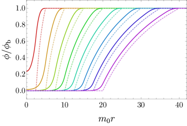
Fig. 8: Evolution of the axion field in case (d) with $v=0.5$. The solid and dashed lines represent the numerical result and the approximate solution, respectively. The results are shown for $5\leq m_{0}t\leq 40$ at intervals of $m_{0}\Delta t=5$.

We estimate the axion number density after the FOPT. The energy of the radiated axion wave is given by

$$E_{\phi} \equiv 4\pi\int_{vt}^{r}\mathrm{d}r\,r^{2}\frac{(\partial_{t}\phi)^{2}+(\partial_{r}\phi)^{2}}{2}$$

$$\simeq 2\pi\frac{v(1+v)}{1-v}\phi_{\mathrm{b}}^{2}t\ .$$ (61)

The typical momentum of the axion field is given by

$$k_{\mathrm{typ}} \equiv\left.\frac{\partial_{r}\phi}{\phi}\right|_{r=(1+v)t/2}\simeq\frac{4v}{(1-v^{2})t}\ .$$ (62)

Then, the axion number associated with a single bubble before collisions is estimated by

$$N_{\phi}\equiv\frac{E_{\phi}}{k_{\mathrm{typ}}}\simeq\frac{\pi\phi_{\mathrm{b}}^{2}}{2}(1+v)^{2}t^{2}\ .$$ (63)

Assuming that the axion number is approximately conserved in reflections and transmissions with the bubble wall, we obtain the axion number density after the FOPT as

$$n_{\phi}\equiv\frac{N_{\phi}}{L^{3}}\simeq\frac{\pi\phi_{\mathrm{b}}^{2}}{2L}\ ,$$ (64)

where we assumed $t=L/(1+v)$ as a typical time when the axion wave first scatters off the bubble wall and neglected the velocity dependence because it depends strongly on how the typical momentum is chosen. It is very important to note that the density of axion numbers is inversely proportional to the distance $L$ between bubbles. This indicates that as the distance between bubbles increases, the production of axion numbers decreases. This phenomenon occurs because in case (d) the axion waves are restricted to the region just outside the bubbles, in contrast to case (c), where the axion waves are spread over the entire space.

We will confirm these observations in numerical simulations.

IV.6 Numerical results

Due to the complexity of the dynamics of axion waves, numerical lattice calculation is essential to study them in a more realistic setting than those modeled by planar walls or spherical axion waves. Here, for simplicity, we focus on case (d) with $m_{\rm b}=0$, neglecting the cosmic expansion, and perform numerical lattice calculations to confirm that the analytical estimate well describes the axion abundance in the final stage of the transition.

In the three-dimensional lattice simulations, we have set a bubble nucleated at the center of the lattice box and imposed the periodic boundary condition. This implies that bubble nucleation points are aligned with the equal separations determined by the lattice box size $L_{\rm box}$, which corresponds to $v/\beta$. Here the expansion of the universe and the mass outside the bubble are neglected, assuming $\beta\gg m_{\rm b},3H_{\rm b}$.

The equation of motion is given by

$$\left[\frac{\partial^{2}}{\partial t^{2}}+\bm{\nabla}^{2}+m^{2}(t,\bm{x})\right]\phi(t,\bm{x})=0.$$ (65)

Here, the mass squared of the axion is set to be

$$m^{2}(t,\bm{x})=\frac{1-\tanh{((r-vt)/\delta_{w})}}{2}\times m_{0}^{2},$$ (66)

where $r$ is the distance from the bubble nucleation point and $\delta_{w}$ determines the thickness of the bubble wall in the rest frame of the bubble nucleation point, not in the wall rest frame. In all simulations, we choose $\delta_{w}=0.15m_{0}^{-1}$, which is smaller than the typical de Broglie wavelength of the axion wave. We have checked that thinning the wall does not significantly change the results.

The parameter settings for the simulations are summarized in Table. 1. Each simulation starts with the homogeneous initial condition $\phi=\phi_{0}$ and ends at $t_{\rm end}=L_{\rm box}/v$, sufficiently later than the end of the phase transition.

We show an example of the time evolution of the axion’s energy density in Fig. 9. The solid line is the total energy density of the axion, while the dotted line is the contribution of the bubbles, the energy inside the bubbles divided by the total volume. Each bounce corresponds to the reflection and transmission of the axion waves, so the interval decreases as the bubble wall approaches the nearest wall. The Fermi acceleration appears as an increase in the energy density outside the bubble, and as the energy increases, the transmission into the bubble becomes more prominent.

Through simulations, we have calculated the axion number density after the end of the phase transition, $n_{\phi}$, which is given by

$$n_{\phi}=\frac{1}{V}\int\frac{{\rm d}^{3}\bm{k}}{(2\pi)^{3}2\omega_{k}}\left[\dot{\tilde{\phi}}^{2}+\omega_{k}^{2}\tilde{\phi}^{2}\right],$$ (67)

where $\tilde{\phi}(t,\bm{k})$ is the Fourier transform of $\phi(t,\bm{x})$, $V=L_{\rm box}^{3}$ is the volume of the system, and $\omega_{k}\equiv\sqrt{\bm{k}^{2}+{m_{0}^{2}}}$. We show in Fig. 10 the numerical results of the axion’s number density $n_{\phi}$ for the box size $L_{\rm box}$. The circular, square, and triangular points correspond to the results of $v=0.1\,,0.5$, and $0.9$ respectively. The black dotted line is proportional to $L_{\rm box}^{-1}$. We can observe the excellent agreement with the power law expected in Eq. (64).

Case	$(m_{0}L_{\rm box})^{3}$	${N_{\rm grid}}^{3}$	$v$	$m_{0}t_{\rm end}$
(v1-1)	$(2\pi)^{3}$	$128^{3}$	0.1	62.8
(v1-2)	$(4\pi)^{3}$	$256^{3}$	0.1	126.7
(v1-3)	$(8\pi)^{3}$	$512^{3}$	0.1	251.3
(v1-4)	$(16\pi)^{3}$	$1024^{3}$	0.1	502.7
(v5-1)	$(2\pi)^{3}$	$128^{3}$	0.5	12.6
(v5-2)	$(4\pi)^{3}$	$256^{3}$	0.5	25.1
(v5-3)	$(8\pi)^{3}$	$512^{3}$	0.5	50.3
(v5-4)	$(16\pi)^{3}$	$1024^{3}$	0.5	100.5
(v9-1)	$(2\pi)^{3}$	$128^{3}$	0.9	7.0
(v9-2)	$(4\pi)^{3}$	$256^{3}$	0.9	14.0
(v9-3)	$(8\pi)^{3}$	$512^{3}$	0.9	27.9
(v9-4)	$(16\pi)^{3}$	$1024^{3}$	0.9	55.9

Table. 1: The parameter setup for the 3D lattice simulations.

Fig. 9: The time evolution of the energy of the system in the case (v1-3) where $L_{\rm box}=8\pi m_{0}^{-1}$ and $v=0.1$. The solid line represents the total average energy density, whereas the dotted line is the energy density inside the bubble times the volume fraction of the bubble.

Fig. 10: The axion number density at the final time as a function of the box size for $v=0.1,0.5$ and $0.9$. The dotted line is the line proportional to $L_{\rm box}^{-1}$.

Since the wall velocity dependence of the final number density does not vary significantly for different $L_{\rm box}$ in Fig. 10, we have studied the axion number density for different wall velocities, fixing $L_{\rm box}=16\pi m_{0}^{-1}$ and $N_{\rm grid}=1024$. The results are shown in Fig. 11. The number density behaves differently in the high-velocity region and the low-velocity region pivoting $v\sim 0.4$. Two dashed lines represent the result of piecewise power law fits. The fitted results are given by

$$n_{\phi}=Cv^{\alpha}\frac{\phi_{0}^{2}}{L_{\rm box}},$$ (68)

with

$$C\simeq\left\{\begin{array}[]{ll}1.3&\quad(v\lesssim 0.4)\\ 1.8&\quad(v\gtrsim 0.4)\end{array}\right.,\quad\alpha\simeq\left\{\begin{array}[]{ll}0.4&\quad(v\lesssim 0.4)\\ 0.8&\quad(v\gtrsim 0.4)\end{array}\right..$$ (69)

Thus, these numerical results agree well with the analytical estimate in Eq. (64).

We show in Fig. 12 the momentum distribution of the created axion number, $n(k)$, at the final time of each simulation where the box size is fixed, $L_{\rm box}=16\pi m_{0}^{-1}$. Here $n(k)$ is defined by

$$n(k)=\frac{k^{3}}{2\pi^{2}\cdot 2\omega_{k}V}\left[\dot{\tilde{\phi}}^{2}+\omega_{k}^{2}\tilde{\phi}^{2}\right],$$ (70)

where $k\equiv|{\bm{k}}|$ assuming the rotational symmetry, so that $n_{\phi}=\int{\rm d}\ln{k}\,n(k)$. We can see that the generated axions are marginally non-relativistic, and that the peak momentum of the axion increases with the wall velocity, which makes sense since the axion gains more energy with each reflection.

Fig. 11: The axion number density at the final time for the bubble velocity.

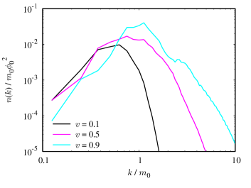
Fig. 12: The momentum distribution of the axion number density after the end of the phase transition. Three lines correspond to the result with the wall velocity $v=0.1$ (black), $0.5$ (magenta), and $0.9$ (cyan), and we set $L_{\rm box}=16\pi m_{0}^{-1}$.

V Bubble misalignment mechanism

V.1 Scenario overview

Before calculating the axion abundance, let us first discuss the axion dynamics in the four cases we have classified, based on the results of the previous section. For readability, the four cases are noted here again: (a) $3H_{\mathrm{b}}>m_{0}$; (b) $\beta>m_{0}>m_{\mathrm{b}},3H_{\mathrm{b}}$; (c) $m_{\mathrm{b}}>\beta$; (d) $m_{0}>\beta>m_{\mathrm{b}},3H_{\mathrm{b}}$.

In case (a), the axion does not oscillate even after the FOPT is completed but starts to oscillate after a while. The misalignment mechanism works as in the case where the axion mass has a constant value of $m_{0}$.

On the other hand, in case (b) the axion does not move during the FOPT, but starts oscillating with the mass $m_{0}$ immediately afterwards. For $m_{\mathrm{b}}<3H(T_{\mathrm{b}})$, the axion did not start oscillating before the FOPT. Let us call this case (b1). This situation corresponds to that studied in Ref. Nakagawa et al. (2023) and is similar to the trapped misalignment mechanism Higaki et al. (2016); Di Luzio et al. (2021); Jeong et al. (2022). For $m_{\mathrm{b}}>3H(T_{\mathrm{b}})$, the axion has already started oscillating before the FOPT. Let us call this case (b2). In cases (a) and (b), bubbles do not significantly affect the axion dynamics.

The bubble plays an interesting and crucial role in cases (c) and (d). In case (c), the axion has already started oscillating before the FOPT, and the nucleated bubbles expel axions from the inside if $m_{0}>\gamma m_{\mathrm{b}}$ (see Eq. (32)). These axion waves outside the bubbles repeatedly scatter off the bubble walls until they acquire enough energy to enter the bubbles. In this Fermi acceleration process, the axion number is conserved, except for the last entry into the bubbles, where the axion number can be increased depending on the bubble wall velocity. As can be seen in Fig. 4, the enhancement is at most several times for the bubble wall velocity of ${\cal O}(0.1)$.

In case (d), the axion has not yet started oscillating before the FOPT. It is further classified into cases (d1) and (d2) for $m_{\mathrm{b}}<3H(T_{\mathrm{b}})$ and $m_{\mathrm{b}}>3H(T_{\mathrm{b}})$, respectively. In case (d), as the bubbles nucleate, the axions are expelled from the inside of the bubbles, similar to case (c). The difference is that outside the bubbles, the axion forms a kind of shock wave, and their momentum decreases as they propagate. Accordingly, the effective number of axions changes over time until they finally enter the bubbles after acquiring enough energy through Fermi acceleration. In contrast to case (c), the resultant axion abundance is a decreasing function of the typical size of the bubbles because the axion shock wave exists only near the surface of the bubbles. However, in case (c), the axion is already oscillating throughout space before the FOPT.

V.2 Axion abundance

Here, we summarize the predictions for axion abundance in each case. For simplicity, we assume that the universe is radiation-dominated, where all components in the plasma have the same temperature. It is straightforward to estimate axion abundance during a matter-dominated era, such as the inflaton oscillation period, or in cases where the hidden gauge sector has a different temperature from the standard model plasma.

First, we evaluate the axion abundance in the second-order phase transition. Assuming the topological susceptibility given in Eq. (4), we obtain

$$\frac{\rho_{\phi}^{\mathrm{(2nd)}}}{s} =\frac{\frac{1}{2}m_{0}m_{\phi}(T_{\mathrm{osc}})\phi_{0}^{2}}{\frac{2\pi^{2}g_{*s,\mathrm{osc}}}{45}T_{\mathrm{osc}}^{3}}$$

$$=\frac{45}{4\pi^{2}g_{*s,\mathrm{osc}}}\left(\frac{\pi^{2}g_{*,\mathrm{osc}}}{10}\right)^{\frac{p+6}{2(p+4)}}\frac{m_{0}^{\frac{p+2}{p+4}}\phi_{0}^{2}}{M_{\mathrm{Pl}}^{\frac{p+6}{p+4}}\Lambda^{\frac{p}{p+4}}}$$

$$=\frac{45}{4\pi^{2}g_{*s,\mathrm{osc}}}\left(\frac{\pi^{2}g_{*,\mathrm{osc}}}{10}\right)^{\frac{p+6}{2(p+4)}}\frac{m_{0}\phi_{0}^{2}}{(m_{\mathrm{b}}^{2}M_{\mathrm{Pl}}^{p+6}T_{\mathrm{b}}^{p})^{\frac{1}{p+4}}}\ .$$ (71)

Here and in the following, $g_{*s,\mathrm{osc}}$ represents the effective number of relativistic species contributing to the entropy, evaluated at the moment when the axion first begins to oscillate.

In case (a), the axion does not start oscillating yet at FOPT, but starts oscillating at $m_{0}\sim 3H$. The temperature at the onset of oscillations is given by

$$T_{\mathrm{osc,(a)}}\simeq\left(\frac{10}{\pi^{2}g_{*,\mathrm{osc}}}\right)^{1/4}\sqrt{M_{\mathrm{Pl}}m_{0}}\ .$$ (72)

Then, we obtain

$$\frac{\rho_{\phi}^{\mathrm{(a)}}}{s} =\frac{\frac{1}{2}m_{0}^{2}\phi_{0}^{2}}{\frac{2\pi^{2}g_{*s,\mathrm{osc}}}{45}T_{\mathrm{osc,(a)}}^{3}}$$

$$=\frac{45}{4\pi^{2}g_{*s,\mathrm{osc}}}\left(\frac{\pi^{2}g_{*,\mathrm{osc}}}{10}\right)^{3/4}\frac{m_{0}^{1/2}\phi_{0}^{2}}{M_{\mathrm{Pl}}^{3/2}}\ .$$ (73)

This is of course equal to the axion abundance when the mass of the axion is constant at $m_{0}$.

In case (b), from the discussion in Sec. III, we obtain

$$\frac{\rho_{\phi}^{\mathrm{(b1)}}}{s} =\frac{\frac{m_{0}^{2}\phi_{0}^{2}}{2}}{\frac{2\pi^{2}g_{*s,\mathrm{osc}}}{45}T_{\mathrm{b}}^{3}}$$

$$=\frac{45m_{0}^{2}\phi_{0}^{2}}{4\pi^{2}g_{*s,\mathrm{osc}}T_{\mathrm{b}}^{3}}\ ,$$ (74)

for $m_{\mathrm{b}}<3H(T_{\mathrm{b}})$ and

$$\frac{\rho_{\phi}^{\mathrm{(b2)}}}{s} =\frac{\frac{\phi_{0}^{2}}{2}\frac{m_{\phi}(T_{\mathrm{osc,(b2)}})}{m_{\mathrm{b}}}}{\frac{2\pi^{2}g_{*s,\mathrm{osc}}}{45}T_{\mathrm{osc,(b2)}}^{3}}\left(m_{\mathrm{b}}^{2}\cos^{2}\alpha_{\mathrm{b}}+m_{0}^{2}\sin^{2}\alpha_{\mathrm{b}}\right)$$

$$=\frac{45}{4\pi^{2}g_{*s,\mathrm{osc}}}\left(\frac{\pi^{2}g_{*,\mathrm{osc}}}{10}\right)^{\frac{p+6}{2(p+4)}}\frac{\phi_{0}^{2}}{(m_{\mathrm{b}}^{p+6}M_{\mathrm{Pl}}^{p+6}T_{\mathrm{b}}^{p})^{\frac{1}{p+4}}}$$

$$\phantom{=}\times\left(m_{\mathrm{b}}^{2}\cos^{2}\alpha_{\mathrm{b}}+m_{0}^{2}\sin^{2}\alpha_{\mathrm{b}}\right)\ ,$$ (75)

for $m_{\mathrm{b}}>3H(T_{\mathrm{b}})$.

In case (c), the axion number is enhanced by $(m_{0}/m_{\mathrm{b}})F$ due to the Fermi acceleration. Thus, we obtain

$$\frac{\rho_{\phi}^{\mathrm{(c)}}}{s} =\frac{\frac{1}{2}m_{0}m_{\phi}(T_{\mathrm{osc,(c)}})\phi_{0}^{2}}{\frac{2\pi^{2}g_{*s,\mathrm{osc}}}{45}T_{\mathrm{osc,(c)}}^{3}}\frac{m_{0}}{m_{\mathrm{b}}}F$$

$$=\frac{45}{4\pi^{2}g_{*s,\mathrm{osc}}}\left(\frac{\pi^{2}g_{*,\mathrm{osc}}}{10}\right)^{\frac{p+6}{2(p+4)}}\frac{Fm_{0}^{2}\phi_{0}^{2}}{(m_{\mathrm{b}}^{p+6}M_{\mathrm{Pl}}^{p+6}T_{\mathrm{b}}^{p})^{\frac{1}{p+4}}}\ .$$ (76)

Case (d) can be further classified into case (d1) for $m_{\mathrm{b}}<3H(T_{\mathrm{b}})$ and case (d2) for $m_{\mathrm{b}}>3H(T_{\mathrm{b}})$. We estimate the axion abundance in case (d1) using the numerical results. In the numerical simulations, the adjacent bubble is separated by a distance of $L_{\mathrm{box}}$. Thus, we estimate the axion number density just after the FOPT as

$$n_{\phi}(T_{\mathrm{b}})\simeq Cv^{-1+\alpha}\beta\phi_{0}^{2}$$ (77)

by setting $L_{\mathrm{box}}=v/\beta$. Then, we obtain the axion energy density in the later universe as

$$\frac{\rho_{\phi}^{\mathrm{(d1)}}}{s} \simeq\frac{Cv^{-1+\alpha}\beta m_{0}\phi_{0}^{2}}{\frac{2\pi^{2}g_{*s,\mathrm{b}}}{45}T_{\mathrm{b}}^{3}}$$

$$=\frac{45Cv^{-1+\alpha}\beta m_{0}\phi_{0}^{2}}{2\pi^{2}g_{*s,\mathrm{b}}T_{\mathrm{b}}^{3}}\ ,$$ (78)

where $g_{*s,\mathrm{b}}\equiv g_{*s}(T_{\mathrm{b}})$.

On the other hand, in case (d2), the axion field at the FOPT has a degree of freedom of $\alpha_{\mathrm{b}}$ as in case (b2). If $\dot{\phi}=0$ at the FOPT, the axion dynamics during the FOPT process will be the same as in case (d1), and the axion abundance is given by

$$\frac{\rho_{\phi}^{\mathrm{(d2\text{-}1)}}}{s} \simeq\frac{Cv^{-1+\alpha}\beta m_{0}\bar{\phi}_{\mathrm{b}}^{2}}{\frac{2\pi^{2}g_{*s,\mathrm{b}}}{45}T_{\mathrm{b}}^{3}}$$

$$=\frac{45Cv^{-1+\alpha}\beta m_{0}\phi_{0}^{2}}{2\pi^{2}g_{*s,\mathrm{b}}T_{\mathrm{b}}^{3}}\left(\frac{T_{\mathrm{b}}}{T_{\mathrm{osc}}}\right)^{(p+6)/2}$$

$$=\frac{45Cv^{-1+\alpha}}{2\pi^{2}g_{*s,\mathrm{b}}T_{\mathrm{b}}^{3}}\left(\frac{\pi^{2}g_{*,\mathrm{osc}}}{10}\right)^{\frac{p+6}{2(p+4)}}\frac{\beta m_{0}\phi_{0}^{2}T_{\mathrm{b}}^{\frac{p+6}{2}}}{(m_{0}M_{\mathrm{Pl}}\Lambda^{\frac{p}{2}})^{\frac{p+6}{p+4}}}$$

$$=\frac{45Cv^{-1+\alpha}}{2\pi^{2}g_{*s,\mathrm{b}}}\left(\frac{\pi^{2}g_{*,\mathrm{osc}}}{10}\right)^{\frac{p+6}{2(p+4)}}\frac{\beta m_{0}\phi_{0}^{2}}{(m_{\mathrm{b}}^{p+6}M_{\mathrm{Pl}}^{p+6}T_{\mathrm{b}}^{p})^{\frac{1}{p+4}}}\ .$$ (79)

If $\phi=0$ at the FOPT, the passage of the bubble wall does not change $\phi$ and $\dot{\phi}$. In this case, the axion abundance becomes the same as in case (b2).

$$\frac{\rho_{\phi}^{\mathrm{(d2\text{-}2)}}}{s} =\left.\frac{\rho_{\phi}^{\mathrm{(b2)}}}{s}\right|_{\sin\alpha_{\mathrm{b}}=0}\ .$$ (80)

Depending on the phase of the oscillation at the FOPT, the axion abundance will be between Eqs (79) and (80).

We show the dependence of $\rho_{\phi}/s$ on $m_{0}$ in Fig. 13. Here, we fixed $\beta/H_{\mathrm{b}}$ and $m_{0}/m_{\mathrm{b}}$ satisfying $\beta/(3H_{\mathrm{b}})>m_{0}/m_{\mathrm{b}}$. Then, case (b2) is realized, and if $\beta/(3H_{\mathrm{b}})<m_{0}/m_{\mathrm{b}}$, case (d1) is realized instead of case (b2).

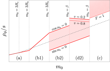
Fig. 13: Axion abundance $\rho_{\phi}/s$. The red and gray-dashed lines represent the results for the first- and second-order phase transition, respectively.

Let us also estimate the axion-photon coupling $g_{\phi\gamma\gamma}$ to explain all dark matter. If $\rho_{\phi}/s\simeq 0.44$ eV, the axion accounts for all dark matter. Once we fix all the parameters other than $\phi_{0}$, we obtain $\phi_{0}$ for all dark matter. Here, we assume $\phi_{0}=f_{\phi}$ and $g_{\phi\gamma\gamma}=\alpha/(2\pi f_{\phi})$. Then, we can obtain $g_{\phi\gamma\gamma}$ for axion dark matter by fixing the parameters of the axion mass and FOPT. In particular, we consider the upper bound on $g_{\phi\gamma\gamma}$. From the Lyman-$\alpha$ data, the redshift of the dark matter formation is constrained as $z\gtrsim z_{\mathrm{min}}\sim 10^{6}$ Sarkar et al. (2015). Here, we require that the axion starts to oscillate and the axion mass becomes constant before $z=z_{\mathrm{min}}$. Then, we obtain the minimum value of $f_{\phi}$ for axion dark matter, which leads to the maximum value of $g_{\phi\gamma\gamma}$. We show the maximum $g_{\phi\gamma\gamma}$ for axion dark matter in Fig. 14. Here, we used $g_{*}$ and $g_{*s}$ given in Ref. Husdal (2016). In case (a), the axion abundance is determined only by $m_{0}$ and $\phi_{0}$, and thus the line for case (a) (red) does not depend on $z_{\mathrm{min}}$. In cases (b1), (b2), (c), (d1), and (d2-1), we obtained the upper bound by assuming $T_{\mathrm{b}}=T_{\mathrm{min}}$, where $T_{\mathrm{min}}\simeq 2.3\times 10^{2}$ eV is the cosmic temperature when $z=z_{\mathrm{min}}$. For comparison, we also show the result for the second-order phase transition, where we assumed $\Lambda=T_{\mathrm{min}}$.

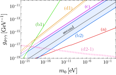
Fig. 14: Upper bound on $g_{\phi\gamma\gamma}=\alpha/(2\pi f_{\phi})$ for axion dark matter in each scenario. We set $\phi_{0}=f_{\phi}$ and $p=8$. The red, green, blue, purple, orange, and pink lines represent cases (a), (b1), (b2), (c), (d1), and (d2-1), respectively. For cases (b1), (b2), (c), (d1), and (d2-1), we use $T_{\mathrm{b}}=T_{\mathrm{min}}\simeq 2.3\times 10^{2}$ eV to derive the upper bound. We also set $m_{0}/m_{\mathrm{b}}=100$ for cases (b2), (c), and (d2-1), and $\beta/(3H_{\mathrm{b}})=10^{3}$ for cases (d1) and (d2-1). Cases (d1) and (d2-1) are shown in the solid and dotted lines for $v=0.2$ and $v=0.8$, respectively. The blue-shaded region reflects the $\alpha_{\mathrm{b}}$-dependence of $\rho_{\phi}$ in case (b2). The purple-shaded region corresponds to $1\leq F\leq 5$ in case (c). Note that case (c) with $F=1$ coincides with the upper line for case (b2). For comparison, we also show the result for the second-order phase transition assuming $\Lambda=T_{\mathrm{min}}$ with the gray line. Cases (b2), (c), and (d2) cannot be realized on the dashed lines for $T_{\mathrm{b}}=T_{\mathrm{min}}$, $m_{0}/m_{\mathrm{b}}=100$, and $\beta/(3H_{\mathrm{b}})=10^{3}$.

VI Summary and discussions

In this paper, we have studied the axion dynamics during the FOPT in which the axion mass changes discontinuously. In particular, we have taken into account the bubble wall dynamics for the first time and found that the axions can be expelled from the inside of the expanding bubbles when the axion mass inside the bubble is larger than $\beta$. This leads to a phenomenon analogous to Fermi acceleration, where the axion waves are repeatedly accelerated in collisions with the bubble walls until they gain sufficient energy to penetrate the wall. Furthermore, we have found that the axion abundance is further increased by an order of magnitude when the axions enter the bubbles after repeated acceleration.

We have estimated the axion abundance, which turns out to be significantly larger than in the case where the axion mass is constant.

The momentum distribution of the axions after the FOPT is marginally relativistic for the relativistic bubble wall velocity and becomes nonrelativistic for low velocity. Thus the spatial inhomogeneities of axions generated during the FOPT are likely to be erased by the free streaming afterwards. Depending on the detailed process during the FOPT, however, it might be possible to have relatively large inhomogeneities. For instance, if $\beta$ is of order unity and the bubble wall velocity is low, the resultant axions are marginally nonrelativistic, and we expect that large inhomogeneities will persist on relatively large scales within the Hubble horizon, leading to the formation of the axion minicluster.

Another immediate consequence of the nonzero modes excited during FOPT could be to hinder the formation of oscillons/I-balls Bogolyubsky and Makhankov (1976); Segur and Kruskal (1987); Gleiser (1994); Copeland et al. (1995); Gleiser and Sornborger (2000); Honda and Choptuik (2002); Kasuya et al. (2003), which are expected to occur efficiently if the onset of spatially homogeneous oscillations is delayed Jeong et al. (2022); Nakagawa et al. (2023). This is because the formation of these non-topological solitons requires coherence over a region much larger than the inverse of the axion mass. On the other hand, the production of vector bosons coupled to axions may still proceed even in the presence of spatial inhomogeneities. Then, one may be able to produce the right amount of dark photon dark matter without introducing a large coupling, similar to Ref. Kitajima and Takahashi (2023) (see also Refs. Agrawal et al. (2020); Co et al. (2019); Bastero-Gil et al. (2019)). One can also apply the axion dynamics during FOPTs to explain the recent hint of isotropic cosmic birefringence Minami and Komatsu (2020); Diego-Palazuelos et al. (2022); Eskilt (2022); Eskilt and Komatsu (2022). For example, if the solar system is in a bubble formed after recombination and the axion waves have not yet transmitted much into the bubble, we will observe isotropic cosmic birefringence. It will be interesting to explore the viable parameter range.

While we have focused on the axion abundance, the dark glueballs could also contribute to dark matter. As discussed in Ref. Nakagawa et al. (2023), the dark glueball abundance might be reduced by the coupling to the axion. One can also introduce dark quarks with dark photon couplings so that the dark pion can decay or annihilate into the dark photons to cool the dark sector.

So far we have considered the dynamics of the axion, whose mass changes significantly during the FOPT, but the same argument can be straightforwardly applied to any scalar field whose mass changes during the FOPT or similar transitions induced by other fields. Thus, phenomena such as the Fermi acceleration found in this paper may be quite general in the scalar dynamics during phase transitions, and it could have interesting applications such as the production of warm dark matter, boson star formation, cosmic birefringence, baryogenesis, etc.

Let us comment on an implicit assumption made in this paper relevant to large $N$ Yang-Mills theory and the possible extension beyond the assumption. In Yang-Mills theory coupled to the axion, the potential of the axion can be either single-valued or multi-valued Witten (1980). So far we have implicitly assumed the former possibility. In particular, if we consider ${\rm SU{(}}N)$ Yang-Mills theory with large $N$, we may have the latter case, because in chiral perturbation theory, one expects a $(\log[\det U])^{2}$ term, which is multi-valued, for the $\eta^{\prime}$ mass in the large $N$ limit, where $U$ is the matrix relevant for the Nambu-Goldstone boson. Let us comment on the cosmology with the latter possibility, which will turn out to be interesting. By integrating out the mesons, the axion potential is of the form $V_{i}(a/(Nf_{a}))=V_{0}(a/(Nf_{a})+i/N)$, where $i$ is the label relevant for different branches, with the combination $a/(Nf_{a})$ appearing in the large $N$ limit. $V_{0}$ represents the potential form for each branch. Thanks to the multi-valued potential, the symmetry $a\to a+2\pi f_{a}$ is preserved, although it is violated for each potential.

Recovering the heavy meson potential, we find in the full potential that different branches are separated by potential barriers. Since $V_{i}$ has the same shape and minimum value for different $i$, this implies that the setup contains axion domain wall configurations. Thus, in cosmology, the domain walls may be produced and collapse due to the potential or population bias. This contribution could affect the final abundance of axion dark matter, which will be an interesting topic for future studies in this direction.

So far, we have had analytical discussions on the case that the wall width in the wall rest frame is much smaller than the axion wavelength. In the opposite limit, which, although is a slightly unnatural setup for a light axion dark matter, analytical estimations are also possible following Refs. Azatov and Vanvlasselaer (2021); Azatov et al. (2021b). Since the wavelength is much shorter than the wall width, the shape of the wall is important for discussing the transmission rate or reflection rate. In this case, we can use the WKB approximation. Axion could be considered as a particle. Still, the energy conservation is valid across the wall at the wall rest frame. The transmission/reflection probability can be estimated by quantum mechanics. For simplicity, when the momentum is larger than the axion mass scales, the amplitude can be approximated as ${\cal M}\sim\int\mathrm{d}z^{\prime}\frac{1}{2w^{\prime}}\exp(i\Delta k^{\prime}z^{\prime})m^{2}(z^{\prime})$, with $\Delta k^{\prime}$ being the difference of the momenta of incoming and outgoing waves in the rest frame, which can be obtained from the energy and mass outside the wall. $m^{2}(z^{\prime})$ incorpolates the wall profile. This is in sharp contrast to the transmission/reflection probabilities studied in the main text, where the transmission/reflection probabilities are determined by the boundary conditions of the axion wave, which are independent of the wall profile.

The more precise estimation of the axion abundance, the subsequent evolution of axions with spatial inhomogeneities, and the associated gravitational waves may require dedicated numerical lattice simulations taking into account the realistic bubble nucleation, which warrants further investigation in the future. It is also important to acknowledge the limitations of our analysis. Our study assumes a relatively fast FOPT, which may not be directly applicable to scenarios with very strong FOPTs, which could significantly affect the cosmological expansion. Moreover, we have simplified the complex dynamics of FOPTs by approximating the process with a single transition temperature, $T_{\mathrm{b}}$, neglecting, for example, the difference between the nucleation time and the percolation time. Finally, the analysis of axion dynamics in the context of FOPTs neglected the effects of cosmic expansion, which could have a non-negligible impact on the results. These limitations highlight the need for more comprehensive models and simulations to fully understand the intricate dynamics of axions in the early universe, especially in the context of FOPTs.

References

- Peccei and Quinn (1977a) R. D. Peccei and H. R. Quinn, Phys. Rev. Lett. 38, 1440 (1977a).
- Peccei and Quinn (1977b) R. D. Peccei and H. R. Quinn, Phys. Rev. D 16, 1791 (1977b).
- Weinberg (1978) S. Weinberg, Phys. Rev. Lett. 40, 223 (1978).
- Wilczek (1978) F. Wilczek, Phys. Rev. Lett. 40, 279 (1978).
- Preskill et al. (1983) J. Preskill, M. B. Wise, and F. Wilczek, Phys. Lett. B 120, 127 (1983).
- Abbott and Sikivie (1983) L. F. Abbott and P. Sikivie, Phys. Lett. B 120, 133 (1983).
- Dine and Fischler (1983) M. Dine and W. Fischler, Phys. Lett. B 120, 137 (1983).
- Higaki et al. (2016) T. Higaki, K. S. Jeong, N. Kitajima, and F. Takahashi, JHEP 06, 150 (2016), arXiv:1603.02090 [hep-ph] .
- Di Luzio et al. (2021) L. Di Luzio, B. Gavela, P. Quilez, and A. Ringwald, JCAP 10, 001 (2021), arXiv:2102.01082 [hep-ph] .
- Jeong et al. (2022) K. S. Jeong, K. Matsukawa, S. Nakagawa, and F. Takahashi, JCAP 03, 026 (2022), arXiv:2201.00681 [hep-ph] .
- Daido et al. (2017) R. Daido, F. Takahashi, and W. Yin, JCAP 05, 044 (2017), arXiv:1702.03284 [hep-ph] .
- Takahashi and Yin (2019) F. Takahashi and W. Yin, JHEP 10, 120 (2019), arXiv:1908.06071 [hep-ph] .
- Nakagawa et al. (2020) S. Nakagawa, F. Takahashi, and W. Yin, JCAP 05, 004 (2020), arXiv:2002.12195 [hep-ph] .
- Narita et al. (2023) Y. Narita, F. Takahashi, and W. Yin, JCAP 12, 039 (2023), arXiv:2308.12154 [hep-ph] .
- Kitajima and Takahashi (2015) N. Kitajima and F. Takahashi, JCAP 01, 032 (2015), arXiv:1411.2011 [hep-ph] .
- Daido et al. (2015) R. Daido, N. Kitajima, and F. Takahashi, Phys. Rev. D 92, 063512 (2015), arXiv:1505.07670 [hep-ph] .
- Daido et al. (2016) R. Daido, N. Kitajima, and F. Takahashi, Phys. Rev. D 93, 075027 (2016), arXiv:1510.06675 [hep-ph] .
- Ho et al. (2018) S.-Y. Ho, K. Saikawa, and F. Takahashi, JCAP 10, 042 (2018), arXiv:1806.09551 [hep-ph] .
- Murai et al. (2023) K. Murai, F. Takahashi, and W. Yin, Phys. Rev. D 108, 036020 (2023), arXiv:2305.18677 [hep-ph] .
- Nakagawa et al. (2023) S. Nakagawa, F. Takahashi, M. Yamada, and W. Yin, Phys. Lett. B 839, 137824 (2023), arXiv:2210.10022 [hep-ph] .
- Cyncynates and Thompson (2023) D. Cyncynates and J. O. Thompson, Phys. Rev. D 108, L091703 (2023), arXiv:2306.04678 [hep-ph] .
- Co et al. (2020) R. T. Co, L. J. Hall, and K. Harigaya, Phys. Rev. Lett. 124, 251802 (2020), arXiv:1910.14152 [hep-ph] .
- Lucini et al. (2004) B. Lucini, M. Teper, and U. Wenger, JHEP 01, 061 (2004), arXiv:hep-lat/0307017 .
- Lucini et al. (2005) B. Lucini, M. Teper, and U. Wenger, JHEP 02, 033 (2005), arXiv:hep-lat/0502003 .
- Blandford and Ostriker (1978) R. D. Blandford and J. P. Ostriker, Astrophys. J. Lett. 221, L29 (1978).
- Bell (1978) A. R. Bell, Mon. Not. Roy. Astron. Soc. 182, 147 (1978).
- Drury (1983) L. O. Drury, Rept. Prog. Phys. 46, 973 (1983).
- Blandford and Eichler (1987) R. Blandford and D. Eichler, Phys. Rept. 154, 1 (1987).
- Baker et al. (2020) M. J. Baker, J. Kopp, and A. J. Long, Phys. Rev. Lett. 125, 151102 (2020), arXiv:1912.02830 [hep-ph] .
- Chway et al. (2020) D. Chway, T. H. Jung, and C. S. Shin, Phys. Rev. D 101, 095019 (2020), arXiv:1912.04238 [hep-ph] .
- Azatov et al. (2021a) A. Azatov, M. Vanvlasselaer, and W. Yin, JHEP 03, 288 (2021a), arXiv:2101.05721 [hep-ph] .
- Baldes et al. (2023) I. Baldes, Y. Gouttenoire, and F. Sala, SciPost Phys. 14, 033 (2023), arXiv:2207.05096 [hep-ph] .
- Azatov et al. (2022) A. Azatov, G. Barni, S. Chakraborty, M. Vanvlasselaer, and W. Yin, JHEP 10, 017 (2022), arXiv:2207.02230 [hep-ph] .
- Falkowski and No (2013) A. Falkowski and J. M. No, JHEP 02, 034 (2013), arXiv:1211.5615 [hep-ph] .
- Bodeker and Moore (2009) D. Bodeker and G. D. Moore, JCAP 05, 009 (2009), arXiv:0903.4099 [hep-ph] .
- Bodeker and Moore (2017) D. Bodeker and G. D. Moore, JCAP 05, 025 (2017), arXiv:1703.08215 [hep-ph] .
- Höche et al. (2021) S. Höche, J. Kozaczuk, A. J. Long, J. Turner, and Y. Wang, JCAP 03, 009 (2021), arXiv:2007.10343 [hep-ph] .
- Azatov and Vanvlasselaer (2021) A. Azatov and M. Vanvlasselaer, JCAP 01, 058 (2021), arXiv:2010.02590 [hep-ph] .
- Gouttenoire et al. (2023) Y. Gouttenoire, E. Kuflik, and D. Liu, arXiv preprint (2023), arXiv:2311.00029 [hep-ph] .
- Borsanyi et al. (2023) S. Borsanyi, Z. Fodor, D. A. Godzieba, R. Kara, P. Parotto, D. Sexty, and R. Vig, Phys. Rev. D 107, 054514 (2023), arXiv:2212.08684 [hep-lat] .
- Sarkar et al. (2015) A. Sarkar, S. Das, and S. K. Sethi, JCAP 03, 004 (2015), arXiv:1410.7129 [astro-ph.CO] .
- Husdal (2016) L. Husdal, Galaxies 4, 78 (2016), arXiv:1609.04979 [astro-ph.CO] .
- Bogolyubsky and Makhankov (1976) I. L. Bogolyubsky and V. G. Makhankov, JETP Lett. 24, 12 (1976).
- Segur and Kruskal (1987) H. Segur and M. D. Kruskal, Phys. Rev. Lett. 58, 747 (1987).
- Gleiser (1994) M. Gleiser, Phys. Rev. D 49, 2978 (1994), arXiv:hep-ph/9308279 .
- Copeland et al. (1995) E. J. Copeland, M. Gleiser, and H. R. Muller, Phys. Rev. D 52, 1920 (1995), arXiv:hep-ph/9503217 .
- Gleiser and Sornborger (2000) M. Gleiser and A. Sornborger, Phys. Rev. E 62, 1368 (2000), arXiv:patt-sol/9909002 .
- Honda and Choptuik (2002) E. P. Honda and M. W. Choptuik, Phys. Rev. D 65, 084037 (2002), arXiv:hep-ph/0110065 .
- Kasuya et al. (2003) S. Kasuya, M. Kawasaki, and F. Takahashi, Phys. Lett. B 559, 99 (2003), arXiv:hep-ph/0209358 .
- Kitajima and Takahashi (2023) N. Kitajima and F. Takahashi, Phys. Rev. D 107, 123518 (2023), arXiv:2303.05492 [hep-ph] .
- Agrawal et al. (2020) P. Agrawal, N. Kitajima, M. Reece, T. Sekiguchi, and F. Takahashi, Phys. Lett. B 801, 135136 (2020), arXiv:1810.07188 [hep-ph] .
- Co et al. (2019) R. T. Co, A. Pierce, Z. Zhang, and Y. Zhao, Phys. Rev. D 99, 075002 (2019), arXiv:1810.07196 [hep-ph] .
- Bastero-Gil et al. (2019) M. Bastero-Gil, J. Santiago, L. Ubaldi, and R. Vega-Morales, JCAP 04, 015 (2019), arXiv:1810.07208 [hep-ph] .
- Minami and Komatsu (2020) Y. Minami and E. Komatsu, Phys. Rev. Lett. 125, 221301 (2020), arXiv:2011.11254 [astro-ph.CO] .
- Diego-Palazuelos et al. (2022) P. Diego-Palazuelos et al., Phys. Rev. Lett. 128, 091302 (2022), arXiv:2201.07682 [astro-ph.CO] .
- Eskilt (2022) J. R. Eskilt, Astron. Astrophys. 662, A10 (2022), arXiv:2201.13347 [astro-ph.CO] .
- Eskilt and Komatsu (2022) J. R. Eskilt and E. Komatsu, Phys. Rev. D 106, 063503 (2022), arXiv:2205.13962 [astro-ph.CO] .
- Witten (1980) E. Witten, Annals Phys. 128, 363 (1980).
- Azatov et al. (2021b) A. Azatov, M. Vanvlasselaer, and W. Yin, JHEP 10, 043 (2021b), arXiv:2106.14913 [hep-ph] .