Data Reconstruction Attacks and Defenses: A Systematic Evaluation

Abstract

Reconstruction attacks and defenses are essential in understanding the data leakage problem in machine learning. However, prior work has centered around empirical observations of gradient inversion attacks, lacks theoretical groundings, and was unable to disentangle the usefulness of defending methods versus the computational limitation of attacking methods. In this work, we propose a strong reconstruction attack in the setting of federated learning. The attack reconstructs intermediate features and nicely integrates with and outperforms most of the previous methods. On this stronger attack, we thoroughly investigate both theoretically and empirically the effect of the most common defense methods. Our findings suggest that among various defense mechanisms, such as gradient clipping, dropout, additive noise, local aggregation, etc., gradient pruning emerges as the most effective strategy to defend against state-of-the-art attacks.

1 Introduction

Machine learning research has transformed the technical landscape across various domains but also raises privacy concerns potentially (Li et al., 2023; Papernot et al., 2016). Federated learning (Konečný et al., 2016; McMahan et al., 2017), a collaborative multi-site training framework, aims to uphold user privacy by keeping user data local while only exchanging model parameters and updates between a central server and edge users. However, recent studies on reconstruction attacks (Yin et al., 2021; Huang et al., 2021), also known as gradient inversion attacks, highlight privacy vulnerabilities even within federated learning. Attackers can eavesdrop on shared trained models and gradient information and reconstruct training data using them. Even worse, honest but curious servers can inadvertently expose training data by querying designed model parameters. Some defending methods are also proposed and analyzed.

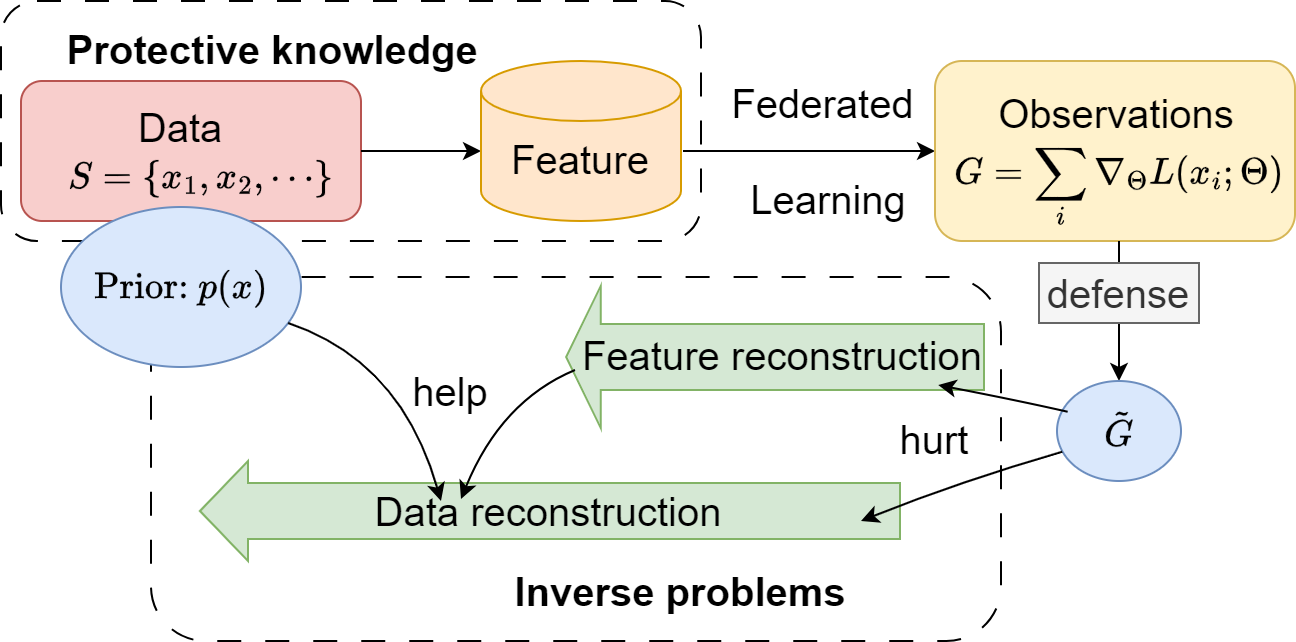
Figure 1: An illustration of the key components of data reconstruction studied in this paper.

Prior data reconstruction attacks have centered around gradient inversion (Zhu et al., 2019), attempting to match gradients generated from dummy and real input variables. Some variants in this line incorporate prior input data knowledge as regularization in the objective function (Jeon et al., 2021; Yin et al., 2021). As illustrated in Fig. 1, the reconstruction attack can be viewed as an inverse problem; from the observations $G$ that is generated from the unknown data and a known function (model’s gradient), the adversary intends to reconstruct the input data, and a defending method is to prevent this from perturbing the observations. To evaluate the effectiveness of a defense is to evaluate how robust it is to the strongest attack within the threat model.

However, previous attacks lack strength and theoretical guarantees, making the evaluation of the defense’s strength untrustworthy. Empirical understanding of attacking and defending methods is affected by factors like optimization challenges of non-convex objectives. Under the heuristic attacking methods from prior work, it is hard to disentangle the following two possibilities: 1) the algorithmic or computational barrier of the attack, and 2) the success of the defense. In this work, we will investigate the problem by introducing stronger attacks, as well as bringing more theoretical perspectives.

A line of theoretical work analyzing privacy attacks is differential privacy (DP) (Dwork, 2006), which guarantees privacy in data re-identification or membership inference. However, there are scenarios when data identity information is not sensitive but data itself is, and DP is not suitable to interpret data reconstruction attacks Guo et al. (2022). As a concrete example, when the observation $G$ is the sum of the samples, it yields no DP guarantee but recovering data from the sum is impossible as long as there are multiple data points. Although there are previous works discussed the reconstruction attack under differential privacy setting (Guo et al., 2022; Stock et al., 2022), their setting is different from federated learning where all samples but one are known and the goal of the attacker is to reconstruct the last data point, which is unrealistic in the federate learning setting. To this end, with DP not applicable in this setting, there is limited theoretical work and it is urgent to call for more fundamental investigations on the data reconstruction problems.

Recent work by Wang et al. (2023) introduced a theoretically sound feature reconstruction attack, but lacked practicality as it focused on two-layer fully connected neural networks, while for deep networks it had to manipulate the bottom layers’ weights in a transparently detectable way. We enhance this attack by combining gradient and intermediate layer matching, where we utilize the methodology in (Wang et al., 2023) as a pre-processing step of intermediate layer reconstruction. In the setting of an honest-but-curious server, our stronger attack demonstrates robustness to various defenses through empirical validation. Moreover, the robustness can be theoretically analyzed, differing from previous attacks. Under the framework of this attack, we can conduct a more systematic and scientific evaluation of privacy defenses’ utilities. Our main contributions are the following:

• We propose a new gradient inversion attack method. Leveraging the use of an untrained U-Net as an image prior and intermediate feature matching. The proposed method can recover data from gradients and be robust to a wide range of defense methods.

• We establish theoretical analyses to thoroughly evaluate the effectiveness of a wide range of common defense strategies against feature recovery, providing a theoretical perspective in reconstruction attack and defense.

• We further conduct extensive experiments on the common defense strategies with the proposed attack method, connecting theoretical principles with practice.

1.1 Related Work

In federated learning (Konečný et al., 2016; McMahan et al., 2017), a line of work in gradient inversion aims to reconstruct training data from gradients. An early work by Aono et al. (2017) theoretically showed that reconstruction is possible under a single neuron setting. Following this line, Zhu et al. (2019) proposed the gradient matching framework, where the training data and labels are recovered by minimizing the $l_{2}$ distance between gradients generated by dummy variables and real data. Instead of using $l_{2}$ distance, Wang et al. (2020) proposed a Gaussian kernel-based distance function, and Geiping et al. (2020) used cosine similarity.

Apart from using different distance measures, recent works introduced image priors to gradient matching. Geiping et al. (2020) added a total variation regularization term since pixels of a real image are usually similar to their neighbor. Wei et al. (2020a) introduced a label-based regularization to fit the prediction results. Balunovic et al. (2021) formulated the gradient inversion attack in a Bayesian framework. Yin et al. (2021) used a batch-normalization regularization to fit the BN statistics and a group consistency regularization to indicate the spatial equivariance of CNN. Instead of using regularization terms, Jeon et al. (2021) represented dummy training data by a generative model to preserve the image prior. In this method, the latent variables and the parameters of the generative model are trained simultaneously.

Some recent works investigated new data reconstruction methods outside the framework of gradient matching. Wang et al. (2023) theoretically showed that the training data can be reconstructed from gradients of networks with random weights using tensor decomposition methods, where optimization is not needed. Haim et al. (2022) proposed a reconstruction method using the stationary property for trained neural networks, induced by the implicit bias of training.

Defense strategies in this setting, however, are relatively less studied. The original setting of federated learning proposed by McMahan et al. (2017) used local aggregation to update multiple steps instead of gradients directly. Bonawitz et al. (2016, 2017) proposed a secure aggregation that can collect the gradients from multiple clients before updating. Geyer et al. (2017); Wei et al. (2020b) introduced differential privacy into federated learning, perturbing the gradients. Aono et al. (2017) demonstrated an encryption framework in the setting of federated learning. Moreover, many tricks designed to improve the performance of neural networks are effective in defending against privacy attacks, such as Dropout (Hinton et al., 2012), gradient pruning (Sun et al., 2017), and MixUp (Zhang et al., 2017). The effect of defending strategies against gradient matching attacks are discussed in (Zhu et al., 2019; Geiping et al., 2020; Huang et al., 2021).

2 A Stronger Attack for Defense Methods Evaluation

Prior research has demonstrated the potential to retrieve input directly from gradient values, specifically for image classification endeavors, by presenting it as an optimization problem: when provided with a neural network characterized by parameters $\theta$ and its associated gradient $\nabla_{\theta}\mathcal{L}(x^{\ast},y^{\ast})$ computed with a private data batch $(x^{\ast},y^{\ast})\in\mathbb{R}^{b\times d}\times\mathbb{R}^{d}$, $b$ is the batch size, $d$, for example, is the image size. Attack methods tries to recover $x$, an estimation of $x^{\ast}$:

$$\arg\min_{x}\mathcal{L}_{\rm grad}(x;\theta,\nabla_{\theta}\mathcal{L}_{\theta}(x^{*},y^{*}))+\alpha\mathcal{R}_{\rm aux}(x)$$ (1)

The optimization objective is twofold: the initial term $\mathcal{L}_{\rm grad}(x;\theta,\nabla_{\theta}\mathcal{L}_{\theta}(x^{\ast},y^{\ast}))$ ensures that the gradient of the retrieved batch $x$ aligns with the given gradients. Meanwhile, the regularization term $\mathcal{R}_{\rm aux}(x)$ refines the recovered image using established image prior(s) such as total variation. This is because Eq. (1) is non-convex, and inverting gradients is often under-determined, i.e. there exists a pair of different data having the same gradient even when the learning model is large.

Meanwhile, a recent work by Wang et al. (2023) introduced a novel tensor-based approach for reconstructing input data from the gradients of two-layer fully connected neural networks. Distinct from traditional optimization-based gradient matching techniques, this tensor-based strategy has been shown, both theoretically and empirically, to offer superior performance. In the pursuit of building a more robust attack method that enhances defense mechanisms evaluation. we explore the integration of this tensor-based methodology with existing optimization-based gradient matching approaches. Specifically, the tensor-based technique is applied to reconstruct intermediate features before the fully connected layers, which commonly serve as classification heads in modern neural network architectures. High-quality reconstruction of these features, as evidenced by (Wang et al., 2023), provides additional information that can be utilized to further regularize the objective equation Eq. (1), thereby making gradient matching more computationally tractable. As we demonstrated in Figure 2 and Table 1, introducing feature matching to gradient matching results in a more potent attack methodology. This integrated approach not only strengthens the attack but also facilitates a more comprehensive theoretical examination of various defense strategies.

2.1 Our attack algorithm

In this section, we present a stronger attack algorithm designed to rigorously evaluate various defense mechanisms. The method follows (Geiping et al., 2020) to use the same selection of $\mathcal{L}_{\rm grad}$ and research (Yin et al., 2021) for regularization grounded in batch normalization. A key innovation of our method is the integration of additional regularizations, inspired by the recent contributions of (Wang et al., 2023). This novel incorporation seeks to strength the attack strategy, ensuring a more precise and efficient evaluation of defense methods.

Feature reconstruction with tensor-based method

To utilize the feature matching regularization, we have to obtain the intermediate feature as a preprocessing step. Since the federated learning model cannot directly access the intermediate feature, a feature reconstruction with small errors is needed. The setting of recovering the intermediate feature is the same as reconstructing input data from the gradient of a fully connected 2-layer neural network. Specifically, we denote the input dimension by $d$ and the number of classes by $K$. For a two layer neural network $f({\bm{x}};\Theta)=\frac{1}{m}A\sigma(W{\bm{x}})$ with $m$ hidden nodes, where $W=[{\bm{w}}_{1},\dots,{\bm{w}}_{m}]\in\mathbb{R}^{m\times d}$, $A=[{\bm{a}}_{1},\dots,{\bm{a}}_{K}]^{\top}\in\mathbb{R}^{K\times m}$ and $\sigma$ is point-wise, denote $z_{k}=a_{k}^{\top}\sigma(W{\bm{x}})$ and $p_{k}=\mathrm{Softmax}(z_{k})$. Then with cross-entropy loss, for input ${\bm{x}}$ we can observe the partial derivative

$$\frac{\partial\ell}{\partial a_{kj}}=\frac{\partial\ell}{\partial z_{k}}\frac{\partial z_{k}}{\partial a_{kj}}=\frac{1}{m}(p_{k}-y_{k})\sigma({\bm{w}}_{j}^{\top}{\bm{x}})$$

from gradient. We adopt the tensor-based reconstruction method proposed by Wang et al. (2023). We can define $g({\bm{w}}_{j})=\sum_{k=1}^{K}c_{k}\frac{\partial\ell}{\partial a_{kj}}$, where $c_{k}$’s are some constant with carefully chosen such that $r_{i}:=\sum_{k=1}^{K}c_{k}(p_{ki}-y_{ki})$ is a constant. Then compute $\sum_{j=1}^{m}g({\bm{w}}_{j})H_{p}({\bm{w}}_{j}),$ where $H_{p}$ is the $p$-th Hermite function, and conduct tensor decomposition. See details of the method in Appendix B.

Strategic weight initialization.

In addressing the challenge of integrating a tensor-based method, which requires randomly initialized networks, into gradient inversion processes that typically see improved performance with a few steps of preliminary training, we have designed a strategic approach for weight initialization. Since tensor-based method is only applied to the final fully connected layers, denoted as $A\sigma(Wx)$, where $A\in\mathbb{R}^{K\times m},\;W\in\mathbb{R}^{m\times d}$, with $K$ representing the number of classes, $m$ the number of hidden nodes, and $d$ the input dimension. We consider the original pre-trained weights to be partitioned into two sets: $W=[W_{1},W_{2}]$ and $A=[A_{1};A_{2}]$. Here, $W_{2}\in\mathbb{R}^{v\times d}$ is initialized as a random Gaussian matrix, essential for the tensor-based method to function effectively. Concurrently, each row $i$ of $A_{2}\in\mathbb{R}^{K\times v}$ is initialized to a constant value of $i/v$, as suggested by the tensor-based approach. The remaining dimensions of the weight matrices, $W_{1}\in\mathbb{R}^{(m-v)\times d}$ and $A_{1}\in\mathbb{R}^{K\times(m-v)}$, retain their pre-trained weights, aligning with the requirements for successful gradient matching. For all of our experiments, the dimension allocated for gradient matching, $m-v$, is set as 2048. This strategic initialization approach not only accommodates the prerequisites of the tensor-based method but also maintains the efficacy of the gradient-matching process.

Challenges in order recovery of the features.

When deploying the tensor-based method for feature recovery, a challenge arises due to the algorithm’s inability to precisely maintain the order and sign of features when dealing with batches larger than a single input. This challenge complicates the task of accurately matching the recovered features to their corresponding inputs within a batch. In theory, one approach to circumvent this issue is to consider every possible permutation of the recovered features against the batch inputs, aiming to identify the correct alignment. However, this method is computationally intensive and impractical for larger batches. To streamline the process, we adopt a more efficient strategy that involves sequentially comparing each recovered feature against the actual input features using cosine similarity. This comparison continues until the most accurate order of features is determined based on their similarity scores. Although a single recovered feature might have high cosine similarity with several features corresponding to different inputs, we empirically observe that this greedy matching method achieves similar performance with the method that considers all possible pairs.

Regularization on feature matching.

To address the challenge of non-unique solutions in gradient matching, we introduce a regularization term designed to align intermediate network features with those reconstructed via a tensor-based method. This regularization, denoted as $\mathcal{R}_{\text{feature}}(x)$, employs squared cosine similarity to mitigate the issue of sign ambiguity inherent in tensor-based reconstruction:

$$\mathcal{R}_{\rm feature}({x})=1-\left(\frac{\langle f({x},\phi),\hat{z}\rangle}{\left\|f({x},\phi)\right\|\left\|\hat{z}\right\|}\right)^{2},$$ (2)

where $f(x,\phi)$ are the intermediate features of input $x$ and $\hat{z}$ are the reconstructed features from the tensor-based method. This approach aims to refine gradient matching by ensuring the generated input $x$ yields intermediate features similar to $\hat{z}$, providing a more accurate and specific solution space.

Other regularizations.

Following  (Geiping et al., 2020), we adopt total variation and regularization on batch norm to exploit prior knowledge of natural images and training data. Moreover, inspired by deep image prior (Ulyanov et al., 2018), we employ an untrained Convolutional Neural Network (CNN) to generate an image. This idea is rather similar to (Jeon et al., 2021) where a network is pre-trained for image generation. The final objective of the introduced attack method is

$$\arg\min_{x} \mathcal{L}_{\rm grad}(x;\theta,\nabla_{\theta}\mathcal{L}_{\theta}(x^{*},y^{*}))+\alpha_{TV}\mathcal{R}_{\rm TV}+\alpha_{BN}\mathcal{R}_{\rm BN}+\alpha_{f}\mathcal{R}_{\rm feature}(x).$$ (3)

3 Defense Methods

To combat privacy attacks of machine learning, some defenses are proposed to prevent data leakage. Specifically in the setting of data reconstruction attack in federated learning, (Zhu et al., 2019; Geiping et al., 2020; Huang et al., 2021) evaluated the privacy of different defending strategies empirically. These works shed light on choosing appropriate defenses against reconstruction attacks but can be improved in the following sense: (i) the attacks they used to evaluate defenses lack strength. However, the definition of how robust a defense strategy is should be measured on the strongest attack within the threat model; and (ii) previous evaluations are purely empirical without theoretical support. In contrast, our evaluation of defenses is based on a stronger attack we proposed. Moreover, we also provide theoretical analysis from the perspective of feature reconstruction.

Our attack is composed of gradient matching and feature matching. Defenses bring both optimization and statistical barriers to the gradient matching component, where the effect is difficult to analyze theoretically. The feature-matching component, on the other hand, can be analyzed quantitatively. The quality of feature matching is not only essential to and correlates strongly with the overall performance of data reconstruction, but the intermediate feature, as well as original data, is also protective information and its leakage should be prevented as well. To this end, we will theoretically analyze the defending effect on feature reconstruction in the following part of this section.

With our stronger attack, the feature reconstruction is equivalent to recovering the input of a two-layer neural network. Thus, our theoretical analysis can be based on the results of reconstruction error bounds on two-layer networks in (Wang et al., 2023) but varies among different defenses. On one hand, our theoretical findings overturned some prior empirical observations on the effectiveness of several defense methods. On the other hand, it is generally more convincing to analyze the effect of defenses under a stronger and more robust attacking method. Combined with the experiments in Section 4, our analysis gives a more complete understanding of various defending methods.

In the following analysis, our setting conforms to that of Section 2.1 with a main focus on feature reconstruction of fully connected layers.

3.1 No defense

Without any defense, we conduct tensor decomposition to $\sum_{j=1}^{m}g({\bm{w}}_{j})H_{p}({\bm{w}}_{j})$ as stated in Section 2.1. Then by the following Stein’s lemma (Stein, 1981; Mamis, 2022):

Lemma 3.1 (Stein’s Lemma).

Let $X$ be a standard normal random variable. Then for any function $g$, we have

$$\mathbb{E}[g(X)H_{p}(X)]=\mathbb{E}[g^{(p)}(X)],$$ (4)

if both sides of the equation exist. Here $H_{p}$ is the $p$th Hermite function and $g^{(p)}$ is the $p$th derivative of $g$.

we have

$$\sum_{j=1}^{m}g({\bm{w}}_{j})H_{p}({\bm{w}}_{j})\approx m\operatorname{\mathbb{E}}_{{\bm{w}}\sim\mathcal{N}(0,I)}[g({\bm{w}})H_{p}({\bm{w}})]$$

$$=m\operatorname{\mathbb{E}}_{\bm{w}}[\nabla^{p}_{\bm{w}}g({\bm{w}})]= \sum_{i=1}^{B}r_{i}\mathbb{E}[\sigma^{(p)}({\bm{w}}^{\top}{\bm{x}}_{i}){\bm{x}}_{i}^{\otimes p}].$$ (5)

Thus, the result of tensor decomposition is $\{x_{1},\dots,x_{B}\}$ and the error bound is $\tilde{O}(BK\sqrt{\frac{d}{m}})$ with high probability, where $B$ is the batch size of data. Details of the analysis is in Appendix B.

3.2 Local aggregation

In a realistic setting of federated learning, the observed local update may not be a single gradient. Instead, it can be the result of multiple steps of gradient descent. Specifically, under the setting of federated averaging (McMahan et al., 2017), a client with $N$ images trains $E$ epochs for each update, where a single epoch contains $N/B$ gradient descent steps with batch size $B$.

Since the observation is more complicated than a gradient, the difficulty of reconstructing features increases. However, the tensor-based attack can still work under this setting. For an update $\tilde{g}$ with multiple steps, we can simply replace the gradient $g$ in the previous attack with $\tilde{g}$ and conduct tensor decomposition as normal. Specifically, we will discuss two cases: using the same batch to train multiple steps and using different batches for every gradient step.

Multiple steps with the same batch.

In this setting, $B=N$ and $E>1$. We first consider the case $E=2$. According to gradient descent, we have $a_{kj}^{(t+1)}=a_{kj}^{(t)}-\frac{\eta}{m}\sum_{i=1}^{B}(p_{ki}^{(t)}-y_{ki}^{(t)})\sigma({\bm{w}}_{j}^{(t)}\cdot{\bm{x}}_{i})$ for $t=0,1$, where $p_{ki}^{(t)},y_{ki}^{(t)},a_{kj}^{(t)},{\bm{w}}_{j}^{(t)}$ are the values of corresponding parameters after $t$ gradient steps. Since the information from clients are the values of $a_{j}^{(2)}$, we have from the local update

$$\begin{split}a_{kj}^{(2)}-a_{kj}^{(0)}=-\frac{\eta}{m}\sum_{i=1}^{B}(p_{ki}^{(0)}-y_{ki}^{(0)})\sigma({\bm{w}}_{j}^{(0)}\cdot{\bm{x}}_{i})-\frac{\eta}{m}\sum_{i=1}^{B}(p_{ki}^{(1)}-y_{ki}^{(1)})\sigma({\bm{w}}_{j}^{(1)}\cdot{\bm{x}}_{i}).\end{split}$$ (6)

Under this setting, we can compute $\sum_{j=1}^{m}\sum_{k=1}^{K}c_{k}(a_{kj}^{(2)}-a_{kj}^{(0)})H_{p}({\bm{w}}_{j})$ and conduct rank-$B$ tensor decomposition, which is similar to the original problem. For the attack, we can prove that the reconstruction error is bounded by $\tilde{O}(BK\sqrt{\frac{d}{m}})$ with high probability.

Different batches.

In this setting, $E=1$ but $N>B$. We first consider the case with only 2 batches, i.e. $B<N\leq 2B$. Similar to Eq.(6), the local update

$$\begin{split}a_{kj}^{(2)}-a_{kj}^{(0)}=&-\eta\sum_{i=1}^{B}(p_{ki}^{(0)}-y_{ki}^{(0)})\sigma({\bm{w}}_{j}^{\top}{\bm{x}}_{i})-\eta\sum_{i=B+1}^{N}(p_{ki}^{(1)}-y_{ki}^{(1)})\sigma({\bm{w}}_{j}^{(1)}\cdot{\bm{x}}_{i}).\end{split}$$ (7)

The only difference from the case above is that the data used to train $\Theta^{(1)}$ is different from the one in training $\Theta^{(0)}$. Thus, performing our attacking method with $N$ outputs instead of $B$ can reconstruct the original data. We can prove that the reconstruction error is bounded by $\tilde{O}(NK\sqrt{\frac{d}{m}})$ with high probability.

Conclusion.

Note that for both cases, if there are more than 2 gradient steps, we can perform the same tensor decomposition method. Thus, the tensor-based attack can recover features against local aggregation attacks. The proofs of the error bounds above are in Appendix C.1.

3.3 Differential privacy stochastic gradient descent

Differential privacy (Dwork, 2006) algorithms ensure the privacy of data by adding noise to gradient descent steps (Shokri and Shmatikov, 2015; Abadi et al., 2016; Song et al., 2013). In this way, it hides the exact local gradient from the global model. In differential private federated learning (Geyer et al., 2017; Wei et al., 2020b), each client clips the gradient and introduces a random Gaussian noise before updates to the cluster. In the setting of two-layer networks, the update of $a_{j}$ is

$$\tilde{g}_{j}=g_{j}/\max\left\{1,\frac{\|g\|}{S}\right\}+\epsilon,\text{ where }\epsilon\sim\mathcal{N}(0,\sigma^{2}I).$$

Note that under this setting, the information contained in the gradient is disrupted by gradient clipping and random noise. We first analyze the effect of the two strategies separately. For gradient clipping, we conduct our method based on observed clipped gradient $\tilde{g}$. There will be no defensive effect to our attack no matter the clipping threshold and we can prove that the reconstruction error bound $\tilde{O}(BK\sqrt{\frac{d}{m}})$ is the same as that with no defense (even for the hidden terms). For noisy gradient $g+\epsilon$, we have the same order of error bound if the noise level $\sigma\leq O(\frac{B}{m})$ so the defense is not effective.

In the defense of differential privacy gradient descent, we combine the two strategies and conduct a tensor method based on $\tilde{g}+\epsilon$. The defense is more effective and has an error bound $O(\max\{1,\frac{\|g\|}{S}\})$ times to the bound of gradient noise defense only. Gradient clipping enhances the defensive performance of the gradient noise though itself has no effect in defending the attack. However, our attack method is still enough to recover the feature since we can modify the initial weights to control $\|g\|$.

Conclusion.

The defense of gradient clipping has no effect while gradient noise and differential privacy gradient descent is successful only when the noise level is relatively large. However, the noise variance $\sigma^{2}$ in the application is usually small since a large random noise will cause bad performance in federated learning (Wei et al., 2020b). We also show some results in Section 4. See detailed proofs of the error bounds in Appendix C.2.

3.4 Secure aggregation

In federated learning, local devices update gradients to the server individually. Secure aggregation (Bonawitz et al., 2016, 2017) is a method that clients $\{u_{1},\dots,u_{L}\}$ can aggregate their gradients prior to the cluster and the cluster can only access to aggregated gradient: $\tilde{G}=\frac{1}{B}\sum_{i=1}^{L}g_{l}B_{l},$ where $g_{l}$ and $B_{l}$ is the gradient update and batch size for user $u_{l}$ respectively and $B=\sum_{i=1}^{L}B_{l}$. In this way, the global server is blocked from knowing each individual gradient and then prevents privacy leakage. Even though the server can reconstruct the training data, it cannot identify which user has the data. If we only reconstruct data without identifying its source, the aggregated gradient is equivalent to a gradient step with large batch size $B$ and we can conduct our tensor-based attack on the aggregated gradient.

Conclusion.

Tensor method will still work when the batch size is not too large. Otherwise, say $B>d$, feature recovery cannot work since the tensor decomposition is not unique.

3.5 Dropout

Another method to improve the defending effect is dropout (Hinton et al., 2012; Srivastava et al., 2014), which is a mechanism designed to prevent overfitting. It randomly drops nodes in a network with a certain probability $1-p$. In this way, some of the entries in the gradient randomly turn to zero. Since dropout introduces randomness to the gradient, it can be used to defend against privacy attacks in federated learning. The effect of dropout against gradient matching is empirically discussed in (Zhu et al., 2019; Huang et al., 2021). A two-layer fully connected network with a dropout layer can be written as

$$f({\bm{x}};\Theta)=\sum_{j=1}^{m}s_{j}a_{j}\sigma({\bm{w}}_{j}\cdot{\bm{x}})=\sum_{j:s_{j}=1}a_{j}\sigma({\bm{w}}_{j}\cdot{\bm{x}}),$$

where $s_{j}\sim\mathrm{Bernoulli}(p)$. Thus, the model has an effective width equal to the number of nodes $m^{\prime}$ that has not been dropped. We can compute the sum $\frac{1}{m^{\prime}}\sum_{j:s_{j}=1}g_{j}H_{p}({\bm{w}}_{j})$ and conduct tensor decomposition. Since the effective width $m^{\prime}\approx pm$, the defense is not effective when $p$ is not too small.

3.6 Gradient pruning

Gradient pruning (Sun et al., 2017; Ye et al., 2020) is a method that accelerates the computation in training by setting the small entries in gradient to zero. Thus, the gradient will be sparse, which is similar to dropout. However, the key difference is that the remaining entries of the gradient in dropout are chosen randomly yet gradient pruning drops small entries making the defending more effective (when a similar level of utility is lost).

If we denote the set of entries that is not pruned by $S$ and conduct the tensor-based attack, we have

$$\hat{{\bm{T}}}_{p}=\frac{1}{m^{\prime}}\sum_{j\in S}g_{j}H_{p}({\bm{w}}_{j}),$$

where $g_{j}=\nabla_{a_{j}}L$ and $m^{\prime}=|S|$. This formula has a similar form to the case in dropout but the key difference is that the remaining ${\bm{w}}_{j}$’s are more likely to make $g_{j}$ larger so they do not follow the normal distribution. In this case, the concentration property $\sum_{j\in S}g({\bm{w}}_{j})H_{p}({\bm{w}}_{j})\approx m^{\prime}\operatorname{\mathbb{E}}_{{\bm{w}}\sim\mathcal{N}(0,I)}[g({\bm{w}})H_{p}({\bm{w}})]$ may not hold. Moreover, Lemma 3.1 cannot be applied with ${\bm{w}}_{j}$’s are not normal random vectors so $\operatorname{\mathbb{E}}_{{\bm{w}}\sim\mathcal{N}(0,I)}[g({\bm{w}})H_{p}({\bm{w}})]\neq\operatorname{\mathbb{E}}_{\bm{w}}[\nabla^{p}_{\bm{w}}g({\bm{w}})]$. Thus, the $\hat{{\bm{T}}}_{p}$ is not a good estimation of the real tensor product, indicating gradient pruning defense is effective against feature reconstruction.

4 Experiments

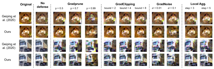
Figure 2: Comparison of the reconstruction results from the gradient inversion method (Geiping et al., 2020) and our proposed attack method on different defenses with batch size equal to 4. Our method achieves more robust reconstruction across various defenses. Gradient pruning ($p=0.99$) makes reconstructions from both methods almost unrecognizable.

Batch Size	16			32
Method	Geiping	Jeon	Ours	Geiping	Jeon	Ours
LPIPS $\downarrow$	0.41 (0.09)	0.17 (0.12)	0.14 (0.11)	0.45 (0.11)	0.24 (0.13)	0.15 (0.11)

Table 1: Comparison of our methods with other state-of-the-art methods, Geiping, and Jeon refer to (Geiping et al., 2020) and (Jeon et al., 2021) respectively. We highlight the best performances in bold.

4.1 Experimental setup

Key parameters of defenses.

We evaluate defense methods on CIFAR-10 dataset (Krizhevsky et al., 2009) with a ResNet-18 (trained for one epoch), which is the default backbone model for federated learning. For the deep image prior model, we use a U-Net backbone similar to an unmasked PixelCNN++ (Salimans et al., 2017; Ronneberger et al., 2015) and replace the original weight normalization (Salimans and Kingma, 2016) with group normalization (Wu and He, 2018). We use self-attention at the $16\times 16$ feature map resolution (Wang et al., 2018). The details are in the Appendix D. For GradPrune: gradient pruning sets gradients of small magnitudes to zero. We vary the pruning ratio $p$ in $\{0.3,0.5,0.7,0.9,0.99\}$. For GradClipping: gradient clipping set gradient to have a bounded norm, which is ensured by applying a clipping operation that shrinks individual model gradients when their norm exceeds a given threshold. We set this threshold as $\{2,4,8\}$. We also adopt defense by adding noise to gradient, the noise is generated from random Gaussian with different standard deviations $\{0.001,0.01,0.05,0.1\}$. Local gradient aggregation aggregates local gradient by performing a few steps of gradient descent to update the model. We locally aggregate $3$ or $5$ steps.

Key experimental setup for the attack.

We use a subset of 50 CIFAR-10 images to evaluate the attack performance. To achieve a strong attack, we add reconstructed features (after linear projections to match the dimension) into each residual block of the U-Net. We also assume the batch norm statistics are available following (Geiping et al., 2020). We observe the difficulty of optimization when using cosine-similarity as the gradient inversion loss under our setting, and therefore address this issue by reweighting the gradients by their $\ell_{0}$ norm. See details in the Appendix D. Geiping et al. (2020); Zhu et al. (2019) have shown that small batch size is vital for the success of the attack. We intentionally evaluate the attack with two small batch sizes $4$ and $8$ and two small but realistic batch sizes, 16 and 32.

Metrics for reconstruction quality.

We visualize reconstructions obtained under different defenses. Following (Yin et al., 2021), we also use the RMSE, PSNR, and learned perceptual image patch similarity (LPIPS) score (Zhang et al., 2018) to measure the mismatch between reconstruction and original images. For the evaluation of feature reconstruction, we use the average norm of projection from original features to the orthogonal complement of the space spanned by reconstructed features. This metric measures the difference between the two spaces spanned by original and reconstructed features. Compared with the average cosine similarity between features, this metric is more robust when some features are similar.

4.2 Experiment results

Results of the proposed attack method.

Our method can be easily added to previous methods (Geiping et al., 2020; Zhu et al., 2019). In Table  1, we compare the state-of-the-art methods with the proposed attacking method, our method outperforms previous methods. We visualize reconstructed images in Figure 2. Without any defense, both (Geiping et al., 2020) and our attack method can recover images well from the gradient, and our method produces higher-quality images. Increasing the batch size makes all methods more difficult to recover well. With defenses, our method shows better robustness – the recovered images are visually similar to the original image. This result shows that our attack is a stronger attack under these defense methods. Figure 3(b) suggests that the feature matching loss is the main reason behind such robustness, showing that the analysis of feature reconstruction is reasonable. See Table 3 and Table 5 in Appendix E for summary of reconstruction results.

			Gradprune			GradClipping			GradNoise		Local Aggregation
Batchsize	w/o defense	p=0.3	p=0.5	p=0.7	bound=2	bound=4	bound=8	0.001	0.01	0.1	step=3	step=5
1	0.171	0.173 (0.002)	0.173 (0.002)	0.248 (0.006)	0.173 (0.002)	0.173 (0.002)	0.173 (0.002)	0.172 (0.003)	0.174 (0.002)	0.259 (0.012)	0.181 (0.067)	0.213 (0.071)
2	0.171	0.171 (0.003)	0.218 (0.011)	0.443 (0.120)	0.169 (0.003)	0.169 (0.003)	0.170 (0.003)	0.166 (0.003)	0.252 (0.082)	0.850 (0.108)	0.186 (0.127)	0.210 (0.087)
4	0.174	0.186 (0.114)	0.277 (0.106)	0.483 (0.075)	0.174 (0.116)	0.175 (0.127)	0.177 (0.113)	0.190 (0.021)	0.252 (0.106)	0.714 (0.102)	0.192 (0.079)	0.218 (0.081)
8	0.175	0.188 (0.044)	0.266 (0.071)	0.425 (0.043)	0.179 (0.041)	0.179 (0.041)	0.179 (0.041)	0.198 (0.114)	0.499 (0.104)	0.953 (0.108)	0.202 (0.073)	0.223 (0.069)

Table 2: Feature reconstruct error under different defenses. When using gradient pruning defense and gradient noise defense with large $\sigma$, the feature reconstruction quality degrades significantly.

	None	GradNoise ($\sigma$)				GradPrune ($p$)					GradClipping (bound)			Local Aggregation (step)
Parameter	-	0.001	0.01	0.05	0.1	0.3	0.5	0.7	0.9	0.99	2	4	8	3	5
Attack batch size $=2$
RMSE $\downarrow$	0.15(0.04)	0.17 (0.05)	0.22 (0.07)	0.31 (0.06)	0.28 (0.08)	0.16 (0.08)	0.17 (0.07)	0.20 (0.09)	0.26 (0.09)	0.27 (0.10)	0.17 (0.08)	0.17 (0.08)	0.19 (0.08)	0.23 (0.09)	0.25 (0.10)
PSNR $\uparrow$	23.69 (5.69)	23.31 (3.04)	21.32 (3.52)	14.58 (1.59)	13.11 (4.26)	22.63 (6.15)	23.33 (6.03)	19.40 (6.02)	16.39 (6.56)	14.72 (6.45)	23.26 (6.10)	23.40 (6.00)	23.01 (6.28)	18.65 (6.75)	18.77 (7.33)
Attack batch size $=4$
RMSE $\downarrow$	0.15 (0.03)	0.19 (0.07)	0.24 (0.08)	0.29 (0.03)	0.27 (0.07)	0.16 (0.04)	0.16 (0.03)	0.21 (0.04)	0.27 (0.07)	0.27 (0.08)	0.16 (0.03)	0.16 (0.04)	0.16 (0.04)	0.28 (0.08)	0.26 (0.08)
PSNR $\uparrow$	23.59 (5.39)	20.12 (3.58)	16.41 (4.64)	11.27 (0.33)	12.28 (4.08)	23.16 (5.48)	24.08 (5.38)	18.73 (5.63)	13.90 (3.77)	12.43 (2.73)	22.88 (5.31)	23.93 (5.55)	24.04 (5.58)	13.84 (5.38)	14.21 (5.41)
Attack batch size $=8$
RMSE $\downarrow$	0.15 (0.04)	0.19 (0.05)	0.29 (0.05)	0.30 (0.03)	0.30 (0.06)	0.15 (0.03)	0.16 (0.04)	0.20 (0.05)	0.29 (0.05)	0.29 (0.05)	0.16 (0.03)	0.16 (0.04)	0.16 (0.04)	0.29 (0.04)	0.30 (0.04)
PSNR $\uparrow$	23.37 (5.42)	20.31 (4.13)	14.56 (0.88)	11.27 (0.89)	11.27 (1.83)	23.74 (5.21)	23.32 (5.13)	18.25 (5.22)	11.30 (2.10)	11.13 (2.15)	23.36 (5.14)	23.59 (5.41)	23.47 (5.23)	11.25 (2.56)	10.82 (2.20)

Table 3: Our method evaluated with different defense methods. With feature matching, our method performs well against most defenses. Specifically, gradient pruning shows its effectiveness under this stronger attack as well.

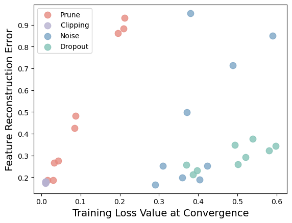
(a) Feature reconstruction error vs final training loss.

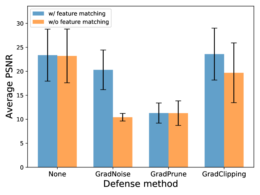
(b) PSNR of our method against different defenses.

Figure 3: The results of defenses against our attack. (a) The final training loss measures the level of interference with the training of defenses. The relation between feature error and interference reflects the effect of defenses. (b) PSNR of reconstructed data using the method with and without feature matching. The difference indicates that feature matching improves robustness against defenses.

Comparison of defense methods in feature recovery.

For feature recovery, we compared the reconstruction error under different defending strategies, and the results are shown in Table 2. We also use the final training loss of the federated learning model to measure the level of interference from defenses toward the training (details see Table 6 in Appendix E). For an effective defense, it should increase the feature reconstruction error while disturbing little to the training. We show the relation between reconstruction error and final training loss with different defenses in Figure 3(a). Gradient pruning has a large reconstruction error without increasing training loss too much so it has the best defending effect under this criteria. Adding noise also prevents feature leakage when noise is large enough but it will affect training. Gradient clipping is barely effective for defending feature recovery while dropout has a mild effect but it is harmful to training. The feature reconstruction errors are consistent with the theoretical analysis in Section 3.

Comparison of defense methods in inputs reconstruction.

According to 3, data reconstructed by our method with defense gradient pruning and gradient noise has the smallest average PSNR, indicating that these two defenses are effective against our attack. However, according to Figure 3(a), the final training loss of gradient pruning is smaller than that of gradient noise even when the pruning parameter $p$ is very large. Therefore, gradient pruning is the best defense that prevents data leakage and maintains training utility at the same time. It is also shown in Figure 2 that gradient pruning with $p=0.9$ has the best defensive effect. Gradient noise with $\sigma=0.1$ also works but the final training loss is large, showing its interference towards training.

We also compared between our attack method and the method without feature matching against different defenses in Figure 3(b) to show the effect of feature matching. Here we choose the batch size $B=8$ and defenses gradient noise with $\sigma=0.001$, gradient pruning with $p=0.9$, and gradient clipping with threshold 4. It is shown that feature matching improves the robustness of our attack against gradient noise and gradient clipping defenses. This can be explained by our analysis in Section 3 that feature recovery works badly against gradient pruning and feature matching regularization has no effect with inaccurate features. See the quantified effect of defenses with and without feature matching in Table 3 and Table 5 in Appendix E.

5 Conclusion

In this paper, we conduct a systematic evaluation of various defense methods both theoretically and empirically. To perform the evaluation, we introduce a stronger attack method that is robust to a wide range of defense methods in the setting of honest-but-curious server. The method enhances the conventional gradient inversion attack by combining it with the feature reconstruction attack, where a tensor-based attack method is adopted. Our theoretical and empirical findings indicate that gradient pruning is the most effective defense method among many others, including gradient clipping, dropout, adding noise, local aggregation, etc.

Appendix A Preliminaries for Theoretical Analysis

A.1 Tensor Method

Various of noisy tensor decomposition can be used in tensor based attack (Wang et al., 2023). We select the method proposed by (Zhong et al., 2017) in our theoretical analysis since it can provably achieve a relatively small error with least assumptions.

Assumption A.1.

We make the following assumptions:

• Data: Let data matrix $X:=[{\bm{x}}_{1},\cdots,{\bm{x}}_{B}]\in\mathbb{R}^{d\times B}$, we denote the $B$-th singular value by $\pi_{\min}>0$. Training samples are normalized: $\|{\bm{x}}_{i}\|=1,\forall i\in[B]$.

• Activation: $\sigma$ is 1-Lipschitz and $\operatorname{\mathbb{E}}_{z\sim\mathcal{N}(0,1)}[\sigma^{\prime\prime}(z)]<\infty$. Let

  $$k_{2}=\min\{k\geq 2:|\operatorname{\mathbb{E}}_{z\sim\mathcal{N}(0,1)}[\sigma^{(k)}(z)]|\neq 0\}$$

  and

  $$k_{3}=\min\{k\geq 3:|\operatorname{\mathbb{E}}_{z\sim\mathcal{N}(0,1)}[\sigma^{(k)}(z)]|\neq 0\}.$$

  Then $\nu=|\operatorname{\mathbb{E}}_{z\sim\mathcal{N}(0,1)}[\sigma^{(k_{2})}(z)]|$ and $\lambda=|\operatorname{\mathbb{E}}_{z\sim\mathcal{N}(0,1)}[\sigma^{(k_{3})}(z)]|$ are not zero. We assume $k_{2}\leq 3$ and $k_{3}\leq 4.$.

We first introduce the method in (Zhong et al., 2017) when the activation function satisfies $k_{2}=2$ and $k_{3}=3.$ In addition to $\hat{{\bm{T}}}=\sum_{j=1}^{m}g({\bm{w}}_{j})H_{3}({\bm{w}}_{j})$, we also need the matrix $\hat{P}=\sum_{j=1}^{m}g({\bm{w}}_{j})H_{2}({\bm{w}}_{j})$ in the tensor decomposition, where $H_{p}$ is the $p$-th Hermite function. We first conduct the power method to $\hat{P}$ to estimate the orthogonal span $U$ of training samples ${\bm{x}}_{1},\dots,{\bm{x}}_{B}$ and denote it by $V$, where $V\in\mathbb{R}^{B\times d}$ is an orthogonal matrix. Then we conduct tensor decomposition with $\hat{{\bm{T}}}(V,V,V)$ instead of $T$ and have the estimation of $\{V^{\top}{\bm{x}}_{i}\}_{i=1}^{B}$. By multiplying column orthogonal matrix $V$, we can reconstruct training data. The advantage of this method is that the dimension of $\hat{{\bm{T}}}(V,V,V)$ is $B<d$. Then the error will depend on $B$ instead of $d$.

For activation functions such that $k_{2}=3$, we define $\hat{P}=\sum_{j=1}^{m}g({\bm{w}}_{j})H_{3}({\bm{w}}_{j})(I,I,{\bm{a}})$ and for activation functions such that $k_{3}=4$, we define $\hat{{\bm{T}}}=\sum_{j=1}^{m}g({\bm{w}}_{j})H_{4}({\bm{w}}_{j})(I,I,I,{\bm{a}})$, where ${\bm{a}}$ is any unit vector. In the proofs below, we only consider the case $k_{2}=2$ and $k_{3}=3$ while the proofs of other settings are similar.

Note that with this method only, we cannot identify the norm of recovered samples without the assumption of $\|{\bm{x}}_{i}\|=1$ for all $i$. However, in our stronger reconstruction attack, the feature matching term is the cosine similarity between the reconstructed feature and the dummy feature, where knowing the norm is not necessary. Thus, our assumption on $\|bx_{i}\|=1$ is reasonable and can simplify the method and the proof.

A.2 Error Bound

For the noisy tensor decomposition introduced above, we have the following error bound:

Theorem A.1 (Adapted from the proof of Theorem 5.6 in (Zhong et al., 2017).).

Consider matrix $\hat{P}=P+S$ and tensor $\hat{{\bm{T}}}={\bm{T}}+{\bm{E}}$ with rank-$B$ decomposition

$$P=\sum_{i=1}^{B}\nu_{i}{\bm{x}}_{i}{\bm{x}}_{i}^{\top},\ {\bm{T}}=\sum_{i=1}^{B}\lambda_{i}{\bm{x}}_{i}^{\otimes 3},$$

where ${\bm{x}}_{i}\in\mathbb{R}^{d}$ satisfying Assumption A.1. Let $V$ be the output of Algorithm 3 in (Zhong et al., 2017) with input $P$ and $\{s_{i}{\bm{u}}_{i}\}_{i=1}^{B}$ be the output of Algorithm 1 in (Kuleshov et al., 2015) with input ${\bm{T}}(V,V,V)$, where $\{s_{i}\}$ are unknown signs. Suppose the perturbations satisfy

$$\|S\|\leq\mu\leq O(\nu_{\min}\pi_{\min}),\ \|{\bm{E}}(V,V,V)\|\leq\gamma.$$

Let $N=\Theta(\log\frac{1}{\epsilon})$ be the iteration numbers of Algorithm 3 in (Zhong et al., 2017), where $\epsilon=\frac{\mu}{\nu_{\min}}$. Then with high probability, we have

$$\left\|{\bm{x}}_{i}-s_{i}V{\bm{u}}_{i}\right\|\leq\tilde{O}(\frac{\mu}{\nu_{\min}\pi_{\min}})+\tilde{O}(\frac{\kappa\gamma\sqrt{B}}{\lambda_{\min}\pi_{\min}^{2}}),$$

where $\kappa=\frac{\lambda_{\max}}{\lambda_{\min}}.$

With Theorem A.1, we only need to bound the error $\|P-\hat{P}\|$ and $\|{\bm{T}}-\hat{{\bm{T}}}\|$, where the bound varies under different settings. Wang et al. (2023) proved the error bound under the square loss setting. In the following section, we will propose error bounds with cross-entropy loss, which is more widely used in classification problems. We will also give error bounds when defending strategies are used against privacy attacks.

A.3 Matrix Bernstein’s Inequality

The following lemma is crucial to the concentration bounds $\|P-\hat{P}\|$ and $\|{\bm{T}}-\hat{{\bm{T}}}\|$.

Lemma A.2 (Matrix Bernstein for unbounded matrices; adapted from Lemma B.7 in (Zhong et al., 2017)).

Let $\mathcal{Z}$ denote a distribution over $\mathbb{R}^{d_{1}\times d_{2}}$. Let $d=d_{1}+d_{2}$. Let $Z_{1},Z_{2},\cdots,Z_{m}$ be i.i.d. random matrices sampled from $\mathcal{Z}$. Let $\bar{Z}=\mathbb{E}_{Z\sim\mathcal{Z}}[Z]$ and $\widehat{Z}=\frac{1}{m}\sum_{i=1}^{m}Z_{i}$. For parameters $\delta_{0}\in(0,1),M=M(\delta_{0},m)\geq 0,\nu>0,L>0$, if the distribution $\mathcal{B}$ satisfies the following four properties,

$$(I) \quad\mathbb{P}_{Z\sim\mathcal{Z}}\left\{\|Z\|\leq M\right\}\geq 1-\frac{\delta_{0}}{m}$$

$$(II) \quad\max\left(\left\|\underset{Z\sim\mathcal{Z}}{\mathbb{E}}\left[ZZ^{\top}\right]\right\|,\left\|\underset{Z\sim\mathcal{Z}}{\mathbb{E}}\left[Z^{\top}Z\right]\right\|\right)\leq\nu$$

$$(III) \quad\max_{\|{\bm{a}}\|=\|\bm{b}\|=1}\left(\underset{Z\sim\mathcal{Z}}{\mathbb{E}}\left[\left({\bm{a}}^{\top}Z\bm{b}\right)^{2}\right]\right)^{1/2}\leq L$$

Then we have for any $0<\delta_{1}<1$, if $\delta_{1}\leq\frac{1}{d}$ and $m\gtrsim M\log(1/\delta_{1})$, with probability at least $1-\delta_{1}-\delta_{0}$,

$$\|\widehat{Z}-\bar{Z}\|\lesssim\sqrt{\frac{\log(1/\delta_{1})(\nu+\|\bar{Z}\|^{2}+M+\delta_{0}L^{2})}{m}}$$

Appendix B Analysis of Feature Reconstruction

Wang et al. (2023) proposed a privacy attack based on tensor decomposition but they only analyzed the case of square loss. However, in classification problems, cross-entropy loss is widely used. Here we propose a conduct feature reconstruction method with tensor decomposition under cross-entropy loss setting, which is the detailed version of the method proposed in Section 2.1.

We define the network the same as Section 2.1. Let the input dimension be $d$ and the number of classes is $K$. For a two layer neural network $f({\bm{x}};\Theta)=\frac{1}{m}A\sigma(W{\bm{x}})$ with $m$ hidden nodes, where $W=[{\bm{w}}_{1},\dots,{\bm{w}}_{m}]\in\mathbb{R}^{m\times d}$, $A=[{\bm{a}}_{1},\dots,{\bm{a}}_{K}]^{\top}\in\mathbb{R}^{K\times m}$ and $\sigma$ is point-wise. Denote $z_{k}=a_{k}^{\top}\sigma(W{\bm{x}})$ and $p_{k}=\mathrm{Softmax}(z_{k})$. Then cross entropy loss is $\ell(f({\bm{x}};\Theta),{\bm{y}})=-\sum_{k=1}^{K}y_{k}\log(p_{k})$, where ${\bm{y}}\in\mathbb{R}^{K}$ is a one-hot vector. Then we have the gradient

$$\frac{\partial\ell}{\partial{\bm{w}}_{j}}=\sum_{k=1}^{K}\frac{\partial\ell}{\partial z_{k}}\frac{\partial z_{k}}{\partial{\bm{w}}_{j}}=\frac{1}{m}\sum_{k=1}^{K}(p_{k}-y_{k})a_{kj}\sigma^{\prime}({\bm{w}}_{j}^{\top}{\bm{x}}){\bm{x}}$$

and

$$\frac{\partial\ell}{\partial a_{kj}}=\frac{\partial\ell}{\partial z_{k}}\frac{\partial z_{k}}{\partial a_{kj}}=\frac{1}{m}(p_{k}-y_{k})\sigma({\bm{w}}_{j}^{\top}{\bm{x}}).$$

To reconstruct training data, we can modify the initialization weights arbitrarily. Let ${\bm{a}}_{k}=c_{k}\tilde{{\bm{a}}}$, where $c_{k}$ is a scalar and $\tilde{{\bm{a}}}\sim\mathcal{N}(0,I_{m})$. Then each rows of $A$ are proportional so we can write $z_{k}=c_{k}z$. We can let $c_{k}=b_{1}$ for $k\in U$, where $U$ is a subset of $\{1,\dots,K\}$ and $\|U\|=K/2$ (assuming $K>2$ is even) and $c_{k}=b_{2}$ for $k\notin{U}$, where $b_{1}\neq b_{2}$. Then all $p_{k}$’s are equal to some $\tilde{p}$ for $k\in U$ and all $p_{k}$’s are equal to another $\tilde{q}$ for $k\notin U$. Without loss of generality, we can assume that $1\in U$ and $2\notin U$, then $c_{1}=b_{1}$ and $c_{2}=b_{2}$. Note that

$$p_{1}+p_{2}=\tilde{p}+\tilde{q}=\frac{e^{b_{1}z}+e^{b_{2}z}}{\sum_{k\in U}e^{b_{1}z}+\sum_{k\notin U}e^{b_{2}z}}=\frac{2}{K}$$

is a constant, no matter the input samples.

If we use the gradient of $A$, we construct $g({\bm{w}}_{j})$ with the first two classes:

$$\begin{split}g({\bm{w}}_{j}):&=\sum_{i=1}^{B}\left(\frac{\partial\ell(f({\bm{x}}_{i};\Theta),{\bm{y}}_{i})}{\partial a_{1j}}+\frac{\partial\ell(f({\bm{x}}_{i};\Theta),{\bm{y}}_{i})}{\partial a_{2j}}\right)\\ &=\frac{1}{m}\sum_{i=1}^{B}\sigma({\bm{w}}_{j}^{\top}{\bm{x}}_{i})(p_{1}-y_{i1}+p_{2}-y_{i2})\\ &=\frac{1}{m}\sum_{i=1}^{B}\left(\frac{2}{K}-(y_{i1}+y_{i2})\right)\sigma({\bm{w}}_{j}^{\top}{\bm{x}}_{i}).\end{split}$$ (8)

Let $r_{i}=\frac{2}{K}-(y_{i1}+y_{i2})$, then $r_{i}=\frac{2}{K}$ or $\frac{2-K}{K}$, which is non-zero. Then $g({\bm{w}}_{j})=\frac{1}{m}\sum_{i=1}^{B}r_{i}\sigma({\bm{w}}_{j}^{\top}{\bm{x}}_{i})$. We can use the same attacking method in (Wang et al., 2023) that conduct noisy tensor decomposition to $\sum_{j=1}^{m}g({\bm{w}}_{j})H_{3}({\bm{w}}_{j})$, where $H_{p}$ is the $p$-th Hermite function. In our method, we will mainly use $H_{2}({\bm{w}})={\bm{w}}{\bm{w}}^{\top}-I$ and $H_{3}({\bm{w}})={\bm{w}}^{\otimes 3}-{\bm{w}}\tilde{\otimes}I$, where ${\bm{w}}\tilde{\otimes}I(i,j,k)=w_{i}\delta_{jk}+w_{j}\delta{ki}+w_{k}\delta{ij}$.

Theorem B.1.

For a 2-layer neural network with input dimension $d$, width $m$, and cross-entropy loss with $K$ classes, under Assumption A.1, we observe gradient descent steps with batch size $K^{2}B^{4}\leq\tilde{O}(d)$. If $m\geq\tilde{\Omega}(\frac{K^{2}B^{2}d}{\nu^{2}\pi_{\min}^{2}})$, then with appropriate tensor decomposition methods and proper weights, we can reconstruct input data with the error bound:

$$\sqrt{\frac{1}{B}\sum_{i=1}^{B}\|{\bm{x}}_{i}-\hat{\bm{x}}_{i}\|^{2}}\leq\frac{K}{\min\{|\nu|,|\lambda|\}\pi_{\min}^{2}}\tilde{O}(B\sqrt{\frac{d}{m}})\$$

with high probability.

Proof.

We choose weights as discussed above. Let $\hat{P}=\sum_{j=1}^{m}g({\bm{w}}_{j})({\bm{w}}_{j}{\bm{w}}_{j}^{\top}-I)$ and $\hat{{\bm{T}}}=\sum_{j=1}^{m}g({\bm{w}}_{j})({\bm{w}}_{j}^{\otimes 3}-{\bm{w}}_{j}\tilde{\otimes}I)$. We also denote $P=m\mathbb{E}_{{\bm{w}}\sim\mathcal{N}(0,I)}g({\bm{w}})H_{2}({\bm{w}})$ and ${\bm{T}}=m\mathbb{E}_{{\bm{w}}\sim\mathcal{N}(0,I)}g({\bm{w}})H_{3}({\bm{w}})$. Note that $H_{2}({\bm{w}})={\bm{w}}{\bm{w}}^{\top}-I$ and $H_{3}({\bm{w}})={\bm{w}}^{\otimes 3}-{\bm{w}}\tilde{\otimes}I$. Then by Lemma 3.1, we have $P=\sum_{i=1}^{B}(\frac{2}{K}-y_{1i}-y_{2i})\nu{\bm{x}}_{i}^{\otimes 2}$ and ${\bm{T}}=\sum_{i=1}^{B}(\frac{2}{K}-y_{1i}-y_{2i})\lambda{\bm{x}}_{i}^{\otimes 3}$. In the following proof, we give the bound of $\|\hat{P}-P\|$ and $\|\hat{{\bm{T}}}(V,V,V)-{\bm{T}}(V,V,V)\|$.

Error bound of $\hat{P}$. Denote $Z_{j}=\sigma({\bm{w}}_{j}^{\top}{\bm{x}})({\bm{w}}_{j}{\bm{w}}_{j}^{\top}-I)$. We check the condition of Lemma A.2. For any ${\bm{x}}$

(I) We have the bound of the norm of $Z_{j}$:

$$\left\|Z_{j}\right\|\leq\left|\sigma({\bm{w}}_{j}^{\top}{\bm{x}})\right|(\|{\bm{w}}_{j}\|^{2}+1)\leq Cd\log(8Bm/\delta)$$

with probability $1-\frac{\delta}{4Bm}$.

(II) We have

$$\max\left\{\left\|\mathbb{E}\left[Z^{\top}Z\right]\right\|,\left\|\mathbb{E}\left[ZZ^{\top}\right]\right\|\right\}=\left\|\mathbb{E}\left[Z^{2}\right]\right\|=\left\|\mathbb{E}_{{\bm{w}}\sim\mathcal{N}(0,I)}\sigma({\bm{w}}^{\top}{\bm{x}})^{2}({\bm{w}}{\bm{w}}^{T}-I)^{2}\right\|.$$

By the symmetry of normal distribution, we can assume ${\bm{x}}={\bm{e}}_{1}$. Then we have to bound $\|Q\|:=\left\|\mathbb{E}\sigma(w_{1})^{2}({\bm{w}}{\bm{w}}^{\top}-I)^{2}\right\|$, where we can directly compute that $Q$ is a diagonal matrix with positive elements no larger than $(d+1)\max\left\{\mathbb{E}\sigma(w_{1})^{2}w_{1}^{2},\mathbb{E}\sigma(w_{1})^{2}\right\}$. Since $\sigma$ is 1-Lipschitz, $\|B\|\leq O(d)$.

(III) For $\max_{\|{\bm{a}}\|=\|\bm{b}\|=1}(\mathbb{E}({\bm{a}}^{\top}Z\bm{b})^{2})^{1/2}$, it reaches the maximal when ${\bm{a}}=\bm{b}$ since $Z$ is a symmetric matrix. Thus, we have

$$\mathbb{E}({\bm{a}}^{\top}Z{\bm{a}})^{2}=\mathbb{E}\sigma({\bm{w}}^{\top}{\bm{x}})^{2}({\bm{a}}^{\top}({\bm{w}}{\bm{w}}^{\top}-I){\bm{a}})^{2}.$$

Similar to (II), we can assume that ${\bm{x}}={\bm{e}}_{1}$. Then we directly compute the expectation:

$$\begin{split}\mathbb{E}({\bm{a}}^{\top}Z{\bm{a}})^{2}&=\mathbb{E}\sigma(w_{1})^{2}\left(\sum_{i=1}^{d}a_{i}^{2}(w_{i}^{2}-1)+\sum_{i\neq j}a_{i}a_{j}w_{i}w_{j}\right)^{2}\\ &=\mathbb{E}\left[\sum_{i=1}^{d}\sigma(w_{1})^{2}a_{i}^{4}(w_{i}^{2}-1)^{2}+\sum_{i\neq j}\sigma(w_{1})^{2}a_{i}^{2}a_{j}^{2}w_{i}^{2}w_{j}^{2}\right]\\ &\lesssim\left(\sum_{i=1}^{d}a_{i}^{2}\right)^{2}=1.\end{split}$$ (9)

Thus, $\max_{\|{\bm{a}}\|=\|\bm{b}\|=1}(\mathbb{E}({\bm{a}}^{\top}Z\bm{b})^{2})^{1/2}\leq O(1)$.

Moreover, we have to bound $\|\mathbb{E}[Z]\|$, and we have

$$\mathbb{E}\left[Z\right]=\mathbb{E}\sigma({\bm{w}}^{\top}{\bm{x}})({\bm{w}}{\bm{w}}^{\top}-I)=\mathbb{E}\sigma^{\prime\prime}({\bm{w}}^{\top}{\bm{x}}){\bm{x}}{\bm{x}}^{\top}=\mathbb{E}_{z\sim\mathcal{N}(0,1)}\sigma^{\prime\prime}(z){\bm{x}}{\bm{x}}^{\top}$$

by Lemma 3.1. Then $\|\mathbb{E}[Z]\|\lesssim\|{\bm{x}}{\bm{x}}^{\top}\|\leq O(1)$.

Thus, by Theorem A.2, for any $i$ we have

$$\left\|\frac{1}{m}\sum_{j=1}^{m}r_{i}\sigma({\bm{w}}_{j}^{\top}{\bm{x}}_{i})({\bm{w}}_{j}{\bm{w}}_{j}^{\top}-I)-\mathbb{E}r_{i}\sigma({\bm{w}}^{\top}{\bm{x}}_{i})({\bm{w}}{\bm{w}}^{\top}-I)\right\|\lesssim|r_{i}|\sqrt{\frac{d\log(4B/\delta)\log(8Bm/\delta)}{m}}$$

with probability $1-\frac{\delta}{2B}$. Then with probability $1-\frac{\delta}{2}$, we have

$$\begin{split}\|P-\hat{P}\|&\leq\sum_{i=1}^{B}\left\|\frac{1}{m}\sum_{j=1}^{m}r_{i}\sigma({\bm{w}}_{j}^{\top}{\bm{x}}_{i})({\bm{w}}_{j}{\bm{w}}_{j}^{\top}-I)-\mathbb{E}r_{i}\sigma({\bm{w}}^{\top}{\bm{x}}_{i})({\bm{w}}{\bm{w}}^{\top}-I)\right\|\\ &\lesssim\sqrt{\frac{d\log(4B/\delta)\log(16Bm/\delta)}{m}}\sum_{i=1}^{B}|r_{i}|\leq\tilde{O}(\frac{B\sqrt{d}}{\sqrt{m}}).\end{split}$$ (10)

Error bound of $\hat{{\bm{T}}}(V,V,V)$. Let $R\in\mathbb{R}^{B\times B^{2}}$ is the flatten along the first dimension of ${\bm{T}}(V,V,V)$. Since for any symmetric third order tensor ${\bm{E}}$ and its flatten along the first dimension $E^{(1)}$ we have $\|{\bm{E}}\|\leq\|E^{(1)}\|$, we can bound $\|R-\hat{R}\|$ instead.

Denote ${\bm{T}}_{i}=\frac{1}{m}\sum_{j=1}^{m}r_{i}\sigma({\bm{w}}_{j}^{\top}{\bm{x}}_{i})({\bm{w}}_{j}^{\otimes 3}-{\bm{w}}_{i}\tilde{\otimes}I)$ and ${R_{i}}=T_{i}^{(1)}(V,V,V)$. For any $i$, let $\tilde{{\bm{Z}}}_{ij}=\sigma({\bm{w}}_{j}^{\top}{\bm{x}}_{i})({\bm{w}}_{j}^{\otimes 3}-{\bm{w}}_{i}\tilde{\otimes}I)$ and $Z_{ij}=\tilde{{\bm{Z}}}^{(1)}_{ij}(V,V,V)$, then $R_{i}=\frac{1}{m}\sum_{j=1}^{m}Z_{ij}$. We check the conditions of Theorem A.2. For any ${\bm{x}}$

(I) We have

$$\left\|Z_{j}\right\|\lesssim|\sigma({\bm{w}}_{j}^{\top}{\bm{x}})|\|V^{\top}{\bm{w}}_{j}\|^{3}\leq\tilde{O}(\frac{B^{3/2}}{\sqrt{m}})$$

with probability $1-\frac{\delta}{4Bm}$.

(II) We have

$$\max\left\{\left\|\mathbb{E}\left[Z^{\top}Z\right]\right\|,\left\|\mathbb{E}\left[ZZ^{\top}\right]\right\|\right\}\leq\mathbb{E}\left[\left\|Z\right\|^{2}\right]\lesssim\mathbb{E}\left[(\sigma({\bm{w}}_{j}^{\top}{\bm{x}}))^{4}\right]^{1/2}\mathbb{E}\left[\|V^{\top}{\bm{w}}_{j}\|^{12}\right]^{1/2}\lesssim B^{3}.$$

(III) We have

$$\max_{\|{\bm{a}}\|=\|\bm{b}\|=1}\left({\mathbb{E}}\left[\left({\bm{a}}^{\top}Z\bm{b}\right)^{2}\right]\right)^{1/2}\leq\left(\mathbb{E}\left[\left\|Z\right\|^{2}\right]\right)^{1/2}\lesssim B^{3/2}.$$

Additionally, we also have to bound $\left\|\mathbb{E}\left[Z\right]\right\|$.

$$\begin{split}\mathbb{E}[Z]&=\sum_{i=1}^{B}r_{i}^{*}\left(\mathbb{E}[\sigma^{(3)}({\bm{w}}^{\top}{\bm{x}}){\bm{x}}^{\otimes 3}]\right)^{(1)}(V,V,V)\\ &=\sum_{i=1}^{B}\mathbb{E}_{z\sim\mathcal{N}(0,1)}[\sigma^{(3)}(z)](V^{\top}{\bm{x}})\mathrm{vec}\left[(V^{\top}{\bm{x}})(V^{\top}{\bm{x}})^{\top}\right]^{\top}\end{split}$$ (11)

by Lemma 3.1. Then by Theorem A.2, we have for any $i$ that

$$\|R_{i}-\mathbb{E}R_{i}\|\leq|r_{i}|\tilde{O}(\frac{B^{3/2}}{\sqrt{m}})$$

with probability $1-\frac{\delta}{2B}$. Then with probability $1-\frac{\delta}{2}$, we have

$$\|{\bm{T}}(V,V,V)-\hat{{\bm{T}}}(V,V,V)\|\leq\sum_{i=1}^{B}\|R_{i}-\mathbb{E}R_{i}\|\leq\tilde{O}(\frac{B^{5/2}}{\sqrt{m}}).$$ (12)

Since $\frac{1}{K}\leq|r_{i}|\leq 1$, we have that $P$’s smallest component $\nu_{\mathrm{min}}\geq\frac{|\nu|}{K}$, ${\bm{T}}$’s smallest component $\lambda_{\mathrm{min}}\geq\frac{|\lambda|}{K}$ and $\kappa\leq K$. Then by Theorem A.1,

$$\|{\bm{x}}_{i}-\hat{{\bm{x}}_{i}}\|\leq\frac{K}{\min\{|\nu|,|\lambda|\}\pi_{\min}^{2}}\tilde{O}(B\sqrt{\frac{d}{m}})\$$

for all $i=1,\dots,B$ with high probability. ∎

Remark B.2.

When $K>3$ is odd, we can similarly set $\|U\|=\frac{K+1}{2}$ with all other settings not changed. Then $p_{1}+p_{2}=\frac{2(e^{b_{1}z}+e^{b_{2}z})}{(K+1)e^{b_{1}z}+(K-1)e^{b_{2}z}}$ and $\frac{2}{K+1}\leq p_{1}+p_{2}\leq\frac{2}{K-1}$. Thus, $|r_{i}|\geq\min\{\frac{2}{K+1},\frac{3-K}{K-1}\}\geq\frac{1}{K}$.

Remark B.3.

For $K=2,3$, we can set $c_{k}=c$ for all $k=1,\dots,K$, then $p_{k}=\frac{1}{K}$ for all $k$. Then we construct $g({\bm{w}}_{j})$ with the first class:

$$g({\bm{w}}_{j})=\sum_{i=1}^{B}\frac{\partial\ell(f({\bm{x}}_{i};\Theta),{\bm{y}}_{i})}{\partial a_{1j}}=\frac{1}{m}\sum_{i=1}^{B}(\frac{1}{K}-y_{i1})\sigma({\bm{w}}_{j}^{\top}{\bm{x}}_{i}).$$

We still have $|r_{i}|\geq\frac{1}{K}$ with this construction. In fact, this method works for any $K\geq 2$. However, setting all the weights $c_{k}$ to be the same will cause

$$\frac{\partial\ell}{\partial{\bm{w}}_{j}}=\sum_{k=1}^{K}\frac{\partial\ell}{\partial z_{k}}\frac{\partial z_{k}}{\partial{\bm{w}}_{j}}=\frac{ca_{j}}{m}\sigma^{\prime}({\bm{w}}_{j}^{\top}{\bm{x}}){\bm{x}}\cdot\sum_{k=1}^{K}(p_{k}-y_{k})=0.$$

Then one cannot reconstruct training samples with the gradient of $W$. Thus, we will apply the definition in (8) in the future discussion.

Appendix C Proofs of Defending Strategies

C.1 Local Aggregation

For local aggregation, the observation is $\Theta^{(2)}-\Theta^{(0)}$. In our attack method, we conduct tensor decomposition to $\tilde{g}=-\sum_{j=1}((a_{1j}^{(2)}-a_{1j}^{(0)})+(a_{2j}^{(2)}-a_{2j}^{(0)}))H_{3}({\bm{w}}_{j})$, where $H_{p}$ is the $p$th Hermite function. Then we have the following reconstruction error bounds under the setting of two gradient descent steps with a same batch of input and with two different batches input.

Proposition C.1.

For a 2-layer neural network with input dimension $d$, width $m$ and cross-entropy loss with $K$ classes, under Assumption A.1, the observed update $\Theta^{(2)}-\Theta^{(0)}$ is the result of 2 gradient descent steps trained a same batch with size $B$, where $K^{2}B^{4}\leq\tilde{O}(d)$. If $m\geq\tilde{\Omega}(\frac{K^{2}B^{2}d}{\nu^{2}\pi_{\min}^{2}})$ and learning rate $\eta=O(1)$, then with appropriate tensor decomposition methods and proper weights, we can reconstruct input data with the error bound:

$$\sqrt{\frac{1}{B}\sum_{i=1}^{B}\|{\bm{x}}_{i}-\hat{\bm{x}}_{i}\|^{2}}\leq\frac{K}{\min\{|\nu|,|\lambda|\}\pi_{\min}^{2}}\tilde{O}(B\sqrt{\frac{d}{m}})\$$ (13)

with high probability.

Proposition C.2.

For a 2-layer neural network with input dimension $d$, width $m$ and cross-entropy loss with $K$ classes, under Assumption A.1, the observed update $\Theta^{(2)}-\Theta^{(0)}$ is the result of 2 gradient descent steps, where the first step is trained with $B$ data and the second step is trained with $N-B$ data. Here $B<N\leq 2B$ and $K^{2}B^{4}\leq\tilde{O}(d)$. If $m\geq\tilde{\Omega}(\frac{K^{2}B^{2}d}{\nu^{2}\pi_{\min}^{2}})$ and learning rate $\eta=O(1)$, then with appropriate tensor decomposition methods and proper weights, we can reconstruct input data with the error bound:

$$\sqrt{\frac{1}{N}\sum_{i=1}^{N}\|{\bm{x}}_{i}-\hat{\bm{x}}_{i}\|^{2}}\leq\frac{K}{\min\{|\nu|,|\lambda|\}\pi_{\min}^{2}}\tilde{O}(N\sqrt{\frac{d}{m}})\$$ (14)

with high probability.

To prove the propositions, we have to verify that the parameters after a gradient descent step will not change too much from the original ones. We first introduce some lemmas.

The first set of lemmas show that ${\bm{w}}^{(1)}$ has a similar effect to ${\bm{w}}$ in the reconstruction.

Lemma C.3.

If the learning rate $\eta=O(1)$, we have

$$|\sigma({\bm{w}}_{j}^{(1)}\cdot{\bm{x}}_{i})-\sigma({\bm{w}}_{j}^{\top}{\bm{x}}_{i})|\lesssim\frac{BK}{m}$$ (15)

for any $i$ and $j$.

Proof.

Note that ${\bm{w}}_{j}^{(1)}={\bm{w}}_{j}-\frac{\eta}{m}\sum_{i=1}^{B}\sum_{k=1}^{K}(p_{ki}-y_{ki})a_{kj}\sigma^{\prime}({\bm{w}}_{j}^{\top}{\bm{x}}_{i}){\bm{x}}_{i}$. Then

$$\begin{split}&|\sigma({\bm{w}}_{j}^{(1)}\cdot{\bm{x}}_{i})-\sigma({\bm{w}}_{j}^{\top}{\bm{x}}_{i})|\\ =&\left|\sigma\left({\bm{w}}_{j}^{\top}{\bm{x}}_{i}-\frac{\eta}{m}\sum_{i=1}^{B}\sum_{k=1}^{K}(p_{ki}-y_{ki})a_{kj}\sigma^{\prime}({\bm{w}}_{j}^{\top}{\bm{x}}_{i})\right)-\sigma({\bm{w}}_{j}^{\top}{\bm{x}}_{i})\right|\\ \leq&\frac{\eta}{m}\sum_{i=1}^{B}\sum_{k=1}^{K}(p_{ki}-y_{ki})a_{kj}\sigma^{\prime}({\bm{w}}_{j}^{\top}{\bm{x}}_{i})\lesssim\frac{BK}{m}\end{split}$$ (16)

for all $i,\ j$. ∎

Lemma C.4.

If the learning rate $\eta=O(1)$, we have

$$\left\|\frac{1}{m}\sum_{j=1}^{m}\left[(p^{(1)}_{1i}-y_{1i})+(p^{(1)}_{2i}-y_{2i})\right]\left|\sigma({\bm{w}}_{j}^{(1)}\cdot{\bm{x}}_{i})-\sigma({\bm{w}}_{j}^{\top}{\bm{x}}_{i})\right|({\bm{w}}_{j}{\bm{w}}_{j}^{\top}-I)\right\|\leq\tilde{O}(\frac{BKd}{m})$$ (17)

with probability $1-\frac{\delta}{2B}$ for any $i$.

Proof.

We define $Z_{j}=[(p^{(1)}_{1i}-y_{1i})+(p^{(1)}_{2i}-y_{2i})]|\sigma({\bm{w}}_{j}^{(1)}\cdot{\bm{x}}_{i})-\sigma({\bm{w}}_{j}^{\top}{\bm{x}}_{i})|({\bm{w}}_{j}{\bm{w}}_{j}^{\top}-I)$, then we have

$$\|\frac{1}{m}\sum_{j=1}^{m}Z_{j}\|\leq\|\operatorname{\mathbb{E}}Z_{j}\|+\|\frac{1}{m}\sum_{j=1}^{m}Z_{j}-\operatorname{\mathbb{E}}Z_{j}\|.$$

We first bound $\|\operatorname{\mathbb{E}}Z_{j}\|$ By Lemma C.3 we have

$$\|\operatorname{\mathbb{E}}Z_{j}\|\lesssim\operatorname{\mathbb{E}}|\sigma({\bm{w}}_{j}^{(1)}\cdot{\bm{x}}_{i})-\sigma({\bm{w}}_{j}^{\top}{\bm{x}}_{i})|\|{\bm{w}}_{j}{\bm{w}}_{j}^{\top}-I\|\lesssim\frac{BKd}{m}.$$ (18)

Next we bound $\|\frac{1}{m}\sum_{j=1}^{m}Z_{j}-\operatorname{\mathbb{E}}Z_{j}\|$ with matrix Bernstein inequality. We first check the conditions of Theorem A.2:

(I) We first bound the norm of $Z_{j}$. By Lemma C.3, we have

$$\|Z_{j}\|\leq 2|\sigma({\bm{w}}_{j}^{(1)}\cdot{\bm{x}}_{i})-\sigma({\bm{w}}_{j}^{\top}{\bm{x}}_{i})|(\|{\bm{w}}_{j}\|^{2}+1)\lesssim\frac{BKd\log(4Bm/\delta)}{m}$$

with probability $1-\frac{\delta}{2Bm}$.

(II) By Lemma C.3 we have

$$\max \left\{\left\|\mathbb{E}\left[Z^{\top}Z\right]\right\|,\left\|\mathbb{E}\left[ZZ^{\top}\right]\right\|\right\}=\left\|\mathbb{E}\left[Z^{2}\right]\right\|$$

$$\lesssim\operatorname{\mathbb{E}}|\sigma({\bm{w}}^{(1)}\cdot{\bm{x}}_{i})-\sigma({\bm{w}}^{\top}{\bm{x}}_{i})|^{2}\|({\bm{w}}{\bm{w}}^{\top}-I)^{2}\|\lesssim\frac{B^{2}K^{2}d^{2}}{m^{2}}.$$

(III) For $\max_{\|{\bm{a}}\|=\|\bm{b}\|=1}(\mathbb{E}({\bm{a}}^{\top}Z\bm{b})^{2})^{1/2}$, it reaches the maximal when ${\bm{a}}=\bm{b}$ since $Z$ is a symmetric matrix. Thus, we have

$$\mathbb{E}({\bm{a}}^{\top}Z{\bm{a}})^{2}=\mathbb{E}|\sigma({\bm{w}}^{(1)}\cdot{\bm{x}}_{i})-\sigma({\bm{w}}^{\top}{\bm{x}}_{i})|^{2}({\bm{a}}^{\top}({\bm{w}}{\bm{w}}^{\top}-I){\bm{a}})^{2}\lesssim\frac{B^{2}K^{2}d^{2}}{m^{2}}.$$

Then $\max_{\|{\bm{a}}\|=\|\bm{b}\|=1}(\mathbb{E}({\bm{a}}^{\top}Z\bm{b})^{2})^{1/2}\lesssim\frac{BKd}{m}$.

Moreover, $\|\operatorname{\mathbb{E}}Z_{j}\|\lesssim\frac{BKd}{m}$ by Eq. (18). Then by Theorem A.2, we have

$$\|\frac{1}{m}\sum_{j=1}^{m}Z_{j}-\operatorname{\mathbb{E}}Z_{j}\|\leq\tilde{O}(\frac{BKd}{m})$$

with probability $1-\frac{\delta}{2B}$. ∎

Lemma C.5.

If the learning rate $\eta=O(1)$, we have

$$\begin{split}&\left\|\frac{1}{m}\sum_{j=1}^{m}\left[(p^{(1)}_{1i}-y_{1i})+(p^{(1)}_{2i}-y_{2i})\right]\left|\sigma({\bm{w}}_{j}^{(1)}\cdot{\bm{x}}_{i})-\sigma({\bm{w}}_{j}^{\top}{\bm{x}}_{i})\right|({\bm{w}}_{j}^{\otimes 3}-{\bm{w}}_{j}\tilde{\otimes}I)(V,V,V)\right\|\\ &\quad\quad\quad\quad\quad\quad\leq\tilde{O}(\frac{B^{5/2}K}{m})\end{split}$$ (19)

with probability $1-\frac{\delta}{2B}$ for any $i$.

Proof.

We define $\tilde{{\bm{Z}}}_{j}=[(p^{(1)}_{1i}-y_{1i})+(p^{(1)}_{2i}-y_{2i})]|\sigma({\bm{w}}_{j}^{(1)}\cdot{\bm{x}}_{i})-\sigma({\bm{w}}_{j}^{\top}{\bm{x}}_{i})|({\bm{w}}_{j}^{\otimes 3}-{\bm{w}}_{j}\tilde{\otimes}I)(V,V,V)$ and $Z_{j}$ be the flatten of $\tilde{{\bm{Z}}}_{j}$ along the first dimension. Then we have

$$\|\frac{1}{m}\sum_{j=1}^{m}\tilde{{\bm{Z}}}_{j}\|\leq\|\frac{1}{m}\sum_{j=1}^{m}Z_{j}\|\leq\|\operatorname{\mathbb{E}}Z_{j}\|+\|\frac{1}{m}\sum_{j=1}^{m}Z_{j}-\operatorname{\mathbb{E}}Z_{j}\|.$$

We first bound $\operatorname{\mathbb{E}}Z_{j}$. By Lemma C.3, we have

$$\|\operatorname{\mathbb{E}}Z_{j}\|\lesssim\operatorname{\mathbb{E}}|\sigma({\bm{w}}_{j}^{(1)}\cdot{\bm{x}}_{i})-\sigma({\bm{w}}_{j}^{\top}{\bm{x}}_{i})|\|V^{\top}{\bm{w}}_{j}\|^{3}\lesssim\frac{B^{5/2}K}{m}.$$ (20)

Next we bound $\|\frac{1}{m}\sum_{j=1}^{m}Z_{j}-\operatorname{\mathbb{E}}Z_{j}\|$ with matrix Bernstein inequality. We first check the conditions of Theorem A.2:

(I) We first bound the norm of $Z_{j}$. By Lemma C.3, we have

$$\|Z_{j}\|\lesssim 2|\sigma({\bm{w}}_{j}^{(1)}\cdot{\bm{x}}_{i})-\sigma({\bm{w}}_{j}^{\top}{\bm{x}}_{i})|\|V^{\top}{\bm{w}}_{j}\|^{3}\leq\tilde{O}(\frac{B^{5/2}K}{m})$$

with probability $1-\frac{\delta}{2Bm}$.

(II) By Lemma C.3 we have

$$\max \left\{\left\|\mathbb{E}\left[Z^{\top}Z\right]\right\|,\left\|\mathbb{E}\left[ZZ^{\top}\right]\right\|\right\}\leq\mathbb{E}\left[\left\|Z\right\|^{2}\right]$$

$$\lesssim\operatorname{\mathbb{E}}|\sigma({\bm{w}}^{(1)}\cdot{\bm{x}}_{i})-\sigma({\bm{w}}^{\top}{\bm{x}}_{i})|^{2}\|V^{\top}{\bm{w}}\|^{6}\lesssim\frac{B^{5}K^{2}}{m^{2}}.$$

(III) We have

$$\max_{\|{\bm{a}}\|=\|\bm{b}\|=1}(\mathbb{E}({\bm{a}}^{\top}Z\bm{b})^{2})^{1/2}\leq\left(\mathbb{E}\left[\left\|Z\right\|^{2}\right]\right)^{1/2}\lesssim\frac{B^{5/2}K}{m}.$$

Moreover, $\|\operatorname{\mathbb{E}}Z_{j}\|\lesssim\frac{B^{5/2}K}{m}$ by Eq. (20). Then by Theorem A.2, we have

$$\|\frac{1}{m}\sum_{j=1}^{m}Z_{j}-\operatorname{\mathbb{E}}Z_{j}\|\leq\tilde{O}(\frac{B^{5/2}K}{m})$$

with probability $1-\frac{\delta}{2B}$. ∎

Then we give lemmas showing that $p^{(1)}$ is very close to $p$ and the difference only changes a little in the reconstruction.

Lemma C.6.

If the learning rate $\eta=O(1)$, we have

$$\left|z_{ki}^{(1)}-z_{ki}\right|\leq\tilde{O}(\frac{BK}{m})$$ (21)

with probability $1-\frac{\delta}{BKm}$ for any $k$ and $i$.

Proof.

We have $z_{ki}=\frac{1}{m}\sum_{j=1}^{m}a_{kj}\sigma({\bm{w}}_{j}^{\top}{\bm{x}}_{i})$ and $z_{ki}^{(1)}=\frac{1}{m}\sum_{j=1}^{m}a_{kj}^{(1)}\sigma({\bm{w}}_{j}^{(1)}\cdot{\bm{x}}_{i})$. Note that $a_{kj}^{(1)}=a_{kj}-\frac{\eta}{m}\sum_{i=1}^{B}(p_{ki}-y_{ki})\sigma({\bm{w}}_{j}^{\top}{\bm{x}}_{i})$. Then by Lemma C.3 we have

$$\begin{split}\left|z_{ki}^{(1)}-z_{ki}\right|&=\left|\frac{1}{m}\sum_{j=1}^{m}a_{kj}\sigma({\bm{w}}_{j}^{\top}{\bm{x}}_{i})-\frac{1}{m}\sum_{j=1}^{m}\left(a_{kj}-\frac{\eta}{m}\sum_{i=1}^{B}(p_{ki}-y_{ki})\sigma({\bm{w}}_{j}^{\top}{\bm{x}}_{i})\right)\sigma({\bm{w}}_{j}^{(1)}\cdot{\bm{x}}_{i})\right|\\ &\leq\frac{1}{m}\sum_{j=1}^{m}a_{kj}\left|\sigma({\bm{w}}_{j}^{\top}{\bm{x}}_{i})-\sigma({\bm{w}}_{j}^{(1)}\cdot{\bm{x}}_{i})\right|+\frac{\eta}{m^{2}}\sum_{j=1}^{m}\sum_{i=1}^{B}|p_{ki}-y_{ki}|(\sigma({\bm{w}}_{j}^{\top}{\bm{x}}_{i}))^{2}\\ &\quad\quad\quad\quad+\frac{\eta}{m^{2}}\sum_{j=1}^{m}\sum_{i=1}^{B}|p_{ki}-y_{ki}||\sigma({\bm{w}}_{j}^{\top}{\bm{x}}_{i})||\sigma({\bm{w}}_{j}^{\top}{\bm{x}}_{i})-\sigma({\bm{w}}_{j}^{(1)}\cdot{\bm{x}}_{i})|\\ &\lesssim\frac{BK}{m}+\frac{B\log(2BKm^{2}/\delta)}{m}+\frac{BK\log(2BKm^{2}/\delta)}{m^{2}}\leq\tilde{O}(\frac{BK}{m})\end{split}$$ (22)

with probability $1-\frac{\delta}{BKm}$. ∎

Lemma C.7.

If the learning rate $\eta=O(1)$ and $m\geq\tilde{\Omega}(BK)$, we have

$$|p_{1i}^{(1)}+p_{2i}^{(1)}-p_{1i}-p_{2i}|\leq\tilde{O}(\frac{B}{m})$$ (23)

with probability $1-\frac{\delta}{Bm}$ for any $i$. Moreover,

$$\operatorname{\mathbb{E}}|p_{1i}^{(1)}+p_{2i}^{(1)}-p_{1i}-p_{2i}|^{\alpha}\leq\tilde{O}\frac{B^{\alpha}}{m^{\alpha}}$$ (24)

for any $\alpha>0$ and any $i$.

Proof.

For any $i$, by Lemma C.7, $|z_{ki}^{(1)}-z_{ki}|\leq\tilde{O}(\frac{BK}{m})$ for all $k$ with probability $1-\frac{\delta}{Bm}$. Then we have

$$p_{1i}^{(1)}+p_{2i}^{(1)}\leq\frac{e^{\tilde{O}(\frac{BK}{m})}\left(e^{z_{1}}+e^{z_{2}}\right)}{e^{-\tilde{O}(\frac{BK}{m})}\sum_{k=1}^{K}e^{z_{k}}}\leq e^{\tilde{O}(\frac{BK}{m})}(p_{1i}+p_{2i})$$

and

$$p_{1i}^{(1)}+p_{2i}^{(1)}\geq\frac{e^{-\tilde{O}(\frac{BK}{m})}\left(e^{z_{1}}+e^{z_{2}}\right)}{e^{\tilde{O}(\frac{BK}{m})}\sum_{k=1}^{K}e^{z_{k}}}\geq e^{-\tilde{O}(\frac{BK}{m})}(p_{1i}+p_{2i}).$$

Thus,

$$\left(e^{-\tilde{O}(\frac{BK}{m})}-1\right)\frac{2}{K}\leq p_{1i}^{(1)}+p_{2i}^{(1)}-p_{1i}-p_{2i}\leq\left(e^{\tilde{O}(\frac{BK}{m})}-1\right)\frac{2}{K}.$$

Since $1-e^{-t}\leq t$ and $e^{t}-1\leq et$ for any $t\in[0,1]$, we have

$$|p_{1i}^{(1)}+p_{2i}^{(1)}-p_{1i}-p_{2i}|\leq\tilde{O}(\frac{B}{m})$$

with probability $1-\frac{\delta}{Bm}$ for any $i$. If we choose $\delta\leq O(\frac{B^{\alpha+1}}{m^{\alpha-1}})$, we have

$$\operatorname{\mathbb{E}}|p_{1i}^{(1)}+p_{2i}^{(1)}-p_{1i}-p_{2i}|^{\alpha}\leq(1-\frac{\delta}{Bm})\tilde{O}(\frac{B^{\alpha}}{m^{\alpha}})+\frac{\delta}{Bm}\leq\tilde{O}(\frac{B^{\alpha}}{m^{\alpha}}).$$

∎

Lemma C.8.

If the learning rate $\eta=O(1)$ and $m\geq\tilde{\Omega}(BK)$, we have

$$\left\|\frac{1}{m}\sum_{j=1}^{m}\left(p_{1i}^{(1)}+p_{2i}^{(1)}-p_{1i}-p_{2i}\right)\sigma({\bm{w}}_{j}^{\top}{\bm{x}}_{i})({\bm{w}}_{j}{\bm{w}}_{j}^{\top}-I)\right\|\leq\tilde{O}(\frac{Bd}{m})$$ (25)

with probability $1-\frac{\delta}{2B}$ for any $i$.

Proof.

We define $Z_{j}=(p_{1i}^{(1)}+p_{2i}^{(1)}-p_{1i}-p_{2i})\sigma({\bm{w}}_{j}^{\top}{\bm{x}}_{i})({\bm{w}}_{j}{\bm{w}}_{j}^{\top}-I)$, then we have

$$\|\frac{1}{m}\sum_{j=1}^{m}Z_{j}\|\leq\|\operatorname{\mathbb{E}}Z_{j}\|+\|\frac{1}{m}\sum_{j=1}^{m}Z_{j}-\operatorname{\mathbb{E}}Z_{j}\|.$$

We first bound $\|\operatorname{\mathbb{E}}Z_{j}\|$. By Lemma C.7 we have

$$\begin{split}\|\operatorname{\mathbb{E}}Z_{j}\|&\leq\operatorname{\mathbb{E}}|p_{1i}^{(1)}+p_{2i}^{(1)}-p_{1i}-p_{2i}|\|\sigma({\bm{w}}_{j}^{\top}{\bm{x}}_{i})({\bm{w}}_{j}{\bm{w}}_{j}^{\top}-I)\|\\ &\leq\left(\operatorname{\mathbb{E}}\left[|p_{1i}^{(1)}+p_{2i}^{(1)}-p_{1i}-p_{2i}|^{2}\right]\right)^{1/2}\left(\operatorname{\mathbb{E}}\|\sigma({\bm{w}}_{j}^{\top}{\bm{x}}_{i})({\bm{w}}_{j}{\bm{w}}_{j}^{\top}-I)\|^{2}\right)^{1/2}\\ &\leq\tilde{O}(\frac{Bd}{m}).\end{split}$$ (26)

Next we bound $\|\frac{1}{m}\sum_{j=1}^{m}Z_{j}-\operatorname{\mathbb{E}}Z_{j}\|$ with matrix Bernstein inequality. We first check the conditions of Theorem A.2:

(I) We first bound the norm of $Z_{j}$. By Lemma C.7, we have

$$\|Z_{j}\|\leq|p_{1i}^{(1)}+p_{2i}^{(1)}-p_{1i}-p_{2i}||\sigma({\bm{w}}_{j}^{\top}{\bm{x}}_{i})|(\|{\bm{w}}_{j}\|^{2}+1)\leq\tilde{O}(\frac{Bd}{m})$$

with probability $1-\frac{\delta}{2Bm}$.

(II) By Lemma C.7 we have

$$\max \left\{\left\|\mathbb{E}\left[Z^{\top}Z\right]\right\|,\left\|\mathbb{E}\left[ZZ^{\top}\right]\right\|\right\}=\left\|\mathbb{E}\left[Z^{2}\right]\right\|$$

$$\leq\left(\operatorname{\mathbb{E}}\left[|p_{1i}^{(1)}+p_{2i}^{(1)}-p_{1i}-p_{2i}|^{4}\right]\right)^{1/2}\left(\operatorname{\mathbb{E}}\left\|\sigma({\bm{w}}^{\top}{\bm{x}}_{i})({\bm{w}}{\bm{w}}^{\top}-I)\right\|^{4}\right)^{1/2}$$

$$\leq\tilde{O}(\frac{B^{2}d^{2}}{m^{2}}).$$

(III) For $\max_{\|{\bm{a}}\|=\|\bm{b}\|=1}(\mathbb{E}({\bm{a}}^{\top}Z\bm{b})^{2})^{1/2}$, it reaches the maximal when ${\bm{a}}=\bm{b}$ since $Z$ is a symmetric matrix. Thus, we have

$$\mathbb{E}({\bm{a}}^{\top}Z{\bm{a}})^{2} =\mathbb{E}|p_{1i}^{(1)}+p_{2i}^{(1)}-p_{1i}-p_{2i}|^{2}({\bm{a}}^{\top}\sigma({\bm{w}}^{\top}{\bm{x}}_{i})({\bm{w}}{\bm{w}}^{\top}-I){\bm{a}})^{2}$$

$$\leq\left(\operatorname{\mathbb{E}}\left[|p_{1i}^{(1)}+p_{2i}^{(1)}-p_{1i}-p_{2i}|^{4}\right]\right)^{1/2}\left(\operatorname{\mathbb{E}}\left\|\sigma({\bm{w}}^{\top}{\bm{x}}_{i})({\bm{w}}{\bm{w}}^{\top}-I)\right\|^{4}\right)^{1/2}$$

$$\lesssim\frac{B^{2}d^{2}}{m^{2}}.$$

Then $\max_{\|{\bm{a}}\|=\|\bm{b}\|=1}(\mathbb{E}({\bm{a}}^{\top}Z\bm{b})^{2})^{1/2}\lesssim\frac{Bd}{m}$.

Moreover, $\|\operatorname{\mathbb{E}}Z_{j}\|\lesssim\frac{Bd}{m}$ by Eq. (26). Then by Theorem A.2, we have

$$\|\frac{1}{m}\sum_{j=1}^{m}Z_{j}-\operatorname{\mathbb{E}}Z_{j}\|\leq\tilde{O}(\frac{Bd}{m})$$

with probability $1-\frac{\delta}{2B}$. ∎

Lemma C.9.

If the learning rate $\eta=O(1)$ and $m\geq\tilde{\Omega}(BK)$, we have

$$\left\|\frac{1}{m}\sum_{j=1}^{m}\left(p_{1i}^{(1)}+p_{2i}^{(1)}-p_{1i}-p_{2i}\right)\sigma({\bm{w}}_{j}^{\top}{\bm{x}}_{i})({\bm{w}}_{j}^{\otimes 3}-{\bm{w}}_{j}\tilde{\otimes}I)(V,V,V)\right\|\leq\tilde{O}(\frac{B^{5/2}}{m})$$ (27)

with probability $1-\frac{\delta}{2B}$ for any $i$.

Proof.

We define $\tilde{{\bm{Z}}_{j}}=(p_{1i}^{(1)}+p_{2i}^{(1)}-p_{1i}-p_{2i}\sigma({\bm{w}}_{j}^{\top}{\bm{x}}_{i})({\bm{w}}_{j}^{\otimes 3}-{\bm{w}}_{j}\tilde{\otimes}I)(V,V,V)$ and $Z_{j}$ be the flatten of $\tilde{{\bm{Z}}}_{j}$ along the first dimension. Then we have

$$\|\frac{1}{m}\sum_{j=1}^{m}\tilde{{\bm{Z}}}_{j}\|\leq\|\frac{1}{m}\sum_{j=1}^{m}Z_{j}\|\leq\|\operatorname{\mathbb{E}}Z_{j}\|+\|\frac{1}{m}\sum_{j=1}^{m}Z_{j}-\operatorname{\mathbb{E}}Z_{j}\|.$$

We first bound $\|\operatorname{\mathbb{E}}Z_{j}\|$. By Lemma C.7 we have

$$\begin{split}\|\operatorname{\mathbb{E}}Z_{j}\|&\lesssim\operatorname{\mathbb{E}}|p_{1i}^{(1)}+p_{2i}^{(1)}-p_{1i}-p_{2i}||\sigma({\bm{w}}_{j}^{\top}{\bm{x}}_{i})|\|V^{\top}{\bm{w}}_{j}\|^{3}\\ &\leq\left(\operatorname{\mathbb{E}}\left[|p_{1i}^{(1)}+p_{2i}^{(1)}-p_{1i}-p_{2i}|^{2}\right]\right)^{1/2}\left(\operatorname{\mathbb{E}}|\sigma({\bm{w}}_{j}^{\top}{\bm{x}}_{i})|^{2}\|V^{\top}{\bm{w}}_{j}\|^{6}\right)^{1/2}\\ &\leq\tilde{O}(\frac{B^{5/2}}{m}).\end{split}$$ (28)

Next we bound $\|\frac{1}{m}\sum_{j=1}^{m}Z_{j}-\operatorname{\mathbb{E}}Z_{j}\|$ with matrix Bernstein inequality. We first check the conditions of Theorem A.2:

(I) We first bound the norm of $Z_{j}$. By Lemma C.7, we have

$$\|Z_{j}\|\leq|p_{1i}^{(1)}+p_{2i}^{(1)}-p_{1i}-p_{2i}||\sigma({\bm{w}}_{j}^{\top}{\bm{x}}_{i})|\|V^{\top}{\bm{w}}_{j}\|^{3}\leq\tilde{O}(\frac{B^{5/2}}{m})$$

with probability $1-\frac{\delta}{2Bm}$.

(II) By Lemma C.7 we have

$$\max \left\{\left\|\mathbb{E}\left[Z^{\top}Z\right]\right\|,\left\|\mathbb{E}\left[ZZ^{\top}\right]\right\|\right\}$$

$$\lesssim\left(\operatorname{\mathbb{E}}\left[|p_{1i}^{(1)}+p_{2i}^{(1)}-p_{1i}-p_{2i}|^{4}\right]\right)^{1/2}\left(\operatorname{\mathbb{E}}\left[\sigma({\bm{w}}^{\top}{\bm{x}}_{i})\right]^{4}\left\|V^{\top}{\bm{w}}\right\|^{12}\right)^{1/2}$$

$$\leq\tilde{O}(\frac{B^{5}}{m^{2}}).$$

(III) We have

$$\max_{\|{\bm{a}}\|=\|\bm{b}\|=1}(\mathbb{E}({\bm{a}}^{\top}Z\bm{b})^{2})^{1/2} \lesssim\left(\mathbb{E}(p_{1i}^{(1)}+p_{2i}^{(1)}-p_{1i}-p_{2i})^{2}\left[\sigma({\bm{w}}^{\top}{\bm{x}}_{i})\right]^{2}\left\|V^{\top}{\bm{w}}\right\|^{6}\right)^{1/2}$$

$$\leq\left(\operatorname{\mathbb{E}}\left[|p_{1i}^{(1)}+p_{2i}^{(1)}-p_{1i}-p_{2i}|^{4}\right]\right)^{1/2}\left(\operatorname{\mathbb{E}}\left[\sigma({\bm{w}}^{\top}{\bm{x}}_{i})\right]^{4}\left\|V^{\top}{\bm{w}}\right\|^{12}\right)^{1/2}$$

$$\lesssim\frac{B^{5/2}}{m}.$$

Moreover, $\|\operatorname{\mathbb{E}}Z_{j}\|\lesssim\frac{B^{5/2}}{m}$ by Eq. (28). Then by Theorem A.2, we have

$$\|\frac{1}{m}\sum_{j=1}^{m}Z_{j}-\operatorname{\mathbb{E}}Z_{j}\|\leq\tilde{O}(\frac{B^{5/2}}{m})$$

with probability $1-\frac{\delta}{2B}$. ∎

Now we are ready to prove Proposition C.1 and Proposition C.2.

Proof of Proposition C.1.

We define $g^{(0)}_{j}=\frac{1}{m}\sum_{i=1}^{B}(p_{ki}^{(0)}-y_{ki}^{(0)})\sigma({\bm{w}}_{j}^{(0)}\cdot{\bm{x}}_{i})$, $g^{(1)}_{j}=\frac{\eta}{m}\sum_{i=1}^{B}(p_{ki}^{(1)}-y_{ki}^{(1)})\sigma({\bm{w}}_{j}^{(1)}\cdot{\bm{x}}_{i})$ and $\tilde{g}_{j}=\eta(g^{(0)}_{j}+g^{(1)}_{j})$, then the target vector $\tilde{g}=\sum_{j=1}^{m}\tilde{g}_{j}$. We also define $\hat{P}_{0}=\sum_{j=1}^{m}g^{(0)}_{j}({\bm{w}}_{j}{\bm{w}}_{j}^{\top}-I)$, $\hat{P}_{1}=\sum_{j=1}^{m}g^{(1)}_{j}({\bm{w}}_{j}{\bm{w}}_{j}^{\top}-I)$, $\hat{{\bm{T}}}_{0}=\sum_{j=1}^{m}g^{(0)}_{j}({\bm{w}}_{j}^{\otimes 3}-{\bm{w}}_{j}\tilde{\otimes}I)$, $\hat{{\bm{T}}}_{1}=\sum_{j=1}^{m}g^{(1)}_{j}({\bm{w}}_{j}^{\otimes 3}-{\bm{w}}_{j}\tilde{\otimes}I)$, $\hat{P}=\eta(\hat{P}_{0}+\hat{P}_{1})$ and $\hat{{\bm{T}}}=\eta(\hat{{\bm{T}}}_{0}+\hat{{\bm{T}}}_{1})$. Let $P=\operatorname{\mathbb{E}}\hat{P}_{0}$ and ${\bm{T}}=\operatorname{\mathbb{E}}\hat{{\bm{T}}}_{0}$. We will bound $\|\hat{P}_{0}+\hat{P}_{1}-2P\|$ and $\|(\hat{{\bm{T}}}_{0}+\hat{{\bm{T}}}_{1}-2{\bm{T}})(V,V,V)\|$.

Error bound of $P$. We have

$$\|\hat{P}_{0}+\hat{P}_{1}-2P\| \leq 2\|\hat{P}_{0}-P\|+\|\hat{P}_{1}-\hat{P}_{0}\|$$

$$\leq\tilde{O}(B\sqrt{\frac{d}{m}})+\|\hat{P}_{1}-\hat{P}_{0}\|$$

with probability $1-\frac{\delta}{2}$, where the last inequality is by Eq. (10). Now we only need to bound $\|\hat{P}_{1}-\hat{P}_{0}\|$. By Lemma C.4 and Lemma C.8,

$$\|\hat{P}_{1}- \hat{P}_{0}\|=\left\|\frac{1}{m}\sum_{i=1}^{B}\sum_{j=1}^{m}\left[(p^{(1)}_{1i}-y_{1i})+(p^{(1)}_{2i}-y_{2i})\right]\sigma({\bm{w}}_{j}^{(1)}\cdot{\bm{x}}_{i})\left({\bm{w}}_{j}{\bm{w}}_{j}^{\top}-I\right)\right.$$

$$\quad\quad-\left.\frac{1}{m}\sum_{i=1}^{B}\sum_{j=1}^{m}\left[(p_{1i}-y_{1i})+(p_{2i}-y_{2i})\right]\sigma({\bm{w}}_{j}^{\top}{\bm{x}}_{i})\left({\bm{w}}_{j}{\bm{w}}_{j}^{\top}-I\right)\right\|$$

$$\leq\sum_{i=1}^{B}\left\|\frac{1}{m}\sum_{j=1}^{m}\left[(p^{(1)}_{1i}-y_{1i})+(p^{(1)}_{2i}-y_{2i})\right]\left|\sigma({\bm{w}}_{j}^{(1)}\cdot{\bm{x}}_{i})-\sigma({\bm{w}}_{j}^{\top}{\bm{x}}_{i})\right|({\bm{w}}_{j}{\bm{w}}_{j}^{\top}-I)\right\|$$

$$\quad\quad+\sum_{i=1}^{B}\left\|\frac{1}{m}\sum_{j=1}^{m}\left(p_{1i}^{(1)}+p_{2i}^{(1)}-p_{1i}-p_{2i}\right)\sigma({\bm{w}}_{j}^{\top}{\bm{x}}_{i})({\bm{w}}_{j}{\bm{w}}_{j}^{\top}-I)\right\|$$

$$\leq\tilde{O}(\frac{B^{2}Kd}{m})+\tilde{O}(\frac{B^{2}d}{m})$$

with probability $1-\frac{\delta}{2}$. Since $m\geq\tilde{\Omega}(K^{2}B^{2}d)$, $\|\hat{P}_{1}-\hat{P}_{0}\|\leq O(B\sqrt{\frac{d}{m}})$. Thus,

$$\|\hat{P}-2\eta P\|=\eta\|\hat{P}_{0}+\hat{P}_{1}-2P\|\leq\eta\tilde{O}(B\sqrt{\frac{d}{m}})$$

with probability $1-\delta$.

Error bound of ${\bm{T}}(V,V,V)$. We have

$$\|(\hat{{\bm{T}}}_{0}+\hat{{\bm{T}}}_{1}-2{\bm{T}})(V,V,V)\| \leq 2\|\hat{{\bm{T}}}_{0}(V,V,V)-{\bm{T}}(V,V,V)\|+\|\hat{{\bm{T}}}_{1}(V,V,V)-\hat{{\bm{T}}}_{0}(V,V,V)\|$$

$$\leq\tilde{O}(\frac{B^{5/2}}{m})+\|\hat{{\bm{T}}}_{1}(V,V,V)-\hat{{\bm{T}}}_{0}(V,V,V)\|$$

with probability $1-\frac{\delta}{2}$, where the last inequality is by Eq. (12). Now we only need to bound $\|\hat{{\bm{T}}}(V,V,V)_{1}-\hat{{\bm{T}}}_{0}(V,V,V)\|$. By Lemma C.5 and Lemma C.9,

$$\|\hat{{\bm{T}}}_{1}(V,V,V)-\hat{{\bm{T}}}_{0}(V,V,V)\|$$

$$= \left\|\frac{1}{m}\sum_{i=1}^{B}\sum_{j=1}^{m}\left[(p^{(1)}_{1i}-y_{1i})+(p^{(1)}_{2i}-y_{2i})\right]\sigma({\bm{w}}_{j}^{(1)}\cdot{\bm{x}}_{i})\left({\bm{w}}_{j}^{\otimes 3}-{\bm{w}}_{j}\tilde{\otimes}I\right)(V,V,V)\right.$$

$$\quad\quad-\left.\frac{1}{m}\sum_{i=1}^{B}\sum_{j=1}^{m}\left[(p_{1i}-y_{1i})+(p_{2i}-y_{2i})\right]\sigma({\bm{w}}_{j}^{\top}{\bm{x}}_{i})\left({\bm{w}}_{j}^{\otimes 3}-{\bm{w}}_{j}\tilde{\otimes}I\right)(V,V,V)\right\|$$

$$\leq \sum_{i=1}^{B}\left\|\frac{1}{m}\sum_{j=1}^{m}\left[(p^{(1)}_{1i}-y_{1i})+(p^{(1)}_{2i}-y_{2i})\right]\left|\sigma({\bm{w}}_{j}^{(1)}\cdot{\bm{x}}_{i})-\sigma({\bm{w}}_{j}^{\top}{\bm{x}}_{i})\right|({\bm{w}}_{j}^{\otimes 3}-{\bm{w}}_{j}\tilde{\otimes}I)(V,V,V)\right\|$$

$$\quad\quad+\sum_{i=1}^{B}\left\|\frac{1}{m}\sum_{j=1}^{m}\left(p_{1i}^{(1)}+p_{2i}^{(1)}-p_{1i}-p_{2i}\right)\sigma({\bm{w}}_{j}^{\top}{\bm{x}}_{i})\left({\bm{w}}_{j}^{\otimes 3}-{\bm{w}}_{j}\tilde{\otimes}I\right)(V,V,V)\right\|$$

$$\leq \tilde{O}(\frac{B^{7/2}K}{m})+\tilde{O}(\frac{B^{7/2}}{m})$$

with probability $1-\frac{\delta}{2}$. Since $m\geq\tilde{\Omega}(K^{2}B^{2}d)$, $\|\hat{{\bm{T}}}_{1}-\hat{{\bm{T}}}_{0}\|\leq O(\frac{B^{5/2}}{m})$. Thus,

$$\|\hat{{\bm{T}}}-2\eta{\bm{T}}\|=\eta\|\hat{{\bm{T}}}_{0}+\hat{{\bm{T}}}_{1}-2{\bm{T}}\|\leq\eta\tilde{O}(\frac{B^{5/2}}{m})$$

with probability $1-\delta$.

By Lemma 3.1, we have $P=\sum_{i=1}^{B}2(\frac{2}{K}-y_{1i}-y_{2i})\nu{\bm{x}}_{i}^{\otimes 2}$ and ${\bm{T}}=\sum_{i=1}^{B}2(\frac{2}{K}-y_{1i}-y_{2i})\lambda{\bm{x}}_{i}^{\otimes 3}$. Since $\frac{1}{K}\leq|r_{i}|\leq 1$, we have that $\eta P$’s smallest component $\nu_{\mathrm{min}}\geq\frac{2\eta|\nu|}{K}$, $\eta{\bm{T}}$’s smallest component $\lambda_{\mathrm{min}}\geq\frac{2\eta|\lambda|}{K}$ and $\kappa\leq K$. Then by Theorem A.1,

$$\|{\bm{x}}_{i}-\hat{{\bm{x}}_{i}}\|\leq\frac{K}{\min\{|\nu|,|\lambda|\}\pi_{\min}^{2}}\tilde{O}(B\sqrt{\frac{d}{m}})\$$

for all $i=1,\dots,B$ with high probability. ∎

Proof of Proposition C.2.

We define $g^{(0)}_{j}=\frac{1}{m}\sum_{i=1}^{B}(p_{ki}^{(0)}-y_{ki}^{(0)})\sigma({\bm{w}}_{j}^{(0)}\cdot{\bm{x}}_{i})$, $g^{(1)}_{j}=\frac{\eta}{m}\sum_{i=B+1}^{N}(p_{ki}^{(1)}-y_{ki}^{(1)})\sigma({\bm{w}}_{j}^{(1)}\cdot{\bm{x}}_{i})$, $\tilde{g}^{(1)}_{j}=\frac{1}{m}\sum_{i=B+1}^{N}(p_{ki}^{(0)}-y_{ki}^{(0)})\sigma({\bm{w}}_{j}^{(0)}\cdot{\bm{x}}_{i})$ and $\tilde{g}_{j}=\eta(g^{(0)}_{j}+g^{(1)}_{j})$, then the target vector $\tilde{g}=\sum_{j=1}^{m}\tilde{g}_{j}$. We also define $\hat{P}_{0}=\sum_{j=1}^{m}g^{(0)}_{j}({\bm{w}}_{j}{\bm{w}}_{j}^{\top}-I)$, $\hat{P}_{1}=\sum_{j=1}^{m}g^{(1)}_{j}({\bm{w}}_{j}{\bm{w}}_{j}^{\top}-I)$, $\tilde{P}_{1}=\sum_{j=1}^{m}\tilde{g}^{(1)}_{j}({\bm{w}}_{j}{\bm{w}}_{j}^{\top}-I)$, $\hat{{\bm{T}}}_{0}=\sum_{j=1}^{m}g^{(0)}_{j}({\bm{w}}_{j}^{\otimes 3}-{\bm{w}}_{j}\tilde{\otimes}I)$, $\hat{{\bm{T}}}_{1}=\sum_{j=1}^{m}g^{(1)}_{j}({\bm{w}}_{j}^{\otimes 3}-{\bm{w}}_{j}\tilde{\otimes}I)$, $\tilde{{\bm{T}}}_{1}=\sum_{j=1}^{m}\tilde{g}^{(1)}_{j}({\bm{w}}_{j}^{\otimes 3}-{\bm{w}}_{j}\tilde{\otimes}I)$, $\hat{P}=\eta(\hat{P}_{0}+\hat{P}_{1})$ and $\hat{{\bm{T}}}=\eta(\hat{{\bm{T}}}_{0}+\hat{{\bm{T}}}_{1})$. Let $P=\operatorname{\mathbb{E}}[\hat{P}_{0}+\tilde{P}_{1}]$ and ${\bm{T}}=\operatorname{\mathbb{E}}[\hat{{\bm{T}}}_{0}+\tilde{{\bm{T}}}_{1}]$. We will bound $\|\hat{P}_{0}+\hat{P}_{1}-P\|$ and $\|(\hat{{\bm{T}}}_{0}+\hat{{\bm{T}}}_{1}-{\bm{T}})(V,V,V)\|$.

Error bound of $P$. We have

$$\|\hat{P}_{0}+\hat{P}_{1}-P\| \leq\|\hat{P}_{0}+\tilde{P}_{1}-P\|+\|\hat{P}_{1}-\tilde{P}_{1}\|$$

$$\leq\tilde{O}(N\sqrt{\frac{d}{m}})+\|\hat{P}_{1}-\tilde{P}_{1}\|$$

with probability $1-\frac{\delta}{2}$, where the last inequality is by Eq. (10). Now we only need to bound $\|\hat{P}_{1}-\tilde{P}_{1}\|$. By Lemma C.4 and Lemma C.8,

$$\|\hat{P}_{1}- \tilde{P}_{1}\|=\left\|\frac{1}{m}\sum_{i=B+1}^{N}\sum_{j=1}^{m}\left[(p^{(1)}_{1i}-y_{1i})+(p^{(1)}_{2i}-y_{2i})\right]\sigma({\bm{w}}_{j}^{(1)}\cdot{\bm{x}}_{i})\left({\bm{w}}_{j}{\bm{w}}_{j}^{\top}-I\right)\right.$$

$$\quad\quad-\left.\frac{1}{m}\sum_{i=B+1}^{N}\sum_{j=1}^{m}\left[(p_{1i}-y_{1i})+(p_{2i}-y_{2i})\right]\sigma({\bm{w}}_{j}^{\top}{\bm{x}}_{i})\left({\bm{w}}_{j}{\bm{w}}_{j}^{\top}-I\right)\right\|$$

$$\leq\sum_{i=B+1}^{N}\left\|\frac{1}{m}\sum_{j=1}^{m}\left[(p^{(1)}_{1i}-y_{1i})+(p^{(1)}_{2i}-y_{2i})\right]\left|\sigma({\bm{w}}_{j}^{(1)}\cdot{\bm{x}}_{i})-\sigma({\bm{w}}_{j}^{\top}{\bm{x}}_{i})\right|({\bm{w}}_{j}{\bm{w}}_{j}^{\top}-I)\right\|$$

$$\quad\quad+\sum_{i=B+1}^{N}\left\|\frac{1}{m}\sum_{j=1}^{m}\left(p_{1i}^{(1)}+p_{2i}^{(1)}-p_{1i}-p_{2i}\right)\sigma({\bm{w}}_{j}^{\top}{\bm{x}}_{i})({\bm{w}}_{j}{\bm{w}}_{j}^{\top}-I)\right\|$$

$$\leq\tilde{O}(\frac{(N-B)^{2}Kd}{m})+\tilde{O}(\frac{(N-B)^{2}d}{m})$$

with probability $1-\frac{\delta}{2}$. Since $m\geq\tilde{\Omega}(K^{2}B^{2}d)$, $\|\hat{P}_{1}-\hat{P}_{0}\|\leq O(N\sqrt{\frac{d}{m}})$. Thus,

$$\|\hat{P}-\eta P\|=\eta\|\hat{P}_{0}+\hat{P}_{1}-P\|\leq\eta\tilde{O}(N\sqrt{\frac{d}{m}})$$

with probability $1-\delta$.

Error bound of ${\bm{T}}(V,V,V)$. We have

$$\|(\hat{{\bm{T}}}_{0}+\hat{{\bm{T}}}_{1}-{\bm{T}})(V,V,V)\| \leq\|(\hat{{\bm{T}}}_{0}+\tilde{{\bm{T}}}-{\bm{T}})(V,V,V)\|+\|\hat{{\bm{T}}}_{1}(V,V,V)-\tilde{{\bm{T}}}_{1}(V,V,V)\|$$

$$\leq\tilde{O}(\frac{N^{5/2}}{m})+\|\hat{{\bm{T}}}_{1}(V,V,V)-\tilde{{\bm{T}}}_{1}(V,V,V)\|$$

with probability $1-\frac{\delta}{2}$, where the last inequality is by Eq. (12). Now we only need to bound $\|\hat{{\bm{T}}}(V,V,V)_{1}-\hat{{\bm{T}}}_{0}(V,V,V)\|$. By Lemma C.5 and Lemma C.9,

$$\|\hat{{\bm{T}}}_{1}(V,V,V)-\tilde{{\bm{T}}}_{1}(V,V,V)\|$$

$$= \left\|\frac{1}{m}\sum_{i=B+1}^{N}\sum_{j=1}^{m}\left[(p^{(1)}_{1i}-y_{1i})+(p^{(1)}_{2i}-y_{2i})\right]\sigma({\bm{w}}_{j}^{(1)}\cdot{\bm{x}}_{i})\left({\bm{w}}_{j}^{\otimes 3}-{\bm{w}}_{j}\tilde{\otimes}I\right)(V,V,V)\right.$$

$$\quad\quad-\left.\frac{1}{m}\sum_{i=B+1}^{N}\sum_{j=1}^{m}\left[(p_{1i}-y_{1i})+(p_{2i}-y_{2i})\right]\sigma({\bm{w}}_{j}^{\top}{\bm{x}}_{i})\left({\bm{w}}_{j}^{\otimes 3}-{\bm{w}}_{j}\tilde{\otimes}I\right)(V,V,V)\right\|$$

$$\leq \!\!\sum_{i=B+1}^{N}\!\left\|\frac{1}{m}\sum_{j=1}^{m}\left[(p^{(1)}_{1i}-y_{1i})+(p^{(1)}_{2i}-y_{2i})\right]\!\left|\sigma({\bm{w}}_{j}^{(1)}\cdot{\bm{x}}_{i})-\sigma({\bm{w}}_{j}^{\top}{\bm{x}}_{i})\right|({\bm{w}}_{j}^{\otimes 3}-{\bm{w}}_{j}\tilde{\otimes}I)(V,V,V)\right\|$$

$$\quad\quad+\sum_{i=B+1}^{N}\left\|\frac{1}{m}\sum_{j=1}^{m}\left(p_{1i}^{(1)}+p_{2i}^{(1)}-p_{1i}-p_{2i}\right)\sigma({\bm{w}}_{j}^{\top}{\bm{x}}_{i})\left({\bm{w}}_{j}^{\otimes 3}-{\bm{w}}_{j}\tilde{\otimes}I\right)(V,V,V)\right\|$$

$$\leq \tilde{O}(\frac{(N-B)^{7/2}K}{m})+\tilde{O}(\frac{(N-B)^{7/2}}{m})$$

with probability $1-\frac{\delta}{2}$. Since $m\geq\tilde{\Omega}(K^{2}B^{2}d)$, $\|\hat{{\bm{T}}}_{1}-\hat{{\bm{T}}}_{0}\|\leq O(\frac{N^{5/2}}{m})$. Thus,

$$\|\hat{{\bm{T}}}-2\eta{\bm{T}}\|=\eta\|\hat{{\bm{T}}}_{0}+\hat{{\bm{T}}}_{1}-2{\bm{T}}\|\leq\eta\tilde{O}(\frac{N^{5/2}}{m})$$

with probability $1-\delta$.

By Lemma 3.1, we have $P=\sum_{i=1}^{N}(\frac{2}{K}-y_{1i}-y_{2i})\nu{\bm{x}}_{i}^{\otimes 2}$ and ${\bm{T}}=\sum_{i=1}^{N}(\frac{2}{K}-y_{1i}-y_{2i})\lambda{\bm{x}}_{i}^{\otimes 3}$. Since $\frac{1}{K}\leq|r_{i}|\leq 1$, we have that $\eta P$’s smallest component $\nu_{\mathrm{min}}\geq\frac{\eta|\nu|}{K}$, $\eta{\bm{T}}$’s smallest component $\lambda_{\mathrm{min}}\geq\frac{\eta|\lambda|}{K}$ and $\kappa\leq K$. Then by Theorem A.1,

$$\|{\bm{x}}_{i}-\hat{{\bm{x}}_{i}}\|\leq\frac{K}{\min\{|\nu|,|\lambda|\}\pi_{\min}^{2}}\tilde{O}(N\sqrt{\frac{d}{m}})\$$

for all $i=1,\dots,N$ with high probability. ∎

C.2 Differential Privacy

In differential private federated learning, the gradient update for any parameter is

$$\tilde{g}=g/\max\left\{1,\frac{\|g\|}{S}\right\}+\mathcal{E}_{g},$$

where $\|G\|$ is the norm of the gradient of all parameters and $\mathcal{E}_{g}\sim\mathcal{N}(0,\sigma^{2}S^{2}I_{d})$, $d$ is the dimension of parameter. First, we give the proof of the case with no random noise that only gradient clipping is used, i.e. $\tilde{g}=g/\max{\left\{1,\frac{\|g\|}{S}\right\}}$. The error bound is the same as the case with no defense.

Proposition C.10.

For a 2-layer neural network with input dimension $d$, width $m$ and cross-entropy loss with $K$ classes, under Assumption A.1, we observe clipped gradient descent steps $\tilde{g}$ with batch size $B$, where $K^{2}B^{4}\leq\tilde{O}(d)$ and clipping threshold $S$. If $m\geq\tilde{\Omega}(\frac{K^{2}B^{2}d}{\nu^{2}\pi_{\min}^{2}})$, then with appropriate tensor decomposition methods and proper weights, we can reconstruct input data with the error bound

$$\sqrt{\frac{1}{B}\sum_{i=1}^{B}\|{\bm{x}}_{i}-\hat{\bm{x}}_{i}\|^{2}}\leq\frac{K}{\min\{|\nu|,|\lambda|\}\pi_{\min}^{2}}\tilde{O}(B\sqrt{\frac{d}{m}})\$$

with high probability.

Proof.

For any $j$, we consider the last layer parameters for the first two classes $a_{1j}$ and $a_{2j}$. Let $g_{1j}=\sum_{i=1}^{B}\frac{\partial\ell(f({\bm{x}}_{i};\Theta),{\bm{y}}_{i})}{\partial a_{1j}}$ and $g_{2j}=\sum_{i=1}^{B}\frac{\partial\ell(f({\bm{x}}_{i};\Theta),{\bm{y}}_{i})}{\partial a_{2j}}$. Then the observed gradient updates are $\tilde{g}_{1j}=g_{1j}/\max\left\{1,\frac{\|G\|}{S}\right\}$ and $\tilde{g}_{2j}=g_{2j}/\max\left\{1,\frac{\|G\|}{S}\right\}$. Let $\tilde{g}({\bm{w}}_{j})=\tilde{g}_{1j}+\tilde{g}_{2j}$.

We define $\tilde{P}=\sum_{j=1}^{m}\tilde{g}({\bm{w}}_{j})({\bm{w}}_{j}{\bm{w}}_{j}^{\top}-I)$ and $\tilde{{\bm{T}}}=\sum_{j=1}^{m}\tilde{g}({\bm{w}}_{j})({\bm{w}}_{j}^{\otimes 3}-{\bm{w}}_{j}\tilde{\otimes}I)$. $\hat{P}$, $\hat{{\bm{T}}}$, $P$ and ${\bm{T}}$ are defined in the proof of Theorem B.1. Then let $R=\min\{1,\frac{S}{\|G\|}\}$, we have $\tilde{P}=R\hat{P}$ and $\tilde{{\bm{T}}}=R\hat{{\bm{T}}}$. Then by Eq. (10) and (12) we have

$$\|\tilde{P}-RP\|=R\|\hat{P}-P\|\leq\tilde{O}(\frac{RB\sqrt{d}}{\sqrt{m}})$$

and

$$\|\tilde{{\bm{T}}}(V,V,V)-R{\bm{T}}(V,V,V)\|=R\|\hat{{\bm{T}}}(V,V,V)-{\bm{T}}(V,V,V)\|\leq\tilde{O}(\frac{RB^{5/2}}{\sqrt{m}})$$

with high probability by the proof of Theorem B.1.

On the other hand, the smallest components of $RP$ and $R{\bm{T}}$ are $R\nu_{\min}$ and $R\lambda_{\min}$ respectively. By the proof of Theorem B.1, $\nu_{\min}\geq\frac{|\nu|}{K}$, $\lambda_{\min}\geq\frac{|\lambda|}{K}$ and $\kappa\leq K$. Then by Theorem A.1,

$$\|{\bm{x}}_{i}-\hat{{\bm{x}}}_{i}\|\leq\tilde{O}(\frac{RB\sqrt{d/m}}{R|\mu|\pi_{\min}^{2}/K})+\tilde{O}(\frac{RK\sqrt{B^{6}/m}}{R|\lambda|\pi_{\min}^{2}/K})\leq\frac{K}{\min\{|\nu|,|\lambda|\}\pi_{\min}^{2}}\tilde{O}(B\sqrt{\frac{d}{m}})$$

for all $i=1,\dots,B$ with high probability. ∎

Then we give the formal statement and proof of the error bound of the case without gradient clipping that the only defense is random noise, i.e. $\tilde{g}=g+\mathcal{E}_{g}$, where $\mathcal{E}_{g}\sim\mathcal{N}(0,\frac{\sigma^{2}}{m^{2}}I)$.

Proposition C.11.

For a 2-layer neural network with input dimension $d$, width $m$ and cross-entropy loss with $K$ classes, under Assumption A.1, we observe noisy gradient descent steps $g+\epsilon$ with batch size $B$, where $K^{2}B^{4}\leq\tilde{O}(d)$ and $\epsilon\sim\mathcal{N}(0,\frac{\sigma^{2}}{m^{2}}I)$. If $m\geq\tilde{\Omega}(\frac{K^{2}B^{2}d}{\nu^{2}\pi_{\min}^{2}})$, then with appropriate tensor decomposition methods and proper weights, we can reconstruct input data with the error bound

$$\sqrt{\frac{1}{B}\sum_{i=1}^{B}\|{\bm{x}}_{i}-\hat{\bm{x}}_{i}\|^{2}}\leq\frac{K}{\min\{|\nu|,|\lambda|\}\pi_{\min}^{2}}\tilde{O}((B+\sigma)\sqrt{\frac{d}{m}})\$$

with high probability.

Proof.

For any $j$, we consider the last layer parameters for the first two classes $a_{1j}$ and $a_{2j}$ and let $g_{1j}=\sum_{i=1}^{B}\frac{\partial\ell(f({\bm{x}}_{i};\Theta),{\bm{y}}_{i})}{\partial a_{1j}}$ and $g_{2j}=\sum_{i=1}^{B}\frac{\partial\ell(f({\bm{x}}_{i};\Theta),{\bm{y}}_{i})}{\partial a_{2j}}$. Then the observed gradient updates are $\tilde{g}_{1j}=g_{1j}+\frac{\epsilon_{1j}}{m}$ and $\tilde{g}_{2j}=g_{2j}+\frac{\epsilon_{2j}}{m}$, where $\epsilon_{1j},\epsilon_{2j}\sim\mathcal{N}(0,\sigma^{2})$. Let $\tilde{g}({\bm{w}}_{j})=\tilde{g}_{1j}+\tilde{g}_{2j}$.

We define $\tilde{P}=\sum_{j=1}^{m}\tilde{g}({\bm{w}}_{j})({\bm{w}}_{j}{\bm{w}}_{j}^{\top}-I)$ and $\tilde{{\bm{T}}}=\sum_{j=1}^{m}\tilde{g}({\bm{w}}_{j})({\bm{w}}_{j}^{\otimes 3}-{\bm{w}}_{j}\tilde{\otimes}I)$. $\hat{P}$, $\hat{{\bm{T}}}$, $P$ and ${\bm{T}}$ are defined in the proof of Theorem B.1. Then we have $\tilde{P}=\hat{P}+\frac{1}{m}\sum_{j=1}^{m}(\epsilon_{1j}+\epsilon_{2j})({\bm{w}}_{j}{\bm{w}}_{j}^{\top}-I)$ and $\tilde{{\bm{T}}}=\hat{{\bm{T}}}+\frac{1}{m}\sum_{j=1}^{m}(\epsilon_{1j}+\epsilon_{2j})({\bm{w}}_{j}^{\otimes 3}+{\bm{w}}_{j}\tilde{\otimes}I)$. Now we bound $\|\tilde{P}-P\|$ and $\|\tilde{{\bm{T}}}(V,V,V)-{\bm{T}}(V,V,V)\|$.

Error bound of $\tilde{P}$. We have $\|\tilde{P}-P\|\leq\|\hat{P}-P\|+\|P_{\epsilon}\|,$ where $P_{\epsilon}=\frac{1}{m}\sum_{j=1}^{m}(\epsilon_{1j}+\epsilon_{2j})({\bm{w}}_{j}{\bm{w}}_{j}^{\top}-I)$. Since $\|\hat{P}-P\|\leq\tilde{O}(\frac{B\sqrt{d}}{\sqrt{m}})$ with high probability by Eq. (10), we only have to bound $\|P_{\epsilon}\|.$ We let $Z_{j}=(\epsilon_{1j}+\epsilon_{2j})({\bm{w}}_{j}{\bm{w}}_{j}^{\top}-I)$ and check the conditions of Theorem A.2:

(I) We first bound the norm of $Z_{j}$:

$$\left\|Z_{j}\right\|\leq\left|\epsilon_{1j}+\epsilon_{2j}\right|\left\|({\bm{w}}_{j}{\bm{w}}_{j}^{\top}-I)\right\|\leq C\sigma d(\log(16m/\delta))^{2}$$

with probability $1-\frac{\delta}{4m}$.

(II) We have

$$\max\left\{\left\|\mathbb{E}[Z^{\top}Z]\right\|,\left\|\mathbb{E}[ZZ^{\top}]\right\|\right\}=\left\|\operatorname{\mathbb{E}}(\epsilon_{1}+\epsilon_{2})^{2}\operatorname{\mathbb{E}}[({\bm{w}}{\bm{w}}^{\top}-I)^{2}]\right\|.$$

Let $Q=({\bm{w}}{\bm{w}}^{\top}-I)^{2}$. Since $Q_{ij}=\sum_{k\neq i,j}w_{i}w_{j}w_{k}^{2}+(w_{i}^{2}+w_{j}^{2}-2)w_{i}w_{j}$ for $i\neq j$ and $Q_{ii}=\sum_{k\neq i}w_{i}^{2}w_{k}^{2}+(w_{i}^{2}-1)^{2}$, $\operatorname{\mathbb{E}}({\bm{w}}{\bm{w}}^{\top}-I)^{2}=(d+1)I$. Then $\max\left\{\left\|\mathbb{E}[Z^{\top}Z]\right\|,\left\|\mathbb{E}[ZZ^{\top}]\right\|\right\}\leq O(\sigma^{2}d).$

(III) For $\max_{\|{\bm{a}}\|=\|\bm{b}\|=1}\left(\operatorname{\mathbb{E}}\left[({\bm{a}}^{\top}Z\bm{b})^{2}\right]\right)^{1/2}$, it reaches the maximal when ${\bm{a}}=\bm{b}$ since $Z$ is a symmetric matrix. Thus, we have

$$\begin{split}\mathbb{E}({\bm{a}}^{\top}({\bm{w}}{\bm{w}}^{\top}-I)Z{\bm{a}})^{2}&=\mathbb{E}\left(\sum_{i=1}^{d}a_{i}^{2}(w_{i}^{2}-1)+\sum_{i\neq j}a_{i}a_{j}w_{i}w_{j}\right)^{2}\\ &=\mathbb{E}\left[\sum_{i=1}^{d}a_{i}^{4}(w_{i}^{2}-1)^{2}+\sum_{i\neq j}a_{i}^{2}a_{j}^{2}w_{i}^{2}w_{j}^{2}\right]\\ &=2\sum_{i=1}^{d}a_{i}^{4}+\sum_{i\neq j}a_{i}^{2}a_{j}^{2}\\ &\leq 2\left(\sum_{i=1}^{d}a_{i}^{2}\right)^{2}=2.\end{split}$$ (29)

Then, $\max_{\|{\bm{a}}\|=\|\bm{b}\|=1}\left(\operatorname{\mathbb{E}}\left[({\bm{a}}^{\top}Z\bm{b})^{2}\right]\right)^{1/2}=\leq O(\sigma^{2}).$

Moreover, $\operatorname{\mathbb{E}}[Z]=0.$ Then by Theorem A.2,

$$\left\|\frac{1}{m}\sum_{j=1}^{m}Z_{j}\right\|\leq\log(16m/\delta)\sqrt{\frac{\sigma^{2}d\log(4/\delta)}{m}}\leq\tilde{O}(\sigma\sqrt{\frac{d}{m}})$$

with probability $1-\frac{\delta}{2}$. Thus,

$$\|\tilde{P}-P\|\leq\tilde{O}((B+\sigma)\sqrt{\frac{d}{m}})$$

with probability $1-\delta$.

Error bound of $\tilde{{\bm{T}}}(V,V,V)$. We have $\|\tilde{{\bm{T}}}(V,V,V)-{\bm{T}}(V,V,V)\|\leq\|\hat{{\bm{T}}}(V,V,V)-{\bm{T}}(V,V,V)\|+\|{\bm{T}}_{\epsilon}(V,V,V)\|,$ where ${\bm{T}}_{\epsilon}=\frac{1}{m}\sum_{j=1}^{m}(\epsilon_{1j}+\epsilon_{(}2j))({\bm{w}}_{j}^{\otimes 3}-{\bm{w}}_{j}\tilde{\otimes}I)$. Since $\|\hat{{\bm{T}}}(V,V,V)-{\bm{T}}(V,V,V)\|\leq\tilde{O}(\frac{B^{5/2}}{\sqrt{m}})$ with high probability by Eq. (12), we only need to bound $\|{\bm{T}}_{\epsilon}(V,V,V)\|$. Note that $\|{\bm{T}}_{\epsilon}\|\leq\|T_{\epsilon}^{(1)}\|$, where $T_{\epsilon}^{(1)}$ is the flatten of ${\bm{T}}_{\epsilon}$ along the first dimension, so we can bound $\|T_{\epsilon}^{(1)}(V,V,V)\|$ instead. We check the conditions of Theorem A.2. For any ${\bm{x}}$

(I) We have

$$\left\|Z_{j}\right\|\lesssim|\epsilon_{1}+\epsilon_{2}|\|V^{\top}{\bm{w}}_{j}\|^{3}\leq\tilde{O}(\frac{\sigma B^{3/2}}{\sqrt{m}})$$

with probability $1-\frac{\delta}{4m}$.

(II) We have

$$\max\left\{\left\|\mathbb{E}\left[Z^{\top}Z\right]\right\|,\left\|\mathbb{E}\left[ZZ^{\top}\right]\right\|\right\}\leq\mathbb{E}\left[\left\|Z\right\|^{2}\right]\lesssim\mathbb{E}\left[(\epsilon_{1}+\epsilon_{2})^{2}\right]\mathbb{E}\left[\|V^{\top}{\bm{w}}_{j}\|^{6}\right]\lesssim\sigma^{2}B^{3}.$$

(III) We have

$$\max_{\|{\bm{a}}\|=\|\bm{b}\|=1}\left({\mathbb{E}}\left[\left({\bm{a}}^{\top}Z\bm{b}\right)^{2}\right]\right)^{1/2}\leq\left(\mathbb{E}\left[\left\|Z\right\|^{2}\right]\right)^{1/2}\lesssim\sigma B^{3/2}.$$

Moreover, $\|\operatorname{\mathbb{E}}[Z]\|=0$. Then by Theorem A.2, we have for any $i$ that

$$\|\frac{1}{m}\sum_{j=1}^{m}T^{(1)}_{\epsilon}(V,V,V)\|\leq\tilde{O}(\frac{\sigma B^{3/2}}{\sqrt{m}})$$

with probability $1-\frac{\delta}{2}$. Thus,

$$\|\tilde{{\bm{T}}}(V,V,V)-{\bm{T}}(V,V,V)\|\leq\tilde{O}((B+\sigma)\sqrt{\frac{B^{3}}{m}})$$

with probability $1-\delta$.

Since $\nu_{\min}$, $\lambda_{\min}$ and $\kappa$ are not changed, by Theorem A.1,

$$\|{\bm{x}}_{i}-\hat{{\bm{x}}}_{i}\|\leq\frac{K}{\min\{|\nu|,|\lambda|\}\pi_{\min}^{2}}\tilde{O}((B+\sigma)\sqrt{\frac{d}{m}})$$

for all $i=1,\dots,B$ with high probability. ∎

Then we consider the case where both gradient clipping and gradient noise are used in the training. In this case, we found that gradient clipping will increase the error caused by gradient noise though clipping itself has no effect on the error bound. Here we reparameterize the observed gradient as $\tilde{g}=g/\max\left\{1,\frac{\|G\|}{S}\right\}+\epsilon$, where $\epsilon\sim\mathcal{N}(0,\frac{\sigma^{2}}{m^{2}}I)$.

Theorem C.12.

For a 2-layer neural network with input dimension $d$, width $m$ and cross-entropy loss with $K$ classes, under Assumption A.1, we observe clipped noisy gradient descent steps $g/\max\left\{1,\frac{\|G\|}{S}\right\}+\epsilon$ with batch size $B$, where $K^{2}B^{4}\leq\tilde{O}(d)$ and $\epsilon\sim\mathcal{N}(0,\frac{\sigma^{2}}{m^{2}}I)$. If $m\geq\tilde{\Omega}(\frac{K^{2}B^{2}d}{\nu^{2}\pi_{\min}^{2}})$, then with appropriate tensor decomposition methods and proper weights, we can reconstruct input data with the error bound

$$\sqrt{\frac{1}{B}\sum_{i=1}^{B}\|{\bm{x}}_{i}-\hat{\bm{x}}_{i}\|^{2}}\leq\frac{K}{\min\{|\nu|,|\lambda|\}\pi_{\min}^{2}}\tilde{O}((B+\sigma\max\{1,\frac{\|G\|}{S}\})\sqrt{\frac{d}{m}})\$$

with high probability.

Proof.

For any $j$, we consider the last layer parameters for the first two classes $a_{1j}$ and $a_{2j}$. Let $g_{1j}=\sum_{i=1}^{B}\frac{\partial\ell(f({\bm{x}}_{i};\Theta),{\bm{y}}_{i})}{\partial a_{1j}}$ and $g_{2j}=\sum_{i=1}^{B}\frac{\partial\ell(f({\bm{x}}_{i};\Theta),{\bm{y}}_{i})}{\partial a_{2j}}$. Then the observed gradient updates are $\tilde{g}_{1j}=g_{1j}/\max\left\{1,\frac{\|G\|}{S}\right\}+\epsilon_{ij}$ and $\tilde{g}_{2j}=g_{2j}/\max\left\{1,\frac{\|G\|}{S}\right\}+\epsilon_{2j}$, where $\epsilon_{1j},\epsilon_{2j}\sim\mathcal{N}(0,\sigma^{2})$. Let $\tilde{g}({\bm{w}}_{j})=\tilde{g}_{1j}+\tilde{g}_{2j}$.

We define $\tilde{P}=\sum_{j=1}^{m}\tilde{g}({\bm{w}}_{j})({\bm{w}}_{j}{\bm{w}}_{j}^{\top}-I)$ and $\tilde{{\bm{T}}}=\sum_{j=1}^{m}\tilde{g}({\bm{w}}_{j})({\bm{w}}_{j}^{\otimes 3}-{\bm{w}}_{j}\tilde{\otimes}I)$. $\hat{P}$, $\hat{{\bm{T}}}$, $P$ and ${\bm{T}}$ are defined in the proof of Theorem B.1. Let $R=\min\{1,\frac{S}{\|G\|}\}$. Then we have $\tilde{P}=R\hat{P}+\frac{1}{m}\sum_{j=1}^{m}(\epsilon_{1j}+\epsilon_{2j})({\bm{w}}_{j}{\bm{w}}_{j}^{\top}-I)$ and $\tilde{{\bm{T}}}=R\hat{{\bm{T}}}+\frac{1}{m}\sum_{j=1}^{m}(\epsilon_{1j}+\epsilon_{2j})({\bm{w}}_{j}^{\otimes 3}+{\bm{w}}_{j}\tilde{\otimes}I)$. By the proof of Proposition C.10 and Proposition C.11, we have

$$\|\tilde{P}-RP\|\leq R\|\hat{P}-P\|+\|P_{\epsilon}\|\leq\tilde{O}((RB+\sigma)\frac{d}{m})$$ (30)

and

$$\begin{split}\|\tilde{{\bm{T}}}(V,V,V)-R{\bm{T}}(V,V,V)\|&\leq R\|\hat{{\bm{T}}}(V,V,V)-{\bm{T}}(V,V,V)\|+\|{\bm{T}}_{\epsilon}(V,V,V)\|\\ &\leq\tilde{O}((RB+\sigma)\sqrt{\frac{B^{3}}{m}}).\end{split}$$ (31)

Note that the smallest components of $RP$ and $R{\bm{T}}$ are $R\nu_{\min}$ and $R\lambda_{\min}$ respectively. By the proof of Theorem B.1, $\nu_{\min}\geq\frac{|\nu|}{K}$, $\lambda_{\min}\geq\frac{|\lambda|}{K}$ and $\kappa\leq K$. Then by Theorem A.1,

$$\|{\bm{x}}_{i}-\hat{{\bm{x}}}_{i}\| \leq\tilde{O}(\frac{(RB+\sigma)\sqrt{d/m}}{R|\mu|\pi_{\min}^{2}/K})+\tilde{O}(\frac{(RB+\sigma)K\sqrt{B^{4}/m}}{R|\lambda|\pi_{\min}^{2}/K})$$

$$\leq\frac{K}{\min\{|\nu|,|\lambda|\}\pi_{\min}^{2}}\tilde{O}((B+\sigma\max\{1,\frac{\|G\|}{S}\})\sqrt{\frac{d}{m}})$$

for all $i=1,\dots,B$ with high probability.

∎

Appendix D Additional experimental details

Code at https://github.com/shengliu66/AttackDefenseEval.

Image Prior Network

The architecture of our deep image prior network is structured on the foundation of PixelCNN++ as per (Salimans et al., 2017), and it utilizes a U-Net as depicted by (Ronneberger et al., 2015), which is built upon a Wide-ResNet according to (Zagoruyko and Komodakis, 2016), To simplify the implementation, we substituted weight normalization (Salimans and Kingma, 2016) with group normalization (Wu and He, 2018). The models operating on $32\times 32$ utilize four distinct feature map resolutions, ranging from $32\times 32$ to $4\times 4$. Each resolution level of the U-Net comprises two convolutional residual blocks along with self-attention blocks situated at the $16\times 16$ resolution between the convolutional blocks. When available, the reconstructed features are incorporated into each residual block.

Backbone network for federated learning

We adopt ResNet-18 (He et al., 2016) architecture as our backbone network. The network is pre-trained for one epoch for better results of gradient inversion. Note that this architecture results in a more challenging setting given its minimal information retention capacity and is observed to cause a slight drop in quantitative performance and large variance (Jeon et al., 2021). We further add an extra linear layer before the classification head for feature reconstruction. In order to satisfy the concentration bound $\tilde{O}(B\sqrt{\frac{d}{m}})$ of feature reconstruction, this linear layer has $512\times 32=16384$ neurons.

We adopt a special design for the last but one layer in favor of both the gradient matching procedure as well as intermediate feature reconstruction step. Specifically, we find out that a pure random net will degrade the performance of gradient matching compared to a moderately trained network. Therefore we split the neurons into two sets; we set the first set (first 4096 neurons) as trained parameters from ResNet-18 and set the weights associated with the rest neurons as random weights as required for the feature reconstruction step.

Hyper-parameters for training

For all experiments, we train the backbone ResNet-18 for 200 epochs, with a batch size of 64. We use SGD with a momentum of 0.9 as the optimizer. The initial learning rate is set to 0.1 by default. We decay the learning rate by a factor of 0.1 every 50 epochs.

Hyper-parameters of the attack

The attack minimize the objective function given in Eq. 3. We search $\alpha_{\rm TV}$ in $\{0,0.001,0.005,0.01,0.05,0.1,0.5\}$ and $\alpha_{\rm BN}$ in $\{0,0.0005,0.001,0.01,0.05,0.01\}$ for attack without defense, and apply the best choices $\alpha_{\rm TV}=0.01$ and $\alpha_{\rm BN}=0.001$ for all defenses (we did not tune $\alpha_{\rm TV}$ and $\alpha_{\rm BN}$ for each defense as we observe the proposed attack method is robust in terms of these two hyper-parameters). We optimize the attack for 10,000 iterations using Adam (Kingma and Ba, 2014), with the initial learning rate set to $0.00001$. We decay the learning rate by a factor of $0.1$ at $3/8$, $5/8$, and $7/8$ of the optimization. For feature matching loss strength $\alpha_{f}$, we search in $\{0.01,0.05,0.1,0.5\}$ for each defense and find that $0.1$ is the optimal choice.

Batch size of the attack

Zhu et al. (2019); Geiping et al. (2020) suggests that small batch size is vital for the success of the attack. We therefore intentionally evaluate the attack with three small batch sizes $2$, $4$, and $8$ to test the upper bound of privacy leakage, and the minimum (and unrealistic) batch size $1$, and two small but realistic batch sizes $16$ and $32$.

Gradient Reweighting

The original gradient inversion loss, which calculates the cosine similarity of the gradients, can be expressed as

$$\sum_{i=1}^{p}\frac{\left\langle\nabla_{\theta_{i}}\mathcal{L}_{\theta_{i}}(\hat{x},y),\nabla_{\theta_{i}}\mathcal{L}_{\theta_{i}}\left(x^{*},y^{*}\right)\right\rangle}{\left\|\nabla_{\theta_{i}}\mathcal{L}_{\theta_{i}}(\hat{x},y)\left|\left\|\mid\nabla_{\theta_{i}}\mathcal{L}_{\theta_{i}}\left(x^{*},y^{*}\right)\right\|\right.\right.},$$

Here, $p$ represents the number of parameters in the federated neural network. To make the optimization of this loss easier, since some parameters can have much larger gradients and therefore overshadow the effect of others, we reweight the loss:

$$\sum_{i=1}^{p}w_{i}\frac{\left\langle\nabla_{\theta_{i}}\mathcal{L}_{\theta_{i}}(\hat{x},y),\nabla_{\theta_{i}}\mathcal{L}_{\theta_{i}}\left(x^{*},y^{*}\right)\right\rangle}{\left\|\nabla_{\theta_{i}}\mathcal{L}_{\theta_{i}}(\hat{x},y)\left|\left\|\mid\nabla_{\theta_{i}}\mathcal{L}_{\theta_{i}}\left(x^{*},y^{*}\right)\right\|\right.\right.},$$

where $w_{i}=\parallel\theta_{i}\parallel_{0}$.

Technical details on feature reconstruction

The feature reconstruction method suggested by Wang et al. (2023) always produces features that are normalized and may have a sign opposite to the actual features. To compare the similarity between the original and the reconstructed features, we use cosine similarity, as it doesn’t change with feature magnitude. We square this similarity to avoid any issues with mismatched signs.

When dealing with multiple features at once (batch size greater than 1), it’s not always obvious in which order they were reconstructed. This can tempt one to try out all possible orders to find the correct one, especially when errors might be intentionally induced. But we’ve used a simpler (but greedy) way. We compare each reconstructed feature with the original ones in sequence to figure out the correct order, ensuring each feature is only paired once. This prevents a situation where one reconstructed feature is incorrectly matched with several original features. Experimental results suggest this way works well.

Appendix E Additional experimental results

Effectiveness of gradient reweighting.

As observed in Table 4, when dealing with a large batch-size, adjusting the gradients notably enhances the quality of the final image reconstruction. We hypothesize that this improvement is due to the adjustment potentially modifying the loss landscape, aiding in the optimization process.

Effectiveness of feature matching.

From Table 4, it’s evident that feature matching offers a minor enhancement in final image reconstruction, particularly with smaller batch sizes. This indicates that feature matching plays a more crucial role when dealing with larger batch sizes. Additionally, feature matching proves to be beneficial when defenses are in place. As suggested by Figure 3(b), feature matching can bring a notable improvement in reconstruction quality when applying defenses like additive noise. The comparison between Table 3 and Table 5 also indicates the effectiveness of feature matching in improving the robustness under defenses. For the defenses invalidating feature reconstruction and matching, for example, gradient pruning and large gradient noise, the performance has little improvement. On the contrary, for the defenses with no effect on feature reconstruction like gradient clipping, our method with feature matching improves a lot.

Final training loss.

In Table 6, we compute the final training loss of the federated learning model to show the interference brought by the defending methods. The smaller final training loss represents less interference to the training process. It shows that even gradient noise with small variance leads to larger interference than gradient pruning with large parameters, indicating gradient pruning is a less harmful defense.

batch size	4			8			16			32
Method	w/o GR and FM	w/o FM	Ours	w/o GR and FM	w/o FM	Ours	w/o GR and FM	w/o FM	Ours	w/o GR and FM	w/o FM	Ours
PSNR $\uparrow$	21.25 (6.02)	22.41 (5.84)	23.59 (5.39)	20.71 (5.96)	23.21 (5.60)	23.37 (5.42)	17.68 (5.61)	20.01 (5.33)	21.90 (5.18)	15.05 (4.05)	19.84 (5.30)	20.69 (4.88)
RMSE $\downarrow$	0.16(0.05)	0.16(0.04)	0.15 (0.03)	0.18 (0.05)	0.16 (0.04)	0.15 (0.04)	0.21 (0.06)	0.18 (0.06)	0.16 (0.04)	0.23 (0.06)	0.18 (0.05)	0.17 (0.05)
LPIPS $\downarrow$	0.12 (0.08)	0.09 (0.08)	0.09 (0.07)	0.15 (0.12)	0.11 (0.09)	0.10 (0.09)	0.24 (0.15)	0.16 (0.13)	0.14 (0.11)	0.30 (0.12)	0.18 (0.12)	0.15 (0.11)

Table 4: Results of ablation study on gradient reweighting (GR) and feature matching (FM). Both feature matching and gradient reweighting contribute the the final performance boost. When batch size is large (e.g. $=16/32)$), gradient reweighting significantly improves the performance.

	None	GradNoise ($\sigma$)				GradPrune ($p$)					GradClipping (bound)			Local Aggregation (step)
Parameter	-	0.001	0.01	0.05	0.1	0.3	0.5	0.7	0.9	0.99	2	4	8	3	5
Attack batch size $=2$
RMSE $\downarrow$	0.16 (0.05)	0.30 (0.05)	0.32 (0.07)	0.32 (0.06)	0.35 (0.07)	0.19 (0.08)	0.20 (0.07)	0.24 (0.09)	0.28 (0.09)	0.27 (0.11)	0.19 (0.07)	0.23 (0.09)	0.25 (0.08)	0.25 (0.10)	0.25 (0.10)
PSNR $\uparrow$	22.51 (4.72)	12.27 (3.27)	12.12 (3.45)	11.48 (1.53)	11.77 (2.00)	20.31 (4.35)	20.32 (7.03)	19.23 (7.02)	15.73 (6.70)	14.01 (5.95)	21.25 (4.10)	21.40 (6.00)	21.01 (4.28)	17.52 (6.88)	16.24 (6.58)
Attack batch size $=4$
RMSE $\downarrow$	0.16 (0.04)	0.31 (0.01)	0.31 (0.03)	0.31 (0.03)	0.31 (0.07)	0.19 (0.04)	0.18 (0.03)	0.23 (0.04)	0.29 (0.07)	0.28 (0.07)	0.21 (0.03)	0.22 (0.04)	0.23 (0.03)	0.28 (0.078)	0.25 (0.09)
PSNR $\uparrow$	22.41 (5.84)	12.12 (3.58)	10.53 (1.03)	10.51 (1.03)	9.98 (1.35)	20.16 (4.26)	21.08 (5.28)	17.03 (4.59)	11.88 (2.66)	12.64 (4.04)	19.02 (4.26)	19.64 (4.33)	21.38 (4.27)	13.08 (5.16)	14.31 (6.02)
Attack batch size $=8$
RMSE $\downarrow$	0.16 (0.04)	0.30 (0.02)	0.31 (0.02)	0.31 (0.02)	0.31 (0.71)	0.20 (0.03)	0.21 (0.04)	0.25 (0.04)	0.30 (0.05)	0.30 (0.05)	0.22 (0.04)	0.21 (0.04)	0.21 (0.04)	0.31 (0.04)	0.31 (0.04)
PSNR $\uparrow$	23.21 (5.60)	10.43 (0.79)	10.15 (0.80)	10.46 (0.87)	10.54 (1.38)	21.56 (4.32)	21.46 (6.23)	17.25 (4.59)	11.28 (2.56)	11.17 (2.19)	19.36 (5.14)	19.69 (6.23)	20.43 (4.27)	10.01 (2.22)	10.26 (2.03)

Table 5: Results of the proposed method without feature matching loss with different defenses. Under defenses having no effect on feature reconstruction, the performance of the method without feature matching is much worse than that with feature matching.

	GradNoise ($\sigma$)			GradPrune ($p$)				GradClipping (bound)			Dropout ($p$)
Parameter	0.001	0.01	0.1	0.3	0.5	0.7	0.9	2	4	8	0.3	0.5	0.7
Attack batch size $=2$
Final training loss $\downarrow$	0.293	0.316	0.589	0.018	0.041	0.089	0.195	0.014	0.014	0.012	0.539	0.597	0.581
Attack batch size $=4$
Final training loss $\downarrow$	0.403	0.424	0.488	0.016	0.043	0.088	0.210	0.011	0.011	0.012	0.493	0.521	0.501
Attack batch size $=8$
Final training loss $\downarrow$	0.359	0.371	0.380	0.030	0.033	0.085	0.212	0.011	0.011	0.013	0.370	0.397	0.387

Table 6: The final training loss of the model with defenses, which measures the interference from defenses. Gradient noise produces much larger interference than gradient pruning.

References

• Li et al. (2023) H. Li, D. Guo, W. Fan, M. Xu, and Y. Song, “Multi-step jailbreaking privacy attacks on chatgpt,” arXiv preprint arXiv:2304.05197, 2023.
• Papernot et al. (2016) N. Papernot, P. McDaniel, A. Sinha, and M. Wellman, “Towards the science of security and privacy in machine learning,” arXiv preprint arXiv:1611.03814, 2016.
• Konečný et al. (2016) J. Konečný, H. B. McMahan, F. X. Yu, P. Richtarik, A. T. Suresh, and D. Bacon, “Federated learning: Strategies for improving communication efficiency,” in NIPS Workshop on Private Multi-Party Machine Learning, 2016. [Online]. Available: https://arxiv.org/abs/1610.05492
• McMahan et al. (2017) B. McMahan, E. Moore, D. Ramage, S. Hampson, and B. A. y Arcas, “Communication-efficient learning of deep networks from decentralized data,” in Artificial intelligence and statistics.   PMLR, 2017, pp. 1273–1282.
• Yin et al. (2021) H. Yin, A. Mallya, A. Vahdat, J. M. Alvarez, J. Kautz, and P. Molchanov, “See through gradients: Image batch recovery via gradinversion,” in Proceedings of the IEEE/CVF Conference on Computer Vision and Pattern Recognition, 2021, pp. 16 337–16 346.
• Huang et al. (2021) Y. Huang, S. Gupta, Z. Song, K. Li, and S. Arora, “Evaluating gradient inversion attacks and defenses in federated learning,” Advances in Neural Information Processing Systems, vol. 34, pp. 7232–7241, 2021.
• Zhu et al. (2019) L. Zhu, Z. Liu, and S. Han, “Deep leakage from gradients,” Advances in neural information processing systems, vol. 32, 2019.
• Jeon et al. (2021) J. Jeon, K. Lee, S. Oh, J. Ok et al., “Gradient inversion with generative image prior,” Advances in neural information processing systems, vol. 34, pp. 29 898–29 908, 2021.
• Dwork (2006) C. Dwork, “Differential privacy,” in Automata, Languages and Programming: 33rd International Colloquium, ICALP 2006, Venice, Italy, July 10-14, 2006, Proceedings, Part II 33.   Springer, 2006, pp. 1–12.
• Guo et al. (2022) C. Guo, B. Karrer, K. Chaudhuri, and L. van der Maaten, “Bounding training data reconstruction in private (deep) learning,” in International Conference on Machine Learning.   PMLR, 2022, pp. 8056–8071.
• Stock et al. (2022) P. Stock, I. Shilov, I. Mironov, and A. Sablayrolles, “Defending against reconstruction attacks with r$\backslash$’enyi differential privacy,” arXiv preprint arXiv:2202.07623, 2022.
• Wang et al. (2023) Z. Wang, J. Lee, and Q. Lei, “Reconstructing training data from model gradient, provably,” in International Conference on Artificial Intelligence and Statistics.   PMLR, 2023, pp. 6595–6612.
• Aono et al. (2017) Y. Aono, T. Hayashi, L. Wang, S. Moriai et al., “Privacy-preserving deep learning via additively homomorphic encryption,” IEEE Transactions on Information Forensics and Security, vol. 13, no. 5, pp. 1333–1345, 2017.
• Wang et al. (2020) Y. Wang, J. Deng, D. Guo, C. Wang, X. Meng, H. Liu, C. Ding, and S. Rajasekaran, “Sapag: A self-adaptive privacy attack from gradients,” arXiv preprint arXiv:2009.06228, 2020.
• Geiping et al. (2020) J. Geiping, H. Bauermeister, H. Dröge, and M. Moeller, “Inverting gradients-how easy is it to break privacy in federated learning?” Advances in Neural Information Processing Systems, vol. 33, pp. 16 937–16 947, 2020.
• Wei et al. (2020a) W. Wei, L. Liu, M. Loper, K.-H. Chow, M. E. Gursoy, S. Truex, and Y. Wu, “A framework for evaluating gradient leakage attacks in federated learning,” arXiv preprint arXiv:2004.10397, 2020.
• Balunovic et al. (2021) M. Balunovic, D. I. Dimitrov, R. Staab, and M. Vechev, “Bayesian framework for gradient leakage,” in International Conference on Learning Representations, 2021.
• Haim et al. (2022) N. Haim, G. Vardi, G. Yehudai, O. Shamir, and M. Irani, “Reconstructing training data from trained neural networks,” arXiv preprint arXiv:2206.07758, 2022.
• Bonawitz et al. (2016) K. Bonawitz, V. Ivanov, B. Kreuter, A. Marcedone, H. B. McMahan, S. Patel, D. Ramage, A. Segal, and K. Seth, “Practical secure aggregation for federated learning on user-held data,” arXiv preprint arXiv:1611.04482, 2016.
• Bonawitz et al. (2017) ——, “Practical secure aggregation for privacy-preserving machine learning,” in proceedings of the 2017 ACM SIGSAC Conference on Computer and Communications Security, 2017, pp. 1175–1191.
• Geyer et al. (2017) R. C. Geyer, T. Klein, and M. Nabi, “Differentially private federated learning: A client level perspective,” arXiv preprint arXiv:1712.07557, 2017.
• Wei et al. (2020b) K. Wei, J. Li, M. Ding, C. Ma, H. H. Yang, F. Farokhi, S. Jin, T. Q. Quek, and H. V. Poor, “Federated learning with differential privacy: Algorithms and performance analysis,” IEEE Transactions on Information Forensics and Security, vol. 15, pp. 3454–3469, 2020.
• Hinton et al. (2012) G. E. Hinton, N. Srivastava, A. Krizhevsky, I. Sutskever, and R. R. Salakhutdinov, “Improving neural networks by preventing co-adaptation of feature detectors,” arXiv preprint arXiv:1207.0580, 2012.
• Sun et al. (2017) X. Sun, X. Ren, S. Ma, and H. Wang, “meprop: Sparsified back propagation for accelerated deep learning with reduced overfitting,” in International Conference on Machine Learning.   PMLR, 2017, pp. 3299–3308.
• Zhang et al. (2017) H. Zhang, M. Cisse, Y. N. Dauphin, and D. Lopez-Paz, “mixup: Beyond empirical risk minimization,” arXiv preprint arXiv:1710.09412, 2017.
• Ulyanov et al. (2018) D. Ulyanov, A. Vedaldi, and V. Lempitsky, “Deep image prior,” in Proceedings of the IEEE conference on computer vision and pattern recognition, 2018, pp. 9446–9454.
• Stein (1981) C. M. Stein, “Estimation of the mean of a multivariate normal distribution,” The annals of Statistics, pp. 1135–1151, 1981.
• Mamis (2022) K. Mamis, “Extension of stein’s lemma derived by using an integration by differentiation technique,” Examples and Counterexamples, vol. 2, p. 100077, 2022.
• Shokri and Shmatikov (2015) R. Shokri and V. Shmatikov, “Privacy-preserving deep learning,” in Proceedings of the 22nd ACM SIGSAC conference on computer and communications security, 2015, pp. 1310–1321.
• Abadi et al. (2016) M. Abadi, A. Chu, I. Goodfellow, H. B. McMahan, I. Mironov, K. Talwar, and L. Zhang, “Deep learning with differential privacy,” in Proceedings of the 2016 ACM SIGSAC conference on computer and communications security, 2016, pp. 308–318.
• Song et al. (2013) S. Song, K. Chaudhuri, and A. D. Sarwate, “Stochastic gradient descent with differentially private updates,” in 2013 IEEE global conference on signal and information processing.   IEEE, 2013, pp. 245–248.
• Srivastava et al. (2014) N. Srivastava, G. Hinton, A. Krizhevsky, I. Sutskever, and R. Salakhutdinov, “Dropout: a simple way to prevent neural networks from overfitting,” The journal of machine learning research, vol. 15, no. 1, pp. 1929–1958, 2014.
• Ye et al. (2020) X. Ye, P. Dai, J. Luo, X. Guo, Y. Qi, J. Yang, and Y. Chen, “Accelerating cnn training by pruning activation gradients,” in Computer Vision–ECCV 2020: 16th European Conference, Glasgow, UK, August 23–28, 2020, Proceedings, Part XXV 16.   Springer, 2020, pp. 322–338.
• Krizhevsky et al. (2009) A. Krizhevsky, G. Hinton et al., “Learning multiple layers of features from tiny images,” 2009.
• Salimans et al. (2017) T. Salimans, A. Karpathy, X. Chen, and D. P. Kingma, “Pixelcnn++: Improving the pixelcnn with discretized logistic mixture likelihood and other modifications,” arXiv preprint arXiv:1701.05517, 2017.
• Ronneberger et al. (2015) O. Ronneberger, P. Fischer, and T. Brox, “U-net: Convolutional networks for biomedical image segmentation,” in Medical Image Computing and Computer-Assisted Intervention–MICCAI 2015: 18th International Conference, Munich, Germany, October 5-9, 2015, Proceedings, Part III 18.   Springer, 2015, pp. 234–241.
• Salimans and Kingma (2016) T. Salimans and D. P. Kingma, “Weight normalization: A simple reparameterization to accelerate training of deep neural networks,” Advances in neural information processing systems, vol. 29, 2016.
• Wu and He (2018) Y. Wu and K. He, “Group normalization,” in Proceedings of the European conference on computer vision (ECCV), 2018, pp. 3–19.
• Wang et al. (2018) X. Wang, R. Girshick, A. Gupta, and K. He, “Non-local neural networks,” in Proceedings of the IEEE conference on computer vision and pattern recognition, 2018, pp. 7794–7803.
• Zhang et al. (2018) R. Zhang, P. Isola, A. A. Efros, E. Shechtman, and O. Wang, “The unreasonable effectiveness of deep features as a perceptual metric,” in Proceedings of the IEEE conference on computer vision and pattern recognition, 2018, pp. 586–595.
• Zhong et al. (2017) K. Zhong, Z. Song, P. Jain, P. L. Bartlett, and I. S. Dhillon, “Recovery guarantees for one-hidden-layer neural networks,” in International conference on machine learning.   PMLR, 2017, pp. 4140–4149.
• Kuleshov et al. (2015) V. Kuleshov, A. Chaganty, and P. Liang, “Tensor factorization via matrix factorization,” in Artificial Intelligence and Statistics.   PMLR, 2015, pp. 507–516.
• Zagoruyko and Komodakis (2016) S. Zagoruyko and N. Komodakis, “Wide residual networks,” arXiv preprint arXiv:1605.07146, 2016.
• He et al. (2016) K. He, X. Zhang, S. Ren, and J. Sun, “Deep residual learning for image recognition,” in Proceedings of the IEEE conference on computer vision and pattern recognition, 2016, pp. 770–778.
• Kingma and Ba (2014) D. P. Kingma and J. Ba, “Adam: A method for stochastic optimization,” ICLR 2015, 2014.