Abstract

We introduce a privacy auditing scheme for ML models that relies on membership inference attacks using generated data as “non-members”. This scheme, which we call PANORAMIA, quantifies the privacy leakage for large-scale ML models without control of the training process or model re-training and only requires access to a subset of the training data. To demonstrate its applicability, we evaluate our auditing scheme across multiple ML domains, ranging from image and tabular data classification to large-scale language models.

1 Introduction

Machine learning (ML) models have become increasingly prevalent in our society, including in applications such as healthcare, finance, or social networks. As a result, ML models are often trained on personal and private data, and maintaining the privacy of this data is a major concern. Unfortunately, access to ML models, and even their predictions, leaks information about their training data. In particular, ML models are susceptible including Membership Inference Attacks (MIA) (e.g., inferring that a particular profile was part of the training set for a disease detection model) Shokri et al. (2017); Choquette-Choo et al. (2020); Song & Mittal (2020); Carlini et al. (2022a) or reconstruction attacks (e.g., recovering social security numbers from a language model) Carlini et al. (2019; 2021); Balle et al. (2022).

Differential Privacy (DP) Dwork et al. (2006) is the leading approach for preventing such data leakage. Training ML models with DP, for instance by using DP-SGD Abadi et al. (2016), upper-bounds the worst-case privacy loss incurred by the training data. Thus, the amount of information that an adversary can gain by observing the model or its predictions is limited. Nonetheless, despite recent advances, DP still decreases the model accuracy even for values of the privacy parameters offering weak theoretical guarantees.

In an effort to reconcile the need for privacy and accuracy in ML deployments, auditing schemes empirically assess the privacy leakage of a target ML model or algorithm Nasr et al. (2021); Jagielski et al. (2020); Zanella-Béguelin et al. (2022); Lu et al. (2023); Nasr et al. (2023); Steinke et al. (2023) whether trained with DP or not. More precisely, auditing schemes use the DP definition and parameters to formalize and quantify privacy leakage. In practice, privacy auditing usually relies on the link between DP and MIA performance Wasserman & Zhou (2010); Kairouz et al. (2015); Dong et al. (2019) to lower-bound the privacy loss of an ML model or algorithm. At a high level, DP implies an upper-bound on the performance of MIAs, and thus empirically violating this bound hence refutes a DP claim. When performing an audit, the stronger the MIA, the tighter the audit, with improvements in MIA performance leading directly to a tighter bound. Auditing schemes have proven valuable in many settings, such as to audit DP implementations Nasr et al. (2023), or to study the tightness of DP algorithms Nasr et al. (2021); Lu et al. (2023); Steinke et al. (2023).

Privacy audits leverage three key primitives for strong MIAs. First, auditors with access to the target model’s data and training pipeline use a large number of shadow models, which are trained models used as examples of behavior in the presence or absence of specific data points, to perform efficient MIAs Carlini et al. (2022a); Zanella-Béguelin et al. (2022); Nasr et al. (2023). Second, auditors with control over the training pipeline rely on canaries, datapoints specially crafted to be easy to detect when added to the training set Nasr et al. (2023); Lu et al. (2023); Steinke et al. (2023). Third, auditors can plug inside the learning algorithm to leverage fine-grained information, by measuring or changing the gradients in DP-SGD Nasr et al. (2021). However, these primitives suffer from severe shortcomings. For instance, approaches based on shadow models are costly, as they require numerous model retraining. Adding canaries requires control of the training data, and leads to polluting the final model, which is better suited to auditing algorithms rather than trained models.

These shortcomings prevent the application of privacy audits in at least three important settings. First, it prevents audits of complex ML pipelines in which the model is split among different actors, such as internal teams owning embeddings and predictive models, or advertising pipelines split between advertisers and publishers. Indeed, in these settings, a single actor cannot control the whole training set or retrain the whole pipeline several times. Second, participants co-training a model with Federated Learning (FL) cannot easily audit the privacy leak of the trained model, released to all participants, with respect to their own data as this would require either polluting the final model with canaries or collaborating honestly with all clients to train shadow models. Third, users of ML-driven applications cannot measure privacy leakage a posteriori, as they cannot retroactively add data and cannot retrain the model. This prevents asking questions such as how much a model trained on one’s data reveals this information.

We propose PANORAMIA, a new scheme for Privacy Auditing with NO Retraining by using Artificial data for Membership Inference Attacks. We build on the key insight that the bottleneck limiting privacy audits’ performance and applicability is the access to examples of both training set data (i.e., members) and comparable data that is not in the training set (i.e., non-members). Indeed, shadow models which are often used to train a strong MIA, are models retrained on different subsets of the training data. On the other hand, canaries introduce new member data points, typically from a different distribution, that are easier to distinguish from non-members and reduce the requirement for a large number of members and non-members.

In PANORAMIA, we consider an auditor with access to a subset of the training data (e.g., the training set of a participant in FL or an ML model user’s own data), and introduce a new alternative for accessing non-members: using synthetic datapoints from a generative model trained on the member data. PANORAMIA uses this generated data, together with known members, to train and evaluate a MIA attack on the target model to audit (§3). We also adapt the theory of privacy audits, and show how PANORAMIA can estimate the privacy loss (though not a lower-bound) of the target model with regards to the known member subset (§4). An important benefit of PANORAMIA is to perform privacy audits with (1) no retraining the target ML model (i.e., we audit the end-model, not the training algorithm), (2) no alteration of the model, dataset, or training procedure and (3) only partial knowledge of the training set. These characteristics make PANORAMIA applicable to all use-cases listed above. To demonstrate this, we evaluate PANORAMIA on three data modalities (images, text, and tabular data), and show that it can estimate significant privacy loss up to $\tilde{\epsilon}=1.28$. Comparing privacy leakage across models, we observe that overfitted models, larger models as well as models with larger DP parameters have higher privacy leakage.

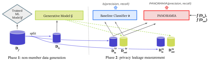
Figure 1: PANORAMIA’s two-phase privacy audit. Phase 1: training of generative model ${\mathcal{G}}$ using member data. Phase 2: training a MIA on a subset of member data and generated non-member data, along with the loss values of $f$ on these data points. The, the comparison of the performance of the MIA to a baseline classifier that does not have access to $f$ is performed. For notation please refer to Table 1.

2 Background

DP is the established privacy definition in the context of ML models as well as data analysis in general. We focus on the pure DP definition to quantify privacy with well-understood semantics. In a nutshell, DP is a property of a randomized mechanism (or computation) from datasets to an output space ${\mathcal{O}}$, noted $M:{\mathcal{D}}\rightarrow{\mathcal{O}}$. It is defined over neighboring datasets $D,D^{\prime}$, that differ by one element $x\in{\mathcal{X}}$ (we use the add/remove neighboring definition), which is $D^{\prime}=D\cup\{x\}$. Formally:

Definition 1 (Differential privacy Dwork et al. (2006)).

A randomized mechanism $M:{\mathcal{D}}\rightarrow{\mathcal{O}}$ is $\epsilon$-DP if for any two neighboring datasets $D$, $D^{\prime}\in{\mathcal{D}}$, and for any measurable output subset $O\subseteq{\mathcal{O}}$ it holds that:

$$P[M(D)\subseteq O]\leq e^{\varepsilon}P[M(D^{\prime})\subseteq O].$$

Since the neighboring definition is symmetric, so is the DP definition, and we also have that $P[M(D^{\prime})\subseteq O]\leq e^{\varepsilon}P[M(D)\subseteq O]$. Intuitively, $\epsilon$ upper-bounds the worst-case contribution of any individual example to the distribution over outputs of the computation (i.e., the model learned). More formally, $\epsilon$ is an upper-bound on the privacy loss incurred by observing an output $o$, defined as $\big{|}\ln\left(\frac{{\mathbb{P}}[M(D)=o]}{{\mathbb{P}}[M(D^{\prime})=o]}\right)\big{|}$, which quantifies how much an adversary can learn to distinguish $D$ and $D^{\prime}$ based on observing output $o$ from $M$. A smaller $\epsilon$ hence means higher privacy.

DP, MIA and privacy audits. To audit a DP training algorithm $M$ that outputs a model $f$, one can perform a MIA on datapoint $x$, trying to distinguish between a neighboring training sets $D$ and $D^{\prime}=D\cup\{x\}$. The MIA can be formalized as a hypothesis test to distinguish between ${\mathcal{H}}_{0}=D$ and ${\mathcal{H}}_{1}=D^{\prime}$ using the output of the computation $f$. Wasserman & Zhou (2010); Kairouz et al. (2015); Dong et al. (2019) show that any such test at significance level $\alpha$ (the False Positive Rate (FPR), or probability of rejecting ${\mathcal{H}}_{0}$ when it is true) has power (True Positive Rate (TPR), or the probability of rejecting ${\mathcal{H}}_{0}$ when ${\mathcal{H}}_{1}$ is indeed true) bounded by $e^{\epsilon}\alpha$. In practice, one repeats the process of training model $f$ with and without $x$ in the training set, and uses a MIA to guess whether $x$ was included. If the MIA has $\textrm{TPR}>e^{\epsilon}\textrm{FPR}$, the training procedure that outputs $f$ is not $\epsilon$-DP. This is the building block of most privacy audits Jagielski et al. (2020); Nasr et al. (2021); Zanella-Béguelin et al. (2022); Lu et al. (2023); Nasr et al. (2023).

Averaging over data instead of models with O(1). The above result bounds the success rate of MIAs when performed over several retrained models, on two alternative datasets $D$ and $D^{\prime}$. Steinke et al. (2023) show that it is possible to average over data when several data points independently differ between $D$ and $D^{\prime}$. Let $x_{1,m}$ be the number of data points independently included in the training set, and $s_{1,m}\in\{0,1\}^{m}$ be the vector encoding inclusion. $T_{0,m}\in{\mathbb{R}}^{m}$ represents any vector of guesses, with positive values for inclusion in the training set (member), negative values for non-member, and zero for abstaining. Then, if the training procedure is $\epsilon$-DP, Proposition 5.1 in Steinke et al. (2023) bounds the performance of guesses from $T$ with:

$${\mathbb{P}}\Big{[}\sum_{i=1}^{m} \max\{0,T_{i}\cdot S_{i}\}\geq v\ |\ T=t\Big{]}$$

$$\leq\underset{{S^{\prime}\sim\textrm{Bernoulli}(\frac{e^{\epsilon}}{1+e^{\epsilon}})^{m}}}{{\mathbb{P}}}\Big{[}\sum_{i=1}^{m}|t_{i}|\cdot S^{\prime}_{i}\geq v\Big{]}.$$

In other words, an audit (MIA) $T$ that can guess membership better than a Bernoulli random variable with probability $\frac{e^{\epsilon}}{1+e^{\epsilon}}$ refutes $\epsilon$-DP claim. In this work we build on this result, extending the algorithm (§3) and theoretical analysis (§4) to enable the use of generated data for non-members, which breaks the independence between data points.

3 PANORAMIA

Notation	Description
$f$	the target model to be audited.
${\mathcal{G}}$	the generative model
${\mathcal{D}}$	distribution over auditor samples
$D_{f}$	(subset of the) training set of the target model $f$ from ${\mathcal{D}}$
$D_{G}$	training set of the generative model ${\mathcal{G}}$, with $D_{G}\subset D_{f}$
$D_{\textrm{in}}$	member auditing set, with $D_{\textrm{in}}\subset D_{f}$ and $D_{\textrm{in}}\cap D_{G}=\{\}$
$D_{\textrm{out}}$	non-member auditing set, with $D_{\textrm{out}}\sim{\mathcal{G}}$
$D^{\{\textrm{tr},\textrm{te}\}}_{\{\textrm{in},\textrm{out}\}}$	training and testing splits of $D_{\textrm{in}}$ and $D_{\textrm{out}}$
$m$	$|D_{\textrm{in}}|=|D_{\textrm{out}}|\triangleq m$
$b$	baseline classifier for $D_{\textrm{in}}$ vs. $D_{\textrm{out}}$

Table 1: Summary of notations

Figure 1 summarizes the end-to-end PANORAMIA privacy audit while Table 1 summarizes the notations used in the rest of the paper. The privacy audit starts with a target model $f$, and a subset of its training data $D_{f}$ from distribution ${\mathcal{D}}$. For instance, ${\mathcal{D}}$ and $D_{f}$ could be the distribution and dataset of one participant in an FL training procedure which returns a final model $f$. The audit then proceeds in two phases.

Phase 1: In the first phase, PANORAMIA uses a subset of the known training data $D_{G}\subset D_{f}$ to train a generative model ${\mathcal{G}}$. The goal of the generative model ${\mathcal{G}}$ is to match the training data distribution ${\mathcal{D}}$ as closely as possible, which we formalize in Definition 3 (§4). At a high level, we require the generative model to put a high likelihood on data that is also likely under ${\mathcal{D}}$. This means that the generator needs to generate a large number of data points that are good (likely under ${\mathcal{D}}$), though it is allowed to occasionally generate bad samples (unlikely under ${\mathcal{D}}$). In §4, we demonstrate that this one-sided requirement is sufficient due to our focus on finding members (i.e., true positives) as opposed to also finding non-members (i.e., true negatives) in our audit game. PANORAMIA is agnostic to the generative modeling approach, as the only primitive we need is that of data synthesis, with potential approaches including GANs, VAEs or Diffusion Models. We can also fine-tune existing generators and filter generated samples as a post-processing phase. We leverage several such approaches in practice (§5, Appendix B). Using the generative model ${\mathcal{G}}$, we can synthesize non-member data, which corresponds to data that was not used in the training of target model $f$. Hence, we now have access to an independent dataset of member data $D_{\textrm{in}}=D_{f}\backslash D_{G}$, and a synthesized dataset of non-member data $D_{\textrm{out}}$ from ${\mathcal{G}}$, that we choose to be of the same size $m$ as $D_{\textrm{in}}$.

Phase 2: In the second phase, we leverage $D_{\textrm{in}}$ and $D_{\textrm{out}}$ to audit the privacy leakage of $f$ using a MIA. To this end, we split $D_{\textrm{in}},D_{\textrm{out}}$ into training and testing sets, respectively called $D^{\textrm{tr}}_{\textrm{in}},D^{\textrm{tr}}_{\textrm{out}}$ and $D^{\textrm{te}}_{\textrm{in}},D^{\textrm{te}}_{\textrm{out}}$. We use the training set to train a MIA (called PANORAMIA in Figure 1), a binary classifier that predicts whether a given datapoint is a member of $D_{f}$, the training set of the target model $f$. This MIA classifier makes its prediction based on both a training example $x$, as well as information from applying the target model $f$ to the input, such as the loss of the target model when applied to this example $\textrm{loss}(f(x))$, or the likelihood of the data $f(x)$ for language models (see §5, Appendix B for details). As discussed in §2, MIA performance is directly related to a lower-bound on possible $\epsilon$-DP values for the target model $f$. We use the test set to measure the MIA performance, using the precision at different recall values.

Previous results linking the performance of a MIA on several data-points to $\epsilon$-DP bounds rely on independence between members and non-members. This intuitively means that there is no information about membership in $x$. When the auditor controls the training process this independence is enforced by construction, by adding data points to the training set based on an independent coin flip. In PANORAMIA, we do not have independence between membership and $x$, as all non-members come from the generator ${\mathcal{G}}\neq{\mathcal{D}}$. Intuitively, this implies that there are two ways to guess membership and have high MIA precision: either using $f$ to detect membership (i.e., symptomatic of privacy leakage) or detecting generated data (i.e., not a symptom of privacy leakage). Since we are only interested in measuring privacy leakage, we cannot compare our MIA results to that of a random guess but have to account for the detection of generated data based on $x$ only. To do this, we compare the results of the MIA to that of a baseline classifier $b$ that guesses membership based exclusively on $x$, without access to $f$ or its predictions on $x$. The stronger this baseline, the better the removal of the effect of synthesized data detection. §5.1 details how to construct a strong baseline while Algorithm 1 summarizes the entire procedure. In the next section, we demonstrate how to relate the difference between the baseline $b$ and the MIA performance to the privacy loss $\epsilon$.

Algorithm 1 PANORAMIA

1:Input: Target ML model $f$, audit set size $m$, confidence $1-\beta$

2:Phase 1:

3:Split $D_{f}$ in $D_{G},D^{\textrm{tr}}_{\textrm{in}},D^{\textrm{te}}_{\textrm{in}}$, with $|D^{\textrm{te}}_{\textrm{in}}|=m$

4:Train generator ${\mathcal{G}}$ on $D_{G}$

5:Generate $D^{\textrm{tr}}_{\textrm{out}},D^{\textrm{te}}_{\textrm{out}}$ of size $|D^{\textrm{tr}}_{\textrm{in}}|,|D^{\textrm{te}}_{\textrm{in}}|$

6:Phase 2:

7:Train the baseline and MIA:

1:Label $D^{\textrm{tr}}_{\textrm{in}}$ as members, and $D^{\textrm{tr}}_{\textrm{out}}$ as non-members

2:Train $b$ to predict labels using $x\in D^{\textrm{tr}}_{\textrm{in}}\cup D^{\textrm{tr}}_{\textrm{out}}$

3:Train MIA to predict labels using $x\in D^{\textrm{tr}}_{\textrm{in}}\cup D^{\textrm{tr}}_{\textrm{out}}$ and $f(x)$

4:Measure privacy leakage (see §4):

1:Sample $s\sim\textrm{Bernoulli}(\frac{1}{2})^{m}$ $\triangleright$ Def.2

2:Create audit set $X=s\cdot D^{\textrm{te}}_{\textrm{in}}+(1-s)D^{\textrm{te}}_{\textrm{out}}$

3:Score each audit point for membership, creating $t^{b}\triangleq b(X)\in{\mathbb{R}}_{+}^{m}$ and $t^{a}\triangleq\textrm{MIA}(X)\in{\mathbb{R}}_{+}^{m}$

4:Set $v_{\textrm{ub}}^{b}(c,t)\triangleq\sup\ \{v:\beta^{b}(m,c,v,t)\leq\frac{\beta}{2}\}$ $\triangleright$ Prop.1

5:$c_{\textrm{lb}}=\max_{t,c}\mathds{1}\{t^{b}\geq t\}\cdot s\leq v_{\textrm{ub}}^{b}(c,\mathds{1}\{t^{b}\geq t\})$

6:Set $v_{\textrm{ub}}^{a}(c,\epsilon,t)\triangleq\sup\ \{v:\beta^{a}(m,c,\epsilon,v,t)\leq\frac{\beta}{2}\}$ $\triangleright$ Prop.2

7:$\{c\!+\!\epsilon\}_{\textrm{lb}}=\max_{t,c,\epsilon}\mathds{1}\{t^{a}\geq t\}\cdot s\leq v_{\textrm{ub}}^{a}(c,\epsilon,\mathds{1}\{t^{a}\geq t\})$

8:Return $\tilde{\epsilon}\triangleq\{c\!+\!\epsilon\}_{\textrm{lb}}-c_{\textrm{lb}}$

4 Quantifying Privacy Leakage with PANORAMIA

The first step to quantifying privacy leakage is to formalize an auditing game. PANORAMIA starts with $x^{\textrm{in}}\in{\mathcal{X}}^{m}$ training points from ${\mathcal{D}}$ (e.g., the data distribution of one participant in an FL setting), as well as $x^{\textrm{gen}}\in{\mathcal{X}}^{m}$ generated points from the generator distribution ${\mathcal{G}}$ ($x^{\textrm{gen}}\sim{\mathcal{G}}$). We construct a sequence auditing samples $x\in{\mathcal{X}}^{m}$ as follows:

Definition 2 (Auditing game).

$$s\sim\textrm{Bernoulli}(\frac{1}{2})^{m},\ \textrm{with}\ s_{i}\in\{0,1\},$$

$$x_{i}=(1-s_{i})x^{\textrm{gen}}_{i}+s_{i}x^{\textrm{in}}_{i},\ \forall i\in\{1,\ldots,m\}.$$

This means that $s$ is sampled independently to choose either the real ($s_{i}=1$) or generated ($s_{1}=0$) data point at each index $i$. This creates a sequence of $m$ examples that PANORAMIA will try to tell apart (i.e., guess $s$). The level of success achievable in this game quantifies the privacy leakage of the target model $f$. More precisely, we follow an analysis inspired by that of Steinke et al. (2023), but require several key technical changes to support auditing with no retraining using generated non-member data. To realize this, we first formalize PANORAMIA’s audit procedure as a hypothesis test on our auditing game, for which we construct a statistical test (§4.1). Then, we show how to use this hypothesis test to quantify privacy leakage as a lower confidence interval, and interpret the semantics of our privacy leakage measurement (§4.2).

4.1 Formalizing the Audit as a Hypothesis Test

We first need a notion of quality for our generator:

Definition 3 ($c$-closeness).

For all $c>0$, we say that a generative model ${\mathcal{G}}$ is $c$-close for data distribution ${\mathcal{D}}$ if:

$$\forall x\in{\mathcal{X}},\ e^{-c}{\mathbb{P}}_{\mathcal{D}}\big{[}x\big{]}\leq{\mathbb{P}}_{\mathcal{G}}\big{[}x\big{]}.$$

The smaller $c$, the better generator, a ${\mathcal{G}}$ assigns a probability to real data that cannot be much smaller than that of the real data distribution. We make two important remarks.
Remark 1: $c$-closeness is a strong requirement but it is achievable, at least for a large $c$. For instance, a uniform random generator is $c$-close to any distribution ${\mathcal{D}}$, with $c<\infty$. Of course $c$ would be very large, and the challenge in PANORAMIA is to create a generator that empirically has a small enough $c$.
Remark 2: Our definition of closeness is very similar to that of DP. This is not a coincidence as we will use this definition to be able to reject claims of both $c$-closeness for the generator and $\epsilon$-DP for the algorithm that gave the target model. We further note that, contrary to the DP definition, $c$-closeness is one-sided as we only bound ${\mathbb{P}}_{\mathcal{G}}$ from below. Intuitively, this means that the generator has to produce high-quality samples (i.e., samples likely under ${\mathcal{D}}$) with high enough probability but it does not require that all samples are good though. This one-sided measure of closeness is enabled by our focus on detecting members (i.e., true positives) as opposed to members and non-members, and puts less stringent requirements on the generator.

Using Definition 3, we can formulate the hypothesis test on the auditing game of Definition 2 that underpins our approach:

$${\mathcal{H}}:\textrm{generator}\ {\mathcal{G}}\ \textrm{is}\ c\textrm{-close, and target model}\ f\ \textrm{is}\ \epsilon\textrm{-DP}.$$

Note that, in a small abuse of language, we will often refer to $f$ as $\epsilon$-DP to say that $f$ is the output of an $\epsilon$-DP mechanism.

To construct a statistical test allowing us to reject ${\mathcal{H}}$ based on evidence, we define two key mechanisms (corresponding to PANORAMIA’s auditing scheme). First, the (potentially randomized) baseline guessing mechanism $B(s,x):\{0,1\}^{m}\times{\mathcal{X}}^{m}\rightarrow{\mathbb{R}}_{+}^{m}$, which outputs a (non-negative) score for the membership of each datapoint $x_{i}$, based on this datapoint only. That is, $B(s,x)=\{b(x_{1}),b(x_{2}),\ldots,b(x_{m})\}$.

Second, we define $A(s,x,f):\{0,1\}^{m}\times{\mathcal{X}}^{m}\times{\mathcal{F}}\rightarrow{\mathbb{R}}_{+}^{m}$, which outputs a (potentially randomized) non-negative score for the membership of each datapoint, with the guess for index $i$ depending on $x_{\leq i}$ and target model $f$. Note that if the target model $f$ is DP, then $A$ is DP w.r.t. inclusion in the auditing game $s$, outside of what is revealed by $x$. We are now ready to construct a hypothesis test for ${\mathcal{H}}$. First, we construct tests for each part of the hypothesis separately.

Proposition 1.

Let ${\mathcal{G}}$ be $c$-close, $S$ and $X$ be the random variables for $s$ and $x$ from Definition 2, and $T^{b}\triangleq B(S,X)$ be the vector of guesses from the baseline. Then, for all $v\in{\mathbb{R}}$ and all $t$ in the support of $T$:

$${\mathbb{P}}_{S,X,T^{b}}\Big{[}\sum_{i=1}^{m}T^{b}_{i}\cdot S_{i}\geq v\ |\ T^{b}=t^{b}\Big{]}$$

$$\leq\underset{{S^{\prime}\sim\textrm{Bernoulli}(\frac{e^{c}}{1+e^{c}})^{m}}}{{\mathbb{P}}}\Big{[}\sum_{i=1}^{m}t^{b}_{i}\cdot S^{\prime}_{i}\geq v\Big{]}\triangleq\beta^{b}(m,c,v,t^{b})$$

Proof.

Notice that under our baseline model $B(s,x)=\{b(x_{1}),b(x_{2}),\ldots,b(x_{m})\}$, and given that the $X_{i}$ are i.i.d., we have that: $S_{<i}\perp\!\!\!\!\perp T^{b}_{<i}\ |\ X_{<i}$, since $T^{b}_{i}=B(S,X)_{i}$’s distribution is entirely determined by $X_{i}$; and $S_{\leq i}\perp\!\!\!\!\perp T^{b}_{>i}\ |\ X_{<i}$ since the $X_{i}$ are sampled independently from the past.

We study the distribution of $S$ given a fixed prediction vector $t^{b}$, one element $i\in[m]$ at a time:

$${\mathbb{P}}\big{[}S_{i}=1\ |\ T^{b}=t^{b},S_{<i}=s_{<i},X_{\leq i}=x_{\leq i}\big{]}$$

$$={\mathbb{P}}\big{[}S_{i}=1\ |\ S_{<i}=s_{<i},X_{\leq i}=x_{\leq i}\big{]}$$

$$={\mathbb{P}}\big{[}X_{i}\ |\ S_{i}=1,S_{<i}=s_{<i},X_{<i}=x_{<i}\big{]}$$

$$\ \ \ \ \frac{{\mathbb{P}}\big{[}S_{i}=1\ |\ S_{<i}=s_{<i},X_{<i}=x_{<i}\big{]}}{{\mathbb{P}}\big{[}X_{i}\ |\ S_{<i}=s_{<i},X_{<i}=x_{<i}\big{]}}$$

$$=\frac{{\mathbb{P}}\big{[}X_{i}\ |\ S_{i}=1,S_{<i}=s_{<i},X_{<i}=x_{<i}\big{]}{\mathbb{P}}\big{[}S_{i}=1\big{]}}{{\mathbb{P}}\big{[}X_{i}\ |\ S_{<i}=s_{<i},X_{<i}=x_{<i}\big{]}}$$

$$=\frac{{\mathbb{P}}\big{[}X_{i}\ |\ S_{i}=1\big{]}\frac{1}{2}}{{\mathbb{P}}\big{[}X_{i}\ |\ S_{i}=1\big{]}\frac{1}{2}+{\mathbb{P}}\big{[}X_{i}\ |\ S_{i}=0\big{]}\frac{1}{2}}$$

$$=\frac{1}{1+\frac{{\mathbb{P}}\big{[}X_{i}\ |\ S_{i}=0\big{]}}{{\mathbb{P}}\big{[}X_{i}\ |\ S_{i}=1\big{]}}}=\frac{1}{1+\frac{{\mathbb{P}}_{\mathcal{G}}\big{[}X_{i}\big{]}}{{\mathbb{P}}_{\mathcal{D}}\big{[}X_{i}\big{]}}}\leq\frac{1}{1+e^{-c}}=\frac{e^{c}}{1+e^{c}}$$

The first equality uses the independence remarks at the beginning of the proof, the second relies on Bayes’ rule, while the third and fourth that $S_{i}$ is sampled i.i.d. from a Bernoulli with probability half, and $X_{i}$ i.i.d. conditioned on $S_{i}$. The last inequality uses Definition 3 for $c$-closeness.

Using this result and the law of total probability to introduce conditioning on $X_{\leq i}$, we get that:

$${\mathbb{P}}\big{[}S_{i}=1\ |\ T^{b}=t^{b},S_{<i}=s_{<i}\big{]}$$

$$=\sum_{x_{\leq i}}{\mathbb{P}}\big{[}S_{i}=1\ |\ T^{b}=t^{b},S_{<i}=s_{<i},X_{\leq i}=x_{\leq i}\big{]}$$

$$\ \ \ \ {\mathbb{P}}\big{[}X_{\leq i}=x_{\leq i}\ |\ T^{b}=t^{b},S_{<i}=s_{<i}\big{]}$$

$$\leq\sum_{x_{\leq i}}\frac{e^{c}}{1+e^{c}}{\mathbb{P}}\big{[}X_{\leq i}=x_{\leq i}\ |\ T^{b}=t^{b},S_{<i}=s_{<i}\big{]},$$

and hence that:

$${\mathbb{P}}\big{[}S_{i}=1\ |\ T^{b}=t^{b},S_{<i}=s_{<i}\big{]}\leq\frac{e^{c}}{1+e^{c}}$$ (1)

We can now proceed by induction: assume inductively that $W_{m-1}\triangleq\sum_{i=1}^{m-1}T^{b}_{i}\cdot S_{i}$ is stochastically dominated (see Definition 4.8 in Steinke et al. (2023)) by $W^{\prime}_{m-1}\triangleq\sum_{i=1}^{m-1}T^{b}_{i}\cdot S^{\prime}_{i}$, in which $S^{\prime}\sim\textrm{Bernoulli}(\frac{e^{c}}{1+e^{c}})^{m-1}$. Setting $W_{1}=W^{\prime}_{1}=0$ makes it true for $m=1$. Then, conditioned on $W_{m-1}$ and using Eq. 4, $T^{b}_{m}\cdot S_{m}=T_{m}\cdot\mathds{1}\{S_{m}=1\}$ is stochastically dominated by $T^{b}_{m}\cdot\textrm{Bernoulli}(\frac{e^{c}}{1+e^{c}})$. Applying Lemma 4.9 from Steinke et al. (2023) shows that $W_{m}$ is stochastically dominated by $W^{\prime}_{m}$, which proves the induction and implies the proposition’s statement. ∎

Proof.

In Appendix A.1. ∎

Now that we have a test to reject a claim that the generator ${\mathcal{G}}$ is $c$-close for the data distribution ${\mathcal{D}}$, we turn our attention to the second part of ${\mathcal{H}}$ which claims that the target model $f$ is the result of an $\epsilon$-DP mechanism.

Proposition 2.

Let ${\mathcal{G}}$ be $c$-close, $S$ and $X$ be the random variables for $s$ and $x$ from Definition 2, $f$ be $\epsilon$-DP, and $T^{a}\triangleq A(S,X,f)$ be the guesses from the membership audit. Then, for all $v\in{\mathbb{R}}$ and all $t$ in the support of $T$:

$${\mathbb{P}}_{S,X,T^{a}}\Big{[}\sum_{i=1}^{m}T^{a}_{i}\cdot S_{i}\geq v\ |\ T^{a}=t^{a}\Big{]}\leq$$

$$\underset{{S^{\prime}\sim\textrm{Bernoulli}(\frac{e^{c+\epsilon}}{1+e^{c+\epsilon}})^{m}}}{{\mathbb{P}}}\Big{[}\sum_{i=1}^{m}t^{a}_{i}\cdot S^{\prime}_{i}\geq v\Big{]}\triangleq\beta^{a}(m,c,\epsilon,v,t^{a})$$

Proof.

Fix some $t^{a}\in{\mathbb{R}}_{+}^{m}$. We study the distribution of $S$ one element $i\in[m]$ at a time:

$${\mathbb{P}}\big{[}S_{i}=1\ |\ T^{a}=t^{a},S_{<i}=s_{<i},X_{\leq i}=x_{\leq i}\big{]}$$

$$={\mathbb{P}}\big{[}T^{a}=t^{a}\ |\ S_{i}=1,S_{<i}=s_{<i},X_{\leq i}=x_{\leq i}\big{]}$$

$$\ \ \ \ \frac{{\mathbb{P}}\big{[}S_{i}=1\ |\ S_{<i}=s_{<i},X_{\leq i}=x_{\leq i}\big{]}}{{\mathbb{P}}\big{[}T^{a}=t^{a}\ |\ S_{<i}=s_{<i},X_{\leq i}=x_{\leq i}\big{]}}$$

$$\leq\frac{1}{1+e^{-\epsilon}\frac{{\mathbb{P}}\big{[}S_{i}=0\ |\ S_{<i}=s_{<i},X_{\leq i}=x_{\leq i}\big{]}}{{\mathbb{P}}\big{[}S_{i}=1\ |\ S_{<i}=s_{<i},X_{\leq i}=x_{\leq i}\big{]}}}$$

$$\leq\frac{1}{1+e^{-\epsilon}e^{-c}}=\frac{e^{c+\epsilon}}{1+e^{c+\epsilon}}$$

The first equality uses Bayes’ rule. The first inequality uses the decomposition:

$${\mathbb{P}}\big{[}T^{a}=t^{a}\ |\ S_{<i}=s_{<i},X_{\leq i}=x_{\leq i}\big{]}=$$

$$={\mathbb{P}}\big{[}T^{a}=t^{a}\ |\ S_{i}=1,S_{<i}=s_{<i},X_{\leq i}=x_{\leq i}\big{]}$$

$$\ \ \cdot{\mathbb{P}}\big{[}S_{i}=1\ |\ S_{<i}=s_{<i},X_{\leq i}=x_{\leq i}\big{]}$$

$$+{\mathbb{P}}\big{[}T^{a}=t^{a}\ |\ S_{i}=0,S_{<i}=s_{<i},X_{\leq i}=x_{\leq i}\big{]}$$

$$\ \ \cdot{\mathbb{P}}\big{[}S_{i}=0\ |\ S_{<i}=s_{<i},X_{\leq i}=x_{\leq i}\big{]},$$

and the fact that $A(s,x,f)$ is $\epsilon$-DP w.r.t. $s$ and hence that:

$$\frac{{\mathbb{P}}\big{[}T^{a}=t^{a}\ |\ S_{i}=0,S_{<i}=s_{<i},X_{\leq i}=x_{\leq i}\big{]}}{{\mathbb{P}}\big{[}T^{a}=t^{a}\ |\ S_{i}=1,S_{<i}=s_{<i},X_{\leq i}=x_{\leq i}\big{]}}\geq e^{-\epsilon}.$$

The second inequality uses that:

$$\frac{{\mathbb{P}}\big{[}S_{i}=0\ |\ S_{<i}=s_{<i},X_{\leq i}=x_{\leq i}\big{]}}{{\mathbb{P}}\big{[}S_{i}=1\ |\ S_{<i}=s_{<i},X_{\leq i}=x_{\leq i}\big{]}}$$

$$=\frac{{\mathbb{P}}\big{[}X_{i}=x_{i}\ |\ S_{i}=0,S_{<i}=s_{<i},X_{<i}=x_{<i}\big{]}}{{\mathbb{P}}\big{[}X_{i}=x_{i}\ |\ S_{i}=1,S_{<i}=s_{<i},X_{<i}=x_{<i}\big{]}}$$

$$\ \ \cdot\frac{{\mathbb{P}}\big{[}S_{i}=0\ |\ S_{<i}=s_{<i},X_{<i}=x_{<i}\big{]}}{{\mathbb{P}}\big{[}S_{i}=1\ |\ S_{<i}=s_{<i},X_{<i}=x_{<i}\big{]}}$$

$$=\frac{{\mathbb{P}}\big{[}X_{i}=x_{i}\ |\ S_{i}=0,S_{<i}=s_{<i},X_{<i}=x_{<i}\big{]}}{{\mathbb{P}}\big{[}X_{i}=x_{i}\ |\ S_{i}=1,S_{<i}=s_{<i},X_{<i}=x_{<i}\big{]}}\cdot\frac{1/2}{1/2}$$

$$=\frac{{\mathbb{P}}_{\mathcal{G}}\big{[}X_{i}\big{]}}{{\mathbb{P}}_{\mathcal{D}}\big{[}X_{i}\big{]}}\geq e^{-c}$$

As in Proposition 1, applying the law of total probability to introduce conditioning on $X_{\leq i}$ yields:

$${\mathbb{P}}\big{[}S_{i}=1\ |\ T^{a}=t^{a},S_{<i}=s_{<i}\big{]}\leq\frac{e^{c+\epsilon}}{1+e^{c+\epsilon}},$$ (2)

and we can proceed by induction. Assume inductively that $W_{m-1}\triangleq\sum_{i=1}^{m-1}T^{a}_{i}\cdot S_{i}$ is stochastically dominated (see Definition 4.8 in Steinke et al. (2023)) by $W^{\prime}_{m-1}\triangleq\sum_{i=1}^{m-1}T^{a}_{i}\cdot S^{\prime}_{i}$, in which $S^{\prime}\sim\textrm{Bernoulli}(\frac{e^{c+\epsilon}}{1+e^{c+\epsilon}})^{m-1}$. Setting $W_{1}=W^{\prime}_{1}=0$ makes it true for $m=1$. Then, conditioned on $W_{m-1}$ and using Equation 5, $T^{a}_{m}\cdot S_{m}=T^{a}_{m}\cdot\mathds{1}\{S_{m}=1\}$ is stochastically dominated by $T^{a}_{m}\cdot\textrm{Bernoulli}(\frac{e^{c+\epsilon}}{1+e^{c+\epsilon}})$. Applying Lemma 4.9 from Steinke et al. (2023) shows that $W_{m}$ is stochastically dominated by $W^{\prime}_{m}$, which proves the induction and implies the proposition’s statement. ∎

Proof.

In Appendix A.2. ∎

We can now provide a test for hypothesis ${\mathcal{H}}$, by applying a union bound over Propositions 1 and 2:

Corollary 1.

Let ${\mathcal{H}}$ be true, $T^{b}\triangleq B(S,X)$, and $T^{a}\triangleq A(S,X,f)$. Then:

$${\mathbb{P}}\Big{[}\sum_{i=1}^{m}T^{a}_{i}\cdot S_{i}\geq v^{a},\ \sum_{i=1}^{m}T^{b}_{i}\cdot S_{i}\geq v^{b}\ |\ T^{a}=t^{a},T^{b}=t^{b}\Big{]}$$

$$\leq\beta^{a}(m,c,\epsilon,v^{a},t^{a})+\beta^{b}(m,c,v^{b},t^{b})$$

To make things more concrete, let us instantiate Corollary 1 as we do in PANORAMIA. Our baseline ($B$ above) and MIA ($A$ above) classifiers return a membership guesses $T^{a,b}\in\{0,1\}^{m}$, with $1$ corresponding to membership. Let us call $r^{a,b}\triangleq\sum_{i}t_{i}^{a,b}$ the total number of predictions, and $\textrm{tp}^{a,b}\triangleq\sum_{i}t_{i}^{a,b}\cdot s_{i}$ the number of correct membership guesses (true positives). We also call the precision $\textrm{prec}^{a,b}\triangleq\frac{\textrm{tp}^{a,b}}{r^{a,b}}$. Using the following tail bound on the sum of Bernoulli random variables for simplicity and clarity (we use a tighter bound in practice, but this one is easier to read),

$$\underset{{S^{\prime}\sim\textrm{Bernoulli}(p)^{r}}}{{\mathbb{P}}}\Big{[}\sum_{i=1}^{r}\frac{S^{\prime}_{i}}{r}\geq p+\sqrt{\frac{\log(1/\beta)}{2r}}\Big{]}\leq\beta,$$

we can reject ${\mathcal{H}}$ at confidence level $\beta$ by setting $\beta^{a}=\beta^{b}=\frac{\beta}{2}$ and if either $\textrm{prec}^{b}\geq\frac{e^{c}}{1+e^{c}}+\sqrt{\frac{\log(2/\beta)}{2r^{b}}}$ or $\textrm{prec}^{a}\geq\frac{e^{c+\epsilon}}{1+e^{c+\epsilon}}+\sqrt{\frac{\log(2/\beta)}{2r^{a}}}$.

4.2 Quantifying Privacy Leakage and Interpretation

In an audit we would like to quantify $\epsilon$, not just reject a given $\epsilon$ claim. We use the hypothesis test from Corollary 1 to compute a confidence interval on $c$ and $\epsilon$. To do this, we first define an ordering between $(c,\epsilon)$ pairs, such that if $(c_{1},\epsilon_{1})\leq(c_{2},\epsilon_{2})$, the event (i.e., set of observations for $T^{a,b},S$) for which we can reject ${\mathcal{H}}(c_{2},\epsilon_{2})$ is included in the event for which we can reject ${\mathcal{H}}(c_{1},\epsilon_{1})$. That is, if we reject ${\mathcal{H}}$ for values $(c_{2},\epsilon_{2})$ based on audit observations, we also reject values $(c_{1},\epsilon_{1})$ based on the same observations.

We define the following lexicographic order to fit this assumption, based on the hypothesis test from Corollary 1:

$$(c_{1},\epsilon_{1})\leq(c_{2},\epsilon_{2})\ \textrm{if either}\ \begin{cases}c_{1}<c_{2},\ \textrm{or}\\ c_{1}=c_{2}\ \textrm{and}\ \epsilon_{1}\leq\epsilon_{2}\end{cases}$$ (3)

With this ordering, we have that:

Corollary 2.

For all $\beta\in]0,1]$, $m$, and observed $t^{a},t^{b}$, call $v_{\textrm{ub}}^{a}(c,\epsilon)\triangleq\sup\ \{v:\beta^{a}(m,c,\epsilon,v,t^{a})\leq\frac{\beta}{2}\}$ and $v_{\textrm{ub}}^{b}(c)\triangleq\sup\ \{v:\beta^{b}(m,c,v,t^{b})\leq\frac{\beta}{2}\}$. Then:

$${\mathbb{P}}\Big{[}(c,\epsilon)\geq\sup\big{\{}(c^{\prime},\epsilon^{\prime}):t^{a}\cdot s\leq v_{\textrm{ub}}^{a}(c^{\prime},\epsilon^{\prime})\ \textrm{and}\ t^{b}\cdot s\leq v_{\textrm{ub}}^{b}(c^{\prime})$$

$$\big{\}}\Big{]}\geq 1-\beta$$

Proof.

Apply Lemma 4.7 from Steinke et al. (2023) with the ordering from Eq. 3 and the test from Corollary 1. ∎

The lower confidence interval for $(c,\epsilon)$ at confidence $1-\beta$ is the largest $(c,\epsilon)$ pair that cannot be rejected using Corollary 1 with false rejection probability at most $\beta$. Hence, for a given confidence level $1-\beta$, PANORAMIA computes $(c_{\textrm{lb}},\tilde{\epsilon})$, the largest value for $(c,\epsilon)$ that it cannot reject. Note that Corollaries 1 and 2 rely on a union bound between two tests, one for $c$ and one for $c+\epsilon$. We can thus consider each test separately (at level $\beta/2$). In practice, we follow previous approaches Maddock et al. (2023); Steinke et al. (2023) and use the whole precision/recall curve. Each level of recall (i.e., threshold on $t^{a,b}$ to predict membership) corresponds to a bound on the precision, which we can compare to the empirical value. Separately for each test, we pick the level of recall yielding the highest lower-bound (Lines 4-7 in the last section of Algorithm 1). We next discuss the semantics of returned values, $(c_{\textrm{lb}},\tilde{\epsilon})$.

Audit semantics. Corollary 2 gives us a lower-bound for $(c,\epsilon)$, based on the ordering from Equation 3. To understand the value $\tilde{\epsilon}$ returned by PANORAMIA, we need to understand what the hypothesis test rejects. Rejecting ${\mathcal{H}}$ means either rejecting the claim about $c$, or the claim about $c+\epsilon$ (which is the reason for the ordering in Equation 3). With Corollary 2, we hence get both a lower-bound $c_{\textrm{lb}}$ on $c$, and $\{c\!+\!\epsilon\}_{\textrm{lb}}$ on $c+\epsilon$. Unfortunately, $\tilde{\epsilon}\triangleq\max\{0,\{c\!+\!\epsilon\}_{\textrm{lb}}-c_{\textrm{lb}}\}$, which is the value PANORAMIA returns, does not imply a lower-bound on $\epsilon$. Instead, we can claim that “PANORAMIA could not reject a claim of $c$-closeness for ${\mathcal{G}}$, and if this claim is tight, then $f$ cannot be the output of a mechanism that is $\tilde{\epsilon}$-DP”.

While this is not as strong a claim as typical lower-bounds on $\epsilon$-DP from prior privacy auditing works, we believe that this measure is useful in practice. Indeed, the $\tilde{\epsilon}$ measured by PANORAMIA is a quantitative privacy measurement, that is accurate (close to a lower-bound on $\epsilon$-DP) when the baseline performs well (and hence $c_{\textrm{lb}}$ is tight). Thus, when the baseline is good, $\tilde{\epsilon}$ can be interpreted as (close to) a lower bound on (pure) DP. In addition, since models on the same dataset and task share the same baseline, which does not depend on the audited model, PANORAMIA’s measurement can be used to directly compare privacy leakage between models. Thus, PANORAMIA opens a new capability, measuring privacy leakage of a trained model $f$ without access or control of the training pipeline, with an meaningfull and practically useful measurement, as we empirically show next.

5 Evaluation

ML Model	Dataset	Training Epoch	Test Accuracy	Model Variants Names*
ResNet101	CIFAR10	20, 50, 100	91.61%, 90.18%, 87.93%	ResNet101-E20, ResNet101-E50, ResNet101-E100,
Multi-Label CNN	CelebA	50, 100	81.77%, 78.12%	CNN_E50, CNN_E100
GPT-2	WikiText-2	12, 46, 92	Refer to Appendix B.2	GPT-2_E12, GPT-2_E46, GPT-2_E92
MLP Tabular Classification	Adult	10, 100	86%, 82%	MLP_E10, MLP_E100

Table 2: Train and Test Metrics for ML Models Audited. *”Model Variants” trained for different number of epochs $E$.

We instantiate PANORAMIA on target models for four tasks from three data modalities. For image classification, we consider the CIFAR10 Krizhevsky et al. (2009), and CelebA Liu et al. (2015) datasets, with varied target models: a four-layers CNN O’Shea & Nash (2015), a ResNet101 He et al. (2015) and a differentially-private ResNet18 He et al. (2015) trained with DP-SGD (Abadi et al., 2016) using Opacus (Yousefpour et al., 2021) at different values of $\epsilon$. We use StyleGAN2 Karras et al. (2020) for ${\mathcal{G}}$. For language models, we fine-tune small GPT-2 Radford et al. (2019) on the WikiText-2 train dataset Merity et al. (2016) (we also incorporate documents from WikiText-103 to obtain a larger dataset). ${\mathcal{G}}$ is again based on small GPT-2, and then fine-tuned on $D_{G}$. We generate samples using top-$p$ sampling Holtzman et al. (2019) and a held-out prompt dataset $D_{G}^{prompt}\subset D_{G}$. Finally, for classification on tabular data, we fit a Multi-Layer Perceptron (MLP) with 4 hidden layers trained on the Adult dataset Becker & Kohavi (1996), on a binary classification task predicting income $>\$50k$. We use the MST algorithm McKenna et al. (2021) for ${\mathcal{G}}$.

Table 2 summarizes the tasks, models and performance, as well as the respective names we use to show results. Due to lack of space, more details on the settings, the models used and implementation details are provided in  Appendix B. Our results are organized as follows. First, we evaluate the strength of our baseline (§5.1), on which the semantics of PANORAMIA’s audit rely. Second, we show what PANORAMIA detects meaningful privacy leakage in our settings, comparable to the lower-bounds provided by the O(1) approach (Steinke et al., 2023) (though under weaker requirements) (§5.2). Finally, we show that PANORAMIA can detect varying amounts of leakage from models with controlled data leakage using model size and DP (§5.3).

5.1 Baseline Design and Evaluation

Our MIA is a loss-based attack based on an attack model that takes as input a datapoint $x$ as well as the value of the loss of target model $f$ on point $x$. Appendix B details the architectures used for the attack model for each data modality. Recall from §4.2 the importance of having a tight $c_{\textrm{lb}}$ for our measure $\tilde{\epsilon}$ to be close to a lower-bound on $\epsilon$-DP, which also requires a strong baseline. To increase the performance of our baseline $b$, we mimic the role of the target model $f$’s loss in the MIA using a helper model $h$, which adds a loss-based feature to $b$.

This new feature can be viewed as side information about the data distribution. Table 3 shows the $c_{\textrm{lb}}$ value under different designs for $h$. The best performance is consistently when $h$ is trained on synthetic data before being used as a feature to train the $b$. Indeed, such a design reaches a $c_{\textrm{lb}}$ up to $1.36$ larger that without any helper (CIFAR10) and $0.16$ higher than when training on real non-member data without requiring access to real non-member data, a key requirement in PANORAMIA. We adopt this design in all the following experiments. In Figure 2 we show that the baseline has enough training data (vertical dashed line) to reach its best performance. Section C.1, shows similar results on all modalities (except on tabular data, in which more data for $b$ would help a bit), as well as different architectures that we tried. All these evidences confirm the strength of our baseline.

Baseline model $c_{lb}$ CIFAR-10 Baseline_{$D_{h}^{\text{tr}}=\text{gen}$} 2.508 CIFAR-10 Baseline_{$D_{h}^{\text{tr}}=\text{real}$} 2.37 CIFAR-10 Baseline_{no helper} 1.15 CelebA Baseline_{$D_{h}^{\text{tr}}=\text{gen}$} 2.03 CelebA Baseline_{$D_{h}^{\text{tr}}=\text{real}$} 1.67 CelebA Baseline_{no helper} 0.91 WikiText-2 Baseline_{$D_{h}^{\text{tr}}=\text{gen}$} 2.61 WikiText-2 Baseline_{$D_{h}^{\text{tr}}=\text{real}$} 2.59 WikiText-2 Baseline_{no helper} 2.34 Adult Baseline_{$D_{h}^{\text{tr}}=\text{gen}$} 2.34 Adult Baseline_{$D_{h}^{\text{tr}}=\text{real}$} 2.18 Adult Baseline_{no helper} 2.01

Table 3: Baseline evaluation with different helper model scenarios

Figure 2: CIFAR-10 baseline on increasing training size.

5.2 Main Auditing Results

We run PANORAMIA on models with different values of over-fitting (by varying the number of epochs, see the final accuracy on Table 2) for each data modality. More over-fitted models are known to leak more information about their training data due to memorization Yeom et al. (2018); Carlini et al. (2019; 2022a). To show the auditing power of PANORAMIA, we compare it with two strong approaches to lower-bounding privacy loss. First, we use a variation of our approach using real non-member data instead of generated data (called RM;RN for Real Members; Real Non-members). While this basically removes the role of the baseline ($c_{\textrm{lb}}=0$), it requires access to a large sample of non-member data from the same distributions as members (hard requirement) or the possibility of training costly shadow models to create such non-members. Second, we rely on the O(1) audit from Steinke et al. (2023), which is similar to the previous approach but predicts membership based on a loss threshold while also leveraging guesses on non-members in its statistical test. Note that this technique requires control of the training process. The privacy loss measured by these techniques gives a target what we hope PANORAMIA to detect.

Target model $f$	Audit	$\mathbf{c_{\textrm{lb}}}$	$\mathbf{\{\epsilon+c\}_{\textrm{lb}}}$	$\mathbf{\tilde{\epsilon}}$	$\mathbf{\epsilon}$
	PANORAMIA	$2.508$	$2.83$	$0.32$	-
ResNet101_E20	PANORAMIARM;RN	$0$	$0.42$	-	$0.42$
	O (1) RM;RN	-	-	-	$0.52$
	PANORAMIA	$2.508$	$3.15$	$0.64$	-
ResNet101_E50	PANORAMIARM;RN	$0$	$0.61$	-	$0.61$
	O (1) RM;RN	-	-	-	$0.81$
	PANORAMIA	$2.508$	$3.47$	$0.962$	-
ResNet101_E100	PANORAMIARM;RN	$0$	$1.03$	-	$1.03$
	O (1) RM;RN	-	-	-	$1.40$
	PANORAMIA	$2.01$	$2.50$	$0.49$	-
CNN_E50	PANORAMIARM;RN	$0$		-	0.76
	O (1) RM;RN	-	-	-	0.99
	PANORAMIA	$2.01$	$3.03$	$1.02$	-
CNN_E100	PANORAMIARM;RN	$0$		-	1.26
	O (1) RM;RN	-	-	-	1.53
	PANORAMIA	$3.78$	$3.47$	$0$	-
GPT2_E12	PANORAMIARM;RN	$0$	$0.30$	-	$0.30$
	O (1) RM;RN	-	-	-	$1.54$
	PANORAMIA	$3.78$	$4.07$	$0.29$	-
GPT2_E46	PANORAMIARM;RN	$0$	$2.37$	-	$2.37$
	O (1) RM;RN	-	-	-	$4.12$
	PANORAMIA	$3.78$	$5.06$	$1.28$	-
GPT2_E92	PANORAMIARM;RN	$0$	$3.45$	-	$3.45$
	O (1) RM;RN	-	-	-	$5.43$
	PANORAMIA	$2.37$	$2.47$	$0.10$	-
MLP_E10	O (1) RM;RN	-	-	-	$0.$
	PANORAMIA	$2.37$	$2.71$	$0.34$	-
MLP_E100	O (1) RM;RN	-	-	-	$0.23$
	PANORAMIA	$1.25$	$1.62$	$0.37$	-
MLP_E100_half	PANORAMIARM;RN	$0$	$0.64$	-	$0.64$
	O (1) RM;RN	-	-	-	$0.22$

Table 4: Privacy audits on different target models.

LABEL:fig:eval:comparison_precision shows the precision of $b$ and PANORAMIA at different levels of recall, and LABEL:fig:eval:comparison the corresponding value of $\{c+\epsilon\}_{lb}$ (or $c_{\textrm{lb}}$ for $b$). Dashed lines show the maximum value of $\{c+\epsilon\}_{lb}$/$c_{\textrm{lb}}$ achieved (Fig. LABEL:fig:eval:comparison) (returned by PANORAMIA), and the precision implying these values at different recalls (Fig. LABEL:fig:eval:comparison_precision). Table 4 summarizes those $\{c+\epsilon\}_{lb}$/$c_{\textrm{lb}}$ values, as well as the $\epsilon$ measured by existing approaches. We make two key observations.

First, the best prior method (whether RM;RN or O(1)) measures a larger privacy loss ($\tilde{\epsilon}\leq\epsilon$), except on tabular data. Those surprising results are likely due to PANORAMIA’s use of both raw data and the target model’s loss in an ML MIA model, whereas O(1) uses a threshold value on the loss only. Overall, these results empirically confirm the strength of $b$, as we do not seem to spuriously assign differences between ${\mathcal{G}}$ and ${\mathcal{D}}$ to our privacy loss proxy $\tilde{\epsilon}$. We also note that O(1) tends to perform better, due to its ability to rely on non-member detection, which improves the power of the statistical test at equal data sizes. Such tests are not available in PANORAMIA given our one-sided closeness definition for ${\mathcal{G}}$ (see §4), and we keep that same one-sided design for RM;RN for comparison’s sake.

Second, the values of $\tilde{\epsilon}$ measured by PANORAMIA are close to those of the methods against which we compared. In particular, despite a more restrictive adversary model (i.e., no non-member data, no control over the training process, and no shadow model training), PANORAMIA is able to detect meaningful amounts of privacy loss, comparable to that of state-of-the-art methods! For instance, on a non-overfitted CIFAR-10 model (E20), PANORAMIA detects a privacy loss of $0.32$, while using real non-member (RM;RN) data yields $0.42$, and controlling the training process $O(1)$ gets $0.52$. The relative gap gets even closer on models that reveal more about their training data. Indeed, for the most over-fitted model (E100), $\tilde{\epsilon}=0.96$ is very close to RM;RN ($\epsilon=1.0$) and O(1) ($\epsilon=1.4$). This also confirms that the leakage detected by PANORAMIA on increasingly over-fitted models does augment, which is confirmed by prior state-of-the-art methods. For instance, NLP models’ $\tilde{\epsilon}$ goes from $0.18$ to $1.28$ ($1.54$ to $5.43$ for O(1)), and tabular data MLPs from $0.1$ to $0.34$ ($0$ to $0.23$ for O(1)).

5.3 Detecting Controlled Variations in Privacy Loss

Models of varying complexity: Carlini et al. (2021) have shown that larger models tend to have bigger privacy losses. To confirm this, we conducted an audit of ML models with varying numbers of parameters, from a $\approx 4M$ parameters Wide ResNet-28-2, to a $25.5M$ parameters ResNet-50, and a $44.5M$ parameters ResNet-101. LABEL:subfig:var_complexities shows that PANORAMIA does detect increasing privacy leakage, with $\tilde{\epsilon}_{wide-resnet}\leq\tilde{\epsilon}_{resnet50}\leq\tilde{\epsilon}_{resnet101}$.

Target model	Audit	$\mathbf{c_{lb}}$	$\mathbf{\varepsilon+c_{lb}}$	$\mathbf{\tilde{\varepsilon}}$	$\mathbf{\varepsilon}$
ResNet18 $\epsilon=\infty$	PANORAMIA RM;GN	2.508	3.6698	1.161	-
	O (1) RM;RN	-	-	-	1.565
ResNet18 $\epsilon=15$	PANORAMIA RM;GN	2.508	3.5707	1.062	-
	O (1) RM;RN	-	-	-	1.22
ResNet18 $\epsilon=10$	PANORAMIA RM;GN	2.508	2.8	0.3	-
	O (1) RM;RN	-	-	-	0.14
ResNet18 $\epsilon=2$	PANORAMIA RM;GN	2.508	2.065	0	-
	O (1) RM;RN	-	-	-	0.08
ResNet18 $\epsilon=1$	PANORAMIA RM;GN	2.508	1.982	0	-
	O (1) RM;RN	-	-	-	0

Table 5: $\epsilon$-DP ResNet18 on CIFAR-10.

DP models: Another avenue to varying privacy leakage is by training DP models with diverse values of $\epsilon$. We evaluate PANORAMIA on DP ResNet-18 models on CIFAR10, with $\epsilon$ values shown on Table 5 and LABEL:subfig:resnet18-dp-fig. The hyper-parameters were tuned independently for the highest train accuracy (see Appendix C.6 for more results and discussion). As the results show, neither PANORAMIA or O(1) detect privacy loss on the most private models ($\epsilon=1,2$). At higher values of $\epsilon=10,15$ (i.e., less private models) and $\epsilon=\infty$ (i.e., non-private model) PANORAMIA does detect an increasing level of privacy leakage with $\tilde{\epsilon}_{\epsilon=10}<\tilde{\epsilon}_{\epsilon=15}<\tilde{\epsilon}_{\epsilon=\infty}$. In this regime, the O(1) approach detects a larger (except for $\epsilon=10$, in which PANORAMIA surprisingly detects a slightly larger value), though comparable, amount of privacy loss.

Appendix A Proofs

For both Proposition 1 and Proposition 2, we state the proposition again for convenience before proving it.

A.1 Proof of Proposition 1

Proposition 1.

Let ${\mathcal{G}}$ be $c$-close, and $T^{b}\triangleq B(S,X)$ be the guess from the baseline. Then, for all $v\in{\mathbb{R}}$ and all $t$ in the support of $T$:

$${\mathbb{P}}_{S,X,T^{b}}\Big{[}\sum_{i=1}^{m}T^{b}_{i}\cdot S_{i}\geq v\ |\ T^{b}=t^{b}\Big{]}$$

$$\leq\underset{{S^{\prime}\sim\textrm{Bernoulli}(\frac{e^{c}}{1+e^{c}})^{m}}}{{\mathbb{P}}}\Big{[}\sum_{i=1}^{m}t^{b}_{i}\cdot S^{\prime}_{i}\geq v\Big{]}\triangleq\beta^{b}(m,c,v,t^{b})$$

Proof.

Notice that under our baseline model $B(s,x)=\{b(x_{1}),b(x_{2}),\ldots,b(x_{m})\}$, and given that the $X_{i}$ are i.i.d., we have that: $S_{<i}\perp\!\!\!\!\perp T^{b}_{<i}\ |\ X_{<i}$, since $T^{b}_{i}=B(S,X)_{i}$’s distribution is entirely determined by $X_{i}$; and $S_{\leq i}\perp\!\!\!\!\perp T^{b}_{>i}\ |\ X_{<i}$ since the $X_{i}$ are sampled independently from the past.

We study the distribution of $S$ given a fixed prediction vector $t^{b}$, one element $i\in[m]$ at a time:

$${\mathbb{P}}\big{[}S_{i}=1\ |\ T^{b}=t^{b},S_{<i}=s_{<i},X_{\leq i}=x_{\leq i}\big{]}$$

$$={\mathbb{P}}\big{[}S_{i}=1\ |\ S_{<i}=s_{<i},X_{\leq i}=x_{\leq i}\big{]}$$

$$={\mathbb{P}}\big{[}X_{i}\ |\ S_{i}=1,S_{<i}=s_{<i},X_{<i}=x_{<i}\big{]}$$

$$\ \ \ \ \frac{{\mathbb{P}}\big{[}S_{i}=1\ |\ S_{<i}=s_{<i},X_{<i}=x_{<i}\big{]}}{{\mathbb{P}}\big{[}X_{i}\ |\ S_{<i}=s_{<i},X_{<i}=x_{<i}\big{]}}$$

$$=\frac{{\mathbb{P}}\big{[}X_{i}\ |\ S_{i}=1,S_{<i}=s_{<i},X_{<i}=x_{<i}\big{]}{\mathbb{P}}\big{[}S_{i}=1\big{]}}{{\mathbb{P}}\big{[}X_{i}\ |\ S_{<i}=s_{<i},X_{<i}=x_{<i}\big{]}}$$

$$=\frac{{\mathbb{P}}\big{[}X_{i}\ |\ S_{i}=1\big{]}\frac{1}{2}}{{\mathbb{P}}\big{[}X_{i}\ |\ S_{i}=1\big{]}\frac{1}{2}+{\mathbb{P}}\big{[}X_{i}\ |\ S_{i}=0\big{]}\frac{1}{2}}$$

$$=\frac{1}{1+\frac{{\mathbb{P}}\big{[}X_{i}\ |\ S_{i}=0\big{]}}{{\mathbb{P}}\big{[}X_{i}\ |\ S_{i}=1\big{]}}}=\frac{1}{1+\frac{{\mathbb{P}}_{\mathcal{G}}\big{[}X_{i}\big{]}}{{\mathbb{P}}_{\mathcal{D}}\big{[}X_{i}\big{]}}}\leq\frac{1}{1+e^{-c}}=\frac{e^{c}}{1+e^{c}}$$

The first equality uses the independence remarks at the beginning of the proof, the second relies Bayes’ rule, while the third and fourth that $S_{i}$ is sampled i.i.d from a Bernoulli with probability half, and $X_{i}$ i.i.d. conditioned on $S_{i}$. The last inequality uses Definition 3 for $c$-closeness.

Using this result and the law of total probability to introduce conditioning on $X_{\leq i}$, we get that:

$${\mathbb{P}}\big{[}S_{i}=1\ |\ T^{b}=t^{b},S_{<i}=s_{<i}\big{]}$$

$$=\sum_{x_{\leq i}}{\mathbb{P}}\big{[}S_{i}=1\ |\ T^{b}=t^{b},S_{<i}=s_{<i},X_{\leq i}=x_{\leq i}\big{]}$$

$$\ \ \ \ {\mathbb{P}}\big{[}X_{\leq i}=x_{\leq i}\ |\ T^{b}=t^{b},S_{<i}=s_{<i}\big{]}$$

$$\leq\sum_{x_{\leq i}}\frac{e^{c}}{1+e^{c}}{\mathbb{P}}\big{[}X_{\leq i}=x_{\leq i}\ |\ T^{b}=t^{b},S_{<i}=s_{<i}\big{]},$$

and hence that:

$${\mathbb{P}}\big{[}S_{i}=1\ |\ T^{b}=t^{b},S_{<i}=s_{<i}\big{]}\leq\frac{e^{c}}{1+e^{c}}$$ (4)

We can now proceed by induction: assume inductively that $W_{m-1}\triangleq\sum_{i=1}^{m-1}T^{b}_{i}\cdot S_{i}$ is stochastically dominated (see Definition 4.8 in Steinke et al. (2023)) by $W^{\prime}_{m-1}\triangleq\sum_{i=1}^{m-1}T^{b}_{i}\cdot S^{\prime}_{i}$, in which $S^{\prime}\sim\textrm{Bernoulli}(\frac{e^{c}}{1+e^{c}})^{m-1}$. Setting $W_{1}=W^{\prime}_{1}=0$ makes it true for $m=1$. Then, conditioned on $W_{m-1}$ and using Eq. 4, $T^{b}_{m}\cdot S_{m}=T_{m}\cdot\mathds{1}\{S_{m}=1\}$ is stochastically dominated by $T^{b}_{m}\cdot\textrm{Bernoulli}(\frac{e^{c}}{1+e^{c}})$. Applying Lemma 4.9 from Steinke et al. (2023) shows that $W_{m}$ is stochastically dominated by $W^{\prime}_{m}$, which proves the induction and implies the proposition’s statement. ∎

A.2 Proof of Proposition 2

Proposition 2.

Let ${\mathcal{G}}$ be $c$-close, $f$ be $\epsilon$-DP, and $T^{a}\triangleq A(S,X,f)$ be the guess from the membership audit. Then, for all $v\in{\mathbb{R}}$ and all $t$ in the support of $T$:

$${\mathbb{P}}_{S,X,T^{a}}\Big{[}\sum_{i=1}^{m}T^{a}_{i}\cdot S_{i}\geq v\ |\ T^{a}=t^{a}\Big{]}$$

$$\leq\underset{{S^{\prime}\sim\textrm{Bernoulli}(\frac{e^{c+\epsilon}}{1+e^{c+\epsilon}})^{m}}}{{\mathbb{P}}}\Big{[}\sum_{i=1}^{m}t^{a}_{i}\cdot S^{\prime}_{i}\geq v\Big{]}\triangleq\beta^{a}(m,c,\epsilon,v,t^{a})$$

Proof.

Fix some $t^{a}\in{\mathbb{R}}_{+}^{m}$. We study the distribution of $S$ one element $i\in[m]$ at a time:

$${\mathbb{P}}\big{[}S_{i}=1\ |\ T^{a}=t^{a},S_{<i}=s_{<i},X_{\leq i}=x_{\leq i}\big{]}$$

$$={\mathbb{P}}\big{[}T^{a}=t^{a}\ |\ S_{i}=1,S_{<i}=s_{<i},X_{\leq i}=x_{\leq i}\big{]}$$

$$\ \ \ \ \frac{{\mathbb{P}}\big{[}S_{i}=1\ |\ S_{<i}=s_{<i},X_{\leq i}=x_{\leq i}\big{]}}{{\mathbb{P}}\big{[}T^{a}=t^{a}\ |\ S_{<i}=s_{<i},X_{\leq i}=x_{\leq i}\big{]}}$$

$$\leq\frac{1}{1+e^{-\epsilon}\frac{{\mathbb{P}}\big{[}S_{i}=0\ |\ S_{<i}=s_{<i},X_{\leq i}=x_{\leq i}\big{]}}{{\mathbb{P}}\big{[}S_{i}=1\ |\ S_{<i}=s_{<i},X_{\leq i}=x_{\leq i}\big{]}}}$$

$$\leq\frac{1}{1+e^{-\epsilon}e^{-c}}=\frac{e^{c+\epsilon}}{1+e^{c+\epsilon}}$$

The first equality uses Bayes’ rule. The first inequality uses the decomposition:

$${\mathbb{P}}\big{[}T^{a}=t^{a}\ |\ S_{<i}=s_{<i},X_{\leq i}=x_{\leq i}\big{]}=$$

$$={\mathbb{P}}\big{[}T^{a}=t^{a}\ |\ S_{i}=1,S_{<i}=s_{<i},X_{\leq i}=x_{\leq i}\big{]}$$

$$\ \ \cdot{\mathbb{P}}\big{[}S_{i}=1\ |\ S_{<i}=s_{<i},X_{\leq i}=x_{\leq i}\big{]}$$

$$+{\mathbb{P}}\big{[}T^{a}=t^{a}\ |\ S_{i}=0,S_{<i}=s_{<i},X_{\leq i}=x_{\leq i}\big{]}$$

$$\ \ \cdot{\mathbb{P}}\big{[}S_{i}=0\ |\ S_{<i}=s_{<i},X_{\leq i}=x_{\leq i}\big{]},$$

and the fact that $A(s,x,f)$ is $\epsilon$-DP w.r.t. $s$ and hence that:

$$\frac{{\mathbb{P}}\big{[}T^{a}=t^{a}\ |\ S_{i}=0,S_{<i}=s_{<i},X_{\leq i}=x_{\leq i}\big{]}}{{\mathbb{P}}\big{[}T^{a}=t^{a}\ |\ S_{i}=1,S_{<i}=s_{<i},X_{\leq i}=x_{\leq i}\big{]}}\geq e^{-\epsilon}.$$

The second inequality uses that:

$$\frac{{\mathbb{P}}\big{[}S_{i}=0\ |\ S_{<i}=s_{<i},X_{\leq i}=x_{\leq i}\big{]}}{{\mathbb{P}}\big{[}S_{i}=1\ |\ S_{<i}=s_{<i},X_{\leq i}=x_{\leq i}\big{]}}$$

$$=\frac{{\mathbb{P}}\big{[}X_{i}=x_{i}\ |\ S_{i}=0,S_{<i}=s_{<i},X_{<i}=x_{<i}\big{]}}{{\mathbb{P}}\big{[}X_{i}=x_{i}\ |\ S_{i}=1,S_{<i}=s_{<i},X_{<i}=x_{<i}\big{]}}$$

$$\ \ \cdot\frac{{\mathbb{P}}\big{[}S_{i}=0\ |\ S_{<i}=s_{<i},X_{<i}=x_{<i}\big{]}}{{\mathbb{P}}\big{[}S_{i}=1\ |\ S_{<i}=s_{<i},X_{<i}=x_{<i}\big{]}}$$

$$=\frac{{\mathbb{P}}\big{[}X_{i}=x_{i}\ |\ S_{i}=0,S_{<i}=s_{<i},X_{<i}=x_{<i}\big{]}}{{\mathbb{P}}\big{[}X_{i}=x_{i}\ |\ S_{i}=1,S_{<i}=s_{<i},X_{<i}=x_{<i}\big{]}}\cdot\frac{1/2}{1/2}$$

$$=\frac{{\mathbb{P}}_{\mathcal{G}}\big{[}X_{i}\big{]}}{{\mathbb{P}}_{\mathcal{D}}\big{[}X_{i}\big{]}}\geq e^{-c}$$

As in Proposition 1, applying the law of total probability to introduce conditioning on $X_{\leq i}$ yields:

$${\mathbb{P}}\big{[}S_{i}=1\ |\ T^{a}=t^{a},S_{<i}=s_{<i}\big{]}\leq\frac{e^{c+\epsilon}}{1+e^{c+\epsilon}},$$ (5)

and we can proceed by induction. Assume inductively that $W_{m-1}\triangleq\sum_{i=1}^{m-1}T^{a}_{i}\cdot S_{i}$ is stochastically dominated (see Definition 4.8 in Steinke et al. (2023)) by $W^{\prime}_{m-1}\triangleq\sum_{i=1}^{m-1}T^{a}_{i}\cdot S^{\prime}_{i}$, in which $S^{\prime}\sim\textrm{Bernoulli}(\frac{e^{c+\epsilon}}{1+e^{c+\epsilon}})^{m-1}$. Setting $W_{1}=W^{\prime}_{1}=0$ makes it true for $m=1$. Then, conditioned on $W_{m-1}$ and using Eq. 5, $T^{a}_{m}\cdot S_{m}=T^{a}_{m}\cdot\mathds{1}\{S_{m}=1\}$ is stochastically dominated by $T^{a}_{m}\cdot\textrm{Bernoulli}(\frac{e^{c+\epsilon}}{1+e^{c+\epsilon}})$. Applying Lemma 4.9 from Steinke et al. (2023) shows that $W_{m}$ is stochastically dominated by $W^{\prime}_{m}$, which proves the induction and implies the proposition’s statement. ∎

Appendix B Experimental Details

Hereafter, we provide the details about the datasets and models trained in our experiments.

B.1 Image data

Target models. We audit target models with the following architectures: a Multi-Label Convolutional Neural Network (CNN) with four layers O’Shea & Nash (2015), and the ResNet101 He et al. (2015). We also include in our analysis, differentially-private models for ResNet18 He et al. (2015) and WideResNet-16-4 Zagoruyko & Komodakis (2017) models as targets, with $\epsilon=1,2,4,6,10,15,20$. The ResNet-based models are trained on CIFAR10 using $50k$ images Krizhevsky et al. (2009) of $32$x$32$ resolution. For all CIFAR10 based classification models (apart from the DP ones), we use a training batch size of 64. The associated test accuracies and epochs are mentioned in Table 2. The Multi-Label CNN is trained on $200k$ images of CelebA Liu et al. (2015) of $128$x$128$ resolution, training batch-size 32, to predict $40$ attributes associated with each image.

Generator. For both image datasets, we use StyleGAN2 Karras et al. (2020) to train the generative model ${\mathcal{G}}$ from scratch on $D_{G}$, and produce non-member images. For CIFAR10 dataset, we use a $10,000$ out of $50,000$ images from the training data of the target model to train the generative model. For the CelebA dataset, we select $35,000$ out of $200,000$ images from the training data of the target model to train the generative model. Generated images will in turn serve as non-members for performing the MIAs. Figure LABEL:datasets shows examples of member and non-member images used in our experiments. In the case of CelebA, we also introduce a vanilla CNN as a classifier or filter to distinguish between fake and real images, and remove any poor-quality images that the classifier detects with high confidence. The data used to train this classifier was the same data used to train StyleGAN2, which ensures that the generated high-resolution images are of high quality.

MIA and Baseline training. For the MIA, we follow a loss-based attack approach: PANORAMIA takes as input raw member and non-member data points for training along with the loss values the target model $f$ attributes to these data points. More precisely, the training set of PANORAMIA is:

$$(D^{tr}_{in},f(D^{tr}_{in}))\cup(D^{tr}_{out},f(D^{tr}_{out}))$$

In §4.2, we discussed the importance of having a tight $c_{\textrm{lb}}$ so that our measure, $\tilde{\epsilon}$, becomes close to a lower-bound on $\epsilon$-DP, which requires a strong baseline. To strengthen our baseline, we introduce the helper model $h$, which helps the baseline model $b$ by supplying additional features (i.e., embeddings) that can be viewed as side information about the data distribution. The motivation is that $h$’s features might differ between samples from ${\mathcal{D}}$ and ${\mathcal{D}}^{\prime}$, enhancing the performance of the baseline classifier. This embedding model $h$ is similar in design to $f$ (same task and architecture) but is trained on synthetic data that is close in distribution to the real member data distribution. Whether for the baseline or MIA, we use side information models ($h$ and $f$, respectively) by concatenating the loss of $h(x)$ and $f(x)$ to the final feature representation (more details are provided later) before a last layer of the MIA/Baseline makes the membership the prediction. Since we need labels to compute the loss, we label synthetic images with a Wide ResNet-28-2 in the case of CIFAR10, and a Multi-Label CNN of similar architecture as the target model in the case of CelebA labeling. For both instances, we used a subset of the data, that was used to train the respective generative models, to train the “labeler” classifiers as well.

We use two different modules for each MIA and Baseline training. More precisely, the first module optimizes image classification using a built-in Pytorch ResNet101 classifier. The second module, in the form of a multi-layer perceptron, focuses on classifying member and non-member labels via loss values attributed to these data points by $f$ as input for the loss module of MIA and losses of $e$ to the baseline $b$ respectively. We then stack the scores of both image and loss modules into a logistic regression task (as a form of meta-learning) to get the final outputs for member and non-member data points by MIA and baseline $b$. The MIA and baseline are trained on $4500$ data samples (half members and half generated non-members). The test dataset consists of $10000$ samples, again half members and half generated non-members. The actual and final number of members and non-members that ended up in the test set depends on the Bernoulli samples in our auditing game.

B.2 Language Modeling

Target model. The target model (a small GPT-2 Radford et al. (2019)) task is causal language modeling (CLM), a self-supervised task in which the model predicts the next word in a given sequence of words (i.e., context), which is done on the WikiText-2 dataset Merity et al. (2016), a collection of Wikipedia articles. While the GPT-2 training dataset is undisclosed, Radford et al. (2019) do state that they did not include any Wikipedia document.

One common standard pre-processing in CLM is to break the tokenized training dataset into chunks of equal sizes to avoid padding of the sequences. To achieve this, the entire training dataset is split into token sequences of fixed length, specifically 64 tokens per sequence, refer hereafter as “chunks”. Each of these chunks serves as an individual sample within our training dataset. Therefore, in the experiments, the membership inference will be performed for a chunk, neglecting the weak correlations that could exist between chunks (being from the same article). This chunk-based strategy offers additional benefits in synthetic sample generation. By maintaining uniformity in the length of these synthetic samples, which also consists of 64 tokens, it is possible to effectively mitigate any distinguishability between synthetic and real samples based solely on their length.

To compare our method with the O(1) auditor and another version of our approach using real non-member data, we keep some WikiText samples as non-members, leading the target model not trained on the entire real dataset that we have. Additionally, O(1) method necessitates random inclusion/exclusion of samples into the target model train set Steinke et al. (2023). Hence, we have to include chunks into the $D_{f}$ randomly, which implies that the samples within $D_{f}$ may be from either WikiText-2 or WikiText-103. Although PANORAMIA requires no adjustments to the pipeline, we modify the training pipeline solely for the purpose of comparing it to the O(1) method.

More precisely, we augment $D^{\textrm{te}}_{\textrm{in}}$ by incorporating a few additional documents from WikiText-103, the larger version of the WikiText dataset, into $D_{f}$. We include these additional documents to improve the sample complexity of the hypothesis test in the auditing game, thereby increasing the upper bound of the power of the test. In our experiments with the WikiText dataset, the audit set typically involves 10,000 samples. Assuming 5000 of them are members on average (bearing in mind that our test statistic exclusively considers members), theoretically, we can measure up to 7.21 for either $c_{\textrm{lb}}$ or $\{c\!+\!\epsilon\}_{\textrm{lb}}$.

We collect a total of 72,054 real samples from the WikiText dataset, comprising 36,718 chunks from WT-2 and 35,336 chunks from WT-103. Out of these, 55,282 samples were randomly included in the training set of the target model. We train the target model for 100 epochs in total. Figure 12 displays how the training and validation cross-entropy loss changes throughout the training, when we audit models from epochs 12, 46, and 92. To check how well the target model generalizes, we look at the cross-entropy loss, which is the only metric in a causal language model task to report (or the perplexity Radford et al. (2019) which conveys the same information).

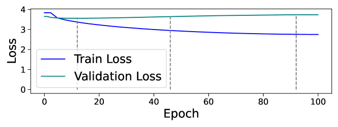
Figure 12: Target model (GPT-2) loss during overtraining on WikiText-2 dataset. We pick GPT-2_E12, GPT-2_E23, GPT-2_E46, GPT-2_E92 as target models to audit corresponding to the gray dashed lines.

Generator. The ${\mathcal{G}}$ is a GPT-2 fine-tuned using a CLM task on dataset $D_{G}$, a subset of $D_{f}$. To create synthetic samples with ${\mathcal{G}}$, we use top-$p$ sampling Holtzman et al. (2019) method in an auto-regressive manner while keeping the generated sequence length fixed at 64 tokens. To make ${\mathcal{G}}$ generate samples less like the real members it learned from (and hopefully, more like real non-members), we introduce more randomness in the generation process in the following manner. First, we set the top_p parameter that determines the probability cutoff for the selection of a pool of tokens to sample from to the value of 1. We also choose a top_k value of 200, controlling the number of available tokens for sampling after applying top_p filtering. In addition, we balance the value of top_k, making it not too small to avoid repetitive generated texts but also not too large to maintain the quality. Finally, we fix the temperature parameter that controls the randomness in the softmax function at one. Indeed, a larger value increases the entropy of the distribution over tokens resulting in a more diverse generated text.

However, the quality of synthetic text depends on the prompts used. Indeed, some prompts, such as $"<|endoftext|>"$, can lead to poor results. To mitigate this issue, we split the $D_{G}$ dataset into two parts: $D_{G}^{train}$ and $D_{G}^{prompt}$. ${\mathcal{G}}$ is fine-tuned on $D_{G}^{train}$, while $D_{G}^{prompt}$ is used for generating prompts. Numerically, the size of the $D_{G}^{train}$ is $44\%$ of the $D_{f}$ and the size of $D_{G}^{prompt}$ is $23\%$ of $D_{f}$. During generation, we sample from $D_{G}^{prompt}$, which is a sequence of length 64. We feed the prompt into the generator and request the generator to generate a suffix of equivalent length. In our experiments, for each prompt, we make 5 synthetic samples, supplying a sufficient number of synthetic non-member samples for different parts of the pipeline of PANORAMIA, including training the helper model, and constructing $D^{\textrm{tr}}_{\textrm{out}}$, $D^{\textrm{te}}_{\textrm{out}}$. Overall, we generate 62524 synthetic samples out of which we use 41968 of them for training the helper model and keep the rest for audit purposes. Note that this generation approach does not inherently favor our audit scheme, and shows how PANORAMIA can leverage existing, public generative models with fine tuning to access high-quality generators at reasonable training cost.

Baseline & MIA. For both the baseline and PANORAMIA classifiers, we employ a GPT-2 based sequence classification model. In this setup, GPT-2 extracts features (i.e., hidden vectors) directly from the samples. We concatenate a vector of features extracted using the helper $h$ (for the baseline) or target model $f$ (for the MIA) to this representation. This vector of features is the loss sequence produced in a CLM task for the respective model. These two sets of extracted features are then concatenated before being processed through a feed-forward layer to generate the logit values required for binary classification (distinguishing between members and non-members).

For both the baseline and PANORAMIA classifiers, the training and validation sets consist of 12000 and 2000 samples, respectively, with equal member non-member distribution. The test set consists of 10000 samples, in which the actual number of members and non-members that ended up in the test set depends on the Bernoulli samples in the auditing game. The helper model is fine-tuned for $40$ epochs on synthetic samples and we pick the model that has the lowest validation loss throughout training, generalizing well.

As the GPT-2 component of the classifiers can effectively minimize training loss without achieving strong generalization, regularization is applied to the classifier using weight decay. Additionally, the optimization process is broken into two phases. In the first phase, we exclusively update the parameters associated with the target (in PANORAMIA) or helper model (in the baseline) to ensure that this classifier has the opportunity to focus on these specific features. In the second phase, we optimize the entire model as usual. We train the baseline or MIA with at least 5 seeds, in which the randomness is over the randomness of training (such as initialization of the model, and batch sampling). We select models throughout training with the best validation accuracy. Subsequently, we pick the model with the best validation accuracy among models with different seeds and produce the audit result on the auditing test set with the selected model.

B.3 Tabular data

Target $f$ and the helper model $\mathbf{h.}$ The Target $f$ and the helper $h$ model are both Multi-Layer Perceptron with four hidden layers containing 150, 100, 50, and 10 neurons respectively. Both models are trained using a learning rate of 0.0005 over 100 training epochs. In the generalized case and to obtain the embedding, we retain the model’s parameters that yield the lowest loss on a validation set, which typically occurs at epoch 10. For the overfitted scenario, we keep the model’s state after the 100 training epochs.

Generator. We use the MST method McKenna et al. (2021) which is a differentialy-private method to generate synthetic data. However, as we do not need Differential Privacy for data generation we simply set the value for $\varepsilon$ to $1000$. Synthetic data generators can sometimes produce bad-quality samples. Those out-of-distribution samples can affect our audit process (the detection between real and synthetic data being due to bad quality samples rather than privacy leakage). To circumvent this issue, we train an additional classifier to distinguish between real data from $D_{G}$ and additional synthetic data (not used in the audit). We use this classifier to remove from the audit data synthetic data synthetic samples predicted as synthetic with high confidence.

Baseline and MIA. To distinguish between real and synthetic data, we use the Gradient Boosting model and conduct a grid search to find the best hyperparameters.

B.4 Comparison with Privacy Auditing with One (1) Training Run: Experimental Details

We implement the black-box auditor version of O(1) approach Steinke et al. (2023). This method assigns a membership score to a sample based on its loss value under the target model. They also subtract the sample’s loss under the initial state (or generally, a randomly initialized model) of the target model, helping to distinguish members from non-members even more. In our instantiation of the O(1) approach, we only consider the loss of samples on the final state of the target model. Moreover, in their audit, they choose not to guess the membership of every sample. This abstention has an advantage over making wrong predictions as it does not increase their baseline. Roughly speaking, their baseline is the total number of correct guesses achieved by employing a randomized response $(\epsilon,0)$ mechanism, for those samples that O(1) auditor opts to predict. We incorporate this abstention approach in our implementation by using two thresholds, $t_{+}$ and $t_{-}$. More precisely, samples with scores below $t_{+}$ are predicted as members, those above $t_{-}$ as non-members, and the rest are abstained from prediction. We check all possible combinations of $t_{+}$ and $t_{-}$ and report the highest $\epsilon$ among them, following a common practice Zanella-Béguelin et al. (2022); Maddock et al. (2023). We also set $\delta$ to 0 and use a confidence interval of 0.05 in their test. In PANORAMIA, for each hypothesis test (whether for $c_{\textrm{lb}}$ or $\{c\!+\!\epsilon\}_{\textrm{lb}}$), we stick to a 0.025 confidence interval for each one, adding up to an overall confidence level of 0.05. Furthermore, the audit set of O(1) is the same as the audit set of PANORAMIA.

B.5 Comparison with MIA on RM; RN: Experimental details on tabular

In order to proceed with the comparison of PANORAMIA with a variant of PANORAMIA in which we use real data instead of synthetic data, we need a significant number of real non-member observations. Due to the limited size of the adult dataset ($\approx 30k$ observations), we train the target model $f$ on only half of the dataset and use the remaining half to train and evaluate the MIA.

Appendix C Results: More experiments and Detailed Discussion

C.1 Baseline Strength Evaluation on Text and Tabular datasets

Baseline model	$c_{lb}$
CIFAR-10 Baseline$D_{h}^{\text{tr}}=\text{real, resnet101}$	2.16
CIFAR-10 Baseline$D_{h}^{\text{tr}}=\text{imgnet}$	1.10
CIFAR-10 Baselineno helper	1.15
CIFAR-10 Baseline$D_{h}^{\text{tr}}=\text{real, WRN}$	2.37
CIFAR-10 Baseline$D_{h}^{\text{tr}}=\text{gen, WRN}$	2.508
CelebA Baseline$D_{h}^{\text{tr}}=\text{gen}$	2.03
CelebA Baseline$D_{h}^{\text{tr}}=\text{real}$	1.67
CelebA Baselineno helper	0.91
WikiText-2 Baseline$D_{h}^{\text{tr}}=\text{gen}$	2.61
WikiText-2 Baseline$D_{h}^{\text{tr}}=\text{real}$	2.59
WikiText-2 Baselineno helper	2.34
Adult Baseline$D_{h}^{\text{tr}}=\text{gen}$	2.34
Adult Baseline$D_{h}^{\text{tr}}=\text{real}$	2.18
Adult Baselineno helper	2.01

Table 6: Baseline evaluation with different helper model scenarios, where WRN is Wide-ResNet-28-2 helper model architecture (in the case of CIFAR10 baseline).

The basis of our audit directly depends on how well our baseline classifier distinguishes between real member data samples and synthetic non-member data samples generated by our generative model. To assess the strength of the baseline classifier, we train the baseline’s helper model $h$ on two datasets, synthetic data, and real non-members. We also train a baseline without any helper model. This enables us to identify which setup allows the baseline classifier to distinguish the member and non-member data the best in terms of the highest $c_{lb}$ value ($c_{lb}$ is reported for each case in table 6). For initial analysis, we keep a sub-set of real data as non-members to train a helper model with them, for conducting this ablation study on the baseline. Our experiments confirm that the baseline with loss values from a helper model trained on synthetic data performs better compared to a helper model trained on real non-member data. This confirms the strength of our framework in terms of not having a dependency of using real non-members. Therefore, we choose this setting for our baseline helper model. In addition, we also experiment with different helper model architectures in the case of CIFAR10, looking for the best baseline performance among them.

For each data modality setting, we also train the baseline classifier on an increasing dataset size of real member and synthetic non-member data points to gauge the trend of the baseline performance as the training dataset size increases (see Figure 2 and Figure LABEL:fig:baseline-othermodalities-eval). This experiment allows us to aim for a worst-case empirical lower bound on how close the generated non-member data is to the real member data distribution, i.e. what would be the largest $c_{\textrm{lb}}$ we can reach as we increase the training set size. Subsequently, we can compare the $c_{\textrm{lb}}$ reported in table 4 (corresponding to the vertical dashed lines in Figure 2 and Figure LABEL:fig:baseline-othermodalities-eval) to the largest $c_{\textrm{lb}}$ we can achieve in this experiment. In the following, we explain why we choose that number of training samples for our baseline in the main results.

On the WikiText dataset, we augment the baseline’s training set by shortening the validation and test sets (from 1000 to 500 and from 10000 to 2000, respectively). This modification accounts for the mismatch between the $c_{\textrm{lb}}$ at the vertical dashed line in Figure LABEL:subfig:nlp_plateau and the reported one in Table 4. Nevertheless, the maximum average $c_{\textrm{lb}}$ attained on our largest training set for the baseline (represented by the horizontal dashed line in Figure LABEL:subfig:nlp_plateau) is 3.66, which is still lower than 3.78, the one reported in Table 4.

Due to dataset size constraints in practicality, in terms of how much real member data is available, the train dataset size for our MIA and baseline where the performance of the baseline in terms of $c_{lb}$ is the highest. This accounts for how much data we have in terms of member data for the target model, and the split we account for while training the respective generative models, as well as the real members test data used to evaluate the MIA and baseline. These data constraints lead us to choose the train dataset size as shown by the vertical line in Figure 2 and Figure LABEL:fig:baseline-othermodalities-eval. Hence the final values reported in Table 3 are on these corresponding data sizes. It is also important to note that the MIA is expected to show similar behavior if we use a larger dataset size for training if it was available.

The experiments are repeated ten times to account for randomness during training (e.g., initialization, sampling in batches) and report the results over a $95\%$ confidence interval.

C.2 Further Analysis on General Auditing Results

The value of $\tilde{\epsilon}$ for each target model is the gap between its corresponding dashed line and the baseline one in Figure LABEL:fig:eval:comparison. This allows us to compute values of $\tilde{\epsilon}$ reported in Table 4. It is also interesting to note that the maximum value of $\{c\!+\!\epsilon\}_{\textrm{lb}}$ typically occurs at low recall. Even if we do not use the same metric (precision-recall as opposed to TPR at low FPR) this is coherent with the findings from Carlini et al. (2022b). We can detect more privacy leakage (higher $\{c\!+\!\epsilon\}_{\textrm{lb}}$ which leads to higher $\tilde{\epsilon}$) when making a few confident guesses about membership rather than trying to maximize the number of members found (i.e., recall). Figure LABEL:fig:preds_comparison, decomposes the precision in terms of the number of true positives and the number of predictions for a direct mapping to the propositions 1 and 2. These are non-negligible values of privacy leakage, even through the true value is likely much higher.

C.3 PANORAMIA in cases of no privacy leakage

As illustrated in Figure LABEL:fig:gpt2_privacy_recall, there exist instances in whch the $c_{\textrm{lb}}$ is as large or even larger than $\{c\!+\!\epsilon\}_{\textrm{lb}}$ (such as in GPT-2_E12). This implies that, under certain conditions, the baseline could outperform the MIA in PANORAMIA. We can see three possible reasons for this behavior. (1) The synthetic data might not be of high enough quality. If there is an evident distinction between real and synthetic samples, the baseline cannot be fooled reducing the power of our audit. (2) The MIA in PANORAMIA is not powerful enough. (3) The target model’s privacy leakage is indeed low. For GPT-2_E92 and GPT-2_E46 in Figure LABEL:fig:gpt2_privacy_recall, we can claim that given the target model’s leakage level, the synthetic data and the MIA can perform the audit to a non-negligible power. For GPT-2_12, we need to examine the possible reasons more closely. Focusing on generated data, in the ideal case we would like the synthetic data to behave just like real non-member data on Figure LABEL:subfig:lossdist-gpt-2E12. If this was the case, $\{c\!+\!\epsilon\}_{\textrm{lb}}$ would go up (since the MIA uses this loss to separate members and non-members). Nonetheless, predicting changes in $c_{\textrm{lb}}$ remains challenging, as analogous loss distributions do not guarantee indistinguishability between data points themselves (also, we cannot necessarily predict how the loss distribution changes under the helper model $h$ in Figure LABEL:subfig:lossdist-h). Hence, reason (1) which corresponds to low generative data quality, seems to be a factor in the under-performance of PANORAMIA. Moreover, in the case GPT-2_12, we observe that real members and non-members have very similar loss distributions. Hence, factor (2) also seems to be at play, and a stronger MIA that does not rely exclusively on the plot may increase auditing power. Finally, the helper model $h$ seems to have a more distinct loss distribution when compared to GPT-2_12. If the MIA had access to both target and helper models, we would expect $\{c\!+\!\epsilon\}_{\textrm{lb}}$ to at least match $c_{\textrm{lb}}$.

C.4 Failure of PANORAMIA in the case of tabular data

Our proposed method PANORAMIA can suffer some interesting failure cases that can be well illustrated with tabular data. Figure LABEL:fig:fail_privacy illustrates an interesting case of failure observed during one of our experiments with the generative model being trained on only part of the target model $f$ training set. First, by taking a closer look at the precision-recall curve of both the baseline (blue) and PANORAMIA ’s MIA for MLP_E100 on figure LABEL:fig:fail_precision, we notice that the precision-recall curve of the MIA is mostly above the baseline. However, the baseline has higher maximum precision values at extremely low recall. As a result, we can see in Figure LABEL:fig:fail_privacy that the maximum value for $(c+\varepsilon)_{lb}$ is lower than $c_{lb}$ leading to failure in measuring privacy leakage. This is due to our independent selection of recall thresholds, choosing heuristically the highest value.

The high precision at low recall in the baseline illustrates the fact that some real data can easily be distinguished from the synthetic ones. Instead of poor quality synthetic data as exposed in C.3, we are dealing with real observation that are actually “looking to real”. Investigating those observations reveals that they have extreme or rare values in one of their features. Indeed, the Adult dataset contains some extreme values (e.g., in the capital_gain column), such extreme values are rarely reproduced by the generative model. This leads to the baseline accurately predicting such observations as real with high confidence that translates into a high $c_{lb}$. This behavior is the opposite of what we generally expect in MIA in which extreme values are usually more vulnerable to MIA Carlini et al. (2022b). This is a potential drawback of our auditing scheme, while the presence of extreme or rare values in the dataset usually allows for good auditing results it can have a negative impact on PANORAMIA’s success.

C.5 Privacy Auditing of Overfitted ML Models

Methodology. Varying the number of training epochs for the target model to induce overfitting is known to be a factor in privacy loss Yeom et al. (2018); Carlini et al. (2022a). As discussed in Section 5.2, since these different variants of target models share the same dataset and task, PANORAMIA can compare them in terms of privacy leaking.

To verify if PANORAMIA will indeed attribute a higher value of $\tilde{\epsilon}$ to more overfitted models, we train our target models for varying numbers of training epochs. The final train and test accuracies are reported in Table 2. For GPT-2 (as a target model), we report the train and validation loss as a measure of overfitting in Figure 12. Figures LABEL:fig:gpt_losses and LABEL:fig:celeb_losses show how the gap between member data points (i.e., data used to train the target models) and non-member data points (both real as well as generated non-members) increases as the degree of overfitting increases, in terms of loss distributions. We study the distribution of losses since these are the features extracted from the target model $f$ or helper model $h$, to pass respectively to PANORAMIA and the baseline classifier. The fact that the loss distributions of member data become more separable from non-member data for more overfitted models is a sign that the corresponding target model could leak more information about its training data. We thus run PANORAMIA on each model, hereafter presenting the results obtained.

Results. In Figure LABEL:fig:eval:comparison_precision, we observe that more training epochs (i.e., more overfitting) lead to better precision-recall trade-offs and higher maximum precision values. Our results are further confirmed by Figure LABEL:fig:preds_comparison with PANORAMIA being able to capture the number of member data points better than the baseline $b$.

In Table 4, we further demonstrate that our audit output $\tilde{\epsilon}$ orders the target models in terms of privacy leakage: higher the degree of overfitting, more memorization and hence a higher $\tilde{\epsilon}$ returned by PANORAMIA. From our experiments, we consistently found that as the number of epochs increased, the value of $\tilde{\epsilon}$ also increased. For instance, in the WikiText-2 dataset, since we observe $\{c\!+\!\epsilon\}_{\textrm{lb}}^{\text{GPT-2\_E92}}>\{c\!+\!\epsilon\}_{\textrm{lb}}^{\text{GPT-2\_E46}}>\{c\!+\!\epsilon\}_{\textrm{lb}}^{\text{GPT-2\_E12}}$, we would have $\{c\!+\!\epsilon\}_{\textrm{lb}}^{\text{GPT-2\_E92}}-c_{\textrm{lb}}>\{c\!+\!\epsilon\}_{\textrm{lb}}^{\text{GPT-2\_E46}}-c_{\textrm{lb}}>\{c\!+\!\epsilon\}_{\textrm{lb}}^{\text{GPT-2\_E12}}-c_{\textrm{lb}}$, which leads to $\tilde{\epsilon}_{\text{GPT-2\_E92}}>\tilde{\epsilon}_{\text{GPT-2\_E46}}>\tilde{\epsilon}_{\text{GPT-2\_E12}}$. Our experiment is coherent with the intuition that more training epochs lead to more over-fitting, leading to more privacy leakage measured with a higher value of $\tilde{\epsilon}$.

C.6 Privacy Auditing of Differentially-Private ML Models

Methodology. We evaluate the performance of PANORAMIA on differentially-private ResNet-18 and Wide-ResNet-16-4 models on the CIFAR10 dataset under different target privacy budgets ($\epsilon$) with $\delta=10^{-5}$ and the non-private ($\epsilon=\infty$) cases. The models are trained using the DP-SGD algorithm (Abadi et al., 2016) using Opacus (Yousefpour et al., 2021), which we tune for the highest train accuracy on learning rate $lr$, number of epochs $e$, batch size $bs$ and maximum $\ell_{2}$ clipping norm (C) for the largest final accuracy. The noise multiplier $\sigma$ is computed given $\epsilon$, number of epochs and batch size. Both PANORAMIA and O(1) (Steinke et al., 2023) audits privacy loss with pure $\epsilon$-DP analysis.

Results. Tables 7 and 8 summarizes the auditing results of PANORAMIA on different DP models. For ResNet-18, we observe that at $\epsilon=1,2,4,6$ (more private models) PANORAMIA detects no privacy loss, whereas at higher values of $\epsilon=10,15,20$ (less private models) and $\epsilon=\infty$ (a non-private model) PANORAMIA detects an increasing level of privacy loss with $\tilde{\epsilon}_{\epsilon=10}<\tilde{\epsilon}_{\epsilon=15}<\tilde{\epsilon}_{\epsilon=20}<\tilde{\epsilon}_{\epsilon=\infty}$, suggesting a higher value of $\epsilon$ correspond to higher $\tilde{\epsilon}$. We observe a similar pattern with Wide-ResNet-16-4, in which no privacy loss is detected at $\epsilon=1,2$ and higher privacy loss is detected at $\epsilon=10,15,20,\infty$. We also compare the auditing performance of PANORAMIA with that of O(1) (Steinke et al., 2023), with the conclusion drawn by these two methods being comparable. For both ResNet-18 and Wide-ResNet-16-4, O(1) reports values close to 0 (almost a random guess between members and non-members) for $\epsilon<10$ DP models, and higher values for $\epsilon=10,15,20,\infty$ DP models. The results suggest that PANORAMIA is potentially an effective auditing tool for DP models that has comparable performance with O(1) and can generalize to different model structures.

Target model	Audit	$\mathbf{c_{lb}}$	$\mathbf{\varepsilon+c_{lb}}$	$\mathbf{\tilde{\varepsilon}}$	$\mathbf{\varepsilon}$
ResNet18 $\epsilon=\infty$	PANORAMIA RM;GN	2.508	3.6698	1.161	-
	O (1) RM;RN	-	-	-	1.565
ResNet18 $\epsilon=20$	PANORAMIA RM;GN	2.508	3.6331	1.125	-
	O (1) RM;RN	-	-	-	1.34
ResNet18 $\epsilon=15$	PANORAMIA RM;GN	2.508	3.5707	1.062	-
	O (1) RM;RN	-	-	-	1.22
ResNet18 $\epsilon=10$	PANORAMIA RM;GN	2.508	2.8	0.3	-
	O (1) RM;RN	-	-	-	0.14
ResNet18 $\epsilon=6$	PANORAMIA RM;GN	2.508	1.28	0	-
	O (1) RM;RN	-	-	-	0.049
ResNet18 $\epsilon=4$	PANORAMIA RM;GN	2.508	1.989	0	-
	O (1) RM;RN	-	-	-	0
ResNet18 $\epsilon=2$	PANORAMIA RM;GN	2.508	2.065	0	-
	O (1) RM;RN	-	-	-	0.08
ResNet18 $\epsilon=1$	PANORAMIA RM;GN	2.508	1.982	0	-
	O (1) RM;RN	-	-	-	0

Table 7: Privacy audit of ResNet18 under different values of $\epsilon$-Differential Privacy using PANORAMIA and O(1) auditing frameworks, in which $RM$ is for real member, $RN$ for real non-member and $GN$ for generated (synthetic) non-members.

Target model	Audit	$\mathbf{c_{lb}}$	$\mathbf{\varepsilon+c_{lb}}$	$\mathbf{\tilde{\varepsilon}}$	$\mathbf{\varepsilon}$
WRN-16-4 $\epsilon=\infty$	PANORAMIA RM;GN	2.508	2.9565	0.448	-
	O (1) RM;RN	-	-	-	0.6408
WRN-16-4 $\epsilon=20$	PANORAMIA RM;GN	2.508	2.95161	0.4436	-
	O (1) RM;RN	-	-	-	0.5961
WRN-16-4 $\epsilon=15$	PANORAMIA RM;GN	2.508	2.91918	0.411	-
	O (1) RM;RN	-	-	-	0.5774
WRN-16-4 $\epsilon=10$	PANORAMIA RM;GN	2.508	2.83277	0.3247	-
	O (1) RM;RN	-	-	-	0.171
WRN-16-4 $\epsilon=2$	PANORAMIA RM;GN	2.508	2.2096	0	-
	O (1) RM;RN	-	-	-	0
WRN-16-4 $\epsilon=1$	PANORAMIA RM;GN	2.508	1.15768	0	-
	O (1) RM;RN	-	-	-	0

Table 8: Privacy audit of Wide ResNet16-4 under different values of $\epsilon$-Differential Privacy (DP) using PANORAMIA and O(1) auditing frameworks, where $RM$ is for real member, $RN$ for real non-member and $GN$ for generated (synthetic) non-members.

Discussion.

We observe that the auditing outcome ($\tilde{\epsilon}$ values for PANORAMIA and $\epsilon$ for O(1)) can be different for DP models with the same $\epsilon$ values (Table 9). We hypothesize that the auditing results may relate more to level of overfitting than the target $\epsilon$ values in trained DP models. The difference between train and test accuracies could be a possible indicator that has a stronger relationship with the auditing outcome. We also observe that O(1) shows a faster increase in $\epsilon$ for DP models with higher targeted $\epsilon$ values. We believe it depends on the actual ratio of the correct and total number of predicted samples, since O(1) considers both true positives and true negatives while PANORAMIA considers true positives only. We leave these questions for future work.

Target model	Audit	$\mathbf{c_{lb}}$	$\mathbf{\varepsilon+c_{lb}}$	$\mathbf{\tilde{\varepsilon}}$	$\mathbf{\varepsilon}$	Train Acc	Test Acc	Diff(Train-Test Acc)
ResNet18-eps-20	PANORAMIA RM;GN	2.508	3.63	1.06	-	71.82	67.12	4.70
	O (1) RM;RN	-	-	-	1.22	-	-	-
	PANORAMIA RM;GN	2.508	2.28	0	-	71.78	68.08	3.70
	O (1) RM;RN	-	-	-	0.09	-	-	-
ResNet18-eps-15	PANORAMIA RM;GN	2.508	3.63	1.13	-	69.01	65.7	3.31
	O (1) RM;RN	-	-	-	1.34	-	-	-
	PANORAMIA RM;GN	2.508	1.61	0		66.68	69.30	2.62
	O (1) RM;RN	-	-	-	0.08	-	-	-

Table 9: DP models with the same $\epsilon$ values can have different auditing outcomes.

Appendix D Extended Related Work

Most related privacy auditing works measure the privacy of an ML model by lower-bounding its privacy loss. This usually requires altering the training pipeline of the ML model, either by injecting canaries that act as outliers Carlini et al. (2019) or by using data poisoning attack mechanisms to search for worst-case memorization Jagielski et al. (2020); Nasr et al. (2021). MIAs are also increasingly used in privacy auditing, to estimate the degree of memorization of member data by an ML algorithm by resampling the target algorithm $\mathcal{M}$ to bound $\frac{P(M|in)}{P(M|out)}$ Jayaraman & Evans (2019). The auditing procedure usually involves searching for optimal neighboring datasets $D,D^{\prime}$ and sampling the DP outputs $\mathcal{M}(D),\mathcal{M}(D^{\prime})$, to get a Monte Carlo estimate of $\epsilon$. This approach raises important challenges. First, existing search methods for neighboring inputs, involving enumeration or symbolic search, are impossible to scale to large datasets, making it difficult to find optimal dataset pairs. In addition, Monte Carlo estimation requires up to thousands of costly model retrainings to bound $\epsilon$ with high confidence. Consequently, existing approaches for auditing ML models predominantly require the re-training of ML models for every (batch of) audit queries, which is computationally expensive in large-scale systems Jagielski et al. (2020); Zanella-Béguelin et al. (2022); Lu et al. (2023). This makes privacy auditing computationally expensive and gives an estimate by averaging over models, which might not reflect the true guarantee of a specific pipeline deployed in practice.

Nonetheless, improvements to auditing have been made in a variety of directions. For example, Nasr et al. (2023) and Maddock et al. (2023) have taken advantage of the iterative nature of DP-SGD, auditing individual steps to understand the privacy of the end-to-end algorithm.  Andrew et al. (2023) leverage the fact that analyzing MIAs for non-member data does not require re-running the algorithm. Instead, it is possible to re-sample the non-member data point: if the data points are i.i.d. from an asymptotically Gaussian distribution with mean zero and variance $1/d$, this enables a closed-form analysis of the non-member case.

Recently, Steinke et al. (2023) proposed a novel scheme for auditing differential privacy with $O(1)$ training rounds. This approach enables privacy audits using multiple training examples from the same model training, if examples are included in training independently (which requires control over the training phase, and altering the target model). They demonstrate the effectiveness of this new approach on DP-SGD, in which they achieve meaningful empirical privacy lower bounds by training only one model, whereas standard methods would require training hundreds of models. Our work builds on the theory from Steinke et al. (2023), but removes the need from controlling and altering the training phase, as PANORAMIA requires no retraining.

References

- Abadi et al. (2016) Abadi, M., Chu, A., Goodfellow, I., McMahan, H. B., Mironov, I., Talwar, K., and Zhang, L. Deep learning with differential privacy. In Proceedings of the 2016 ACM SIGSAC conference on computer and communications security, pp. 308–318, 2016.
- Andrew et al. (2023) Andrew, G., Kairouz, P., Oh, S., Oprea, A., McMahan, H. B., and Suriyakumar, V. One-shot empirical privacy estimation for federated learning, 2023.
- Balle et al. (2022) Balle, B., Cherubin, G., and Hayes, J. Reconstructing training data with informed adversaries, 2022.
- Becker & Kohavi (1996) Becker, B. and Kohavi, R. Adult. UCI Machine Learning Repository, 1996. DOI: https://doi.org/10.24432/C5XW20.
- Carlini et al. (2019) Carlini, N., Liu, C., Erlingsson, Ú., Kos, J., and Song, D. The secret sharer: Evaluating and testing unintended memorization in neural networks. In 28th USENIX Security Symposium (USENIX Security 19), pp. 267–284, 2019.
- Carlini et al. (2021) Carlini, N., Tramer, F., Wallace, E., Jagielski, M., Herbert-Voss, A., Lee, K., Roberts, A., Brown, T., Song, D., Erlingsson, U., et al. Extracting training data from large language models. In 30th USENIX Security Symposium (USENIX Security 21), 2021.
- Carlini et al. (2022a) Carlini, N., Chien, S., Nasr, M., Song, S., Terzis, A., and Tramer, F. Membership inference attacks from first principles. In 2022 2022 IEEE Symposium on Security and Privacy (SP) (SP), pp. 1519–1519, Los Alamitos, CA, USA, may 2022a. IEEE Computer Society. doi: 10.1109/SP46214.2022.00090. URL https://doi.ieeecomputersociety.org/10.1109/SP46214.2022.00090.
- Carlini et al. (2022b) Carlini, N., Chien, S., Nasr, M., Song, S., Terzis, A., and Tramer, F. Membership inference attacks from first principles. In 2022 IEEE Symposium on Security and Privacy (SP), pp. 1897–1914. IEEE, 2022b.
- Choquette-Choo et al. (2020) Choquette-Choo, C. A., Tramer, F., Carlini, N., and Papernot, N. Label-only membership inference attacks, 2020. URL https://arxiv.org/abs/2007.14321.
- Dong et al. (2019) Dong, J., Roth, A., and Su, W. J. Gaussian differential privacy. arXiv preprint arXiv:1905.02383, 2019.
- Dwork et al. (2006) Dwork, C., McSherry, F., Nissim, K., and Smith, A. Calibrating noise to sensitivity in private data analysis. In Theory of cryptography conference. Springer, 2006.
- He et al. (2015) He, K., Zhang, X., Ren, S., and Sun, J. Deep residual learning for image recognition, 2015.
- Holtzman et al. (2019) Holtzman, A., Buys, J., Du, L., Forbes, M., and Choi, Y. The curious case of neural text degeneration. arXiv preprint arXiv:1904.09751, 2019.
- Jagielski et al. (2020) Jagielski, M., Ullman, J., and Oprea, A. Auditing differentially private machine learning: How private is private sgd? Advances in Neural Information Processing Systems, 33:22205–22216, 2020.
- Jayaraman & Evans (2019) Jayaraman, B. and Evans, D. E. Evaluating differentially private machine learning in practice. In USENIX Security Symposium, 2019.
- Kairouz et al. (2015) Kairouz, P., Oh, S., and Viswanath, P. The composition theorem for differential privacy. In International conference on machine learning. PMLR, 2015.
- Karras et al. (2020) Karras, T., Aittala, M., Hellsten, J., Laine, S., Lehtinen, J., and Aila, T. Training generative adversarial networks with limited data, 2020.
- Krizhevsky et al. (2009) Krizhevsky, A., Hinton, G., et al. Learning multiple layers of features from tiny images. Technical report, University of Toronto, 2009.
- Liu et al. (2015) Liu, Z., Luo, P., Wang, X., and Tang, X. Deep learning face attributes in the wild. In Proceedings of International Conference on Computer Vision (ICCV), December 2015.
- Lu et al. (2023) Lu, F., Munoz, J., Fuchs, M., LeBlond, T., Zaresky-Williams, E., Raff, E., Ferraro, F., and Testa, B. A general framework for auditing differentially private machine learning, 2023.
- Maddock et al. (2023) Maddock, S., Sablayrolles, A., and Stock, P. Canife: Crafting canaries for empirical privacy measurement in federated learning, 2023.
- McKenna et al. (2021) McKenna, R., Miklau, G., and Sheldon, D. Winning the nist contest: A scalable and general approach to differentially private synthetic data. arXiv preprint arXiv:2108.04978, 2021.
- Merity et al. (2016) Merity, S., Xiong, C., Bradbury, J., and Socher, R. Pointer sentinel mixture models. arXiv preprint arXiv:1609.07843, 2016.
- Nasr et al. (2021) Nasr, M., Songi, S., Thakurta, A., Papernot, N., and Carlin, N. Adversary instantiation: Lower bounds for differentially private machine learning. In 2021 IEEE Symposium on Security and Privacy (SP), pp. 866–882, 2021. doi: 10.1109/SP40001.2021.00069.
- Nasr et al. (2023) Nasr, M., Hayes, J., Steinke, T., Balle, B., Tramèr, F., Jagielski, M., Carlini, N., and Terzis, A. Tight auditing of differentially private machine learning, 2023.
- O’Shea & Nash (2015) O’Shea, K. and Nash, R. An introduction to convolutional neural networks, 2015.
- Radford et al. (2019) Radford, A., Wu, J., Child, R., Luan, D., Amodei, D., Sutskever, I., et al. Language models are unsupervised multitask learners. OpenAI blog, 1(8):9, 2019.
- Shokri et al. (2017) Shokri, R., Stronati, M., Song, C., and Shmatikov, V. Membership inference attacks against machine learning models, 2017.
- Song & Mittal (2020) Song, L. and Mittal, P. Systematic evaluation of privacy risks of machine learning models, 2020. URL https://arxiv.org/abs/2003.10595.
- Steinke et al. (2023) Steinke, T., Nasr, M., and Jagielski, M. Privacy auditing with one (1) training run, 2023.
- Wasserman & Zhou (2010) Wasserman, L. and Zhou, S. A statistical framework for differential privacy. Journal of the American Statistical Association, 2010.
- Yeom et al. (2018) Yeom, S., Giacomelli, I., Fredrikson, M., and Jha, S. Privacy risk in machine learning: Analyzing the connection to overfitting. In 2018 IEEE 31st computer security foundations symposium (CSF), pp. 268–282. IEEE, 2018.
- Yousefpour et al. (2021) Yousefpour, A., Shilov, I., Sablayrolles, A., Testuggine, D., Prasad, K., Malek, M., Nguyen, J., Ghosh, S., Bharadwaj, A., Zhao, J., Cormode, G., and Mironov, I. Opacus: User-friendly differential privacy library in PyTorch. arXiv preprint arXiv:2109.12298, 2021.
- Zagoruyko & Komodakis (2017) Zagoruyko, S. and Komodakis, N. Wide residual networks, 2017.
- Zanella-Béguelin et al. (2022) Zanella-Béguelin, S., Wutschitz, L., Tople, S., Salem, A., Rühle, V., Paverd, A., Naseri, M., Köpf, B., and Jones, D. Bayesian estimation of differential privacy, 2022.