Fourier Circuits in Neural Networks: Unlocking the Potential of Large Language Models in Mathematical Reasoning and Modular Arithmetic

In the evolving landscape of machine learning, a pivotal challenge lies in deciphering the internal representations harnessed by neural networks and Transformers. Building on recent progress toward comprehending how networks execute distinct target functions, our study embarks on an exploration of the underlying reasons behind networks adopting specific computational strategies. We direct our focus to the complex algebraic learning task of modular addition involving $k$ inputs. Our research presents a thorough analytical characterization of the features learned by stylized one-hidden layer neural networks and one-layer Transformers in addressing this task.

A cornerstone of our theoretical framework is the elucidation of how the principle of margin maximization shapes the features adopted by one-hidden layer neural networks. Let $p$ denote the modulus, $D_{p}$ denote the dataset of modular arithmetic with $k$ inputs and $m$ denote the network width. We demonstrate that a neuron count of $m\geq 2^{2k-2}\cdot(p-1)$, these networks attain a maximum $L_{2,k+1}$-margin on the dataset $D_{p}$. Furthermore, we establish that each hidden-layer neuron aligns with a specific Fourier spectrum, integral to solving modular addition problems.

By correlating our findings with the empirical observations of similar studies, we contribute to a deeper comprehension of the intrinsic computational mechanisms of neural networks. Furthermore, we observe similar computational mechanisms in the attention matrix of the Transformer. This research stands as a significant stride in unraveling their operation complexities, particularly in the realm of complex algebraic tasks.

1 Introduction

The field of artificial intelligence has experienced a significant transformation with the development of large language models (LLMs), particularly through the introduction of the Transformer architecture. This advancement has revolutionized approaches to challenging tasks in natural language processing, notably in machine translation [67, 27] and text generation [52]. Consequently, models e.g., BERT [19], PaLM [16], LLaMA 2[86], ChatGPT [64], GPT4 [65] and so on, have become predominant in NLP.

Central to this study is the question of how these advanced models transcend mere pattern recognition to engage in what appears to be logical reasoning and problem-solving. This inquiry is not purely academic; it probes the core of “understanding” in artificial intelligence. While LLMs, such as GPT, demonstrate remarkable proficiency in human-like text generation, their capability in comprehending and processing mathematical logic is a topic of considerable debate.

This line of investigation is crucial, given AI’s potential to extend beyond text generation into deeper comprehension of complex subjects. Mathematics, often seen as the universal language, presents a uniquely challenging domain for these models [95]. Our research aims to determine if Transformers, noted for their NLP efficiency, can also demonstrate an intrinsic understanding of mathematical operations and reasoning.

A recent surprising study of mathematical operations learning, [66] train Transformers on small algorithmic datasets, e.g., $a_{1}+a_{2}\mod p$ and we let $p$ be a prime number, and show the “grokking” phenomenon, where models abruptly transition from bad generalization to perfect generalization after a large number of training steps. Nascent studies, such as those by [60], empirically reveal that Transformers can solve modular addition using Fourier-based circuits. They found that the Transformers trained by Stochastic Gradient Descent (SGD) not only reliably compute $a_{1}+a_{2}\mod p$, but also that the networks consistently employ a specific geometric algorithm. This algorithm, which involves composing integer rotations around a circle, indicates an inherent comprehension of modular arithmetic within the network’s architecture. The algorithm relies on this identity: for any $a_{1},a_{2}$ and $\zeta\in\mathbb{Z}_{p}\backslash\{0\}$, the following two quantities are equivalent

• $(a_{1}+a_{2})\bmod p$

• $\underset{c\in\mathbb{Z}_{p}}{\arg\max}\{\cos({2\pi\zeta(a_{1}+a_{2}-c)}/{p})\}$

[60] further show that the attention and MLP module in the Transformer imbues the neurons with Fourier circuit-like properties.

To study why networks arrive at Fourier-based circuits computational strategies, [55] theoretically study one-hidden layer neural network learning on two inputs modular addition task and certify that the trained networks will execute modular addition by employing Fourier features aligning closely with the previous empirical observations. However, the question remains whether neural networks can solve more complicated mathematical problems.

Inspired by recent developments in mechanistic interpretability [62, 23, 22] and the study of inductive biases [72, 88] in neural networks, we extend our research to modular addition with three or more ($k$) inputs.

$$(a_{1}+\dots+a_{k})\bmod p.$$ (1)

This approach offers insights into why certain representations and solutions emerge from neural network training. By integrating these insights with our empirical findings, we aim to provide a comprehensive understanding of neural networks’ learning mechanisms, especially in solving the modular addition problem. We also determine the necessary number of neurons for the network to learn this Fourier method for modular addition.

Our paper’s contributions are summarized as follows:

• Expansion of Input for Cyclic Groups Problem: We extend the input parameter range for the cyclic groups problem from a binary set to $k$-element sets.

• Network’s Maximum Margin: Let $L_{a,b}$ be defined in Definition 3.3. On the modular dataset $D_{p}$, we demonstrate that the maximum $L_{2,k+1}$-margin of a network is:

  $$\gamma^{*}=\frac{2(k!)}{(2k+2)^{(k+1)/2}(p-1)p^{(k-1)/2}}.$$

• Neuron Count in One-Hidden-Layer Networks: We propose that in a general case, a one-hidden-layer network having $m\geq 2^{2k-2}\cdot(p-1)$ neurons can achieve the maximum $L_{2,k+1}$-margin solution. This ensures the network’s capability to effectively solve the cyclic groups problem in a Fourier-based method, a finding corroborated by our experimental data.

• Empirical Validation of Theoretical Findings: We validate our theoretical finding that when $m\geq 2^{2k-2}\cdot(p-1)$, for each spectrum $\zeta\in\{1,\ldots,\frac{p-1}{2}\}$, there exists a hidden-neuron utilizes this spectrum.

• Similar Empirical Findings in One-Layer Transformer: We also have a similar observation in one-layer Transformer learning modular addition involving $k$ inputs. For the $2$-dimensional matrix $W_{K}W_{Q}$, where $W_{K},W_{Q}$ denotes the key and query matrix, it shows the superposition of two cosine waveforms in each dimension, each characterized by distinct frequencies.

• Grokking under Different $k$: We observe that as $k$ increases, the grokking phenomenon becomes weak.

2 Related Work

Max Margin Solutions in Neural Networks.

[3] demonstrated that neurons in a one-hidden-layer ReLU network align with clauses in max margin solutions for read-once DNFs, employing a unique proof technique involving the construction of perturbed networks. [55] utilize max-min duality to certify maximum-margin solutions. Further, extensive research in the domain of margin maximization in neural networks, including works by [29, 72, 28, 89, 49, 41, 59, 10, 42, 51, 25, 26] and more, has highlighted the implicit bias towards margin maximization inherent in neural network optimization. They provide a foundational understanding of the dynamics of neural networks and their inclination towards maximizing margins under various conditions and architectures.

Algebraic Tasks Learning Mechanism Interpretability.

The study of neural networks trained on algebraic tasks has been pivotal in shedding light on their training dynamics and inductive biases. Notable contributions include the work of [66, 12] on modular addition and subsequent follow-up studies, investigations into learning parities [21, 4, 80, 82, 81], and research into algorithmic reasoning capabilities [71, 32, 45, 20]. The field of mechanistic interpretability, focusing on the analysis of internal representations in neural networks, has also seen significant advancements through the works of [13, 63] and others.

Grokking and Emergent Ability.

The phenomenon known as “grokking” was initially identified by [66] and is believed to be a way of studying the emerging abilities of LLM [91]. This research observed a unique trend in two-layer transformer models engaged in algorithmic tasks, where there was a significant increase in test accuracy, surprisingly occurring well after these models had reached perfect accuracy in their training phase. In [56], it was hypothesized that this might be the result of the SGD process that resembles a random path along what is termed the optimal manifold. Adding to this, [60] aligns with the findings of [5], indicating a steady advancement of networks towards algorithms that are better at generalization. [48, 94, 47] developed smaller-scale examples of grokking and utilized these to map out phase diagrams, delineating multiple distinct learning stages. Furthermore, [85, 58] suggested the possibility of grokking occurring naturally, even in the absence of explicit regularization. They attributed this to an optimization quirk they termed the slingshot mechanism, which might inadvertently act as a regularizing factor.

Theoretical Work About Fourier Transform.

To calculate Fourier transform there are two main methodologies: one uses carefully chosen samples through hashing functions (referenced in works like [30, 33, 34, 37, 36, 43, 44]) to achieve sublinear sample complexity and running time, while the other uses random samples (as discussed in [18, 69, 8, 35, 61]) with sublinear sample complexity but nearly linear running time. There are many other works studying Fourier transform [68, 57, 75, 39, 31, 53, 15, 77, 14, 78, 17, 83].

3 Problem Setup

Part of our notations are following [55]. The setting of our one-hidden-layer neural network is in Section 3.1. In Section 3.2, we define the margin of the neuron network. We introduce a lemma that connects the training neuron network to solving the maximum-margin problem in Section 3.3.

3.1 Data and Network Setup

We denote $\mathbb{Z}_{p}$ as the modular group on $p$ integers, e.g., $\mathbb{Z}_{p}=[p]$, where $p>2$ is a given prime number. We denote $\mathcal{X}:=\mathbb{Z}_{p}^{k}$ as the input space and $\mathcal{Y}:=\mathbb{Z}_{p}$ as the output space. We denote $D_{p}:=\{((a_{1},\dots,a_{k}),\sum_{i\in[k]}a_{i}):a_{1},\dots,a_{k}\in\mathbb{Z}_{p}\}$ as the modular dataset.

Suppose we have a $L_{2,k+1}$ (matrix) norm $\|\cdot\|_{2,k+1}$ (Definition 3.3) and a class of parameterized functions $\{f(\theta,\cdot)\mid\theta\in\mathbb{R}^{U}\}$, where $f:\mathbb{R}^{U}\times\mathcal{X}\rightarrow\mathbb{R}^{\mathcal{Y}}$ and a matrix set $\Theta:=\{\|\theta\|_{2,k+1}\leq 1\}$. We consider single-hidden layer neural networks with polynomial activation functions and without biases. With parameters $\theta\in\Theta$, we denote $f(\theta,x)$ as the network’s output for an input $x$. For one-hidden layer networks, we denote $f$ as:

$$f(\theta,x):=\sum_{i=1}^{m}\phi(\theta_{i},x),$$

where $\theta:=\{\theta_{1},\ldots,\theta_{m}\}$. Here, we denote $\phi$ as one neuron and $\theta_{i}\in\Omega$ are the corresponding weights in that neuron, where $\Omega$ is a vector set. Let $\Omega^{\prime}$ be a subset of $\Omega$. For every $i\in[m]$, when either there exists $\alpha_{i}>0$ such that $\alpha_{i}\theta_{i}\in\Omega^{\prime}$ or $\theta_{i}=0$, then we say the parameter set $\theta=\{\theta_{1},\ldots,\theta_{m}\}$ has directional support on $\Omega^{\prime}$. A single neuron is represented as:

$$\phi(\{u_{1},\dots,u_{k},w\},x_{1},\dots,x_{k}):=~{}(u_{1}^{\top}x_{1}+\dots+u_{k}^{\top}x_{k})^{k}w,$$

where $u_{1},\dots,u_{k},w\in\mathbb{R}^{p}$ are the neuron’s weights, and $x_{1},\dots,x_{k}\in\mathbb{R}^{p}$ are the network inputs. Inputs $x_{1},\dots,x_{k}$ are one-hot vectors representing group elements. For input elements $(a_{1},\dots,a_{k})$, a neuron simplifies to

$$\phi(\{u_{1},\dots,u_{k},w\},a_{1},\dots,a_{k})=(u_{1}(a_{1})+\dots+u_{k}(a_{k}))^{k}w,$$

with $u_{1}(a_{1})$ being the $a_{1}$-th component of $u_{1}$. The output of the neuron is in $p$-dimension for cross-entropy loss. With $\theta=\{u_{i,1},\dots,u_{i,k},w_{i}\}_{i=1}^{m},$ the network is denoted as:

$$~{}f(\theta,a_{1},\dots,a_{k}):=~{}\sum_{i=1}^{m}\phi(\{u_{i,1},\dots,u_{i,k},w_{i}\},a_{1},\dots.a_{k}).$$ (2)

We define our regularized training objective function.

Definition 3.1.

Let $l$ be the cross-entropy loss. Our regularized training objective function is

$$\mathcal{L}_{\lambda}(\theta):=\frac{1}{|D_{p}|}\sum_{(x,y)\in D_{p}}l(f(\theta,x),y)+\lambda\|\theta\|_{2,k+1}.$$

3.2 Definition and Notation

We define the vector norm and matrix norm as the following.

Definition 3.2 ($L_{b}$ (vector) norm).

Given a vector $v\in\mathbb{R}^{n}$ and $b\geq 1$, we have $\|v\|_{b}:=(\sum_{i=1}^{n}|v_{i}|^{b})^{1/b}.$

Definition 3.3 ($L_{a,b}$ (matrix) norm).

The $L_{a,b}$ norm of a network with parameters $\theta=\{\theta_{i}\}_{i=1}^{m}$ is $\|\theta\|_{a,b}:=(\sum_{i=1}^{m}\|\theta_{i}\|_{a}^{b})^{1/b}$, where $\theta_{i}$ denotes the vector of concatenated parameters for a single neuron.

Definition 3.4.

We denote $g:\mathbb{R}^{U}\times\mathcal{X}\times\mathcal{Y}\rightarrow\mathbb{R}$ as the margin function, where for given $(x,y)\in D_{p}$,

$$g(\theta,x,y):=f(\theta,x)[y]-\max_{y^{\prime}\in\mathcal{Y}\backslash\{y\}}f(\theta,x)[y^{\prime}].$$

Definition 3.5.

The margin for a given dataset $D_{p}$ is denoted as $h:\mathbb{R}^{U}\rightarrow\mathbb{R}$ where

$$h(\theta):=\min_{(x,y)\in D_{p}}g(\theta,x,y).$$

For parameter $\theta$, its normalized margin is denoted as $h(\theta/\|\theta\|_{2,k+1})$. For simplicity, we define $\gamma^{*}$ to be the maximum normalized margin as the following:

Definition 3.6.

The minimum of the regularized objective is denoted as $\theta_{\lambda}\in\arg\min_{\theta\in\mathbb{R}^{U}}\mathcal{L}_{\lambda}(\theta)$. We define the normalized margin of $\theta_{\lambda}$ as $\gamma_{\lambda}:=h(\theta_{\lambda}/\|\theta_{\lambda}\|_{2,k+1})$. We define the maximum normalized margin as $\gamma^{*}:=\max_{\theta\in\Theta}h(\theta)$.

Let $\mathcal{P}(D_{p})$ denote as a set containing any distributions over the dataset $D_{p}$. We see that $\gamma^{*}$ can be rewritten as

$$\gamma^{*}= ~{}\max_{\theta\in\Theta}h(\theta)$$

$$= ~{}\max_{\theta\in\Theta}\min_{(x,y)\in D_{p}}g(\theta,x,y)$$

$$= ~{}\max_{\theta\in\Theta}\min_{q\in\mathcal{P}(D_{p})}\underset{(x,y)\sim q}{\mathbb{E}}[g(\theta,x,y)],$$ (3)

where the first step follows from Definition 3.6, the second step follows from Definition 3.5 and the last step follows from the linearity of the expectation.

Definition 3.7.

We define a pair $(\theta^{*},q^{*})$ when satisfying

$$q^{*} \in\underset{q\in\mathcal{P}(D_{p})}{\arg\min}\underset{(x,y)\sim q}{\mathbb{E}}[g(\theta^{*},x,y)]$$ (4)

$$\theta^{*} \in\underset{\theta\in\Theta}{\arg\min}\underset{(x,y)\sim q^{*}}{\mathbb{E}}[g(\theta,x,y)].$$ (5)

This means that $q^{*}$ is among the entities that minimize the expected margin based on $\theta^{*}$, while $\theta^{*}$ is among the entities that maximize the expected margin relative to $q^{*}$. The max-min inequality, as referenced in [9], indicates that presenting such a duo adequately proves $\theta^{*}$ to be a maximum margin solution.

Recall that there is a “max” operation in Definition 3.4, which makes the swapping of expectation and summation infeasible, which means that the expected network margin cannot be broken down into the expected margins of individual neurons. To tackle this problem, the class-weighted margin is proposed. Let $\tau:D_{p}\rightarrow\Delta(\mathcal{Y})$ allocate weights to incorrect labels for every data point. Given $(x,y)$ in $D_{p}$ and for any $y^{\prime}\in\mathcal{Y}$, we have $\tau(x,y)[y^{\prime}]\geq 0$ and $\sum_{y^{\prime}\in\mathcal{Y}\backslash\{y\}}\tau(x,y)[y^{\prime}]=1$. Then, we denote $g^{\prime}$ as the following to solve the issue.

Definition 3.8.

Draw $(x,y)\in D_{p}$. The class-weighted margin $g^{\prime}$ is defined as

$$~{}g^{\prime}(\theta,x,y):=~{}f(\theta,x)[y]-\sum_{y^{\prime}\in\mathcal{Y}\backslash\{y\}}\tau(x,y)[y^{\prime}]f(\theta,x)[y^{\prime}].$$

We have $g^{\prime}$ uses a weighted sum rather than max, so $g(\theta,x,y)\leq g^{\prime}(\theta,x,y)$. Following linearity of the expectation, we can get the expected class-weighted margin as

$$~{}\underset{(x,y)}{\operatorname*{{\mathbb{E}}}}[g^{\prime}(\theta,x,y)]=~{}\sum_{i=1}^{m}\underset{(x,y)}{\operatorname*{{\mathbb{E}}}}[\phi(\theta_{i},x)[y]-\sum_{y^{\prime}\in\mathcal{Y}\backslash\{y\}}\tau(x,y)[y^{\prime}]\phi(\theta_{i},x)[y^{\prime}]].$$

3.3 Preliminary

We denote $\nu$ as the network’s homogeneity constant, where the equation $f(\alpha\theta,x)=\alpha^{\nu}f(\theta,x)$ holds for any $x$ and any scalar $\alpha>0$. Specifically, we focus on networks with homogeneous neurons that satisfy $\phi(\alpha\theta_{i},x)=\alpha^{\nu}\phi(\theta_{i},x)$ for any $\alpha>0$. Note that our one-hidden layer networks (Eq. (2)) are $k+1$ homogeneous. As the following Lemma states, when $\lambda$ is small enough during training homogeneous functions, we have the $\mathcal{L}_{\lambda}$ global optimizers’ normalized margin converges to $\gamma^{*}$.

Lemma 3.9 ([90], Theorem 4.1).

Let $f$ be a homogeneous function. For any norm $\|\cdot\|$, if $\gamma^{*}>0$, we have $\lim_{\lambda\rightarrow 0}\gamma_{\lambda}=\gamma^{*}$.

Therefore, we can replace comprehending the global minimizes by exploring the maximum-margin solution as a surrogate, enabling us to bypass complex analyses in non-convex optimization.

Furthermore, [55] states that under the following condition, the maximum-margin solutions and class-weighted maximum-margin ($g^{\prime}$) solutions are equivalent with each other.

Condition 3.10 (Condition C.1 in page 8 in [55]).

We have $g^{\prime}(\theta^{*},x,y)=g(\theta^{*},x,y)$ for all $(x,y)\in\operatorname{spt}(q^{*})$. It means:

$$\{y^{\prime}\in\mathcal{Y}\backslash\{y\}:\tau(x,y)[y^{\prime}]>0\}\subseteq\underset{y^{\prime}\in\mathcal{Y}\backslash\{y\}}{\arg\max}f(\theta^{*},x)[y^{\prime}].$$

Hence, by satisfying these conditions, we will concentrate on describing the class-weighted maximum-margin solutions.

4 Main Result

We characterize the Fourier features to perform modular addition with $k$ input in the one-hidden-layer neuron network. We show that every neuron only focus on a distinct Fourier frequency. Additionally, within the network, there is at least one neuron of each frequency. When we consider the uniform class weighting so that $\mathcal{L}_{\lambda}(\theta)$ is based on $\tau$,

$$\tau(a_{1},\dots,a_{k})[c^{\prime}]:=1/(p-1)~{}~{}\forall c^{\prime}\neq a_{1}+\dots+a_{k},$$ (6)

we have the following main result:

Theorem 4.1 (Informal version of Theorem F.2).

Let $f(\theta,x)$ be the one-hidden layer networks defined in Section 3. If $m\geq 2^{2k-1}\cdot\frac{p-1}{2}$, then the max $L_{2,k+1}$-margin network satisfies:

• The maximum $L_{2,k+1}$-margin for a given dataset $D_{p}$ is:

  $$\gamma^{*}=\frac{2(k!)}{(2k+2)^{(k+1)/2}(p-1)p^{(k-1)/2}}.$$

• For each neuron $\phi(\{u_{1},\dots,u_{k},w\};a_{1},\dots,a_{k})$, there is a constant scalar $\beta\in\mathbb{R}$ and a frequency $\zeta\in\{1,\ldots,\frac{p-1}{2}\}$ satisfying

  $$u_{1}(a_{1}) =\beta\cdot\cos(\theta_{u_{1}}^{*}+2\pi\zeta a_{1}/p)$$

  $$u_{2}(a_{2}) =\beta\cdot\cos(\theta_{u_{2}}^{*}+2\pi\zeta a_{2}/p)$$

  $$\dots$$

  $$u_{k}(a_{k}) =\beta\cdot\cos(\theta_{u_{k}}^{*}+2\pi\zeta a_{k}/p)$$

  $$w(c) =\beta\cdot\cos(\theta_{w}^{*}+2\pi\zeta c/p),$$

  where $\theta_{u_{1}}^{*},\dots,\theta_{u_{k}}^{*},\theta_{w}^{*}\in\mathbb{R}$ are some phase offsets satisfying $\theta_{u_{1}}^{*}+\dots+\theta_{u_{k}}^{*}=\theta_{w}^{*}$.

• For each frequency $\zeta\in\{1,\ldots,\frac{p-1}{2}\}$, there exists one neuron using this frequency only.

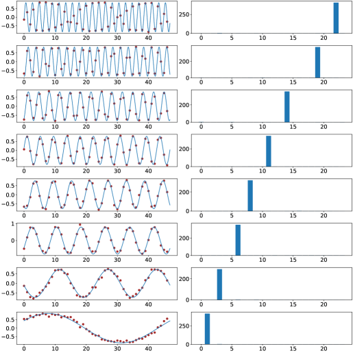
Figure 1: Cosine shape of the trained embeddings (hidden layer weights) and corresponding power of Fourier spectrum. The two-layer network with $m=2944$ neurons is trained on $k=4$-sum mod-$p=47$ addition dataset. We even split the whole datasets ($p^{k}=47^{4}$ data points) into the training and test datasets. Every row represents a random neuron from the network. The left figure shows the final trained embeddings, with red dots indicating the true weight values, and the pale blue interpolation is achieved by identifying the function that shares the same Fourier spectrum. The right figure shows their Fourier power spectrum. The results in these figures are consistent with our analysis statements in Lemma 4.2. See Figure 5, 7 in Appendix G.1 for similar results when $k$ is 3 or 5.

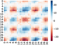
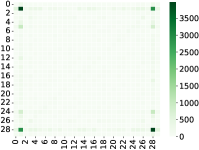
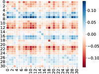
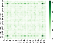
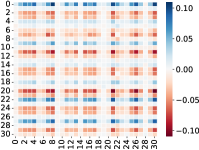
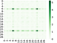
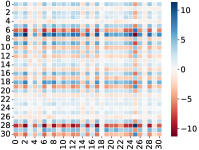
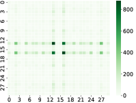
Figure 2: 2-dimension cosine shape of the trained $W^{KQ}$ (attention weights) and their Fourier power spectrum. The one-layer transformer with attention heads $m=160$ is trained on $k=4$-sum mod-$p=31$ addition dataset. We even split the whole datasets ($p^{k}=31^{4}$ data points) into training and test datasets. Every row represents a random attention head from the transformer. The left figure shows the final trained attention weights being an apparent 2-dim cosine shape. The right figure shows their 2-dim Fourier power spectrum. The results in the figures are consistent with Figure 1. See Figure 9 and Figure 10 in Appendix G.2 for similar results when $k$ is 3 or 5.

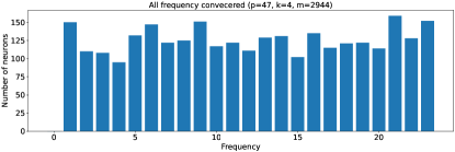
(a)

(b)

(c)

Figure 3: All Fourier spectrum frequencies being covered and the maximum normalized power of the embeddings (hidden layer weights). The one-hidden layer network with $m=2944$ neurons is trained on $k=4$-sum mod-$p=47$ addition dataset. We denote $\widehat{u}[i]$ as the Fourier transform of $u[i]$. Let $\max_{i}|\widehat{u}[i]|^{2}/(\sum|\widehat{u}[j]|^{2})$ be the maximum normalized power. Mapping each neuron to its maximum normalized power frequency, (a) shows the final frequency distribution of the embeddings. Similar to our construction analysis in Lemma 4.3, we have an almost uniform distribution over all frequencies. (b) shows the maximum normalized power of the neural network with random initialization. (c) shows, in frequency space, the embeddings of the final trained network are one-sparse, i.e., maximum normalized power being almost 1 for all neurons. This is consistent with our maximum-margin analysis results in Lemma 4.3. See Figure 6 and Figure 8 in Appendix G.1 for similar results when $k$ is 3 or 5.

4.1 Technique Overview

In this section, we propose techniques overview of the proof for our main result. We use $\mathbf{i}$ to denote $\sqrt{-1}$. Let $f:\mathbb{Z}_{p}\rightarrow\mathbb{C}$. Then, for each frequency $j\in\mathbb{Z}_{p}$, we define $f$ discrete Fourier transform (DFT) as

$$\widehat{f}(j):=\sum_{\zeta\in\mathbb{Z}_{p}}f(\zeta)\exp(-2\pi\mathbf{i}\cdot j\zeta/p).$$

Let ${\cal B}$ denote the ball that $\|w\|^{2}+\|u_{1}\|^{2}+\dots+\|u_{k}\|^{2}\leq 1$. Let $\Omega_{q}^{{}^{\prime}*}$ be defined as Definition C.6. We first show how we get the single neuron class-weighted maximum-margin solution set $\Omega^{\prime*}_{q}$.

Lemma 4.2 (Informal version of Lemma C.8).

If for any $\zeta\in\{1,\ldots,\frac{p-1}{2}\}$, there exists a scaling constant $\beta\in\mathbb{R}$,

$$u_{1}(a_{1}) =\beta\cdot\cos(\theta_{u_{1}}^{*}+2\pi\zeta a_{1}/p)$$

$$u_{2}(a_{2}) =\beta\cdot\cos(\theta_{u_{2}}^{*}+2\pi\zeta a_{2}/p)$$

$$\dots$$

$$u_{k}(a_{k}) =\beta\cdot\cos(\theta_{u_{k}}^{*}+2\pi\zeta a_{k}/p)$$

$$w(c) =\beta\cdot\cos(\theta_{w}^{*}+2\pi\zeta c/p)$$

where $\theta_{u_{1}}^{*},\dots,\theta_{u_{k}}^{*},\theta_{w}^{*}\in\mathbb{R}$ are some phase offsets satisfying $\theta_{u_{1}}^{*}+\dots+\theta_{u_{k}}^{*}=\theta_{w}^{*}$.

Then, we have the following

$$\Omega_{q}^{\prime*}= \{(u_{1},\dots,u_{k},w)\},$$

and

$$\gamma^{*}=\frac{2(k!)}{(2k+2)^{(k+1)/2}(p-1)p^{(k-1)/2}}.$$

Proof sketch of Lemma 4.2.

The proof establishes the maximum-margin solution’s sparsity in the Fourier domain through several key steps. Initially, by Lemma C.7, focus is directed to maximizing Eq. (C.4).

For odd $p$, Eq. (C.4) can be reformulated with magnitudes and phases of $\widehat{u}_{i}$ and $\widehat{w}$ (discrete Fourie transform of $u_{i}$ and $w$), leading to an equation involving cosine of their phase differences. Plancherel’s theorem is then employed to translate the norm constraint to the Fourier domain. This allows for the optimization of the cosine term in the sum, effectively reducing the problem to maximizing the product of magnitudes of $\widehat{u}_{i}$ and $\widehat{w}$ (Eq. (23)).

By applying the inequality of arithmetic and geometric means we have an upper bound for the optimization problem. To achieve the upper bound, equal magnitudes are required for all $\widehat{u}_{i}$ and $\widehat{w}$ at a single frequency, leading to Eq. (27). The neurons are finally expressed in the time domain, demonstrating that they assume a specific cosine form with phase offsets satisfying certain conditions. ∎

See formal proof in Appendix C.3.

Next, we show the number of neurons required to solve the problem and the property of these neurons. We demonstrate how to use these neurons to construct the network $\theta^{*}$.

Lemma 4.3 (Informal version of Lemma D.3).

Let $\cos_{\zeta}(x)$ denote $\cos(2\pi\zeta x/p)$. Then, we have the maximum $L_{2,k+1}$-margin solution $\theta^{*}$ will consist of $2^{2k-1}\cdot{p-1\over 2}$ neurons $\theta^{*}_{i}\in\Omega_{q}^{{}^{\prime}*}$ to simulate $\frac{p-1}{2}$ type of cosine computation, each cosine computation is uniquely determined a $\zeta\in\{1,\ldots,\frac{p-1}{2}\}$. In particular, for each $\zeta$ the cosine computation is $\cos_{\zeta}(a_{1}+\dots+a_{k}-c),\forall a_{1},\dots,a_{k},c\in\mathbb{Z}_{p}$.

Proof sketch of Lemma 4.3.

Our goal is to show that $2^{2k-1}\cdot{p-1\over 2}$ neurons $\theta_{i}^{*}\in\Omega_{q}^{{}^{\prime}*}$ are able to simulate $\frac{p-1}{2}$ type of $\cos$ computation.

We first observe that when the $\cos$ of a sum, $\cos(a_{1}+a_{2})$, is expanded, we will remove one $\cos$ product and we will add zero or two $\sin$ products. On the other hand, expanding the sine of a sum, $\sin(a_{1}+a_{2})$, we may remove one $\sin$ product and we will add one $\sin$ product as well.

The second observation is about the sign of the terms resulting from these expansions. It notes that a negative sign $-1$ appears in a term only when a $\cos$ is split, and adding two sine products. Therefore, if the number of sine products in a term is divisible by $4$ with a remainder of $2$ (i.e., $\%4=2$), the term will have a negative sign. In all other cases, the term will have a positive sign.

By using these two observations, we have the following expansion function of $\cos_{\zeta}(x)$, which denotes $\cos(2\pi\zeta x/p)$.

$$\cos_{\zeta}(\sum_{i=1}^{k}a_{i})= ~{}\sum_{b\in\{0,1\}^{k}}\prod_{i=1}^{k}\cos^{1-b_{i}}(a_{i})\cdot\sin^{b_{i}}(a_{i})$$

$$\cdot{\bf 1}[\sum_{i=1}^{k}b_{i}\%2=0]\cdot(-1)^{{\bf 1}[\sum_{i=1}^{k}b_{i}\%4=2]}.$$

Note that we have $2^{k}$ terms in the above equation. By using the following fact in Lemma D.1,

$$2^{k}\cdot k!\cdot\prod_{i=1}^{k}a_{i}=\sum_{c\in\{-1,+1\}^{k}}(-1)^{(k-\sum_{i=1}^{k}c_{i})/2}(\sum_{j=1}^{k}c_{j}a_{j})^{k},$$

each term can be constructed by $2^{k-1}$ neurons. Therefore, we need $2^{k-1}2^{k}$ total neurons. To simulate $\frac{p-1}{2}$ type of simulation, we need $2^{2k-1}\frac{p-1}{2}$ neurons.

Then, using the Lemma B.1, we construct the network $\theta^{*}$. Finally, by using the Lemma B.2 from [55], we know that it is the maximum-margin solution. ∎

See formal proof in Appendix D.3. Now, we are ready to prove our main results.

Proof sketch of Theorem 4.1.

By Lemma 4.2, we get $\gamma^{*}$ and the single-neuron class-weighted maximum-margin solution set $\Omega_{q}^{{}^{\prime}*}$. By satisfying Condition 3.10, we know it is used in the maximum-margin solution.

By Lemma 4.3, we can construct the network $\theta^{*}$ that uses neurons in $\Omega_{q}^{{}^{\prime}*}$. By Lemma B.2, we know that it is the maximum-margin solution. Finally, by Lemma E.2, we know that all frequencies are covered. ∎

See formal proof in Appendix F.2.

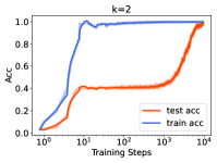
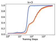
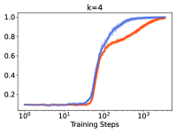
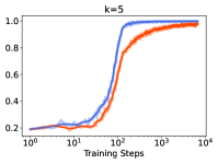
Figure 4: Grokking (models abruptly transition from bad generalization to perfect generalization after a large number of training steps) under learning modular addition involving $k=2,3,4,5$ inputs. We train two-layer transformers with $m=160$ attention heads on $k=2,3,4,5$-sum mod-$p=97,31,11,5$ addition dataset with $50$% of the data in the training set under AdamW [46] optimizer 1e-3 learning rate and 1e-4 weight decay. We use different $p$ to guarantee the dataset sizes are roughly equal to each other. The blue curves show training accuracy and the red ones show validation accuracy. There is a grokking phenomenon in all figures. However, as $k$ increases, the grokking phenomenon becomes weak. It implies that when the ground-truth function class becomes “complicated”, the transformers need to train more steps to overfit the training datasets and the generalization tends to be better.

5 Experiments

In Section 5.1, we conduct simulation experiments to verify our analysis for $k=3,4,5$. In Section 5.2, we show that the one-layer transformer learns 2-dimensional cosine functions in their attention weights. In Section 5.3, we show the grokking phenomenon under different $k$.

5.1 One-hidden Layer Neural Network

We conduct simulation experiments to verify our analysis. In Figure 1 and Figure 3, we use SGD to train a two-layer network with $m=2944=2^{2k-2}\cdot(p-1)$ neurons, i.e., Eq. (2), on $k=4$-sum mod-$p=47$ addition dataset, i.e., Eq. (1). Figure 1 shows that the networks trained with SGD have single-frequency hidden neurons, which support our analysis in Lemma 4.2. Furthermore, Figure 3 demonstrates that the network will learn all frequencies in the Fourier spectrum which is consistent with our analysis in Lemma 4.3. Together, they verify our main results in Theorem 4.1 and show that the network trained by SGD prefers to learn Fourier-based circuits. There are more similar results when $k$ is 3 or 5 in Appendix G.1.

5.2 One-layer Transformer

We find similar results in the one-layer transformer. Recall that the $m$-heads attention layer can be written as

$$W^{P}\begin{pmatrix}W_{1}^{V\top}E\cdot\operatorname{softmax}\left({E^{\top}W_{1}^{K}W_{1}^{Q\top}E}\right)\\ \dots\\ W_{m}^{V\top}E\cdot\operatorname{softmax}\left({E^{\top}W_{m}^{K}W_{m}^{Q\top}E}\right)\end{pmatrix},$$ (7)

where $E$ is input embedding and $W^{P},W^{V},W^{K},W^{Q}$ are projection, value, key and query matrix. We denote $W^{K}W^{Q\top}$ as $W^{KQ}$ and call it attention matrix.

In Figure 2 , we train a one-layer transformer with $m=160$ heads attention, i.e., Eq. (7), on $k=4$-sum mod-$p=31$ addition dataset, i.e., Eq. (1). Figure 2 shows that the SGD trained one-layer transformer learns 2-dim cosine shape attention matrices, which is similar to the one-hidden layer neural networks in Figure 1. This means that the attention layer has a learning mechanism similar to neural networks in the modular arithmetic task. It prefers to learn (2-dim) Fourier-based circuits when trained by SGD. There are more similar results when $k$ is 3 or 5 in Appendix G.2.

5.3 Grokking under Different $k$

Following the experiments’ protocol in [66], we show there is the grokking phenomenon under different $k$. We train two-layer transformers with $m=160$ attention heads on $k=2,3,4,5$-sum mod-$p=97,31,11,5$ addition dataset with 50% of the data in the training. We use different $p$ to guarantee the dataset sizes are roughly equal to each other. As $k$ increases, the grokking phenomenon becomes weak. It implies that when the ground-truth function class becomes “complicated”, the transformers need to train more steps to fit the training datasets and the generalization tends to be better. This is consistent with our analysis. In Theorem 4.1, we show that we need $2^{2k-2}\cdot(p-1)$ neurons to get maximum-margin solution, and we can check this value is $2^{2}\cdot(97-1)=384,2^{4}\cdot(31-1)=480,2^{6}\cdot(11-1)=640,2^{8}\cdot(5-1)=1024$ for $k=2,3,4,5$. It means that, when $k$ becomes larger, although the whole input space size is roughly unchanged, we need more neurons to fit the optimal solution as the function class becomes more “complicated”. Thus, with increasing $k$, if we train the same size of models under these settings, the models will slightly transfer from overfitting to underfitting, so the grokking phenomenon becomes weak.

6 Discussion

Connection to Parity and SQ Hardness.

If we let $p=2$, then $(a_{1}+\dots+a_{k})\bmod p$ will degenerate to parity function, i.e., $b_{1},\dots,b_{k}\in\{\pm 1\}$ and determining $\prod_{i=1}^{k}b_{i}$. Parity functions serve as a fundamental set of learning challenges in computational learning theory, often used to demonstrate computational obstacles [76]. In particular, $(n,k)$-sparse parity problem is notorious hard to learn, i.e., Statistical Query (SQ) hardness [6]. [21] showed that one-hidden layer networks need an $\Omega(\exp(k))$ number of neurons or an $\Omega(\exp(k))$ number of training steps to successfully learn it by SGD. In our work, we are studying Eq. (2), which is a more general function than parity and indeed is a learning hardness. Our Theorem 4.1 states that we need $\Omega(\exp(k))$ number of neurons to represent the maximum-margin solution, which well aligns with existing works. Our experiential results in Section 5.1 are also consistent. Hence, our modular addition involving $k$ inputs function class is a good data model to analyze and test the model learning ability, i.e., approximation power, optimization, and generalization.

High Order Correlation Attention.

[73, 1, 2] state that, when $k=3$, $a_{1}+a_{2}+a_{3}\bmod p$ is hard to be captured by traditional attention. Thus, they introduce high-order attention to capture high-order correlation from the input sequence. However, in Section 5.2, we show that one-layer transformers have a strong learning ability and can successfully learn modular arithmetic tasks even when $k=5$. This implies that the traditional attention may be more powerful than we expect. We conjecture that the layer norm and residual connection contribute as they are ignored by most transformer learning theoretical analysis work [40, 54, 50, 87].

Grokking, Benign Overfitting, and Implicit Bias.

Recently, [94] connects the grokking phenomenon to benign overfitting [7, 11, 84, 24, 26]. It shows how the network undergoes a grokking period from catastrophic to benign overfitting. [47] uses implicit bias [72, 28, 41, 79, 59, 10, 51, 38, 92, 70, 74, 93] to explain grokking, where grokking happens if the early phase bias implies an overfitting solution while late phase bias implies a generalizable solution. The intuition from the benign overfitting and the implicit bias well align with our observation in Section 5.3. It is interesting and valuable to rigorously analyze the grokking or emergent ability under different function class complexities, e.g., Eq (1). We leave this challenge problem as a future work.

7 Conclusion

We study neural networks and transformers learning on $(a_{1}+\dots+a_{k})\bmod p$. We theoretically show that networks prefer to learn Fourier circuits. Our experiments on neural networks and transformers support our analysis. Finally, we study the grokking phenomenon under this new data setting.

Appendix A Notations and Definitions

We use $\mathbf{i}$ to denote $\sqrt{-1}$. Let $z=a+\mathbf{i}b$ denote a complex number where $a$ and $b$ are real numbers. Then we have $\overline{z}=a-\mathbf{i}b$ and $|z|:=\sqrt{a^{2}+b^{2}}$.

For any positive integer $n$, we use $[n]$ to denote set $\{1,2,\cdots,n\}$. We use $\operatorname*{{\mathbb{E}}}[]$ to denote expectation. We use $\Pr[]$ to denote probability. We use $z^{\top}$ to denote the transpose of a vector $z$.

Considering a vector $z$, we denote the $\ell_{2}$ norm as $\|z\|_{2}:=(\sum_{i=1}^{n}z_{i}^{2})^{1/2}$. We denote the $\ell_{1}$ norm as $\|z\|_{1}:=\sum_{i=1}^{n}|z_{i}|$. The number of non-zero entries in vector $z$ is defined as $\|z\|_{0}$. $\|z\|_{\infty}$ is defined as $\max_{i\in[n]}|z_{i}|$.

We denote $\mathbb{Z}_{p}$ as the modular group on $p$ integers, e.g., $\mathbb{Z}_{p}=[p]$, where $p>2$ is a given prime number. We denote $\mathcal{X}:=\mathbb{Z}_{p}^{k}$ as the input space and $\mathcal{Y}:=\mathbb{Z}_{p}$ as the output space. We denote $D_{p}:=\{((a_{1},\dots,a_{k}),\sum_{i\in[k]}a_{i}):a_{1},\dots,a_{k}\in\mathbb{Z}_{p}\}$ as the modular dataset.

Suppose we have a $L_{2,k+1}$ (matrix) norm $\|\cdot\|_{2,k+1}$ (Definition 3.3) and a class of parameterized functions $\{f(\theta,\cdot)\mid\theta\in\mathbb{R}^{U}\}$, where $f:\mathbb{R}^{U}\times\mathcal{X}\rightarrow\mathbb{R}^{\mathcal{Y}}$ and a matrix set $\Theta:=\{\|\theta\|_{2,k+1}\leq 1\}$. We consider single-hidden layer neural networks with polynomial activation functions and without biases. With parameters $\theta\in\Theta$, we denote $f(\theta,x)$ as the network’s output for an input $x$. For one-hidden layer networks, we denote $f$ as:

$$f(\theta,x):=\sum_{i=1}^{m}\phi(\theta_{i},x),$$

where $\theta:=\{\theta_{1},\ldots,\theta_{m}\}$. Here, we denote $\phi$ as one neuron and $\theta_{i}\in\Omega$ are the corresponding weights in that neuron, where $\Omega$ is a vector set. Let $\Omega^{\prime}$ be a subset of $\Omega$. For every $i\in[m]$, when either there exists $\alpha_{i}>0$ such that $\alpha_{i}\theta_{i}\in\Omega^{\prime}$ or $\theta_{i}=0$, then we say the parameter set $\theta=\{\theta_{1},\ldots,\theta_{m}\}$ has directional support on $\Omega^{\prime}$. A single neuron is represented as:

$$\phi(\{u_{1},\dots,u_{k},w\},x_{1},\dots,x_{k}):=~{}(u_{1}^{\top}x_{1}+\dots+u_{k}^{\top}x_{k})^{k}w,$$

where $u_{1},\dots,u_{k},w\in\mathbb{R}^{p}$ are the neuron’s weights, and $x_{1},\dots,x_{k}\in\mathbb{R}^{p}$ are the network inputs. Inputs $x_{1},\dots,x_{k}$ are one-hot vectors representing group elements. For input elements $(a_{1},\dots,a_{k})$, a neuron simplifies to

$$\phi(\{u_{1},\dots,u_{k},w\},a_{1},\dots,a_{k})=(u_{1}(a_{1})+\dots+u_{k}(a_{k}))^{k}w,$$

with $u_{1}(a_{1})$ being the $a_{1}$-th component of $u_{1}$. The output of the neuron is in $p$-dimension for cross-entropy loss. With $\theta=\{u_{i,1},\dots,u_{i,k},w_{i}\}_{i=1}^{m},$ the network is denoted as:

$$~{}f(\theta,a_{1},\dots,a_{k}):=~{}\sum_{i=1}^{m}\phi(\{u_{i,1},\dots,u_{i,k},w_{i}\},a_{1},\dots.a_{k}).$$

We define our regularized training objective function.

Definition A.1.

Let $l$ be the cross-entropy loss. Our regularized training objective function is

$$\mathcal{L}_{\lambda}(\theta):=\frac{1}{|D_{p}|}\sum_{(x,y)\in D_{p}}l(f(\theta,x),y)+\lambda\|\theta\|_{2,k+1}.$$

Definition A.2.

We define $\Theta^{*}$ as follows

• $\Theta^{*}:=\arg\max_{\theta\in\Theta}h(\theta)$.

Appendix B Tools from Previous Work

Section B.1 states that we can use the single neuron level optimization to get the maximum-margin network. Section B.2 introduces the maximum-margin for multi-class.

B.1 Tools from Previous Work: Implying Single/Combined Neurons

Lemma B.1 (Lemma 5 in page 8 in [55]).

If the following conditions hold

• Given $\Theta:=\{\theta:\|\theta\|_{a,b}\leq 1\}$.

• Given $\Theta_{q}^{\prime*}:=\arg\max_{\theta\in\Theta}\operatorname*{{\mathbb{E}}}_{(x,y)\sim q}[g^{\prime}(\theta,x,y)]$.

• Given $\Omega:=\{\theta_{i}:\|\theta_{i}\|_{a}\leq 1\}$.

• Given $\Omega_{q}^{\prime*}:=\arg\max_{\theta_{i}\in\Omega}\operatorname*{{\mathbb{E}}}_{(x,y)\sim q}[\psi^{\prime}(\theta,x,y)]$.

Then:

• Let $\theta\in\Theta_{q}^{\prime*}$. We have $\theta$ only has directional support on $\Omega_{q}^{\prime*}$.

• Given $\theta_{1}^{*},\ldots,\theta_{m}^{*}\in\Omega_{q}^{\prime*}$, we have for any set of neuron scalars where $\sum_{i=1}^{m}\alpha_{i}^{\nu}=1,\alpha_{i}\geq 0$, the weights $\theta=\{\alpha_{i}\theta_{i}^{*}\}_{i=1}^{m}$ is in $\Theta_{q}^{\prime*}$.

Given $q^{*}$, then we can get the $\theta^{*}$ satisfying

$$\theta^{*}\in\underset{\theta\in\Theta}{\arg\min}\underset{(x,y)\sim q^{*}}{\operatorname*{{\mathbb{E}}}}[g^{\prime}(\theta,x,y)].$$ (8)

B.2 Tools from Previous Work: Maximum Margin for Multi-Class

Lemma B.2 (Lemma 6 in page 8 in [55]).

If the following conditions hold

• Given $\Theta=\{\theta:\|\theta\|_{a,b}\leq 1\}$ and $\Theta_{q}^{\prime*}=\arg\max_{\theta\in\Theta}\operatorname*{{\mathbb{E}}}_{(x,y)\sim q}[g^{\prime}(\theta,x,y)]$.

• Given $\Omega=\{\theta_{i}:\|\theta_{i}\|_{a}\leq 1\}$ and $\Omega_{q}^{\prime*}=\arg\max_{\theta_{i}\in\Omega}\operatorname*{{\mathbb{E}}}_{(x,y)\sim q}[\psi^{\prime}(\theta,x,y)]$.

• Suppose that $\exists\{\theta^{*},q^{*}\}$ such that Equations (4) and (8), and 3.10 holds.

Then, we can show:

• $\theta^{*}\in\arg\max_{\theta\in\Theta}g(\theta,x,y)$

• $\forall\widehat{\theta}\in\arg\max_{\theta\in\Theta}\min_{(x,y)\in D}g(\theta,x,y)$ the below properties hold:

  - $\widehat{\theta}$ only has directional support on $\Omega_{q^{*}}^{\prime*}$.

  - $\forall(x,y)\in\operatorname{spt}(q^{*}),f(\widehat{\theta},x,y)-\max_{y^{\prime}\in\mathcal{Y}\backslash\{y\}}f(\widehat{\theta},x,y^{\prime})=\gamma^{*}$.

Appendix C Class-weighted Max-margin Solution of Single Neuron

Section C.1 introduces some definitions. Section C.2 shows how we transfer the problem to discrete Fourier space. Section C.3 proposes the weighted margin of the single neuron. Section C.4 shows how we transfer the problem to discrete Fourier space for general $k$ version. Section C.5 provides the solution set for general $k$ version and the maximum weighted margin for a single neuron.

C.1 Definitions

Definition C.1.

When $k=3$, let

$$\eta_{u_{1},u_{2},u_{3},w}(\delta):=\operatorname*{{\mathbb{E}}}_{a_{1},a_{2},a_{3}}[(u_{1}(a_{1})+u_{2}(a_{2})+u_{3}(a_{3}))^{3}w(a_{1}+a_{2}+a_{3}-\delta)].$$

Definition C.2.

When $k=3$, provided the following conditions are met

• We denote ${\cal B}$ as the ball that $\|u_{1}\|^{2}+\|u_{2}\|^{2}+\|u_{3}\|^{2}+\|w\|^{2}\leq 1$.

We define

$$\Omega_{q}^{\prime*}= \underset{u_{1},u_{2},u_{3},w\in{\cal B}}{\arg\max}(\eta_{u_{1},u_{2},u_{3},w}(0)-\operatorname*{{\mathbb{E}}}_{\delta\neq 0}[\eta_{u_{1},u_{2},u_{3},w}(\delta)]).$$

C.2 Transfer to Discrete Fourier Space

The goal of this section is to prove the following Lemma,

Lemma C.3.

When $k=3$, provided the following conditions are met

• We denote ${\cal B}$ as the ball that $\|u_{1}\|^{2}+\|u_{2}\|^{2}+\|u_{3}\|^{2}+\|w\|^{2}\leq 1$.

• We define $\Omega_{q}^{{}^{\prime}*}$ in Definition C.2.

• We adopt the uniform class weighting: $\forall c^{\prime}\neq a_{1}+a_{2}+a_{3},~{}~{}\tau(a_{1},a_{2},a_{3})[c^{\prime}]:=1/(p-1)$.

We have the following

$$\Omega_{q}^{\prime*}= \underset{u_{1},u_{2},u_{3},,w\in{\cal B}}{\arg\max}\frac{6}{(p-1)p^{3}}\sum_{j\neq 0}\widehat{u}_{1}(j)\widehat{u}_{2}(j)\widehat{u}_{3}(j)\widehat{w}(-j).$$

Proof.

We have

$$\eta_{u_{1},u_{2},u_{3},w}(\delta)= ~{}\operatorname*{{\mathbb{E}}}_{a_{1},a_{2},a_{3}}[(u_{1}(a_{1})+u_{2}(a_{2})+u_{3}(a_{3}))^{3}w(a_{1}+a_{2}+a_{3}-\delta)]$$

$$= ~{}\operatorname*{{\mathbb{E}}}_{a_{1},a_{2},a_{3}}[(u_{1}(a_{1})^{3}+3u_{1}(a_{1})^{2}u_{2}(a_{2})+3u_{1}(a_{1})^{2}u_{3}(a_{3})+3u_{1}(a_{1})u_{2}(a_{2})^{2}$$

$$~{}+6u_{1}(a_{1})u_{2}(a_{2})u_{3}(a_{3})+3u_{1}(a_{1})u_{3}(a_{3})^{2}+u_{2}(a_{2})^{3}+3u_{2}(a_{2})^{2}u_{3}(a_{3})$$

$$~{}+3u_{2}(a_{2})u_{3}(a_{3})^{2}+u_{3}(a_{3})^{3})w(a_{1}+a_{2}+a_{3}-\delta)].$$

Recall ${\cal B}$ is defined as Lemma Statement.

The goal is to solve the following mean margin maximization problem:

$$~{}\underset{u_{1},u_{2},u_{3},w\in{\cal B}}{\arg\max}(\eta_{u_{1},u_{2},u_{3},w}(0)-\operatorname*{{\mathbb{E}}}_{\delta\neq 0}[\eta_{u_{1},u_{2},u_{3},w}(\delta)])$$

$$= ~{}\frac{p}{p-1}(\eta_{u_{1},u_{2},u_{3},w}(0)-\operatorname*{{\mathbb{E}}}_{\delta}[\eta_{u_{1},u_{2},u_{3},w}(\delta)]),$$ (9)

where the equation follows $\tau(a_{1},a_{2},a_{3})[c^{\prime}]:=1/(p-1)~{}~{}\forall c^{\prime}\neq a_{1}+a_{2}+a_{3}$ and $1-{1\over p-1}=\frac{p}{p-1}$.

First, note that

$$~{}\operatorname*{{\mathbb{E}}}_{a_{1},a_{2},a_{3}}[u_{1}(a_{1})^{3}w(a_{1}+a_{2}+a_{3}-\delta)]$$

$$= ~{}\operatorname*{{\mathbb{E}}}_{a_{1}}[u_{1}(a_{1})^{3}\operatorname*{{\mathbb{E}}}_{a_{2},a_{3}}[w(a_{1}+a_{2}+a_{3}-\delta)]]$$

$$= ~{}0,$$

where the first step follows from taking out the $u_{1}(a_{1})$ from the expectation for $a_{2},a_{3}$, and the last step is from the definition of $w$.

Similarly for the $u_{2}(a_{2})^{3}$,$u_{3}(a_{3})^{3}$ components of $\eta$, they equal to $0$.

Note that

$$~{}\operatorname*{{\mathbb{E}}}_{a_{1},a_{2},a_{3}}[u_{1}(a_{1})^{2}u_{2}(a_{2})w(a_{1}+a_{2}+a_{3}-\delta)]$$

$$= ~{}\operatorname*{{\mathbb{E}}}_{a_{1}}[u_{1}(a_{1})^{2}\operatorname*{{\mathbb{E}}}_{a_{2}}[u_{2}(a_{2})\operatorname*{{\mathbb{E}}}_{a_{3}}[w(a_{1}+a_{2}+a_{3}-\delta)]]]$$

$$= ~{}0,$$

where the first step follows from simple algebra and the last step comes from the definition of $w$.

Similarly for the $u_{1}(a_{1})^{2}u_{3}(a_{3})$, $u_{2}(a_{2})^{2}u_{1}(a_{1})$, $u_{2}(a_{2})^{2}u_{3}(a_{3})$, $u_{3}(a_{3})^{2}u_{1}(a_{1})$, $u_{3}(a_{3})^{2}u_{2}(a_{2})$ components of $\eta$, they equal to $0$.

Hence, we can rewrite Eq. (C.2) as

$$\underset{u_{1},u_{2},u_{3},w\in{\cal B}}{\arg\max}\frac{6p}{p-1}(\widetilde{\eta}_{u_{1},u_{2},u_{3},w}(0)-\operatorname*{{\mathbb{E}}}_{\delta}[\widetilde{\eta}_{u_{1},u_{2},u_{3},w}(\delta)]),$$

where

$$\widetilde{\eta}_{u_{1},u_{2},u_{3},w}(\delta):=\operatorname*{{\mathbb{E}}}_{a_{1},a_{2},a_{3}}[u_{1}(a_{1})u_{2}(a_{2})u_{3}(a_{3})w(a_{1}+a_{2}+a_{3}-\delta)].$$

Let $\rho:=e^{2\pi\mathbf{i}/p}$, and let $\widehat{u}_{1},\widehat{u}_{2},\widehat{u}_{3},\widehat{w}$ be the DFT of $u_{1},u_{2},u_{3}$, and $w$ respectively:

$$~{}\widetilde{\eta}_{u_{1},u_{2},u_{3},w}(\delta)$$

$$= ~{}\operatorname*{{\mathbb{E}}}_{a_{1},a_{2},a_{3}}[(\frac{1}{p}\sum_{j_{1}=0}^{p-1}\widehat{u}_{1}(j_{1})\rho^{j_{1}a_{1}})(\frac{1}{p}\sum_{j_{2}=0}^{p-1}\widehat{u}_{2}(j_{2})\rho^{j_{2}a_{2}})(\frac{1}{p}\sum_{j_{3}=0}^{p-1}\widehat{u}_{3}(j_{3})\rho^{j_{3}a_{3}})(\frac{1}{p}\sum_{j_{4}=0}^{p-1}\widehat{w}(j_{4})\rho^{j_{4}(a_{1}+a_{2}+a_{3}-\delta)})]$$

$$= ~{}\frac{1}{p^{4}}\sum_{j_{1},j_{2},j_{3},j_{4}}\widehat{u}_{1}(j_{1})\widehat{u}_{2}(j_{2})\widehat{u}_{3}(j_{3})\widehat{w}(j_{4})\rho^{-j_{4}\delta}(\operatorname*{{\mathbb{E}}}_{a_{1}}[\rho^{(j_{1}+j_{4})a_{1}}])(\operatorname*{{\mathbb{E}}}_{a_{2}}[\rho^{(j_{2}+j_{4})a_{2}}])(\operatorname*{{\mathbb{E}}}_{a_{3}}[\rho^{(j_{3}+j_{4})a_{3}}])$$

$$= ~{}\frac{1}{p^{4}}\sum_{j}\widehat{u}_{1}(j)\widehat{u}_{2}(j)\widehat{u}_{3}(j)\widehat{w}(-j)\rho^{j\delta}\quad$$

where the first step follows from $\rho:=e^{2\pi\mathbf{i}/p}$ and $\widehat{u}_{1},\widehat{u}_{2},\widehat{u}_{3},\widehat{w}$ are the discrete Fourier transforms of $u_{1},u_{2},u_{3},w$, the second step comes from simple algebra, the last step is from that only terms where $j_{1}+j_{4}=j_{2}+j_{4}=j_{3}+j_{4}=0$ survive.

Hence, we need to maximize

$$~{}\frac{6p}{p-1}(\widetilde{\eta}_{u_{1},u_{2},u_{3},w}(0)-\operatorname*{{\mathbb{E}}}_{\delta}[\widetilde{\eta}_{u_{1},u_{2},u_{3},w}(\delta)])$$

$$= ~{}\frac{6p}{p-1}(\frac{1}{p^{4}}\sum_{j}\widehat{u}_{1}(j)\widehat{u}_{2}(j)\widehat{u}_{3}(j)\widehat{w}(-j)-\frac{1}{p^{4}}\sum_{j}\widehat{u}_{1}(j)\widehat{u}_{2}(j)\widehat{u}_{3}(j)\widehat{w}(-j)(\operatorname*{{\mathbb{E}}}_{\delta}\rho^{j\delta}))$$

$$= ~{}\frac{6}{(p-1)p^{3}}\sum_{j\neq 0}\widehat{u}_{1}(j)\widehat{u}_{2}(j)\widehat{u}_{3}(j)\widehat{w}(-j).$$

$$= ~{}\frac{6}{(p-1)p^{3}}\sum_{j\in[-(p-1)/2,+(p-1)/2]\backslash 0}\widehat{u}_{1}(j)\widehat{u}_{2}(j)\widehat{u}_{3}(j)\widehat{w}(-j).$$ (10)

where the first step is from $\widetilde{\eta}_{u_{1},u_{2},u_{3},w}(\delta)$ definition, the second step is from $\operatorname*{{\mathbb{E}}}_{\delta}\rho^{j\delta}=0$ when $j\neq 0$, and the last step follows from simple algebra.

∎

C.3 Get Solution Set

Lemma C.4.

When $k=3$, provided the following conditions are met

• We denote ${\cal B}$ as the ball that $\|u_{1}\|^{2}+\|u_{2}\|^{2}+\|u_{3}\|^{2}+\|w\|^{2}\leq 1$.

• We define $\Omega_{q}^{{}^{\prime}*}$ in Definition C.2.

• We adopt the uniform class weighting: $\forall c^{\prime}\neq a_{1}+a_{2}+a_{3},~{}~{}\tau(a_{1},a_{2},a_{3})[c^{\prime}]:=1/(p-1)$.

• For any $\zeta\in\{1,\ldots,\frac{p-1}{2}\}$, there exists a scaling constant $\beta\in\mathbb{R}$ and

  $$u_{1}(a_{1}) =\beta\cdot\cos(\theta_{u_{1}}^{*}+2\pi\zeta a_{1}/p)$$

  $$u_{2}(a_{2}) =\beta\cdot\cos(\theta_{u_{2}}^{*}+2\pi\zeta a_{2}/p)$$

  $$u_{3}(a_{3}) =\beta\cdot\cos(\theta_{u_{3}}^{*}+2\pi\zeta a_{3}/p)$$

  $$w(c) =\beta\cdot\cos(\theta_{w}^{*}+2\pi\zeta c/p)$$

  where $\theta_{u_{1}}^{*},\theta_{u_{2}}^{*},\theta_{u_{3}}^{*},\theta_{w}^{*}\in\mathbb{R}$ are some phase offsets satisfying $\theta_{u_{1}}^{*}+\theta_{u_{2}}^{*}+\theta_{u_{3}}^{*}=\theta_{w}^{*}$.

Then, we have the following

$$\Omega_{q}^{\prime*}= \{(u_{1},u_{2},u_{3},w)\},$$

and

$$\underset{u_{1},u_{2},u_{3},w\in{\cal B}}{\max}(\eta_{u_{1},u_{2},u_{3},w}(0)-\operatorname*{{\mathbb{E}}}_{\delta\neq 0}[\eta_{u_{1},u_{2},u_{3},w}(\delta)])=\frac{3}{16}\cdot\frac{1}{p(p-1)}.$$

Proof.

By Lemma C.3, we only need to maximize Equation (C.2).

Thus, the mass of $\widehat{u}_{1},\widehat{u}_{2},\widehat{u}_{3}$, and $\widehat{w}$ must be concentrated on the same frequencies. For all $j\in\mathbb{Z}_{p}$, we have

$$\widehat{u}_{1}(-j)=\overline{\widehat{u}_{1}(j)},\widehat{u}_{2}(-j)=\overline{\widehat{u}_{2}(j)},\widehat{u}_{3}(-j)=\overline{\widehat{u}_{3}(j)},\widehat{w}(-j)=\overline{\widehat{w}(j)}$$ (11)

as $u_{1},u_{2},u_{3},w$ are real-valued.

For all $j\in\mathbb{Z}_{p}$ and for $u_{1},u_{2},u_{3},w$, we denote $\theta_{u_{1}},\theta_{u_{2}},\theta_{u_{3}},\theta_{w}\in[0,2\pi)^{p}$ as their phase, e.g.:

$$\widehat{u}_{1}(j)=|\widehat{u}_{1}(j)|\exp(\mathbf{i}\theta_{u_{1}}(j)).$$

Consider the odd $p$, Equation (C.2) becomes:

$$\eqref{eq:discrete_fourier_transforms_uvw}= ~{}\frac{6}{(p-1)p^{3}}\sum_{j\in[-(p-1)/2,+(p-1)/2]\backslash 0}\widehat{u}_{1}(j)\widehat{u}_{2}(j)\widehat{u}_{3}(j)\widehat{w}(-j)$$

$$= ~{}\frac{6}{(p-1)p^{3}}\sum_{j=1}^{(p-1)/2}(\widehat{u}_{1}(j)\widehat{u}_{2}(j)\widehat{u}_{3}(j)\overline{\widehat{w}(j)}+\overline{\widehat{u}_{1}(j)\widehat{u}_{2}(j)\widehat{u}_{3}(j)}\widehat{w}(j))$$

$$= ~{}\frac{6}{(p-1)p^{3}}\sum_{j=1}^{(p-1)/2}|\widehat{u}_{1}(j)||\widehat{u}_{2}(j)||\widehat{u}_{3}(j)||\widehat{w}(j)|\cdot$$

$$~{}\big{(}\exp(\mathbf{i}(\theta_{u_{1}}(j)+\theta_{u_{2}}(j)+\theta_{u_{3}}(j)-\theta_{w}(j))+\exp(\mathbf{i}(-\theta_{u_{1}}(j)-\theta_{u_{2}}(j)-\theta_{u_{3}}(j)+\theta_{w}(j))\big{)}$$

$$= ~{}\frac{12}{(p-1)p^{3}}\sum_{j=1}^{(p-1)/2}|\widehat{u}_{1}(j)||\widehat{u}_{2}(j)||\widehat{u}_{3}(j)||\widehat{w}(j)|\cos(\theta_{u_{1}}(j)+\theta_{u_{2}}(j)+\theta_{u_{3}}(j)-\theta_{w}(j)).$$

where the first step comes from definition (C.2), the second step follows from Eq. (11), the third step comes from $\widehat{u}_{1}(-j)=\overline{\widehat{u}_{1}(j)}$ and $\widehat{u}_{1}(j)=|\widehat{u}_{1}(j)|\exp(\mathbf{i}\theta_{u_{1}}(j))$, the last step follow from Euler’s formula.

Thus, we need to optimize:

$$\max_{u_{1},u_{2},u_{3},w\in{\cal B}}\frac{12}{(p-1)p^{3}}\sum_{j=1}^{(p-1)/2}|\widehat{u}_{1}(j)||\widehat{u}_{2}(j)||\widehat{u}_{3}(j)||\widehat{w}(j)|\cos(\theta_{u_{1}}(j)+\theta_{u_{2}}(j)+\theta_{u_{3}}(j)-\theta_{w}(j)).$$ (12)

The norm constraint $\|u_{1}\|^{2}+\|u_{2}\|^{2}+\|u_{3}\|^{2}+\|w\|^{2}\leq 1$ is equivalent to

$$\|\widehat{u}_{1}\|^{2}+\|\widehat{u}_{2}\|^{2}+\|\widehat{u}_{3}\|^{2}+\|\widehat{w}\|^{2}\leq p$$

by using Plancherel’s theorem. Thus, we need to select them in such a way that

$$\theta_{u_{1}}(j)+\theta_{u_{2}}(j)+\theta_{u_{3}}(j)=\theta_{w}(j),$$

ensuring that, for each $j$, the expression $\cos(\theta_{u_{1}}(j)+\theta_{u_{2}}(j)+\theta_{u_{3}}(j)-\theta_{w}(j))=1$ is maximized, except in cases where the scalar of the $j$-th term is $0$.

This further simplifies the problem to:

$$\max_{|\widehat{u}_{1}|,|\widehat{u}_{2}|,|\widehat{u}_{3}|,|\widehat{w}|:\|\widehat{u}_{1}\|^{2}+\|\widehat{u}_{2}\|^{2}+\|\widehat{u}_{3}\|^{2}+\|\widehat{w}\|^{2}\leq p}\frac{12}{(p-1)p^{3}}\sum_{j=1}^{(p-1)/2}|\widehat{u}_{1}(j)||\widehat{u}_{2}(j)||\widehat{u}_{3}(j)||\widehat{w}(j)|.$$ (13)

Then, we have

$$|\widehat{u}_{1}(j)||\widehat{u}_{2}(j)||\widehat{u}_{3}(j)||\widehat{w}(j)|\leq(\frac{1}{4}\cdot(|\widehat{u}_{1}(j)|^{2}+|\widehat{u}_{2}(j)|^{2}+|\widehat{u}_{3}(j)|^{2}+|\widehat{w}(j)|^{2}))^{2}.$$ (14)

where the first step is from inequality of quadratic and geometric means.

We define $z:\{1,\ldots,\frac{p-1}{2}\}\rightarrow\mathbb{R}$ as

$$z(j):=|\widehat{u}_{1}(j)|^{2}+|\widehat{u}_{2}(j)|^{2}+|\widehat{u}_{3}(j)|^{2}+|\widehat{w}(j)|^{2}.$$

We need to have $\widehat{u}_{1}(0)=\widehat{u}_{2}(0)=\widehat{u}_{3}(0)=\widehat{w}(0)=0$. Then, the upper-bound of Eq. (13) is given by

$$~{}\frac{12}{(p-1)p^{3}}\cdot\max_{\|z\|_{1}\leq\frac{p}{2}}\sum_{j=1}^{(p-1)/2}(\frac{z(j)}{4})^{2}$$

$$= ~{}\frac{3}{4(p-1)p^{3}}\cdot\max_{\|z\|_{1}\leq\frac{p}{2}}\sum_{j=1}^{(p-1)/2}z(j)^{2}$$

$$= ~{}\frac{3}{4(p-1)p^{3}}\cdot\max_{\|z\|_{1}\leq\frac{p}{2}}\|z\|_{2}^{2}$$

$$\leq ~{}\frac{3}{4(p-1)p^{3}}\cdot\frac{p^{2}}{4}$$

$$= ~{}\frac{3}{16}\cdot\frac{1}{p(p-1)},$$

where the first step follows from simple algebra, the second step comes from the definition of $L_{2}$ norm, the third step follows from $\|z\|_{2}\leq\|z\|_{1}\leq\frac{p}{2}$, the last step comes from simple algebra.

For the inequality of quadratic and geometric means, Eq. (14) becomes equality when $|\widehat{u}_{1}(j)|=|\widehat{u}_{2}(j)|=|\widehat{u}_{3}(j)|=|\widehat{w}(j)|$. To achieve $\|z\|_{2}=\frac{p}{2}$, all the mass must be placed on a single frequency. Hence, for some frequency $\zeta\in\{1,\ldots,\frac{p-1}{2}\}$, to achieve the upper bound, we have:

$$|\widehat{u}_{1}(j)|=|\widehat{u}_{2}(j)|=|\widehat{u}_{3}(j)|=|\widehat{w}(j)|=\Big{\{}\begin{array}[]{ll}\sqrt{p/8}&\text{ if }j=\pm\zeta\\ 0&\text{ otherwise }\end{array},$$ (17)

In this case, Eq. (13) matches the upper bound.

$$\frac{12}{(p-1)p^{3}}\cdot(\frac{p}{8})^{2}=\frac{3}{16}\cdot\frac{1}{p(p-1)},$$

where the first step is by simple algebra. Hence, the maximum-margin is $\frac{3}{16}\cdot\frac{1}{p(p-1)}$.

Let $\theta_{u_{1}}^{*}:=\theta_{u_{1}}(\zeta)$. Combining all the results, up to scaling, it is established that all neurons which maximize the expected class-weighted margin conform to the form:

$$u_{1}(a_{1})= ~{}\frac{1}{p}\sum_{j=0}^{p-1}\widehat{u}_{1}(j)\rho^{ja_{1}}$$

$$= ~{}\frac{1}{p}\cdot(\widehat{u}_{1}(\zeta)\rho^{\zeta a_{1}}+\widehat{u}_{1}(-\zeta)\rho^{-\zeta a_{1}})$$

$$= ~{}\frac{1}{p}\cdot(\sqrt{\frac{p}{8}}\exp(\mathbf{i}\theta_{u_{1}}^{*})\rho^{\zeta a_{1}}+\sqrt{\frac{p}{8}}\exp(-\mathbf{i}\theta_{u_{1}}^{*})\rho^{-\zeta a_{1}})$$

$$= ~{}\sqrt{\frac{1}{2p}}\cos(\theta_{u_{1}}^{*}+2\pi\zeta a_{1}/p),$$

where the first step comes from the definition of $u_{1}(a)$, the second step and third step follow from Eq. (17), the last step follows from Euler’s formula.

Similarly,

$$u_{2}(a_{2})= ~{}\sqrt{\frac{1}{2p}}\cos(\theta_{u_{2}}^{*}+2\pi\zeta a_{2}/p)$$

$$u_{3}(a_{3})= ~{}\sqrt{\frac{1}{2p}}\cos(\theta_{u_{3}}^{*}+2\pi\zeta a_{3}/p)$$

$$w(c)= ~{}\sqrt{\frac{1}{2p}}\cos(\theta_{w}^{*}+2\pi\zeta c/p),$$

for some phase offsets $\theta_{u_{1}}^{*},\theta_{u_{2}}^{*},\theta_{u_{3}}^{*},\theta_{w}^{*}\in\mathbb{R}$ satisfying $\theta_{u_{1}}^{*}+\theta_{u_{2}}^{*}+\theta_{u_{3}}^{*}=\theta_{w}^{*}$ and some $\zeta\in\mathbb{Z}_{p}\backslash\{0\}$, where $u_{1},u_{2},u_{3}$, and $w$ shares the same $\zeta$.

∎

C.4 Transfer to Discrete Fourier Space for General $k$ Version

Definition C.5.

Let

$$\eta_{u_{1},\dots,u_{k},w}(\delta):=\operatorname*{{\mathbb{E}}}_{a_{1},\dots,a_{k}}[(u_{1}(a_{1})+\dots+u_{k}(a_{k}))^{k}w(a_{1}+\dots+a_{k}-\delta)].$$

Definition C.6.

Provided the following conditions are met

• We denote ${\cal B}$ as the ball that $\|u_{1}\|^{2}+\dots+\|u_{k}\|^{2}+\|w\|^{2}\leq 1$.

We define

$$\Omega_{q}^{\prime*}= \underset{u_{1},\dots,u_{k},w\in{\cal B}}{\arg\max}(\eta_{u_{1},\dots,u_{k},w}(0)-\operatorname*{{\mathbb{E}}}_{\delta\neq 0}[\eta_{u_{1},\dots,u_{k},w}(\delta)]).$$

The goal of this section is to prove the following Lemma,

Lemma C.7.

Provided the following conditions are met

• Let ${\cal B}$ denote the ball that $\|u_{1}\|^{2}+\dots+\|u_{k}\|^{2}+\|w\|^{2}\leq 1$.

• We define $\Omega_{q}^{{}^{\prime}*}$ in Definition C.6.

• We adopt the uniform class weighting: $\forall c^{\prime}\neq a_{1}+\dots+a_{k},~{}~{}\tau(a_{1},\dots,a_{k})[c^{\prime}]:=1/(p-1)$.

We have the following

$$\Omega_{q}^{\prime*}= \underset{u_{1},\dots,u_{k},w\in{\cal B}}{\arg\max}\frac{k!}{(p-1)p^{k}}\sum_{j\neq 0}\widehat{w}(-j)\prod_{i=1}^{k}\widehat{u}_{i}(j).$$

Proof.

We have

$$\eta_{u_{1},\dots,u_{k},w}(\delta)= ~{}\operatorname*{{\mathbb{E}}}_{a_{1},\dots,a_{k}}[(u_{1}(a_{1})+\dots+u_{k}(a_{k}))^{k}w(a_{1}+\dots+a_{k}-\delta)].$$

The goal is to solve the following mean margin maximization problem:

$$~{}\underset{u_{1},\dots,u_{k},w\in{\cal B}}{\arg\max}(\eta_{u_{1},\dots,u_{k},w}(0)-\operatorname*{{\mathbb{E}}}_{\delta\neq 0}[\eta_{u_{1},\dots,u_{k},w}(\delta)])$$

$$= ~{}\frac{p}{p-1}(\eta_{u_{1},\dots,u_{k},w}(0)-\operatorname*{{\mathbb{E}}}_{\delta}[\eta_{u_{1},\dots,u_{k},w}(\delta)]),$$ (18)

where the equation follows $\tau(a_{1},\dots,a_{k})[c^{\prime}]:=1/(p-1)~{}~{}\forall c^{\prime}\neq a_{1}+\dots+a_{k}$ and $1-{1\over p-1}=\frac{p}{p-1}$.

We note that all terms are zero rather than $w(\cdot)\cdot\prod_{i=1}^{k}u_{i}(a_{i})$.

Hence, we can rewrite Eq. (C.4) as

$$\underset{u_{1},\dots,u_{k},w\in{\cal B}}{\arg\max}\frac{k!p}{p-1}(\widetilde{\eta}_{u_{1},\dots,u_{k},w}(0)-\operatorname*{{\mathbb{E}}}_{\delta}[\widetilde{\eta}_{u_{1},\dots,u_{k},w}(\delta)]),$$

where

$$\widetilde{\eta}_{u_{1},\dots,u_{k},w}(\delta):=\operatorname*{{\mathbb{E}}}_{a_{1},\dots,a_{k}}[w(a_{1}+\dots+a_{k}-\delta)\prod_{i=1}^{k}u_{i}(a_{i})].$$

Let $\rho:=e^{2\pi\mathbf{i}/p}$, and $\widehat{u}_{1},\dots,\widehat{u}_{k},\widehat{w}$ denote the discrete Fourier transforms of $u_{1},\dots,u_{k}$, and $w$ respectively. We have

$$~{}\widetilde{\eta}_{u_{1},\dots,u_{k},w}(\delta)=\frac{1}{p^{k+1}}\sum_{j=0}^{p-1}\widehat{w}(-j)\rho^{j\delta}\prod_{i=1}^{k}\widehat{u}_{i}(j)$$

which comes from $\rho:=e^{2\pi\mathbf{i}/p}$ and $\widehat{u}_{1},\dots,\widehat{u}_{k},\widehat{w}$ are the discrete Fourier transforms of $u_{1},\dots,u_{k},w$.

Hence, we need to maximize

$$~{}\frac{k!p}{p-1}(\widetilde{\eta}_{u_{1},\dots,u_{k},w}(0)-\operatorname*{{\mathbb{E}}}_{\delta}[\widetilde{\eta}_{u_{1},\dots,u_{k},w}(\delta)])$$

$$= ~{}\frac{k!p}{p-1}\cdot\left(\frac{1}{p^{k+1}}\sum_{j=0}^{p-1}\widehat{w}(-j)\prod_{i=1}^{k}\widehat{u}_{i}(j)-\frac{1}{p^{k+1}}\sum_{j=0}^{p-1}\widehat{w}(-j)(\operatorname*{{\mathbb{E}}}_{\delta}[\rho^{j\delta}])\prod_{i=1}^{k}\widehat{u}_{i}(j)\right)$$

$$= ~{}\frac{k!}{(p-1)p^{k}}\sum_{j\neq 0}\widehat{w}(-j)\prod_{i=1}^{k}\widehat{u}_{i}(j).$$

$$= ~{}\frac{k!}{(p-1)p^{k}}\sum_{j\in[-(p-1)/2,+(p-1)/2]\backslash 0}\widehat{w}(-j)\prod_{i=1}^{k}\widehat{u}_{i}(j).$$ (19)

where the first step follows from the definition of $\widetilde{\eta}_{u_{1},\dots,u_{k},w}(\delta)$, the second step follows from $\operatorname*{{\mathbb{E}}}_{\delta}[\rho^{j\delta}]=0$ when $j\neq 0$, the last step is from simple algebra.

∎

C.5 Get Solution Set for General $k$ Version

Lemma C.8 (Formal version of Lemma 4.2).

Provided the following conditions are met

• We denote ${\cal B}$ as the ball that $\|u_{1}\|^{2}+\dots+\|u_{k}\|^{2}+\|w\|^{2}\leq 1$.

• Let $\Omega_{q}^{{}^{\prime}*}$ be defined as Definition C.6.

• We adopt the uniform class weighting: $\forall c^{\prime}\neq a_{1}+\dots+a_{k},~{}~{}\tau(a_{1},\dots,a_{k})[c^{\prime}]:=1/(p-1)$.

• For any $\zeta\in\{1,\ldots,\frac{p-1}{2}\}$, there exists a scaling constant $\beta\in\mathbb{R}$ and

  $$u_{1}(a_{1}) =\beta\cdot\cos(\theta_{u_{1}}^{*}+2\pi\zeta a_{1}/p)$$

  $$u_{2}(a_{2}) =\beta\cdot\cos(\theta_{u_{2}}^{*}+2\pi\zeta a_{2}/p)$$

  $$\dots$$

  $$u_{k}(a_{k}) =\beta\cdot\cos(\theta_{u_{k}}^{*}+2\pi\zeta a_{k}/p)$$

  $$w(c) =\beta\cdot\cos(\theta_{w}^{*}+2\pi\zeta c/p)$$

  where $\theta_{u_{1}}^{*},\dots,\theta_{u_{k}}^{*},\theta_{w}^{*}\in\mathbb{R}$ are some phase offsets satisfying $\theta_{u_{1}}^{*}+\dots+\theta_{u_{k}}^{*}=\theta_{w}^{*}$.

Then, we have the following

$$\Omega_{q}^{\prime*}= \{(u_{1},\dots,u_{k},w)\},$$

and

$$\underset{u_{1},\dots,u_{k},w\in{\cal B}}{\max}(\eta_{u_{1},\dots,u_{k},w}(0)-\operatorname*{{\mathbb{E}}}_{\delta\neq 0}[\eta_{u_{1},\dots,u_{k},w}(\delta)])=\frac{2(k!)}{(2k+2)^{(k+1)/2}(p-1)p^{(k-1)/2}}.$$

Proof.

By Lemma C.7, we only need to maximize Equation (C.4). Thus, the mass of $\widehat{u}_{1},\dots,\widehat{u}_{k}$, and $\widehat{w}$ must be concentrated on the same frequencies. For all $j\in\mathbb{Z}_{p}$, we have

$$\widehat{u}_{i}(-j)=\overline{\widehat{u}_{i}(j)},~{}~{}~{}\widehat{w}(-j)=\overline{\widehat{w}(j)}$$ (20)

as $u_{1},\dots,u_{k},w$ are real-valued. For all $j\in\mathbb{Z}_{p}$ and for $u_{1},u_{2},u_{3},w$, we denote $\theta_{u_{1}},\dots,\theta_{u_{k}},\theta_{w}\in[0,2\pi)^{p}$ as their phase, e.g.:

$$\widehat{u}_{1}(j)=|\widehat{u}_{1}(j)|\exp(\mathbf{i}\theta_{u_{1}}(j)).$$ (21)

Considering odd $p$, Equation (C.4) becomes:

$$\eqref{eq:discrete_fourier_transforms_uvw-k}= ~{}\frac{k!}{(p-1)p^{k}}\sum_{j\in[-(p-1)/2,+(p-1)/2]\backslash 0}\widehat{w}(-j)\prod_{i=1}^{k}\widehat{u}_{i}(j)$$

$$= ~{}\frac{k!}{(p-1)p^{k}}\sum_{j=1}^{(p-1)/2}(\prod_{i=1}^{k}\widehat{u}_{i}(j)\overline{\widehat{w}(j)}+\widehat{w}(j)\prod_{i=1}^{k}\overline{\widehat{u}_{i}(j)})$$

$$= ~{}\frac{2(k!)}{(p-1)p^{k}}\sum_{j=1}^{(p-1)/2}|\widehat{w}(j)|\cos(\sum_{i=1}^{k}\theta_{u_{i}}(j)-\theta_{w}(j))\prod_{i=1}^{k}|\widehat{u}_{i}(j)|.$$

where the first step follows from definition (C.4), the second step comes from Eq. (20), the last step follows from Eq. (21), i.e., Euler’s formula.

Thus, we need to optimize:

$$\max_{u_{1},\dots,u_{k},w\in{\cal B}}\frac{2(k!)}{(p-1)p^{k}}\sum_{j=1}^{(p-1)/2}|\widehat{w}(j)|\cos(\sum_{i=1}^{k}\theta_{u_{i}}(j)-\theta_{w}(j))\prod_{i=1}^{k}|\widehat{u}_{i}(j)|.$$ (22)

We can transfer the norm constraint to

$$\|\widehat{u}_{1}\|^{2}+\dots+\|\widehat{u}_{k}\|^{2}+\|\widehat{w}\|^{2}\leq p$$

by using Plancherel’s theorem.

Therefore, we need to select them in a such way that $\theta_{u_{1}}(j)+\dots+\theta_{u_{k}}(j)=\theta_{w}(j)$, ensuring that, for each $j$, the expression $\cos(\theta_{u_{1}}(j)+\dots+\theta_{u_{k}}(j)-\theta_{w}(j))=1$ is maximized, except in cases where the scalar of the $j$-th term is $0$.

This further simplifies the problem to:

$$\max_{\|\widehat{u}_{1}\|^{2}+\dots+\|\widehat{u}_{k}\|^{2}+\|\widehat{w}\|^{2}\leq p}\frac{2(k!)}{(p-1)p^{k}}\sum_{j=1}^{(p-1)/2}|\widehat{w}(j)|\prod_{i=1}^{k}|\widehat{u}_{i}(j)|.$$ (23)

Then, we have

$$|\widehat{w}(j)|\prod_{i=1}^{k}|\widehat{u}_{i}(j)|\leq(\frac{1}{k+1}\cdot(|\widehat{u}_{1}(j)|^{2}+\dots+|\widehat{u}_{k}(j)|^{2}+|\widehat{w}(j)|^{2}))^{(k+1)/2}.$$ (24)

where the first step follows from inequality of quadratic and geometric means.

We define $z:\{1,\ldots,\frac{p-1}{2}\}\rightarrow\mathbb{R}$, where

$$z(j):=|\widehat{u}_{1}(j)|^{2}+\dots+|\widehat{u}_{k}(j)|^{2}+|\widehat{w}(j)|^{2}.$$

We need to have $\widehat{u}_{1}(0)=\dots=\widehat{u}_{k}(0)=\widehat{w}(0)=0$. Then, the upper-bound of Equation (23) is given by

$$~{}\frac{2(k!)}{(p-1)p^{k}}\cdot\max_{\|z\|_{1}\leq\frac{p}{2}}\sum_{j=1}^{(p-1)/2}(\frac{z(j)}{k+1})^{(k+1)/2}$$

$$= ~{}\frac{2(k!)}{(k+1)^{(k+1)/2}(p-1)p^{k}}\cdot\max_{\|z\|_{1}\leq\frac{p}{2}}\sum_{j=1}^{(p-1)/2}z(j)^{(k+1)/2}$$

$$\leq ~{}\frac{2(k!)}{(k+1)^{(k+1)/2}(p-1)p^{k}}\cdot(p/2)^{(k+1)/2}$$

$$= ~{}\frac{2(k!)}{(2k+2)^{(k+1)/2}(p-1)p^{(k-1)/2}},$$

where the first step follows from simple algebra, the second step comes from the definition of $L_{2}$ norm, the third step follows from $\|z\|_{2}\leq\|z\|_{1}\leq\frac{p}{2}$, the last step follows from simple algebra.

For the inequality of quadratic and geometric means, Eq. (24) becomes equality when $|\widehat{u}_{1}(j)|=\dots=|\widehat{u}_{k}(j)|=|\widehat{w}(j)|$. To achieve $\|z\|_{2}=\frac{p}{2}$, all the mass must be placed on a single frequency. Hence, for some frequency $\zeta\in\{1,\ldots,\frac{p-1}{2}\}$, to achieve the upper bound, we have:

$$|\widehat{u}_{1}(j)|=\dots=|\widehat{u}_{k}(j)|=|\widehat{w}(j)|=\Big{\{}\begin{array}[]{ll}\sqrt{p\over 2(k+1)},&\text{ if }j=\pm\zeta;\\ 0,&\text{ otherwise. }\end{array}$$ (27)

In this case, Equation (23) matches the upper bound. Hence, this is the maximum-margin.

Let $\theta_{u_{1}}^{*}:=\theta_{u_{1}}(\zeta)$. Combining all the results, up to scaling, it is established that all neurons which maximize the expected class-weighted margin conform to the form:

$$u_{1}(a_{1})= ~{}\frac{1}{p}\sum_{j=0}^{p-1}\widehat{u}_{1}(j)\rho^{ja_{1}}$$

$$= ~{}\frac{1}{p}\cdot(\widehat{u}_{1}(\zeta)\rho^{\zeta a_{1}}+\widehat{u}_{1}(-\zeta)\rho^{-\zeta a_{1}})$$

$$= ~{}\frac{1}{p}\cdot(\sqrt{\frac{p}{2(k+1)}}\exp(\mathbf{i}\theta_{u_{1}}^{*})\rho^{\zeta a_{1}}+\sqrt{\frac{p}{2(k+1)}}\exp(-\mathbf{i}\theta_{u_{1}}^{*})\rho^{-\zeta a_{1}})$$

$$= ~{}\sqrt{\frac{2}{(k+1)p}}\cos(\theta_{u_{1}}^{*}+2\pi\zeta a_{1}/p),$$

where the first step comes from the definition of $u_{1}(a)$, the second step and third step follow from Eq. (27), the last step follows from Eq. (21) i.e., Euler’s formula.

We have similar results for other neurons where $\theta_{u_{1}}^{*},\dots,\theta_{u_{k}}^{*},\theta_{w}^{*}\in\mathbb{R}$ satisfying $\theta_{u_{1}}^{*}+\dots+\theta_{u_{k}}^{*}=\theta_{w}^{*}$ and some $\zeta\in\mathbb{Z}_{p}\backslash\{0\}$, where $u_{1},\dots,u_{k}$, and $w$ shares the same $\zeta$.

∎

Appendix D Construct Max Margin Solution

Section D.1 proposed the sum-to-product identities for $k$ inputs. Section D.2 shows how we construct $\theta^{*}$ when $k=3$. Section D.3 gives the constructions for $\theta^{*}$ for general $k$ version.

D.1 Sum-to-product Identities

Lemma D.1 (Sum-to-product Identities).

If the following conditions hold

• Let $a_{1},\dots,a_{k}$ denote any $k$ real numbers

We have

• Part 1.

  $$2^{2}\cdot 2!\cdot a_{1}a_{2} =(a_{1}+a_{2})^{2}-(a_{1}-a_{2})^{2}-(-a_{1}+a_{2})^{2}+(-a_{1}-a_{2})^{2}$$

• Part 2.

  $$2^{3}\cdot 3!\cdot a_{1}a_{2}a_{3} =(a_{1}+a_{2}+a_{3})^{3}-(a_{1}+a_{2}-a_{3})^{3}-(a_{1}-a_{2}+a_{3})^{3}-(-a_{1}+a_{2}+a_{3})^{3}$$

  $$+(a_{1}-a_{2}-a_{3})^{3}+(-a_{1}+a_{2}-a_{3})^{3}+(-a_{1}-a_{2}+a_{3})^{3}-(-a_{1}-a_{2}-a_{3})^{3}$$

• Part 3.

  $$2^{4}\cdot 4!\cdot a_{1}a_{2}a_{3}a_{4}=$$

  $$(a_{1}+a_{2}+a_{3}+a_{4})^{4}$$

  $$-(a_{1}+a_{2}+a_{3}-a_{4})^{4}-(a_{1}+a_{2}-a_{3}+a_{4})^{4}-(a_{1}-a_{2}+a_{3}+a_{4})^{4}-(-a_{1}+a_{2}+a_{3}+a_{4})^{4}$$

  $$+(a_{1}+a_{2}-a_{3}-a_{4})^{4}+(a_{1}-a_{2}+a_{3}-a_{4})^{4}+(a_{1}-a_{2}-a_{3}+a_{4})^{4}$$

  $$+(-a_{1}-a_{2}+a_{3}+a_{4})^{4}+(-a_{1}+a_{2}-a_{3}+a_{4})^{4}+(-a_{1}+a_{2}+a_{3}-a_{4})^{4}$$

  $$-(-a_{1}-a_{2}-a_{3}+a_{4})^{4}-(-a_{1}-a_{2}+a_{3}-a_{4})^{4}-(-a_{1}+a_{2}-a_{3}-a_{4})^{4}-(a_{1}-a_{2}-a_{3}-a_{4})^{4}$$

  $$+(-a_{1}-a_{2}-a_{3}-a_{4})^{4}$$

• Part 4.

  $$2^{k}\cdot k!\cdot\prod_{i=1}^{k}a_{i}=\sum_{c\in\{-1,+1\}^{k}}(-1)^{(k-\sum_{i=1}^{k}c_{i})/2}(\sum_{j=1}^{k}c_{j}a_{j})^{k}.$$

Proof.

Proof of Part 1.

We define $A_{1},A_{2},A_{3},A_{4}$ as follows

$$A_{1}:=~{}(a_{1}+a_{2})^{2},A_{2}:=~{}(a_{1}-a_{2})^{2},A_{3}:=~{}(-a_{1}+a_{2})^{2},A_{4}:=~{}(-a_{1}-a_{2})^{2},$$

For the first term, we have

$$A_{1}= ~{}a_{1}^{2}+a_{2}^{2}+2a_{1}a_{2}.$$

For the second term, we have

$$A_{2}= ~{}a_{1}^{2}+a_{2}^{2}-2a_{1}a_{2}.$$

For the third term, we have

$$A_{3}= ~{}a_{1}^{2}+a_{2}^{2}-2a_{1}a_{2}.$$

For the fourth term, we have

$$A_{4}= ~{}a_{1}^{2}+a_{2}^{2}+2a_{1}a_{2}.$$

Putting things together, we have

$$(a_{1}+a_{2})^{2}-(a_{1}-a_{2})^{2}-(-a_{1}+a_{2})^{2}+(-a_{1}-a_{2})^{2}$$

$$= ~{}A_{1}-A_{2}-A_{3}+A_{4}$$

$$= ~{}8a_{1}a_{2}$$

$$= ~{}2^{3}a_{1}a_{2}$$

Proof of Part 2.

We define $B_{1},B_{2},B_{3},B_{4},B_{5},B_{6},B_{7},B_{8}$ as follows

$$B_{1}:= ~{}(a_{1}+a_{2}+a_{3})^{3},$$

$$B_{2}:= ~{}(a_{1}+a_{2}-a_{3})^{3},$$

$$B_{3}:= ~{}(a_{1}-a_{2}+a_{3})^{3},$$

$$B_{4}:= ~{}(-a_{1}+a_{2}+a_{3})^{3},$$

$$B_{5}:= ~{}(a_{1}-a_{2}-a_{3})^{3},$$

$$B_{6}:= ~{}(-a_{1}+a_{2}-a_{3})^{3},$$

$$B_{7}:= ~{}(-a_{1}-a_{2}+a_{3})^{3},$$

$$B_{8}:= ~{}(-a_{1}-a_{2}-a_{3})^{3},$$

For the first term, we have

$$B_{1}= ~{}a_{1}^{3}+a_{2}^{3}+a_{3}^{3}+3a_{2}a_{3}^{2}+3a_{2}a_{1}^{2}+3a_{1}a_{3}^{2}+3a_{1}a_{2}^{2}+3a_{3}a_{1}^{2}+3a_{3}a_{2}^{2}+6a_{1}a_{2}a_{3}.$$

For the second term, we have

$$B_{2}= ~{}a_{1}^{3}+a_{2}^{3}-a_{3}^{3}+3a_{2}a_{3}^{2}+3a_{2}a_{1}^{2}+3a_{1}a_{3}^{2}+3a_{1}a_{2}^{2}-3a_{3}a_{1}^{2}-3a_{3}a_{2}^{2}-6a_{1}a_{2}a_{3}.$$

For the third term, we have

$$B_{3}= ~{}a_{1}^{3}-a_{2}^{3}+a_{3}^{3}-3a_{2}a_{3}^{2}-3a_{2}a_{1}^{2}+3a_{1}a_{3}^{2}+3a_{1}a_{2}^{2}+3a_{3}a_{1}^{2}+3a_{3}a_{2}^{2}-6a_{1}a_{2}a_{3}.$$

For the fourth term, we have

$$B_{4}= ~{}-a_{1}^{3}+a_{2}^{3}+a_{3}^{3}+3a_{2}a_{3}^{2}+3a_{2}a_{1}^{2}-3a_{1}a_{3}^{2}-3a_{1}a_{2}^{2}+3a_{3}a_{1}^{2}+3a_{3}a_{2}^{2}-6a_{1}a_{2}a_{3}.$$

For the fifth term, we have

$$B_{5}= ~{}a_{1}^{3}-a_{2}^{3}-a_{3}^{3}-3a_{2}a_{3}^{2}-3a_{2}a_{1}^{2}+3a_{1}a_{3}^{2}+3a_{1}a_{2}^{2}-3a_{3}a_{1}^{2}-3a_{3}a_{2}^{2}+6a_{1}a_{2}a_{3}.$$

For the sixth term, we have

$$B_{6}= ~{}-a_{1}^{3}+a_{2}^{3}-a_{3}^{3}+3a_{2}a_{3}^{2}+3a_{2}a_{1}^{2}-3a_{1}a_{3}^{2}-3a_{1}a_{2}^{2}-3a_{3}a_{1}^{2}-3a_{3}a_{2}^{2}+6a_{1}a_{2}a_{3}.$$

For the seventh term, we have

$$B_{7}= ~{}-a_{1}^{3}-a_{2}^{3}+a_{3}^{3}-3a_{2}a_{3}^{2}-3a_{2}a_{1}^{2}-3a_{1}a_{3}^{2}-3a_{1}a_{2}^{2}+3a_{3}a_{1}^{2}+3a_{3}a_{2}^{2}+6a_{1}a_{2}a_{3}.$$

For the eighth term, we have

$$B_{8}= ~{}-a_{1}^{3}-a_{2}^{3}-a_{3}^{3}-3a_{2}a_{3}^{2}-3a_{2}a_{1}^{2}-3a_{1}a_{3}^{2}-3a_{1}a_{2}^{2}-3a_{3}a_{1}^{2}-3a_{3}a_{2}^{2}-6a_{1}a_{2}a_{3}.$$

Putting things together, we have

$$(a_{1}+a_{2}+a_{3})^{3}-(a_{1}+a_{2}-a_{3})^{3}-(a_{1}-a_{2}+a_{3})^{3}-(-a_{1}+a_{2}+a_{3})^{3}$$

$$+(a_{1}-a_{2}-a_{3})^{3}+(-a_{1}+a_{2}-a_{3})^{3}+(-a_{1}-a_{2}+a_{3})^{3}-(-a_{1}-a_{2}-a_{3})^{3}$$

$$= ~{}B_{1}-B_{2}-B_{3}-B_{4}+B_{5}+B_{6}+B_{7}-B_{8}$$

$$= ~{}48a_{1}a_{2}a_{3}$$

$$= ~{}3\cdot 2^{4}a_{1}a_{2}a_{3}$$

Proof of Part 3.

We define $C_{1},C_{2},C_{3},C_{4},C_{5},C_{6},C_{7},C_{8},C_{9},C_{10},C_{11},C_{12},C_{13},C_{14},C_{15},C_{16}$ as follows

$$C_{1}:= ~{}(a_{1}+a_{2}+a_{3}+a_{4})^{4},$$

$$C_{2}:= ~{}(a_{1}+a_{2}+a_{3}-a_{4})^{4},$$

$$C_{3}:= ~{}(a_{1}+a_{2}-a_{3}+a_{4})^{4},$$

$$C_{4}:= ~{}(a_{1}-a_{2}+a_{3}+a_{4})^{4},$$

$$C_{5}:= ~{}(-a_{1}+a_{2}+a_{3}+a_{4})^{4},$$

$$C_{6}:= ~{}(a_{1}+a_{2}-a_{3}-a_{4})^{4},$$

$$C_{7}:= ~{}(a_{1}-a_{2}+a_{3}-a_{4})^{4},$$

$$C_{8}:= ~{}(a_{1}-a_{2}-a_{3}+a_{4})^{4},$$

$$C_{9}:= ~{}(-a_{1}-a_{2}+a_{3}+a_{4})^{4},$$

$$C_{10}:= ~{}(-a_{1}+a_{2}-a_{3}+a_{4})^{4},$$

$$C_{11}:= ~{}(-a_{1}+a_{2}+a_{3}-a_{4})^{4},$$

$$C_{12}:= ~{}(-a_{1}-a_{2}-a_{3}+a_{4})^{4},$$

$$C_{13}:= ~{}(-a_{1}-a_{2}+a_{3}-a_{4})^{4},$$

$$C_{14}:= ~{}(-a_{1}+a_{2}-a_{3}-a_{4})^{4},$$

$$C_{15}:= ~{}(a_{1}-a_{2}-a_{3}-a_{4})^{4},$$

$$C_{16}:= ~{}(-a_{1}-a_{2}-a_{3}-a_{4})^{4},$$

For the first term, we have

$$C_{1}= ~{}a_{4}^{4}+4a_{1}a_{4}^{3}+4a_{2}a_{4}^{3}+4a_{3}a_{4}^{3}+12a_{1}a_{2}a_{4}^{2}+12a_{1}a_{3}a_{4}^{2}+12a_{2}a_{3}a_{4}^{2}+24a_{1}a_{2}a_{3}a_{4}$$

$$~{}+12a_{1}a_{4}a_{2}^{2}+12a_{1}a_{4}a_{3}^{2}+12a_{2}a_{4}a_{1}^{2}+12a_{2}a_{4}a_{3}^{2}+12a_{3}a_{4}a_{1}^{2}+12a_{3}a_{4}a_{2}^{2}$$

$$~{}+4a_{4}a_{1}^{3}+4a_{4}a_{2}^{3}+4a_{4}a_{3}^{3}+6(a_{1}a_{2})^{2}+6(a_{1}a_{3})^{2}+6(a_{1}a_{4})^{2}+6(a_{2}a_{3})^{2}+6(a_{2}a_{4})^{2}+6(a_{3}a_{4})^{2}$$

$$~{}+12a_{1}a_{2}a_{3}^{2}+12a_{1}a_{3}a_{2}^{2}+12a_{2}a_{3}a_{1}^{2}+4a_{1}a_{2}^{3}+4a_{1}a_{3}^{3}+4a_{2}a_{1}^{3}+4a_{2}a_{3}^{3}+4a_{3}a_{1}^{3}+4a_{3}a_{2}^{3}$$

$$~{}+a_{1}^{4}+a_{2}^{4}+a_{3}^{4}.$$

For the second term, we have

$$C_{2}= ~{}a_{4}^{4}-4a_{1}a_{4}^{3}-4a_{2}a_{4}^{3}-4a_{3}a_{4}^{3}+12a_{1}a_{2}a_{4}^{2}+12a_{1}a_{3}a_{4}^{2}+12a_{2}a_{3}a_{4}^{2}-24a_{1}a_{2}a_{3}a_{4}$$

$$~{}-12a_{1}a_{4}a_{2}^{2}-12a_{1}a_{4}a_{3}^{2}-12a_{2}a_{4}a_{1}^{2}-12a_{2}a_{4}a_{3}^{2}-12a_{3}a_{4}a_{1}^{2}-12a_{3}a_{4}a_{2}^{2}$$

$$~{}-4a_{4}a_{1}^{3}-4a_{4}a_{2}^{3}-4a_{4}a_{3}^{3}+6(a_{1}a_{2})^{2}+6(a_{1}a_{3})^{2}+6(a_{1}a_{4})^{2}+6(a_{2}a_{3})^{2}+6(a_{2}a_{4})^{2}+6(a_{3}a_{4})^{2}$$

$$~{}+12a_{1}a_{2}a_{3}^{2}+12a_{1}a_{3}a_{2}^{2}+12a_{2}a_{3}a_{1}^{2}+4a_{1}a_{2}^{3}+4a_{1}a_{3}^{3}+4a_{2}a_{1}^{3}+4a_{2}a_{3}^{3}+4a_{3}a_{1}^{3}+4a_{3}a_{2}^{3}$$

$$~{}+a_{1}^{4}+a_{2}^{4}+a_{3}^{4}.$$

For the third term, we have

$$C_{3}= ~{}a_{4}^{4}+4a_{1}a_{4}^{3}+4a_{2}a_{4}^{3}-4a_{3}a_{4}^{3}+12a_{1}a_{2}a_{4}^{2}-12a_{1}a_{3}a_{4}^{2}-12a_{2}a_{3}a_{4}^{2}-24a_{1}a_{2}a_{3}a_{4}$$

$$~{}+12a_{1}a_{4}a_{2}^{2}+12a_{1}a_{4}a_{3}^{2}+12a_{2}a_{4}a_{1}^{2}+12a_{2}a_{4}a_{3}^{2}-12a_{3}a_{4}a_{1}^{2}-12a_{3}a_{4}a_{2}^{2}$$

$$~{}+4a_{4}a_{1}^{3}+4a_{4}a_{2}^{3}-4a_{4}a_{3}^{3}+6(a_{1}a_{2})^{2}+6(a_{1}a_{3})^{2}+6(a_{1}a_{4})^{2}+6(a_{2}a_{3})^{2}+6(a_{2}a_{4})^{2}+6(a_{3}a_{4})^{2}$$

$$~{}+12a_{1}a_{2}a_{3}^{2}-12a_{1}a_{3}a_{2}^{2}-12a_{2}a_{3}a_{1}^{2}+4a_{1}a_{2}^{3}-4a_{1}a_{3}^{3}+4a_{2}a_{1}^{3}-4a_{2}a_{3}^{3}-4a_{3}a_{1}^{3}-4a_{3}a_{2}^{3}$$

$$~{}+a_{1}^{4}+a_{2}^{4}+a_{3}^{4}.$$

For the fourth term, we have

$$C_{4}= ~{}a_{4}^{4}+4a_{1}a_{4}^{3}-4a_{2}a_{4}^{3}+4a_{3}a_{4}^{3}-12a_{1}a_{2}a_{4}^{2}+12a_{1}a_{3}a_{4}^{2}-12a_{2}a_{3}a_{4}^{2}-24a_{1}a_{2}a_{3}a_{4}$$

$$~{}+12a_{1}a_{4}a_{2}^{2}+12a_{1}a_{4}a_{3}^{2}-12a_{2}a_{4}a_{1}^{2}-12a_{2}a_{4}a_{3}^{2}+12a_{3}a_{4}a_{1}^{2}+12a_{3}a_{4}a_{2}^{2}$$

$$~{}+4a_{4}a_{1}^{3}-4a_{4}a_{2}^{3}+4a_{4}a_{3}^{3}+6(a_{1}a_{2})^{2}+6(a_{1}a_{3})^{2}+6(a_{1}a_{4})^{2}+6(a_{2}a_{3})^{2}+6(a_{2}a_{4})^{2}+6(a_{3}a_{4})^{2}$$

$$~{}-12a_{1}a_{2}a_{3}^{2}+12a_{1}a_{3}a_{2}^{2}-12a_{2}a_{3}a_{1}^{2}-4a_{1}a_{2}^{3}+4a_{1}a_{3}^{3}-4a_{2}a_{1}^{3}-4a_{2}a_{3}^{3}+4a_{3}a_{1}^{3}-4a_{3}a_{2}^{3}$$

$$~{}+a_{1}^{4}+a_{2}^{4}+a_{3}^{4}.$$

For the fifth term, we have

$$C_{5}= ~{}a_{4}^{4}-4a_{1}a_{4}^{3}+4a_{2}a_{4}^{3}+4a_{3}a_{4}^{3}-12a_{1}a_{2}a_{4}^{2}-12a_{1}a_{3}a_{4}^{2}+12a_{2}a_{3}a_{4}^{2}-24a_{1}a_{2}a_{3}a_{4}$$

$$~{}-12a_{1}a_{4}a_{2}^{2}-12a_{1}a_{4}a_{3}^{2}+12a_{2}a_{4}a_{1}^{2}+12a_{2}a_{4}a_{3}^{2}+12a_{3}a_{4}a_{1}^{2}+12a_{3}a_{4}a_{2}^{2}$$

$$~{}-4a_{4}a_{1}^{3}+4a_{4}a_{2}^{3}+4a_{4}a_{3}^{3}+6(a_{1}a_{2})^{2}+6(a_{1}a_{3})^{2}+6(a_{1}a_{4})^{2}+6(a_{2}a_{3})^{2}+6(a_{2}a_{4})^{2}+6(a_{3}a_{4})^{2}$$

$$~{}-12a_{1}a_{2}a_{3}^{2}-12a_{1}a_{3}a_{2}^{2}+12a_{2}a_{3}a_{1}^{2}-4a_{1}a_{2}^{3}-4a_{1}a_{3}^{3}-4a_{2}a_{1}^{3}+4a_{2}a_{3}^{3}-4a_{3}a_{1}^{3}+4a_{3}a_{2}^{3}$$

$$~{}+a_{1}^{4}+a_{2}^{4}+a_{3}^{4}.$$

For the sixth term, we have

$$C_{6}= ~{}a_{4}^{4}-4a_{1}a_{4}^{3}-4a_{2}a_{4}^{3}+4a_{3}a_{4}^{3}+12a_{1}a_{2}a_{4}^{2}-12a_{1}a_{3}a_{4}^{2}-12a_{2}a_{3}a_{4}^{2}+24a_{1}a_{2}a_{3}a_{4}$$

$$~{}-12a_{1}a_{4}a_{2}^{2}-12a_{1}a_{4}a_{3}^{2}-12a_{2}a_{4}a_{1}^{2}-12a_{2}a_{4}a_{3}^{2}+12a_{3}a_{4}a_{1}^{2}+12a_{3}a_{4}a_{2}^{2}$$

$$~{}-4a_{4}a_{1}^{3}-4a_{4}a_{2}^{3}+4a_{4}a_{3}^{3}+6(a_{1}a_{2})^{2}+6(a_{1}a_{3})^{2}+6(a_{1}a_{4})^{2}+6(a_{2}a_{3})^{2}+6(a_{2}a_{4})^{2}+6(a_{3}a_{4})^{2}$$

$$~{}+12a_{1}a_{2}a_{3}^{2}-12a_{1}a_{3}a_{2}^{2}-12a_{2}a_{3}a_{1}^{2}+4a_{1}a_{2}^{3}-4a_{1}a_{3}^{3}+4a_{2}a_{1}^{3}-4a_{2}a_{3}^{3}-4a_{3}a_{1}^{3}-4a_{3}a_{2}^{3}$$

$$~{}+a_{1}^{4}+a_{2}^{4}+a_{3}^{4}.$$

For the seventh term, we have

$$C_{7}= ~{}a_{4}^{4}-4a_{1}a_{4}^{3}+4a_{2}a_{4}^{3}-4a_{3}a_{4}^{3}-12a_{1}a_{2}a_{4}^{2}+12a_{1}a_{3}a_{4}^{2}-12a_{2}a_{3}a_{4}^{2}+24a_{1}a_{2}a_{3}a_{4}$$

$$~{}-12a_{1}a_{4}a_{2}^{2}-12a_{1}a_{4}a_{3}^{2}+12a_{2}a_{4}a_{1}^{2}+12a_{2}a_{4}a_{3}^{2}-12a_{3}a_{4}a_{1}^{2}-12a_{3}a_{4}a_{2}^{2}$$

$$~{}-4a_{4}a_{1}^{3}+4a_{4}a_{2}^{3}-4a_{4}a_{3}^{3}+6(a_{1}a_{2})^{2}+6(a_{1}a_{3})^{2}+6(a_{1}a_{4})^{2}+6(a_{2}a_{3})^{2}+6(a_{2}a_{4})^{2}+6(a_{3}a_{4})^{2}$$

$$~{}-12a_{1}a_{2}a_{3}^{2}+12a_{1}a_{3}a_{2}^{2}-12a_{2}a_{3}a_{1}^{2}-4a_{1}a_{2}^{3}+4a_{1}a_{3}^{3}-4a_{2}a_{1}^{3}-4a_{2}a_{3}^{3}+4a_{3}a_{1}^{3}-4a_{3}a_{2}^{3}$$

$$~{}+a_{1}^{4}+a_{2}^{4}+a_{3}^{4}.$$

For the eighth term, we have

$$C_{8}= ~{}a_{4}^{4}+4a_{1}a_{4}^{3}-4a_{2}a_{4}^{3}-4a_{3}a_{4}^{3}-12a_{1}a_{2}a_{4}^{2}-12a_{1}a_{3}a_{4}^{2}+12a_{2}a_{3}a_{4}^{2}+24a_{1}a_{2}a_{3}a_{4}$$

$$~{}+12a_{1}a_{4}a_{2}^{2}+12a_{1}a_{4}a_{3}^{2}-12a_{2}a_{4}a_{1}^{2}-12a_{2}a_{4}a_{3}^{2}-12a_{3}a_{4}a_{1}^{2}-12a_{3}a_{4}a_{2}^{2}$$

$$~{}+4a_{4}a_{1}^{3}-4a_{4}a_{2}^{3}-4a_{4}a_{3}^{3}+6(a_{1}a_{2})^{2}+6(a_{1}a_{3})^{2}+6(a_{1}a_{4})^{2}+6(a_{2}a_{3})^{2}+6(a_{2}a_{4})^{2}+6(a_{3}a_{4})^{2}$$

$$~{}-12a_{1}a_{2}a_{3}^{2}-12a_{1}a_{3}a_{2}^{2}+12a_{2}a_{3}a_{1}^{2}-4a_{1}a_{2}^{3}-4a_{1}a_{3}^{3}-4a_{2}a_{1}^{3}+4a_{2}a_{3}^{3}-4a_{3}a_{1}^{3}+4a_{3}a_{2}^{3}$$

$$~{}+a_{1}^{4}+a_{2}^{4}+a_{3}^{4}.$$

For the ninth term, we have

$$C_{9}= ~{}a_{4}^{4}-4a_{1}a_{4}^{3}-4a_{2}a_{4}^{3}+4a_{3}a_{4}^{3}+12a_{1}a_{2}a_{4}^{2}-12a_{1}a_{3}a_{4}^{2}-12a_{2}a_{3}a_{4}^{2}+24a_{1}a_{2}a_{3}a_{4}$$

$$~{}-12a_{1}a_{4}a_{2}^{2}-12a_{1}a_{4}a_{3}^{2}-12a_{2}a_{4}a_{1}^{2}-12a_{2}a_{4}a_{3}^{2}+12a_{3}a_{4}a_{1}^{2}+12a_{3}a_{4}a_{2}^{2}$$

$$~{}-4a_{4}a_{1}^{3}-4a_{4}a_{2}^{3}+4a_{4}a_{3}^{3}+6(a_{1}a_{2})^{2}+6(a_{1}a_{3})^{2}+6(a_{1}a_{4})^{2}+6(a_{2}a_{3})^{2}+6(a_{2}a_{4})^{2}+6(a_{3}a_{4})^{2}$$

$$~{}+12a_{1}a_{2}a_{3}^{2}-12a_{1}a_{3}a_{2}^{2}-12a_{2}a_{3}a_{1}^{2}+4a_{1}a_{2}^{3}-4a_{1}a_{3}^{3}+4a_{2}a_{1}^{3}-4a_{2}a_{3}^{3}-4a_{3}a_{1}^{3}-4a_{3}a_{2}^{3}$$

$$~{}+a_{1}^{4}+a_{2}^{4}+a_{3}^{4}.$$

For the tenth term, we have

$$C_{10}= ~{}a_{4}^{4}-4a_{1}a_{4}^{3}+4a_{2}a_{4}^{3}-4a_{3}a_{4}^{3}-12a_{1}a_{2}a_{4}^{2}+12a_{1}a_{3}a_{4}^{2}-12a_{2}a_{3}a_{4}^{2}+24a_{1}a_{2}a_{3}a_{4}$$

$$~{}-12a_{1}a_{4}a_{2}^{2}-12a_{1}a_{4}a_{3}^{2}+12a_{2}a_{4}a_{1}^{2}+12a_{2}a_{4}a_{3}^{2}-12a_{3}a_{4}a_{1}^{2}-12a_{3}a_{4}a_{2}^{2}$$

$$~{}+4a_{4}a_{1}^{3}-4a_{4}a_{2}^{3}+4a_{4}a_{3}^{3}+6(a_{1}a_{2})^{2}+6(a_{1}a_{3})^{2}+6(a_{1}a_{4})^{2}+6(a_{2}a_{3})^{2}+6(a_{2}a_{4})^{2}+6(a_{3}a_{4})^{2}$$

$$~{}-12a_{1}a_{2}a_{3}^{2}+12a_{1}a_{3}a_{2}^{2}-12a_{2}a_{3}a_{1}^{2}-4a_{1}a_{2}^{3}+4a_{1}a_{3}^{3}-4a_{2}a_{1}^{3}-4a_{2}a_{3}^{3}+4a_{3}a_{1}^{3}-4a_{3}a_{2}^{3}$$

$$~{}+a_{1}^{4}+a_{2}^{4}+a_{3}^{4}.$$

For the eleventh term, we have

$$C_{11}= ~{}a_{4}^{4}+4a_{1}a_{4}^{3}-4a_{2}a_{4}^{3}-4a_{3}a_{4}^{3}-12a_{1}a_{2}a_{4}^{2}-12a_{1}a_{3}a_{4}^{2}+12a_{2}a_{3}a_{4}^{2}+24a_{1}a_{2}a_{3}a_{4}$$

$$~{}+12a_{1}a_{4}a_{2}^{2}+12a_{1}a_{4}a_{3}^{2}-12a_{2}a_{4}a_{1}^{2}-12a_{2}a_{4}a_{3}^{2}-12a_{3}a_{4}a_{1}^{2}-12a_{3}a_{4}a_{2}^{2}$$

$$~{}+4a_{4}a_{1}^{3}-4a_{4}a_{2}^{3}-4a_{4}a_{3}^{3}+6(a_{1}a_{2})^{2}+6(a_{1}a_{3})^{2}+6(a_{1}a_{4})^{2}+6(a_{2}a_{3})^{2}+6(a_{2}a_{4})^{2}+6(a_{3}a_{4})^{2}$$

$$~{}-12a_{1}a_{2}a_{3}^{2}-12a_{1}a_{3}a_{2}^{2}+12a_{2}a_{3}a_{1}^{2}-4a_{1}a_{2}^{3}-4a_{1}a_{3}^{3}-4a_{2}a_{1}^{3}+4a_{2}a_{3}^{3}-4a_{3}a_{1}^{3}+4a_{3}a_{2}^{3}$$

$$~{}+a_{1}^{4}+a_{2}^{4}+a_{3}^{4}.$$

For the twelfth term, we have

$$C_{12}= ~{}a_{4}^{4}-4a_{1}a_{4}^{3}-4a_{2}a_{4}^{3}-4a_{3}a_{4}^{3}+12a_{1}a_{2}a_{4}^{2}+12a_{1}a_{3}a_{4}^{2}+12a_{2}a_{3}a_{4}^{2}-24a_{1}a_{2}a_{3}a_{4}$$

$$~{}-12a_{1}a_{4}a_{2}^{2}-12a_{1}a_{4}a_{3}^{2}-12a_{2}a_{4}a_{1}^{2}-12a_{2}a_{4}a_{3}^{2}-12a_{3}a_{4}a_{1}^{2}-12a_{3}a_{4}a_{2}^{2}$$

$$~{}-4a_{4}a_{1}^{3}-4a_{4}a_{2}^{3}-4a_{4}a_{3}^{3}+6(a_{1}a_{2})^{2}+6(a_{1}a_{3})^{2}+6(a_{1}a_{4})^{2}+6(a_{2}a_{3})^{2}+6(a_{2}a_{4})^{2}+6(a_{3}a_{4})^{2}$$

$$~{}+12a_{1}a_{2}a_{3}^{2}+12a_{1}a_{3}a_{2}^{2}+12a_{2}a_{3}a_{1}^{2}+4a_{1}a_{2}^{3}+4a_{1}a_{3}^{3}+4a_{2}a_{1}^{3}+4a_{2}a_{3}^{3}+4a_{3}a_{1}^{3}+4a_{3}a_{2}^{3}$$

$$~{}+a_{1}^{4}+a_{2}^{4}+a_{3}^{4}.$$

For the thirteenth term, we have

$$C_{13}= ~{}a_{4}^{4}+4a_{1}a_{4}^{3}+4a_{2}a_{4}^{3}-4a_{3}a_{4}^{3}+12a_{1}a_{2}a_{4}^{2}-12a_{1}a_{3}a_{4}^{2}-12a_{2}a_{3}a_{4}^{2}-24a_{1}a_{2}a_{3}a_{4}$$

$$~{}+12a_{1}a_{4}a_{2}^{2}+12a_{1}a_{4}a_{3}^{2}+12a_{2}a_{4}a_{1}^{2}+12a_{2}a_{4}a_{3}^{2}-12a_{3}a_{4}a_{1}^{2}-12a_{3}a_{4}a_{2}^{2}$$

$$~{}+4a_{4}a_{1}^{3}+4a_{4}a_{2}^{3}-4a_{4}a_{3}^{3}+6(a_{1}a_{2})^{2}+6(a_{1}a_{3})^{2}+6(a_{1}a_{4})^{2}+6(a_{2}a_{3})^{2}+6(a_{2}a_{4})^{2}+6(a_{3}a_{4})^{2}$$

$$~{}+12a_{1}a_{2}a_{3}^{2}-12a_{1}a_{3}a_{2}^{2}-12a_{2}a_{3}a_{1}^{2}+4a_{1}a_{2}^{3}-4a_{1}a_{3}^{3}+4a_{2}a_{1}^{3}-4a_{2}a_{3}^{3}-4a_{3}a_{1}^{3}-4a_{3}a_{2}^{3}$$

$$~{}+a_{1}^{4}+a_{2}^{4}+a_{3}^{4}.$$

For the fourteenth term, we have

$$C_{14}= ~{}a_{4}^{4}+4a_{1}a_{4}^{3}-4a_{2}a_{4}^{3}+4a_{3}a_{4}^{3}-12a_{1}a_{2}a_{4}^{2}+12a_{1}a_{3}a_{4}^{2}-12a_{2}a_{3}a_{4}^{2}-24a_{1}a_{2}a_{3}a_{4}$$

$$~{}+12a_{1}a_{4}a_{2}^{2}+12a_{1}a_{4}a_{3}^{2}-12a_{2}a_{4}a_{1}^{2}-12a_{2}a_{4}a_{3}^{2}+12a_{3}a_{4}a_{1}^{2}+12a_{3}a_{4}a_{2}^{2}$$

$$~{}+4a_{4}a_{1}^{3}-4a_{4}a_{2}^{3}+4a_{4}a_{3}^{3}+6(a_{1}a_{2})^{2}+6(a_{1}a_{3})^{2}+6(a_{1}a_{4})^{2}+6(a_{2}a_{3})^{2}+6(a_{2}a_{4})^{2}+6(a_{3}a_{4})^{2}$$

$$~{}-12a_{1}a_{2}a_{3}^{2}+12a_{1}a_{3}a_{2}^{2}-12a_{2}a_{3}a_{1}^{2}-4a_{1}a_{2}^{3}+4a_{1}a_{3}^{3}-4a_{2}a_{1}^{3}-4a_{2}a_{3}^{3}+4a_{3}a_{1}^{3}-4a_{3}a_{2}^{3}$$

$$~{}+a_{1}^{4}+a_{2}^{4}+a_{3}^{4}.$$

For the fifteenth term, we have

$$C_{15}= ~{}a_{4}^{4}-4a_{1}a_{4}^{3}+4a_{2}a_{4}^{3}+4a_{3}a_{4}^{3}-12a_{1}a_{2}a_{4}^{2}-12a_{1}a_{3}a_{4}^{2}+12a_{2}a_{3}a_{4}^{2}-24a_{1}a_{2}a_{3}a_{4}$$

$$~{}-12a_{1}a_{4}a_{2}^{2}-12a_{1}a_{4}a_{3}^{2}+12a_{2}a_{4}a_{1}^{2}+12a_{2}a_{4}a_{3}^{2}+12a_{3}a_{4}a_{1}^{2}+12a_{3}a_{4}a_{2}^{2}$$

$$~{}-4a_{4}a_{1}^{3}+4a_{4}a_{2}^{3}+4a_{4}a_{3}^{3}+6(a_{1}a_{2})^{2}+6(a_{1}a_{3})^{2}+6(a_{1}a_{4})^{2}+6(a_{2}a_{3})^{2}+6(a_{2}a_{4})^{2}+6(a_{3}a_{4})^{2}$$

$$~{}-12a_{1}a_{2}a_{3}^{2}-12a_{1}a_{3}a_{2}^{2}+12a_{2}a_{3}a_{1}^{2}-4a_{1}a_{2}^{3}-4a_{1}a_{3}^{3}-4a_{2}a_{1}^{3}+4a_{2}a_{3}^{3}-4a_{3}a_{1}^{3}+4a_{3}a_{2}^{3}$$

$$~{}+a_{1}^{4}+a_{2}^{4}+a_{3}^{4}.$$

For the sixteenth term, we have

$$C_{16}= ~{}a_{4}^{4}+4a_{1}a_{4}^{3}+4a_{2}a_{4}^{3}+4a_{3}a_{4}^{3}+12a_{1}a_{2}a_{4}^{2}+12a_{1}a_{3}a_{4}^{2}+12a_{2}a_{3}a_{4}^{2}+24a_{1}a_{2}a_{3}a_{4}$$

$$~{}+12a_{1}a_{4}a_{2}^{2}+12a_{1}a_{4}a_{3}^{2}+12a_{2}a_{4}a_{1}^{2}+12a_{2}a_{4}a_{3}^{2}+12a_{3}a_{4}a_{1}^{2}+12a_{3}a_{4}a_{2}^{2}$$

$$~{}+4a_{4}a_{1}^{3}+4a_{4}a_{2}^{3}+4a_{4}a_{3}^{3}+6(a_{1}a_{2})^{2}+6(a_{1}a_{3})^{2}+6(a_{1}a_{4})^{2}+6(a_{2}a_{3})^{2}+6(a_{2}a_{4})^{2}+6(a_{3}a_{4})^{2}$$

$$~{}+12a_{1}a_{2}a_{3}^{2}+12a_{1}a_{3}a_{2}^{2}+12a_{2}a_{3}a_{1}^{2}+4a_{1}a_{2}^{3}+4a_{1}a_{3}^{3}+4a_{2}a_{1}^{3}+4a_{2}a_{3}^{3}+4a_{3}a_{1}^{3}+4a_{3}a_{2}^{3}$$

$$~{}+a_{1}^{4}+a_{2}^{4}+a_{3}^{4}.$$

Putting things together, we have

$$(a_{1}+a_{2}+a_{3}+a_{4})^{4}$$

$$-(a_{1}+a_{2}+a_{3}-a_{4})^{4}-(a_{1}+a_{2}-a_{3}+a_{4})^{4}-(a_{1}-a_{2}+a_{3}+a_{4})^{4}-(-a_{1}+a_{2}+a_{3}+a_{4})^{4}$$

$$+(a_{1}+a_{2}-a_{3}-a_{4})^{4}+(a_{1}-a_{2}+a_{3}-a_{4})^{4}+(a_{1}-a_{2}-a_{3}+a_{4})^{4}$$

$$+(-a_{1}-a_{2}+a_{3}+a_{4})^{4}+(-a_{1}+a_{2}-a_{3}+a_{4})^{4}+(-a_{1}+a_{2}+a_{3}-a_{4})^{4}$$

$$-(-a_{1}-a_{2}-a_{3}+a_{4})^{4}-(-a_{1}-a_{2}+a_{3}-a_{4})^{4}-(-a_{1}+a_{2}-a_{3}-a_{4})^{4}-(a_{1}-a_{2}-a_{3}-a_{4})^{4}$$

$$+(-a_{1}-a_{2}-a_{3}-a_{4})^{4}$$

$$= ~{}C_{1}-C_{2}-C_{3}-C_{4}-C_{5}+C_{6}+C_{7}+C_{8}+C_{9}+C_{10}+C_{11}-C_{12}-C_{13}-C_{14}-C_{15}+C_{16}$$

$$= ~{}384a_{1}a_{2}a_{3}$$

$$= ~{}3\cdot 2^{7}a_{1}a_{2}a_{3}a_{4}$$

Proof of Part 4.

$$2^{k}\cdot k!\cdot\prod_{i=1}^{k}a_{i}=\sum_{c\in\{-1,+1\}^{k}}(-1)^{(k-\sum_{i=1}^{k}c_{i})/2}(\sum_{j=1}^{k}c_{j}a_{j})^{k}.$$

We first let $a_{1}=0$. Then each term on RHS can find a corresponding negative copy of this term. In detail, let $c_{1}$ change sign and we have, $(-1)^{(k-c_{1}-\sum_{i=2}^{k}c_{i})/2}(c_{1}\cdot 0+\sum_{j=2}^{k}c_{j}a_{j})^{k}=-(-1)^{(k+c_{1}-\sum_{i=2}^{k}c_{i})/2}(-c_{1}\cdot 0+\sum_{j=2}^{k}c_{j}a_{j})^{k}$. We can find this mapping is always one-to-one and onto mapping with each other. Thus, we have RHS is constant $0$ regardless of $a_{2},\dots,a_{k}$. Thus, $a_{1}$ is a factor of RHS. By symmetry, $a_{2},\dots,a_{k}$ also are factors of RHS. Since RHS is $k$-th order, we have RHS$=\alpha\prod_{i=1}^{k}a_{i}$ where $\alpha$ is a constant. Take $a_{1}=\dots=a_{k}=1$, we have $\alpha=2^{k}\cdot k!=$RHS. Thus, we finish the proof. ∎

D.2 Constructions for $\theta^{*}$

Lemma D.2.

When $k=3$, provided the following conditions are met

• We denote ${\cal B}$ as the ball that $\|u_{1}\|^{2}+\|u_{2}\|^{2}+\|u_{3}\|^{2}+\|w\|^{2}\leq 1$.

• We define $\Omega_{q}^{{}^{\prime}*}$ in Definition C.2.

• We adopt the uniform class weighting: $\forall c^{\prime}\neq a_{1}+a_{2}+a_{3},~{}~{}\tau(a_{1},a_{2},a_{3})[c^{\prime}]:=1/(p-1)$.

• Let $\cos_{\zeta}(x)$ denote $\cos(2\pi\zeta x/p)$

• Let $\sin_{\zeta}(x)$ denote $\sin(2\pi\zeta x/p)$

Then, we have

• The maximum $L_{2,4}$-margin solution $\theta^{*}$ will consist of $16(p-1)$ neurons $\theta^{*}_{i}\in\Omega_{q}^{{}^{\prime}*}$ to simulate $\frac{p-1}{2}$ type of cosine computation, each cosine computation is uniquely determined a $\zeta\in\{1,\ldots,\frac{p-1}{2}\}$. In particular, for each $\zeta$ the cosine computation is $\cos_{\zeta}(a_{1}+a_{2}+a_{3}-c),\forall a_{1},a_{2},a_{3},c\in\mathbb{Z}_{p}$.

Proof.

Referencing Lemma C.4, we can identify elements within $\Omega_{q}^{{}^{\prime}}$. Our set $\theta^{*}$ will be composed of $16(p-1)$ neurons, including $32$ neurons dedicated to each frequency in the range $1,\ldots,\frac{p-1}{2}$. Focusing on a specific frequency $\zeta$, for the sake of simplicity, let us use $\cos_{\zeta}(x)$ to represent $\cos(2\pi\zeta x/p)$ and $\sin_{\zeta}(x)$ likewise. We note:

$$\cos_{\zeta}(a_{1}+a_{2}+a_{3}-c)= \cos_{\zeta}(a_{1}+a_{2}+a_{3})\cos_{\zeta}(c)+\sin_{\zeta}(a_{1}+a_{2}+a_{3})\sin_{\zeta}(c)$$

$$= ~{}\cos_{\zeta}(a_{1}+a_{2})\cos_{\zeta}(a_{3})\cos_{\zeta}(c)-\sin_{\zeta}(a_{1}+a_{2})\sin_{\zeta}(a_{3})\cos_{\zeta}(c)$$

$$+\sin_{\zeta}(a_{1}+a_{2})\cos_{\zeta}(a_{3})\sin_{\zeta}(c)+\cos_{\zeta}(a_{1}+a_{2})\sin_{\zeta}(a_{3})\sin_{\zeta}(c)$$

$$= ~{}(\cos_{\zeta}(a_{1})\cos_{\zeta}(a_{2})-\sin_{\zeta}(a_{1})\sin_{\zeta}(a_{2}))\cos_{\zeta}(a_{3})\cos_{\zeta}(c)$$

$$~{}-(\sin_{\zeta}(a_{1})\cos_{\zeta}(a_{2})+\cos_{\zeta}(a_{1})\sin_{\zeta}(a_{2}))\sin_{\zeta}(a_{3})\cos_{\zeta}(c)$$

$$~{}+(\sin_{\zeta}(a_{1})\cos_{\zeta}(a_{2})+\cos_{\zeta}(a_{1})\sin_{\zeta}(a_{2}))\cos_{\zeta}(a_{3})\sin_{\zeta}(c)$$

$$~{}+((\cos_{\zeta}(a_{1})\cos_{\zeta}(a_{2})-\sin_{\zeta}(a_{1})\sin_{\zeta}(a_{2})))\sin_{\zeta}(a_{3})\sin_{\zeta}(c)$$

$$= ~{}\cos_{\zeta}(a_{1})\cos_{\zeta}(a_{2})\cos_{\zeta}(a_{3})\cos_{\zeta}(c)-\sin_{\zeta}(a_{1})\sin_{\zeta}(a_{2})\cos_{\zeta}(a_{3})\cos_{\zeta}(c)$$

$$~{}-\sin_{\zeta}(a_{1})\cos_{\zeta}(a_{2})\sin_{\zeta}(a_{3})\cos_{\zeta}(c)-\cos_{\zeta}(a_{1})\sin_{\zeta}(a_{2})\sin_{\zeta}(a_{3})\cos_{\zeta}(c)$$

$$~{}+\sin_{\zeta}(a_{1})\cos_{\zeta}(a_{2})\cos_{\zeta}(a_{3})\sin_{\zeta}(c)+\cos_{\zeta}(a_{1})\sin_{\zeta}(a_{2})\cos_{\zeta}(a_{3})\sin_{\zeta}(c)$$

$$~{}+\cos_{\zeta}(a_{1})\cos_{\zeta}(a_{2})\sin_{\zeta}(a_{3})\sin_{\zeta}(c)-\sin_{\zeta}(a_{1})\sin_{\zeta}(a_{2})\sin_{\zeta}(a_{3})\sin_{\zeta}(c)$$ (28)

where all steps comes from trigonometric function.

Each of these $8$ terms can be implemented by $4$ neurons $\phi_{1},\phi_{2},\cdots,\phi_{4}$. Consider the first term, $\cos_{\zeta}(a_{1})\cos_{\zeta}(a_{2})\cos_{\zeta}(a_{3})\cos_{\zeta}(c)$.

For the $i$-th neuron, we have

$$\phi_{i}=(u_{i,1}(a_{1})+u_{i,2}(a_{2})+u_{i,3}(a_{3}))^{3}\cdot w_{i}(c).$$

By changing $(\theta_{i,j})^{*}$, we can change the constant factor of $\cos_{\zeta}(\cdot)$ to be $+\beta$ or $-\beta$. Hence, we can view $u_{i,j}(\cdot),w_{i}(\cdot)$ as the following:

$$u_{i,1}(\cdot):= ~{}p_{i,1}\cdot\cos_{\zeta}(\cdot),$$

$$u_{i,2}(\cdot):= ~{}p_{i,2}\cdot\cos_{\zeta}(\cdot),$$

$$u_{i,3}(\cdot):= ~{}p_{i,3}\cdot\cos_{\zeta}(\cdot),$$

$$w_{i}(\cdot):= ~{}p_{i,4}\cdot\cos_{\zeta}(\cdot)$$

where $p_{i,j}\in\{-1,1\}$.

For simplicity, let $d_{i}$ denote $\cos_{\zeta}(a_{i})$.

We set $(\theta_{u_{1}}^{*},\theta_{u_{2}}^{*},\theta_{u_{3}}^{*},\theta_{w}^{*})=(0,0,0,0)$, then

$$p_{1,1},p_{1,2},p_{1,3},p_{1,4}=1,$$

then we have

$$\phi_{1}=(d_{1}+d_{2}+d_{3})^{3}\cos_{\zeta}(c).$$

We set $(\theta_{u_{1}}^{*},\theta_{u_{2}}^{*},\theta_{u_{3}}^{*},\theta_{w}^{*})=(0,0,\pi,\pi)$, then $p_{2,1},p_{2,2}=1$ and $p_{2,3},p_{2,4}=-1$, then we have

$$\phi_{2}=-(d_{1}+d_{2}-d_{3})^{3}\cos_{\zeta}(c).$$

We set $(\theta_{u_{1}}^{*},\theta_{u_{2}}^{*},\theta_{u_{3}}^{*},\theta_{w}^{*})=(0,\pi,0,\pi)$, then $p_{3,1},p_{3,3}=1$ and $p_{3,2},p_{3,4}=-1$, then we have

$$\phi_{3}=-(d_{1}-d_{2}+d_{3})^{3}\cos_{\zeta}(c).$$

We set $(\theta_{u_{1}}^{*},\theta_{u_{2}}^{*},\theta_{u_{3}}^{*},\theta_{w}^{*})=(\pi,0,0,\pi)$, then $p_{4,1},p_{4,4}=-1$ and $p_{2,2},p_{2,3}=1$, then we have

$$\phi_{4}=-(-d_{1}+d_{2}+d_{3})^{3}\cos_{\zeta}(c).$$

Putting them together, we have

$$~{}\sum_{i=1}^{4}\phi_{i}(a_{1},a_{2},a_{3})$$

$$= ~{}\sum_{i=1}^{4}(u_{i,1}(a_{1})+u_{i,2}(a_{2})+u_{i,3}(a_{3}))^{3}w_{i}(c)$$

$$= ~{}\sum_{i=1}^{4}(p_{i,1}\cos_{\zeta}(a_{1})+p_{i,2}\cos_{\zeta}(a_{2})+p_{i,3}\cos_{\zeta}(a_{3}))^{3}w_{i}(c)$$

$$= ~{}[(d_{1}+d_{2}+d_{3})^{3}-(d_{1}+d_{2}-d_{3})^{3}-(d_{1}-d_{2}+d_{3})^{3}-(-d_{1}+d_{2}+d_{3})^{3}]\cos_{\zeta}(c)$$

$$= ~{}24d_{1}d_{2}d_{3}\cos_{\zeta}(c)$$

$$= ~{}24\cos_{\zeta}(a_{1})\cos_{\zeta}(a_{2})\cos_{\zeta}(a_{3})\cos_{\zeta}(c)$$ (29)

where the first step comes from the definition of $\phi_{i}$, the second step comes from the definition of $u_{i,j}$, the third step comes from $d_{i}=\cos_{\zeta}(a_{i})$, the fourth step comes from simple algebra, the last step comes from $d_{i}=\cos_{\zeta}(a_{i})$.

Similarly, consider $-\sin_{\zeta}(a_{1})\sin_{\zeta}(a_{2})\cos_{\zeta}(a_{3})\cos_{\zeta}(c)$.

We set $(\theta_{u_{1}}^{*},\theta_{u_{2}}^{*},\theta_{u_{3}}^{*},\theta_{w}^{*})=(\pi/2,\pi/2,0,\pi)$, then we have

$$\phi_{1}=-(\sin_{\zeta}(a_{1})+\sin_{\zeta}(a_{2})+\cos_{\zeta}(a_{3}))^{3}\cos_{\zeta}(c).$$

We set $(\theta_{u_{1}}^{*},\theta_{u_{2}}^{*},\theta_{u_{3}}^{*},\theta_{w}^{*})=(\pi/2,\pi/2,-\pi,0)$, then we have

$$\phi_{2}=(\sin_{\zeta}(a_{1})+\sin_{\zeta}(a_{2})-\cos_{\zeta}(a_{3}))^{3}\cos_{\zeta}(c).$$

We set $(\theta_{u_{1}}^{*},\theta_{u_{2}}^{*},\theta_{u_{3}}^{*},\theta_{w}^{*})=(\pi/2,-\pi/2,0,0)$, then we have

$$\phi_{3}=(\sin_{\zeta}(a_{1})-\sin_{\zeta}(a_{2})+\cos_{\zeta}(a_{3}))^{3}\cos_{\zeta}(c).$$

We set $(\theta_{u_{1}}^{*},\theta_{u_{2}}^{*},\theta_{u_{3}}^{*},\theta_{w}^{*})=(-\pi/2,\pi/2,0,0)$, then we have

$$\phi_{4}=(-\sin_{\zeta}(a_{1})+\sin_{\zeta}(a_{2})+\cos_{\zeta}(a_{3}))^{3}\cos_{\zeta}(c).$$

Putting them together, we have

$$~{}\sum_{i=1}^{4}\phi_{i}(a_{1},a_{2},a_{3})$$

$$= ~{}-24\sin_{\zeta}(a_{1})\sin_{\zeta}(a_{2})\cos_{\zeta}(a_{3})\cos_{\zeta}(c)$$ (30)

Similarly, all other six terms in Eq. (D.2) can be composed by four neurons with different $(\theta_{u_{1}}^{*},\theta_{u_{2}}^{*},\theta_{u_{3}}^{*},\theta_{w}^{*})$.

When we include such $56$ neurons for all frequencies $\zeta\in\{1,\ldots,\frac{p-1}{2}\}$, we have that the network will calculate the following function

$$f(a_{1},a_{2},a_{3},c) =\sum_{\zeta=1}^{(p-1)/2}\cos_{\zeta}(a_{1}+a_{2}+a_{3}-c)$$

$$=\sum_{\zeta=1}^{p-1}\frac{1}{2}\cdot\exp(2\pi\mathbf{i}\zeta(a_{1}+a_{2}+a_{3}-c)/p)$$

$$=\begin{cases}\frac{p-1}{2}&\text{ if }a_{1}+a_{2}+a_{3}=c\\ 0&\text{ otherwise }\end{cases}$$

where the first step comes from the definition of $f(a_{1},a_{2},a_{3},c)$, the second step comes from Euler’s formula, the last step comes from the properties of discrete Fourier transform.

The scaling factor $\beta$ for each neuron can be selected such that the entire network maintains an $L_{2,4}$-norm of 1. In this setup, every data point lies exactly on the margin, meaning $q=\operatorname{unif}(\mathbb{Z}_{p})$ uniformly covers points on the margin, thus meeting the criteria for $q^{*}$ as outlined in Definition 3.7. Furthermore, for any input $(a_{1},a_{2},a_{3})$, the function $f$ yields an identical result across all incorrect labels $c^{\prime}$, adhering to Condition 3.10. ∎

D.3 Constructions for $\theta^{*}$ for General $k$ Version

Lemma D.3 (Formal version of Lemma 4.3).

Provided the following conditions are met

• We denote ${\cal B}$ as the ball that $\|u_{1}\|^{2}+\dots+\|u_{k}\|^{2}+\|w\|^{2}\leq 1$.

• We define $\Omega_{q}^{{}^{\prime}*}$ in Definition C.2.

• We adopt the uniform class weighting: $\forall c^{\prime}\neq a_{1}+\dots+a_{k},~{}~{}\tau(a_{1},\dots,a_{k})[c^{\prime}]:=1/(p-1)$.

• Let $\cos_{\zeta}(x)$ denote $\cos(2\pi\zeta x/p)$

• Let $\sin_{\zeta}(x)$ denote $\sin(2\pi\zeta x/p)$

Then, we have

• The maximum $L_{2,k+1}$-margin solution $\theta^{*}$ will consist of $2^{2k-1}\cdot{p-1\over 2}$ neurons $\theta^{*}_{i}\in\Omega_{q}^{{}^{\prime}*}$ to simulate $\frac{p-1}{2}$ type of cosine computation, each cosine computation is uniquely determined a $\zeta\in\{1,\ldots,\frac{p-1}{2}\}$. In particular, for each $\zeta$ the cosine computation is $\cos_{\zeta}(a_{1}+\dots+a_{k}-c),\forall a_{1},\dots,a_{k},c\in\mathbb{Z}_{p}$.

Proof.

By Lemma C.4, we can get elements of $\Omega_{q}^{{}^{\prime}*}$. Our set $\theta^{*}$ will be composed of $2^{2k-1}\cdot{p-1\over 2}$ neurons, including $2^{2k-1}$ neurons dedicated to each frequency in the range $1,\ldots,\frac{p-1}{2}$. Focusing on a specific frequency $\zeta$, for the sake of simplicity, let us use $\cos_{\zeta}(x)$ to represent $\cos(2\pi\zeta x/p)$ and $\sin_{\zeta}(x)$ likewise.

We define

$$a_{[k]}:=\sum_{i=1}^{k}a_{k}$$

and we also define

$$a_{k+1}:=-c.$$

For easy of writing, we will write $\cos_{\zeta}$ as $\cos$ and $\sin_{\zeta}$ as $\sin$. We have the following.

$$~{}\cos_{\zeta}(\sum_{i=1}^{k}a_{i}-c)$$

$$= ~{}\cos(\sum_{i=1}^{k}a_{i}-c)$$

$$= ~{}\cos(a_{[k+1]})$$

$$= ~{}\cos(a_{[k]})\cos(a_{k+1})-\sin(a_{[k]})\sin(a_{k+1})$$

$$= ~{}\cos(a_{[k-1]}+a_{k})\cos(a_{k+1})-\sin(a_{[k-1]}+a_{k})\sin(a_{k+1})$$

$$= ~{}\cos(a_{[k-1]})\cos(a_{k})\cos(a_{k+1})-\sin(a_{[k-1]})\sin(a_{k})\cos(a_{k+1})$$

$$~{}-\sin(a_{[k-1]})\cos(a_{k})\sin(a_{k+1})-\cos(a_{[k-1]})\sin(a_{k})\sin(a_{k+1})$$

$$= ~{}\sum_{b\in\{0,1\}^{k+1}}\prod_{i=1}^{k+1}\cos^{1-b_{i}}(a_{i})\cdot\sin^{b_{i}}(a_{i})\cdot{\bf 1}[\sum_{i=1}^{k+1}b_{i}\%2=0]\cdot(-1)^{{\bf 1}[\sum_{i=1}^{k+1}b_{i}\%4=2]},$$ (31)

where the first step comes from the simplicity of writing, the second step comes from the definition of $a_{[k+1]}$ and $a_{k+1}$, the third step comes from the trigonometric function, the fourth step also follows trigonometric function, and the last step comes from the below two observations:

• First, we observe that $\cos(a+b)=\cos(a)\cos(b)-\sin(a)\sin(b)$ and $\sin(a+b)=\sin(a)\cos(b)+\cos(a)\sin(b)$. When we split $\cos$ once, we will remove one $\cos$ product and we may add zero or two $\sin$ products. When we split $\sin$ once, we may remove one $\sin$ product and we will add one $\sin$ product as well. Thus, we can observe that the number of $\sin$ products in each term is always even.

• Second, we observe only when we split $\cos$ and add two $\sin$ products will introduce a $-1$ is this term. Thus, when the number of $\sin$ products $\%4=2$, the sign of this term will be $-1$. Otherwise, it will be $+1$.

Note that we have $2^{k}$ non-zero term in Eq. (31). Each of these $2^{k}$ terms can be implemented by $2^{k-1}$ neurons $\phi_{1},\cdots,\phi_{2^{k-1}}$.

For the $i$-th neuron, we have

$$\phi_{i}=(\sum_{j=1}^{k}u_{i,j}(a_{j}))^{k}\cdot w_{i}(c).$$

By changing $(\theta_{i,j})^{*}$, we can change the $u_{i,j}(a_{j})$ from $\cos_{\zeta}(\cdot)$ to be $-\cos_{\zeta}(\cdot)$ or $\sin_{\zeta}(\cdot)$ or $-\sin_{\zeta}(\cdot)$. Denote $\theta_{u_{i}}^{*}$ as $(\theta_{i,a_{i}})^{*}$.

For simplicity, let $d_{i}$ denote the $i$-th product in one term of Eq. (31). By fact that

$$2^{k}\cdot k!\cdot\prod_{i=1}^{k}d_{i}=\sum_{c\in\{-1,+1\}^{k}}(-1)^{(k-\sum_{i=1}^{k}c_{i})/2}(\sum_{j=1}^{k}c_{j}d_{j})^{k},$$

each term can be constructed by $2^{k-1}$ neurons (note that there is a symmetric effect so we only need half terms). Based on Eq. (31) and the above fact with carefully check, we can see that $\theta_{u_{1}}^{*}+\dots+\theta_{u_{k}}^{*}=\theta_{w}^{*}$. Thus, we need $2^{k}\cdot 2^{k-1}\cdot{p-1\over 2}$ neurons in total.

When we include such $2^{k}\cdot 2^{k-1}$ neurons for all frequencies $\zeta\in\{1,\ldots,\frac{p-1}{2}\}$, we have the network will calculate the following function

$$f(a_{1},\dots,a_{k},c) =\sum_{\zeta=1}^{(p-1)/2}\cos_{\zeta}(\sum_{i=1}^{k}a_{i}-c)$$

$$=\sum_{\zeta=1}^{p-1}\frac{1}{2}\cdot\exp(2\pi\mathbf{i}\zeta(\sum_{i=1}^{k}a_{i}-c)/p)$$

$$=\begin{cases}\frac{p-1}{2}&\text{ if }\sum_{i=1}^{k}a_{i}=c\\ 0&\text{ otherwise }\end{cases}$$

where the first step comes from the definition of $f(a_{1},\dots,a_{k},c)$, the second step comes from Euler’s formula, the last step comes from the properties of discrete Fourier transform.

The scaling parameter $\beta$ for each neuron can be adjusted to ensure that the network possesses an $L_{2,k+1}$-norm of 1. For this network, all data points are positioned on the margin, which implies that $q=\operatorname{unif}(\mathbb{Z}_{p})$ naturally supports points along the margin, aligning with the requirements for $q^{*}$ presented in Definition 3.7. Additionally, for every input $(a_{1},\dots,a_{k})$, the function $f$ assigns the same outcome to all incorrect labels $c^{\prime}$, thereby fulfilling Condition 3.10. ∎

Appendix E Check Fourier Frequencies

Section E.1 proves all frequencies are used. Section E.2 proves all frequencies are used for general $k$ version.

E.1 All Frequencies are Used

Let $f:\mathbb{Z}_{p}^{4}\rightarrow\mathbb{C}$. Its multi-dimensional discrete Fourier transform is defined as:

$$~{}\widehat{f}(j_{1},j_{2},j_{3},j_{4})$$

$$:= ~{}\sum_{a_{1}\in\mathbb{Z}_{p}}e^{-2\pi\mathbf{i}\cdot j_{1}a_{1}/p}(\sum_{a_{2}\in\mathbb{Z}_{p}}e^{-2\pi\mathbf{i}\cdot j_{2}a_{2}/p}(\sum_{a_{3}\in\mathbb{Z}_{p}}e^{-2\pi\mathbf{i}\cdot j_{3}a_{3}/p}(\sum_{c\in\mathbb{Z}_{p}}e^{-2\pi\mathbf{i}\cdot j_{4}c/p}f(a_{1},a_{2},a_{3},c))).$$

Lemma E.1.

When $k=3$, if the following conditions hold

• We adopt the uniform class weighting: $\forall c^{\prime}\neq a_{1}+a_{2}+a_{3},~{}~{}\tau(a_{1},a_{2},a_{3})[c^{\prime}]:=1/(p-1)$.

• $f$ is the maximum $L_{2,4}$-margin solution.

Then, for any $j_{1}=j_{2}=j_{3}=-j_{4}\neq 0$, we have $\widehat{f}(j_{1},j_{2},j_{3},j_{4})>0$.

Proof.

In this proof, let $j_{1},j_{2},j_{3},j_{4}\in\mathbb{Z}$, and $\theta_{u}=\theta_{u}^{*}\cdot\frac{p}{2\pi}$ to simplify the notation. By Lemma C.4,

$$u_{1}(a_{1})=\sqrt{\frac{1}{2p}}\cos_{p}(\theta_{u_{1}}+\zeta a_{1}).$$ (32)

Let

$$f(a_{1},a_{2},a_{3},c) =\sum_{h=1}^{H}\phi_{h}(a_{1},a_{2},a_{3},c)$$

$$=\sum_{h=1}^{H}(u_{h,1}(a_{1})+u_{h,2}(a_{2})+u_{h,3}(a_{3}))^{3}w_{h}(c)$$

$$=(\frac{1}{2p})^{2}\sum_{h=1}^{H}(\cos_{p}(\theta_{u_{h,1}}+\zeta_{h}a_{1})+\cos_{p}(\theta_{u_{h,2}}+\zeta_{h}a_{2})+\cos_{p}(\theta_{u_{h,3}}+\zeta_{h}a_{3}))^{3}\cos_{p}(\theta_{w_{h}}+\zeta_{h}c)$$

where each neuron conforms to the previously established form, and the width $H$ function is an arbitrary margin-maximizing network. The first step is from the definition of $f(a_{1},a_{2},a_{3},c)$, the subsequent step on the definition of $\phi_{h}(a_{1},a_{2},a_{3},c)$, and the final step is justified by Eq. (32).

We can divide each $\phi$ into ten terms:

$$~{}\phi(a_{1},a_{2},a_{3},c)$$

$$= \phi^{(1)}(a_{1},a_{2},a_{3},c)+\dots+\phi^{(10)}(a_{1},a_{2},a_{3},c)$$

$$= ~{}\big{(}u_{1}(a_{1})^{3}+u_{2}(a_{2})^{3}+u_{3}(a_{3})^{3}+3u_{1}(a_{1})^{2}u_{2}(a_{2})+3u_{1}(a_{1})^{2}u_{3}(a_{3})+3u_{2}(a_{2})^{2}u_{1}(a_{1})$$

$$~{}+3u_{2}(a_{2})^{2}u_{3}(a_{3})+3u_{3}(a_{3})^{2}u_{1}(a_{1})+3u_{3}(a_{3})^{2}u_{2}(a_{2})+6u_{1}(a_{1})u_{2}(a_{2})u_{3}(a_{3})\big{)}w(c).$$

Note, $\rho=e^{2\pi\mathbf{i}/p}$. $\widehat{\phi}_{1}(j_{1},j_{2},j_{3},j_{4})$ is nonzero only for $j_{1}=0$, and $\widehat{\phi}_{4}(j_{1},j_{2},j_{3},j_{4})$ is nonzero only for $j_{1}=j_{2}=0$. Similar to other terms. For the tenth term, we have

$$\widehat{\phi}_{10}(j_{1},j_{2},j_{3},j_{4})= ~{}6\sum_{a_{1},a_{2},a_{3},c\in\mathbb{Z}_{p}}u_{1}(a_{1})u_{2}(a_{2})u_{3}(a_{3})w(c)\rho^{-(j_{1}a_{1}+j_{2}a_{2}+j_{3}a_{3}+j_{4}c)}$$

$$= ~{}6\widehat{u}_{1}(j_{1})\widehat{u}_{2}(j_{2})\widehat{u}_{3}(j_{3})\widehat{w}(j_{4}).$$

In particular,

$$\widehat{u}_{1}(j_{1}) =\sum_{a_{1}\in\mathbb{Z}_{p}}\sqrt{\frac{1}{2p}}\cos_{p}(\theta_{u_{1}}+\zeta a_{1})\rho^{-j_{1}a_{1}}$$

$$=(8p)^{-1/2}\sum_{a_{1}\in\mathbb{Z}_{p}}(\rho^{\theta_{u_{1}}+\zeta a_{1}}+\rho^{-(\theta_{u_{1}}+\zeta a_{1})})\rho^{-j_{1}a_{1}}$$

$$=(8p)^{-1/2}(\rho^{\theta_{u_{1}}}\sum_{a_{1}\in\mathbb{Z}_{p}}\rho^{(\zeta-j_{1})a_{1}}+\rho^{-\theta_{u_{1}}}\sum_{a_{1}\in\mathbb{Z}_{p}}\rho^{-(\zeta+j_{1})a_{1}})$$

$$=\begin{cases}\sqrt{p/8}\cdot\rho^{\theta_{u_{1}}}&\text{ if }j_{1}=+\zeta\\ \sqrt{p/8}\cdot\rho^{-\theta_{u_{1}}}&\text{ if }j_{1}=-\zeta\\ 0&\text{ otherwise }\end{cases}$$

where the first step comes from $\widehat{u}_{1}(j_{1})$ definition, the second step comes from Euler’s formula, the third step comes from simple algebra, the last step comes from the properties of discrete Fourier transform. Similarly for $\widehat{u}_{2},\widehat{u}_{3}$ and $\widehat{w}$. As we consider $\zeta$ to be nonzero, we ignore the $\zeta=0$ case. Hence, $\widehat{\phi}_{10}(j_{1},j_{2},j_{3},j_{4})$ is nonzero only when $j_{1},j_{2},j_{3},j_{4}$ are all $\pm\zeta$. We can summarize that $\widehat{\phi}(j_{1},j_{2},j_{3},j_{4})$ can only be nonzero if one of the following satisfies:

• $j_{1}\cdot j_{2}\cdot j_{3}=0$

• $j_{1},j_{2},j_{3},j_{4}=\pm\zeta$.

Setting aside the previously discussed points, it’s established in Lemma B.2 that the function $f$ maintains a consistent margin for various inputs as well as over different classes, i.e., $f$ can be broken down as

$$f(a_{1},a_{2},a_{3},c)=f_{1}(a_{1},a_{2},a_{3},c)+f_{2}(a_{1},a_{2},a_{3},c)$$

where

$$f_{1}(a_{1},a_{2},a_{3},c)=F(a_{1},a_{2},a_{3})$$

for some $F:\mathbb{Z}_{p}\times\mathbb{Z}_{p}\times\mathbb{Z}_{p}\rightarrow\mathbb{R}$, and

$$f_{2}(a_{1},a_{2},a_{3},c)=\lambda\cdot\mathbf{1}_{a_{1}+a_{2}+a_{3}=c}$$

where $\lambda>0$ is the margin of $f$. Then, we have the DFT of $f_{1}$ and $f_{2}$ are

$$\widehat{f}_{1}(j_{1},j_{2},j_{3},j_{4})=\begin{cases}\widehat{F}(j_{1},j_{2},j_{3})&\text{ if }j_{4}=0\\ 0&\text{ otherwise }\end{cases}$$

and

$$\widehat{f}_{2}(j_{1},j_{2},j_{3},j_{4})=\begin{cases}\lambda p^{3}&\text{ if }j_{1}=j_{2}=j_{3}=-j_{4}\\ 0&\text{ otherwise }\end{cases}.$$

Hence, when $j_{1}=j_{2}=j_{3}=-j_{4}\neq 0$, we must have $\widehat{f}(j_{1},j_{2},j_{3},j_{4})>0$. ∎

E.2 All Frequencies are Used for General $k$ Version

Let $f:\mathbb{Z}_{p}^{k+1}\rightarrow\mathbb{C}$. Its multi-dimensional discrete Fourier transform is defined as:

$$~{}\widehat{f}(j_{1},\dots,j_{k+1})$$

$$:= ~{}\sum_{a_{1}\in\mathbb{Z}_{p}}e^{-2\pi\mathbf{i}\cdot j_{1}a_{1}/p}(\dots(\sum_{a_{k}\in\mathbb{Z}_{p}}e^{-2\pi\mathbf{i}\cdot j_{k}a_{k}/p}(\sum_{c\in\mathbb{Z}_{p}}e^{-2\pi\mathbf{i}\cdot j_{k+1}c/p}f(a_{1},\dots,a_{k},c))).$$

Lemma E.2.

If the following conditions hold

• We adopt the uniform class weighting: $\forall c^{\prime}\neq a_{1}+\dots+a_{k},~{}~{}\tau(a_{1},\dots,a_{k})[c^{\prime}]:=1/(p-1)$.

• $f$ is the maximum $L_{2,k+1}$-margin solution.

Then, for any $j_{1}=\dots=j_{k}=-j_{k+1}\neq 0$, we have $\widehat{f}(j_{1},\dots,j_{k+1})>0$.

Proof.

For this proof, for all $j_{1},\dots,j_{k+1}\in\mathbb{Z}$, to simplify the notation, let $\theta_{u}=\theta_{u}^{*}\cdot\frac{p}{2\pi}$, by Lemma C.8, so

$$u_{1}(a_{1})=\sqrt{\frac{2}{(k+1)p}}\cos_{p}(\theta_{u_{1}}+\zeta a_{1}).$$ (33)

Let

$$f(a_{1},\dots,a_{k},c) =\sum_{h=1}^{H}\phi_{h}(a_{1},\dots,a_{k},c)$$

$$=\sum_{h=1}^{H}(u_{h,1}(a_{1})+\dots+u_{h,k}(a_{k}))^{k}w_{h}(c)$$

$$=({\frac{2}{(k+1)p}})^{(k+1)/2}\sum_{h=1}^{H}(\cos_{p}(\theta_{u_{h,1}}+\zeta_{h}a_{1})+\dots+\cos_{p}(\theta_{u_{h,k}}+\zeta_{h}a_{k}))^{k}\cos_{p}(\theta_{w_{h}}+\zeta_{h}c)$$

where each neuron conforms to the previously established form, and the width $H$ function is an arbitrary margin-maximizing network. The first step is based on the definition of $f(a_{1},\dots,a_{k},c)$, the subsequent step on the definition of $\phi_{h}(a_{1},\dots,a_{k},c)$, and the final step is justified by Eq. (33).

Each neuron $\phi$ we have

$$\widehat{\phi}(j_{1},\dots,j_{k},j_{k+1})= ~{}k!\sum_{a_{1},\dots,a_{k},c\in\mathbb{Z}_{p}}w(c)\rho^{-(j_{1}a_{1}+\dots+j_{k}a_{k}+j_{k+1}c)}\prod_{i=1}^{k}u_{i}(a_{i})$$

$$= ~{}k!\widehat{w}(j_{k+1})\prod_{i=1}^{k}\widehat{u}_{i}(j_{i}).$$

In particular,

$$\widehat{u}_{1}(j_{1}) =\sum_{a_{1}\in\mathbb{Z}_{p}}\sqrt{\frac{2}{(k+1)p}}\cos_{p}(\theta_{u_{1}}+\zeta a_{1})\rho^{-j_{1}a_{1}}$$

$$=\sqrt{\frac{1}{2(k+1)p}}\sum_{a_{1}\in\mathbb{Z}_{p}}(\rho^{\theta_{u_{1}}+\zeta a_{1}}+\rho^{-(\theta_{u_{1}}+\zeta a_{1})})\rho^{-j_{1}a_{1}}$$

$$=\sqrt{\frac{1}{2(k+1)p}}(\rho^{\theta_{u_{1}}}\sum_{a_{1}\in\mathbb{Z}_{p}}\rho^{(\zeta-j_{1})a_{1}}+\rho^{-\theta_{u_{1}}}\sum_{a_{1}\in\mathbb{Z}_{p}}\rho^{-(\zeta+j_{1})a_{1}})$$

$$=\begin{cases}\sqrt{\frac{p}{2(k+1)}}\cdot\rho^{\theta_{u_{1}}}&\text{ if }j_{1}=+\zeta\\ \sqrt{\frac{p}{2(k+1)}}\cdot\rho^{-\theta_{u_{1}}}&\text{ if }j_{1}=-\zeta\\ 0&\text{ otherwise, }\end{cases}$$

where the first step comes from $\widehat{u}_{1}(j_{1})$ definition, the second step comes from Euler’s formula, the third step comes from simple algebra, the last step comes from the properties of discrete Fourier transform. Similarly for $\widehat{u}_{i}$ and $\widehat{w}$. We consider $\zeta$ to be nonzero, so we ignore the $\zeta=0$ case. Hence, $\widehat{\phi}(j_{1},\dots,j_{k},j_{k+1})$ is nonzero only when $j_{1},\dots,j_{k},j_{k+1}$ are all $\pm\zeta$. We can summarize that $\widehat{\phi}(j_{1},\dots,j_{k},j_{k+1})$ can only be nonzero if one of the below conditions satisfies:

• $\prod_{i=1}^{k}j_{i}=0$

• $j_{1},\dots,j_{k},j_{k+1}=\pm\zeta$.

Setting aside the previously discussed points, it’s established in Lemma B.2 that the function $f$ maintains a consistent margin for various inputs as well as over different classes, i.e., $f$ can be broken down as

$$f(a_{1},\dots,a_{k},c)=f_{1}(a_{1},\dots,a_{k},c)+f_{2}(a_{1},\dots,a_{k},c)$$

where

$$f_{1}(a_{1},\dots,a_{k},c)=F(a_{1},\dots,a_{k})$$

for some $F:\mathbb{Z}_{p}^{k}\rightarrow\mathbb{R}$, and

$$f_{2}(a_{1},\dots,a_{k},c)=\lambda\cdot\mathbf{1}_{a_{1}+\dots+a_{k}=c}$$

where $\lambda>0$ is the margin of $f$. Then, we have the DFT of $f_{1}$ and $f_{2}$ are

$$\widehat{f}_{1}(j_{1},\dots,j_{k},j_{k+1})=\begin{cases}\widehat{F}(j_{1},\dots,j_{k})&\text{ if }j_{k+1}=0\\ 0&\text{ otherwise }\end{cases}$$

and

$$\widehat{f}_{2}(j_{1},\dots,j_{k},j_{k+1})=\begin{cases}\lambda p^{k}&\text{ if }j_{1}=\dots=j_{k}=-j_{k+1}\\ 0&\text{ otherwise }\end{cases}.$$

Hence, when $j_{1}=\dots=j_{k}=-j_{k+1}\neq 0$, we must have $\widehat{f}(j_{1},\dots,j_{k},j_{k+1})>0$. ∎

Appendix F Main Result

Section F.1 proves the main result for $k=3$. Section F.2 proves the general $k$ version of our main result.

F.1 Main result for $k=3$

Theorem F.1.

When $k=3$, let $f(\theta,x)$ be the one-hidden layer networks defined in Section 3. If the following conditions hold

• We adopt the uniform class weighting: $\forall c^{\prime}\neq a_{1}+a_{2}+a_{3},~{}~{}\tau(a_{1},a_{2},a_{3})[c^{\prime}]:=1/(p-1)$.

• $m\geq 16(p-1)$ neurons.

Then we have the maximum $L_{2,4}$-margin network satisfying:

• The maximum $L_{2,4}$-margin for a given dataset $D_{p}$ is:

  $$\gamma^{*}=\frac{3}{16}\cdot\frac{1}{p(p-1)}.$$

• For each neuron $\phi(\{u_{1},u_{2},u_{3},w\};a_{1},a_{2},a_{3})$, there is a constant scalar $\beta\in\mathbb{R}$ and a frequency $\zeta\in\{1,\ldots,\frac{p-1}{2}\}$ satisfying

  $$u_{1}(a_{1}) =\beta\cdot\cos(\theta_{u_{1}}^{*}+2\pi\zeta a_{1}/p)$$

  $$u_{2}(a_{2}) =\beta\cdot\cos(\theta_{u_{2}}^{*}+2\pi\zeta a_{2}/p)$$

  $$u_{3}(a_{3}) =\beta\cdot\cos(\theta_{u_{3}}^{*}+2\pi\zeta a_{3}/p)$$

  $$w(c) =\beta\cdot\cos(\theta_{w}^{*}+2\pi\zeta c/p)$$

  where $\theta_{u_{1}}^{*},\theta_{u_{2}}^{*},\theta_{u_{3}}^{*},\theta_{w}^{*}\in\mathbb{R}$ are some phase offsets satisfying $\theta_{u_{1}}^{*}+\theta_{u_{2}}^{*}+\theta_{u_{3}}^{*}=\theta_{w}^{*}$.

• For each frequency $\zeta\in\{1,\ldots,\frac{p-1}{2}\}$, there exists one neuron using this frequency only.

Proof.

By Lemma C.4, we get the single neuron class-weighted margin solution set $\Omega_{q}^{{}^{\prime}*}$ satisfying Condition 3.10 and $\gamma^{*}$.

By Lemma D.2 and Lemma B.1, we can construct network $\theta^{*}$ which uses neurons in $\Omega_{q}^{{}^{\prime}*}$ and satisfies Condition 3.10 and Definition 3.7 with respect to $q=\mathrm{unif}(\mathbb{Z}_{p})$. By Lemma B.2, we know it is the maximum-margin solution.

By Lemma E.1, when $j_{1}=j_{2}=j_{3}=-j_{4}\neq 0$, we must have $\widehat{f}(j_{1},j_{2},j_{3},j_{4})>0$. However, as discrete Fourier transform $\widehat{\phi}$ of each neuron is nonzero, for each frequency, we must have that there exists one neuron using it.

∎

F.2 Main Result for General $k$ Version

Theorem F.2 (Formal version of Theorem 4.1).

Let $f(\theta,x)$ be the one-hidden layer networks defined in Section 3. If the following conditions hold

• We adopt the uniform class weighting: $\forall c^{\prime}\neq a_{1}+\dots+a_{k},~{}~{}\tau(a_{1},\dots,a_{k})[c^{\prime}]:=1/(p-1)$.

• $m\geq 2^{2k-1}\cdot{p-1\over 2}$ neurons.

Then we have the maximum $L_{2,k+1}$-margin network satisfying:

• The maximum $L_{2,k+1}$-margin for a given dataset $D_{p}$ is:

  $$\gamma^{*}=\frac{2(k!)}{(2k+2)^{(k+1)/2}(p-1)p^{(k-1)/2}}.$$

• For each neuron $\phi(\{u_{1},\dots,u_{k},w\};a_{1},\dots,a_{k})$ there is a constant scalar $\beta\in\mathbb{R}$ and a frequency $\zeta\in\{1,\ldots,\frac{p-1}{2}\}$ satisfying

  $$u_{1}(a_{1}) =\beta\cdot\cos(\theta_{u_{1}}^{*}+2\pi\zeta a_{1}/p)$$

  $$\dots$$

  $$u_{k}(a_{k}) =\beta\cdot\cos(\theta_{u_{k}}^{*}+2\pi\zeta a_{k}/p)$$

  $$w(c) =\beta\cdot\cos(\theta_{w}^{*}+2\pi\zeta c/p)$$

  where $\theta_{u_{1}}^{*},\dots,\theta_{u_{k}}^{*},\theta_{w}^{*}\in\mathbb{R}$ are some phase offsets satisfying $\theta_{u_{1}}^{*}+\dots+\theta_{u_{k}}^{*}=\theta_{w}^{*}$.

• For every frequency $\zeta\in\{1,\ldots,\frac{p-1}{2}\}$, there exists one neuron using this frequency only.

Proof.

Follow the same proof sketch as Theorem F.1 by Lemma C.8, Condition 3.10, Lemma D.3, Lemma B.1, Definition 3.7, Lemma B.2, Lemma E.2.

∎

Appendix G More Experiments

G.1 One-hidden Layer Neural Network

In Figure 5 and Figure 6, we use SGD to train a two-layer network with $m=1536=2^{2k-2}\cdot(p-1)$ neurons, i.e., Eq. (2), on $k=3$-sum mod-$p=97$ addition dataset, i.e., Eq. (1). In Figure 7 and Figure 8, we use SGD to train a two-layer network with $m=5632=2^{2k-2}\cdot(p-1)$ neurons, i.e., Eq. (2), on $k=5$-sum mod-$p=23$ addition dataset, i.e., Eq. (1).

Figure 5 and Figure 7 show that the networks trained with stochastic gradient descent have single-frequency hidden neurons, which support our analysis in Lemma 4.2. Furthermore, Figure 6 and Figure 8 demonstrate that the network will learn all frequencies in the Fourier spectrum which is consistent with our analysis in Lemma 4.3. Together, they verify our main results in Theorem 4.1 and show that the network trained by SGD prefers to learn Fourier-based circuits.

G.2 One-layer Transformer

In Figure 9 , we train a one-layer transformer with $m=160$ heads attention, i.e., Eq. (7), on $k=3$-sum mod-$p=61$ addition dataset, i.e., Eq. (1). In Figure 10 , we train a one-layer transformer with $m=160$ heads attention, i.e., Eq. (7), on $k=5$-sum mod-$p=17$ addition dataset, i.e., Eq. (1).

Figure 9 and Figure 10 show that the one-layer transformer trained with stochastic gradient descent learns 2-dim cosine shape attention matrices, which is similar to one-hidden layer neural networks in Figure 5 and Figure 7. It means that the attention layer has a similar learning mechanism as neural networks in the modular arithmetic task, where it prefers to learn Fourier-based circuits when trained by SGD.

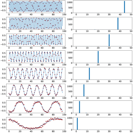
Figure 5: Cosine shape of the trained embeddings (hidden layer weights) and corresponding power of Fourier spectrum. The two-layer network with $m=1536$ neurons is trained on $k=3$-sum mod-$p=97$ addition dataset. We even split the whole datasets ($p^{k}=97^{3}$ data points) into the training and test datasets. Every row represents a random neuron from the network. The left figure shows the final trained embeddings, with red dots indicating the true weight values, and the pale blue interpolation is achieved by identifying the function that shares the same Fourier spectrum. The right figure shows their Fourier power spectrum. The results in these figures are consistent with our analysis statements in Lemma 4.2.

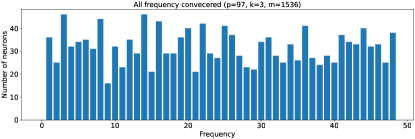
Figure 6: All Fourier spectrum frequencies being covered and the maximum normalized power of the embeddings (hidden layer weights). The one-hidden layer network with $m=1536$ neurons is trained on $k=3$-sum mod-$p=97$ addition dataset. We denote $\widehat{u}[i]$ as the Fourier transform of $u[i]$. Let $\max_{i}|\widehat{u}[i]|^{2}/(\sum|\widehat{u}[j]|^{2})$ be the maximum normalized power. Mapping each neuron to its maximum normalized power frequency, (a) shows the final frequency distribution of the embeddings. Similar to our construction analysis in Lemma 4.3, we have an almost uniform distribution over all frequencies. (b) shows the maximum normalized power of the neural network with random initialization. (c) shows, in frequency space, the embeddings of the final trained network are one-sparse, i.e., maximum normalized power being almost 1 for all neurons. This is consistent with our maximum-margin analysis results in Lemma 4.3.

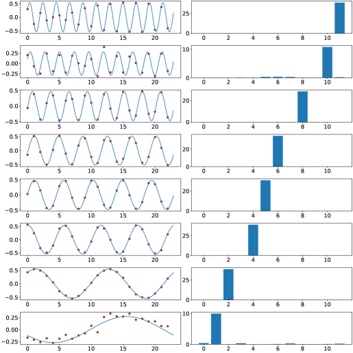
Figure 7: Cosine shape of the trained embeddings (hidden layer weights) and corresponding power of Fourier spectrum. The two-layer network with $m=5632$ neurons is trained on $k=5$-sum mod-$p=23$ addition dataset. We even split the whole datasets ($p^{k}=23^{5}$ data points) into the training and test datasets. Every row represents a random neuron from the network. The left figure shows the final trained embeddings, with red dots indicating the true weight values, and the pale blue interpolation is achieved by identifying the function that shares the same Fourier spectrum. The right figure shows their Fourier power spectrum. The results in these figures are consistent with our analysis statements in Lemma 4.2.

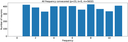
Figure 8: All Fourier spectrum frequencies being covered and the maximum normalized power of the embeddings (hidden layer weights). The one-hidden layer network with $m=5632$ neurons is trained on $k=5$-sum mod-$p=23$ addition dataset. We denote $\widehat{u}[i]$ as the Fourier transform of $u[i]$. Let $\max_{i}|\widehat{u}[i]|^{2}/(\sum|\widehat{u}[j]|^{2})$ be the maximum normalized power. Mapping each neuron to its maximum normalized power frequency, (a) shows the final frequency distribution of the embeddings. Similar to our construction analysis in Lemma 4.3, we have an almost uniform distribution over all frequencies. (b) shows the maximum normalized power of the neural network with random initialization. (c) shows, in frequency space, the embeddings of the final trained network are one-sparse, i.e., maximum normalized power being almost 1 for all neurons. This is consistent with our maximum-margin analysis results in Lemma 4.3.

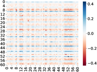
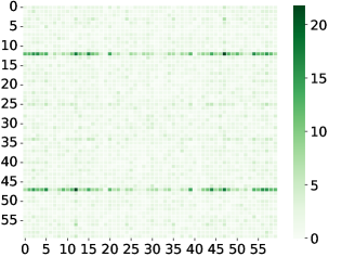
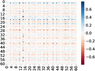
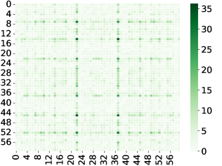
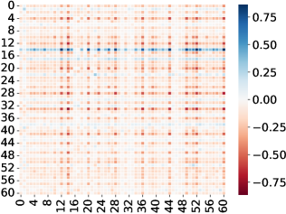
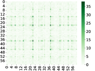
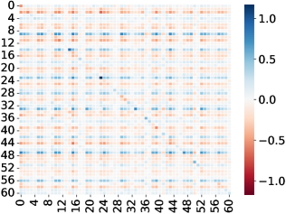
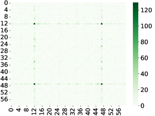
Figure 9: 2-dimension cosine shape of the trained $W^{KQ}$ (attention weights) and their Fourier power spectrum. The one-layer transformer with attention heads $m=160$ is trained on $k=3$-sum mod-$p=61$ addition dataset. We even split the whole datasets ($p^{k}=61^{3}$ data points) into training and test datasets. Every row represents a random attention head from the transformer. The left figure shows the final trained attention weights being an apparent 2-dim cosine shape. The right figure shows their 2-dim Fourier power spectrum. The results in these figures are consistent with Figure 5.

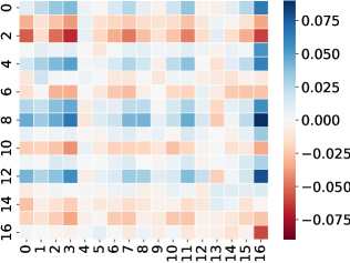
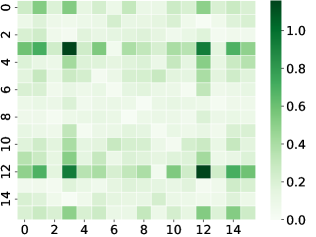
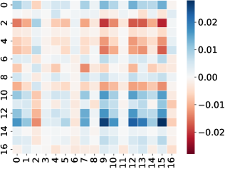
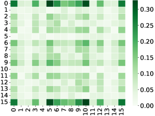
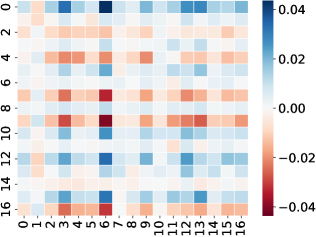
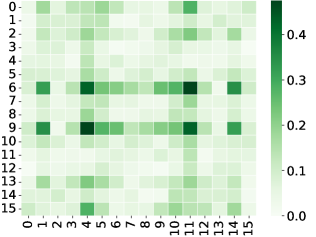
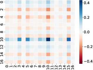
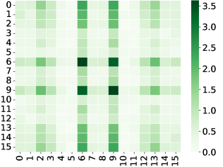
Figure 10: 2-dimension cosine shape of the trained $W^{KQ}$ (attention weights) and their Fourier power spectrum. The one-layer transformer with attention heads $m=160$ is trained on $k=5$-sum mod-$p=17$ addition dataset. We even split the whole datasets ($p^{k}=17^{5}$ data points) into training and test datasets. Every row represents a random attention head from the transformer. The left figure shows the final trained attention weights being an apparent 2-dim cosine shape. The right figure shows their 2-dim Fourier power spectrum. The results in these figures are consistent with Figure 7.

References

• AS [23] Josh Alman and Zhao Song. Fast attention requires bounded entries. In NeurIPS. arXiv preprint arXiv:2302.13214, 2023.
• AS [24] Josh Alman and Zhao Song. How to capture higher-order correlations? generalizing matrix softmax attention to kronecker computation. In The Twelfth International Conference on Learning Representations, 2024.
• BBG [22] Ido Bronstein, Alon Brutzkus, and Amir Globerson. On the inductive bias of neural networks for learning read-once dnfs. In Uncertainty in Artificial Intelligence, pages 255–265. PMLR, 2022.
• BEG+ [22] Boaz Barak, Benjamin Edelman, Surbhi Goel, Sham Kakade, Eran Malach, and Cyril Zhang. Hidden progress in deep learning: Sgd learns parities near the computational limit. Advances in Neural Information Processing Systems, 35:21750–21764, 2022.
• Bel [22] Yonatan Belinkov. Probing classifiers: Promises, shortcomings, and advances. Computational Linguistics, 48(1):207–219, March 2022.
• BFJ+ [94] Avrim Blum, Merrick Furst, Jeffrey Jackson, Michael Kearns, Yishay Mansour, and Steven Rudich. Weakly learning dnf and characterizing statistical query learning using fourier analysis. In Proceedings of the twenty-sixth annual ACM symposium on Theory of computing, pages 253–262, 1994.
• BLLT [20] Peter L Bartlett, Philip M Long, Gábor Lugosi, and Alexander Tsigler. Benign overfitting in linear regression. Proceedings of the National Academy of Sciences, 117(48):30063–30070, 2020.
• Bou [14] Jean Bourgain. An improved estimate in the restricted isometry problem. In Geometric aspects of functional analysis, pages 65–70. Springer, 2014.
• BV [04] Stephen P Boyd and Lieven Vandenberghe. Convex optimization. Cambridge university press, 2004.
• CB [20] Lenaic Chizat and Francis Bach. Implicit bias of gradient descent for wide two-layer neural networks trained with the logistic loss. In Conference on Learning Theory. PMLR, 2020.
• CCBG [22] Yuan Cao, Zixiang Chen, Misha Belkin, and Quanquan Gu. Benign overfitting in two-layer convolutional neural networks. Advances in neural information processing systems, 35:25237–25250, 2022.
• CCN [23] Bilal Chughtai, Lawrence Chan, and Neel Nanda. A toy model of universality: Reverse engineering how networks learn group operations. arXiv preprint arXiv:2302.03025, 2023.
• CGC+ [20] Nick Cammarata, Gabriel Goh, Shan Carter, Ludwig Schubert, Michael Petrov, and Chris Olah. Curve detectors. Distill, 5(6):e00024–003, 2020.
• CKPS [16] Xue Chen, Daniel M Kane, Eric Price, and Zhao Song. Fourier-sparse interpolation without a frequency gap. In 2016 IEEE 57th Annual Symposium on Foundations of Computer Science (FOCS), pages 741–750. IEEE, 2016.
• CLS [20] Sitan Chen, Jerry Li, and Zhao Song. Learning mixtures of linear regressions in subexponential time via fourier moments. In Proceedings of the 52nd Annual ACM SIGACT Symposium on Theory of Computing, pages 587–600, 2020.
• CND+ [22] Aakanksha Chowdhery, Sharan Narang, Jacob Devlin, Maarten Bosma, Gaurav Mishra, Adam Roberts, Paul Barham, Hyung Won Chung, Charles Sutton, Sebastian Gehrmann, et al. Palm: Scaling language modeling with pathways. arXiv preprint arXiv:2204.02311, 2022.
• CSS+ [23] Xiang Chen, Zhao Song, Baocheng Sun, Junze Yin, and Danyang Zhuo. Query complexity of active learning for function family with nearly orthogonal basis. arXiv preprint arXiv:2306.03356, 2023.
• CT [06] Emmanuel J Candes and Terence Tao. Near-optimal signal recovery from random projections: Universal encoding strategies? IEEE transactions on information theory, 52(12):5406–5425, 2006.
• DCLT [18] Jacob Devlin, Ming-Wei Chang, Kenton Lee, and Kristina Toutanova. Bert: Pre-training of deep bidirectional transformers for language understanding. arXiv preprint arXiv:1810.04805, 2018.
• DLS [22] Alexandru Damian, Jason Lee, and Mahdi Soltanolkotabi. Neural networks can learn representations with gradient descent. In Conference on Learning Theory. PMLR, 2022.
• DM [20] Amit Daniely and Eran Malach. Learning parities with neural networks. Advances in Neural Information Processing Systems, 33:20356–20365, 2020.
• EHO+ [22] Nelson Elhage, Tristan Hume, Catherine Olsson, Nicholas Schiefer, Tom Henighan, Shauna Kravec, Zac Hatfield-Dodds, Robert Lasenby, Dawn Drain, Carol Chen, et al. Toy models of superposition. arXiv preprint arXiv:2209.10652, 2022.
• ENO+ [21] Nelson Elhage, Neel Nanda, Catherine Olsson, Tom Henighan, Nicholas Joseph, Ben Mann, Amanda Askell, Yuntao Bai, Anna Chen, Tom Conerly, et al. A mathematical framework for transformer circuits. Transformer Circuits Thread, 1, 2021.
• FCB [22] Spencer Frei, Niladri S Chatterji, and Peter Bartlett. Benign overfitting without linearity: Neural network classifiers trained by gradient descent for noisy linear data. In Conference on Learning Theory, pages 2668–2703. PMLR, 2022.
• FVB+ [22] Spencer Frei, Gal Vardi, Peter Bartlett, Nathan Srebro, and Wei Hu. Implicit bias in leaky relu networks trained on high-dimensional data. In The Eleventh International Conference on Learning Representations, 2022.
• FVBS [23] Spencer Frei, Gal Vardi, Peter Bartlett, and Nathan Srebro. Benign overfitting in linear classifiers and leaky relu networks from kkt conditions for margin maximization. In The Thirty Sixth Annual Conference on Learning Theory, pages 3173–3228. PMLR, 2023.
• GHG+ [20] Peng Gao, Chiori Hori, Shijie Geng, Takaaki Hori, and Jonathan Le Roux. Multi-pass transformer for machine translation. arXiv preprint arXiv:2009.11382, 2020.
• [28] Suriya Gunasekar, Jason Lee, Daniel Soudry, and Nathan Srebro. Characterizing implicit bias in terms of optimization geometry. In International Conference on Machine Learning, pages 1832–1841. PMLR, 2018.
• [29] Suriya Gunasekar, Jason D Lee, Daniel Soudry, and Nati Srebro. Implicit bias of gradient descent on linear convolutional networks. Advances in Neural Information Processing Systems, 31, 2018.
• GMS [05] Anna C Gilbert, Shan Muthukrishnan, and Martin Strauss. Improved time bounds for near-optimal sparse fourier representations. In Wavelets XI, volume 5914, page 59141A. International Society for Optics and Photonics, 2005.
• GSS [22] Yeqi Gao, Zhao Song, and Baocheng Sun. An ${O}(k\log n)$ time fourier set query algorithm. arXiv preprint arXiv:2208.09634, 2022.
• HBK+ [21] Dan Hendrycks, Collin Burns, Saurav Kadavath, Akul Arora, Steven Basart, Eric Tang, Dawn Song, and Jacob Steinhardt. Measuring mathematical problem solving with the math dataset. arXiv preprint arXiv:2103.03874, 2021.
• [33] Haitham Hassanieh, Piotr Indyk, Dina Katabi, and Eric Price. Nearly optimal sparse fourier transform. In Proceedings of the forty-fourth annual ACM symposium on Theory of Computing (STOC), pages 563–578, 2012.
• [34] Haitham Hassanieh, Piotr Indyk, Dina Katabi, and Eric Price. Simple and practical algorithm for sparse fourier transform. In Proceedings of the twenty-third annual ACM-SIAM symposium on Discrete Algorithms (SODA), pages 1183–1194. SIAM, 2012.
• HR [17] Ishay Haviv and Oded Regev. The restricted isometry property of subsampled fourier matrices. In Geometric aspects of functional analysis, pages 163–179. Springer, 2017.
• IK [14] Piotr Indyk and Michael Kapralov. Sample-optimal Fourier sampling in any constant dimension. In IEEE 55th Annual Symposium onFoundations of Computer Science (FOCS), pages 514–523. IEEE, 2014.
• IKP [14] Piotr Indyk, Michael Kapralov, and Eric Price. (nearly) sample-optimal sparse fourier transform. In Proceedings of the twenty-fifth annual ACM-SIAM symposium on Discrete algorithms (SODA), pages 480–499. SIAM, 2014.
• Jac [22] Arthur Jacot. Implicit bias of large depth networks: a notion of rank for nonlinear functions. In The Eleventh International Conference on Learning Representations, 2022.
• JLS [23] Yaonan Jin, Daogao Liu, and Zhao Song. Super-resolution and robust sparse continuous fourier transform in any constant dimension: Nearly linear time and sample complexity. In ACM-SIAM Symposium on Discrete Algorithms (SODA), 2023.
• JSL [22] Samy Jelassi, Michael Sander, and Yuanzhi Li. Vision transformers provably learn spatial structure. Advances in Neural Information Processing Systems, 2022.
• JT [19] Ziwei Ji and Matus Telgarsky. The implicit bias of gradient descent on nonseparable data. In Conference on Learning Theory, pages 1772–1798. PMLR, 2019.
• JT [20] Ziwei Ji and Matus Telgarsky. Directional convergence and alignment in deep learning. Advances in Neural Information Processing Systems, 33:17176–17186, 2020.
• Kap [16] Michael Kapralov. Sparse Fourier transform in any constant dimension with nearly-optimal sample complexity in sublinear time. In Symposium on Theory of Computing Conference (STOC), 2016.
• Kap [17] Michael Kapralov. Sample efficient estimation and recovery in sparse FFT via isolation on average. In 58th Annual IEEE Symposium on Foundations of Computer Science (FOCS), 2017.
• LAD+ [22] Aitor Lewkowycz, Anders Andreassen, David Dohan, Ethan Dyer, Henryk Michalewski, Vinay Ramasesh, Ambrose Slone, Cem Anil, Imanol Schlag, Theo Gutman-Solo, et al. Solving quantitative reasoning problems with language models. Advances in Neural Information Processing Systems, 35:3843–3857, 2022.
• LH [18] Ilya Loshchilov and Frank Hutter. Decoupled weight decay regularization. In International Conference on Learning Representations, 2018.
• LJL+ [24] Kaifeng Lyu, Jikai Jin, Zhiyuan Li, Simon S Du, Jason D Lee, and Wei Hu. Dichotomy of early and late phase implicit biases can provably induce grokking. In The Twelfth International Conference on Learning Representations, 2024.
• LKN+ [22] Ziming Liu, Ouail Kitouni, Niklas S Nolte, Eric Michaud, Max Tegmark, and Mike Williams. Towards understanding grokking: An effective theory of representation learning. Advances in Neural Information Processing Systems, 35:34651–34663, 2022.
• LL [19] Kaifeng Lyu and Jian Li. Gradient descent maximizes the margin of homogeneous neural networks. In International Conference on Learning Representations, 2019.
• LLR [23] Yuchen Li, Yuanzhi Li, and Andrej Risteski. How do transformers learn topic structure: Towards a mechanistic understanding. In Proceedings of the 40th International Conference on Machine Learning, Proceedings of Machine Learning Research. PMLR, 2023.
• LLWA [21] Kaifeng Lyu, Zhiyuan Li, Runzhe Wang, and Sanjeev Arora. Gradient descent on two-layer nets: Margin maximization and simplicity bias. Advances in Neural Information Processing Systems, 34:12978–12991, 2021.
• LSX+ [22] Renqian Luo, Liai Sun, Yingce Xia, Tao Qin, Sheng Zhang, Hoifung Poon, and Tie-Yan Liu. Biogpt: generative pre-trained transformer for biomedical text generation and mining. Briefings in Bioinformatics, 23(6), 2022.
• LSZ [19] Yin Tat Lee, Zhao Song, and Qiuyi Zhang. Solving empirical risk minimization in the current matrix multiplication time. In COLT, 2019.
• LWLC [23] Hongkang Li, Meng Wang, Sijia Liu, and Pin-Yu Chen. A theoretical understanding of shallow vision transformers: Learning, generalization, and sample complexity. In The Eleventh International Conference on Learning Representations, 2023.
• MEO+ [24] Depen Morwani, Benjamin L Edelman, Costin-Andrei Oncescu, Rosie Zhao, and Sham Kakade. Feature emergence via margin maximization: case studies in algebraic tasks. In The Twelfth International Conference on Learning Representations, 2024.
• Mil [22] Beren Millidge. Grokking’grokking’, 2022.
• Moi [15] Ankur Moitra. Super-resolution, extremal functions and the condition number of vandermonde matrices. In Proceedings of the forty-seventh annual ACM symposium on Theory of computing, pages 821–830, 2015.
• MSAM [23] Shikhar Murty, Pratyusha Sharma, Jacob Andreas, and Christopher D Manning. Grokking of hierarchical structure in vanilla transformers. arXiv preprint arXiv:2305.18741, 2023.
• MWG+ [20] Edward Moroshko, Blake E Woodworth, Suriya Gunasekar, Jason D Lee, Nati Srebro, and Daniel Soudry. Implicit bias in deep linear classification: Initialization scale vs training accuracy. Advances in Neural Information Processing Systems, 33, 2020.
• NCL+ [23] Neel Nanda, Lawrence Chan, Tom Lieberum, Jess Smith, and Jacob Steinhardt. Progress measures for grokking via mechanistic interpretability. In The Eleventh International Conference on Learning Representations, 2023.
• NSW [19] Vasileios Nakos, Zhao Song, and Zhengyu Wang. (nearly) sample-optimal sparse fourier transform in any dimension; ripless and filterless. In 2019 IEEE 60th Annual Symposium on Foundations of Computer Science (FOCS), pages 1568–1577. IEEE, 2019.
• OCS+ [20] Chris Olah, Nick Cammarata, Ludwig Schubert, Gabriel Goh, Michael Petrov, and Shan Carter. Zoom in: An introduction to circuits. Distill, 5(3):e00024–001, 2020.
• OEN+ [22] Catherine Olsson, Nelson Elhage, Neel Nanda, Nicholas Joseph, Nova DasSarma, Tom Henighan, Ben Mann, Amanda Askell, Yuntao Bai, Anna Chen, et al. In-context learning and induction heads. arXiv preprint arXiv:2209.11895, 2022.
• Ope [22] OpenAI. Introducing ChatGPT. https://openai.com/blog/chatgpt, 2022. Accessed: 2023-09-10.
• Ope [23] OpenAI. Gpt-4 technical report, 2023.
• PBE+ [22] Alethea Power, Yuri Burda, Harri Edwards, Igor Babuschkin, and Vedant Misra. Grokking: Generalization beyond overfitting on small algorithmic datasets. arXiv preprint arXiv:2201.02177, 2022.
• PCR [20] Gabriele Prato, Ella Charlaix, and Mehdi Rezagholizadeh. Fully quantized transformer for machine translation. In Findings of the Association for Computational Linguistics: EMNLP 2020, pages 1–14, 2020.
• PS [15] Eric Price and Zhao Song. A robust sparse Fourier transform in the continuous setting. In 2015 IEEE 56th Annual Symposium on Foundations of Computer Science, pages 583–600. IEEE, 2015.
• RV [08] Mark Rudelson and Roman Vershynin. On sparse reconstruction from fourier and gaussian measurements. Communications on Pure and Applied Mathematics: A Journal Issued by the Courant Institute of Mathematical Sciences, 61(8):1025–1045, 2008.
• SCL+ [23] Zhenmei Shi, Jiefeng Chen, Kunyang Li, Jayaram Raghuram, Xi Wu, Yingyu Liang, and Somesh Jha. The trade-off between universality and label efficiency of representations from contrastive learning. In The Eleventh International Conference on Learning Representations, 2023.
• SGHK [18] David Saxton, Edward Grefenstette, Felix Hill, and Pushmeet Kohli. Analysing mathematical reasoning abilities of neural models. In International Conference on Learning Representations, 2018.
• SHN+ [18] Daniel Soudry, Elad Hoffer, Mor Shpigel Nacson, Suriya Gunasekar, and Nathan Srebro. The implicit bias of gradient descent on separable data. The Journal of Machine Learning Research, 19(1):2822–2878, 2018.
• SHT [23] Clayton Sanford, Daniel Hsu, and Matus Telgarsky. Representational strengths and limitations of transformers. In Thirty-seventh Conference on Neural Information Processing Systems, 2023.
• SMF+ [23] Zhenmei Shi, Yifei Ming, Ying Fan, Frederic Sala, and Yingyu Liang. Domain generalization via nuclear norm regularization. In Conference on Parsimony and Learning (Proceedings Track), 2023.
• Son [19] Zhao Song. Matrix Theory: Optimization, Concentration and Algorithms. PhD thesis, The University of Texas at Austin, 2019.
• SSSS [17] Shai Shalev-Shwartz, Ohad Shamir, and Shaked Shammah. Failures of gradient-based deep learning. In International Conference on Machine Learning, pages 3067–3075. PMLR, 2017.
• SSWZ [22] Zhao Song, Baocheng Sun, Omri Weinstein, and Ruizhe Zhang. Sparse fourier transform over lattices: A unified approach to signal reconstruction. arXiv preprint arXiv:2205.00658, 2022.
• SSWZ [23] Zhao Song, Baocheng Sun, Omri Weinstein, and Ruizhe Zhang. Quartic samples suffice for fourier interpolation. In 2023 IEEE 64th Annual Symposium on Foundations of Computer Science (FOCS), pages 1414–1425. IEEE, 2023.
• STR+ [20] Harshay Shah, Kaustav Tamuly, Aditi Raghunathan, Prateek Jain, and Praneeth Netrapalli. The pitfalls of simplicity bias in neural networks. Advances in Neural Information Processing Systems, 33:9573–9585, 2020.
• SWL [22] Zhenmei Shi, Junyi Wei, and Yingyu Liang. A theoretical analysis on feature learning in neural networks: Emergence from inputs and advantage over fixed features. In International Conference on Learning Representations, 2022.
• SWL [23] Zhenmei Shi, Junyi Wei, and Yingyu Liang. Provable guarantees for neural networks via gradient feature learning. In Thirty-seventh Conference on Neural Information Processing Systems, 2023.
• SWXL [23] Zhenmei Shi, Junyi Wei, Zhuoyan Xu, and Yingyu Liang. Why larger language models do in-context learning differently? In R0-FoMo:Robustness of Few-shot and Zero-shot Learning in Large Foundation Models, 2023.
• SYYZ [23] Zhao Song, Mingquan Ye, Junze Yin, and Lichen Zhang. A nearly-optimal bound for fast regression with $\ell_{\infty}$, guarantee. In ICML, volume 202 of Proceedings of Machine Learning Research, pages 32463–32482. PMLR, 2023.
• TB [23] Alexander Tsigler and Peter L Bartlett. Benign overfitting in ridge regression. Journal of Machine Learning Research, 24(123):1–76, 2023.
• TLZ+ [22] Vimal Thilak, Etai Littwin, Shuangfei Zhai, Omid Saremi, Roni Paiss, and Joshua Susskind. The slingshot mechanism: An empirical study of adaptive optimizers and the grokking phenomenon. arXiv preprint arXiv:2206.04817, 2022.
• TMS+ [23] Hugo Touvron, Louis Martin, Kevin Stone, Peter Albert, Amjad Almahairi, Yasmine Babaei, Nikolay Bashlykov, Soumya Batra, Prajjwal Bhargava, Shruti Bhosale, et al. Llama 2: Open foundation and fine-tuned chat models. arXiv preprint arXiv:2307.09288, 2023.
• TWCD [23] Yuandong Tian, Yiping Wang, Beidi Chen, and Simon Du. Scan and snap: Understanding training dynamics and token composition in 1-layer transformer. Advances in Neural Information Processing Systems, 2023.
• Var [23] Gal Vardi. On the implicit bias in deep-learning algorithms. Communications of the ACM, 66(6):86–93, 2023.
• [89] Colin Wei, Jason D Lee, Qiang Liu, and Tengyu Ma. Regularization matters: Generalization and optimization of neural nets vs their induced kernel. Advances in Neural Information Processing Systems, 32, 2019.
• [90] Colin Wei, Jason D Lee, Qiang Liu, and Tengyu Ma. Regularization matters: Generalization and optimization of neural nets vs their induced kernel. Advances in Neural Information Processing Systems, 32, 2019.
• WTB+ [22] Jason Wei, Yi Tay, Rishi Bommasani, Colin Raffel, Barret Zoph, Sebastian Borgeaud, Dani Yogatama, Maarten Bosma, Denny Zhou, Donald Metzler, Ed H. Chi, Tatsunori Hashimoto, Oriol Vinyals, Percy Liang, Jeff Dean, and William Fedus. Emergent abilities of large language models. Transactions on Machine Learning Research, 2022.
• XSW+ [23] Zhuoyan Xu, Zhenmei Shi, Junyi Wei, Yin Li, and Yingyu Liang. Improving foundation models for few-shot learning via multitask finetuning. In ICLR 2023 Workshop on Mathematical and Empirical Understanding of Foundation Models, 2023.
• XSW+ [24] Zhuoyan Xu, Zhenmei Shi, Junyi Wei, Fangzhou Mu, Yin Li, and Yingyu Liang. Towards few-shot adaptation of foundation models via multitask finetuning. In The Twelfth International Conference on Learning Representations, 2024.
• XWF+ [24] Zhiwei Xu, Yutong Wang, Spencer Frei, Gal Vardi, and Wei Hu. Benign overfitting and grokking in relu networks for xor cluster data. In The Twelfth International Conference on Learning Representations, 2024.
• YC [23] Roozbeh Yousefzadeh and Xuenan Cao. Large language models’ understanding of math: Source criticism and extrapolation. arXiv preprint arXiv:2311.07618, 2023.