Optimal Thresholding Linear Bandit
Abstract
We study a novel pure exploration problem: the -Thresholding Bandit Problem (TBP) with fixed confidence in stochastic linear bandits. We prove a lower bound for the sample complexity and extend an algorithm designed for Best Arm Identification in the linear case to TBP that is asymptotically optimal.
1 Introduction
The Thresholding Bandit Problem (TBP) Andrea Locatelli (2016); Kano et al. (2019) represents a specific combinatorial pure exploration problem Wei Chen (2013) within the stochastic bandit setting. In this problem, the learner’s objective is to identify all arms whose mean reward is above a specified threshold .
The study by Kano et al. (2019) emphasizes that in certain contexts, such as personalized recommendations, pursuing the absolute best option might not always align with the most advantageous objective. Rather, the pursuit of viable alternatives could yield greater benefits. This concept extends to domains like scientific discoveries, such as in chemical reactions, where the primary focus might not solely revolve around identifying the single best reaction, but rather maximizing the discovery of multiple favorable reactions. Given the perceived value in practical applications, our objective is to advance our understanding of TBP, particularly within the framework of structured bandits.
On the other hand, the stochastic linear bandit Auer (2002) is a sequential decision-making problem that extends the classical stochastic Multi-Armed Bandit Robbins (1952). In this scenario, the arms’ mean rewards follow a linear model with unknown parameters. While much of the analysis of this problem has focused on the regret minimization objective Paat Rusmevichientong (2010); Yasin Abbasi-Yadkori (2011), some research has addressed it within the context of the best-arm identification (BAI) problem Marta Soare (2014); Soare (2015); Yassir Jedra (2020); Degenne et al. (2020).
1.1 Contributions
In this paper we explore the understudied -TBP in stochastic linear bandits and make the following key contributions.
-
•
We prove an instance-specific lower bound for the expected sample complexity of any correct algorithm.
-
•
We extend the algorithm of Yassir Jedra (2020) to the TBP and prove it is asymptotically optimal. The main difference is that their algorithm focuses on sampling arms to reduce uncertainty, particularly for arms that are harder to distinguish from the optimal arm (i.e., arms with mean rewards very close to each other) whereas ours pays attention to arms with mean rewards close to the threshold .
-
•
Moreover, we are able to modify the algorithm for the -relaxed case. While Track and Stop algorithms can fail for problems with multiple correct solutions if the set of optimal solutions is not convex, as discussed by Degenne and Koolen (2019), we demonstrate that the set of optimal proportions is convex and hencwe we can guarantee asymptotic optimality.
1.2 Related work
In the context of the combinatorial pure exploration (CPE) problem, the learner’s goal is to explore a set of arms to identify the optimal member of a decision class. Wei Chen (2013) introduced general algorithms to address CPE in both fixed confidence and fixed budget settings. Andrea Locatelli (2016) provided a formal definition of the Thresholding Bandit Problem (TBP), along with a summary of lower and upper bounds in the fixed confidence and budget settings. Notably, they presented an algorithm that matches the lower bound of the error probability up to multiplicative constants, and additive terms, in the exponential.
In the realm of fixed confidence, Kano et al. (2019) formulated the Good Arm Identification (GAI) problem, where the learner selects good arms, defined as arms with mean rewards above a specified threshold, one by one.
Marta Soare (2014) was the first to introduce Best-Arm Identification (BAI) in the stochastic linear setting and derived an instance-specific information-theoretical lower bound for the expected sample complexity. They offered static and adaptive algorithms inspired by G-optimal experimental design. Tao et al. (2018) introduced an elimination-based algorithm that improved upon the previous upper bound established by Marta Soare (2014). In Xu et al. (2018), they designed the first gap-based algorithm for BAI in the linear case, drawing inspiration from UGapE Gabillon et al. (2012).
Furthermore, Yassir Jedra (2020) presented an asymptotically optimal algorithm based on the classic Track and Stop algorithm for BAI in the Multi-Armed Bandit (MAB) setting Garivier and Kaufmann (2016). Meanwhile, Degenne et al. (2020) introduced a general pure exploration formulation for the linear case, focusing on single answers. They provided the asymptotic lower bound for sample complexity and an asymptotically optimal algorithm. Their approach treats the problem as a two-player zero-sum game, with the algorithm solving a saddle point to approximate the optimal proportions determined by the problem’s complexity.
2 Problem Formulation
Consider a set of arms , each associated with a feature vector , , and an unknown parameter vector . We assume that for all , where . In round , the decision maker selects arm and she observes reward , where and is independent of the past observations. We denote the history as and the filtration generated for this history as .
A pure exploration algorithm comprises a sampling rule , a stopping rule and a decision rule . The sampling rule determines the action taken in round and can be randomized. Therefore, if we denote the set of all the distributions over , each is a mapping from history to , i.e. is measurable and . The stopping rule is the time when the learner stops sampling and makes the decision. Thus, has to be a stopping time with respect to . The decision rule is measurable and it is a subset of according with some optimality criteria.
In our case, given a threshold and a fixed confidence , the objective of the learner is to find all the arms with mean reward above in the least time possible with probability at least . Formally, let . We will omit the subscript when it is clear .
Definition 2.1.
We say that the tuple is -correct if:
and
We can also introduce a relaxation of the threshold condition, permitting the misidentification of arms within an radius, where , around the threshold.
We can also relax the threshold condition, allowing arms to be misidentified within an radius, where , around the threshold.
Definition 2.2.
We say that the tuple is -correct if:
and
As we will see, relaxing the threshold criteria reduces the complexity of the problem. We will use the natural choice for the decision rule , where is the least squares estimator of at the stopping time.
3 Sample Complexity Lower Bound
3.1 Geometric Intuition
Stopping rule
For the sake of gaining intuition about how well an algorithm can perform, we assume we can use the knowledge of the true to construct confidence set and then define the sample and stopping rules. This will show that even an “oracle" strategy needs a minimum sample size to be confident enough about the answer. Furthermore, it will help to understand how TBP it is different from the BAI in the linear case.
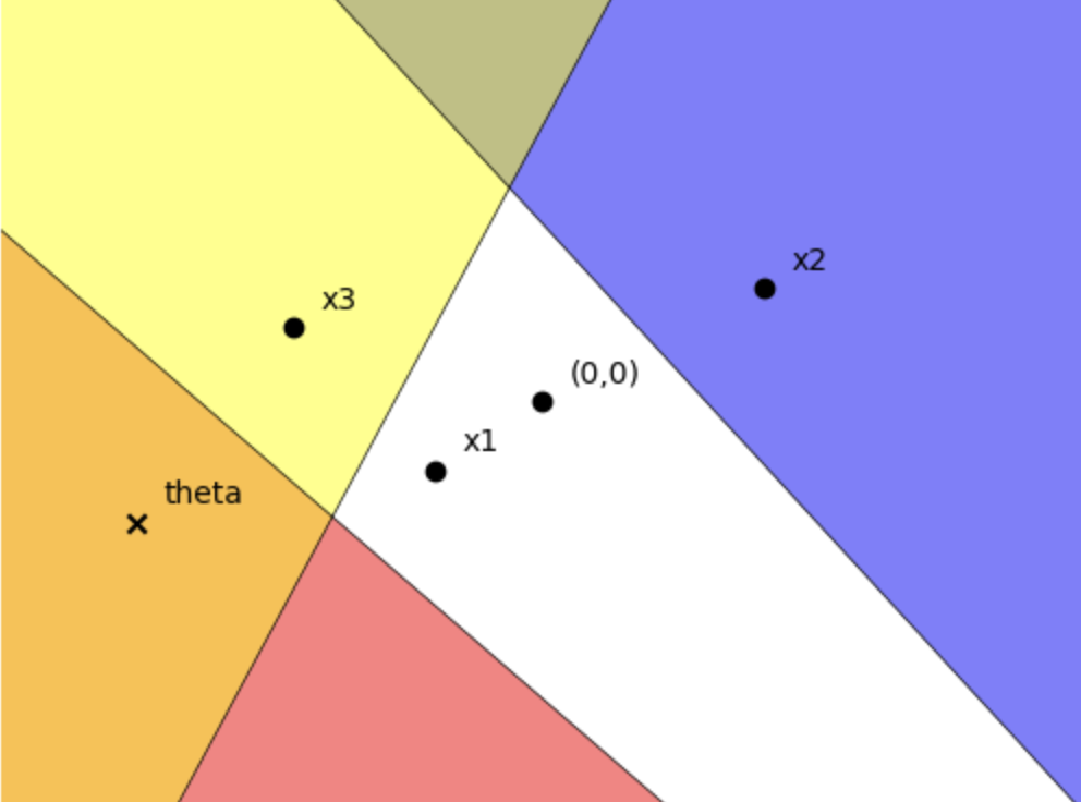
First, following Marta Soare (2014), let the set of parameters that makes have a mean reward above . This sets are open half spaces.
In contrast to Marta Soare (2014), our definition of does not form a partition of . Instead, the true parameter resides at the intersection of for all the "good arms", i.e. . Furthermore, . Note that all have the same .
As in Marta Soare (2014), we assume that for any allocation , it is possible to construct a confidence set such that and the (random) OLS estimate belongs to with high probability, i.e., . As a result, the oracle stopping criterion simply checks whether the confidence set is contained in both and . That means, for all the probable values of , there is no ambiguity about the arms that are above/below the threshold.
Proposition 3.1.
Let be an allocation such that , then
Proof.
The proof follows immediately because of the fact that with probability at least , then and this implies that . ∎
Sampling rule
From the previous arguments, it is evident that the goal of the optimal strategy should be to shrink the confidence set such that as quick as possible. Formally, is equivalent to
where . Then we can define our confidence set
Where and for some . Thus the stopping condition is equivalent to
For all . From this condition, the oracle allocation strategy simply follows
Sample complexity
Now we can define the sample complexity as the minimum number of samples we need to meet the stopping time condition.
Note that we can formulate this problem as an optimal design (soft allocation) replacing with . Then, if we denote the problem complexity
Then, we can choose such that with probability at least Yasin Abbasi-Yadkori (2011)
3.2 Lower bound
The geometric intuition provides valuable insights into the sample complexity lower bound and problem complexity. As we will see, we can leverage standard BAI concepts to establish a non-asymptotic lower bound. Similar to the linear case in BAI, the lower bound for the sample complexity is determined by the optimization problem involving the ratio of the norm induced by the inverse of the design and the gaps . In our setting the gaps are defined as the distance between the mean rewards and the threshold.
It’s worth noting that Degenne et al. (2020) established a general asymptotic lower bound for pure exploration problems in the context of stochastic linear bandits, and our lower bound aligns with their findings. We extend this result to a more general setting for thresholding bandits, encompassing the relaxed version of the problem outlined in Definition 2.1.
Theorem 3.2.
For any linear bandit environment , the sample complexity of any --correct tuple strategy satisfies:
where , , captures the sample repartition over the arms , as given by the design , is the gap.
Proof.
We will follow the usual approach for lower bound for the sample complexity introduce in (Garivier and Kaufmann, 2016). Denote by the binary relative entropy. Let a different bandit enviroment such that for which and or and , i.e. or .
Then consider the event , because the tuples are --correct we have:
Using Lemma 1 from (Garivier and Kaufmann, 2016) we have
Let’s consider that allows to maximize the lower bound. Then, the condition that the two environments have different set of good arms is equivalent to:
For some or
For some . The smallest satisfying this condition is given by the solution of the following (relaxed) minimization problem. Denote , the arms that are outside radius interval of .
Now we can use the same approach as in Theorem 3.1. (Soare, 2015).
Then
∎
Corollary 3.3.
For any linear bandit environment , the sample complexity of any -correct tuple strategy satisfies:
where and is the gap.
4 Algorithm
The goal of this section is to introduce a method that achieves asymptotic optimality. We will adopt the conventional Track and Stop strategy for BAI, initially introduced by Garivier and Kaufmann (2016). The primary aim of this strategy is to estimate and align with the optimal proportions that lead to asymptotically optimal sample complexity. It is important to note that in the relaxed setting, the issue of multiple correct answers can arise (Degenne and Koolen, 2019). However, we demonstrate that for this setting, the set of optimal proportions is also convex. As a result, we ensure that the Track and Stop algorithm will converge within the convex hull of optimal solutions, maintaining optimality.
The primary distinction between the stochastic linear bandits case and the traditional Multi-Armed Bandit (MAB) lies in how to compute the optimal proportions. These proportions are dictated by the problem’s complexity. Interestingly, in the case of linear rewards, this strategy also proves effective for TBP.
Furthermore, we can take advantage of the advancements in lazy updates as introduced by Yassir Jedra (2020). These updates help alleviate the computational burden of recalculating the optimal proportions at each iteration.
4.1 Least-squares estimator
Our algorithm employs the ordinary least-squares (OLS) estimator. In order to apply the concentration inequalities from Yasin Abbasi-Yadkori (2011) we need to establish a modified version. Instead of relying on the regularized least-squares estimator, we enforce exploration, as demonstrated by Yassir Jedra (2020). It appears that initializing the OLS estimator with linearly independent arms is sufficient to utilize the confidence ellipsoid from the theorem in Yasin Abbasi-Yadkori (2011), albeit with a modification in the upper bound.
Let , , , then is the OLS estimator with the observations until time . We have the following Lemma
Lemma 4.1.
Let be a filtration. Let be a real-valued stochastic process such that is -measurable, -conditionally -sub-Gaussian for some . Let be an -valued stochastic process such that is -measurable. Assume that exists such that for all , is a positive definite matrix, i.e. and with for some . Then, for any , with probability at least , for all ,
And then for all
4.2 Sampling Rule
We will aim to match the optimal proportions from the optimization problem defined in the lower bound analysis. Denote
We prove that is equivalent to:
(see proof of Theorem 3.2). To guarantee we can solve this optimization problem and the solution will produce an strategy with optimal sample complexity we need two lemmas. These lemmas are proved by Yassir Jedra (2020) for BAI, we will adapt them to TBP.
Lemma 4.2.
is continuous in both and , and attains its maximum in at a point such that is invertible.
Lemma 4.3.
(Maximum theorem) Let . Define and . Then is continuous at , and is convex, compact and non-empty. Furthermore, we have for any open neighborhood of , there exists an open neighborhood of , such that for all , we have .
As emphasized by Garivier and Kaufmann (2016), in stochastic bandits, directly substituting estimated parameters can be perilous. Therefore, we cannot utilize the optimal proportion directly. Instead, we employ the forced exploration sampling method proposed by Yassir Jedra (2020).
Lemma 4.4.
(Lemma 5 (Yassir Jedra, 2020)) Let . Let be an arbitrary sequence of arms. Furthermore, define for all where . Consider the sampling rule, defined recursively as: , and for , and
| (1) |
Then for all , we have .
Lemma 4.5.
In Degenne et al. (2020), they also attempt to align with the optimal proportions established by an equivalent saddle point. However, they adopt an optimistic approach to deal with the uncertainty associated with .
We will leverage the Lazy update rule from Yassir Jedra (2020). Therefore, we need to ask the same conditions to guarantee almost sure asymptotical optimality and optimality in terms of expected sample complexity.
There exists a non-decreasing sequence of integers with for and and such that
| (2) |
As the authors pointed out, this condition is not hard to meet and it it enough to guarantee almost sure asymptotical optimality (see proof of Theorem 4.7). On the other hand, to obtain an algorithm with optimal expected sample complexity, we need to consider the following condition: there exist and a non-decreasing sequence of integers with and for some and such that
| (3) |
4.3 Stopping Rule
As shown in section 3.1, the goal of the algorithm is to stop when the confidence set for the parameter has no ambiguity about the correct answer. This can be expressed as
| (4) |
| (5) |
| (6) |
As noticed by previous works Garivier and Kaufmann (2016); Yassir Jedra (2020); Degenne et al. (2020), this can be interpreted as a sequential hypothesis testing that stops when the generalized likelihood ratio exceeds the threshold . Therefore, the algorithm will stop at time and will output the arms above and bellow the threshold:
Lemma 4.6.
Under any sampling rule, we have
4.4 Sample complexity analysis
In this section we establish algorithm’s asymptotic optimality both with high probability and in expectation.
Theorem 4.7.
Lazy Track-Threshold-and-Stop satisfies the same sample complexity upper bound
Theorem 4.8.
Lazy Track-Threshold-and-Stop satisfies the same sample complexity upper bound
5 Experiments
In this section we compare the performance of Lazy TTS with some algorithms from BAI in the linear case: LinGapE Xu et al. (2018), G allocation (Marta Soare, 2014), RAGE (Fiez et al., 2019). To the best of our knowledge, there is only one algorithm that addresses TBP in the linear case proposed by (Degenne et al., 2020). To have a fair comparison with algorithms designed for BAI, we will adapt them to handle the TBP. The main idea is that most of these algorithms are designed to reduce the uncertainty of the gaps between the optimal and the rest of arms . Instead, we need to reduce the uncertainty of the gaps with respect to the threshold . We implement the sampling rule of each algorithm and use the same stopping rule for all of them. Another modification we need to make is modifying the standard experiments on synthetic data.
Linear bandits: modified benchmark example. One of the benchmark examples in the linear bandit BAI literature introduced by Marta Soare (2014) is the following. Consider where is the -standard basis vector, with small, and so that . This setting results in a hard problem for BAI because the gap between and is small, which implies a large complexity of the problem. For TBP this is not necessarily a hard problem, if we choose a threshold , all arms would have a gap of almost with respect to the threshold. We proposed a slightly modified version of this setting such that it is hard to distinguish if one of the arms is above or below the threshold. Consider similar setting as before, where is the -standard basis vector, , and small. Let , , such that , for , and .
Uniform Distribution on a Sphere. In this example, is sampled from a unit sphere of dimension centered at the origin. We set randomly such that , and . To control the complexity across the experiments, we discard arms with mean reward in .
6 Summary and discussion
In this work, we establish a finite sample complexity lower bound for TBP in the linear case and present an asymptotically optimal algorithm inspired by BAI. We hope that our work helps to extend TBP to other structured frameworks, such as Generalized Linear Models. Additionally, we are interested in exploring scenarios where we can only sample each arm once. This setting is known as Active Search (AS) or Adaptive Sampling for Discovery (ASD) and has been studied for the regret minimization objective. We believe that by combining both directions, we can develop sampling strategies that accelerate scientific discoveries in situations where there is no a fixed budget, but instead we want to know when to stop sampling.
| random | lazy TTS (ours) | LinGapE | -static | RAGE | LinGame | |
|---|---|---|---|---|---|---|
| 2 | 86 | 45 | 58 | 72 | 55 | 46 |
| 5 | 266 | 69 | 92 | 362 | 261 | 100 |
| 10 | 1066 | 136 | 168 | 1240 | 818 | 217 |
| 20 | 3786 | 353 | 481 | 5299 | 1938 | 597 |
| random | lazy TTS (ours) | LinGapE | -static | RAGE | LinGame | |
|---|---|---|---|---|---|---|
| 100 | 926 | 198 | 205 | 381 | 353 | 222 |
| 200 | 1886 | 390 | 389 | 646 | 552 | 484 |
| 300 | 2324 | 424 | 448 | 681 | 563 | 528 |
| 500 | 3226 | 690 | 697 | 1144 | 959 | 844 |
| 1000 | 4236 | 792 | 725 | 1274 | 876 | 1251 |
References
- Andrea Locatelli (2016) Andrea Locatelli, A. C., Maurilio Gutzeit An optimal algorithm for the Thresholding Bandit Problem. 2016, 1690–1698.
- Kano et al. (2019) Kano, H.; Honda, J.; Sakamaki, K.; Matsuura, K.; Nakamura, A.; Sugiyama, M. Good arm identification via bandit feedback. Machine Learning 2019, 108, 721–745.
- Wei Chen (2013) Wei Chen, Y. Y., Yajun Wang Combinatorial Multi-Armed Bandit: General Framework, Results and Applications. International Conference on Machine Learning. 2013; pp 151–159.
- Auer (2002) Auer, P. Using Confidence Bounds for Exploitation-Exploration Trade-offs. Journal of Machine Learning Research 2002, 397–422.
- Robbins (1952) Robbins, H. Some aspects of the sequential design of experiments. Bulletin of the American Mathematical Society 1952, 527–535.
- Paat Rusmevichientong (2010) Paat Rusmevichientong, J. N. T. Linearly Parameterized Bandits. Mathematics of Operations Research 2010, 35.
- Yasin Abbasi-Yadkori (2011) Yasin Abbasi-Yadkori, C. S., Dávid Pál Improved algorithms for linear stochastic bandits. Advances in neural information processing systems 2011, 24, 2312–2320.
- Marta Soare (2014) Marta Soare, R., Alessandro Lazaric Best-Arm Identification in Linear Bandits. Advances in neural information processing systems 2014, 27.
- Soare (2015) Soare, M. Sequential Resource Allocation in Linear Stochastic Bandits. Sequential Resource Allocation in Linear Stochastic Bandits. 2015.
- Yassir Jedra (2020) Yassir Jedra, A. P. Optimal Best-arm Identification in Linear Bandits. Advances in neural information processing systems 2020, 33.
- Degenne et al. (2020) Degenne, R.; Menard, P.; Shang, X.; Valko, M. Gamification of Pure Exploration for Linear Bandits. Proceedings of the 37th International Conference on Machine Learning. 2020; pp 2432–2442.
- Degenne and Koolen (2019) Degenne, R.; Koolen, W. M. Pure Exploration with Multiple Correct Answers. Advances in Neural Information Processing Systems. 2019.
- Tao et al. (2018) Tao, C.; Blanco, S.; Zhou, Y. Best Arm Identification in Linear Bandits with Linear Dimension Dependency. International Conference on Machine Learning. 2018; pp 4884–4893.
- Xu et al. (2018) Xu, L.; Honda, J.; Sugiyama, M. A fully adaptive algorithm for pure exploration in linear bandits. Proceedings of the Twenty-First International Conference on Artificial Intelligence and Statistics. 2018; pp 843–851.
- Gabillon et al. (2012) Gabillon, V.; Ghavamzadeh, M.; Lazaric, A. Best Arm Identification: A Unified Approach to Fixed Budget and Fixed Confidence. Advances in Neural Information Processing Systems. 2012; pp 3212–3220.
- Garivier and Kaufmann (2016) Garivier, A.; Kaufmann, E. Optimal Best Arm Identification with Fixed Confidence. 29th Annual Conference on Learning Theory. 2016; pp 998–1027.
- Fiez et al. (2019) Fiez, T.; Jain, L.; Jamieson, K. G.; Ratliff, L. Sequential Experimental Design for Transductive Linear Bandits. Advances in Neural Information Processing Systems. 2019.
- Tor Lattimore (2018) Tor Lattimore, C. S. Bandit Algorithms; Cambridge University Press, 2018.
- Sundaram et al. (1996) Sundaram, R. K.; others A First Course in Optimization Theory; Cambridge University Press, 1996.
7 Appendix
In order to prove Lemma 4.1 we need some lemmas first.
Lemma 7.1.
(Lemma 8 from (Yasin Abbasi-Yadkori, 2011))
Let be arbitrary and consider for any
Let be a stopping time with respect to filtration . then is almost surely well defined and
Proof.
Without loss of generality, assume . Let
and
Note that and for . By Lemma Lemma 20.2 in (Tor Lattimore, 2018), is a non-negative supermartingale with . Let which is independent of all the other random variables. Define
where is the tail -algebra of the filtration. We can calculate a more explicit form of . Let be the pdf of and . Then
Note that
By Lemma 20.3 in (Tor Lattimore, 2018) is a non-negative supermartingale and we can apply the maximal inequality (Theorem 3.9 in (Tor Lattimore, 2018) )
∎
Lemma 4.1. Let be a filtration. Let be a real-valued stochastic process such that is -measurable, -conditionally -sub-Gaussian for some . Let be an -valued stochastic process such that is -measurable. Assume that exists such that for all , is a positive definite matrix, i.e. and with for some . Then, for any , with probability at least , for all ,
And then for all
Proof.
First note that
Then
On the other hand
Thus
Let , then using Lemma 7.2, we have that with probability at least
In particular for
Then
∎
Lemma 4.2.
We have:
In addition, is continuous in both and , and attains its maximum in at a point such that is invertible.
Proof.
Let such that and . Consider the set of bad parameters with respect to ,
and denote
Let be a sequence taking values in and converging to . Let , and let such that for all we have . Now, we can verify that by our choice of it holds that . Let , then (the case is analogous). Then exists such that and . Note that
Then and . Conversely, let , following similar ideas
then
and
Thus and . Furthermore, note that is a polynomial in , thus it is in in particular continuous in , and there exists such that for all and for all , it holds that . Hence, with our choice of , we have for all
Thus is continuos in . Now, we know that is continuous on , and by compactness of the simplex, the maximum is attained at some . Furthermore, since spans , we may construct an allocation such that is a positive definite matrix. In addition, by construction of , there exists some such that for all we have , which implies that . On the other hand, for any allocation such that is rank deficient, we may find a where is in the null space of . Therefore, is invertible.
∎
Lemma 4.3. (Maximum theorem) Let . Define and . Then is continuous at , and is convex, compact and non-empty. Furthermore, we have for any open neighborhood of , there exists an open neighborhood of , such that for all , we have .
Proof.
The lemma is a direct consequence of the maximum theorem (a.k.a. Berge’s theorem) (Sundaram et al., 1996) and only requires that is continuous in , that is compact, convex and non-empty, and that is concave in for each in an open neighborhood of . These requirements hold naturally in our setting: (i) by Lemma 4.2, we have for all and for any is continuous in ( ; (ii) is a non-empty, compact and convex set; (iii) for all is concave as it can be expressed as the infimum of linear functions in . Therefore, the maximum theorem applies and we obtain the desired results.
∎
Lemma 4.6.
Under any sampling rule, we have
Similarly than (Yassir Jedra, 2020), a sufficient condition to --correctness is , in that case we have
Theorem 4.7
Lazy Track-Threshold-and-Stop satisfies the same sample complexity upper bound
Proof.
holds with probability 1 (Lemma 3, 5 and Proposition 1 in (Yassir Jedra, 2020)). Let , By continuity of , there exists an open neighborhood of such that for all , it holds that
for any . Under , there exists such that for all it holds that , this for all , it follows that
By Lemma 5 in (Yassir Jedra, 2020), there exists such that for all we have
Then we can write
Hence, under and for
Then
Where the last inequality uses Leamma 8 in (Yassir Jedra, 2020). Thus
∎
Theorem 4.8
Lazy Track-Threshold-and-Stop satisfies the same sample complexity upper bound
Because the algorithms have the same nature, we will follow the proof in (Yassir Jedra, 2020) closely. We include it here for completeness.
Proof.
Let
Step 1. By continuity of (see Lemma 4.2), there exists such that for all and
| (9) |
for any (we have ). Furthermore, by the continuity properties of the correspondance (see Lemma 4.3), there exists such that for all
Let . In the following, we construct , and for each an event , under which for all , it holds
Let , and define the following events
Note that, under the event , we have for all , there exists such that
Define . By Lemma 4.5 (6 of Yassir Jedra (2020)) , there exists such that
where and more precisely (see the proof of Lemma 6 of Yassir Jedra (2020)). Thus for , we have . Hence, defining for all , the event
we have shown that for all , the following holds
| (10) |
Finally, combining the implication 10 with the fact that 9 holds under we conclude that for all , under we have
| (11) |
Step 2.: Let where is defined as
where we recall that is the constant chosen in the stopping rule and is independent of . For all we have
Thus under the event , the inequality 11 holds, and for all we have
where for some independent of . This means for , we have shown that
| (12) |
Define . We may then write for all
Taking the expectation of the above inequality, and using the set inclusion 12, we obtain that
Now we observe that
We have thus shown that
| (13) |
Step 3: We now show that and that it can be upper bounded by a constant independent of . To ensure this, we shall see that there is a minimal rate by which the sequence must grow. Let , we have by the union bound
First, using a union bound and the lazy condition 3, we observe that there exists and such that
This clearly shows that . Second, we observe, using a union bound, Lemma 5 and Lemma 4 from Yassir Jedra (2020), that there exists strictly positive constants that are independent of and , and such that
For large enough, the function becomes decreasing. Additionally, we have by assumption that is a non decreasing and that , thus we may find such that for all , the function is decreasing on . Hence, for , we have
Furthermore, for some large enough, we may bound the integral for all as follows
We spare the details of this derivation as the constants are irrelevant in our analysis. Essentially, the integral can be expressed through the upper incomplete Gamma function which can be upper bounded using some classical inequalities . We then obtain that for ,
Now, the lazy condition 3 ensures that for some and . Thus there exists such that for all ,
This shows that
where the last inequality follows from the fact that we can upper bound the infinite sum by a Gamma function, which is convergent as long as .
Finally, we have thus shown that
We note that this infinite sum depends on and only.
Last step: Finally, we have shown that for all
where and is independent of . Hence,
Letting tend to 0 and recalling that , we conclude that
∎