On the expected number of facets for the convex hull of samples from spherically symmetric distributions

Abstract

This paper studies the convex hull of $d$-dimensional samples i.i.d. generated from spherically symmetric distributions. Specifically, we derive a complete integration formula for the expected facet number of the convex hull. This formula is with respect to the CDF of the radial distribution. As the number of samples approaches infinity, the integration formula enables us to obtain the asymptotic value of the expected facet number for three categories of spherically symmetric distributions. Additionally, the asymptotic result can be applied to estimating the sample complexity in order that the probability measure of the convex hull tends to one.

keywords:
Convell hull; spherically symmetric distribution; expectation of facet number
\authornames

Feng Zhao et al.

\authorone

[Department of Electronics, Tsinghua University]Feng Zhao

\addressone

Tsinghua University \emailonezhaof17@mails.tsinghua.edu.cn

\authortwo

[Tsinghua Berkeley Shenzhen Institute]Xinyi Tong \addresstwoTsinghua Berkeley Shenzhen Institute \emailtwotxy18@mails.tsinghua.edu.cn

\authorthree

[Tsinghua Berkeley Shenzhen Institute]Shao-Lun Huang \addressthreeTsinghua Berkeley Shenzhen Institute \emailtwoshaolun.huang@sz.tsinghua.edu.cn

\ams

52A22;60D0552A20;52B11

1 Introduction

Let $X_{1},X_{2},\dots,X_{N}$ be i.i.d. random points generated from a spherically symmetric distribution in $\mathbb{R}^{d}$. For the convex hull $\mathrm{H}_{N}$ of these $N$ points, we study the number of its facets $F_{N}$, where a facet of a $d$-dimensional object is one of its $(d-1)$-dimensional faces. In this paper, we study the mathematical expectation of $F_{N}$, denoted as $\mathbb{E}[F_{N}]$, and derive its asymptotic value as $N\to\infty$.

Our motivation to study $\mathbb{E}[F_{N}]$ is to give an upper bound of the probability $p_{N,d}=P(X_{N+1}\not\in\mathrm{H}_{N})$, which is the probability that the $(N+1)$-th point falls outside the convex hull. If we accept the concept that interpolation occurs when $X_{N+1}$ belongs to $H_{N}$, $p_{N,d}$ can be applied to explain why interpolation almost surely never occurs in high dimensional space [3]. In other words, for a large $d$, $p_{N,d}$ is near $1$, unless exponentially large sample size $N$ is available. Using the asymptotic result on $\mathbb{E}[F_{N}]$, we obtain a sufficient condition under which the interpolation almost surely occurs.

The asymptotic expression of $\mathbb{E}[F_{N}]$ as $N\to\infty$ was studied initially by RΓ©nyi and Sulanke [14]. They considered bivariate Gaussian distribution and uniform distribution in a planar convex region. Later on, RΓ©nyi’s work was generalized by Carnal [6], who classified symmetric 2-D distributions into three categories according to their tails: polynomial, exponential, and truncated tails. Then he obtained the asymptotic expression of $\mathbb{E}[F_{N}]$ for each category of distributions.

The study of $\mathbb{E}[F_{N}]$ for $d>2$ was made firstly by Raynaud [13]. He obtained the asymptotic formula of $\mathbb{E}[F_{N}]$ for uniform distribution in a hyperball and standard Gaussian distribution in $\mathbb{R}^{d}$. Afterwards, following Carnal, Dwyer [8] estimated the order of $\mathbb{E}[F_{N}]$ about $N$ for three different distribution families.

Dwyer’s work on the estimation of $\mathbb{E}[F_{N}]$ only captured its relationship with $N$ but ignored its dependence on $d$. To our best knowledge, previous works have not revealed the general asymptotic expression of $\mathbb{E}[F_{N}]$ in $\mathbb{R}^{d}$. In Section 3, we develop a method of obtaining $\mathbb{E}[F_{N}]$ by generalizing Carnal’s integration formula from $d=2$ to higher dimensions. In Section 4, we then derive the explicit asymptotic expressions of $\mathbb{E}[F_{N}]$ for three different distribution families. In Section 5, based on the asymptotic result of $\mathbb{E}[F_{N}]$, we provide a sufficient condition for the convergence of $p_{N,d}$ to zero as $N,d\to\infty$. The main contribution of this paper is to provide a complete integration formula for $\mathbb{E}[F_{N}]$, and following the classification of distributions of previous authors [6, 8], we derive the asymptotic expression of $\mathbb{E}[F_{N}]$ for each category.

Below we define some notations to be used throughout this paper. Without specific emphasis, all $d$-dimensional distributions considered in this paper are spherically symmetric. Let $X=(X^{(1)},\dots,X^{(d)})$ follow such a distribution. Then we use $F(x)=P(|X|\geq x)$ to denote the probability that a random point lies outside a $d$-sphere ($d$-dimensional sphere centered at origin) with radius $x$. The marginal distribution of each component of $X$ is determined by $G(x)=P(X^{(1)}\geq x)$. Let $\operatorname{dist}$ represent the distance from the origin to the hyperplane spanned by $X_{1},\dots,X_{d}$. Specifically, in 2-D, the hyperplane is the straight line passing through $X_{1}$ and $X_{2}$. We use $H(x)=P(\operatorname{dist}\geq x)$ to denote the probability that $\operatorname{dist}$ is larger than $x$. When $n$ tends to infinity, the functions $f(n)$ and $g(n)$ are asymptotic equivalent if $\lim_{n\to\infty}\frac{f(n)}{g(n)}=1$. We denote this relationship as $f(n)\sim g(n)$.

2 Related work

Below we list some other related works which are not mentioned in the previous section. For $d=2,3$, Efron [9] obtained the explicit integration formula for $\mathbb{E}[F_{N}]$ and $p_{N,d}$ when samples follow Gaussian distribution or uniform distribution within a unit sphere.

Davis et al. [7] found the relationship between the distributions with algebraic tails $F(x)\sim x^{-k}$ and Poisson random process. They showed that for $k>0,d=2$, $\mathrm{H}_{N}$ converges to the convex hull of a Poisson random process, and the limit of $\mathbb{E}[F_{N}]$ can be derived from this random process. The special case $k=0,d=2$ is treated in a later paper, in which the limit distribution of $F_{N}$ is computed [2].

Studies related to distributions with exponential tails mainly focus on Gaussian distribution. Kabluchko et al. [11] obtained explicit expressions for $p_{N,d}$; Affentranger [1] derived $\mathbb{E}[F_{N}]$; Hueter et al. [10] studied the concentration property of $F_{N}$ and obtained an upper bound for $\mathbb{E}[F_{N}]$ sharper than the bound in [8].

For truncated tails, Affentranger [1] studied one sub-category called beta-typed distribution and obtained the asymptotic value of $\mathbb{E}[F_{N}]$.

Besides the number of facets $\mathbb{E}[F_{N}]$, the asymptotic value of other quantities related with $\mathrm{H}_{N}$, such as the volume, and the surface area, were systematically investigated in a general framework involving the property of facets [15, 4].

3 Integration formula

In this section, we give the formula of $\mathbb{E}[F_{N}]$ with respect to the radial function $F(x)$.

Carnal [6] obtained this formula for 2-D distributions, which is given as follows:

$\displaystyle\mathbb{E}[F_{N}]$ $\displaystyle=\binom{N}{2}\int_{0}^{\infty}\left[G(x)^{N-2}+(1-G(x))^{N-2}\right]|\mathrm{d}H(x)|$ (1)

The integration formula of $\mathbb{E}[F_{N}]$ involves the function $G(x)$ and $H(x)$, whose definitions are given at the end of Section 1. Both functions are expressed with $F(x)$ in the following way:

$\displaystyle G(x)$ $\displaystyle=\frac{1}{\pi}\int_{x}^{\infty}\arccos\frac{x}{y}|\mathrm{d}F(y)|$ (2)
$\displaystyle H(x)$ $\displaystyle=\frac{2}{\pi}\int_{x}^{\infty}\arccos\frac{x}{y}|\mathrm{d}(F^{2}(y))|$ (3)

For $d\geq 2$, the integration formula is generalized as

$\displaystyle\mathbb{E}[F_{N}]$ $\displaystyle=\binom{N}{d}\int_{0}^{\infty}\left[G(x)^{N-d}+(1-G(x))^{N-d}\right]|\mathrm{d}H(x)|\textrm{ for }N\geq d+1$ (4)

Formula (4) first appeared in the proof section of [13] and can further be generalized to compute other combinatorial properties of $\mathrm{H}_{N}$ (like surface area and volume) [4]. Dwyer obtained the integration formula for $G(x)$ in $d\geq 2$ as:

$\displaystyle G(x)$ $\displaystyle=\int_{x}^{+\infty}\kappa\left(\frac{x}{y}\right)|\mathrm{d}F(y)|$ (5)
$\displaystyle\kappa(r)$ $\displaystyle=\frac{\Gamma(\frac{d}{2})}{\sqrt{\pi}\Gamma(\frac{d-1}{2})}\int_{r}^{1}(1-u^{2})^{(d-3)/2}\mathrm{d}u$ (6)

where $\kappa(r)$ is the fraction of the surface area of a unit $d$-sphere cut off by a plane at distance $r$ from the origin.

We cannot compute $\mathbb{E}[F_{N}]$ from $F(x)$ yet, since no formula for $H(x)$ with respect to $F(x)$ is given in previous studies. Our main theorem solves this problem by giving the integration formula for $H(x)$ in $d\geq 2$:

Theorem 3.1

For $d\geq 2$, the integration formula for $H(x)$ is given as

$$H(x)=\frac{2}{\pi}\int_{x}^{+\infty}\arccos\frac{x}{y}|\mathrm{d}(K^{d}(y))|$$ (7)

where the auxiliary function $K(x)$ is defined in the following way:

$\displaystyle\lambda_{d}(x)$ $\displaystyle:=(1-x^{2})^{\frac{d-2}{2}}$ (8)
$\displaystyle K(x)$ $\displaystyle:=P\left(\sqrt{(X^{(1)})^{2}+(X^{(2)})^{2}}>x\right)=\int_{x}^{+\infty}\lambda_{d}\left(\frac{x}{y}\right)|\mathrm{d}F(y)|$ (9)

It is easy to observe that (7) reduces to (3) when $d=2$. For standard Gaussian distribution in $\mathbb{R}^{d}$, $X^{(1)},X^{(2)}$ are independent Gaussian random variables, and we can verify that (9) holds with $K(x)=e^{-x^{2}/2}$. In fact, $1-K(x)$ is the CDF of Rayleigh distribution. The proof of Theorem 3.1 is provided in Appendix A.

4 Three distribution families

Notice that in (4), $G(x)<\frac{1}{2}$ for $x>0$. Therefore the term $G(x)^{N-d}$ decays at an exponential rate as $N-d\to\infty$. As a result, we obtain

$\displaystyle\mathbb{E}[F_{N}]\sim\binom{N}{d}\int_{0}^{+\infty}(1-G(x))^{N-d}|\mathrm{d}H(x)|\textrm{ as }N-d\to\infty$ (10)

Let $\mathbb{E}[V_{N}]$ represent the expected number of vertices of $\mathrm{H}_{N}$. By far it is not clear whether there exist explicit relations between $\mathbb{E}[F_{N}]$ and $\mathbb{E}[V_{N}]$ for general spherical symmetric distributions. However, we can give some estimations by inequality. Using Corollary 19.6 of [5], we have the following inequality:

$$F_{N}\geq(d-1)V_{N}-(d+1)(d-2)$$ (11)

Combined with $p_{N,d}=\frac{\mathbb{E}[V_{N+1}]}{N+1}$, which comes from [9], we have the following upper bound for $p_{N,d}$:

$$p_{N,d}\leq\frac{\mathbb{E}[F_{N}]}{dN}\textrm{ as }N\gg d$$ (12)

We use the symbol $a\gg b$ if $a$ is a function of $b$ and $\lim_{b\to\infty}\frac{a}{b}=\infty$. Based on (10), in the following we derive the asymptotic expression of $\mathbb{E}[F_{N}]$ for three different distribution families.

To precisely define these distribution families, we introduce the concept of slowly varying function.

Definition 4.1

A function $L(x)$ is slowly varying as $x\to\infty$ if for all $\lambda>0$, $\lim_{x\to\infty}\frac{L(\lambda x)}{L(x)}=1$ holds.

4.1 Distributions with polynomial tails

With the help of a slowly varying function $L(x)$, distributions with polynomial tails are written in the following form:

$$F(x)=x^{-k}L(x),k\geq 0$$ (13)

Dwyer[8] has obtained $G(x)$ as:

$$G(x)\sim\frac{\Gamma(\frac{d}{2})}{2\sqrt{\pi}\Gamma(\frac{d-1}{2})}B\left(\frac{k+1}{2},\frac{d-1}{2}\right)F(x)\textrm{ as }x\to\infty$$ (14)

From Theorem 3.1, we obtain the asymptotic expression of $H(x)$ and $\mathbb{E}[F_{N}]$, which is summarized in the following theorem:

Theorem 4.2

For distributions with polynomial tails defined in (13), we have

$$H(x)\sim\frac{2^{d}\pi^{(d-1)/2}\Gamma^{d}(\frac{k}{2}+1)\Gamma(\frac{dk+1}{2})}{\Gamma^{d}(\frac{k+1}{2})\Gamma(\frac{dk}{2}+1)}G(x)^{d}\textrm{ as }x\to\infty$$ (15)

and

$$\mathbb{E}[F_{N}]\sim\frac{2^{d}\pi^{(d-1)/2}\Gamma^{d}(\frac{k}{2}+1)\Gamma(\frac{dk+1}{2})}{\Gamma^{d}(\frac{k+1}{2})\Gamma(\frac{dk}{2}+1)}\textrm{ as }N\to\infty,d\textrm{ is fixed}$$ (16)

Equation (16) tells us that $\mathbb{E}[F_{N}]$ converges to a constant as $N\to\infty$. Without consideration of the actual constant, the result of Theorem 4.2 is an refinement to Dwyer’s Theorem 1 for the expected number of facets [8]. When $d=2$, the result was obtained in (2.4) of [6] and Theorem 4.4 of [7].

Example 4.3

We consider a special case of polynomial tail called multivariate t-distribution. Its pdf is given by

$$p(x)=\frac{\Gamma((k+d)/2)}{\Gamma(k/2)(k\pi)^{d/2}}\left(1+\frac{1}{k}||x||^{2}\right)^{-\frac{k+d}{2}},x\in\mathbb{R}^{d}$$ (17)

The parameter $k$ is the degree of freedom for this distribution. We can obtain the radius distribution $F(x)$ as $F(x)\sim\frac{2\Gamma(\frac{k+d}{2})}{\Gamma(k/2)\Gamma(d/2)}k^{k/2-1}x^{-k}$. The marginal distribution is Student’s t-distribution. To obtain $G(x)$, which is just the tail area of the t-distribution, we use an existing asymptotic result found in [17].

$$G(x)\sim k^{\frac{k}{2}-1}\frac{\Gamma\left(\frac{k+1}{2}\right)}{\sqrt{\pi}\Gamma\left(\frac{k}{2}\right)}x^{-k}$$ (18)

After simplification, (18) is the same as (14). On the other hand, using similar techniques as (1.4) in [13], we can obtain the pdf of the distance of the hyperplane to the origin as

$$\frac{\mathrm{d}H(x)}{\mathrm{d}x}=\frac{2}{\sqrt{k}B(\frac{kd}{2},\frac{1}{2})}\left(1+\frac{x^{2}}{k}\right)^{-\frac{kd+1}{2}}$$ (19)

From above, we get the asymptotic relation $H(x)\sim\frac{2\Gamma(\frac{kd+1}{2})k^{kd/2-1}}{d\sqrt{\pi}\Gamma(\frac{kd}{2})}x^{-kd}$ as $x\to\infty$, which is equivalent to (15).

When we allow $d\to\infty$, we treat $N$ as a function of $d$. If the condition $N/d^{2}\to\infty$ is satisfied, we have

$$\mathbb{E}[F_{N}]\sim\sqrt{\frac{2}{\pi dk}}\left(\frac{\sqrt{\pi}k\Gamma(k/2)}{\Gamma(\frac{k+1}{2})}\right)^{d}\textrm{ for }k>0$$ (20)

4.2 Distributions with exponential tails

In this subsection, we consider distributions satisfying $x=L(1/F(x))$, where $L(x)$ is slowly varying. Following Carnal [6], we define the following utility functions:

$\displaystyle\epsilon(s)$ $\displaystyle=s(\log(L(s)))^{\prime}$ (21)
$\displaystyle v(u)$ $\displaystyle=-\frac{1}{u}\frac{1}{(\log F(u))^{\prime}}$ (22)

The prime notation represents the symbol for differentiation. When $v(u)$ satisfies certain regularity conditions prescribed in (2.15) of [6], we can obtain that $\epsilon(s)$ is a slowly varying function. Dwyer [8] obtains the expression of $G(x)$ as:

$$G(x)\sim\frac{2^{(d-3)/2}}{\sqrt{\pi}}\Gamma\left(\frac{d}{2}\right)v^{(d-1)/2}(x)F(x)\textrm{ as }x\to\infty$$ (23)

We make the analysis complete by giving the following theorem.

Theorem 4.4

Suppose there exists a slowly varying function $L(x)$ such that $x=L(1/F(x))$, and $\epsilon(s)$ is defined in (21), then

$$H(x)\sim\frac{\pi^{\frac{d-1}{2}}2^{\frac{d+1}{2}}}{\sqrt{d}}v^{\frac{-d+1}{2}}(x)G^{d}(x)\textrm{ as }x\to\infty$$ (24)

and

$$\mathbb{E}[F_{N}]\sim\frac{\pi^{\frac{d-1}{2}}2^{\frac{d+1}{2}}}{\sqrt{d}}(\epsilon(N))^{-\frac{d-1}{2}}\textrm{ as }N\to\infty,d\textrm{ is fixed}$$ (25)

Using (21), we note that the term $(\epsilon(N))^{-\frac{d-1}{2}}$ is obtained in Dwyer’s Theorem 2 [8]. Our improvement on the asymptotic value of $\mathbb{E}[F_{N}]$ is that we obtain its preceding term only involving $d$. When $d=2$, equation (25) is consistent with (2.20) of [6]. For standard $d$-dimensional Gaussian distribution, we have $L(s)=\sqrt{2\log s}$. From (21), $\epsilon(s)=(2\log s)^{-1}$. And we obtain from (25) that $\mathbb{E}[F_{N}]\sim\frac{2^{d}}{\sqrt{d}}(\pi\log N)^{\frac{d-1}{2}}$, which is consistent with (1.11) of [13].

If $d\to\infty$ and $N/d^{2}\to\infty$, we also have the sample asymptotic value

$\displaystyle\mathbb{E}[F_{N}]\sim\frac{\pi^{\frac{d-1}{2}}2^{\frac{d+1}{2}}}{\sqrt{d}}\epsilon(N)^{\frac{-d+1}{2}}$ (26)

4.3 Distributions with truncated tails

In this subsection, let $L(x)$ also represent a slowly varying function, and we consider the distribution which satisfies the following conditions:

$$F(1-x)\sim x^{k}L\left(\frac{1}{x}\right)\text{ as }x\to 0^{+},k>0,F(x)=0\text{ for }x\geq 1$$ (27)

In (27), $x\to 0^{+}$ means that $x\to 0$ from the right hand side of 00.

As mentioned by Dwyer [8], uniform distribution in the unit ball satisfies (27) with $F(1-x)\sim d\cdot x$.

After simplification of (4.1) in [8], we obtain

$\displaystyle G(1-x)\sim aL\left(\frac{1}{x}\right)x^{k+\frac{d-1}{2}}\textrm{ as }x\to 0^{+}$ (28)

where

$\displaystyle a$ $\displaystyle=\frac{2^{\frac{d-1}{2}}k\Gamma(\frac{d}{2})}{(d-1)\sqrt{\pi}\Gamma(\frac{d-1}{2})}B\left(k,\frac{d+1}{2}\right)$
$\displaystyle=\frac{2^{\frac{d-3}{2}}k\Gamma(\frac{d}{2})\Gamma(k)}{\sqrt{\pi}\Gamma\left(k+\frac{d+1}{2}\right)}$ (29)

Below, we give the theorem in regards to the asymptotic value of $H(1-x)$ and $\mathbb{E}[F_{N}]$:

Theorem 4.5

For distributions with truncated tails defined in (27), we have

$\displaystyle H(1-x)\sim bL^{d}(1/x)x^{d(k+\frac{d}{2}-1)+\frac{1}{2}}\textrm{ as }x\to 0^{+}$ (30)

where

$\displaystyle b=\frac{k^{d}}{\pi}2^{\frac{1}{2}+d(\frac{d}{2}-1)}B^{d}\left(k,\frac{d}{2}\right)B\left(\frac{1}{2},d\left(k+\frac{d}{2}-1\right)+1\right)$ (31)

When $N\to\infty$ and $d$ is fixed, we have

$\displaystyle\mathbb{E}[F_{N}]$ $\displaystyle\sim\frac{b}{d!}a^{-d+\frac{d-1}{2k+d-1}}\Gamma\left(d+1-\frac{d-1}{2k+d-1}\right)N^{\frac{d-1}{2k+d-1}}L(N)^{\frac{d-1}{2k+d-1}}$ (32)

where the parameter $a$ is defined in (29).

The leading polynomial term $N^{\frac{d-1}{2k+d-1}}$ in (32) is the same with that in Dwyer’s Theorem 3 but other coefficients are missing in Dwyer’s result [8]. Therefore, we say that Dwyer only made the order estimation of $\mathbb{E}[F_{N}]$ while we obtain its asymptotic value. When $d=2$, equation (32) reduces to (3.4) of [6]. For uniform distribution with $k=1,L(N)=d$, we can verify that (32) is equivalent with (1.1) of [13]. For beta-typed distribution with $k=q+1,L(N)=\frac{2^{q+1}}{(q+1)B(d/2,q+1)}$, we can verify that (32) is equivalent with the expression of $c_{3}$ in (3.3) of [1].

When we allow $d\to\infty$ and $N/d^{2}\to\infty$, we obtain

$$\mathbb{E}[F_{N}]\sim 2^{\frac{d+2k}{2}}\pi^{\frac{d-2}{2}}k\Gamma(k)e^{k}d^{\frac{d-3}{2}-k}N^{\frac{d-1}{2k+d-1}}L(N)^{\frac{d-1}{2k+d-1}}$$ (33)

5 Sample complexity in data interpolation

In the field of machine learning, Balestriero et al. [3] argues that interpolation almost surely never occurs in high-dimensional spaces. Therefore, we can not think machine learning algorithms work well because they can interpolate training data well. Following the idea of Balestriero, we can further enhance this argument using the probability $p_{N,d}$ introduced previously. The randomly sampled points in $\mathbb{R}^{d}$ represent training data while the interpolation symbolizes the learning algorithm. Then $p_{N,d}$ represents the probability of region not learnt by the algorithm. When we expect $p_{N,d}\to 0$ for large $d$, in this section we find that we need at least exponentially large $N$, which is impractical for real-world dataset.

The sufficient condition for $p_{N,d}\to 0$ is summarized in Table 1, which are obtained from the estimation inequality (12), combined with the asymptotic expressions for three distribution families in (20), (12), and (33).

distribution family Condition for $p_{N,d}\to 0$
Algebraic tails $N\gg\frac{c^{d}}{d^{3/2}},c=\frac{\sqrt{\pi}k\Gamma(k/2)}{\Gamma(\frac{k+1}{2})}>1$
Exponential tails $N\cdot\epsilon(N)^{(d-1)/2}\gg\frac{(2\pi)^{d/2}}{d^{3/2}}$
Truncated tails $\frac{N^{2k/d}}{L(N)^{\frac{d-1}{2k+d-1}}}\gg(2\pi)^{d/2}d^{(d-5)/2}$
Table 1: Condition for $p_{N,d}\to 0$ when $d\to\infty$ and $N$ is a function of $d$

For algebraic tails, we need $N\gg\frac{c^{d}}{d^{3/2}}$, to guarantee $p_{N,d}\to 0$. For the special case of Gaussian distribution, from $\epsilon(s)=(2\log s)^{-1}$ and the general formula for exponential tails in Table 1, we can estimate that $N(d)$ grows faster than any $c^{d}$ (algebraic tails) but slower than $\exp(d^{2})$. For uniform distribution, from $L(N)=d$ and the general formula for truncated tails, $N\gg\exp(c^{\prime}d^{2}\log d)$ for some constant $c^{\prime}$. Generally speaking, the sample complexity of $N$ is the smallest for algebraic tails and the largest for truncated tails. In other words, the faster $F(x)$ decays, the larger $N$ becomes.

In conclusion, this section provides further theoretical justification for the argument that interpolation almost surely never occurs in high-dimensional spaces. This is just one application area for the asymptotic result of $\mathbb{E}[F_{N}]$ we obtained in previous sections. Other applications can be found in domains of complexity analysis of algorithms related with convex hulls [16].

Appendix A Proof of Theorem 3.1

Lemma A.1

Let $F_{0}$ represent the probability that the distance from the origin to the straight line $X_{1}X_{2}$ is larger than $x$, where $X_{1},X_{2}$ follow the distribution with $F(x)=P(|X|\geq x)$. Then

$$F_{0}(x)=\frac{2\Gamma(\frac{d}{2})}{\sqrt{\pi}\Gamma(\frac{d-1}{2})}\int_{x}^{\infty}|\mathrm{d}F(y)|\int_{x}^{y}|\mathrm{d}F(z)|\int_{a_{2}/z}^{a_{1}/z}(1-u^{2})^{\frac{d-3}{2}}\mathrm{d}u$$ (34)

where

$\displaystyle a_{1}$ $\displaystyle=\frac{x^{2}}{y}+\sqrt{z^{2}-x^{2}}\sqrt{1-\frac{x^{2}}{y^{2}}}>0$ (35)
$\displaystyle a_{2}$ $\displaystyle=\frac{x^{2}}{y}-\sqrt{z^{2}-x^{2}}\sqrt{1-\frac{x^{2}}{y^{2}}}<0$ (36)

Lemma A.1 gives the integration formula for $P(d_{12}\geq x)$ in $\mathbb{R}^{d}$. The geometric meaning of $a_{1},|a_{2}|$ is illustrated in Figure 1. That is, if we assume

$$\cos\theta_{1}=\frac{x}{z}\textrm{ and }\cos\theta_{2}=\frac{x}{y}$$ (37)

then

$$\frac{a_{1}}{z}=\cos(\theta_{2}-\theta_{1}),\quad\frac{a_{2}}{z}=\cos(\theta_{2}+\theta_{1})$$ (38)
Refer to caption
Figure 1: The length of red line represents $a_{1}$ while the green line corresponds to $|a_{2}|$.

When $d=2$, using $\int\frac{\mathrm{d}x}{\sqrt{1-x^{2}}}=-\arccos x+C$, we obtain

$$F_{0}(x)=\frac{4}{\pi}\int_{x}^{\infty}\arccos\frac{x}{z}|\mathrm{d}F(y)|\int_{x}^{y}|\mathrm{d}F(z)|\mathrm{d}z$$

which is the same with (3).

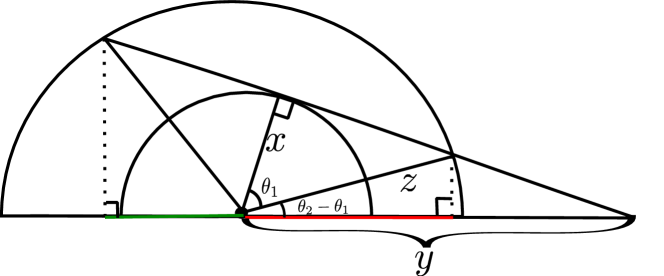
Proof A.2 (Proof of Lemma A.1)

For $d\geq 2$ and $x<z<y$, we follow the geometric approach which is adopted to derive $H(x)$ in [6]. Then we only need to compute the ratio of surface area on the sphere with radius $z$. This is the area between two planes at distance $\frac{a_{1}}{z}$ and $\frac{a_{2}}{z}$ respectively on the unit sphere. From (1.1) of [8], this ratio equals $\kappa(\frac{a_{2}}{z})-\kappa(\frac{a_{1}}{z})$ where $\kappa$ is defined in (6).

To show $K(x)=\int_{x}^{+\infty}\lambda_{d}(\frac{x}{y})|\mathrm{d}F(y)|$ in (9), we only need to connect $\lambda_{d}(r)$ with its geometric meaning, which is given in the following lemma:

Lemma A.3

The ratio of surface area on a unit $d$-sphere, satisfying $x_{1}^{2}+x_{2}^{2}\geq r$ is $\lambda_{d}(r)$, defined in (8).

Proof A.4

Following [8], we use $\kappa_{d}=2\pi^{d/2}/\Gamma(d/2)$ to represent the surface area of the unit $d$-sphere. Then

$\displaystyle\lambda_{d}(r)$ $\displaystyle=\frac{1}{\kappa_{d}}\cdot 2\int_{\begin{subarray}{c}x_{1}^{2}+x_{2}^{2}\geq r^{2}\\ x_{1}^{2}+\dots+x_{d-1}^{2}\leq 1\end{subarray}}\frac{1}{\sqrt{1-x_{1}^{2}-\dots-x_{d-1}^{2}}}\mathrm{d}x_{1}\dots\mathrm{d}x_{d-1}$
$\displaystyle=\frac{4\pi}{\kappa_{d}}\int_{r}^{1}x\mathrm{d}x\int_{x_{3}^{2}+\dots+x_{d-1}^{2}\leq 1-x^{2}}\frac{\mathrm{d}x_{3}\dots\mathrm{d}x_{d-1}}{\sqrt{1-x^{2}-x_{3}^{2}-\dots-x_{d-1}^{2}}}$
$\displaystyle=\frac{4\pi\kappa_{d-3}}{\kappa_{d}}\int_{r}^{1}x\mathrm{d}x\int_{0}^{\sqrt{1-x^{2}}}\frac{y^{d-4}\mathrm{d}y}{\sqrt{1-x^{2}-y^{2}}}$
$\displaystyle=\frac{4\pi\kappa_{d-3}}{\kappa_{d}}\int_{0}^{\sqrt{1-r^{2}}}y^{d-4}\mathrm{d}y\int_{r}^{\sqrt{1-y^{2}}}\frac{x\mathrm{d}x}{\sqrt{1-x^{2}-y^{2}}}$
$\displaystyle=\frac{4\pi\kappa_{d-3}}{\kappa_{d}}\int_{0}^{\sqrt{1-r^{2}}}y^{d-4}\sqrt{1-r^{2}-y^{2}}\mathrm{d}y$
$\displaystyle=\frac{4\pi\kappa_{d-3}}{\kappa_{d}}\frac{B(\frac{3}{2},\frac{d-3}{2})}{2}(1-r^{2})^{(d-2)/2}$
$\displaystyle=(1-r^{2})^{(d-2)/2}$
Lemma A.5

For $0<c<1$ and $n$ is a non-negative positive integer, we have

$$\int_{0}^{c}[\frac{1}{(1-t)^{n+1}}+\frac{1}{(1+t)^{n+1}}](c^{2}-t^{2})^{(n-1)/2}\mathrm{d}t=B(\frac{n+1}{2},\frac{1}{2})\frac{c^{n}}{(1-c^{2})^{(n+1)/2}}$$ (39)
Proof A.6 (Proof of Lemma A.5)

When $n=0$, the left hand side equals

$\displaystyle\int_{0}^{c}\frac{2}{(1-t^{2})\sqrt{c^{2}-t^{2}}}\mathrm{d}t=\int_{0}^{\sqrt{c}}\frac{1}{(1-t)\sqrt{t}\sqrt{c^{2}-t}}\mathrm{d}t$

We make change of variables $x=\sqrt{t/(c^{2}-t)}$ and obtain the value $\frac{\pi}{(1-c^{2})^{1/2}}$, which equals the right hand side. When $n=1$, we can use integration directly to show that (39) holds.

Let

$$h(n,c)=\int_{0}^{c}[\frac{1}{(1-t)^{n+1}}+\frac{1}{(1+t)^{n+1}}](c^{2}-t^{2})^{(n-1)/2}\mathrm{d}t$$ (40)

When $n\geq 2$, by integration by parts we have

$$\frac{n}{n-1}h(n,c)=\int_{0}^{c}\left[\frac{1}{(1-t)^{n}}-\frac{1}{(1+t)^{n}}\right]t(c^{2}-t^{2})^{(n-3)/2}\mathrm{d}t$$ (41)

Let $t=\frac{(1+t)-(1-t)}{2}$ in the right hand side of (41), then

$$2\frac{n}{n-1}h(n,c)=-h(n-2,c)+\int_{0}^{c}\left[\frac{1+t}{(1-t)^{n}}+\frac{1-t}{(1+t)^{n}}\right](c^{2}-t^{2})^{(n-3)/2}\mathrm{d}t$$ (42)

On the other hand, From (40), $(c^{2}-t^{2})^{(n-1)/2}=[(c^{2}-1)+(1-t^{2})](c^{2}-t^{2})^{(n-3)/2}$

$$h(n,c)=\frac{c^{2}-1}{2c}\frac{2}{n-1}\frac{\partial h(n,c)}{\partial c}+\int_{0}^{c}\left[\frac{1+t}{(1-t)^{n}}+\frac{1-t}{(1+t)^{n}}\right](c^{2}-t^{2})^{(n-3)/2}\mathrm{d}t$$ (43)

Therefore,

$$h(n,c)=\frac{c^{2}-1}{2c}\frac{2}{n-1}\frac{\partial h(n,c)}{\partial c}+[2\frac{n}{n-1}h(n,c)+h(n-2,c)]$$ (44)

then we can use induction and solve this first order linear ODE about $h(n,c)$. The initial condition is $h(n,0)=0$ and suppose $h(n-2,c)=B(\frac{n-1}{2},\frac{1}{2})\frac{c^{n-2}}{(1-c^{2})^{(n-1)/2}}$. Then (44) is simplified as

$$\frac{\partial h(n,c)}{\partial c}-\frac{(n+1)c}{1-c^{2}}h(n,c)=B(\frac{n-1}{2},\frac{1}{2})\frac{(n-1)c^{n-1}}{(1-c^{2})^{(n+1)/2}}$$ (45)

Using the integration factor $I(c)=(1-c^{2})^{(n+1)/2}$, we obtain

$$h(n,c)=B(\frac{n+1}{2},\frac{1}{2})\frac{c^{n}}{(1-c^{2})^{(n+1)/2}}$$ (46)

Having defined $K(x),F_{0}(x)$, we find the following relationship holds:

Lemma A.7
$$\int_{u}^{+\infty}(1-\frac{u^{2}}{x^{2}})^{\frac{d-3}{2}}|\mathrm{d}F_{0}(x)|=K^{2}(u)$$ (47)
Proof A.8 (Proof of Lemma A.7)

By the chain rule, from (38) we obtain

$\displaystyle\frac{\mathrm{d}}{\mathrm{d}x}\frac{a_{1}}{z}$ $\displaystyle=\sin(\theta_{2}-\theta_{1})\left(\frac{-1}{z\sin\theta_{1}}+\frac{1}{y\sin\theta_{2}}\right)$
$\displaystyle\frac{\mathrm{d}}{\mathrm{d}x}\frac{a_{2}}{z}$ $\displaystyle=\sin(\theta_{2}+\theta_{1})\left(\frac{1}{z\sin\theta_{1}}+\frac{1}{y\sin\theta_{2}}\right)$

where $\theta_{1},\theta_{2}$ are defined in (37). Then from (34)

$\displaystyle\frac{\mathrm{d}F_{0}(x)}{\mathrm{d}x}=\frac{2\Gamma(\frac{d}{2})}{\sqrt{\pi}\Gamma(\frac{d-1}{2})}\int_{x}^{+\infty}|\mathrm{d}F(y)|\int_{x}^{y}|f(x,y,z)||\mathrm{d}F(z)|$

where

$\displaystyle f(x,y,z)=\sin^{d-2}(\theta_{2}-\theta_{1})\left(\frac{-1}{z\sin\theta_{1}}+\frac{1}{y\sin\theta_{2}}\right)-\sin^{d-2}(\theta_{1}+\theta_{2})\left(\frac{1}{z\sin\theta_{1}}+\frac{1}{y\sin\theta_{2}}\right)$

Comparing $\mathrm{d}F_{0}(x)$ with the expression of $K(x)$ in (9), we only need to prove

$$\frac{2\Gamma(\frac{d}{2})}{\sqrt{\pi}\Gamma(\frac{d-1}{2})}\int_{u}^{z}(1-\frac{u^{2}}{x^{2}})^{\frac{d-3}{2}}|f(x,y,z)|\mathrm{d}x=2(1-\frac{u^{2}}{y^{2}})^{\frac{d-2}{2}}(1-\frac{u^{2}}{z^{2}})^{\frac{d-2}{2}}$$ (48)

We can expand $f(x,y,z)$ as follows:

$\displaystyle-f(x,y,z)$ $\displaystyle=\frac{\sin^{d-2}(\theta_{2}+\theta_{1})+\sin^{d-2}(\theta_{2}-\theta_{1})}{z\sin\theta_{1}}+\frac{\sin^{d-2}(\theta_{2}+\theta_{1})-\sin^{d-2}(\theta_{2}-\theta_{1})}{y\sin\theta_{2}}$
$\displaystyle=\frac{2}{z\sin\theta_{1}}\sum_{k\textrm{ is even}}\binom{d-2}{k}(\sin\theta_{2}\cos\theta_{1})^{d-2-k}(\cos\theta_{2}\sin\theta_{1})^{k}$
$\displaystyle+\frac{2}{y\sin\theta_{2}}\sum_{k\textrm{ is odd}}\binom{d-2}{k}(\sin\theta_{2}\cos\theta_{1})^{d-2-k}(\cos\theta_{2}\sin\theta_{1})^{k}$

Therefore,

$\displaystyle|f(x,y,z)|$ $\displaystyle=\frac{2x^{d-2}}{y^{d-2}z^{d-2}}\Big{[}\sum_{k\textrm{ is even}}\binom{d-2}{k}(z^{2}-x^{2})^{\frac{k-1}{2}}(y^{2}-x^{2})^{\frac{d-2-k}{2}}$
$\displaystyle+\sum_{k\textrm{ is odd}}\binom{d-2}{k}(z^{2}-x^{2})^{\frac{k}{2}}(y^{2}-x^{2})^{\frac{d-3-k}{2}}\Big{]}$

Let $a=z^{2}-u^{2},b=y^{2}-u^{2}$, then

$\displaystyle\int_{u}^{z}(1-\frac{u^{2}}{x^{2}})^{\frac{d-3}{2}}|f(x,y,z)|\mathrm{d}x=\frac{1}{y^{d-2}z^{d-2}}\int_{0}^{a}x^{\frac{d-3}{2}}\Big{[}$
$\displaystyle\sum_{k\textrm{ is even}}\binom{d-2}{k}(a-x)^{\frac{k-1}{2}}(b-x)^{\frac{d-2-k}{2}}+\sum_{k\textrm{ is odd}}\binom{d-2}{k}(a-x)^{\frac{k}{2}}(b-x)^{\frac{d-3-k}{2}}\Big{]}\mathrm{d}x$
$\displaystyle=\frac{1}{2y^{d-2}z^{d-2}}\int_{0}^{a}x^{\frac{d-3}{2}}\Big{[}\frac{(\sqrt{b-x}+\sqrt{a-x})^{d-2}+(\sqrt{b-x}-\sqrt{a-x})^{d-2}}{\sqrt{a-x}}$
$\displaystyle+\frac{(\sqrt{b-x}+\sqrt{a-x})^{d-2}-(\sqrt{b-x}-\sqrt{a-x})^{d-2}}{\sqrt{b-x}}\Big{]}\mathrm{d}x$

Let $t=\sqrt{\frac{a-x}{b-x}}$, we then obtain

$\displaystyle\int_{u}^{z}(1-\frac{u^{2}}{x^{2}})^{\frac{d-3}{2}}|f(x,y,z)|\mathrm{d}x$
$\displaystyle=\frac{(b-a)^{\frac{d-1}{2}}}{y^{d-2}z^{d-2}}\int_{0}^{\sqrt{a/b}}\left[\frac{1}{(1-t)^{d-1}}+\frac{1}{(1+t)^{d-1}}\right](a-bt^{2})^{\frac{d-3}{2}}\mathrm{d}t$

Let $c=\sqrt{a/b}$ and $n=d-2\geq 0$ in the expression of $h(n,c)$ in (46), we obtain

$\displaystyle\int_{u}^{z}(1-\frac{u^{2}}{x^{2}})^{\frac{d-3}{2}}|f(x,y,z)|\mathrm{d}x=\frac{1}{y^{d-2}z^{d-2}}h(d-2,\sqrt{a/b})(1-c^{2})^{\frac{n+1}{2}}b^{\frac{n}{2}}$ (49)

After simplification of (49), we obtain (48).

Proof A.9 (Proof of Theorem 3.1)

We use $\operatorname{dist}(P_{1},\dots,P_{d-1})$ to represent the distance from the origin to the hyperplane passing $P_{1},P_{2},\dots,P_{d-1}$, and let $F_{1}(x)=P(\operatorname{dist}(P_{1},\dots,P_{d-1})\linebreak\geq x)$.

Firstly we show that $F_{1}(x)=K^{d-1}(x)$. For $d=2$, it is trivial. By induction we suppose that $F_{1}(x)=K^{d^{\prime}-1}(x)$ is true for $d^{\prime}\leq d-1$. Since $d^{\prime}\leq d$, the function $K(x)=P(\sqrt{(X^{(1)})^{2}+(X^{(2)})^{2}}\geq x)$ only depends on $d$, not on $d^{\prime}$. Therefore, in $d^{\prime}$-dimensional space, from (9) we have $P(\operatorname{dist}(P_{1},\dots,P_{d^{\prime}-1})\geq x)=\int_{x}^{\infty}K^{d^{\prime}-2}(x)\lambda_{d^{\prime}}(x/y)|\mathrm{d}F(y)|$. Then the conditional probability $P(\operatorname{dist}(P_{1},\dots,P_{d^{\prime}-1})\geq x\Big{|}|OP_{1}|=y)=K^{d^{\prime}-2}(x)\lambda_{d^{\prime}}(x/y)$. For $d$-dimensional space, we firstly specify a straight line passing through $P_{d-2}P_{d-1}$, the space perpendicular to this line has $d^{\prime}=d-1$ dimension while the straight line shrinks to a single point $P^{\prime}$ in this subspace. Since $P(\operatorname{dist}(P_{1},\dots,P_{d-3},P^{\prime})\geq x\Big{|}|OP^{\prime}|=y)=K^{d-3}(x)\lambda_{d-1}(x/y)$, we have

$\displaystyle F_{1}(x)=\int_{x}^{+\infty}K^{d-3}(x)\lambda_{d-1}(\frac{x}{y})|\mathrm{d}F_{0}(y)|$

From Lemma A.7 we obtain $F_{1}(x)=K^{d-1}(x)$.

To finish the proof and compute $H(x)$, we first specify a hyperplane $P_{2}P_{3}\dots P_{d}$, whose distance to the origin is $y$. The subspace perpendicular to this hyperplane is a 2-D subspace, and this hyperplane shrinks to a point $P^{\prime}$ in this 2-D subspace. Similar to (1.9) of [6], we have

$\displaystyle H(x)$ $\displaystyle=\frac{2}{\pi}\int_{x}^{+\infty}|\mathrm{d}F_{1}(y)|\left[\int_{x}^{y}\arccos\frac{x}{z}|\mathrm{d}K(z)|+\int_{y}^{+\infty}\arccos\frac{x}{y}|\mathrm{d}K(z)|\right]$ (50)
$\displaystyle=\frac{2}{\pi}\int_{x}^{+\infty}\arccos\frac{x}{z}F_{1}(z)|\mathrm{d}K(z)|+\frac{2}{\pi}\int_{x}^{+\infty}K(y)F_{1}(y)\arccos\frac{x}{y}|\mathrm{d}F_{1}(y)|$

Using $F_{1}(x)=K^{d-1}(x)$, we reduce (50) to

$$H(x)=\frac{2}{\pi}\int_{x}^{+\infty}\arccos\frac{x}{y}\cdot d\cdot K^{d-1}(y)|\mathrm{d}K(y)|$$

which is exactly (7).

Appendix B Computations involved in three distribution tails

B.1 Computations involved in polynomial tails

The techniques used in this subsection are similar to the derivation of $G(x)$ in (2.3) of [6].

Proof B.1 (Proof of Theorem 4.2)

For polynomial tails defined in (13), we first compute the asymptotic value of $K(x)$ as follows:

$\displaystyle K(x)$ $\displaystyle=\int_{x}^{\infty}(1-\frac{x^{2}}{y^{2}})^{\frac{d-2}{2}}|\mathrm{d}F(y)|$
$\displaystyle=(d-2)\int_{x}^{\infty}F(y)\frac{x^{2}}{y^{3}}(1-\frac{x^{2}}{y^{2}})^{\frac{d-4}{2}}\mathrm{d}y$
$\displaystyle(y=x/t)$ $\displaystyle=(d-2)x^{-k}\int_{0}^{1}L(x/t)t^{k+1}(1-t^{2})^{(d-4)/2}\mathrm{d}t$
$\displaystyle\sim F(x)\frac{d-2}{2}B\left(\frac{k+2}{2},\frac{d}{2}-1\right)$

Then applying Theorem 3.1, we obtain

$\displaystyle H(x)$ $\displaystyle=\frac{2}{\pi}\int_{x}^{\infty}\arccos\frac{x}{y}|\mathrm{d}K^{d}(y)|$
$\displaystyle\sim\frac{2}{\pi}\left(\frac{d-2}{2}\right)^{d}B^{d}\left(\frac{k+2}{2},\frac{d}{2}-1\right)\int_{x}^{\infty}\frac{x}{y\sqrt{y^{2}-x^{2}}}F^{d}(y)\mathrm{d}y$
$\displaystyle\sim\frac{2}{\pi}\left(\frac{d-2}{2}\right)^{d}B^{d}\left(\frac{k+2}{2},\frac{d}{2}-1\right)\frac{1}{2}B\left(\frac{1}{2},\frac{dk+1}{2}\right)L^{d}(x)x^{-dk}$
$\displaystyle\sim\frac{2^{d}\pi^{(d-1)/2}\Gamma^{d}(\frac{k}{2}+1)\Gamma(\frac{dk+1}{2})}{\Gamma^{d}(\frac{k+1}{2})\Gamma(\frac{dk}{2}+1)}G(x)^{d}$

To simplify the notation, we denote $g(d)=\frac{2^{d}\pi^{(d-1)/2}\Gamma^{d}(\frac{k}{2}+1)\Gamma(\frac{dk+1}{2})}{\Gamma^{d}(\frac{k+1}{2})\Gamma(\frac{dk}{2}+1)}$. Let $G(x)=w$, then from (10)

$\displaystyle\mathbb{E}[F_{N}]$ $\displaystyle\sim g(d)\binom{N}{d}\int_{0}^{+\infty}(1-w)^{N-d}|\mathrm{d}w^{d}|$
$\displaystyle\sim g(d)\binom{N}{d}d\int_{0}^{1/2}\exp(-(N-d)w)w^{d-1}\mathrm{d}w$
$\displaystyle\sim\frac{N!}{(N-d)!(N-d)^{d}}g(d)$ (51)

And (16) is obtained from (51).

The following part in this subsection discusses how to derive (20). We first give two lemmas, which are useful to handle the case when $d\to\infty$.

Lemma B.2

For fixed $v>0$, we have

$$\frac{\Gamma(n+v)}{\Gamma(n)}\sim n^{v}\textrm{ as }n\to\infty$$ (52)
Proof B.3

We use Beta function to prove (52). (52) is equivalent to $B(n,v)\sim\Gamma(v)n^{-v}$. From the definition of beta function, we have

$\displaystyle B(n,v)$ $\displaystyle=\int_{0}^{1}(1-x)^{n-1}x^{v-1}\mathrm{d}x$
$\displaystyle\sim\int_{0}^{\epsilon}\exp(-nx)x^{v-1}\mathrm{d}x\textrm{ for given }\epsilon>0$
$\displaystyle\sim n^{-v}\int_{0}^{n\epsilon}\exp(-x)x^{v-1}\mathrm{d}x$
$\displaystyle\sim\Gamma(v)n^{-v}$

We can use Stirling’s formula to prove that

Lemma B.4
$$\frac{N!}{(N-d)!(N-d)^{d}}\sim 1$$ (53)

when $N/d^{2}\to\infty$.

Proof B.5
$\displaystyle\frac{N!}{(N-d)!(N-d)^{d}}$ $\displaystyle\sim\sqrt{\frac{N}{N-d}}\frac{N^{N}}{e^{d}(N-d)^{N}}$
$\displaystyle\sim e^{-d}(1+\frac{d}{N-d})^{N}$
$\displaystyle\sim e^{-d}\exp(\frac{Nd}{N-d})$
$\displaystyle\sim\exp(\frac{d^{2}}{N-d})$

From the condition $N/d^{2}\to\infty$, we obtain (53).

Combining (52) with (53), we obtain (20) from (51).

B.2 Computations involved in exponential tails

Proof B.6 (Proof of Theorem 4.4)

For exponential tails, following Carnal [6], we make the substitution x=L​(s),y=L​(Οƒ)formulae-sequenceπ‘₯πΏπ‘ π‘¦πΏπœŽx=L(s),y=L(\sigma), then $\sigma=1/F(y)$. Substituting them into (9), we have

$\displaystyle K(x)$ $\displaystyle=\int_{s}^{\infty}\left(1-\frac{L(s)^{2}}{L(\sigma)^{2}}\right)^{\frac{d-2}{2}}\frac{\mathrm{d}\sigma}{\sigma^{2}}$

As $x\to\infty$, sβ†’βˆžβ†’π‘ s\to\infty, then L​(s)/L​(Οƒ)β†’1β†’πΏπ‘ πΏπœŽ1L(s)/L(\sigma)\to 1 for Οƒ<A​sπœŽπ΄π‘ \sigma<As, where $A$ is an arbitrary constant.

$\displaystyle K(x)$ ∼2dβˆ’22β€‹βˆ«sA​s(1βˆ’L​(s)L​(Οƒ))dβˆ’22​d​σσ2similar-toabsentsuperscript2𝑑22superscriptsubscript𝑠𝐴𝑠superscript1πΏπ‘ πΏπœŽπ‘‘22d𝜎superscript𝜎2\displaystyle\sim 2^{\frac{d-2}{2}}\int_{s}^{As}\left(1-\frac{L(s)}{L(\sigma)}\right)^{\frac{d-2}{2}}\frac{\mathrm{d}\sigma}{\sigma^{2}}
(3.6) of [8] ∼2dβˆ’22β€‹βˆ«sA​s(ϡ​(s)​log⁑σs)dβˆ’22​d​σσ2similar-toabsentsuperscript2𝑑22superscriptsubscript𝑠𝐴𝑠superscriptitalic-Ο΅π‘ πœŽπ‘ π‘‘22d𝜎superscript𝜎2\displaystyle\sim 2^{\frac{d-2}{2}}\int_{s}^{As}(\epsilon(s)\log\frac{\sigma}{s})^{\frac{d-2}{2}}\frac{\mathrm{d}\sigma}{\sigma^{2}}
$\displaystyle\sim 2^{\frac{d-2}{2}}\epsilon(s)^{\frac{d}{2}-1}\frac{1}{s}\int_{1}^{A}(\log x)^{\frac{d-2}{2}}\frac{\mathrm{d}x}{x^{2}}$
$\displaystyle\sim 2^{\frac{d}{2}-1}\Gamma\left(\frac{d}{2}\right)F(x)v(x)^{\frac{d}{2}-1}$

Similar techniques can be applied to compute the asymptotic value of $H(x)$.

$\displaystyle H(x)$ $\displaystyle=\frac{2}{\pi}\int_{x}^{+\infty}\frac{xK^{d}(y)}{y^{2}\sqrt{1-\frac{x^{2}}{y^{2}}}}\mathrm{d}y$
$\displaystyle=\frac{2}{\pi}\left[2^{\frac{d}{2}-1}\Gamma\left(\frac{d}{2}\right)\right]^{d}\int_{s}^{+\infty}\frac{L(s)\epsilon^{1+\frac{d(d-2)}{2}}(\sigma)}{L(\sigma)\sqrt{1-\frac{L^{2}(s)}{L^{2}(\sigma)}}\sigma^{d+1}}\mathrm{d}\sigma\textrm{ since }\mathrm{d}y=L(\sigma)\frac{\epsilon(\sigma)}{\sigma}\mathrm{d}\sigma$
∼2π​[2d2βˆ’1​Γ​(d2)]d​ϡd​(dβˆ’2)+12​(s)β€‹βˆ«s+∞(log⁑σs)βˆ’12β€‹Οƒβˆ’(d+1)​dΟƒsimilar-toabsent2πœ‹superscriptdelimited-[]superscript2𝑑21Γ𝑑2𝑑superscriptitalic-ϡ𝑑𝑑212𝑠superscriptsubscript𝑠superscriptπœŽπ‘ 12superscriptπœŽπ‘‘1differential-d𝜎\displaystyle\sim\frac{\sqrt{2}}{\pi}\left[2^{\frac{d}{2}-1}\Gamma\left(\frac{d}{2}\right)\right]^{d}\epsilon^{\frac{d(d-2)+1}{2}}(s)\int_{s}^{+\infty}\left(\log\frac{\sigma}{s}\right)^{-\frac{1}{2}}\sigma^{-(d+1)}\mathrm{d}\sigma
$\displaystyle=\frac{\sqrt{2}}{\sqrt{\pi d}}\left[2^{\frac{d}{2}-1}\Gamma\left(\frac{d}{2}\right)\right]^{d}\epsilon^{\frac{d(d-2)+1}{2}}(s)s^{-d}$
$\displaystyle=\frac{2^{\frac{d(d-2)+1}{2}}}{\sqrt{\pi d}}\Gamma^{d}\left(\frac{d}{2}\right)v^{\frac{d(d-2)+1}{2}}(x)F^{d}(x)$

From (23), we obtain (24).

Dwyer [8] has shown that for exponential tails, $v(x)\sim\epsilon(1/G(x))$ as $x\to\infty$. From (10), we use the Abel-Tauber theorem [12] and obtain

$\displaystyle\mathbb{E}[F_{N}]$ $\displaystyle\sim\frac{\pi^{\frac{d-1}{2}}2^{\frac{d+1}{2}}}{\sqrt{d}}\int_{0}^{1/2}\exp(-(N-d)w)\mathrm{d}[w^{d}\epsilon(1/w)^{\frac{-d+1}{2}}]$
$\displaystyle\sim\frac{\pi^{\frac{d-1}{2}}2^{\frac{d+1}{2}}}{\sqrt{d}}\binom{N}{d}\frac{\Gamma(d+1)}{(N-d)^{d}}\epsilon(N-d)^{\frac{-d+1}{2}}$

To obtain $\mathbb{E}[F_{N}]$ when $d\to\infty$, we need the following lemma.

Lemma B.7

Suppose $\epsilon(x)$ is a slowly varying function and $N(d)\gg d^{2}$, then $\epsilon(N-d)^{d}\sim\epsilon(N)^{d}$.

Proof B.8

Since $\epsilon(x)$ is slowly varying, there exists a bounded function $u(x)$ such that $\epsilon(y)/\epsilon(x)=\exp(\int_{x}^{y}\frac{u(t)}{t}\mathrm{d}t)$. Besides, $\lim_{x\to\infty}u(x)=0$. By the mean value theorem, there exists $\xi\in[x,y]$ such that $\epsilon(y)/\epsilon(x)=\exp(u(\xi)\int_{x}^{y}\frac{1}{t}\mathrm{d}t)=\exp(u(\xi)\log(y/x))$. Let $x=N-d,y=N$, and we obtain

$$\frac{\epsilon(N)^{d}}{\epsilon(N-d)^{d}}=\exp\left(u(\xi)\log\left(\frac{N}{N-d}\right)d\right)$$

As $N-d\to\infty$, $u(\xi)\to 0$. In addition, $\log(\frac{N}{N-d})\sim\frac{d}{N-d}\sim\frac{d}{N}$. Therefore, $\frac{\epsilon(N)^{d}}{\epsilon(N-d)^{d}}\sim\exp(\frac{u(\xi)d^{2}}{N})$. Since $N/d^{2}\to\infty,\frac{u(\xi)d^{2}}{N}\to 0$ and $\frac{\epsilon(N)^{d}}{\epsilon(N-d)^{d}}\to 1$.

By Lemma B.7, we can show that $\epsilon(N-d)^{\frac{-d+1}{2}}\sim\epsilon(N)^{\frac{-d+1}{2}}$. When $d\to\infty$ and $N/d^{2}\to\infty$, we further obtain (26).

B.3 Computations involved in truncated tails

Proof B.9 (Proof of Theorem 4.5)

First we compute $K(x)$ as follows

$\displaystyle K(1-x)$ $\displaystyle=\int_{1-x}^{1}\left(1-\frac{(1-x)^{2}}{y^{2}}\right)^{\frac{d-2}{2}}|\mathrm{d}F(y)|$
$\displaystyle\sim 2^{\frac{d-2}{2}}\int_{1-x}^{1}(y-1+x)^{\frac{d-2}{2}}|\mathrm{d}F(y)|$
$\displaystyle\sim 2^{\frac{d-2}{2}}\int_{0}^{x}(x-y)^{\frac{d-2}{2}}|\mathrm{d}F(1-y)|$
$\displaystyle\sim 2^{\frac{d-2}{2}}\frac{d-2}{2}\int_{0}^{x}y^{k}L(1/y)(x-y)^{\frac{d-4}{2}}\mathrm{d}y$
$\displaystyle\sim(d-2)2^{\frac{d}{2}-2}B(k+1,\frac{d}{2}-1)x^{k+\frac{d}{2}-1}L(1/x)$
$\displaystyle=k2^{\frac{d}{2}-1}B(k,\frac{d}{2})x^{k+\frac{d}{2}-1}L(1/x)$

Then using $\arccos x\sim\sqrt{2(1-x)}$ as $x\to 0^{+}$, we have

$\displaystyle H(1-x)$ $\displaystyle=\frac{2}{\pi}\int_{1-x}^{1}\arccos\frac{1-x}{y}|\mathrm{d}K^{d}(y)|$
$\displaystyle\sim\frac{2}{\pi}\int_{0}^{x}\sqrt{2}\sqrt{x-y}|\mathrm{d}K^{d}(1-y)|$
$\displaystyle\sim\frac{\sqrt{2}}{\pi}k^{d}2^{d(\frac{d}{2}-1)}B^{d}(k,\frac{d}{2})\int_{0}^{x}\frac{1}{\sqrt{x-y}}y^{d(k+\frac{d}{2}-1)}L^{d}(1/y)\mathrm{d}y$
$\displaystyle\sim\frac{k^{d}}{\pi}2^{\frac{1}{2}+d(\frac{d}{2}-1)}B^{d}(k,\frac{d}{2})B\left(\frac{1}{2},d(k+\frac{d}{2}-1)+1\right)L^{d}(1/x)x^{d(k+\frac{d}{2}-1)+\frac{1}{2}}$

which is (30).

From (28) and (30), it follows that

$$H(1-x)\sim ba^{-d}G(1-x)^{d}x^{\frac{1-d}{2}}$$ (54)

Let $G(1-x)=w$, similar to the analysis in (2.7) of [6], we obtain

$$x\sim[\frac{w}{a}L(w^{-1})]^{\frac{2}{2k+d-1}}\textrm{ as }w\to 0$$

Finally, we apply the Abel-Tauber theorem [12], and from (10) we obtain

$\displaystyle\mathbb{E}[F_{N}]$ $\displaystyle=\binom{N}{d}\int_{0}^{1}(1-G(1-x))^{N-d}|\mathrm{d}H(1-x)|$
$\displaystyle\sim\binom{N}{d}\frac{b}{a^{d}}\int_{0}^{1/2}\exp(-(N-d)w)\mathrm{d}[w^{d}(\frac{w}{a}L(w^{-1}))^{\frac{1-d}{2k+d-1}}]$
$\displaystyle\sim\frac{\binom{N}{d}}{(N-d)^{d}}ba^{-d+\frac{d-1}{2k+d-1}}\Gamma\left(d+1-\frac{d-1}{2k+d-1}\right)(N-d)^{\frac{d-1}{2k+d-1}}L(N-d)^{\frac{d-1}{2k+d-1}}$ (55)

When $N\to\infty$ and $d$ is a constant, we obtain (32).

The asymptotic value of $\mathbb{E}[F_{N}]$ when $d\to\infty$ is derived as follows:

From (29) and (31), it follows that

$$ba^{-d}=\frac{\pi^{(d-1)/2}2^{(d+1)/2}\Gamma^{d}(k+\frac{d+1}{2})\Gamma(d(k+\frac{d}{2}-1)+1)}{\Gamma^{d}(k+\frac{d}{2})\Gamma(d(k+\frac{d}{2}-1)+\frac{3}{2})}$$ (56)

When $d\to\infty$, using Lemma B.2, we obtain the asymptotic value of $ba^{-d}$ as

$$ba^{-d}\sim 2\pi^{(d-1)/2}d^{-1}e^{k}d^{d/2}$$ (57)

From (29), the asymptotic value of $a$ is given as

$$a\sim\pi^{-1/2}2^{\frac{d-2+2k}{2}}k\Gamma(k)d^{-k-\frac{1}{2}}$$ (58)

When $d\to\infty$ and $N/d^{2}\to\infty$, from (55) we have $\mathbb{E}[F_{N}]\sim ba^{-d}aN^{\frac{d-1}{2k+d-1}}L(N)^{\frac{d-1}{2k+d-1}}$. Then by a slight simplification, (33) is obtained.

\fund

This research was funded in part by the Shenzhen Science and Technology Program under Grant KQTD20170810150821146, National Key R&D Program of China under Grant 2021YFA0715202 and High-end Foreign Expert Talent Introduction Plan under Grant G2021032013L.

\competing

There were no competing interests to declare which arose during the preparation or publication process of this article.

References

  • [1] Affentranger, F. (1991). The convex hull of random points with spherically symmetric distributions. Rend. Sem. Mat. Univ. Politec. Torino 49, 359–383.
  • [2] Aldous, D.Β J., Fristedt, B., Griffin, P.Β S. and Pruitt, W.Β E. (1991). The number of extreme points in the convex hull of a random sample. Journal of applied probability 28, 287–304.
  • [3] Balestriero, R., Pesenti, J. and LeCun, Y. (2021). Learning in high dimension always amounts to extrapolation. arXiv preprint arXiv:2110.09485.
  • [4] BΓ‘rΓ‘ny, I. (2008). Random points and lattice points in convex bodies. Bulletin of the American Mathematical Society 45, 339–365.
  • [5] Brondsted, A. (2012). An introduction to convex polytopes vol.Β 90. Springer Science & Business Media.
  • [6] Carnal, H. (1970). Die konvexe hΓΌlle von n rotationssymmetrisch verteilten punkten. Zeitschrift fΓΌr Wahrscheinlichkeitstheorie und verwandte Gebiete 15, 168–176.
  • [7] Davis, R., Mulrow, E. and Resnick, S. (1987). The convex hull of a random sample in $\mathbb{R}^{2}$. Stochastic Models 3, 1–27.
  • [8] Dwyer, R.Β A. (1991). Convex hulls of samples from spherically symmetric distributions. Discrete applied mathematics 31, 113–132.
  • [9] Efron, B. (1965). The convex hull of a random set of points. Biometrika 52, 331–343.
  • [10] Hueter, I. (1999). Limit theorems for the convex hull of random points in higher dimensions. Transactions of the American Mathematical Society 351, 4337–4363.
  • [11] Kabluchko, Z. and Zaporozhets, D. (2020). Absorption probabilities for gaussian polytopes and regular spherical simplices. Advances in Applied Probability 52, 588–616.
  • [12] Omey, E. and Willekens, E. (1989). Abelian and tauberian theorems for the laplace transform of functions in several variables. Journal of multivariate analysis 30, 292–306.
  • [13] Raynaud, H. (1970). Sur l’enveloppe convexe des nuages de points alΓ©atoires dans rn. i. Journal of Applied Probability 7, 35–48.
  • [14] RΓ©nyi, A. and Sulanke, R. (1963). Über die konvexe hΓΌlle von n zufΓ€llig gewΓ€hlten punkten. Zeitschrift fΓΌr Wahrscheinlichkeitstheorie und verwandte Gebiete 2, 75–84.
  • [15] Schneider, R. and Weil, W. (2008). Stochastic and integral geometry vol.Β 1. Springer. ch.Β 8.2.
  • [16] Seidel, R. (1997). Convex Hull Computations. CRC Press, Inc., USA. p.Β 361–375.
  • [17] Soms, A.Β P. (1976). An asymptotic expansion for the tail area of the t-distribution. Journal of the American Statistical Association 71, 728–730.