Gravitational memory effects of black bounces and a traversable wormhole

Abstract

Black bounces are spacetimes that can be interpreted as either black holes or wormholes depending on specific parameters. In this study, we examine the Simpson-Visser and Bardeen-type solutions as black bounces and investigate the gravitational wave in the background of these solutions. We then explore the displacement and velocity memory effects by analyzing the deviation of two neighboring geodesics and their derivatives influenced by the magnetic charge parameter $a$. This investigation aims to trace the magnetic charge in the gravitational memory effect. Additionally, we consider another family of traversable wormhole solutions obtained from non-exotic matter sources to trace the electric charge $Q_{e}$ in the gravitational memory effect, which can be determined from the far field asymptotic. This project is significant not only for detecting the presence of compact objects like wormholes through gravitational memory effects but also for observing the charge $Q_{e}$, which provides a concrete realization of Wheeler’s concept of ”electric charge without charge.”

I Introduction

General relativity (GR) is widely acknowledged as the most suitable and comprehensive theory for elucidating the gravitational interaction a1 ; a2 . This theory has exhibited remarkable success in addressing numerous quandaries and possesses the capacity to predict novel phenomena a3 ; a4 ; a5 ; a6 ; a7 ; a8 ; a9 ; 10 . Notably, the equations formulated by Einstein yield intriguing solutions, such as the Schwarzschild black hole. This particular black hole is distinguished by its static and symmetrical nature, devoid of both spin and charge 11 . Furthermore, general relativity presents solutions known as wormholes, which establish connections between disparate points in space-time within the same universe or even across different universes via a tunnel 13 . The characteristics of these wormhole solutions, including their traversability, resemblance to black holes, and stability, have been extensively investigated in various scholarly sources 14 ; 15 ; 16 ; 17 ; 18 ; 19 ; 20 ; 21 ; 22 ; 23 ; 24 ; 25 ; 26 ; 27 ; 28 ; 29 ; 30 ; 31 ; 32 ; 33 ; 34 ; 35 ; 36 ; 37 .

Furthermore, Einstein equations have been shown to have solutions for black holes and wormholes through the use of a nonlinear electromagnetic source. Additionally, a distinct type of solution known as regular black holes has been discovered, which possess an event horizon but lack a singularity. The original proposal for this solution was made by BardeenBardeen . One notable feature of regular black holes is the deviation of photons from geodesics, as well as changes in the thermodynamics of these solutions 40 ; 41 ; 42 . For more information on this solution, please refer to 43 ; 44 ; 45 ; 46 ; 47 ; 48 ; 49 ; 50 ; 51 ; 52 ; 53 ; 54 ; 55 .

The black bounce, a novel variant of a regular solution, has the unique ability to transform into either a black hole or a wormhole, depending on the specific parameters chosen. One of the most notable examples of this intriguing solution is the Simpson-Visser black bounce SV , which features a throat located at $r=0$ and an event horizon area that remains unaffected by the solution’s parameters. For alternative models of black holes, references 57 ; 58 ; 59 ; 60 may be consulted. Extensive investigations have been conducted on various properties of these models, without explicitly attributing them to the source of matter 61 ; 62 ; 63 ; 64 ; 65 ; 66 ; 67 ; 68 ; 69 ; 70 ; 71 ; 72 ; 73 ; 74 ; 75 ; 76 ; 77 ; 78 ; 79 . However, it is important to note that nonlinear electromagnetic fields alone are insufficient in describing the matter source responsible for the existence of the black bounce in the context of GR. To identify a suitable source for this solution, the inclusion of scalar and phantom fields becomes necessary, as discussed in main .

One of the challenges in constructing traversable wormholes is the requirement of exotic matter. To circumvent this problem, some alternative approaches based on generalized theories of gravity have been investigated. Among these, higher-curvature theories of gravity provide a promising framework for the existence of stable wormholes. A notable example is the low-energy heterotic string effective theory b7b7 ; b8b8 , which generalizes the four-dimensional gravitational theory by adding extra fields and higher-curvature terms to the standard Einstein-Hilbert action. Within this scenario, some studies have explored the possibility of traversable wormholes without the need for any exotic matter, using the dilatonic Einstein-Gauss-Bonnet theory in four-dimensional spacetime a7a7 . Moreover, recent research has attempted to construct a traversable wormhole solution by employing fermions and linear electromagnetic fields as the source terms prl .

This paper investigates the black bounce solutions and traversable wormholes in the context of gravitational memory effects, using fermions and linear electromagnetic fields as the source terms. The gravitational memory effect refers to the imprint of gravitational waves (GW) on the background metric that satisfies Einstein’s equations. This phenomenon, which was discovered long ago m1 ; m2 ; m3 ; m4 , originates from the propagation of energy flux to the future null infinity, where the spacetime becomes asymptotically flat x1 . The region where this effect takes place is governed by an asymptotic symmetry group called the Bondi-Metzner-Sachs (BMS) group bondii ; bondi1 ; bondi2 . The study of the infrared structure of gravity is of great importance for physicists, and the memory effect is one of the key features of interest infrared1 ; infrared2 ; infrared3 .

The detection of GWs, as reported in GW1 ; GW2 ; GW3 ; GW4 ; GW5 ; GW6 ; GW7 ; GW8 , reveals another intriguing aspect of the gravitational memory effect. This is the topic that we will concentrate on in this paper. We will investigate the gravitational memory effects by measuring the deviation of two nearby geodesics in this solution due to a GW pulse. We will examine the Simpson-Visser and Bardeen-Type black bounce solutions and a traversable wormhole solution in the presence of fermions and linear electromagnetic fields as the source terms under the influence of a GW pulse, in order to find the signatures of these compact objects in the deviation of two nearby geodesics as memory effects. The parameters of these solutions determine their impact on the deviation of two nearby geodesics. We will study the geodesic memory effect for the Simpson-Visser solution and the Bardeen-Type black bounce solution in sections II and III, respectively. In section IV, we will discuss the characteristics of the traversable wormhole solution by fermions and linear electromagnetic fields as the source terms and their implications for the memory effects. Finally, we will present our conclusions in section V.

II Geodesic memory effect for Simpson-Visser solution as a black bounce

Within this section, we explore the geodesic memory effect by examining the deviation of geodesics between neighboring points. This deviation arises due to the propagation of a GW, with the separation of geodesics measuring the extent of the displacement memory effect. Furthermore, we also investigate the velocity memory effect that occurs following the passage of a GW pulse. Hence, in this particular model, we have a black bounce solution serving as the background, with the GW pulse being introduced to this backdrop.

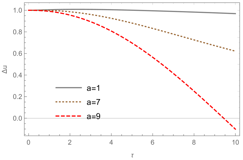
Figure 1: Variation of $\Delta u$ due to GW pulse has been presented with respect to $\tau$, for different choices of $a$ for Simpson-Visser black bounce.

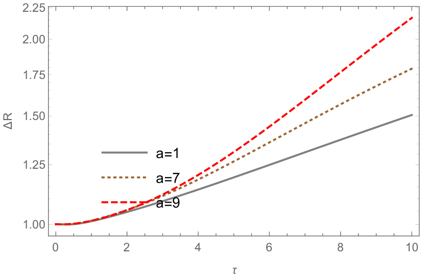
Figure 2: Variation of $\Delta R$ due to GW pulse with respect to $\tau$, for different choices of $a$ for Simpson-Visser black bounce.

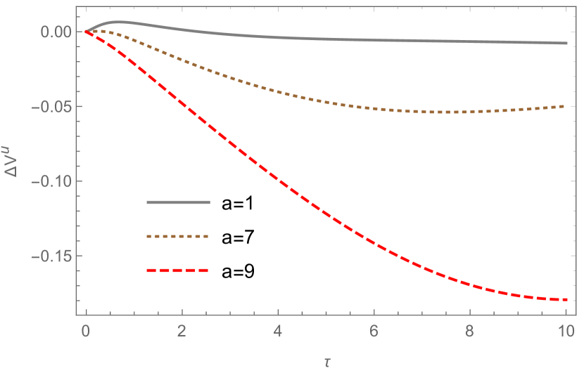
Figure 3: Variation of $\Delta V^{u}$ due to GW pulse with respect to $\tau$, for different choices of $a$ for Simpson-Visser black bounce.

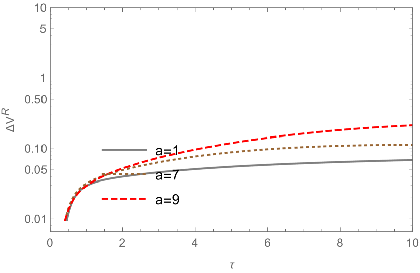
Figure 4: Variation of $\Delta V^{R}$ due to GW pulse with respect to $\tau$, for different choices of $a$ for Simpson-Visser black bounce.

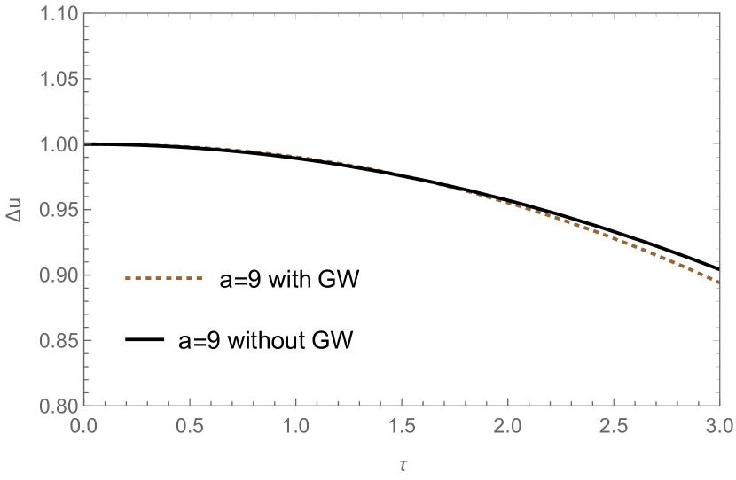
Figure 5: Variation of $\Delta u$ due to GW pulse and without GW pulse with respect to $\tau$ of Simpson-Visser black bounce.

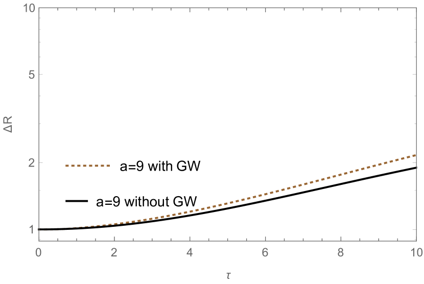
Figure 6: Variation of $\Delta R$ due to GW pulse and without GW pulse with respect to $\tau$ of Simpson-Visser black bounce.

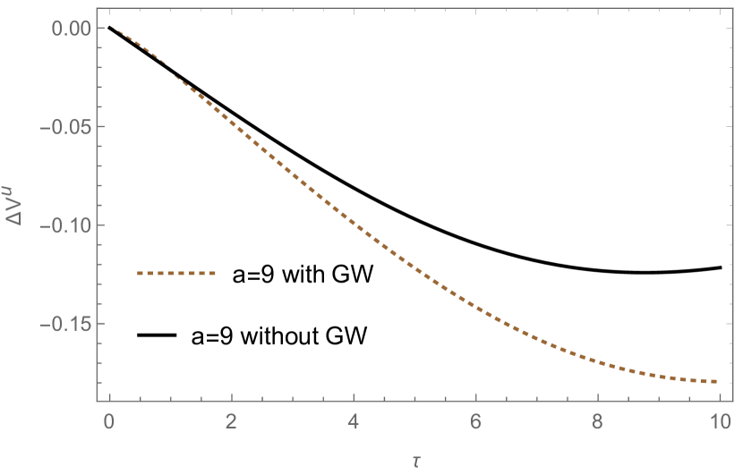
Figure 7: Variation of $\Delta V^{u}$ due to GW pulse and without GW pulse with respect to $\tau$ of Simpson-Visser black bounce.

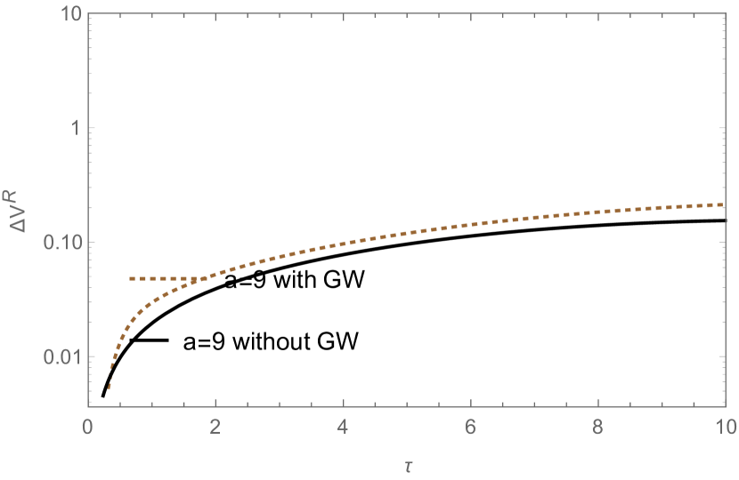
Figure 8: Variation of $\Delta V^{R}$ due to GW pulse and without GW pulse with respect to $\tau$ of Simpson-Visser black bounce.

Recent studies 1 ; 2 ; 3 ; 4 ; 5 have examined these phenomena by analyzing the trajectory of geodesics in precise plane GW spacetimes. To achieve this, a Gaussian pulse is selected to represent the polarization in the metric of the plane GW spacetime. Subsequently, the geodesic equations are solved using numerical methods, allowing for the calculation of the displacement and velocity memory effects, which correspond to the changes in separation and velocity, respectively. Additionally, alternative theories of gravity have been explored within this framework 6 ; 7 .

In this study, we investigate the development of geodesics within the black bounce background while considering the influence of a GW pulse. We demonstrate the relationship between the displacement and memory effects and their dependence on this particular background. The line element that describes a black bounce can be expressed as the general solution.

$$ds^{2}=-f(r)dt^{2}+f(r)^{-1}dr^{2}+\sigma(r)^{2}(d\theta^{2}+\sin^{2}\theta d\phi^{2})$$ (1)

If we constrain the solution to Simpson-Visser black bounce then we have

$$f(r)=1-\frac{2m}{\sqrt{r^{2}+a^{2}}}~{}~{}~{}and~{}~{}~{}\sigma(r)=\sqrt{r^{2}+a^{2}}$$ (2)

The magnetic charge, denoted by the parameter $a$, assumes a significant role in averting the emergence of a singularity at $r=0$. This fact can be substantiated through the computation of the Kretschmann scalar, a scalar invariant that quantifies the curvature of spacetime. The expression for the Kretschmann scalar corresponding to this particular solution is provided as follows.

$$R_{\mu\nu\rho\sigma}R^{\mu\nu\rho\sigma}=\frac{m^{2}\left(36a^{4}-48a^{2}r^{2}+47r^{4}\right)+32ma^{2}\left(r^{2}-a^{2}\right)\sqrt{a^{2}+r^{2}}+12a^{4}\left(a^{2}+r^{2}\right)}{\left(a^{2}+r^{2}\right)^{5}}$$ (3)

The above equation clearly demonstrates that the Kretschmann scalar maintains its finite value at $r=0$ unless $a$ is equal to zero. Consequently, the magnetic charge $a$ serves as a regulating factor that prevents the occurrence of a singularity at the center of the black hole. This indicates that the solution represents a black bounce, which is a black hole without any singularities and also possesses a wormhole solution.

The black bounce model proposed by Simpson-Visser fails to satisfy Einstein’s equations in a vacuum when considering general relativity. Specifically, the matter content can be interpreted as an anisotropic fluid.

$$\rho=-\frac{a^{2}(\sqrt{r^{2}+a^{2}}-4m)}{8\pi(r^{2}+a^{2})^{5/2}},$$ (4)

$$p_{1}=-\frac{a^{2}}{8\pi(r^{2}+a^{2})^{2}},$$ (5)

$$p_{2}=\frac{a^{2}(\sqrt{r^{2}+a^{2}}-m)}{8\pi(r^{2}+a^{2})^{5/2}},$$ (6)

The stress energy tensor is

$$T^{\mu}_{\nu}=diag[-\rho,p_{1},p_{2},p_{2}]$$ (7)

where we used the $t$ as timelike.

To account for the geodesic memory effects in the Simpson-Visser background when a GW pulse is present, we consider the metric as the combination of the background metric $g_{\mu\nu}$, given by equation $(\ref{bouncemetric})$, and the perturbation caused by the GW pulse, denoted as $h_{\mu\nu}$. However, for convenience, we first apply the transformation $R^{2}=r^{2}+a^{2}$ to the metric $(\ref{bouncemetric})$. This leads us to the following expression for the line element:

$$ds^{2}=-F(R)dt^{2}+G(R)dR^{2}+R^{2}(d\theta^{2}+\sin^{2}\theta d\phi^{2}),$$ (8)

where

$$F(R)=1-\frac{2m}{R},~{}~{}~{}~{}~{}~{}~{}~{}~{}~{}G(R)=\frac{R^{3}}{(R-2m)(R^{2}-a^{2})}.$$ (9)

In the following we use the transformation $u=t-r_{*}$ where $r_{*}$ is the tortoise coordinate and is defined as

$$\frac{dr_{*}}{dR}=\sqrt{\frac{G(R)}{F(R)}}$$ (10)

$$ds^{2}=-F(R)du^{2}-2\sqrt{G(R)F(R)}dudR+R^{2}(d\theta^{2}+\sin^{2}\theta d\phi^{2})$$ (11)

For our convenience we use the expression $Z(R)=\sqrt{G(R)F(R)}$. Perturbation of the metric $(\ref{metricRR})$ leads to

$$ds^{2}=(g_{\mu\nu}+h_{\mu\nu})dx^{\mu}dx^{\nu}$$ (12)

Then the resulting geometry becomes

$$ds^{2}=-F(R)du^{2}-2Z(R)dudR+(R^{2}+RH(u))d\theta^{2}+(R^{2}-RH(u))\sin^{2}\theta d\phi^{2}$$ (13)

We define $H(u)$ as the GW pulse, which has the form

$$H(u)=Asech^{2}(u-u_{0})$$ (14)

where $A$ is the amplitude of the GW pulse and $u_{0}$ is its center. On the equatorial plane $(\theta=\frac{\pi}{2})$, the geodesic equation for the $u$ coordinate is

$$\ddot{u}-\frac{F^{\prime}}{2Z}\dot{u}^{2}-\frac{H-2R}{2Z}\dot{\phi}^{2}=0$$ (15)

where $F$, $Z$, and $R$ are functions of $u$ and $\phi$. The geodesic equations for $r$ and $\phi$ are

$$\ddot{R}+\frac{F}{2Z^{2}}F^{\prime}\dot{u}^{2}+\frac{F^{\prime}}{Z}\dot{R}\dot{u}+\frac{Z^{\prime}}{Z}\dot{R}^{2}+\frac{FH-2FR-RZH^{\prime}}{2Z^{2}}\dot{\phi}^{2}=0$$ (16)

$$\ddot{\phi}-\frac{H^{\prime}}{R-H}\dot{\phi}\dot{u}+\frac{2R-H}{R(R-H)}\dot{\phi}\dot{R}=0$$ (17)

where $H^{\prime}=\frac{dH}{du}$ and $F^{\prime}=\frac{dF}{dR}$.

On the equatorial plane $\theta=\frac{\pi}{2}$ the geometric satisfies the following condition

$$-F(R)\dot{u}^{2}-2Z(R)\dot{u}\dot{R}+R^{2}\dot{\phi}^{2}-RH(u)\dot{\phi}^{2}=-1$$ (18)

In order to determine two neighboring geodesics in the presence of a GW pulse, it is necessary to employ numerical methods to solve the non-linear equations $(\ref{14})$, $(\ref{15})$, and $(\ref{16})$. The initial conditions for these geodesics are chosen as follows: the initial values of $r$ and $u$ for geodesics I and II can be arbitrary, but the value of $\phi$ remains the same for both. Furthermore, the initial conditions for $r$ and $u$ are fixed for the geodesics. Since we are confined to the equatorial plane, the value of $\phi$˙ can be determined by utilizing equation $(\ref{17})$.

The equations provided express the calculation of the disparity between two geodesics. This disparity is determined by subtracting the values of ”$r$” and ”$u$” for the second geodesic from the corresponding values for the first geodesic.

$$\Delta R=R(geodesicII)-R(geodegicI)~{}~{}~{},~{}~{}~{}\Delta u=u(geodesicII)-u(geodesicI).$$ (19)

Figures (1) and (2) portray the values of $\Delta u$ and $\Delta R$, correspondingly, for the Simpson-Visser solution represented as a black bounce. The figures demonstrate that as the magnetic charge $a$ increases, the difference between two adjacent geodesics for the component $u$ ($\Delta u$) diminishes. Conversely, for the component $R$, the difference increases with an augmentation in the magnetic charge $a$, as exhibited in figure (2).

These disparities in $R$ and $u$ can be interpreted as a displacement memory effect. The velocity memory effect refers to the chenges in velocities of $u$ and $R$, which are determined by the variations of $\Delta u^{V}$ and $\Delta R^{V}$ with respect to $\tau$, as illustrated in figures (3) and (4), respectively.

Figures $(5)$ to $(8)$ provide a clear demonstration of the tangible GW pulse in the context of the Simpson-Visser black bounce. These figures showcase both the displacement and velocity memory effects. Specifically, figures $(5)$ and $(6)$ depict the changes in displacement memory effects when the GW pulse is present or absent for magnetic charge $a=9$. On the other hand, figures $(7)$ and $(8)$ illustrate the variations in $\Delta u^{V}$ and $\Delta R^{V}$ in the presence or absence of the GW pulse, again for magnetic charge $a=9$.

III Geodesic memory effect for Bardeen-Type solution as a black bounce

In this section we consider the gravitational memory effects in the Bardeen-type black bounce background.

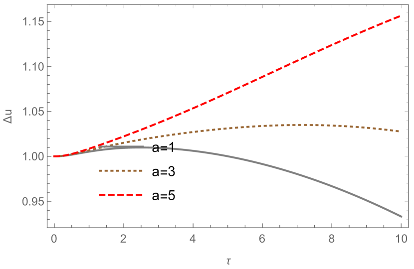
Figure 9: Variation of $\Delta u$ due to GW pulse has been presented with respect to $\tau$, for different choices of $a$ for Bardeen-Type black bounce.

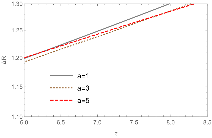
Figure 10: Variation of $\Delta R$ due to GW pulse with respect to $\tau$, for different choices of $a$ for Bardeen-Type black bounce.

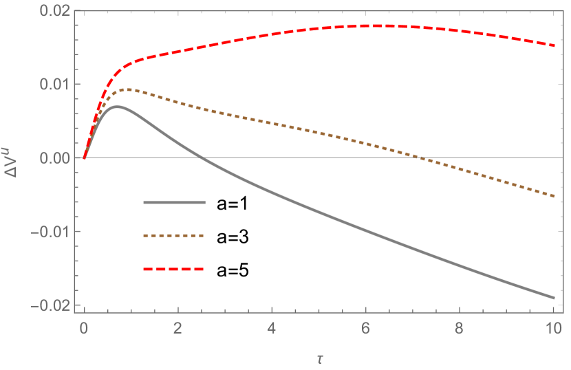
Figure 11: Variation of $\Delta V^{u}$ due to GW pulse with respect to $\tau$, for different choices of $a$ for Bardeen-Type black bounce.

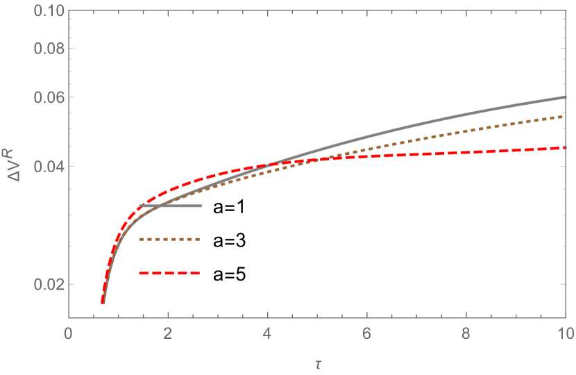
Figure 12: Variation of $\Delta V^{R}$ due to GW pulse with respect to $\tau$, for different choices of $a$ for Bardeen-Type black bounce.

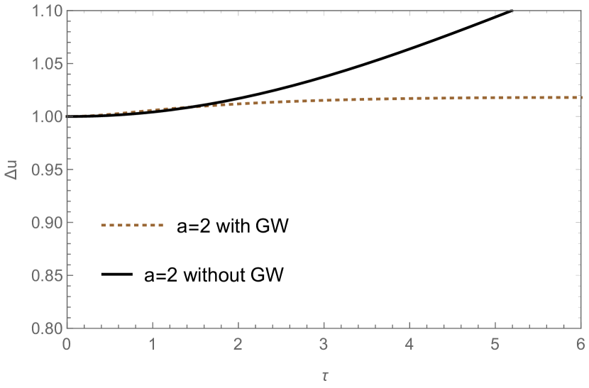
Figure 13: Variation of $\Delta u$ due to GW pulse and without GW pulse with respect to $\tau$ for Bardeen-Type black bounce.

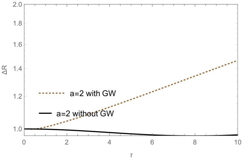
Figure 14: Variation of $\Delta R$ due to GW pulse and without GW pulse with respect to $\tau$ for Bardeen-Type black bounce.

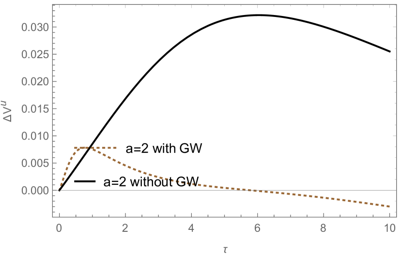
Figure 15: Variation of $\Delta V^{u}$ due to GW pulse and without GW pulse with respect to $\tau$ for Bardeen-Type black bounce.

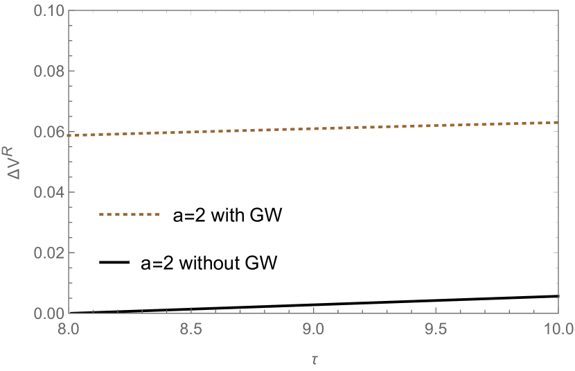
Figure 16: Variation of $\Delta V^{R}$ due to GW pulse and without GW pulse with respect to $\tau$ for Bardeen-Type black bounce.

The Bardeen-type black bounce solution described by the line element $(\ref{bouncemetric})$ and with

$$f(r)=1-\frac{2mr^{2}}{(r^{2}+a^{2})^{3/2}},~{}~{}~{}~{}~{}~{}~{}~{}~{}~{}and~{}~{}~{}~{}~{}~{}~{}~{}\sigma(r)=\sqrt{r^{2}+a^{2}}$$ (20)

In our previous discussion on the Simpson-Visser black bounce, we observed that the parameter $a$, representing the magnetic charge, plays a crucial role in preventing the emergence of a central singularity at $r=0$. Likewise, in the case of the Bardeen-Type solution, we encounter a parameter $a$ that serves as a regularization factor, effectively averting the formation of a singularity at $r=0$. The Kretschmann scalar associated with this solution can be expressed as follows.

$$R_{\mu\nu\rho\sigma}R^{\mu\nu\rho\sigma}=~{}~{}~{}~{}~{}~{}~{}~{}~{}~{}~{}~{}~{}~{}~{}~{}~{}~{}~{}~{}~{}~{}~{}~{}~{}~{}~{}~{}~{}~{}~{}~{}~{}~{}~{}~{}~{}~{}~{}~{}~{}~{}~{}~{}~{}~{}~{}~{}~{}~{}~{}~{}~{}~{}~{}~{}~{}~{}~{}~{}~{}~{}~{}~{}~{}~{}~{}~{}~{}~{}~{}~{}~{}~{}~{}~{}~{}~{}~{}~{}~{}~{}~{}~{}~{}~{}~{}~{}~{}~{}~{}~{}~{}~{}~{}~{}~{}~{}~{}~{}~{}~{}~{}~{}~{}~{}~{}~{}~{}~{}~{}~{}~{}~{}~{}~{}~{}~{}~{}~{}~{}~{}~{}~{}~{}~{}~{}~{}$$ (21)

$$\frac{m^{2}\left(16a^{8}-176a^{6}r^{2}+672a^{4}r^{4}-268a^{2}r^{6}+47r^{8}\right)-32ma^{2}r^{2}\sqrt{a^{2}+r^{2}}\left(2a^{4}+a^{2}r^{2}-r^{4}\right)+12a^{4}\left(a^{2}+r^{2}\right)^{3}}{\left(a^{2}+r^{2}\right)^{7}}$$

The finiteness of the Kretschmann scalar at $r=0$ is evident from the aforementioned expression, provided that $a\neq 0$. Hence, the parameter $a$ assumes a comparable significance to that in the Simpson-Visser scenario, thereby characterizing the solution as a black bounce.

In the Simpson-Visser solution, the discussion highlighted the need to consider geodesic memory effects in the Bardeen-Type background when a GW pulse is present. To account for this, the metric is expressed as a combination of the background metric, denoted as $g_{\mu\nu}$ and described by equation $(\ref{bouncemetric})$, and the perturbation caused by the GW pulse, represented as $h_{\mu\nu}$. To simplify the analysis, the transformation $R^{2}=r^{2}+a^{2}$ is applied to the metric $(\ref{bouncemetric})$. This transformation leads to the line element $(\ref{metricR})$ with the corresponding functions.

$$F(a,R)=1-\frac{2m}{R}+\frac{2ma^{2}}{R^{3}},$$ (22)

and

$$G(a,R)=\frac{R^{5}}{(R^{3}-2mR^{2}+2ma^{2})(R^{2}-a^{2})}$$ (23)

we define $Z(a,R)=\sqrt{G(a,R)F(a,R)}$ as follows

$$Z(a,R)=\sqrt{\frac{R^{2}}{R^{2}-a^{2}}}.$$ (24)

In this case, the metric $(\ref{metricRR})$ incorporates the variable $Z$. The definition of this metric relies on the transformation $u=t-r_{*}$, where $r_{*}$ represents the tortoise coordinate. The tortoise coordinate is determined by the transformation $(\ref{tor})$.

In this particular scenario, the perturbation of the metric $(\ref{metricRR})$ also results in a modified line element $(\ref{metricRRR})$. Additionally, within this model, we have defined $H(u)$ as the gravitational wave pulse, which can be expressed as $(\ref{Hu})$. On the equatorial plane $(\theta=\frac{\pi}{2})$, the geodesic equation for the $u$, $R$, and $\phi$ coordinates are given by equations $(\ref{14})$, $(\ref{15})$, and $(\ref{16})$, respectively. However, it is important to note that these equations incorporate the definitions $(\ref{F})$, $(\ref{G})$, and $(\ref{Z})$ for the functions $F$, $G$, and $Z$, respectively.

In the context of the Simpson-Visser solution, the displacement and velocity memory effects are also applicable to the Bardeen-Type black bounce. The Bardeen-Type solution, depicted as a black bounce, exhibits similar characteristics. Specifically, Figures (9) and (10) illustrate the values of $\Delta u$ and $\Delta R$ respectively. These figures demonstrate that as the magnetic charge $a$ increases, the difference between two adjacent geodesics for the component $u$ the displacement ($\Delta u$) also increases. Conversely, for the component $R$, the difference decreases as the magnetic charge $a$ increases, as shown in figure (10).

The changes observed in $R$ and $u$ can be interpreted as a memory effect related to displacement. On the other hand, the memory effect associated with velocity refers to the variation in the velocities of $u$ and $R$. These differences are determined by the variations of $\Delta u^{V}$ and $\Delta R^{V}$ with respect to $\tau$, as depicted in figures (11) and (12) respectively. It is worth noting that the changes in magnetic charge $a$ have a similar impact on the velocity memory effects as they do on the displacement memory effects.

Figures $(13)$ through $(16)$ offer a clear demonstration of the tangible GW pulse within the context of the Bardeen-Type black bounce. These figures showcase both the displacement and velocity memory effects. Specifically, figures $(13)$ and $(14)$ portray the changes in displacement memory effects when the GW pulse is either present or absent for a magnetic charge of $a=2$. Conversely, figures $(15)$ and $(16)$ illustrate the variations in $\Delta u^{V}$ and $\Delta R^{V}$ in the presence or absence of the GW pulse, once again for a magnetic charge of $a=2$. The geodesic deviation of two neighboring points decreases for the $u$ component of displacement and velocity memory effects when the GW pulse is present. However, this physical phenomenon is vice versa for the $R$ component.

IV A traversable wormhole solution and memory effects

Given that black bounce models already have wormhole solutions, our focus is now on exploring other wormhole solutions to examine their memory effects. In this particular section, we will investigate the gravitational memory effects of a special type of wormhole solution known as a traversable wormhole. To accomplish this, we will analyze the Einstein-Dirac-Maxwell (EDM) model. This model involves two gauged relativistic fermions, with opposite spins to maintain spherical symmetry. For a more comprehensive understanding of this model, readers can refer to the source 26 . In our analysis, we will work with units where $G=c=\hslash=1$, and the action of the corresponding EDM model can be expressed accordingly.

$$S=\frac{1}{4\pi}\int d^{4}x\sqrt{-g}[\frac{1}{4}R+L_{D}-\frac{1}{4}F^{2}],$$ (25)

The Dirac Lagrangian density for a charged spinor field coupled to an electromagnetic field is given by:

$$L_{D}=\sum_{\epsilon=1,2}[\frac{i}{2}\bar{\psi}{\epsilon}\gamma^{\nu}D{\nu}\psi_{\epsilon}-\frac{i}{2}D_{\nu}\bar{\psi}{\epsilon}\gamma^{\nu}\psi{\epsilon}-m\bar{\psi}{\epsilon}\psi{\epsilon}],$$ (26)

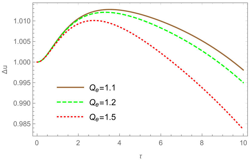
Figure 17: Variation of $\Delta u$ due to GW pulse has been presented with respect to $\tau$, for different choices of $Q_{e}$ of TWH ($m=1$ and $r_{0}=2$).

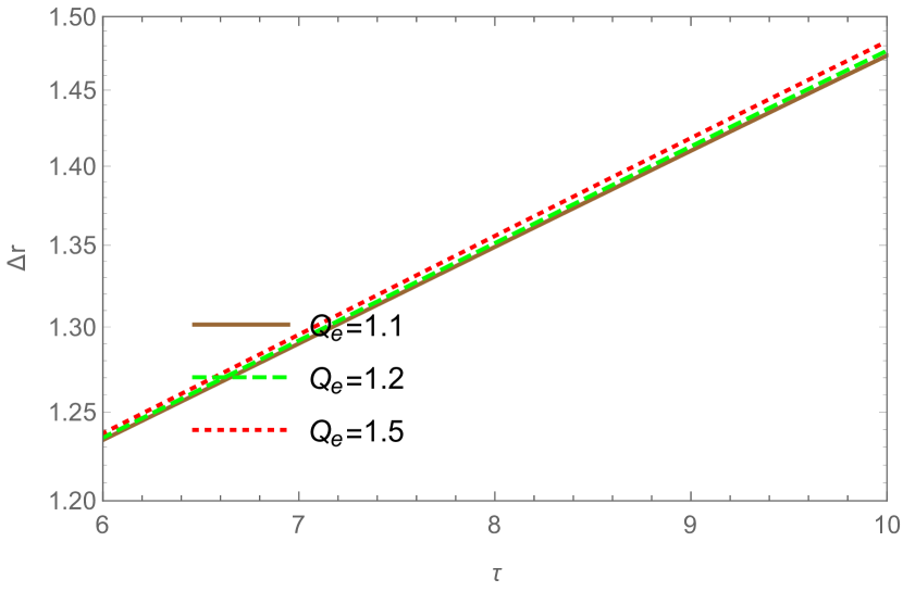
Figure 18: Variation of $\Delta r$ due to GW pulse with respect to $\tau$, for different choices of $Q_{e}$ of TWH.

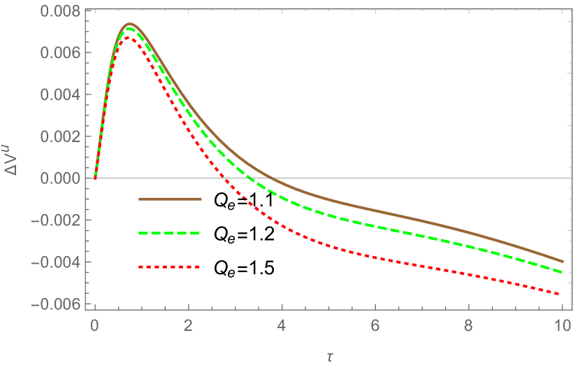
Figure 19: Variation of $\Delta V^{u}$ due to GW pulse with respect to $\tau$, for different choices of $Q_{e}$ of TWH.

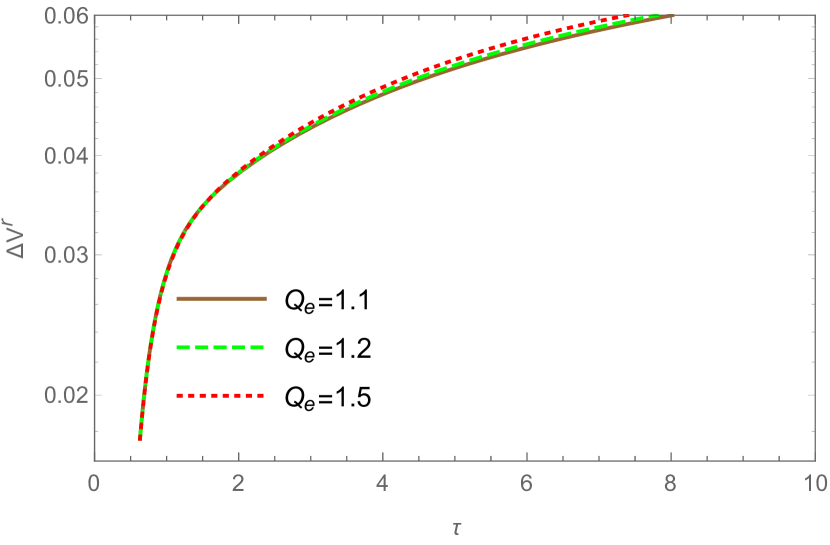
Figure 20: Variation of $\Delta V^{r}$ due to GW pulse with respect to $\tau$, for different choices of $Q_{e}$ of TWH.

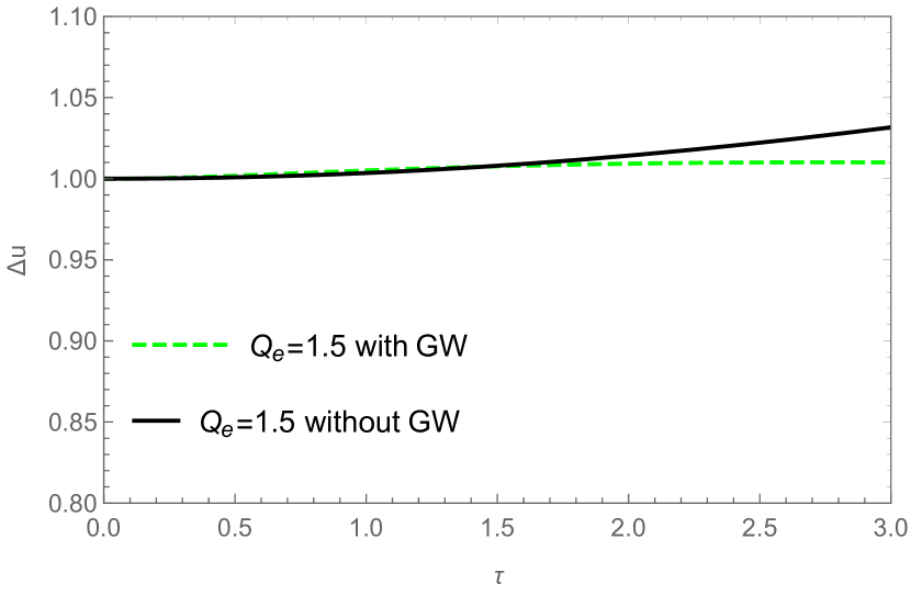
Figure 21: Variation of $\Delta u$ due to GW pulse and without GW pulse with respect to $\tau$ of TWH.

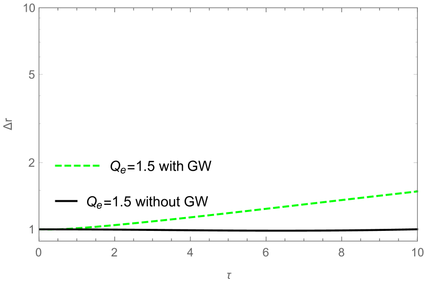
Figure 22: Variation of $\Delta r$ due to GW pulse and without GW pulse with respect to $\tau$ of TWH.

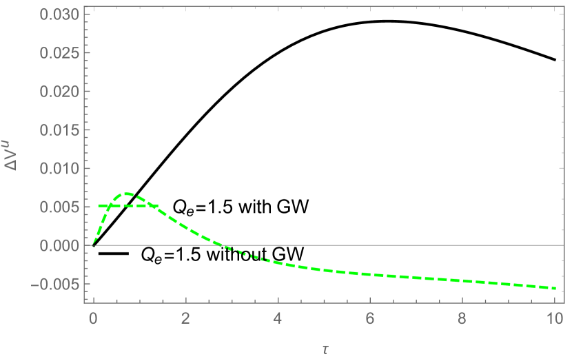
Figure 23: Variation of $\Delta V^{u}$ due to GW pulse and without GW pulse with respect to $\tau$ of TWH.

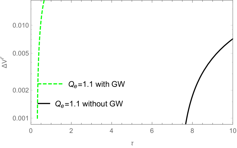
Figure 24: Variation of $\Delta V^{r}$ due to GW pulse and without GW pulse with respect to $\tau$ of TWH.

$R$ is the Ricci scalar of the metric $g_{\mu\nu}$, $F_{\mu\nu}=\partial_{\mu}A_{\nu}-\partial_{\nu}A_{\mu}$ is the field strength tensor, $L_{D}$ is the Dirac Lagrangian density, $\psi_{\epsilon}$ is the spinor field, $\gamma^{\nu}$ is the curved space $\gamma$ matrix, $D_{\mu}=\partial_{\mu}+\Gamma_{\mu}-ieA_{\mu}$ is the covariant derivative where $\Gamma_{\mu}$ and $e$ are the spinor connection matrices and the gauge coupling constant, respectively. $m$ is the mass of both spinors, and $i$ is the imaginary unit. Equation $(\ref{dirac})$ describes the interaction between the spinor field and the electromagnetic field in a curved spacetime.

By variation of action $(\ref{action0})$ with respect to the metric and fermion fields, the field equations are given by

$$R_{\mu\nu}-\frac{1}{2}Rg_{\mu\nu}=2T_{\mu\nu}~{}~{}~{}~{}~{}~{}~{}T_{\mu\nu}=T_{\mu\nu}^{D}+T_{\mu\nu}^{M}$$ (27)

$$(\gamma^{\nu}D_{\nu}-m)\psi_{\epsilon}=0~{}~{}~{}~{}~{}~{}and~{}~{}~{}~{}~{}\nabla_{\mu}F^{\mu\nu}=ej^{\nu}$$ (28)

In this context, the symbol $j^{\nu}$ represents the current, which is obtained by summing over the values of $\epsilon$ (which can be either 1 or 2) and multiplying the corresponding fermion fields $\bar{\psi}_{\epsilon}$, $\gamma^{\nu}$, and $\psi_{\epsilon}$

$$j^{\nu}=\sum_{\epsilon=1,2}\bar{\psi}_{\epsilon}\gamma^{\nu}\psi_{\epsilon}$$ (29)

On the other hand, the energy tensor $T_{\mu\nu}^{D}$ for the fermion field is calculated by summing over the values of $\epsilon$ (again, either 1 or 2), multiplying the imaginary part of $\bar{\psi}_{\epsilon}$, $\gamma_{(\mu}D_{\nu)}$, and $\psi_{\epsilon}$ by 2.

$$T_{\mu\nu}^{D}=\sum_{\epsilon=1,2}2Im(\bar{\psi}_{\epsilon}\gamma_{(\mu}D_{\nu)}\psi_{\epsilon})$$ (30)

Furthermore, the energy tensor for the Maxwell part is denoted as $T_{\mu\nu}^{M}$ and is determined by the expression $F_{\mu\alpha}F^{\alpha}_{\nu}-\frac{1}{4}F^{2}g_{\mu\nu}$, where $F_{\mu\alpha}$ represents the electromagnetic field tensor and $g_{\mu\nu}$ is the metric tensor.

Considering only static, spherically symmetric solutions of the field equations, we examine a comprehensive metric. We assume that the field $A$ is solely electric, given by $A=V(r)dt$, where $r$ and $t$ represent the radial and time coordinates, respectively. By imposing the conditions $e=0$, with vanishing frequency $\omega=0$, and assuming the massless spinor fields, the resulting EDM equations can be analytically solved. The solution encompasses the metric and the $U(1)$ potential 26 in the following manner.

$$ds^{2}=-(1-\frac{M}{r})^{2}dt^{2}+\frac{dr^{2}}{(1-\frac{r_{0}}{r})(1-\frac{Q_{e}^{2}}{r_{0}r})}+r^{2}d\Omega^{2}$$ (31)

$$V(r)=\frac{M}{Q_{e}}\sqrt{(1-\frac{r_{0}}{r})(1-\frac{Q_{e}^{2}}{r_{0}r})}$$ (32)

where $M$ is defined as

$$M=\frac{2Q_{e}^{2}r_{0}}{Q_{e}^{2}+r_{0}^{2}}.$$ (33)

This passage discusses a traversable wormhole (WH) solution, where the throat’s radius is denoted as $r_{0}$ and the electric charge $Q_{e}$ is less than $r_{0}$. with eleetrie charge. The WH solution is characterized by the Arnowitt-Deser-Misner (ADM) mass $M$, with the condition that $Q_{e}/M>1$. The WH geometry is sustained by the contribution of spinors to the total energy-momentum tensor, ensuring regularity throughout. As $Q_{e}$ approaches $r_{0}$, the WH solution transitions towards the extremal Reissner-Nordström (RN) black hole, while the contribution of $T_{\mu\nu}^{D}$ tends towards zero.

In this specific traversable Wormhole scenario, the conversation emphasized the importance of taking into account geodesic memory effects as displacement and velocity memory effects in the black bounce background (Simpson-Visser and Bardeen-Type) when a gravitational wave (GW) pulse is present. To address this, the metric is formulated as a combination of the background metric, denoted as $g_{\mu\nu}$ and defined by equation $(\ref{metricWH})$, and the perturbation induced by the GW pulse, represented as $h_{\mu\nu}$.

In order to achieve our objective, we proceed to the tortoise coordinate as in previous cases, which leads to the following line element:

$$ds^{2}=-f(r)du^{2}-2Z(r)dudr+r^{2}d\theta^{2}+r^{2}\sin^{2}\theta d\phi^{2}$$ (34)

Here, $Z(r)=\sqrt{g(r)f(r)}$ and the functions $f(r)$ and $g(r)$ are defined as:

$$f(r)=(1-\frac{M}{r})^{2}~{}~{}~{}~{}~{}and~{}~{}~{}~{}~{}~{}g(r)=\frac{1}{(1-\frac{r_{0}}{r})(1-\frac{Q_{e}^{2}}{r_{0}r})}$$ (35)

If we introduce the perturbation metric $h_{\mu\nu}$ to the background metric $(\ref{tortoiseWH})$, we obtain:

$$ds^{2}=-f(r)du^{2}-2Z(r)dudr+(r^{2}+rH(u))d\theta^{2}+(r^{2}-rH(u))\sin^{2}\theta d\phi^{2}.$$ (36)

In this case as well, we define $H(u)$ as the gravitational wave (GW) pulse, which takes the form $(\ref{Hu})$.

On the equatorial plane $(\theta=\frac{\pi}{2})$, the geodesic equations for the $u$ coordinate become:

$$\ddot{u}-\frac{f^{\prime}}{2Z}\dot{u}^{2}-\frac{H-2r}{2Z}\dot{\phi}^{2}=0$$ (37)

Here, $F$, $Z$, and $R$ are functions of $u$ and $\phi$. The geodesic equations for $r$ and $\phi$ are given by:

$$\ddot{r}+\frac{f}{2Z^{2}}f^{\prime}\dot{u}^{2}+\frac{f^{\prime}}{Z}\dot{r}\dot{u}+\frac{Z^{\prime}}{Z}\dot{r}^{2}+\frac{fH-2fr-rZH^{\prime}}{2Z^{2}}\dot{\phi}^{2}=0$$ (38)

$$\ddot{\phi}-\frac{H^{\prime}}{r-H}\dot{\phi}\dot{u}+\frac{2r-H}{r(r-H)}\dot{\phi}\dot{r}=0$$ (39)

where $H^{\prime}=\frac{dH}{du}$ and $f^{\prime}=\frac{df}{dr}$.

In our investigation of displacement and velocity memory effects, similar to previous cases, we focus on the deviation between two neighboring geodesics. In this particular study, we aim to explore the influence of electric charge, denoted as $Q_{e}$, on the gravitational memory effect. The reason behind considering the electric charge and its impact on gravitational memory lies in the unique nature of this charge. It is important to note that there is no presence of any ”real” charge in the given scenario. Instead, we have a purely geometric representation of electric charge, which is described in terms of the metric and topology of curved empty space. In other words, it is a charge without any physical charge. Therefore, the detection of traces of this type of charge in the gravitational memory serves as evidence supporting Wheeler’s concept of ”charge without charge” wheeler .

In this particular instance of traversable wormhole solution, similar to our previous solutions for black bounces, we observe the displacement memory effect denoted as $\Delta r$ and $\Delta u$, as well as the velocity memory effects represented by $\Delta V^{r}$ and $\Delta V^{u}$. These effects are obtained through numerical solutions of the equations $(\ref{WHu})$, $(\ref{WHr})$, and $(\ref{WHphi})$. Consequently, within this framework, we obtain the subsequent outcomes.

Figures (17) and (18) depict the variations in $\Delta u$ and $\Delta r$ correspondingly. These visual representations provide evidence that the disparity between two neighboring geodesics for the displacement component $u$ ($\Delta u$) diminishes with an increase in the electric charge $Q_{e}$. Conversely, for the component $r$, the difference decreases as the electric charge $Q_{e}$ decreases, as illustrated in figure (18).

The changes witnessed in $r$ and $u$ can be explained as a memory phenomenon linked to displacement. Conversely, the memory effect connected to velocity pertains to the variations in the velocities of $u$ and $r$. These disparities are influenced by the changes in $\Delta u^{V}$ and $\Delta R^{V}$ in relation to $\tau$, as illustrated in figures (19) and (20) respectively. It is important to highlight that the modifications in electric charge $Q_{e}$ have a comparable influence on the memory effects of velocity as they do on the memory effects of displacement.

Figures $(21)$ to $(24)$ provide a clear demonstration of the tangible gravitational wave (GW) pulse within the context of the traversable wormhole (WH). These figures showcase both the displacement and velocity memory effects. Specifically, figures $(21)$ and $(22)$ depict the changes in displacement memory effects when the GW pulse is either present or absent for an electric charge of $Q_{e}=1.5$. Conversely, figures $(23)$ and $(24)$ illustrate the variations in $\Delta u^{V}$ and $\Delta r^{V}$ in the presence or absence of the GW pulse, once again for an electric charge of $Q_{e}=1.5$. The geodesic deviation of two neighboring points decreases for the $u$ component of displacement and velocity memory effects when the GW pulse is present. However, this physical phenomenon is reversed for the $r$ component.

V Conclusion

The present study examines the gravitational memory effects, specifically the displacement and velocity memories, in the context of the black bounce and Einstein-Dirac-Maxwell traversable wormhole solutions. The investigation considers both in the presence and absence of a gravitational wave pulse. The findings reveal that in the case of the Simpson-Visser and Bardeen-Type black bounce solutions, the presence of a gravitational wave pulse leads to noticeable changes in the two neighboring geodesics. This phenomenon is also observed in the TWH solution, which incorporates fermion and Maxwell fields to enable traversability. In summary, the results demonstrate the impact of gravitational wave pulses on the behavior of geodesics in these solutions. We summarize the results as follows:

1- Simpson-Visser Solution: As the magnetic charge $a$ increases, the difference between two adjacent geodesics for the component $u$ $(\Delta u)$ decreases, while for the component $R$, the difference increases. These disparities can be interpreted as a displacement memory effect. The velocity memory effect refers to the changes in velocities of $u$ and $R$, determined by the variations of $\Delta u^{V}$ and $\Delta R^{V}$ with respect to $\tau$.

2-Bardeen-Type Black Bounce: Similar to the Simpson-Visser solution, the displacement and velocity memory effects are also applicable. As the magnetic charge a increases, the difference between two adjacent geodesics for the component $u$ $(\Delta u)$ increases, while for the component R, the difference decreases. The changes in $u$ and $R$ can be interpreted as a memory effect related to displacement. The velocity memory effect refers to the variation in the velocities of u and R, determined by the variations of $\Delta u^{V}$ and $\Delta R^{V}$ with respect to $\tau$.

3-Traversable Wormhole Solution: Similar to the previous solutions for black bounces, the displacement memory effect denoted as $\Delta r$ and $\Delta u$, as well as the velocity memory effects represented by $\Delta u^{V}$ and $\Delta r^{V}$ are observed. These effects are obtained through numerical solutions of certain equations.

In all cases, the presence or absence of a Gravitational Wave (GW) pulse also affects these memory effects. The figures mentioned in the text provide visual demonstrations of these phenomena.

References

- (1) R. D’Inverno, “Introducing Einstein’s Relativity”, Oxford University Press, New York (1998).
- (2) R. M. Wald, “General Relativity”, The University of Chicago Press, Chicago (1984).
- (3) A. Einstein, “Explanation of the Perihelion Motion of Mercury from the General Theory of Relativity”, Sitzungsber. Preuss. Akad. Wiss. Berlin (Math. Phys. ) 1915, 831-839 (1915).
- (4) G. V. Kraniotis and S. B. Whitehouse, “Exact calculation of the perihelion precession of mercury in general relativity, the cosmological constant and Jacobi’s inversion problem”, Class. Quant. Grav. 20, 4817-4835 (2003).
- (5) C. M. Will, “New General Relativistic Contribution to Mercury’s Perihelion Advance”, Phys. Rev. Lett. 120, no.19, 191101 (2018).
- (6) L. C. B. Crispino and D. Kennefick, “100 years of the first experimental test of General Relativity”, Nature Phys. 15, 416 (2019).
- (7) B. P. Abbott et al. [LIGO Scientific and Virgo], “Observation of Gravitational Waves from a Binary Black Hole Merger”, Phys. Rev. Lett. 116, no.6, 061102 (2016).
- (8) B. P. Abbott et al. [LIGO Scientific and Virgo], “GWTC-1: A Gravitational-Wave Transient Catalog of Compact Binary Mergers Observed by LIGO and Virgo during the First and Second Observing Runs”, Phys. Rev. X 9, no.3, 031040 (2019), [arXiv:1811.12907 [astro-ph.HE]].
- (9) R. Abbott et al. [LIGO Scientific and Virgo], “GWTC-2: Compact Binary Coalescences Observed by LIGO and Virgo During the First Half of the Third Observing Run”, Phys. Rev. X 11, 021053 (2021).
- (10) R. Abbott et al. [LIGO Scientific, VIRGO and KAGRA], “The population of merging compact binaries inferred using gravitational waves through GWTC-3”, [arXiv:2111.03634 [astro-ph.HE]].
- (11) P. Rastall, Phys. Rev. D 6, 3357 (1972).
- (12) S. Chandrasekhar, “The mathematical theory of black holes”, Published in Oxford University Press, New York (1992).
- (13) M. Visser, Lorentzian wormholes: From Einstein to Hawking, AIP press [now Springer], New York (1995).
- (14) A. Einstein and N. Rosen, “The Particle Problem in the General Theory of Relativity”, Phys. Rev. 48 (1935), 73-77.
- (15) H. G. Ellis, “Ether flow through a drain hole - a particle model in general relativity”, J. Math. Phys. 14 (1973), 104-118.
- (16) K. A. Bronnikov, “Scalar-tensor theory and scalar charge”, Acta Phys. Polon. B 4 (1973), 251-266.
- (17) M. S. Morris and K. S. Thorne, “Wormholes in space-time and their use for interstellar travel: A tool for teaching general relativity”, Am. J. Phys. 56 (1988), 395-412.
- (18) V. Cardoso, E. Franzin and P. Pani, “Is the gravitational-wave ringdown a probe of the event horizon?”, Phys. Rev. Lett. 116 (2016) no.17, 171101 [erratum: Phys. Rev. Lett. 117 (2016) no.8, 089902].
- (19) F. S. N. Lobo, “Phantom energy traversable wormholes”, Phys. Rev. D 71, 084011 (2005).
- (20) F. S. N. Lobo, “Exotic solutions in General Relativity: Traversable wormholes and warp drive spacetimes”, [arXiv:0710.4474 [gr-qc]].
- (21) M. Visser, S. Kar and N. Dadhich, “Traversable wormholes with arbitrarily small energy condition violations”, Phys. Rev. Lett. 90 (2003), 201102.
- (22) C. Barcelo and M. Visser, “Scalar fields, energy conditions, and traversable wormholes”, Class. Quant. Grav. 17 , 3843-3864 (2000).
- (23) K. A. Bronnikov, “Scalar fields as sources for wormholes and regular black holes”, Particles 1 no.1, 56-81, (2018).
- (24) K. A. Bronnikov, “Nonlinear electrodynamics, regular black holes, and wormholes”, Int. J. Mod. Phys. D 27 (2018) no.06, 1841005, [arXiv:1711.00087 [gr-qc]].
- (25) M. Alcubierre and F. S. N. Lobo, “Wormholes, Warp Drives, and Energy Conditions”, Fundam. Theor. Phys. 189 (2017), pp.-279 Springer, 2017, [arXiv:2103.05610 [gr-qc]].
- (26) J. L. Bl´azquez-Salcedo, C. Knoll and E. Radu, “Traversable wormholes in Einstein-Dirac-Maxwell theory”, Phys. Rev. Lett. 126 (2021) no.10, 101102, [arXiv:2010.07317 [gr-qc]].
- (27) S. Bolokhov, K. Bronnikov, S. Krasnikov, and M. Skvortsova, “A Note on “Traversable Wormholes in Einstein–Dirac–Maxwell Theory”, Grav. Cosmol. 27 (2021) no.4, 401-402, [arXiv:2104.10933 [gr-qc]].
- (28) R. A. Konoplya and A. Zhidenko, “Traversable Wormholes in General Relativity”, Phys. Rev. Lett. 128 (2022) no.9, 091104, [arXiv:2106.05034 [gr-qc]].
- (29) M. S. Churilova, R. A. Konoplya, Z. Stuchlik and A. Zhidenko, “Wormholes without exotic matter: quasinormal modes, echoes, and shadows”, JCAP 10 (2021), 010, [arXiv:2107.05977 [gr-qc]].
- (30) K. A. Bronnikov, R. A. Konoplya, and A. Zhidenko, “Instabilities of wormholes and regular black holes supported by a phantom scalar field”, Phys. Rev. D 86 (2012), 024028, [arXiv:1205.2224 [gr-qc]].
- (31) K. A. Bronnikov, L. N. Lipatova, I. D. Novikov and A. A. Shatskiy, “Example of a stable wormhole in general relativity”, Grav. Cosmol. 19 (2013), 269-274, [arXiv:1312.6929 [gr-qc]].
- (32) K. A. Bronnikov and S. Grinyok, “Instability of wormholes with a nonminimally coupled scalar field”, Grav. Cosmol. 7 (2001), 297-300, [arXiv:gr-qc/0201083 [gr-qc]].
- (33) F. S. N. Lobo, “Stability of phantom wormholes”, Phys. Rev. D 71 (2005), 124022, [arXiv:gr-qc/0506001 [gr-qc]].
- (34) M. Visser, “Traversable wormholes: Some simple examples”, Phys. Rev. D 39 (1989), 3182-3184, [arXiv:0809.0907 [gr-qc]].
- (35) J. P. S. Lemos, F. S. N. Lobo and S. Quinet de Oliveira, “Morris-Thorne wormholes with a cosmological constant”, Phys. Rev. D 68 (2003), 064004, [arXiv:gr-qc/0302049 [gr-qc]].
- (36) K. Jusufi and A. Ovg¨un, “Gravitational Lensing by Rotating Wormholes”, Ph ¨ ys. Rev. D 97 (2018) no.2, 024042, [arXiv:1708.06725 [gr-qc]].
- (37) J. G. Cramer, R. L. Forward, M. S. Morris, M. Visser, G. Benford and G. A. Landis, “Natural wormholes as gravitational lenses”, Phys. Rev. D 51 (1995), 3117-3120, [arXiv:astro-ph/9409051 [astro-ph]].
- (38) J. M. Bardeen, Non-singular general relativistic gravitational collapse, in Proceedings of the International Conference GR5, Tbilisi, U.S.S.R. (1968) .
- (39) E. Ayon-Beato and A. Garcia, “The Bardeen model as a nonlinear magnetic monopole”, Phys. Lett. B 493, 149-152 (2000), [arXiv:gr-qc/0009077 [gr-qc]].
- (40) K. A. Bronnikov, “Regular magnetic black holes and monopoles from nonlinear electrodynamics”, Phys. Rev. D 63, 044005 (2001), [arXiv:0006014 [gr-qc]].
- (41) M. E. Rodrigues, M. V. de S. Silva and H. A. Vieira, “Bardeen-Kiselev black hole with a cosmological constant”, Phys. Rev. D 105 (2022) no.8, 084043, [arXiv:2203.04965 [gr-qc]].
- (42) M. E. Rodrigues, M. V. de Sousa Silva and A. S. de Siqueira, “Regular multihorizon black holes in General Relativity”, Phys. Rev. D 102 (2020) no.8, 084038, [arXiv:2010.09490 [gr-qc]].
- (43) O. B. Zaslavskii, “Regular black holes and energy conditions”, Phys. Lett. B 688, 278-280 (2010), [arXiv:1004.2362 [gr-qc]].
- (44) M. E. Rodrigues, E. L. B. Junior, G. T. Marques and V. T. Zanchin, “Regular black holes in f(R) gravity coupled to nonlinear electrodynamics”, Phys. Rev. D 94 (2016) no.2, 024062, [arXiv:1511.00569 [gr-qc]].
- (45) M. E. Rodrigues, E. L. B. Junior and M. V. de S. Silva, “Using dominant and weak energy conditions for building new classes of regular black holes”, JCAP 02 (2018), 059, [arXiv:1705.05744 [physics.gen-ph]].
- (46) M. E. Rodrigues and M. V. d. Silva, “Bardeen Regular Black Hole With an Electric Source”, JCAP 06 (2018), 025, [arXiv:1802.05095 [gr-qc]].
- (47) M. E. Rodrigues and M. V. de S. Silva, “Regular multi-horizon black holes in f(G) gravity with nonlinear electrodynamics”, Phys. Rev. D 99 (2019) no.12, 124010, [arXiv:1906.06168 [gr-qc]].
- (48) M. V. d. Silva and M. E. Rodrigues, “Regular black holes in f(G) gravity”, Eur. Phys. J. C 78 (2018) no.8, 638, [arXiv:1808.05861 [gr-qc]].
- (49) E. L. B. Junior, M. E. Rodrigues and M. V. de Sousa Silva, “Regular black holes in Rainbow Gravity”, Nucl. Phys. B 961 (2020), 115244, [arXiv:2002.04410 [gr-qc]].
- (50) K. A. Bronnikov, “Comment on “Construction of regular black holes in general relativity””, Phys. Rev. D 96, no.12, 128501 (2017), [arXiv:1712.04342 [gr-qc]].
- (51) I. Dymnikova, “Regular electrically charged structures in nonlinear electrodynamics coupled to general relativity”, Classical Quantum Gravity 21, 4417 (2004), [arXiv:0407072 [gr-qc]].
- (52) J. C. S. Neves, A. Saa, “Regular rotating black holes and the weak energy condition”, Phys. Lett. B 734 (2014), 44-48, [arXiv:1402.2694 [gr-qc]].
- (53) B. Toshmatov, B. Ahmedov, A. Abdujabbarov, Z. Stuchlik, “Rotating Regular Black Hole Solution”, Phys. Rev. D 89 (2014) no. 10, 104017, [arXiv:1404.6443 [gr-qc]].
- (54) R. P. Bernar and L. C. B. Crispino, “Scalar radiation from a source rotating around a regular black hole”, Phys. Rev. D 100 (2019) no.2, 024012, [arXiv:1906.03778 [gr-qc]].
- (55) A. Simpson and M. Visser, “Black-bounce to traversable wormhole”, JCAP 02 (2019), 042, [arXiv:1812.07114 [gr-qc]].
- (56) F. S. N. Lobo, M. E. Rodrigues, M. V. de Sousa Silva, A. Simpson and M. Visser, “Novel black-bounce spacetimes: wormholes, regularity, energy conditions, and causal structure”, Phys. Rev. D 103, no.8, 084052 (2021), [arXiv:2009.12057 [gr-qc]].
- (57) E. L. B. Junior and M. E. Rodrigues, “Black-bounce in f(T) gravity”, Gen. Rel. Grav. 55 (2023) no.1, 8, [arXiv:2203.03629 [gr-qc]].
- (58) M. E. Rodrigues and M. V. d. S. Silva, “Black Bounces with multiple throats and anti-throats”, [arXiv:2204.11851 [gr-qc]].
- (59) H. Huang and J. Yang, “Charged Ellis Wormhole and Black Bounce”, Phys. Rev. D 100 (2019) no.12, 124063, [arXiv:1909.04603 [gr-qc]].
- (60) Y. Yang, D. Liu, Z. Xu and Z. W. Long, “Echoes from black bounces surrounded by the string cloud”, [arXiv:2210.12641[gr-qc]].
- (61) M. E. Rodrigues and M. V. d. S. Silva, “Embedding regular black holes and black bounces in a cloud of strings”, Phys.Rev. D 106, no.8, 084016 (2022), [arXiv:2210.05383 [gr-qc]].
- (62) H. C. D. Lima, Junior, C. L. Benone and L. C. B. Crispino, “Scalar scattering by black holes and wormholes”, Eur. Phys. J. C 82, no.7, 638 (2022), [arXiv:2211.09886 [gr-qc]].
- (63) S. Ghosh and A. Bhattacharyya, “Analytical study of gravitational lensing in Kerr-Newman black-bounce spacetime”, JCAP 11, 006 (2022), [arXiv:2206.09954 [gr-qc]].
- (64) J. Zhang and Y. Xie, “Gravitational lensing by a black-bounce-Reissner–Nordstr¨om spacetime”, Eur. Phys. J. C 82, no.5, 471 (2022).
- (65) Y. Yang, D. Liu, A. Ovg¨un, Z. W. Long and Z. Xu, “Quasinormal modes of Kerr-like ¨ black bounce spacetime”, [arXiv:2205.07530 [gr-qc]].
- (66) N. Tsukamoto, “Retrolensing by two photon spheres of a black-bounce spacetime”, Phys. Rev. D 105, no.8, 084036 (2022), [arXiv:2202.09641 [gr-qc]].
- (67) P. Bambhaniya, S. K, K. Jusufi and P. S. Joshi, “Thin accretion disk in the Simpson-Visser black-bounce and wormhole spacetimes”, Phys. Rev. D 105, no.2, 023021 (2022), [arXiv:2109.15054 [gr-qc]].
- (68) Z. Xu and M. Tang, “Rotating spacetime: black-bounces and quantum deformed black hole” Eur. Phys. J. C 81, no.10, 863 (2021), [arXiv:2109.13813 [gr-qc]].
- (69) Y. Yang, D. Liu, Z. Xu, Y. Xing, S. Wu and Z. W. Long, “Echoes of novel black-bounce spacetimes”, Phys. Rev. D 104, no.10, 104021 (2021), [arXiv:2107.06554 [gr-qc]].
- (70) M. Guerrero, G. J. Olmo, D. Rubiera-Garcia and D. S. C. G´ omez, “Shadows and optical appearance of black bounces illuminated by a thin accretion disk”, JCAP 08, 036 (2021), [arXiv:2105.15073 [gr-qc]].
- (71) N. Tsukamoto, “Gravitational lensing by two photon spheres in a black-bounce spacetime in strong deflection limits”, Phys. Rev. D 104, no.6, 064022 (2021), [arXiv:2105.14336 [gr-qc]].
- (72) E. Franzin, S. Liberati, J. Mazza, A. Simpson and M. Visser, “Charged black-bounce spacetimes”, JCAP 07, 036 (2021), [arXiv:2104.11376 [gr-qc]].
- (73) S. U. Islam, J. Kumar and S. G. Ghosh, “Strong gravitational lensing by rotating Simpson-Visser black holes”, JCAP 10, 013 (2021), [arXiv:2104.00696 [gr-qc]].
- (74) X. T. Cheng and Y. Xie, “Probing a black-bounce, traversable wormhole with weak deflection gravitational lensing”, Phys. Rev. D 103, no.6, 064040 (2021).
- (75) T. Y. Zhou and Y. Xie, “Precessing and periodic motions around a black-bounce/traversable wormhole”, Eur. Phys. J. C 80, no.11, 1070 (2020).
- (76) N. Tsukamoto, “Gravitational lensing in the Simpson-Visser black-bounce spacetime in a strong deflection limit”, Phys. Rev. D 103, no.2, 024033 (2021), [arXiv:2011.03932 [gr-qc]].
- (77) J. R. Nascimento, A. Y. Petrov, P. J. Porfirio and A. R. Soares, “Gravitational lensing in black-bounce spacetimes”, Phys. Rev. D 102, no.4, 044021 (2020), [arXiv:2005.13096 [gr-qc]].
- (78) F. S. N. Lobo, A. Simpson and M. Visser, “Dynamic thin-shell black-bounce traversable wormholes”, Phys. Rev. D 101, no.12, 124035 (2020), [arXiv:2003.09419 [gr-qc]].
- (79) Manuel E. Rodrigues and Marcos V. de S. Silva, Source of black bounces in general relativity, Phys. Rev. D 107, 044064 (2023).
- (80) P . M. Zhang, C. Duval, G. W. Gibbons, and P. A. Horvathy, Phys. Rev. D 96, 064013 (2017).
- (81) P. M. Zhang, C. Duval, G. W. Gibbons, and P. A. Horvathy, Phys. Lett. B 772, 743 (2017).
- (82) E. E. Flanagan, A. M. Grant, A. I. Harte, and D. A. Nichols, Phys. Rev. D 99, 084044 (2019).
- (83) I. Chakraborty and S. Kar, Phys. Rev. D 101, 064022 (2020).
- (84) I. Chakraborty and S. Kar, Phys. Lett. B 808, 135611 (2020).
- (85) S. Siddhant, I. Chakraborty, and S. Kar, Eur. Phys. J. C 81, 350 (2021).
- (86) I. Chakraborty, Phys. Rev. D 105, 024063 (2022).
- (87) P. Kanti, B. Kleihaus, and J. Kunz, Phys. Rev. Lett. 107, 271101 (2011).
- (88) D. J. Gross and J. H. Sloan, Nucl. Phys. B291, 41 (1987).
- (89) R. R. Metsaev and A. A. Tseytlin, Nucl. Phys. B293, 385 (1987).
- (90) Jose Luis Blázquez-Salcedo, Christian Knolland Eugen Radu, Traversable wormholes in Einstein-Dirac-Maxwell theory,PHYSICAL REVIEW LETTERS 126, 101102 (2021).
- (91) Bondi H 1960 Gravitational Waves in General Relativity Nature 186:535
- (92) Bondi H, van der Burg M G J and Metzner A W K 1962 Gravitational Waves in General Relativity, VII. Waves from Axi-Symmetric Isolated Systems Proceedings of the Royal Society of London Series A 269:21
- (93) Sachs R K 1962 Gravitational Waves in General Relativity. VIII. Waves in Asymptotically Flat Space-Time Proceedings of the Royal Society of London Series A, 270:103
- (94) Zel’dovich Y B and Polnarev A G 1974 Radiation of gravitational waves by a cluster of superdense stars Sov. Astron. 18 17
- (95) Braginsky V and Grishchuk L 1985 Kinematic Resonance and Memory Effect in Free Mass Gravitational Antennas Sov. Phys. JETP 62 427
- (96) Christodoulou D 1991 Nonlinear nature of gravitation and gravitational-wave experiments Phys. Rev. Lett. 67 1486
- (97) Thorne K S 1992 Gravitational-wave bursts with memory: The Christodoulou effect Phys. Rev. D 45 520
- (98) Strominger A and Zhiboedov A 2016 Gravitational Memory, BMS Supertranslations and Soft Theorems JHEP 01 086 [1411.5745]
- (99) Strominger A 2014 On BMS invariance of gravitational scattering JHEP 07 152 [1312.2229]
- (100) Pasterski S, Strominger A and Zhiboedov A 2016 New Gravitational Memories JHEP 12 053 [1502.06120]
- (101) Strominger A 2018 Lectures on the Infrared Structure of Gravity and Gauge Theory (Princeton University Press, [1703.05448])
- (102) Virgo and LIGO Scientific collaboration 2016 Observation of Gravitational Waves from a Binary Black Hole Merger Phys. Rev. Lett. 116 061102 [1602.03837]
- (103) Virgo and LIGO Scientific collaboration 2016 GW151226: Observation of Gravitational Waves from a 22-Solar-Mass Binary Black Hole Coalescence Phys. Rev. Lett. 116 241103 [1606.04855]
- (104) Virgo and LIGO Scientific collaboration 2017 GW170104: Observation of a 50-Solar-Mass Binary Black Hole Coalescence at Redshift 0.2 Phys. Rev. Lett. 118 221101 [1706.01812].
- (105) Virgo and LIGO Scientific collaboration 2017 GW170814: A Three-Detector Observation of Gravitational Waves from a Binary Black Hole Coalescence Phys. Rev. Lett. 119 141101 [1709.09660]
- (106) Virgo and LIGO Scientific collaboration 2017 GW170817: Observation of Gravitational Waves from a Binary Neutron Star Inspiral Phys. Rev. Lett. 119 161101 [1710.05832]
- (107) Virgo and LIGO Scientific Collaborations collaboration 2017 GW170608: Observation of a 19-solar-mass Binary Black Hole Coalescence Astrophys. J. 851 L35 [1711.05578].
- (108) Virgo and LIGO Scientific Collaborations collaboration 2019 GWTC-1: A Gravitational-Wave Transient Catalog of Compact Binary Mergers Observed by LIGO and Virgo during the First and Second Observing Runs Phys. Rev. X 9 031040 [1811.12907]
- (109) Virgo and LIGO Scientific Collaborations collaboration 2020 GW190425: Observation of a Compact Binary Coalescence with Total Mass 3:4M , Astrophys. J. Lett. 892 L3 [2001.01761]
- (110) J. A. Wheeler, Geometrodynamics (Academic, New York, 1962)