Reinforcement Learning from Human Feedback with Active Queries

Abstract

Aligning large language models (LLM) with human preference plays a key role in building modern generative models and can be achieved by reinforcement learning from human feedback (RLHF). Despite their superior performance, current RLHF approaches often require a large amount of human-labelled preference data, which is expensive to collect. In this paper, inspired by the success of active learning, we address this problem by proposing query-efficient RLHF methods. We first formalize the alignment problem as a contextual dueling bandit problem and design an active-query-based proximal policy optimization (APPO) algorithm with an $\widetilde{O}(d^{2}/\Delta)$ regret bound and an $\widetilde{O}(d^{2}/\Delta^{2})$ query complexity, where $d$ is the dimension of feature space and $\Delta$ is the sub-optimality gap over all the contexts. We then propose ADPO, a practical version of our algorithm based on direct preference optimization (DPO) and apply it to fine-tuning LLMs. Our experiments show that ADPO, while only making about half of queries for human preference, matches the performance of the state-of-the-art DPO method.

1 Introduction

Recent breakthroughs in large language models (LLM) significantly enhance performance across a diverse range of tasks, including commonsense reasoning, world knowledge, reading comprehension, math, code, and popular aggregated results (Jiang et al., 2023; Touvron et al., 2023; Chiang et al., 2023; Tunstall et al., 2023). In addition to their amazing capabilities in traditional natural language tasks (Gao et al., 2023a; Yuan et al., 2023; Han et al., 2023; Wei et al., 2023), they also demonstrate great potential in responding to human queries (Ouyang et al., 2022). One key step towards building these models is aligning them with human preference, where reinforcement learning from human feedback (RLHF) (Casper et al., 2023; Ouyang et al., 2022; Ziegler et al., 2019; Christiano et al., 2017; Rafailov et al., 2023) is widely employed. Typically, the process of RLHF is described as follows: At each time, the human user prompts the LLM with an instruction. Subsequently, the model generates several candidate responses and queries the users for their preferences. A reward model is then trained on this preference data to mimic human evaluation. The reward model can be parameterized by the language model itself (Rafailov et al., 2023) or by other neural networks (Gao et al., 2023b; Munos et al., 2023). The language models are then updated using reinforcement learning (RL) algorithms such as Proximal Policy Optimization (PPO) (Schulman et al., 2017) to optimize responses that maximize the reward.

Despite the notable success of RLHF in aligning language models with human preferences, its practical implementation often necessitates significant amounts of human-labeled preference data. For instance, the fine-tuning process of zephyr-7b-beta through RLHF relies on the utilization of a sizable 62k UltraCat-binarized dataset (Ding et al., 2023). The collection of such a substantial volume of human preference data is both costly and inefficient. Therefore, there exists a pressing need to develop query-efficient RLHF methods for effectively aligning large language models with human preferences.

Following recent theoretical advancements in RLHF (Xiong et al., 2023; Zhu et al., 2023; Sekhari et al., 2023), we formulate the RLHF problem as a contextual dueling bandit problem (Yue et al., 2012; Wu and Liu, 2016; Saha, 2021; Saha and Krishnamurthy, 2022; Saha and Gaillard, 2022; Wu et al., 2023; Di et al., 2023). In this setting, the learner proposes a pair of actions and receives noisy feedback regarding the preference between the dueling pair for each round. While numerous studies address regret minimization in dueling bandits, only Sekhari et al. (2023) have considered query complexity. However, the regret incurred by their algorithm exhibits a linear dependency on the size of the action set $\mathcal{A}$, limiting the practical applicability of their method.

In this paper, we adopt the principles of active learning (Zhang and Oles, 2000; Hoi et al., 2006) to design a query-efficient algorithm, Active Proximal Policy Optimization (APPO) for linear contextual dueling bandits. In each round, APPO employs the maximum likelihood estimator (Di et al., 2023) to estimate the underlying parameter and constructs an optimistic estimator for the reward gap between different arms. Subsequently, APPO selects the best arms and estimates the uncertainty associated with the potential feedback. To reduce the query complexity, APPO selectively queries the dueling preference and updates the estimation only when the uncertainty of the observation exceeds a threshold.

We further extend APPO to direct preference optimization (DPO) (Rafailov et al., 2023) and introduce a novel query-efficient method, Active Direct Policy Optimization (ADPO). Following the methodology of APPO, ADPO selectively queries human preference only for data where the model exhibits high uncertainty about the observation. For data where the model is less uncertain about, we employ the pseudo label predicted by the model to fine-tune the model itself.

• We propose an active-learning based algorithm APPO for linear contextual dueling bandits with a global sub-optimal gap. Theoretical analysis shows that our algorithm enjoys a constant regret $\widetilde{O}(d^{2}/\Delta)$. Meanwhile, our proposed algorithm only requires $\widetilde{O}(d^{2}/\Delta^{2})$ queries in total $T$ rounds, where $d$ is the dimension of the feature mapping, and $\Delta$ is the sub-optimal gap. Compared with previous regret bound $\widetilde{O}(\min\{\sqrt{AT\beta},A^{2}\beta^{2}d/\Delta\})$ achieved by Sekhari et al. (2023), our regret bound is independent on the size of action space $A$, which is more favorable in practice.

• We propose an active learning-based DPO method, ADPO. We apply our method to train zephyr-7b-beta on UltraCat-binarized dataset (Ding et al., 2023). Our experiment shows while ADPO only make about half numbers of queries, the model trained by ADPO outperforms DPO on Open-LLM-Benchmark (Beeching et al., 2023) by a margin of 0.35%.

Notation.

We employ $[n]$ to denote the set $\{1,\dots,n\}$. In this work, we use lowercase letters to represent scalars, and denote vectors and matrices by lower and uppercase boldface letters respectively. Given a vector $\mathbf{x}\in\mathbb{R}^{d}$, we denote the vector’s $L_{2}$-norm by $\|\mathbf{x}\|_{2}$. We further define $\|\mathbf{x}\|_{\bm{\Sigma}}=\sqrt{\mathbf{x}^{\top}\bm{\Sigma}\mathbf{x}}$ given a positive semidefinite matrix $\bm{\Sigma}\in\mathbb{R}^{d\times d}$. We use standard asymptotic notations $O(\cdot),\Omega(\cdot),\Theta(\cdot)$, and further use $\widetilde{O}(\cdot)$ to hide polylogarithmic factors other than the number of rounds $T$. We use $\operatorname{\mathds{1}}\{\cdot\}$ denote the indicator function,

2 Related Work

2.1 Reinforcement Learning from Human Feedback

Learning from human preference data dates back to Wirth et al. (2017); Christiano et al. (2017) and is recently popularized by generative language models (Achiam et al., 2023; Touvron et al., 2023). This procedure usually takes place after supervised finetuning (SFT). The canonical procedure of aligning with human preference includes two steps: reward modeling and reward maximization (Ouyang et al., 2022; Bai et al., 2022; Munos et al., 2023). Another approach is direct preference optimization (DPO) (Rafailov et al., 2023), which treats the generative models directly as reward models and trains them on preference data. Compared with the first approach, DPO simplifies the alignment process while maintaining its effectiveness. However, both paradigms require a large amount of human preference data. In this work, we follow the DPO approach and propose a query-efficient DPO.

The empirical success of RLHF also prompts a series of theoretical works, with a predominant focus on the reward maximization stage, modeling this process as learning a dueling bandit (Zhu et al., 2023; Xiong et al., 2023; Sekhari et al., 2023). Among these works, Sekhari et al. (2023) stands out for considering query complexity in the process. However, their regret bound is $\widetilde{O}(\min\{\sqrt{AT\beta},A^{2}\beta^{2}d/\Delta\})$, depending on the size of the action set $A$, thereby limiting the practical applicability of their algorithm.

2.2 Dueling Bandits

Dueling bandits represent a variant of the multi-armed bandit, incorporating preference feedback between two selected arms (Yue et al., 2012). Existing results in this domain generally fall into two categories, shaped by their assumptions about preference probability. The first category of work (Yue et al., 2012; Falahatgar et al., 2017, 2018; Ren et al., 2019; Wu et al., 2022; Lou et al., 2022) assumes a transitivity property for preference probability and focuses on identifying the optimal action. Our work also belongs to this category. The second category of work (Jamieson et al., 2015; Heckel et al., 2018; Saha, 2021; Wu et al., 2023; Dudík et al., 2015; Ramamohan et al., 2016; Balsubramani et al., 2016) focuses on general preferences with various criteria for optimal actions, such as Borda winner and Copeland winner.

Expanding beyond the standard dueling bandit problem, Dudík et al. (2015) was the first to incorporate contextual information into the dueling bandit framework. Subsequently, Saha (2021) studied the $K$-arm contextual dueling bandit problem and proposed an algorithm with a near-optimal regret guarantee. In order to address the challenge of a potentially large action space, Bengs et al. (2022) also considered linear function approximation and extended these results to the contextual linear dueling bandit problem and obtained a regret guarantee of $\widetilde{O}(d\sqrt{T})$. Recently, Di et al. (2023) introduced a layered algorithm, improving the results to a variance-aware guarantee of $\widetilde{O}(d\sqrt{\sum\sigma_{t}^{2}})$, where $\sigma_{t}^{2}$ denotes the variance of the observed preference in round $t$.

2.3 Active Learning

To mitigate the curse of label complexity, active learning serves as a valuable approach in supervised learning . The first line of work is pool-based active learning (Zhang and Oles, 2000; Hoi et al., 2006; Gu et al., 2012, 2014; Citovsky et al., 2021). In pool-based active learning, instead of acquiring labels for the entire dataset, the learner strategically selects a batch of the most informative data at each step and exclusively queries labels for this selected data batch. The learner then employs this labeled data batch to update the model. Subsequently, guided by the enhanced model, the learner queries another mini-batch of labels and continues the training process. These steps are iteratively repeated until the model achieves the desired performance level. The strategic selection of informative data in active learning significantly reduces the label complexity for supervised learning. The label complexity of pool-based active learning has been extensively studied by Dasgupta (2005); Dasgupta et al. (2005); Balcan et al. (2006, 2007); Hanneke and Yang (2015); Gentile et al. (2022). On the other hand, selective sampling (a.k.a., online active learning) (Cesa-Bianchi et al., 2005, 2006, 2009; Hanneke and Yang, 2021) is a learning framework that integrates online learning and active learning. In this framework, the algorithm sequentially observes different examples and determines whether to collect the label for the observed example. minimizing the total regret with more collected data

Another line of research (Schulze and Evans, 2018; Krueger et al., 2020; Tucker et al., 2023) focused on active reinforcement learning and directly integrates the query cost into the received reward. Krueger et al. (2020) laid the groundwork for active reinforcement learning by introducing a cost $c$ associated with each reward observation and evaluated various heuristic algorithms for active reinforcement learning. Recently, Tucker et al. (2023) studied the multi-arm bandit problem with costly reward observation. Their work not only suggests empirical advantages but also proves an $O(T^{2/3})$ regret guarantee.

3 Preliminaries

In this work, we formulate the RLHF problem as a contextual dueling bandit problem (Saha, 2021; Di et al., 2023). We assume a context set $\mathcal{X}$, and at the beginning of each round, a contextual variable $x_{t}$ is i.i.d generated from the context set $\mathcal{X}$ following the distribution $\mathcal{D}$. Based on the context $x_{t}$, the learner then chooses two actions $y_{t}^{1},y_{t}^{2}$ from the action space $\mathcal{A}$ and determines whether to query the environment for preferences between these actions. If affirmative, the environment generates the preference feedback $o_{t}$ with the following probability $\mathbb{P}(o_{t}=1|x_{t},y_{t}^{1},y_{t}^{2})=\mu\big{(}r(x_{t},y_{t}^{1})-r(x_{t},y_{t}^{2})\big{)}$, where $\mu(\cdot):\mathbb{R}\rightarrow[0,1]$ is the link function and $r(\cdot,\cdot)$ is the reward model.

We consider the linear reward model, i.e., $r(x,y)=\langle\bm{\theta}^{*},\bm{\phi}(x,y)\rangle$, where $\bm{\theta}^{*}\in\mathbb{R}^{d}$ and $\bm{\phi}:\mathcal{X}\times\mathcal{A}\rightarrow\mathbb{R}^{d}$ is a known feature mapping. For the sake of simplicity, we use $\bm{\phi}_{t}^{1},\bm{\phi}_{t}^{2}$ to denote $\bm{\phi}(x_{t},y_{t}^{1}),\bm{\phi}(x_{t},y_{t}^{2})$. Additionally, we assume the norm of the feature mapping $\bm{\phi}$ and the underlying vector $\bm{\theta}^{*}$ are bounded.

Assumption 3.1.

The linear contextual dueling bandit satisfies the following conditions:

• For any contextual $x\in\mathcal{X}$ and action $y\in\mathcal{A}$, we have $\|\bm{\phi}(x,y)\|_{2}\leq L/2$.

• For the unknown environment parameter $\bm{\theta}^{*}$, it satisfies $\|\bm{\theta}^{*}\|_{2}\leq B$.

For the link function $\mu$, we make the following assumption, which is commonly employed in the study of generalized linear contextual bandits (Filippi et al., 2010; Di et al., 2023).

Assumption 3.2.

The link function $\mu$ is differentiable and the corresponding first derivative satisfies

$$\kappa_{\mu}\leq\dot{\mu}(\cdot),$$

where $\kappa_{\mu}>0$ is a known constant.

The learning objective is to minimize the cumulative regret defined as:

$$\text{Regret}(T)=\sum_{t=1}^{T}r^{*}(x_{t})-r(x_{t},y_{t}^{1}),$$

where $r^{*}(x_{t})=r^{*}(x_{t},y_{t}^{*})=\max_{y\in\mathcal{A}}r^{*}(x_{t},y)$ stands for the largest possible reward in context $x_{t}$. In comparison with prior studies (Saha, 2021; Di et al., 2023), our regret measure only focuses on the gap between action $y_{t}^{1}$ and the optimal action $y_{t}^{*}$. In the context of RLHF, the model generates multiple candidate responses, and users will choose the most preferable response from the available options. Under this situation, sub-optimality is only associated with the selected response and therefore we focus on the regret from action $y_{t}^{1}$.

To quantify the cost of collecting human-labeled data, we introduce the concept of query complexity $\text{Query}(T)$ for an algorithm, which is the total number of data pairs that require human feedback for preference across the first $T$ rounds. It is worth noting that while some prior work (Tucker et al., 2023) incorporates direct costs $c$ in the reward for required human feedback, in our work, we distinguish between regret and query complexity as two separate performance metrics for an algorithm.

In addition, we consider the minimal sub-optimality gap (Simchowitz and Jamieson, 2019; Yang et al., 2020; He et al., 2021), which characterizes the difficulty of the bandit problem.

Definition 3.3 (Minimal sub-optimality gap).

For each context $x\in\mathcal{X}$ and action $y\in\mathcal{A}$, the sub-optimality gap $\Delta(x,y)$ is defined as

$$\Delta(x,y)=r^{*}(x)-r(x,y),$$

and the minimal sub-optimality gap is defined as

$$\Delta=\min_{x\in\mathcal{X},y\in\mathcal{A}}\big{\{}\Delta(x,y):\Delta(x,y)\neq 0\big{\}}.$$

In general, a larger sub-optimality gap $\Delta$ between action $y$ and the optimal action $y^{*}$ implies that it is easier to distinguish between these actions and results in a lower cumulative regret. Conversely, a task with a lower gap $\Delta$ indicates that it is more challenging to make such a distinction, leading to a larger regret. In this paper, we assume the minimal sub-optimality gap is strictly positive.

Assumption 3.4.

The minimal sub-optimality gap is strictly positive, i.e., $\Delta>0$.

Algorithm 1 Acitve Proximal Policy Optimization (APPO)

0:  Regularization parameter $\lambda>0$, and $B$, an upper bound on the $\ell_{2}$-norm of $\bm{\theta}^{*}$, confidence radius $\beta$, uncertainty threshold $\Gamma$, learning rate $\eta$

1:  Set initial policy $\pi_{1}(\cdot|\cdot)$ as uniform distribution over the action set $\mathcal{A}$, $\bm{\Sigma}_{0}\leftarrow\lambda\mathbf{I}$, $\mathcal{C}_{0}=\emptyset$

2:  for $t=1,\ldots,T$ do

3:     Compute the MLE $\widehat{\bm{\theta}}_{t}$ as in (4.1) and observe $\mathcal{A}$, select $y_{t}^{2}\sim\text{Uniform}(\mathcal{A})$

4:     Let $\widehat{D}_{t}(x_{t},y)=\min\bigl{\{}\langle\widehat{\bm{\theta}}_{t},\bm{\phi}(x_{t},y)-\bm{\phi}^{2}_{t}\rangle+\beta\|\bm{\phi}(x_{t},y)-\bm{\phi}^{2}_{t}\|_{\bm{\Sigma}_{t-1}^{-1}},2\bigr{\}}$

5:     Let $y^{1}_{t}=\mathop{\mathrm{argmax}}_{y}\widehat{D}_{t}(x_{t},y)$

6:     if $\|\bm{\phi}^{1}_{t}-\bm{\phi}^{2}_{t}\|_{\bm{\Sigma}_{t-1}}\leq\Gamma$ then

7:        play the duel $(y^{1}_{t},y^{2}_{t})$ and keep $\bm{\Sigma}_{t}=\bm{\Sigma}_{t-1}$

8:        $\pi_{t+1}(y|x)=\pi_{t}(y|x)$, $\mathcal{C}_{t}=\mathcal{C}_{t-1}$

9:     else

10:        Sample $y^{1}_{t}\sim\pi_{t}(\cdot|s_{t})$ and play the duel $(y^{1}_{t},y^{2}_{t})$, $\mathcal{C}_{t}=\mathcal{C}_{t-1}\cup\{t\}$

11:        Query for the preference and observe $o_{t}$

12:        Update $\bm{\Sigma}_{t}=\bm{\Sigma}_{t-1}+(\bm{\phi}^{1}_{t}-\bm{\phi}^{2}_{t})(\bm{\phi}^{1}_{t}-\bm{\phi}^{2}_{t})^{\top}$

13:        Update $\pi_{t+1}(y|x)\propto\pi_{t}(y|x)\exp\big{(}\eta\widehat{D}_{t}(x,y)\big{)}$

14:     end if

15:  end for

4 Algorithm

In this section, we introduce our proposed query-efficient method for aligning LLMs. The main algorithm is illustrated in Algorithm 1. At a high level, the algorithm leverages the uncertainty-aware query criterion (Zhang et al., 2023) to issue queries and employs Optimistic Proximal Policy Optimization (OPPO) (Cai et al., 2020; He et al., 2022b) for policy updates. In the sequel, we introduce the key parts of the proposed algorithm.

4.1 Regularized MLE

For each round $t\in[T]$, we construct the regularized maximum likelihood estimator (MLE) (Line 3) of parameter $\bm{\theta}^{*}$ by solving the following equation:

$$\lambda\bm{\theta}+\sum_{\tau\in\mathcal{C}_{t-1}}\big{(}o_{\tau}-\mu(\langle\bm{\theta},\bm{\phi}^{1}_{\tau}-\bm{\phi}^{2}_{\tau}\rangle)\big{)}(\bm{\phi}^{1}_{\tau}-\bm{\phi}^{2}_{\tau})=\mathbb{0},$$ (4.1)

where $\mathcal{C}_{t}$ represents the index set of rounds up to round $t$ with human-labelled preferences, initially set as an empty set. Compared with previous work on linear dueling bandits (Di et al., 2023), only part of the data requires human-labelled preference and we construct the MLE only with rounds $t\in\mathcal{C}_{T}$. In addition, the estimation error between $\widehat{\bm{\theta}}_{t}$ and $\bm{\theta}^{*}$ satisfied

$$\|\widehat{\bm{\theta}}_{t}-\bm{\theta}^{*}\|_{\Sigma_{t-1}}\leq\widetilde{O}\big{(}\sqrt{d\log|\mathcal{C}_{T}|}/\kappa_{\mu}\big{)}.$$

After constructing the estimator $\widehat{\bm{\theta}}_{t}$, the agent first selects a baseline action $y^{2}_{t}$ and compares each action $y\in\mathcal{A}$ with the baseline action $y_{t}^{2}$. For simplicity, we denote $D_{t}(x_{t},y)=\langle\bm{\theta}^{*},\bm{\phi}(x_{t},y)-\bm{\phi}^{2}_{t}\rangle$ as the reward gap between $y$ and action $y_{t}^{2}$. Then, we construct an optimistic estimator $\widehat{D}_{t}$ (Line 4) for the reward gap with linear function approximation and Upper Confidence Bound (UCB) bonus, i.e.,

$$\widehat{D}_{t}(x_{t},y)\approx\langle\widehat{\bm{\theta}}_{t},\bm{\phi}(x_{t},y)-\bm{\phi}^{2}_{t}\rangle+\beta\|\bm{\phi}(x_{t},y)-\bm{\phi}^{2}_{t}\|_{\bm{\Sigma}_{t-1}^{-1}}.$$

With the help of UCB bonus, we can show that our estimated reward gap $\widehat{D}_{t}$ is an upper bound of the true reward gap $D_{t}$.

4.2 Uncertainty-Aware Query Criterion

To mitigate the expensive costs from collecting human feedback, we introduce the uncertainty-based criterion (Line 6) (Zhang et al., 2023) to decide whether a pair of action requires $y_{t}^{1}$ and $y_{t}^{2}$ requires human-labelled preference. Similar criterion has also been used in corruption-robust linear contextual bandits (He et al., 2022c) and achieving nearly minimax optimal regret in learning linear (mixture) Markov decision processes (Zhou and Gu, 2022; He et al., 2022a; Zhao et al., 2023). Intuitively speaking, the UCB bonus $\beta\|\bm{\phi}_{t}^{1}-\bm{\phi}_{t}^{2}\|_{\bm{\Sigma}_{t-1}^{-1}}$ captures the uncertainty associated with the preference feedback $o_{t}$. For the action pair $(y_{t}^{1},y_{t}^{2})$ with low uncertainty, where the observation is nearly known and provides minimal information, we select the action $y_{t}^{1},y_{t}^{2}$ without querying human preference feedback. In this situation, the policy $\pi(\cdot|\cdot)$ remains unchanged as there is no observation in this round. By employing the uncertainty-based data selection rule, we will later prove that the query complexity is effectively controlled by:

$$\textbf{Query}(T)=|\mathcal{C}_{T}|\leq\widetilde{O}(d^{2}/\Delta^{2}).$$

4.3 Proximal Policy Optimization

In cases where the action pair $(y_{t}^{1},y_{t}^{2})$ exhibits high uncertainty and the uncertainty-aware query criterion is triggered, the agent resample the action $y_{t}^{1}$ from policy $\pi_{t}$ and queries human feedback for the duel $y_{t}^{1},y_{t}^{2}$. Upon observing the preference $o_{t}$, this round is then added to the index set $\mathcal{C}_{t}$. Subsequently, the policy $\pi_{t+1}$ is updated using the Proximal Policy Optimization (PPO) method (Line 13), i.e.,

$$\pi_{t+1}(y|x)\propto\pi_{t}(y|x)\exp\big{(}\eta\widehat{D}_{t}(x,y)\big{)}.$$

In an extreme case where the uncertainty threshold $\Gamma$ is chosen to be $0$, the uncertainty-aware query criterion will always be triggered. Under this situation, Algorithm 1 will query the human-labeled preference for each duel $(y_{t}^{1},y_{t}^{2})$, and it will degenerate to the dueling bandit version of OPPO (Cai et al., 2020). In this case, Algorithm 1 has $\widetilde{O}(d\sqrt{T})$ regret while having a linear query complexity in the number of rounds $T$.

5 Theoretical Analysis

In this section, we present our main theoretical results.

Theorem 5.1.

Under Assumption 3.4, if we set the parameters $\Gamma=\widetilde{O}(\Delta/\sqrt{{d}})$, $\lambda=B^{-2}$, $\eta=\widetilde{O}(\sqrt{\Gamma^{2}\log\mathcal{A}/d})$, and $\beta=\widetilde{O}(\sqrt{d}/\kappa_{\mu})$ in Algorithm 1, then with probability at least $1-\delta$, the regret for Algorithm 1 in the first $T$ rounds is upper bounded by

$$\text{Regret}(T)=\widetilde{O}(d^{2}/\Delta).$$

In addition, the query complexity of Algorithm 1 is upper bounded by

$$\textbf{Query}(T)=\widetilde{O}(d^{2}/\Delta^{2}).$$

Remark 5.2.

Theorem 5.1 suggests that our algorithm achieves a constant regret and query complexity that is independent of $T$. It is important to highlight that our algorithm requires a prior knowledge of the sub-optimal gap $\Delta$. Under the situation where $\Delta$ is unknown, the learner can set the parameter $\Delta$ via grid search process.

Remark 5.3.

In comparison with the regret $\widetilde{O}(A^{2}d/\Delta)$ obtained by the AURORA algorithm (Sekhari et al., 2023), our algorithm’s regret eliminates the dependency on the action space $A$. In comparison to the query complexity $\widetilde{O}(A^{3}d^{2}/\Delta^{2})$ in Sekhari et al. (2023), we achieve a query complexity improvement by a factor of $A^{3}$.

6 Practical Algorithm

Algorithm 2 Active Direct Preference Optimization (ADPO)

0:  Regularization parameter $\beta$, uncertainty threshold $\Gamma$, learning rate $\eta$, initial model parameter $\bm{\theta}_{0}$, batch size $B$

1:  Set $\bm{\theta}\leftarrow\bm{\theta}_{0}$

2:  for $t=1,\ldots,T$ do

3:     Receive batch of data $\mathcal{B}_{t}=\{x_{i},y_{i}^{1},y_{i}^{2}\}_{i=1}^{B}$

4:     for $i=1,\ldots,B$ do

5:        Compute or query the preference label $o_{i}$ based on (6.2)

6:     end for

7:     Update $\bm{\theta}\leftarrow\bm{\theta}-\eta\nabla_{\bm{\theta}}\mathcal{L}_{\mathcal{B}_{t}}(\pi_{\bm{\theta}},\pi_{\bm{\theta}_{0}})$

8:  end for

In this section, we introduce a practical version of our proposed algorithm, namely active direct preference optimization (ADPO) and summarize it in Algorithm 2. Inspired from Algorithm 1 and direct preference optimization (DPO) (Rafailov et al., 2023), ADPO is an active learning-based DPO. In this section, we consider the Bradley-Terry-Luce model (Bradley and Terry, 1952), where the link function has the form $\mu(x)=1/(1+e^{-x})$. At a high level, ADPO follows the basic idea of Algorithm 1 and sets an uncertainty threshold to select data for querying human preferences. However, adapting our algorithm to LLM fine-tuning requires several key modifications as outlined below.

Direct Preference Optimization.

We follow the framework of DPO (Rafailov et al., 2023) for LLM alignment. In DPO, the reward is directly parameterized by the language model in the following way:

$$r_{\bm{\theta}}(x,y)=\beta\big{(}\log\pi_{\bm{\theta}}(y|x)-\log\pi_{\text{ref}}(y|x)\big{)},$$

where $\beta$ is a regularization parameter, $y$ is a possible answer given the prompt $x$ and $\pi_{\text{ref}}$ is the reference model, which is usually the SFT checkpoint in practice. With the reward model parameterized above, we have the following DPO training objective:

$$\mathcal{L}_{\text{DPO}}(\pi_{\bm{\theta}},\pi_{\text{ref}})=-\mathbb{E}_{(x,y^{1},y^{2},o)\sim\mathcal{D}}\Big{[}\log\mu\Big{(}o\cdot\big{(}r_{\bm{\theta}}(x,y^{1})-r_{\bm{\theta}}(x,y^{2})\big{)}\Big{)}\Big{]},$$

where $\mathcal{D}$ is the data distribution, $y^{1}$ and $y^{2}$ are the two answers given the prompt $x$, and $o$ is the human preference such that $o=1$ indicates a preference for $y^{1}$, and $o=-1$ indicates a preference for $y^{2}$. This approach bypasses the reward-model training process in standard RLHF and, therefore, eliminates the reward estimation error introduced in it. We follow this approach and treat the language model as both the reward model and the agent simultaneously.

Empirical Uncertainty Estimator.

In real applications, rewards are no longer necessarily parameterized by a linear function. Thus, the uncertainty estimator cannot be directly transferred to empirical cases. Since the model is essentially predicting the probability of human preference labels, that is:

$$\mathbb{P}(o=1|x,y^{1},y^{2})=\mu\big{(}r_{\bm{\theta}}(x,y^{1})-r_{\bm{\theta}}(x,y^{2})\big{)},$$ (6.1)

where $o$ stands for the preference label and $r_{\bm{\theta}}$ is the reward model. We can use the reward model’s predicted probability as its uncertainty. Specifically, if the probability is near $0$ or $1$, the models are highly confident in the human’s preference. Therefore, we define the following function $U_{\bm{\theta}}$:

$$U_{\bm{\theta}}(x,y^{1},y^{2})=|r_{\bm{\theta}}(x,y^{1})-r_{\bm{\theta}}(x,y^{2})|,$$

as our empirical uncertainty estimator.

Training Objective.

We borrow ideas from previous active learning literature. For given answer pairs, if the model is very confident in its preference label, we then use the preference label predicted by the model (i.e., pseudo label) for training. To be specific, given a prompt $x$ and the corresponding answers $y^{1}$ and $y^{2}$, the predicted preference label can be defined as follows:

$$o_{\bm{\theta}}(x,y^{1},y^{2})=\begin{cases}o&\text{if $U_{\bm{\theta}}(x,y^{1},y^{2})\geq\Gamma$}\\ \text{sign}\big{(}r_{\bm{\theta}}(x,y^{1})-r_{\bm{\theta}}(x,y^{2})\big{)}&\text{if $U_{\bm{\theta}}(x,y^{1},y^{2})<\Gamma$}\end{cases},$$ (6.2)

where $o$ is the human preference upon query and $\text{sign}(z)$ is the sign of $z$. With the predicted preference labels for given prompts and answers, we can now formulate our training objective as follows:

$$\mathcal{L}_{\mathcal{D}}(\pi_{\bm{\theta}},\pi_{\text{ref}})=-\mathbb{E}_{(x,y^{1},y^{2})\sim\mathcal{D}}\bigg{[}\log\mu\bigg{(}o_{\bm{\theta}}(x,y^{1},y^{2})\cdot\big{(}r_{\bm{\theta}}(x,y^{1})-r_{\bm{\theta}}(x,y^{2})\big{)}\bigg{)}\bigg{]}.$$

To make our approach more time-efficient in practice, we follow the standard approach in DPO and use mini-batch gradient descent to update the parameters of our model. At each time step, we feed the model with a batch of data $\{(x_{i},y^{1}_{i},y^{2}_{i})\}_{i=1}^{B}$. We then compute the pseudo-labels and update the model parameters by one-step gradient descent.

7 Experiments

In this section, we conduct extensive experiments to verify the effectiveness of our proposed method. Our experiments reveal that ADPO performs better than DPO while requiring only half the queries. Additionally, our ablation studies show that involving pseudo-labels is helpful for improving performance.

7.1 Experimental Setup

Models and Dataset.

We start from the base model Zephry-7b-sft-full, which is supervised-finetuned from Mistral-7B (Jiang et al., 2023) model on the SFT dataset Ultrachat-200k (Ding et al., 2023). It has not been trained to align with any human preference. We adopt the human-preference dataset Ultrachat-binarized (Ding et al., 2023) for alignment. Ultrachat-binarized contains about 62k prompts, and each prompt corresponds to two candidate answers with human preference labels.

Baseline Method and Hyper-parameters.

We use the standard direct preference optimization as our baseline method and follow the implementation alignment handbook codebase. We use LoRA (Hu et al., 2021) to fine-tune the model. For both DPO and our method, we select the learning rate to be 1e-5 and train for one epoch. We fix other hyper-parameters the same as the original implementation and choose the uncertainty threshold $\Gamma=1.5$ for ADPO.

Table 1: Detailed information of HuggingFace Open LLM Leaderboard. We use TQA to denote TruthfulQA, WG for Winogrande and HS for HellaSwag. For each evaluation dataset, we present the number of few-shot examples and metric adopted for evaluation.

Datasets	Arc	TQA	WG	GSM8k	HS	MMLU
# few-shot	25	0	5	5	10	5
Metric	acc_norm	mc2	acc	acc	acc_norm	acc

Evaluation.

We utilize the widely used Huggingface Open LLM Leaderboard (Beeching et al., 2023) for our evaluation. This benchmark contains a bunch of different datasets covering a wide range of tasks, offering a comprehensive assessment of different aspects of large language models. Specifically, the tasks involved in the benchmark include commonsense reasoning (Arc (Clark et al., 2018), HellaSwag (Zellers et al., 2019), Winogrande (Sakaguchi et al., 2021)), multi-task language understanding (MMLU(Hendrycks et al., 2020)), human falsehood mimic (TruthfulQA (Lin et al., 2021)) and math problem solving (GSM8k (Cobbe et al., 2021)). During the evaluation process, we follow the standard approach and provide the language models with a few in-context examples. Besides the scores for each dataset, we also provide the average score across all datasets. Please refer to Table 1 for detailed information about the metrics and few-shot numbers we use.

7.2 Experimental Results

Table 2: Results on Open LLM LeaderBoard. We use Avg to denote average score. ADPO significantly outperforms DPO on three of the datasets and achieves a higher average score, despite making only 32k queries, which is about half of the queries made by DPO. With a similar amount of queries, ADPO also outperforms DPO (550).

Models	Arc	TQA	WG	GSM8k	HS	MMLU	Avg	# Queries
SFT-full	58.28	40.36	76.4	27.9	80.72	60.1	57.29	0
DPO (550)	60.24	41.41	77.27	30.17	82.28	60.23	58.60	35.7k
DPO	60.58	41.88	77.19	29.72	82.34	60.22	58.66	62k
ADPO	61.26	45.52	76.64	28.51	83.21	58.89	59.01	32k

Performance of ADPO.

We count the queries made through the training process of ADPO. Besides the model trained with the entire dataset (denoted by DPO), we select an intermediate checkpoint at step 550 (denoted by DPO (550)). This checkpoint has made about 35.7k queries, closest to the 32k used by ADPO. We compare the performance of the three models. The results are presented in Table 2. Examining the table, we observe that while both DPO and ADPO improve the average score, ADPO improves the model’s average score from 57.29 to 59.01, which is much higher than 58.66 achieved by DPO. Specifically, our method demonstrates an impressive performance on Arc, TruthfulQA and HellaSwag datasets, reaching score of 61.26, 45.52 and 83.21. Compared to DPO’s scores of 60.68, 83.34, and 60.22, ADPO exhibits significantly better performance. In terms of number of queried preference labels, ADPO requires only about 32k queries, which is only 52% of the preference labels used by DPO. In detail, ADPO achieves better performance than DPO on Arc, TruthfulQA, and HellaSwag, and comparable performance on GSM-8k. We further compare the improvement between ADPO and DPO (550), both trained with similar query amounts. The results consistently demonstrate that ADPO outperforms our baselines. An interesting observation is that, on Winogrande, GSM8k, and MMLU, where ADPO shows inferior performances, DPO (550) outperforms fully trained DPO. This suggests that the inferiority of ADPO on these datasets may be attributed to overfitting. We will discuss this phenomenon in detail at Section 7.3. In summary, these results underscore the effectiveness of ADPO.

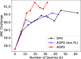
(a) ARC Challenge

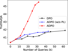
(b) TruthfulQA

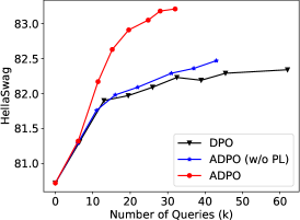
(c) HellaSwag

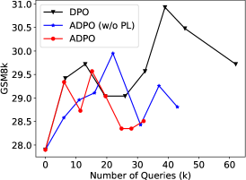
(d) GSM8k

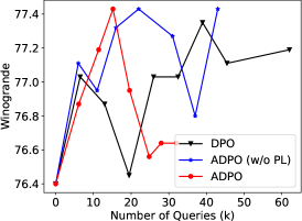
(e) Winogrande

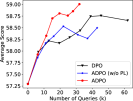
(f) Average Score

Figure 1: The test accuracy curves of DPO, DPO-AQ (w/o PL) and ADPO. The x-axis represents the number of queries, and the y-axis corresponds to the metric for the respective dataset. Compared to DPO and DPO-AQ (w/o PL), ADPO enjoys a faster performance improvement and achieves a higher performance upper bound. Additionally, we observe some instability in the training curve of GSM8k and Winogrande.

Table 3: The effect of uncertainty threshold in practice setting. We vary the value of $\Gamma$ and report the evaluation results. As $\Gamma$ increases, ADPO makes more queries, and the performance pattern gets closer to that of DPO.

$\Gamma$	Arc	TQA	WG	GSM8k	HS	MMLU	Avg	# Queries
1.0	61.01	48.41	76.64	20.39	83.35	58.89	58.115	16k
1.3	61.43	47.56	76.24	24.41	83.48	58.44	58.59	24k
1.5	61.26	45.52	76.64	28.51	83.21	58.89	59.005	32k
1.8	60.92	43.2	77.35	29.26	82.13	59.94	58.80	43k

Table 4: The effect of pseudo-labels. The numbers in parentheses represent the corresponding uncertainty threshold $\Gamma$. ADPO outperforms DPO-AQ (w/o PL) in terms of average scores.

Model	Arc	TQA	WG	GSM8k	HS	MMLU	Avg	# Queries
ADPO (w/o PL) (0.8)	60.49	41.39	77.35	29.26	82.23	60.01	58.46	38k
ADPO (w/o PL) (1.0)	60.49	41.62	77.43	28.73	82.32	60.02	58.44	40k
ADPO (w/o PL) (1.2)	60.49	41.79	77.43	28.81	82.47	59.99	58.50	43k
ADPO	61.26	45.52	76.64	28.51	83.21	58.89	59.01	32k

Query Efficiency.

To further demonstrate the query efficiency of ADPO, we plot the accuracy curves for ADPO and the baseline as the number of queries increases across all datasets, along with the average score. The curves for ARC, HellaSwag, TruthfulQA, Winogrande, GSM8k, and the average score are depicted in Figure 1. The results show that, in terms of ARC, HellaSwag, TruthfulQA and the average score, the improvement of DPO slows down after training on 20k samples. After training on 40k samples, the overall performance even begins to stagnate. In contrast, the performance of ADPO enjoys a faster improvement after training with the first 10k samples, and quickly reaches the peak with only 1/3 to 1/2 of the total queries. This suggests that ADPO can effectively select the most informative data to query the preference labels. Recall that ADPO cannot outperform DPO on Winogrande and MMLU. From Figure 1(d) and Figure 1(e), we observe an apparent training instability in both DPO and ADPO. Therefore, the failure of our method on these two datasets can be attributed to the unstable training dynamic.

7.3 Ablation Study

In this subsection, we study some important parts that might play central roles in ADPO. We first empirically study the effect of the uncertainty threshold. We also conduct experiments to demonstrate the impact of using pseudo labels in the training process.

Values of Uncertainty Threshold.

We first study the impact of different uncertainty thresholds. We vary the value of $\Gamma$ to 1.0, 1.3, 1.5, and 1.8. For each $\Gamma$, we count the preference labels used by the models and evaluate the trained models on the Open LLM Benchmark. As shown in Table 3, when the uncertainty threshold is small, with more queried preference labels, these models perform better on the TruthfulQA dataset. However, they perform poorly on datasets like GSM8k. On the other hand, when the uncertainty threshold goes larger, the models make more queries, and the performance patterns become closer to the DPO baseline. Another observation is that when $\Gamma\geq 1.5$, ADPO consistently outperforms the DPO baseline, which implies that ADPO is not very sensitive to the uncertainty threshold.

Pseudo Labels v.s. Without Pseudo Labels.

An alternative to active learning is to directly follow Algorithm 1 and simply neglect those training data with low uncertainty. Formally, we change the labels used for training from $o_{\bm{\theta}}$ to $o_{\bm{\theta}}^{\prime}$ where $o_{\bm{\theta}}^{\prime}$ is defined as follows:

$$o_{\bm{\theta}}^{\prime}(x,y^{1},y^{2})=\begin{cases}o&\text{if $U_{\bm{\theta}}(x,y^{1},y^{2})\geq\Gamma$}\\ 0&\text{if $U_{\bm{\theta}}(x,y^{1},y^{2})<\Gamma$}\end{cases}.$$

We keep the remaining part of our method the same and denote this method by ADPO (w/o PL). In this experiment, we also conduct a grid search for the uncertainty threshold $\Gamma$ and finally pick $\Gamma$ to be $0.8$, $1.0$, and $1.2$. The performances of the trained models are shown in Table 4. We plot the training curve in Figure 1. The results show that, without pseudo-labels, the performance suffers from a significant downgrade in average score compared to ADPO. The training curves further indicate that, without pseudo labels, the training dynamics are much more similar to vanilla DPO. These results show the crucial role of pseudo-labels in the active preference learning process.

8 Conclusion and Future Work

In this work, we consider query-efficient methods for aligning LLMs with human preferences. We first formulated the problem as a contextual dueling bandit. Under the linear reward and sub-optimal gap assumption, we propose an active-learning-based algorithm. Our theoretical analysis shows that our algorithm enjoys a constant regret upper bound and query complexity. We then adapt our algorithm to direct preference optimization and propose a query-efficient DPO method called ADPO. Experimental results show that ADPO outperforms DPO with only half the demand on human preference labels. Despite the good performance ADPO achieves, our theoretical analysis of APPO cannot be directly applied to ADPO. We leave the theoretical analysis of ADPO as our future work.

Appendix A Proof of Theorems in Section 5

In this section, we provide the proof of Theorem 5.1 and we first introduce several lemmas. The following lemma provides an upper bound on the query complexity and the corresponding dataset size $|\mathcal{C}_{T}|$.

Lemma A.1 (Modified from Lemma 4.5, Zhang et al., 2023).

Given a uncertainty threshold $0<\Gamma\leq 1$, if we set the regularization parameter $\lambda=B^{-2}$, then for each round $t\in[T]$, we have $|\mathcal{C}_{t}|\leq|\mathcal{C}_{T}|\leq 16d\Gamma^{-2}\log(3LB\Gamma^{-1})$.

For a finite dataset $\mathcal{C}_{T}$, the following lemma provides a upper bound for the estimation error between $\widehat{\bm{\theta}}_{t}$ and $\bm{\theta}^{*}$.

Lemma A.2.

Suppose we have $\|\bm{\theta}^{*}\|\leq B$, $\|\bm{\phi}(x,y)\|\leq L/2$. Then with probability at least $1-\delta$, for each round $t\in[T]$, we have

$$\|\bm{\theta}^{*}-\widehat{\bm{\theta}}_{t}\|_{\Sigma_{t-1}}\leq\frac{1}{\kappa_{\mu}}\cdot\big{(}\sqrt{\lambda}B+\sqrt{2d\log(\lambda+|\mathcal{C}_{T}|L^{2}/d\lambda\delta)}\big{)},$$

Based on Lemmas A.1 and A.2, the following auxiliary lemma proposes a proper choice for the uncertainty threshold $\Gamma$ and confidence radius $\beta$ in Algorithm 1.

Lemma A.3.

If we set the uncertainty threshold $\Gamma=\kappa_{\mu}\Delta/(2d\iota_{1})$ and confidence radius $\beta=\kappa_{\mu}^{-1}(1+4\sqrt{d\iota_{2}}+\sqrt{2d\iota_{3}})$, where $\iota_{1}=42\log(126LB\sqrt{d}\Delta^{-1}\kappa_{\mu}^{-1})+\sqrt{8\log(1/\delta)}$, $\iota_{2}=\log(3LB\Gamma^{-1})$ and $\iota_{3}=\log\big{(}(1+16L^{2}B^{2}\Gamma^{-2}\iota_{2})/\delta\big{)}$, then we have $2\beta\Gamma<\Delta$ and

$$\beta\geq\frac{1}{\kappa_{\mu}}\cdot\big{(}\sqrt{\lambda}B+\sqrt{2d\log(\lambda+|\mathcal{C}_{T}|L^{2}/d\lambda\delta)}\big{)}.$$

With these parameters, we now define the event $\mathcal{E}_{1}$ as

$$\mathcal{E}_{1}=\{\forall t\in[T],\|\widehat{\bm{\theta}}_{t}-\bm{\theta}^{*}\|_{\bm{\Sigma}_{t-1}^{-1}}\leq\beta\}.$$

According to Lemma A.2 and Lemma A.3, we have $\Pr(\mathcal{E}_{1})\geq 1-\delta$. Conditioned on the event $\mathcal{E}_{1}$, the following lemma suggests that our estimated discrepancy is no less than the actual discrepancy.

Lemma A.4.

On the event $\mathcal{E}_{1}$, for each round $t\in[T]$, context $x\in\mathcal{X}$ and any action $y\in\mathcal{A}$, the estimated discrepancy $\widehat{D}_{t}(x,y)$ satisfied

$$\widehat{D}_{t}(x,y)\geq D_{t}(x,y)=\langle\bm{\theta}^{*},\bm{\phi}(x,y)-\bm{\phi}_{t}^{2}\rangle.$$

On the other hand, we have

$$\widehat{D}_{t}(x,y)\leq D_{t}(x,y)+2\beta\|\bm{\phi}(x,y)-\bm{\phi}^{2}_{t}\|_{\bm{\Sigma}_{t-1}^{-1}}.$$

It is worth to notice that in Algorithm 1 (Line 13), we update the policy $\pi_{t}$ with online mirror descent and the following lemma provides the regret guarantee for this process.

Lemma A.5 (Modified from Lemma 6.2, He et al., 2022b).

For any estimated value function $\widehat{D}_{t}(x,\cdot)$, if we update the policy $\pi_{t+1}(\cdot|x)$ by the exponential rule:

$$\pi_{t+1}(\cdot|x)\propto\pi_{t}(\cdot|x)\cdot\exp\big{(}\eta\widehat{D}_{t}(x,\cdot)\big{)},$$ (A.1)

then the expected sub-optimality gap at round $T$ can be upper bounded as follows:

$$\mathbb{E}_{x\sim\mathcal{D},y\sim\pi^{*}(\cdot|x)}[\widehat{D}_{t}(x,y)]-\mathbb{E}_{x\sim\mathcal{D},y\sim\pi_{t}(\cdot|x)}[\widehat{D}_{t}(x,y)]$$

$$\quad\leq 2\eta+\eta^{-1}\mathbb{E}_{x\sim\mathcal{D}}\Big{[}\text{KL}\big{(}\pi^{*}(\cdot|x)\|\pi_{t}(\cdot|x)\big{)}-\text{KL}\big{(}\pi^{*}(\cdot|x)\|\pi_{t+1}(\cdot|x)\big{)}\Big{]}$$

With the help of these lemmas, we are now ready to prove our main theorem.

Proof of Theorem 5.1.

Now we start the regret analysis. For simplicity, for each round $t\in[T]$, we use $\bm{\phi}_{t}$ to denote $\bm{\phi}(x_{t},y_{t})$. Initially, the episodes and their corresponding regret can be decomposed into two groups based on whether episode $t$ is added to the dataset $\mathcal{C}_{T}$:

$$\text{Regret}(T) =\sum_{t=1}^{T}\langle\bm{\theta}^{*},\bm{\phi}_{t}^{*}\rangle-\langle\bm{\theta}^{*},\bm{\phi}_{t}^{1}\rangle$$

$$=\sum_{t=1}^{T}D_{t}(x_{t},y_{t}^{*})-D_{t}(x_{t},y^{1}_{t})$$

$$=\underbrace{\sum_{t\in\mathcal{C}_{T}}D_{t}(x_{t},y_{t}^{*})-D_{t}(x_{t},y^{1}_{t})}_{I_{1}}+\underbrace{\sum_{t\notin\mathcal{C}_{T}}D_{t}(x_{t},y_{t}^{*})-D_{t}(x_{t},y^{1}_{t})}_{I_{2}}$$ (A.2)

where $D_{t}(x,y)=\langle\bm{\theta}^{*},\bm{\phi}(x,y)-\bm{\phi}_{t}^{2}\rangle$ denotes the reward gap between action $y\in\mathcal{A}$ and selected action $y_{t}^{2}$ at round $t$.

Now, we bound this two term separately. For the term $I_{1}$, we have

$$I_{1} =\sum_{t\in\mathcal{C}_{T}}D_{t}(x_{t},y_{t}^{*})-D_{t}(x_{t},y^{1}_{t})$$

$$\leq\underbrace{\sum_{t\in\mathcal{C}_{T}}\widehat{D}_{t}(x_{t},y_{t}^{1})-D_{t}(x_{t},y_{t}^{1})}_{J_{1}}+\sum_{t\in\mathcal{C}_{T}}\widehat{D}_{t}(x_{t},y_{t}^{*})-\widehat{D}_{t}(x_{t},y^{1}_{t})$$

$$=J_{1}+\underbrace{\sum_{t\in\mathcal{C}_{T}}\mathbb{E}_{x_{t}\sim\mathcal{D},y\sim\pi^{*}(\cdot|x)}[\widehat{D}_{t}(x_{t},y)]-\mathbb{E}_{x_{t}\sim\mathcal{D},y\sim\pi_{t}(\cdot|x)}[\widehat{D}_{t}(x_{t},y)]}_{J_{2}}$$

$$\qquad+\underbrace{\sum_{t\in\mathcal{C}_{T}}\widehat{D}_{t}(x_{t},y_{t}^{*})-\widehat{D}_{t}(x_{t},y_{t}^{1})-\sum_{t\in\mathcal{C}_{T}}\mathbb{E}_{x_{t}\sim\mathcal{D},y\sim\pi^{*}(\cdot|x)}[\widehat{D}_{t}(x_{t},y)]-\mathbb{E}_{x_{t}\sim\mathcal{D},y\sim\pi_{t}(\cdot|x)}[\widehat{D}_{t}(x_{t},y_{t})]}_{J_{3}},$$ (A.3)

where the inequality holds due to Lemma A.4.

For the term $J_{1}$, we have

$$J_{1} =\sum_{t\in\mathcal{C}_{T}}\widehat{D}_{t}(x_{t},y_{t}^{1})-D_{t}(x_{t},y^{1}_{t})$$

$$\leq\sum_{t\in\mathcal{C}_{T}}\min\{4,2\beta\|\bm{\phi}_{t}^{1}-\bm{\phi}_{t}^{2}\|_{\bm{\Sigma}_{t-1}^{-1}}\}$$

$$\leq 4\beta\sqrt{|\mathcal{C}_{T}|\cdot\sum_{t\in\mathcal{C}_{T}}\min\{1,\|\bm{\phi}_{t}^{1}-\bm{\phi}_{t}^{2}\|_{\bm{\Sigma}_{t-1}^{-1}}^{2}\}}$$

$$\leq 8\beta\sqrt{|\mathcal{C}_{T}|d\log\bigg{(}\frac{\lambda d+|\mathcal{C}_{T}|L^{2}}{\lambda d}}\bigg{)},$$ (A.4)

where the first inequality holds due to Lemma A.4 with the fact that $-2\leq D_{t}(x_{y},y_{t}^{1})\leq 2$, the second inequality holds due to Cauchy–Schwarz inequality and the last inequality holds due to the elliptical potential lemma (Lemma C.7).

The term $J_{2}$ reflects the sub-optimality from the online mirror descent process and can be upper bounded by Lemma A.5. For simplicity, we denote $\mathcal{C}_{T}=\{t_{1},...,t_{K}\}$ where $K=|\mathcal{C}_{T}|$. Thus, we have

$$J_{2} =\sum_{k=1}^{K}\mathbb{E}_{x_{t_{k}}\sim\mathcal{D},y\sim\pi^{*}(\cdot|x)}[\widehat{D}_{t_{k}}(x_{t_{k}},y)]-\mathbb{E}_{x_{t_{k}}\sim\mathcal{D},y\sim\pi_{t_{k}}(\cdot|x)}[\widehat{D}_{t_{k}}(x_{t_{k}},y)]$$

$$\leq\sum_{k=1}^{K}\big{(}2\eta+\eta^{-1}\mathbb{E}_{x\sim\mathcal{D}}\big{[}\text{KL}(\pi^{*}(\cdot|x)\|\pi_{t_{k}}(\cdot|x))-\text{KL}(\pi^{*}(\cdot|x)\|\pi_{t_{k}+1}(\cdot|x)\big{]}\big{)}$$

$$=2\eta K+\eta^{-1}\mathbb{E}_{x\sim\mathcal{D}}\big{[}\text{KL}(\pi^{*}(\cdot|x)\|\pi_{1}(\cdot|x))-\text{KL}(\pi^{*}(\cdot|x)\|\pi_{t_{K}+1}(\cdot|x)\big{]}$$

$$\leq 2\eta K+\eta^{-1}\mathbb{E}_{x\sim\mathcal{D}}\big{[}\text{KL}(\pi^{*}(\cdot|x)\|\pi_{1}(\cdot|x))\big{]}$$

$$\leq 2\sqrt{32d\Gamma^{-2}\log(3LB\Gamma^{-1})\log|\mathcal{A}|},$$ (A.5)

where the first inequality holds due to Lemma A.5, the second equation holds due to policy $\pi$ keeps unchanged for $t\in\mathcal{C}_{T}$, the second inequality holds due to $\text{KL}(\cdot\|\cdot)\geq 0$ and the last inequality holds due to $\eta=\sqrt{\Gamma^{2}\log\mathcal{A}/\big{(}32d\log(3LB\Gamma^{-1})\big{)}}$ with the fact that $\pi_{1}$ is uniform policy.

According to Azuma-Hoeffding’s inequality (Lemma C.6), with probability at least $1-\delta$, the term $J_{3}$ can be upper bounded by

$$J_{3}\leq 2\sqrt{2|\mathcal{C}_{T}|\log(1/\delta)}.$$ (A.6)

Substituting (A), (A) and (A.6) into (A.3), we have

$$I_{1}=J_{1}+J_{2}+J_{3} \leq 8\beta\sqrt{|\mathcal{C}_{T}|d\log\bigg{(}\frac{\lambda d+|\mathcal{C}_{T}|L^{2}}{\lambda d}}\bigg{)}+2\sqrt{32d\Gamma^{-2}\log(3LB\Gamma^{-1})\log|\mathcal{A}|}+2\sqrt{2|\mathcal{C}_{T}|\log(1/\delta)}$$

$$\leq\widetilde{O}(\beta d/\Gamma)$$

$$=\widetilde{O}\bigg{(}\frac{d^{2}}{\Delta}\bigg{)}.$$ (A.7)

where the last inequality holds due to Lemma A.1.

Now, we only need to focus on the term $I_{2}$. For each round $t\notin\mathcal{C}_{T}$, we have

$$D_{t}(x_{t},y_{t}^{*})-D_{t}(x_{t},y_{t}^{1}) =\langle\bm{\theta}^{*}-\widehat{\bm{\theta}}_{t},\bm{\phi}_{t}^{*}-\bm{\phi}_{t}^{2}\rangle+\langle\widehat{\bm{\theta}}_{t},\bm{\phi}_{t}^{*}-\bm{\phi}_{t}^{2}\rangle-\langle\bm{\theta}^{*},\bm{\phi}_{t}^{1}-\bm{\phi}_{t}^{2}\rangle$$

$$\leq\beta\|\bm{\phi}_{t}^{*}-\bm{\phi}_{t}^{2}\|_{\bm{\Sigma}_{t-1}^{-1}}+\langle\widehat{\bm{\theta}}_{t},\bm{\phi}_{t}^{*}-\bm{\phi}_{t}^{2}\rangle-\langle\bm{\theta}^{*},\bm{\phi}_{t}^{1}-\bm{\phi}_{t}^{2}\rangle$$

$$\leq\beta\|\bm{\phi}_{t}^{1}-\bm{\phi}_{t}^{2}\|_{\bm{\Sigma}_{t-1}^{-1}}+\langle\widehat{\bm{\theta}}_{t},\bm{\phi}_{t}^{1}-\bm{\phi}_{t}^{2}\rangle-\langle\bm{\theta}^{*},\bm{\phi}_{t}^{1}-\bm{\phi}_{t}^{2}\rangle$$

$$\leq 2\beta\|\bm{\phi}_{t}^{1}-\bm{\phi}_{t}^{2}\|_{\bm{\Sigma}_{t-1}^{-1}},$$

where the first inequality holds due to Lemma A.4, the second inequality holds due to the selection rule of action $\bm{\phi}_{t}^{1}$ and the last inequality holds due to Lemma A.4. According to the definition of set $\mathcal{C}_{T}$ in Algorithm 1, for each round $t\notin\mathcal{C}_{T}$, we have $\|\bm{\phi}_{t}^{1}-\bm{\phi}_{t}\|_{\bm{\Sigma}_{t-1}^{-1}}\leq\Gamma$. Therefore, the sub-optimality gap at round $t$ is upper bounded by

$$2\beta\|\bm{\phi}_{t}^{1}-\bm{\phi}_{t}\|_{\bm{\Sigma}_{t-1}^{-1}}\leq 2\beta\Gamma<\Delta,$$

where the second inequality holds due to Lemma A.3. According to the minimal sub-optimality assumption (Assumption 3.4), this indicates that the regret yielded in round $t\notin\mathcal{C}_{T}$ is 0. Summing up over $t\notin\mathcal{C}_{T}$, we have

$$I_{2}=\sum_{t\in{\mathcal{T}}_{t}}D_{t}(x_{t},y_{t}^{*})-D_{t}(x_{t},y_{t}^{1})=0.$$ (A.8)

Combining the results in (A.7) and (A.8), we complete the proof of Theorem 5.1. ∎

Appendix B Proof of Lemmas in Appendix A

In this section, we provide the proofs of the lemmas in Appendix A.

B.1 Proof of Lemma A.1

Proof of Lemma A.1.

The proof follows the proof in Zhang et al. (2023). Here we fix the round $t$ to be $T$ in the proof and only provide the upper bound of $\mathcal{C}_{T}$ due to the fact that $\mathcal{C}_{t}$ is monotonically increasing w.r.t. the round $t$. For all selected episode $t\in\mathcal{C}_{T}$, since we have $\|\bm{\phi}_{t}^{1}-\bm{\phi}_{t}^{2}\|_{\bm{\Sigma}_{t-1}^{-1}}\geq\Gamma$, the summation of the bonuses over all the selected episode $t\in\mathcal{C}_{T}$ is lower bounded by

$$\sum_{t\in\mathcal{C}_{T}}\min\left\{1,\|\bm{\phi}_{t}^{1}-\bm{\phi}_{t}^{2}\|_{\bm{\Sigma}_{t-1}^{-1}}^{2}\right\}\geq|\mathcal{C}_{T}|\min\{1,\Gamma^{2}\}=|\mathcal{C}_{T}|\Gamma^{2},$$ (B.1)

where the last equation holds due to $0\leq\Gamma\leq 1$. On the other hand, according to Lemma C.3, the summation is upper bounded by:

$$\sum_{t\in\mathcal{C}_{T}}\min\left\{1,\|\bm{\phi}_{t}^{1}-\bm{\phi}_{t}^{2}\|_{\bm{\Sigma}_{t-1}^{-1}}^{2}\right\}\leq 2d\log\left(\frac{\lambda d+|\mathcal{C}_{T}|L^{2}}{\lambda d}\right).$$ (B.2)

Combining (B.1) and (B.2), we know that the total number of the selected data points $|\mathcal{C}_{T}|$ satisfies the following inequality:

$$\Gamma^{2}|\mathcal{C}_{T}|\leq 2d\log\left(\frac{\lambda d+|\mathcal{C}_{T}|L^{2}}{\lambda d}\right).$$

For simplicity, we reorganized the result as follows:

$$\frac{\Gamma^{2}|\mathcal{C}_{T}|}{2d}\leq\log\left(1+\frac{2L^{2}}{\Gamma^{2}\lambda}\frac{\Gamma^{2}|\mathcal{C}_{T}|}{2d}\right).$$ (B.3)

Notice that $\lambda=B^{-2}$ and $2L^{2}B^{2}\geq 2\geq\Gamma^{2}$, therefore, if $|\mathcal{C}_{T}|$ is too large such that

$$\frac{\Gamma^{2}|\mathcal{C}_{T}|}{2d}>4\log\left(\frac{4L^{2}B^{2}}{\Gamma^{2}}\right)+1\geq 4\log\left(\frac{4L^{2}B^{2}}{\Gamma^{2}}\right)+\frac{\Gamma^{2}}{2L^{2}B^{2}},$$

then according to Lemma C.1, (B.3) will not hold. Thus the necessary condition for (B.3) to hold is:

$$\frac{\Gamma^{2}|\mathcal{C}_{T}|}{2d}\leq 4\log\left(\frac{4L^{2}B^{2}}{\Gamma^{2}}\right)+1=8\log\left(\frac{2LB}{\Gamma}\right)+\log(e)=8\log\left(\frac{2LBe^{\frac{1}{8}}}{\Gamma}\right)<8\log\left(\frac{3LB}{\Gamma}\right).$$

Applying basic calculus, we obtain the claimed bound for $|\mathcal{C}_{T}|$ and thus complete the proof of Lemma A.1. ∎

B.2 Proof of Lemma A.2

Proof of Lemma A.2.

This proof follows the proof in Di et al. (2023). For each round $t\in[T]$, we define the following auxiliary quantities:

$$G_{t}(\bm{\theta})=\lambda\bm{\theta}+\sum_{\tau\in\mathcal{C}_{t-1}}\Big{[}\mu\big{(}(\bm{\phi}_{\tau}^{1}-\bm{\phi}_{\tau}^{2})^{\top}\bm{\theta}\big{)}-\mu\big{(}(\bm{\phi}_{\tau}^{1}-\bm{\phi}_{\tau}^{2})^{\top}\bm{\theta}^{*}\big{)}\Big{]}(\bm{\phi}_{\tau}^{1}-\bm{\phi}_{\tau}^{2})$$

$$\epsilon_{t}=o_{t}-\mu\big{(}(\bm{\phi}_{t}^{1}-\bm{\phi}_{t}^{2})^{\top}\bm{\theta}^{*}\big{)}$$

$$Z_{t}=\sum_{\tau\in\mathcal{C}_{t-1}}\epsilon_{\tau}(\bm{\phi}_{\tau}^{1}-\bm{\phi}_{\tau}^{2}).$$

By defining $\widehat{\bm{\theta}}_{t}$ as the solution to (4.1), we plug the equation into the definition of $G_{t}$ and we have

$$G_{t}(\widehat{\bm{\theta}}_{t}) =\lambda\widehat{\bm{\theta}}_{t}+\sum_{\tau\in\mathcal{C}_{t-1}}\Big{[}\mu\big{(}(\bm{\phi}_{\tau}^{1}-\bm{\phi}_{\tau}^{2})^{\top}\widehat{\bm{\theta}}_{t})-o_{\tau}+o_{\tau}-\mu\big{(}(\bm{\phi}_{\tau}^{1}-\bm{\phi}_{\tau}^{2})^{\top}\bm{\theta}^{*}\big{)}\Big{]}(\bm{\phi}_{\tau}^{1}-\bm{\phi}_{\tau}^{2})$$

$$=\lambda\widehat{\bm{\theta}}_{t}+\sum_{\tau\in\mathcal{C}_{t-1}}\Big{[}\mu\big{(}(\bm{\phi}_{\tau}^{1}-\bm{\phi}_{\tau}^{2})^{\top}\widehat{\bm{\theta}}_{t})-o_{\tau}\Big{]}(\bm{\phi}_{\tau}^{1}-\bm{\phi}_{\tau}^{2})+\sum_{\tau\in\mathcal{C}_{t-1}}\Big{[}o_{\tau}-\mu\big{(}(\bm{\phi}_{\tau}^{1}-\bm{\phi}_{\tau}^{2})^{\top}\bm{\theta}^{*}\big{)}\Big{]}(\bm{\phi}_{\tau}^{1}-\bm{\phi}_{\tau}^{2})$$

$$=Z_{t}.$$

Therefore, we have that

$$G_{t}(\widehat{\bm{\theta}}_{t})-G_{t}(\bm{\theta}^{*})=Z_{t}-G_{t}(\bm{\theta}^{*})=Z_{t}-\lambda\bm{\theta}^{*}.$$

On the other hand, applying Taylor’s expansion, there exists $\alpha\in[0,1]$ and $\widetilde{\bm{\theta}}_{t}=\alpha\widehat{\bm{\theta}}_{t}+(1-\alpha)\bm{\theta}^{*}$, such that the following equation holds:

$$G_{t}(\widehat{\bm{\theta}}_{t})-G_{t}(\bm{\theta}^{*}) =\lambda(\widehat{\bm{\theta}}_{t}-\bm{\theta}^{*})+\sum_{\tau\in\mathcal{C}_{t-1}}\Big{[}\mu\big{(}(\bm{\phi}_{\tau}^{1}-\bm{\phi}_{\tau}^{2})^{\top}\bm{\theta}\big{)}-\mu\big{(}(\bm{\phi}_{\tau}^{1}-\bm{\phi}_{\tau}^{2})^{\top}\bm{\theta}^{*}\big{)}\Big{]}(\bm{\phi}_{\tau}^{1}-\bm{\phi}_{\tau}^{2})$$

$$=\Big{[}\lambda\mathbf{I}+\sum_{\tau\in\mathcal{C}_{t-1}}\mu^{\prime}\big{(}(\bm{\phi}_{\tau}^{1}-\bm{\phi}_{\tau}^{2})^{\top}\widetilde{\bm{\theta}}_{t}\big{)}(\bm{\phi}_{\tau}^{1}-\bm{\phi}_{\tau}^{2})(\bm{\phi}_{\tau}^{1}-\bm{\phi}_{\tau}^{2})^{\top}\Big{]}(\widehat{\bm{\theta}}_{t}-\bm{\theta}^{*})$$

$$=F(\widetilde{\bm{\theta}}_{t})(\widehat{\bm{\theta}}_{t}-\bm{\theta}^{*}),$$

where we define $F(\widetilde{\bm{\theta}}_{t})=\lambda\mathbf{I}+\sum_{\tau\in\mathcal{C}_{t-1}}\mu^{\prime}\big{(}(\bm{\phi}_{\tau}^{1}-\bm{\phi}_{\tau}^{2})^{\top}\widetilde{\bm{\theta}}_{t}\big{)}(\bm{\phi}_{\tau}^{1}-\bm{\phi}_{\tau}^{2})(\bm{\phi}_{\tau}^{1}-\bm{\phi}_{\tau}^{2})^{\top}$. Thus, we have:

$$\|\widehat{\bm{\theta}}_{t}-\bm{\theta}^{*}\|^{2}_{\bm{\Sigma}_{t-1}} =(Z_{t}-\lambda\bm{\theta}^{*})^{\top}F(\widetilde{\bm{\theta}}_{t})^{-1}\bm{\Sigma}_{t-1}F(\widetilde{\bm{\theta}}_{t})^{-1}(Z_{t}-\lambda\bm{\theta}^{*})$$

$$\leq\frac{1}{\kappa_{\mu}^{2}}(Z_{t}-\lambda\bm{\theta}^{*})^{\top}\bm{\Sigma}_{t-1}^{-1}(Z_{t}-\lambda\bm{\theta}^{*})$$

$$=\frac{1}{\kappa_{\mu}^{2}}\|Z_{t}-\lambda\bm{\theta}^{*}\|_{\bm{\Sigma}_{t-1}^{-1}}^{2}$$

where the inequality holds due to $F(\widetilde{\bm{\theta}}_{t})\succeq\kappa_{\mu}\widehat{\bm{\Sigma}}_{t-1}$. Now we have:

$$\|\widehat{\bm{\theta}}_{t}-\bm{\theta}^{*}\|_{\bm{\Sigma}_{t-1}} \leq\frac{1}{\kappa_{\mu}}\|Z_{t}-\lambda\bm{\theta}^{*}\|_{\bm{\Sigma}_{t-1}^{-1}}$$

$$\leq\frac{1}{\kappa_{\mu}}\big{(}\|Z_{t}\|_{\bm{\Sigma}_{t-1}^{-1}}+\|\lambda\bm{\theta}^{*}\|_{\bm{\Sigma}_{t-1}^{-1}}\big{)}$$

$$\leq\frac{1}{\kappa_{\mu}}\big{(}\|Z_{t}\|_{\bm{\Sigma}_{t-1}^{-1}}+\sqrt{\lambda}B\big{)},$$

where the second inequality holds due to triangle inequality and last inequality holds due to $\bm{\Sigma}_{t-1}\succeq\lambda\mathbf{I}$. Now we only need to bound $\|Z_{t}\|_{\bm{\Sigma}_{t-1}^{-1}}$.

According to Lemma C.2, with probability at least $1-\delta$, we have

$$\|Z_{t}\|_{\bm{\Sigma}_{t-1}^{-1}}\leq\sqrt{2\log\bigg{(}\frac{\sqrt{\det(\bm{\Sigma}_{t-1})}}{\sqrt{\det(\bm{\Sigma}_{0})}\delta}\bigg{)}}\leq\sqrt{2\log\bigg{(}\frac{\det(\bm{\Sigma}_{t-1})}{\lambda^{d}\delta}\bigg{)}}\leq\sqrt{2d\log\bigg{(}\frac{\lambda+|\mathcal{C}_{t}|L^{2}/d}{\lambda^{d}\delta}\bigg{)}}$$

where the first inequality holds due to Lemma C.2 and the last inequality holds due to Lemma C.5. Now we combine the two term and have

$$\|\widehat{\bm{\theta}}_{t}-\bm{\theta}^{*}\|_{\bm{\Sigma}_{t-1}}\leq\frac{1}{\kappa_{\mu}}\Bigg{(}\sqrt{\lambda}B+\sqrt{2d\log\bigg{(}\frac{\lambda+|\mathcal{C}_{t}|L^{2}/d}{\lambda^{d}\delta}\bigg{)}}\Bigg{)},$$

which concludes our statement. ∎

B.3 Proof of Lemma A.3

Proof of Lemma A.3.

This proof follows the proof in Zhang et al. (2023). First, we recall that $\Gamma=\Delta\kappa_{\mu}/2d\iota_{1}$ and $\beta=\kappa_{\mu}^{-1}(1+4\sqrt{d\iota_{2}}+\sqrt{2d\iota_{3}})$. We will first demonstrate that the selection of $\beta$ satisfy the requirement in Lemma A.3. Recalling that $\lambda=B^{-2}$, through basic calculation, we have

$$\kappa_{\mu}\beta \geq 1+\sqrt{2d\log\big{(}(1+L^{2}B^{2}16d\Gamma^{-2}\iota_{2})/d\delta\big{)}}$$

$$\geq 1+\sqrt{2d\log\big{(}(1+L^{2}B^{2}|\mathcal{C}_{T}|)/d\delta\big{)}}$$

$$=\sqrt{\lambda}B+\sqrt{2d\log(\lambda+|\mathcal{C}_{T}|L^{2}/d\lambda\delta)},$$

where the first inequality holds by neglecting the positive term $4\sqrt{d\iota_{2}}$ and $d\geq 1$, the second inequality holds due to Lemma A.1 and the last equation holds by plugging in $\lambda=B^{-2}$. Now we come to the second statement. First, by basic computation, we have

$$\sqrt{2\iota_{3}}\leq\sqrt{2\log((1+16L^{2}B^{2}\Gamma^{-2}\iota_{2})}+\sqrt{2\log(1/\delta))}.$$

Notice that we have $L\geq 1$, $B\geq 1$, and $\Gamma\leq 1$, which further implies that $LB\Gamma^{-1}\geq 1$, leading to

$$2+4\sqrt{\iota_{2}}\leq 6\iota_{2},\quad\sqrt{2\log((1+16L^{2}B^{2}\Gamma^{-2}\iota_{2})}\leq 3\iota_{2}.$$

Therefore, we have:

$$2+4\sqrt{\iota_{2}}+\sqrt{2\iota_{3}} \leq 9\iota_{2}+2\sqrt{\log(1/\delta)}$$

$$\leq 9\log(6LB\sqrt{d}\Delta^{-1}\kappa_{\mu}^{-1}\iota_{1})+2\sqrt{\log(1/\delta)}.$$

By Lemma C.1, we can identify the sufficient condition for the following inequality

$$(6LB\sqrt{d}\Delta^{-1}\kappa_{\mu}^{-1})\iota_{1}\geq 9(6LB\sqrt{d}\Delta^{-1}\kappa_{\mu}^{-1})\log(6LB\sqrt{d}\Delta^{-1}\kappa_{\mu}^{-1}\iota_{1})+2(6LB\sqrt{d}\Delta^{-1}\kappa_{\mu}^{-1})\sqrt{\log(1/\delta)}$$ (B.4)

is that

$$\iota_{1}\geq 36\log(108LB\sqrt{d}\Delta^{-1}\kappa_{mu}^{-1})+\sqrt{8\log(1/\delta)},$$

which naturally holds due to our definition of $\iota_{1}$. Eliminating the $6LB\sqrt{d}\Delta^{-1}\kappa_{\mu}^{-1}$ term in (B.4) yields that

$$\iota_{1}\geq 2+4\sqrt{\iota_{2}}+\sqrt{2\iota_{3}},$$

which implies that

$$2\beta\Gamma=\frac{\Delta\kappa_{\mu}}{2\sqrt{d}\iota_{1}}\frac{1}{\kappa_{\mu}}(1+2\sqrt{d\iota_{2}}+\sqrt{2\iota_{3}})<\Delta.$$

Thus, we complete the proof of Lemma A.3. ∎

B.4 Proof of Lemma A.4

Proof of Lemma A.4.

For each context $x\in\mathcal{X}$ and action $y\in\mathcal{A}$, we have

$$|D_{t}(x,y)-\langle\widehat{\bm{\theta}}_{t},\bm{\phi}(x,y)-\bm{\phi}_{t}^{2}\rangle| =|\langle\widehat{\bm{\theta}}_{t}-\bm{\theta}^{*},\bm{\phi}(x,y)-\bm{\phi}_{t}^{2}\rangle|$$

$$\leq\|\widehat{\bm{\theta}}_{t}-\bm{\theta}^{*}\|_{\bm{\Sigma}_{t-1}^{-1}}\cdot\|\bm{\phi}(x,y)-\bm{\phi}_{t}^{2}\|_{\bm{\Sigma}_{t-1}}$$

$$\leq\beta\|\bm{\phi}(x,y)-\bm{\phi}_{t}^{2}\|_{\bm{\Sigma}_{t-1}},$$ (B.5)

where the first inequality holds due to Cauchy–Schwarz inequality and the second inequality holds due to event $\mathcal{E}_{1}$. Therefore, we have

$$\langle\widehat{\bm{\theta}}_{t},\bm{\phi}(x,y)-\bm{\phi}_{t}^{2}\rangle+\beta\|\bm{\phi}(x,y)-\bm{\phi}_{t}^{2}\|_{\bm{\Sigma}_{t-1}}\geq D_{t}(x,y),$$

where the first inequality holds due to (B.5). In addition, we have $D_{t}(x,y)=\langle\bm{\theta}^{*},\bm{\phi}(x,y)-\bm{\phi}_{t}^{2}\rangle\leq 2$. Combing these two results, we have

$$\widehat{D}_{t}(x,y)=\min\{\langle\widehat{\bm{\theta}}_{t},\bm{\phi}(x,y)-\bm{\phi}_{t}^{2}\rangle+\beta\|\bm{\phi}(x,y)-\bm{\phi}_{t}^{2}\|_{\bm{\Sigma}_{t-1}},2\}\geq D_{t}(x,y).$$

On the other hand, we have

$$\widehat{D}_{t}(x,y)\leq\langle\widehat{\bm{\theta}}_{t},\bm{\phi}(x,y)-\bm{\phi}_{t}^{2}\rangle+\beta\|\bm{\phi}(x,y)-\bm{\phi}_{t}^{2}\|_{\bm{\Sigma}_{t-1}}\leq D_{t}(x,y)+2\beta\|\bm{\phi}(x,y)-\bm{\phi}_{t}^{2}\|_{\bm{\Sigma}_{t-1}},$$

where the first inequality holds due to the definition of $\widehat{D}_{t}(x,y)$ and the second inequality holds due to (B.5). Thus, we complete the proof of Lemma A.4. ∎

B.5 Proof of Lemma A.5

Proof of Lemma A.5.

The proof follows the approach in He et al. (2022b). Recall that we assume the policy is updated in round $t$ according to the update rule (A.1), for all contexts $x\in\mathcal{X}$. Thus, we have:

$$\exp\big{\{}\eta\widehat{D}_{t}(x,y)\big{\}} =\frac{\pi_{t}(y|x)\exp\big{\{}\eta\widehat{D}_{t}(x,y)\big{\}}}{\pi_{t}(y|x)}=\frac{\rho\pi_{t+1}(y|x)}{\pi_{t}(y|x)},$$ (B.6)

where $\rho=\sum_{y\in\mathcal{A}}\pi_{t}(y|x)\exp\big{\{}\eta\widehat{D}_{t}(x,y)\big{\}}$ is the regularization term that is the same for all actions $y\in\mathcal{A}$. Therefore, we have

$$\sum_{y\in\mathcal{A}}\eta\widehat{D}_{t}(x,y)\big{(}\pi^{*}(y|x)-\pi_{t+1}(y|x)\big{)}$$

$$=\sum_{y\in\mathcal{A}}\big{(}\log\rho+\log\pi_{t+1}(y|x)-\log\pi_{t}(y|x)\big{)}\big{(}\pi^{*}(y|x)-\pi_{t+1}(y|x)\big{)}$$

$$=\sum_{y\in\mathcal{A}}\pi^{*}(y|x)\big{(}\log\pi_{t+1}(y|x)-\log\pi_{t}(y|x)\big{)}-\pi_{t+1}(y|x)\big{(}\log\pi_{t+1}(y|x)-\log\pi_{t}(y|x)\big{)}$$

$$=\sum_{y\in\mathcal{A}}\pi^{*}(y|x)\big{(}\log\pi^{*}(y|x)-\log\pi_{t}(y|x)\big{)}+\sum_{y\in\mathcal{A}}\pi^{*}(y|x)\big{(}\log\pi_{t+1}(y|x)-\log\pi^{*}(y|x)\big{)}$$

$$\qquad-\sum_{y\in\mathcal{A}}\pi_{t+1}(y|x)\big{(}\log\pi_{t+1}(y|x)-\log\pi_{t}(y|x)\big{)}$$

$$=\text{KL}\big{(}\pi^{*}(\cdot|x)\|\pi_{t}(\cdot|x)\big{)}-\text{KL}\big{(}\pi^{*}(\cdot|x)\|\pi_{t+1}(\cdot|x)\big{)}-\text{KL}\big{(}\pi_{t+1}(\cdot|x)\|\pi_{t}(\cdot|x)\big{)},$$ (B.7)

where the first equation holds due to (B.6) and the second equation holds due to $\sum_{y\in\mathcal{A}}\big{(}\pi^{*}(y|x)-\pi_{t+1}(y|x)\big{)}=0$. Consequently, we have

$$\mathbb{E}_{y\sim\pi^{*}(\cdot|x)}\big{[}\widehat{D}_{t}(x,y)\big{]}-\mathbb{E}_{y\sim\pi_{t}(\cdot|x)}\big{[}\widehat{D}_{t}(x,y)\big{]}$$

$$=\sum_{y\in\mathcal{A}}\widehat{D}_{t}(x,y)\big{(}\pi^{*}(y|x)-\pi_{t}(y|x)\big{)}$$

$$=\sum_{y\in\mathcal{A}}\widehat{D}_{t}(x,y)\big{(}\pi^{*}(y|x)-\pi_{t+1}(y|x)\big{)}+\sum_{y\in\mathcal{A}}\widehat{D}_{t}(x,y)\big{(}\pi_{t+1}(y|x)-\pi_{t}(y|x)\big{)}$$

$$\leq\sum_{y\in\mathcal{A}}\widehat{D}_{t}(x,y)\big{(}\pi^{*}(y|x)-\pi_{t+1}(y|x)\big{)}+2\big{\|}\pi_{t+1}(\cdot|x)-\pi_{t}(\cdot|x)\big{\|}_{1}$$

$$=\eta^{-1}\Big{(}\text{KL}\big{(}\pi^{*}(\cdot|x)\|\pi_{t}(\cdot|x)\big{)}-\text{KL}\big{(}\pi^{*}(\cdot|x)\|\pi_{t+1}(\cdot|x)\big{)}-\text{KL}\big{(}\pi_{t+1}(\cdot|x)\|\pi_{t}(\cdot|x)\big{)}\Big{)}$$

$$\qquad+2\big{\|}\pi_{t+1}(\cdot|x)-\pi_{t}(\cdot|x)\big{\|}_{1}$$

$$\leq\eta^{-1}\Big{(}\text{KL}\big{(}\pi^{*}(\cdot|x)\|\pi_{t}(\cdot|x)\big{)}-\text{KL}\big{(}\pi^{*}(\cdot|x)\|\pi_{t+1}(\cdot|x)\big{)}\Big{)}$$

$$\qquad+2\big{\|}\pi_{t+1}(\cdot|x)-\pi_{t}(\cdot|x)\big{\|}_{1}-\frac{\big{\|}\pi_{t+1}(\cdot|x)-\pi_{t}(\cdot|x)\big{\|}_{1}^{2}}{2\eta}$$

$$\leq 2\eta+\eta^{-1}\Big{(}\text{KL}\big{(}\pi^{*}(\cdot|x)\|\pi_{t}(\cdot|x)\big{)}-\text{KL}\big{(}\pi^{*}(\cdot|x)\|\pi_{t+1}(\cdot|x)\big{)}\Big{)},$$ (B.8)

where the first inequality holds due to the fact that $0\leq\widehat{D}_{t}(x,y)\leq 2$, the second inequality holds due to Pinsker’s inequality and the last inequality holds due to the fact that $ax-bx^{2}\leq a^{2}/4b$. Finally, taking expectation over $x\sim\mathcal{D}$ finishes the proof. ∎

Appendix C Auxiliary Lemmas

Lemma C.1 (Lemma A.2, Shalev-Shwartz and Ben-David, 2014).

Let $a\geq 1$ and $b\geq 0$, then $x\geq 4a\log(2a)+2b$ results in $x\geq a\log x+b$.

Lemma C.2 (Theorem 1, Abbasi-Yadkori et al., 2011).

Let $\{\mathcal{F}_{t}\}_{t=0}^{\infty}$ be a filtration. Let $\{\epsilon_{t}\}_{t=1}^{\infty}$ be a real-valued stochastic process such that $\epsilon_{t}$ is $\mathcal{F}_{t}$-measurable and $\epsilon_{t}$ is conditionally $R$-sub-Gaussian for some $R\geq 0$. Let $\{\bm{\phi}_{t}\}_{t=1}^{\infty}$ be an $\mathbb{R}^{d}$-valued stochastic process such that $\bm{\phi}_{t}$ is $\mathcal{F}_{t-1}$ measurable and $\|\bm{\phi}_{t}\|_{2}\leq L$ for all $t$. For any $t\geq 0$, define $\mathbf{U}_{t}=\lambda\mathbf{I}+\sum_{i=1}^{t}\bm{\phi}_{i}\bm{\phi}_{i}^{\top}$. Then for any $\delta>0$, with probability at least $1-\delta$, for all $t\geq 0$, we have

$$\left\|\sum_{i=1}^{t}\bm{\phi}_{i}\epsilon_{i}\right\|_{\mathbf{U}_{t}^{-1}}^{2}\leq 2R^{2}\log\left(\frac{\sqrt{\det(\mathbf{U}_{t})}}{\sqrt{\det(\mathbf{U}_{0})}\delta}\right).$$

Lemma C.3 (Lemma 11, Abbasi-Yadkori et al. 2011).

Let $\{\bm{\phi}_{i}\}_{i=1}^{t}$ be a sequence in $\mathbb{R}^{d}$, define $\mathbf{U}_{i}=\lambda\mathbf{I}+\sum_{i=1}^{t}\bm{\phi}_{i}\bm{\phi}_{i}^{\top}$, then

$$\sum_{i=1}^{t}\min\left\{1,\|\bm{\phi}_{i}\|_{\mathbf{U}_{i-1}^{-1}}^{2}\right\}\leq 2d\log\left(\frac{\lambda d+tL^{2}}{\lambda d}\right).$$

The following auxiliary lemma and its corollary are useful

Lemma C.4 (Lemma A.2, Shalev-Shwartz and Ben-David 2014).

Let $a\geq 1$ and $b>0$. Then $x\geq 4a\log(2a)+2b$ yields $x\geq a\log(x)+b$.

Lemma C.5 (Lemma C.7, Zhang et al., 2023).

Suppose sequence $\{\mathbf{x}_{i}\}_{i=1}^{t}\subset\mathbb{R}^{d}$ and for any $i\leq t$, $\|\mathbf{x}_{i}\|_{2}\leq L$. For any index subset $\mathcal{C}\subseteq[t]$, define $\mathbf{U}=\lambda\mathbf{I}+\sum_{i\in\mathcal{C}}\mathbf{x}_{i}\mathbf{x}_{i}^{\top}$ for some $\lambda>0$, then $\det(\mathbf{U})\leq(\lambda+|\mathcal{C}|L^{2}/d)^{d}$.

Lemma C.6 (Azuma–Hoeffding inequality, Cesa-Bianchi and Lugosi 2006).

Let $\{x_{i}\}_{i=1}^{n}$ be a martingale difference sequence with respect to a filtration $\{\mathcal{G}_{i}\}$ satisfying $|x_{i}|\leq M$ for some constant $M$, $x_{i}$ is $\mathcal{G}_{i+1}$-measurable, $\mathbb{E}[x_{i}|\mathcal{G}_{i}]=0$. Then for any $0<\delta<1$, with probability at least $1-\delta$, we have

$$\sum_{i=1}^{n}x_{i}\leq M\sqrt{2n\log(1/\delta)}.$$

Lemma C.7 (Lemma 11 in Abbasi-Yadkori et al. (2011)).

Let $\{\bm{\phi}_{t}\}_{t=1}^{+\infty}$ be a sequence in $\mathbb{R}^{d}$, $\mathbf{U}$ a $d\times d$ positive definite matrix and define $\mathbf{U}_{t}=\mathbf{U}+\sum_{i=1}^{t}\bm{\phi}_{i}^{\top}\bm{\phi}_{i}$. If $\|\bm{\phi}_{i}\|_{2}\leq L$ and $\lambda_{\min}(\mathbf{U})\geq\max(1,L^{2}),$ then we have

$$\sum_{i=1}^{t}\bm{\phi}_{i}^{\top}(\mathbf{U}_{i-1})^{-1}\bm{\phi}_{i}\leq 2\log\bigg{(}\frac{\det{\mathbf{U}_{t}}}{\det{\mathbf{U}}}\bigg{)}.$$

References

- Abbasi-Yadkori et al. (2011) Abbasi-Yadkori, Y., Pál, D. and Szepesvári, C. (2011). Improved algorithms for linear stochastic bandits. Advances in neural information processing systems 24.
- Achiam et al. (2023) Achiam, J., Adler, S., Agarwal, S., Ahmad, L., Akkaya, I., Aleman, F. L., Almeida, D., Altenschmidt, J., Altman, S., Anadkat, S. et al. (2023). Gpt-4 technical report. arXiv preprint arXiv:2303.08774 .
- Bai et al. (2022) Bai, Y., Jones, A., Ndousse, K., Askell, A., Chen, A., DasSarma, N., Drain, D., Fort, S., Ganguli, D., Henighan, T. et al. (2022). Training a helpful and harmless assistant with reinforcement learning from human feedback. arXiv preprint arXiv:2204.05862 .
- Balcan et al. (2006) Balcan, M.-F., Beygelzimer, A. and Langford, J. (2006). Agnostic active learning. In Proceedings of the 23rd international conference on Machine learning.
- Balcan et al. (2007) Balcan, M.-F., Broder, A. and Zhang, T. (2007). Margin based active learning. In International Conference on Computational Learning Theory. Springer.
- Balsubramani et al. (2016) Balsubramani, A., Karnin, Z., Schapire, R. E. and Zoghi, M. (2016). Instance-dependent regret bounds for dueling bandits. In Conference on Learning Theory. PMLR.
- Beeching et al. (2023) Beeching, E., Fourrier, C., Habib, N., Han, S., Lambert, N., Rajani, N., Sanseviero, O., Tunstall, L. and Wolf, T. (2023). Open llm leaderboard. https://huggingface.co/spaces/HuggingFaceH4/open_llm_leaderboard.
- Bengs et al. (2022) Bengs, V., Saha, A. and Hüllermeier, E. (2022). Stochastic contextual dueling bandits under linear stochastic transitivity models. In International Conference on Machine Learning. PMLR.
- Bradley and Terry (1952) Bradley, R. A. and Terry, M. E. (1952). Rank analysis of incomplete block designs: I. the method of paired comparisons. Biometrika 39 324–345.
- Cai et al. (2020) Cai, Q., Yang, Z., Jin, C. and Wang, Z. (2020). Provably efficient exploration in policy optimization. In International Conference on Machine Learning. PMLR.
- Casper et al. (2023) Casper, S., Davies, X., Shi, C., Gilbert, T. K., Scheurer, J., Rando, J., Freedman, R., Korbak, T., Lindner, D., Freire, P. et al. (2023). Open problems and fundamental limitations of reinforcement learning from human feedback. arXiv preprint arXiv:2307.15217 .
- Cesa-Bianchi et al. (2009) Cesa-Bianchi, N., Gentile, C. and Orabona, F. (2009). Robust bounds for classification via selective sampling. In Proceedings of the 26th annual international conference on machine learning.
- Cesa-Bianchi et al. (2006) Cesa-Bianchi, N., Gentile, C., Zaniboni, L. and Warmuth, M. (2006). Worst-case analysis of selective sampling for linear classification. Journal of Machine Learning Research 7.
- Cesa-Bianchi and Lugosi (2006) Cesa-Bianchi, N. and Lugosi, G. (2006). Prediction, learning, and games. Cambridge university press.
- Cesa-Bianchi et al. (2005) Cesa-Bianchi, N., Lugosi, G. and Stoltz, G. (2005). Minimizing regret with label efficient prediction. IEEE Transactions on Information Theory 51 2152–2162.
- Chiang et al. (2023) Chiang, W.-L., Li, Z., Lin, Z., Sheng, Y., Wu, Z., Zhang, H., Zheng, L., Zhuang, S., Zhuang, Y., Gonzalez, J. E., Stoica, I. and Xing, E. P. (2023). Vicuna: An open-source chatbot impressing gpt-4 with 90%* chatgpt quality.
- Christiano et al. (2017) Christiano, P. F., Leike, J., Brown, T., Martic, M., Legg, S. and Amodei, D. (2017). Deep reinforcement learning from human preferences. Advances in neural information processing systems 30.
- Citovsky et al. (2021) Citovsky, G., DeSalvo, G., Gentile, C., Karydas, L., Rajagopalan, A., Rostamizadeh, A. and Kumar, S. (2021). Batch active learning at scale. Advances in Neural Information Processing Systems 34 11933–11944.
- Clark et al. (2018) Clark, P., Cowhey, I., Etzioni, O., Khot, T., Sabharwal, A., Schoenick, C. and Tafjord, O. (2018). Think you have solved question answering? try arc, the ai2 reasoning challenge. arXiv preprint arXiv:1803.05457 .
- Cobbe et al. (2021) Cobbe, K., Kosaraju, V., Bavarian, M., Chen, M., Jun, H., Kaiser, L., Plappert, M., Tworek, J., Hilton, J., Nakano, R. et al. (2021). Training verifiers to solve math word problems. arXiv preprint arXiv:2110.14168 .
- Dasgupta (2005) Dasgupta, S. (2005). Coarse sample complexity bounds for active learning. Advances in neural information processing systems 18.
- Dasgupta et al. (2005) Dasgupta, S., Kalai, A. T. and Monteleoni, C. (2005). Analysis of perceptron-based active learning. In International conference on computational learning theory. Springer.
- Di et al. (2023) Di, Q., Jin, T., Wu, Y., Zhao, H., Farnoud, F. and Gu, Q. (2023). Variance-aware regret bounds for stochastic contextual dueling bandits. arXiv preprint arXiv:2310.00968 .
- Ding et al. (2023) Ding, N., Chen, Y., Xu, B., Qin, Y., Zheng, Z., Hu, S., Liu, Z., Sun, M. and Zhou, B. (2023). Enhancing chat language models by scaling high-quality instructional conversations. arXiv preprint arXiv:2305.14233 .
- Dudík et al. (2015) Dudík, M., Hofmann, K., Schapire, R. E., Slivkins, A. and Zoghi, M. (2015). Contextual dueling bandits. ArXiv abs/1502.06362.
- Falahatgar et al. (2018) Falahatgar, M., Jain, A., Orlitsky, A., Pichapati, V. and Ravindrakumar, V. (2018). The limits of maxing, ranking, and preference learning. In International conference on machine learning. PMLR.
- Falahatgar et al. (2017) Falahatgar, M., Orlitsky, A., Pichapati, V. and Suresh, A. T. (2017). Maximum selection and ranking under noisy comparisons. In International Conference on Machine Learning. PMLR.
- Filippi et al. (2010) Filippi, S., Cappe, O., Garivier, A. and Szepesvári, C. (2010). Parametric bandits: The generalized linear case. Advances in Neural Information Processing Systems 23.
- Gao et al. (2023a) Gao, J., Zhao, H., Yu, C. and Xu, R. (2023a). Exploring the feasibility of chatgpt for event extraction. arXiv preprint arXiv:2303.03836 .
- Gao et al. (2023b) Gao, L., Schulman, J. and Hilton, J. (2023b). Scaling laws for reward model overoptimization. In International Conference on Machine Learning. PMLR.
- Gentile et al. (2022) Gentile, C., Wang, Z. and Zhang, T. (2022). Fast rates in pool-based batch active learning. arXiv preprint arXiv:2202.05448 .
- Gu et al. (2014) Gu, Q., Zhang, T. and Han, J. (2014). Batch-mode active learning via error bound minimization. In UAI.
- Gu et al. (2012) Gu, Q., Zhang, T., Han, J. and Ding, C. (2012). Selective labeling via error bound minimization. Advances in neural information processing systems 25.
- Han et al. (2023) Han, R., Peng, T., Yang, C., Wang, B., Liu, L. and Wan, X. (2023). Is information extraction solved by chatgpt? an analysis of performance, evaluation criteria, robustness and errors. arXiv preprint arXiv:2305.14450 .
- Hanneke and Yang (2015) Hanneke, S. and Yang, L. (2015). Minimax analysis of active learning. J. Mach. Learn. Res. 16 3487–3602.
- Hanneke and Yang (2021) Hanneke, S. and Yang, L. (2021). Toward a general theory of online selective sampling: Trading off mistakes and queries. In International Conference on Artificial Intelligence and Statistics. PMLR.
- He et al. (2022a) He, J., Zhao, H., Zhou, D. and Gu, Q. (2022a). Nearly minimax optimal reinforcement learning for linear markov decision processes. arXiv preprint arXiv:2212.06132 .
- He et al. (2021) He, J., Zhou, D. and Gu, Q. (2021). Logarithmic regret for reinforcement learning with linear function approximation. In International Conference on Machine Learning. PMLR.
- He et al. (2022b) He, J., Zhou, D. and Gu, Q. (2022b). Near-optimal policy optimization algorithms for learning adversarial linear mixture mdps. In International Conference on Artificial Intelligence and Statistics. PMLR.
- He et al. (2022c) He, J., Zhou, D., Zhang, T. and Gu, Q. (2022c). Nearly optimal algorithms for linear contextual bandits with adversarial corruptions. Advances in Neural Information Processing Systems 35 34614–34625.
- Heckel et al. (2018) Heckel, R., Simchowitz, M., Ramchandran, K. and Wainwright, M. (2018). Approximate ranking from pairwise comparisons. In International Conference on Artificial Intelligence and Statistics. PMLR.
- Hendrycks et al. (2020) Hendrycks, D., Burns, C., Basart, S., Zou, A., Mazeika, M., Song, D. and Steinhardt, J. (2020). Measuring massive multitask language understanding. arXiv preprint arXiv:2009.03300 .
- Hoi et al. (2006) Hoi, S. C., Jin, R., Zhu, J. and Lyu, M. R. (2006). Batch mode active learning and its application to medical image classification. In Proceedings of the 23rd international conference on Machine learning.
- Hu et al. (2021) Hu, E. J., Wallis, P., Allen-Zhu, Z., Li, Y., Wang, S., Wang, L., Chen, W. et al. (2021). Lora: Low-rank adaptation of large language models. In International Conference on Learning Representations.
- Jamieson et al. (2015) Jamieson, K., Katariya, S., Deshpande, A. and Nowak, R. (2015). Sparse dueling bandits. In Artificial Intelligence and Statistics. PMLR.
- Jiang et al. (2023) Jiang, A. Q., Sablayrolles, A., Mensch, A., Bamford, C., Chaplot, D. S., Casas, D. d. l., Bressand, F., Lengyel, G., Lample, G., Saulnier, L. et al. (2023). Mistral 7b. arXiv preprint arXiv:2310.06825 .
- Krueger et al. (2020) Krueger, D., Leike, J., Evans, O. and Salvatier, J. (2020). Active reinforcement learning: Observing rewards at a cost. arXiv preprint arXiv:2011.06709 .
- Lin et al. (2021) Lin, S., Hilton, J. and Evans, O. (2021). Truthfulqa: Measuring how models mimic human falsehoods. arXiv preprint arXiv:2109.07958 .
- Lou et al. (2022) Lou, H., Jin, T., Wu, Y., Xu, P., Gu, Q. and Farnoud, F. (2022). Active ranking without strong stochastic transitivity. Advances in neural information processing systems 35 297–309.
- Munos et al. (2023) Munos, R., Valko, M., Calandriello, D., Azar, M. G., Rowland, M., Guo, Z. D., Tang, Y., Geist, M., Mesnard, T., Michi, A. et al. (2023). Nash learning from human feedback. arXiv preprint arXiv:2312.00886 .
- Ouyang et al. (2022) Ouyang, L., Wu, J., Jiang, X., Almeida, D., Wainwright, C., Mishkin, P., Zhang, C., Agarwal, S., Slama, K., Ray, A. et al. (2022). Training language models to follow instructions with human feedback. Advances in Neural Information Processing Systems 35 27730–27744.
- Rafailov et al. (2023) Rafailov, R., Sharma, A., Mitchell, E., Ermon, S., Manning, C. D. and Finn, C. (2023). Direct preference optimization: Your language model is secretly a reward model. arXiv preprint arXiv:2305.18290 .
- Ramamohan et al. (2016) Ramamohan, S., Rajkumar, A. and Agarwal, S. (2016). Dueling bandits: Beyond condorcet winners to general tournament solutions. In NIPS.
- Ren et al. (2019) Ren, W., Liu, J. K. and Shroff, N. (2019). On sample complexity upper and lower bounds for exact ranking from noisy comparisons. Advances in Neural Information Processing Systems 32.
- Saha (2021) Saha, A. (2021). Optimal algorithms for stochastic contextual preference bandits. Advances in Neural Information Processing Systems 34 30050–30062.
- Saha and Gaillard (2022) Saha, A. and Gaillard, P. (2022). Versatile dueling bandits: Best-of-both world analyses for learning from relative preferences. In International Conference on Machine Learning. PMLR.
- Saha and Krishnamurthy (2022) Saha, A. and Krishnamurthy, A. (2022). Efficient and optimal algorithms for contextual dueling bandits under realizability. In International Conference on Algorithmic Learning Theory. PMLR.
- Sakaguchi et al. (2021) Sakaguchi, K., Bras, R. L., Bhagavatula, C. and Choi, Y. (2021). Winogrande: An adversarial winograd schema challenge at scale. Communications of the ACM 64 99–106.
- Schulman et al. (2017) Schulman, J., Wolski, F., Dhariwal, P., Radford, A. and Klimov, O. (2017). Proximal policy optimization algorithms. arXiv preprint arXiv:1707.06347 .
- Schulze and Evans (2018) Schulze, S. and Evans, O. (2018). Active reinforcement learning with monte-carlo tree search. arXiv preprint arXiv:1803.04926 .
- Sekhari et al. (2023) Sekhari, A., Sridharan, K., Sun, W. and Wu, R. (2023). Contextual bandits and imitation learning via preference-based active queries. arXiv preprint arXiv:2307.12926 .
- Shalev-Shwartz and Ben-David (2014) Shalev-Shwartz, S. and Ben-David, S. (2014). Understanding machine learning: From theory to algorithms. Cambridge university press.
- Simchowitz and Jamieson (2019) Simchowitz, M. and Jamieson, K. G. (2019). Non-asymptotic gap-dependent regret bounds for tabular mdps. In Advances in Neural Information Processing Systems.
- Touvron et al. (2023) Touvron, H., Martin, L., Stone, K., Albert, P., Almahairi, A., Babaei, Y., Bashlykov, N., Batra, S., Bhargava, P., Bhosale, S. et al. (2023). Llama 2: Open foundation and fine-tuned chat models. arXiv preprint arXiv:2307.09288 .
- Tucker et al. (2023) Tucker, A. D., Biddulph, C., Wang, C. and Joachims, T. (2023). Bandits with costly reward observations. In Uncertainty in Artificial Intelligence. PMLR.
- Tunstall et al. (2023) Tunstall, L., Beeching, E., Lambert, N., Rajani, N., Rasul, K., Belkada, Y., Huang, S., von Werra, L., Fourrier, C., Habib, N., Sarrazin, N., Sanseviero, O., Rush, A. M. and Wolf, T. (2023). Zephyr: Direct distillation of lm alignment.
- Wei et al. (2023) Wei, X., Cui, X., Cheng, N., Wang, X., Zhang, X., Huang, S., Xie, P., Xu, J., Chen, Y., Zhang, M. et al. (2023). Zero-shot information extraction via chatting with chatgpt. arXiv preprint arXiv:2302.10205 .
- Wirth et al. (2017) Wirth, C., Akrour, R., Neumann, G., Fürnkranz, J. et al. (2017). A survey of preference-based reinforcement learning methods. Journal of Machine Learning Research 18 1–46.
- Wu and Liu (2016) Wu, H. and Liu, X. (2016). Double thompson sampling for dueling bandits. Advances in neural information processing systems 29.
- Wu et al. (2023) Wu, Y., Jin, T., Lou, H., Farnoud, F. and Gu, Q. (2023). Borda regret minimization for generalized linear dueling bandits. arXiv preprint arXiv:2303.08816 .
- Wu et al. (2022) Wu, Y., Jin, T., Lou, H., Xu, P., Farnoud, F. and Gu, Q. (2022). Adaptive sampling for heterogeneous rank aggregation from noisy pairwise comparisons. In International Conference on Artificial Intelligence and Statistics. PMLR.
- Xiong et al. (2023) Xiong, W., Dong, H., Ye, C., Zhong, H., Jiang, N. and Zhang, T. (2023). Gibbs sampling from human feedback: A provable kl-constrained framework for rlhf. arXiv preprint arXiv:2312.11456 .
- Yang et al. (2020) Yang, K., Yang, L. F. and Du, S. S. (2020). -learning with logarithmic regret. arXiv preprint arXiv:2006.09118 .
- Yuan et al. (2023) Yuan, C., Xie, Q. and Ananiadou, S. (2023). Zero-shot temporal relation extraction with chatgpt. arXiv preprint arXiv:2304.05454 .
- Yue et al. (2012) Yue, Y., Broder, J., Kleinberg, R. and Joachims, T. (2012). The k-armed dueling bandits problem. Journal of Computer and System Sciences 78 1538–1556.
- Zellers et al. (2019) Zellers, R., Holtzman, A., Bisk, Y., Farhadi, A. and Choi, Y. (2019). Hellaswag: Can a machine really finish your sentence? arXiv preprint arXiv:1905.07830 .
- Zhang and Oles (2000) Zhang, T. and Oles, F. (2000). The value of unlabeled data for classification problems. In Proceedings of the Seventeenth International Conference on Machine Learning,(Langley, P., ed.), vol. 20. Citeseer.
- Zhang et al. (2023) Zhang, W., He, J., Fan, Z. and Gu, Q. (2023). On the interplay between misspecification and sub-optimality gap in linear contextual bandits. arXiv preprint arXiv:2303.09390 .
- Zhao et al. (2023) Zhao, H., He, J., Zhou, D., Zhang, T. and Gu, Q. (2023). Variance-dependent regret bounds for linear bandits and reinforcement learning: Adaptivity and computational efficiency. arXiv preprint arXiv:2302.10371 .
- Zhou and Gu (2022) Zhou, D. and Gu, Q. (2022). Computationally efficient horizon-free reinforcement learning for linear mixture mdps. Advances in neural information processing systems 35 36337–36349.
- Zhu et al. (2023) Zhu, B., Jiao, J. and Jordan, M. I. (2023). Principled reinforcement learning with human feedback from pairwise or -wise comparisons. arXiv preprint arXiv:2301.11270 .
- Ziegler et al. (2019) Ziegler, D. M., Stiennon, N., Wu, J., Brown, T. B., Radford, A., Amodei, D., Christiano, P. and Irving, G. (2019). Fine-tuning language models from human preferences. arXiv preprint arXiv:1909.08593 .