Noncoplanar orders and quantum disordered states in maple-leaf antiferromagnets

Abstract

A promising route towards the realization of chiral spin liquids is the quantum melting of classically noncoplanar spin states via quantum fluctuations. In the classical realm, such noncoplanar orders can effectively be stabilized by interactions beyond nearest neighbors. Motivated by the recent synthesis of materials with a maple-leaf lattice geometry, we study the effect of cross-plaquette couplings on elementary Heisenberg antiferromagnets for this geometry. We find a rich spectrum of noncoplanar states, including a novel icosahedral order as well as incommensurate spin spirals, using large-scale Monte Carlo simulations in combination with a semi-analytical analysis. To inspect the potential quantum melting of these states, we analyze the quantum $S=1/2$ variant of these models using pseudo-fermion functional renormalization group (pf-FRG) simulations. Notably, we indeed find extended parameter regimes lacking long-range magnetic order – in regions classically occupied by noncoplanar orders – which we putatively identify with the possible formation of chiral quantum spin liquids.

I Introduction

Magnetic interactions on geometrically frustrated lattices offer the possibility of realizing exotic spin textures such as topologically non-trivial skyrmion [1, 2] and hedgehog crystals [3], or regular magnetic orders with spins oriented towards the vertices of platonic solids [4]. Owing to the noncoplanar character of the underlying spin configurations, these textures feature long-range order of scalar spin chirality $\mathbf{S}_{1}\cdot(\mathbf{S}_{2}\times\mathbf{S}_{3})$ defined by three localized spins [5]. Interest in models with such ground states stems from the expectation that for small values of spin, such as $S=1/2$, the spin ordering could undergo quantum melting, while the long-range order in chirality persists in the resulting nonmagnetic ground state, giving rise to a chiral spin liquid [6, 7, 8, 9, 10]. Traditionally, realization of such textures has required coupling with itinerant electrons [11, 12, 13, 14, 15, 16] or magnetic fields [17, 18, 19, 20], and invoked Dzyaloshinksii-Moriya [21, 22] or multi-spin [23, 24, 25] interactions. Progressively, it has been shown that this plethora of noncoplanar magnetic orders can be stabilized in simple Heisenberg models with competing long-range interactions even in the absence of a magnetic field [26, 27, 28, 4, 29, 30, 31, 32].

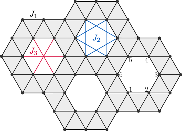
Figure 1: Maple-leaf lattice with nearest-neighbor coupling $J_{1}$ and further-neighbor cross-plaquette couplings $J_{2}$ and $J_{3}$. The unit cell consists of the six sites that make up a hexagonal plaquette.

The exemplary textbook example of frustration is a triangular motif with antiferromagnetically interacting spins at its vertices [33]. Their edge-shared tessellation forms a triangular lattice which has been fertile ground for skyrmion physics [29, 34, 35, 36, 20, 37]. For an $S=1/2$ Heisenberg model with first $J_{1}$, second $J_{2}$ and third $J_{3}$ neighbor antiferromagnetic couplings on the triangular lattice there was an early proposal for a chiral spin liquid [38], which has lately been challenged [39], and its existence remains debatable. Additional scalar spin chiral interactions need to be invoked to realize a stable chiral spin liquid phase which emerges out of quantum melting of noncoplanar tetrahedral order in the corresponding classical model [40, 41, 7]. On the other hand, a corner-sharing tessellation of triangles, which leads to only a marginal alleviation of frustration, forms the kagome lattice —alternatively viewed as a $1/4$ site-depletion of the triangular lattice. Here, for antiferromagnetic $J_{1}$ and $J_{2}$, the inclusion of antiferromagnetic $J_{3}$ interactions across hexagons alone suffices to trigger a robust chiral spin liquid of the Kalmeyer-Laughlin type, possibly descending from quantum melting of parent cuboc orders [42, 43, 44, 45, 46], while for ferromagnetic $J_{1}$, a similar scenario has been argued for in Refs. [47, 10, 48]. An analogous situation could potentially be realized on the square-kagome lattice where a multitude of noncoplanar orders, including novel cuboc states, have recently been reported in the classical Heisenberg model with competing long-range cross-plaquette interactions [32]. Very recently, geometrical frustration inherent to various fullerene molecules has been shown to induce noncoplanar textures and chiral spin states in Heisenberg models [49].

In this work, we consider a comparatively sparse $1/7$ site-depletion of the triangular lattice that leads to the five-fold coordinated maple-leaf lattice [50, 51, 52, 53, 54, 55, 56, 57, 58, 59, 60, 61] — a uniform tiling of triangles and hexagons, as shown in Fig. 1 below. Hence, both in terms of the depletion density and coordination number, the maple-leaf lattice is intermediate between the triangular and kagome lattices, and one may wonder about the potential existence of a robust chiral spin liquid. As a guiding light in search of this phase on the maple-leaf lattice, it is important to first identify regions in parameter space of classical Heisenberg models which are host to noncoplanar magnetic orders. To this end, we consider a spatially isotropic Heisenberg model with antiferromagnetic $J_{1}$ and $J_{2}$ interactions, and, motivated by the kagome, include $J_{3}$ interactions across hexagonal plaquettes. Our study reveals a rich landscape comprised of four noncoplanar classical orders, together with two coplanar orders. In particular, this includes a previously unreported novel configuration where the spins point to the vertices of an icosahedron, which we dub icosahedral order, inspired by the cuboctohedral orders reported on the kagome lattice [4]. Employing a state-of-the-art implementation of the pseudo-fermion functional renormalization group approach [62], we assess the impact of quantum fluctuations for $S=1/2$ and find an extended region in the $J_{2}$-$J_{3}$ plane which lacks long-range magnetic order. Importantly, the span of this nonmagnetic region encompasses regions classically occupied by noncoplanar orders, and could thus tentatively be associated with a putative chiral spin liquid. Furthermore, since the maple-leaf lattice lacks reflection symmetry about any straight line, the putative chiral spin liquid could lie outside the realm of the standard Kalmeyer-Laughlin paradigm which involves breaking of reflection symmetry up to time-reversal.

This paper is structured as follows. We first introduce the model in Section II. The classical phase diagram is discussed in Section III, before we turn to the effects of quantum fluctuations in Section IV.

II Model

The maple-leaf lattice [50] is an Archimedean lattice that is obtained by a periodic depletion of 1/7 of the sites of the triangular lattice, as visualized in Fig. 1. Its coordination number is $z=5$ and, therefore, it is intermediately frustrated between the kagome $(z=4)$ lattice and the triangular $(z=6)$ lattice. It can be described by the lattice vectors

$$\mathbf{a}_{1} =\left(\frac{3\sqrt{3}}{2},-\frac{1}{2}\right), \mathbf{a}_{2} =\left(\sqrt{3},2\right),$$

and a unit cell comprising six sites with relative coordinates

$$\mathbf{\delta}_{1} =\left(0,0\right), \mathbf{\delta}_{2} =\left(\frac{\sqrt{3}}{2},-\frac{1}{2}\right),$$

$$\mathbf{\delta}_{3} =\left(\sqrt{3},0\right), \mathbf{\delta}_{4} =\left(\sqrt{3},1\right),$$

$$\mathbf{\delta}_{5} =\left(\frac{\sqrt{3}}{2},\frac{3}{2}\right), \mathbf{\delta}_{6} =\left(0,1\right).$$

With the three different couplings $J_{1}$ (nearest-neighbor), as well as $J_{2}$ and $J_{3}$ (cross-plaquette), as indicated in Fig. 1, the Heisenberg Hamiltonian on the maple-leaf lattice can be written as

$$\mathcal{H}=\sum_{\langle{i,j}\rangle\in a}J_{a}\,\mathbf{S}_{i}\cdot\mathbf{S}_{j}\,,$$ (1)

where $a=\{1,2,3\}$ runs over the three different types of bonds.

III Classical Phase Diagram

To study the classical ground-state phase diagram of the Heisenberg model on the maple-leaf lattice, Eq. (1), we employ large-scale classical Monte Carlo simulations, which we combine with a semi-analytical method that allows us to determine the exact phase boundaries (for details see Appendix A).

Upon varying the cross-plaquette interactions $J_{2}$ and $J_{3}$ (where $J_{1}=1$ is fixed to be antiferromagnetic), we indeed find a number of different ground-state phases, including coplanar and noncoplanar magnetic orders, as summarized in the classical phase diagram of Fig. 2. From the representative common origin plots of the ground-state real-space spin configurations (and also the static spin structure factors) next to the phase diagram, one can see at first glance that the six phases found (labeled I to VI) are clearly distinct from one another.

The coplanar phases I and III appear in the form of two different six-sublattice ordered states, the first of which has already been described in the context of the quantum model on the maple-leaf lattice without cross-plaquette interactions. The remaining four phases come in different noncoplanar orders, including commensurate variants (phases II and VI) as well as incommensurate ones (phases IV and V). We will provide details about each phase in the remainder of this section. It is noteworthy that the ground states of all phases, with the exception of phases IV and V, can also be calculated analytically using the Luttinger-Tisza (LT) approach, see Appendix C. For phases IV and V, however, the LT approach yields unphysical ground states with a spin dimension greater than 3.

Figure 2: Classical phase diagram of the maple-leaf lattice with six different phases (labeled I-VI) as a function of $J_{2}$ and $J_{3}$ (and fixed nearest-neighbor coupling $J_{1}=1$). Besides indicating the phase boundaries (solid lines), the phases are described by symmetry (with $D_{n}$ referring to the dihedral group of order $n$ and $T$ to tetrahedral symmetry), and coplanarity. Also, we show common origin plots and spin structure factors from Monte Carlo simulations ($T/J_{1}=10^{-4},\ N=864$) for each phase to the right of the phase diagram.

III.1 Coplanar Orders

We start with the coplanar ground states of phase I and phase III, which make up large parts of the lower half and the upper right corner of the classical phase diagram of Fig. 2 respectively.

III.1.1 Coplanar phase I with $D_{3}$ symmetry

This order has already been described as the ground state in the classical limit of the quantum maple-leaf Heisenberg model in Refs. [52, 53, 54, 58] in the special case $J_{2}=J_{3}=0$ and is in full agreement with our numerical and analytical results. It consists of six sublattices of spins and a three times larger magnetic unit cell, as indicated in Fig. 3(a). Within one geometrical unit cell, neighboring spins form an angle

$$\alpha=\arctan\left(\frac{\sqrt{3}}{3+2J_{3}}\right)+\pi$$ (2)

while next-nearest neighbors are parallel. Equivalent spins in two neighboring geometric unit cells are rotated by $2\pi/3$. Its energy can be given explicitly as

$$E_{\text{I}}=-\frac{1}{2}\left(1-2J_{2}+\sqrt{3+3J_{3}+J_{3}^{2}}\right)\,.$$ (3)

The symmetry of this ground state is given by the dihedral group of order 3, $D_{3}$. For the special case $J_{3}=-2$, the six different spin vectors form a regular hexagon with $D_{6}$ symmetry. In the case $J_{3}=-1$, on the other hand, the ground state becomes a $120^{\circ}$ state which still has $D_{3}$ symmetry.

III.1.2 Coplanar phase III with $D_{6}$ symmetry

The rigid coplanar order of phase III, found in the upper right corner of the phase diagram, also has six sublattices of spins, but the magnetic unit cell coincides with the geometrical unit cell. Within each unit cell, each spin points to a different corner of a regular hexagon (see Fig. 3(b)) and nearest neighbors (within a unit cell) form an angle of $\pi/3$. The corresponding ground-state energy is

$$E_{\text{III}}=-\frac{1}{2}\left(1+J_{2}+J_{3}\right)\,.$$ (4)

and the symmetry group of the ground state is the dihedral group of order 6, $D_{6}$.

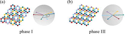
Figure 3: Coplanar orders. (a) The ground state of phase I has six sublattices of spins and a 18-site magnetic unit cell (outlined in red). Within one geometrical unit cell, neighboring spins form an angle $\alpha$ (for example, yellow and green spins) while next-nearest neighbors are parallel. Equivalent spins in two neighboring geometric unit cells are rotated by $2\pi/3$ (for example, yellow and light blue spins). (b) In phase III, the ground state has six sublattices as well, but the magnetic unit cell coincides with the geometrical unit cell. Within each unit cell, each spin points to a different corner of a regular hexagon and nearest neighbors (within a unit cell) form an angle of $\pi/3$.

III.2 Noncoplanar Orders

We now come to a discussion of the various noncoplanar magnetic orders, starting with the two commensurate structures found in phases II and VI of the phase diagram. The starting point for all semi-analytical descriptions are numerical Monte Carlo ground states at $T=10^{-4}$ with fixed $J_{1}=1$.

III.2.1 Noncoplanar phase II with $T\times\mathbb{Z}_{2}$ symmetry

The ground state of phase II consists of 24 sublattices of spins and the magnetic unit cell spans the same amount of sites, as shown exemplarily in Fig. 4(a) for $J_{2}=1.0$ and $J_{3}=0.5$. A symmetry analysis of the ground state reveals that it is described by the symmetry group $T\times\mathbb{Z}_{2}$, the direct product of the tetrahedral group without reflections $T$ and the group $\{\text{id},-\text{id}\}\cong\mathbb{Z}_{2}$. The energy of this state can be expressed as a function of two parameters $\lambda$ and $\alpha$ as

$$E_{\text{II}}=\frac{1}{6}\Big{[} -7+12\lambda^{2}-9J_{2}\lambda^{2}+6J_{2}-3J_{3}$$

$$+2\lambda\sqrt{6-6\lambda^{2}}\cos\alpha+4\lambda^{2}\cos 2\alpha$$

$$+2\lambda\sqrt{2-\lambda^{2}}\sin\alpha+2\sqrt{3}\lambda^{2}\sin 2\alpha\Big{]}\,.$$ (5)

Minimizing this expression for $J_{2}=1.0$ and $J_{3}=0.5$ yields $E_{\text{II},\text{semi-analytical}}=-1.41782$ which fits well with the Monte Carlo result for the same parameters $E_{\text{II},\text{MC}}=-1.417(5)$.

III.2.2 Noncoplanar phase VI with $T$ symmetry

The magnetic order of phase VI also has a 24-site magnetic unit cell, but only 12 sublattices of spins. In general, these point to the corners of a deformed icosahedron, which becomes regular in the special case $J_{2}=0.0,J_{3}=-1.0$ shown in Fig. 4(b). Its symmetry is described by the tetrahedral symmetry group without reflections $T$ (for the aforementioned special case it becomes the icosahedral symmetry group $I_{h}$). The general expression for the ground-state energy as a function of two parameters $\lambda$ and $\alpha$ is

$$E_{\text{VI}}=\frac{1}{6}\Big{[} 3+6J_{2}-9J_{2}\lambda^{2}+3J_{3}+4\lambda\sqrt{6-6\lambda^{2}}\cos\alpha$$

$$+3\lambda^{2}\cos 2\alpha-\sqrt{3}\lambda^{2}\sin 2\alpha-6\lambda^{2}\Big{]}\,.$$ (6)

Minimizing this term for, e.g., $J_{2}=0.5$ and $J_{3}=-0.5$, leads to $E_{\text{VI},\text{semi-analytical}}=-1.60183$ in line with the corresponding Monte Carlo result $E_{\text{VI},\text{MC}}=-1.601(4)$.

In the following, we conclude this report on the various noncoplanar orders on the maple-leaf lattice with the two incommensurate spiral structures of phases IV and V.

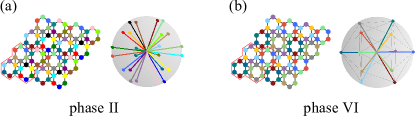
Figure 4: Noncoplanar orders II and VI. (a) The ground state of phase II has 24 sublattices of spins and a magnetic unit cell with as many sites (outlined in red in the realspace arrangement on the left). Right: common origin plot of the 24 spin directions. (b) The ground state of phase VI has a 24-site magnetic unit cell as well, but only 12 sublattices of spins. In general, these point to the corners of a deformed icosahedron which becomes regular in the special case $J_{2}=0.0,J_{3}=-1.0$ (shown here).

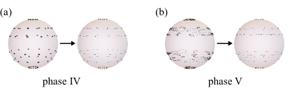
Figure 5: Noncoplanar spiral orders IV and V. (a) Left: common origin plot of the Monte Carlo ground state of spiral phase IV (for $J_{2}=1.0$ and $J_{3}=0.7$) with $N=864$ spins. Right: These can be grouped into $M=72$ unique directions and described analytically (see text). The resulting order has $D_{12}$ symmetry. (b) The same applies in the case of the spiral ground state of phase V, here shown for $J_{2}=1.0$ and $J_{3}=0.6$.

III.2.3 Noncoplanar phase IV with $D_{12}$ symmetry

In the spiral phase IV, as depicted in the common origin plot on the left of Fig. 5(a) for $J_{2}=1.0$ and $J_{3}=0.7$, we are left with $M=72$ unique spin vectors after grouping those spins that point into the same direction (cf. the corresponding plot on the right of the very same figure). This state is symmetric under actions of the dihedral group of order 12, $D_{12}$, as well as under mirroring $z\mapsto-z$. The ground-state energy $E_{\text{IV}}$ can explicitly be expressed analytically as a function of eight parameters (which is too long to be specified here). Its minimization yields $E_{\text{IV},\text{semi-analytical}}=-1.35069$, consistent with the Monte Carlo result $E_{\text{IV},\text{MC}}=-1.350(5)$.

III.2.4 Noncoplanar phase V with $D_{12}$ symmetry

For the spiral phase V, we consider the numerical Monte Carlo ground state for $J_{2}=1.0$ and $J_{3}=0.6$, as shown in the common origin plot on the left of Fig. 5(b). After grouping the $N=864$ spin vectors according to their unique directions, we are left with $M=72$ unique spin vectors, which can be divided into six groups with constant $z$-component, as visualized on the right of Fig. 5(b). Taking into account $D_{12}$ symmetry and invariance under $z\mapsto-z$, the state can be described by three $z$-components $z_{1}$, $z_{2}$, and $z_{3}$, and the difference angle $\delta\phi$ between the azimuth angles of the spins on the two lower circles on the one hand, and the upper circle on the other. With these parameters, the ground-state energy takes the form

$$E_{\text{V}}=\frac{1}{12}\Bigg{[} -1-4z_{1}^{2}-z_{2}^{2}-2\sqrt{3-3z_{2}^{2}}\sqrt{1-z_{3}^{2}}$$

$$-J_{3}\left(1+z_{1}^{2}+2z_{2}^{2}+2z_{3}^{2}\right)$$

$$-4J_{2}\Big{(}-z_{2}z_{3}+z_{1}(z_{2}z_{3})$$

$$+\sqrt{1-z_{2}^{2}}\sqrt{1-z_{3}^{2}}\Big{)}+\sqrt{1-z_{1}^{2}}\Bigg{(}\Big{(}2\sqrt{1-z_{2}^{2}}$$

$$-(2+\sqrt{3})J_{2}\big{(}\sqrt{1-z_{2}^{2}}-\sqrt{1-z_{3}^{2}}\big{)}\Big{)}\cos\delta\phi$$

$$+\Big{(}(-4+2\sqrt{3})\sqrt{1-z_{2}^{2}}$$

$$+J_{2}\big{(}\sqrt{1-z_{2}^{2}}-\sqrt{1-z_{3}^{2}}\big{)}\Big{)}\sin\delta\phi\Bigg{)}\Bigg{]}\,.$$ (7)

Minimization of this energy yields $E_{\text{V},\text{semi-analytical}}=-1.32311$ in good agreement with and slightly smaller than the Monte Carlo result $E_{\text{V},\text{MC}}=-1.322(7)$ for the same parameters.

A compact summary that characterizes all six phases of the phase diagram of Fig. 2 by the ground-state symmetry, and corresponding q vectors, if any, is given in Table 1.

Phase	Symmetry	$\mathbf{q}$ vectors	Semi-analytical
			$N$	$M$	$K$	# parms
I	$D_{3}$	$\left(\frac{2\pi}{3},-\frac{2\pi}{3}\right)$	–	–	–	–
II	$T\times\mathbb{Z}_{2}$	$(0,\pi),(\pi,0),(\pi,\pi)$	–	–	–	–
III	$D_{6}$	(0,0)	–	–	–	–
IV	$D_{12}$	–	864	72	6	6
V	$D_{12}$	–	864	72	3	4
VI	$T$	$(0,\pi),(\pi,0),(\pi,\pi)$	–	–	–	–

Table 1: Symmetry characterization of the six ground-state phases of the phase diagram Fig. 2. Given are the ground-state symmetry (second column), and the $\mathbf{q}$ vectors of each phase (if any, third column). For the two semi-analytically described phases (IV and V), the compression of the parametrization of the spin spirals via clustering and symmetrization is given in the four columns on the right. Technically, the semi-analytical description is obtained by starting with a common origin plot with $N=864$ spins sampled at $T=10^{-4}$ for a linear system size $L=12$, and is then given in terms of $M$, $K$, and the number of needed parameters (last column) to describe the phase (see Appendix A for details).

IV Quantum Phase Diagram

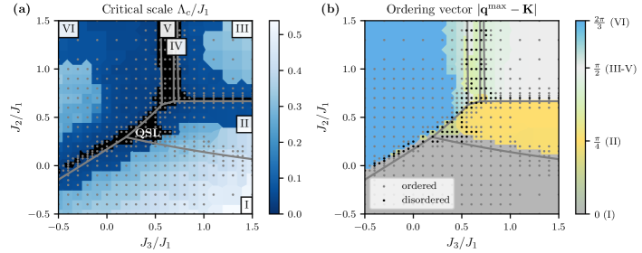
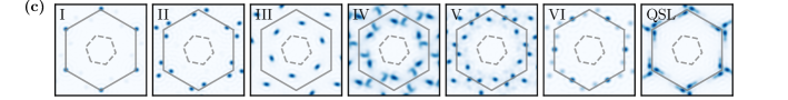
Figure 6: Quantum phase diagram as obtained from the pf-FRG. (a) Critical scale $\Lambda_{c}$ where the renormalization group flow exhibits an instability, signaling the formation of long-range order. In the black regions the flow shows no instablility ($\Lambda_{c}=0$), indicating a disordered ground state. The gray dots indicate the couplings for which calculations were performed. (b) Distance of the momentum where the structure factor is maximal $\mathbf{q}^{\mathrm{max}}$ to the $\mathbf{K}$-point of the extended Brillouin zone. Quantum disordered points that show no flow breakdown $(\Lambda_{c}=0)$ are colored black. The gray lines are the classical phase boundaries. (c) Structure factors at the same parameters as shown for the classical case in Fig. 2. The dashed and solid gray lines show the first and extended Brillouin zones, respectively.

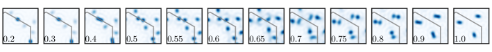
Figure 7: Quantum structure factor evolving from phase III to VI for fixed $J_{2}/J_{1}=1$ and varying $J_{3}/J_{1}$ (indicated in the bottom left corners). We observe a seemingly continuous evolution with no clearly distinct signatures of phases V and VI.

In the previous section we unveiled the existence of a plethora of classically ordered phases in the maple-leaf model defined in Fig. 1. Most notably, we identified four phases (II, IV, V and VI) with a noncoplanar ground state. Now, we turn to the question of how these phases are affected by quantum fluctuations. Particular interest lies in finding parameter regimes where fluctuations melt the classical noncoplanar order into a ground state with restored spin rotational symmetry. Such a state would then be a strong candidate for a chiral quantum spin liquid [10, 6, 7]. To achieve this, we replace the classical spins in the original model by $S=1/2$ spin operators. We then calculate the ground-state phase diagram of the resulting quantum model using the pseudo-fermion functional renormalization group (pf-FRG), a by now well-established method for distinguishing between magnetically ordered and disordered regimes at zero temperature [62].

To probe for magnetic order in the ground state of a given spin Hamiltonian, we use the pf-FRG to calculate the flow of the (static) spin-spin correlation defined as

$$\chi_{ij}^{\Lambda}=\int_{0}^{\infty}\!\!\!d\tau e^{i\omega\tau}\!\left\langle\hat{T}_{\tau}\hat{S}^{z}_{i}(\tau)\hat{S}^{z}_{j}(0)\right\rangle\Big{|}^{\Lambda}_{\omega=0}$$ (8)

where $\hat{T}_{\tau}$ is the time-ordering operator in imaginary time $\tau$ and $\Lambda$ is an infrared cutoff, or RG scale, artificially introduced into the theory. A Fourier transformation then leads to the flow of the magnetic structure factor. If the ground state of the Hamiltonian under consideration exhibits magnetic order, this flow will exhibit a divergence, or flow breakdown, at a finite critical scale $\Lambda_{c}$ for the Bragg momenta characterizing the incipient order. Conversely, in the absence of a flow breakdown, the ground state is anticipated to be a disordered state, indicative of a potential quantum spin liquid. More details on the pf-FRG and the criteria used to distinguish ordered from disordered states are provided in Appendix B.

In practice, we calculate the flow using the PFFRGSolver.jl Julia package, featuring state-of-the-art, adaptive integration schemes [63] for solving the pf-FRG flow equations. To discretize the continuous Matsubara frequency dependence of the four-point correlators, we choose an adaptive grid of $n_{\Omega}=40$ bosonic and $n_{\nu}=35\times 35$ fermionic Matsubara frequencies. We use lattice truncations of up to $L=15$, i.e., correlations are set to zero beyond a bond distance of 15. Using this setup, we calculate the quantum analog to the classical phase diagram in Fig. 2, with a focus on identifying quantum disordered parameter regimes. The result for the critical scale is shown in Fig. 6(a), while Fig. 6(b) shows the ordering vectors (i.e. the momenta where the structure factor is maximal) and Fig.6(c) illustrates instances of the complete structure factor within the various phases we have identified.

IV.1 Quantum structure factors

Before discussing the possibility of quantum disordered phases, let us first compare the indication of order visible in the pf-FRG structure factors with our classical analysis. Not surprisingly, the ground-state structure factors agree well with the classical case deep in the phases I, II, III and VI [compare Fig. 2 with Fig. 6(c)]. Nonetheless, in the proximity to certain phase boundaries, notable deviations emerge.

Most prominently, within the region between phases III and VI, we don’t observe two distinct phases IV and V, as identified in the classical model. Instead, as depicted in Fig. 7, the structure factor continuously evolves from phase III to phase VI, showing peaks at incommensurate momenta in between. A similar situation arises in proximity to the triple point where phases I, II and VI converge. Here, the pf-FRG again reveals an extended region with a structure factor maximum at an incommensurate momentum.

Incommensurate spin configurations can not be faithfully captured with periodic boundary conditions on a finite lattice, as utilized by our Monte Carlo calculations. This limitation is likely why, in the classical analysis, we identified only distinct phases with finite magnetic unit cells. In contrast, the pf-FRG employs open boundary conditions and thus avoids this issue. We note that, in both incommensurate regimes, the ordering vectors from pf-FRG align remarkably well with the momenta $\mathbf{q}^{\mathrm{min}}$ that minimize the energy in an unconstrained Luttinger-Tisza (LT) approach [64, 65]. In this LT approach, the constraint of constant spin length is softened enabling a straight-forward diagonalization of the Hamiltonian in momentum space (see Appendix C for details). It has been argued that this approach provides an improved approximation to the quantum problem compared to a purely classical analysis [66]. More importantly, it takes into account the full infinite lattice, allowing for the description of both commensurate and incommensurate ground-state orders.

IV.2 Disordered phases

Returning to the discussion of disordered, putative quantum spin liquid phases, they exactly seem to appear in the parameter regions where the classical and quantum structure factors disagree. In the pf-FRG, these phases manifest themselves by the absence of a flow breakdown ($\Lambda_{c}=0$), illustrated by the black colored regions in Fig. 6(a). Most prominently, we observe an extended quantum disordered regime close to the triple point where the phases I, II and VI converge, which extends further into the classical noncoplanar phase II with $T\times\mathbb{Z}_{2}$ symmetry. Here, the interplay of quantum fluctuations and the competition of three neighboring phases seems to suppress the magnetic order, making the regime a promising candidate for an extended chiral quantum spin liquid phase.

Furthermore, the incommensurate regime between phases III and VI also exhibits a vanishing critical scale. However, in this case the continuous evolution of the structure factor, and the resulting proximity to a spectrum of many different orders at any given point along the evolution, may pose a challenge for the pf-FRG to correctly identify a flow breakdown at a specific ordering vector. Incommensurate states also tend to have a flow breakdown at lower critical scales, further complicating the numerical identification. We can, therefore, not clearly determine whether this region is genuinely quantum disordered or if it is an artifact of our calculation.

V Conclusions and outlook

We explore the classical and quantum phase diagram of the spatially isotropic Heisenberg antiferromagnet on the maple-leaf lattice in the presence of long-range interactions. In search of noncoplanar magnetic orders, we show that the minimal set of couplings that need to be invoked to stabilize these orders are cross-hexagonal third neighbor antiferromagnetic interactions on top of the nearest-neighbor antiferromagnetic Heisenberg model –similar to the kagome lattice where such couplings are known to trigger cuboc orders. A comprehensive classical Monte Carlo study finds a rich variety of noncoplanar states, including a new type of order wherein the spins point to the vertices of an icosahedron (dubbed icosahedral order), as well as complex incommensurate noncoplanar spirals. These states feature large magnetic unit cells with a highly intricate structure, but with the salient feature that they lend themselves to a semianalytical construction. We provide an optimal parameterization of the spin configuration of these states based on a careful symmetry analysis. This allows for obtaining explicit expressions (depending on only a few parameters) for their ground-state energy as a function of the interactions, which in turn permits us to accurately establish the phase boundaries between these complex phases. It is highly plausible that considering a more generalized symmetry-allowed model with all three couplings at first, second, and third neighbors being different with possible ferro- and antiferromagnetic combinations, would give us access to a comparatively richer landscape of exotic noncoplanar orders.

In addition to the ground state, we study the thermodynamics of noncoplanar states using classical Monte Carlo simulations. The behavior of the specific heat points to a finite-temperature phase transition in this classical two-dimensional model, as expected due to the chiral nature of the noncoplanar ground states [4]. In the limit of low spin values, e.g., $S=1/2$, one may expect that strong quantum fluctuations preclude the formation of long-range magnetic order while the long-range order in chirality survives, thus possibly stabilizing a chiral spin liquid. Given that the maple-leaf lattice lacks reflection symmetry about any straight line, the issue concerning which lattice symmetries could be broken up to time-reversal (i.e., allowed chiral classes) in order to respect “$PT$” theorem (for $U(1)$ QSLs) is worth examining. Identifying the allowed symmetry patterns and microscopic nature of this putative QSL phase would involve a systematic projective symmetry group classification of chiral mean-field Ansätze with $U(1)$ and $\mathbb{Z}_{2}$ low-energy gauge groups [10]. The ground-state energies and correlation functions of the corresponding Gutzwiller projected states could then be obtained within a variational Monte Carlo scheme [67, 68], and compared to the structure factors obtained from pf-FRG in the current work. Alternatively, these Ansätze could be analyzed within a pf-FRG framework itself by performing a self-consistent Fock-like renormalized mean-field scheme to compute low-energy theories for emergent spinon excitations but using effective vertex functions instead of the bare couplings [69]. Indeed, (gapless) $U(1)$ chiral spin liquids displaying cuboc type magnetic correlation profiles have been reported to be energetically competitive variational ground states in the $S=1/2$ $J_{1}$-$J_{2}$-$J_{d}$ Heisenberg model [10, 47]. In a similar vein, it would be interesting to identify the QSL whose structure factor profile resembles that of the novel icosahedral order, and obtain a knowledge of its low-energy gauge structure, $U(1)$ or $\mathbb{Z}_{2}$, gapped vs gapless, etc. It would also be worthwhile to study the propensity towards dimerized states [70, 71, 72, 73], since such $J_{3}$ couplings on the kagome lattice are known to induce valence bond crystals in the vicinity of chiral spin liquids [43].

From a materials perspective, a number of experimentally studied natural minerals [74, 75, 76, 77] and synthetic crystals [78, 79, 80, 81] have come into the limelight. Subsequent theoretical analysis of the complex frustration mechanism at play in these compounds is in a nascent stage, both as regards the nature of magnetic interactions and the consequences of their interplay [82, 83]. It can be envisaged that, either in synthesis of polymorphs, or in naturally occuring minerals, a scenario similar to that in the kagome materials kapellasite [84] and haydeite [85] plays out, whereby the nonmagnetic ions (in these cases Zn and Mg, respectively), occupy the centers of the hexagons, thus spanning the pairs of magnetic ions connected by $J_{3}$. The synthesis of compounds with such superexchange paths is likely to trigger a sizeable $J_{3}$ interaction, and depending on its strength could induce magnetic fluctuations displaying profiles of noncoplanar orders, as have been observed in kapellasite which displays cuboc-2 type magnetic fluctuations [86].

Data availability.–

The numerical data shown in the figures is available on Zenodo [87].

Appendix A Supplementary material on the classical Monte Carlo simulations

For the analysis of the classical phase diagram and the different ground states, we use a combination of classical Monte Carlo simulations in conjunction with a semi-analytical method, which we briefly explain in this appendix.

A.1 Monte Carlo simulations

All Monte Carlo simulations are performed on finite lattices of $L\times L$ unit cells with periodic boundary conditions, that is, $N=6L^{2}$ spins ($L=12$ unless stated otherwise). Local updates are performed with the Metropolis-Hastings algorithm. To resolve the thermal selection of ground states by thermal order-by-disorder effects at very low temperatures, we employ a parallel tempering/replica exchange Monte Carlo scheme [88, 89] with 192 logarithmically spaced temperature points between $T_{\text{min}}=10^{-4}$ and $T_{\text{max}}=10$. These replicas are simulated simultaneously such that after every sweep, spin configurations of neighboring replicas are attempted to be exchanged according to some probability. As a result, the individual replicas perform a random walk in temperature space and can thus easily escape from local minima at low temperatures. We have taken care to check the thermalization of our parallel tempering scheme against feedback-optimized temperatures. [90]. For the specific heat data, a conventional Monte Carlo scheme without parallel tempering and 192 linearly spaced temperature points between $T_{\text{min}}=0.02$ and $T_{\text{max}}=0.5$ is employed. In all cases, measurements are performed over $5\cdot 10^{8}$ sweeps after a thermalization period of $10^{8}$ sweeps. The static spin structure factors shown in the classical phase diagram (Fig. 2) are obtained from the Fourier transform of the Monte Carlo equal-time real space spin-spin correlations, that is,

$$S(\mathbf{q})=\frac{1}{N}\sum_{i,j=1}^{N}\langle\mathbf{S}_{i}\cdot\mathbf{S}_{j}\rangle e^{i\mathbf{q}\cdot(\mathbf{r}_{i}-\mathbf{r}_{j})}\,,$$ (9)

where $\mathbf{q}$ is a momentum inside the extended Brillouin zone, and $\mathbf{r}_{i}$ denotes the position of site $i$.

Figure 8: Ground-state energies from Monte Carlo simulations at low temperatures $(T=10^{-4})$ for (a) fixed $J_{3}=0.0,1.0$, and (b) fixed $J_{2}=0.0,1.0$, respectively. The insets show the corresponding second derivatives, $E^{\prime\prime}/N$. These show clearly visible features exactly at the semi-analytically determined phase boundaries (indicated as vertical dashed lines).

A.2 Semi-analytical method

We also use a semi-analytical approach presented in [32], which works as follows: Starting from a ground state for a system of $N$ classical spins $\mathbf{S}_{i}$, which we obtain numerically from a Monte Carlo simulation, we first transform onto the eigenbasis of the corresponding tensor of inertia. Then we form groups of spin vectors that point approximately in the same direction, i.e. that fulfill, e. g., $\mathbf{S}_{i}\cdot\mathbf{S}_{j}\geq 0.995$. This results in a set of $M$ different spin directions, which is further reduced by guessing their symmetry group. In the end, we have $K$ different spin directions for the ground state, from which we obtain all others by applying symmetry operations. Next, we calculate the energy of the spin configuration ${\mathcal{H}}(\alpha_{1},\ldots,\alpha_{n})$ as a function of some parameters $\alpha_{1},\ldots,\alpha_{n}$ that describe the position of the remaining $K$ spin vectors. These parameters have different meanings for the different phases, e. g., they could be some $z-$ values that are constant for groups of spin vectors or certain difference angles between configurations of groups of spins. We need at most $n=2K-1$ parameters to characterize the spin configuration, but often less, see Table 1. The energy ${\mathcal{H}}(\alpha_{1},\ldots,\alpha_{n})$ is then numerically minimized starting with the initial numerical values of the parameters corresponding to the $K$ spin vectors. It should have become clear that the semi-analytical method cannot be applied schematically, but requires a certain amount of intuition. Incorrect identifications of closely neighboring spins are usually reflected in ground-state energies that are too high. Conversely, a slight lowering of the numerical initial energy is an indication of a successful application of the method.

A.3 Supplemental numerical data

Let us supplement the results for the classical phase diagram discussed in the main text with additional data sets for (i) cuts of the ground-state energy and (ii) for the thermodynamic signatures of the classical phases in specific heat traces.

A.3.1 Ground-state energy

Cuts of the Monte Carlo ground-state energy as a function of $J_{2}$ and $J_{3}$ are presented in Fig. 8. These underline the good interplay of Monte Carlo numerics on the one side, and semi-analytical method on the other side: The insets in Fig. 8 display the second derivatives of the Monte Carlo ground-state energy where the peaks indicate phase transitions along with the semi-analytically determined phase boundaries. Note that it is precisely at these boundaries that the Monte Carlo energies have clearly visible features, which is a confirmation of the accuracy of the (semi-analytically) determined phase boundaries.

A.3.2 Specific heat

Specific heat traces for the six phases are shown in Fig. 9. The spiral phases IV and V show complicated behavior; due to their incommensurability, these phases depend very sensitively on finite-size effects. In contrast, the four phases I, II, III, and VI, display single peaks at some finite temperature that scale with the system size—a scaling behavior that is expected for a thermal ordering phase transition.

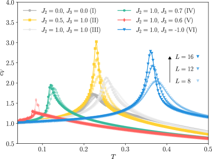
Figure 9: Specific heat traces from Monte Carlo simulations for all six phases, color-coded the same way as in the phase diagram Fig. 2. The spiral phases IV and V (green and red, respectively) show complicated behavior indicating a sensitive dependence on finite-size effects. The four commensurate phases I (dark gray), II (yellow), III (light gray), and VI (blue), display a scaling behavior that is expected for a thermal phase transition with a single peak that grows with system size. Note, that for phase I, the simulated system sizes are $L=9,12,15$ to ensure commensurability of the underlying order with the lattice.

Appendix B Supplementary material on the Pseudo-Fermion Functional Renormalization Group

To calculate the quantum phase diagram in Fig. 6 we employ pseudo-fermion functional renormalization group (pf-FRG) calculations. In this appendix, we shortly state the idea of the pf-FRG approach, and give references for readers interested in more details. We then describe our precise criterion for distinguishing disordered from ordered ground states used in analyzing the pf-FRG flow. Finally, we provide additional cuts through the quantum phase diagram for a better illustration of the transitions between the observed phases.

B.1 Method

The core concept of the pf-FRG involves avoiding the simultaneous treatment of all energy scales in the quantum problem at once. Instead, the approach starts at a known high-energy limit and subsequently incorporates lower energy scales in an iterative manner. To this end, an infrared cutoff, or RG Scale, $\Lambda$ is inserted into the model, so that in the high-energy limit $(\Lambda\to\infty)$ all correlation functions are completely determined by the bare couplings in the Hamiltonian, and in the low-energy limit $(\Lambda=0)$ the full theory is recovered. In our case, the cutoff is implemented in Matsubara frequency space by multiplying the bare propagator with a continuous regulator function. The interpolation between high and low energies is governed by an infinite hierarchy of differential equations, called flow equations. Employing the Katanin truncation [91], we approximate this infinite hierarchy by a finite number of flow equations for the two- and four-point correlations, which we can—under certain approximations—solve numerically using the the PFFRGSolver.jl Julia package [63]. From the flow of these correlations we can then determine if the ground state of a given spin model is likely ordered or disordered. Details on this are given in the appendix below. For readers interested in more details on the pf-FRG approach we refer to the review [62], and for more details on our specific implementation, we refer to [92].

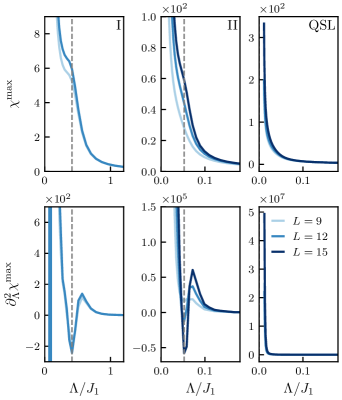
Figure 10: Renormalization group flow of the structure factor in ordered (I and II) and disordered (QSL) phases. The top row shows the structure factor flow at the momentum where it is maximal. The bottom row shows the second derivative of the flow with respect to the cutoff $\Lambda$, in which non-monotonic features signal the development of a flow breakdown. The position of the flow breakdown, the critical scale $\Lambda_{c}$, is depicted by the dashed gray lines. In the quantum disordered regime (right column), no flow breakdown occurs.

B.2 Flow breakdown criterion

To probe for magnetic order in the ground state of a given spin Hamiltonian, we calculate the (static) spin-spin correlation $\chi_{ij}^{\Lambda}$ defined in Eq. (8) from the two- and four-point correlations. We then Fourier transform $\chi_{ij}^{\Lambda}$ to obtain the flow of the (static) structure factor. If the ground state of the Hamiltonian under consideration exhibits magnetic order, this flow will show a divergence, or flow breakdown, at a finite critical scale $\Lambda_{c}$ for the Bragg momenta characterizing the incipient order. If, on the other hand, there is no flow breakdown, the ground state is expected to be a disordered, putative quantum spin liquid state. In practice, the lattice truncation $L$ and the truncation of the flow equations will usually soften the divergence indicating a flow breakdown to a cusp or a peak, which becomes more prominent with increasing $L$. The flow of a disordered state, on the other hand, is expected to stay smooth and convex down to the lowest considered RG scale (in our case $\Lambda_{\mathrm{min}}=0.01|J|$, with $|J|^{2}=J_{1}^{2}+J_{2}^{2}+J_{3}^{2}$ as normalization). We, therefore, identify any non-monotonicity in the second derivative of the structure factor flow as a flow breakdown, under the condition that it becomes more pronounced with increasing lattice size. For this comparison, we use up to three different truncation lengths $L=9,12,15$. Examples of structure factor flows and their second derivative are shown in Fig 10. In the ordered regime, the second derivative shows a clear non-monotonicity, resulting in a cusp in the structure factor flow, and a clear lattice size dependence. In the disordered case, both the flow and its second derivative are smooth, monotonous, and essentially lattice size independent, signaling the absence of long-range order.

B.3 Cuts through the quantum phase diagram

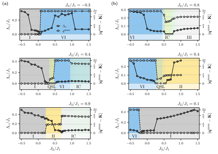
Figure 11: Cuts through the quantum phase diagram shown in Fig. 6. Gray circles depict the critical scale $\Lambda_{c}$ and white circles the evolution of the ordering vectors $\mathbf{q}^{\mathrm{max}}$ for (a) vertical cuts ($J_{3}/J_{1}=const.$) and (b) horizontal cuts ($J_{2}/J_{1}=const.$). In addition to the ordered phases identifed in our classical analysis, we observe large regions with ordering vectors at incommensurate (IC) momenta.

For better interpretation of the full quantum phase diagram shown in Fig. 6, we depict the evolution of the critical scale $\Lambda_{c}$ and the ordering vector $\mathbf{q}^{\mathrm{max}}$ along vertical (horizontal) cuts through parameter space with fixed $J_{3}/J_{1}$ ($J_{2}/J_{1})$ in Fig. 11.

This better illustrates the regions in parameter space with incommensurate order (IC), where the ordering vector neither lies on a symmetry point of the first nor the extended Brillouin zone of the maple-leaf lattice. We also clearly see the continuous evolution of the ordering vector between phase III and VI, instead of the two distinct phases IV and V observed in the classical analysis (as visible in the upper left panel for fixed $J_{2}/J_{1}=0.8$).

Additionally, we observe dips in the critical scale at the phase boundaries between phases I and VI, and phases II and III (or the nearby IC phase), indicating a phase transitions. Interestingly, the critical scale shows no notable feature at the boundary between phases I and II, suggesting a crossover instead of a phase transition. This would be contradictory to the different symmetries of the corresponding ground states identified in the classical analysis ($\mathrm{D}_{3}$ vs. $\mathrm{T}\times\mathds{Z}_{2}$). However, a similar cut showing the classical ground-state energy in Fig. 8 also shows only a very soft kink, indicating a very weak first-order transition that might not be captured well by just considering the critical scale of the pf-FRG. The pf-FRG ordering vectors, on the other hand, do show a sharp jump at the phase boundary, although this boundary is slightly shifted compared to the classical phase diagram.

Appendix C Unconstrained Luttinger-Tisza

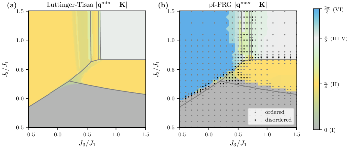
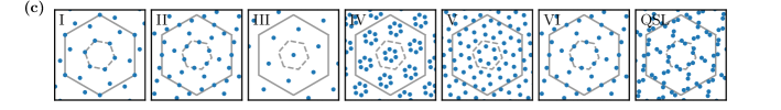
Figure 12: Unconstrained Luttinger-Tisza versus pf-FRG. (a) LT $\mathbf{q}$-vectors with minimal eigenvalue of the Fourier transformed interaction matrix. (b) Distance of the momentum where the pf-FRG structure factor is maximal $\mathbf{q}^{max}$ to the $\mathbf{K}$-point of the extended Brillouin zone. Quantum disordered regions that show no flow breakdown $(\Lambda_{c}=0)$ are marked by black dots. The gray lines are the classical phase boundaries. (c) All $\mathbf{q}$-vectors with minimal Luttinger-Tisza eigenvalue at the same parameters as shown for the quantum case (Fig. 6). The dashed and solid gray lines show the first and extended Brillouin zone, respectively.

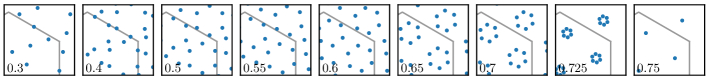
Figure 13: Ground-state $\mathbf{q}^{\mathrm{min}}$-vectors from Luttinger-Tisza evolving from phase VI to III for fixed $J_{2}/J_{1}=1$ and increasing $J_{3}/J_{1}$ (indicated in the bottom left corners). Similar to the pf-FRG results (c.f. Fig. 7), we observe a seemingly continuous evolution with no clearly distinct phases V and VI that were identified in our classical analysis.

In order to substantiate the structure factors derived from our pf-FRG calculations, especially within the incommensurate regimes where they disagree with the classical analysis, we employ the unconstrained Luttinger-Tisza (LT) approach [64, 65]. This approach studies the classical model, but relaxes the hard constraint of constant spin length on each spin to a constraint on the total spin length. Enforcing only this weak constraint enables a straight-forward Fourier transformation of the interaction matrix, and a subsequent diagonalization of the Hamiltonian in momentum space. The momenta $\mathbf{q}^{\mathrm{min}}$ with eigenvectors of minimal energy then characterize the LT ground state—a semi-classical approximation to the true ground state with an energy that serves as a lower bound on the exact ground-state energy. The fact that the LT approach works on an infinite lattice and that, as in the quantum model, spin length is not conserved, makes it a suitable tool to compare it to and corroborate the results from our pf-FRG calculation.

Figure 12 does just that, depicting the LT $\mathbf{q}$-vector with minimal eigenvalue $\mathbf{q}^{\mathrm{min}}$ (a) next to the pf-FRG ordering vectors $\mathbf{q}^{\mathrm{max}}$ of maximal structure factor intensity (b), and shows examples of the full LT ground-state $\mathbf{q}$-vectors (c) in the different phases. The most notable difference is that the LT $\mathbf{q}$-vectors are periodic with the reciprocal lattice vectors of the triangular Bravais lattice of the maple-leaf lattice, and thus fully specified by points in the first Brillouin zone (depicted by the dashed lines in Fig. 12(c)). Conversely, the pf-FRG ordering vectors are periodic on the reciprocal lattice of the smaller triangular lattice that, when depleted by 1/7, transforms into the maple-leaf lattice, and are thus fully specified by points in the extended Brillouin zone (solid gray lines). The resulting additional $\mathbf{q}$-vectors found by the LT approach are likely due to states not fulfilling the hard spin-constraint, which are therefore absent also in the structure factors from classical Monte Carlo (depicted in Fig. 2 on the right). Due to these extra momenta, phase II and phase VI are equivalent in the unconstrained LT approach, where both the pf-FRG and the classical analysis only select a subset of the LT $\mathbf{q}$-values and reveal that the phases differ even in their respective ground-state symmetry (T vs $\mathrm{D}_{3}$).

Comparing only the LT $\mathbf{q}$-vectors also present in the pf-FRG structure factor, however, the two methods agree remarkably well, both showing incommensurate $\mathbf{q}$-values in the proposed QSL regime and in between phases III and VI. Our LT calculation also predicts the smooth evolution of the structure factor from phase III to VI, as depicted in Fig. 13, resembling the pf-FRG structure factors in Fig. 7. This supports the incommensurate nature of the ground state in this parameter regime, which was not captured by our initial classical analysis.