Measuring Exploration in Reinforcement Learning
via Optimal Transport in Policy Space

Abstract

Exploration is the key ingredient of reinforcement learning (RL) that determines the speed and success of learning. Here, we quantify and compare the amount of exploration and learning accomplished by a Reinforcement Learning (RL) algorithm. Specifically, we propose a novel measure, named Exploration Index, that quantifies the relative effort of knowledge transfer (transferability) by an RL algorithm in comparison to supervised learning (SL) that transforms the initial data distribution of RL to the corresponding final data distribution. The comparison is established by formulating learning in RL as a sequence of SL tasks, and using optimal transport based metrics to compare the total path traversed by the RL and SL algorithms in the data distribution space. We perform extensive empirical analysis on various environments and with multiple algorithms to demonstrate that the exploration index yields insights about the exploration behaviour of any RL algorithm, and also allows us to compare the exploratory behaviours of different RL algorithms.

1 Introduction

In Reinforcement Learning (RL), exploration impacts the overall performance of the agent by determining the quality of experiences from which the agent learns [Zhang et al., 2019]. Exploration is the activity of searching to maximise the reward signal, and to overcome local minima (or maxima), or areas of flat rewards [Ladosz et al., 2022]. Quantifying exploration is important as it would allow evaluation of exploration qualities of different RL algorithms, and exploration strategies used in the same algorithm. However, a standardised metric to compare exploratory efforts that is algorithm-agnostic is currently absent [Hollenstein et al., 2020, Ladosz et al., 2022].

In recent years, significant advancements have been achieved in developing exploration techniques that improve learning [Bellemare et al., 2016, Osband et al., 2016, Burda et al., 2019, Eysenbach et al., 2019]. Yet, there remains a lack of consensus over approaches that can quantitatively compare these techniques across RL algorithms [Amin et al., 2021, Ladosz et al., 2022]. This is attributed to some methods being algorithm-specific [Tang et al., 2017], while others provide theoretical guarantees for tabular settings which are not extensible to non-tabular settings [Zhang et al., 2019].

The goal of exploration is to maximise the agent’s knowledge to facilitate identification of (near-)optimal policies, i.e. discovering highly rewarding sequences of state-action pairs. However, the environment dictates the difficulty of visiting all the states to identify the rewarding state-actions, which is also known as the visitation complexity [Conserva and Rauber, 2022]. An exploration strategy has to overcome this complexity to gather meaningful samples of state-actions. We quantify the relative effort of RL algorithms to overcome the visitation complexity and name it Exploration Index.

We consider that the crux of exploration effort lies in transferability, a property indicating the ease or difficulty of transferring knowledge learned across tasks [Nguyen et al., 2020, Tan et al., 2021]. During training in RL, each policy model update encountered by the agent results in a policy, and each policy generates an associated dataset of state-action pairs (aka trajectories). Therefore, a classification model learning sequentially on these datasets can be equated to the learning process of the RL agent (illustrated in Figure 1). Since the exploration strategy is responsible for policies encountered during training, we can use the relative effort of knowledge transfer induced by exploration to capture the exploratory behaviour of RL algorithm.

In Supervised Learning (SL), Alvarez-Melis and Fusi [2020] showed that transferability can be predicted based on the similarity (alternatively, distance) between task datasets. Here, we conceptualise learning in RL as a sequence of SL tasks and further leverage the optimal transport dataset distance (OTDD) developed by Alvarez-Melis and Fusi [2020]. This allows us to compute the relative exploration effort as the ratio of the overall transferability in RL over the transferability in SL.

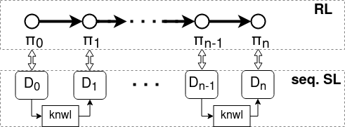
Figure 1: Illustration of RL as a sequence of SL tasks (seq. SL). Policies $\pi_{n}$ encountered during learning in RL have corresponding datasets $D_{n}$ of state-action pairs. Training a classifier successively on these datasets, while transferring knowledge (knwl), is analogous to training the RL agent.

Contributions. We introduce an Exploration Index to measure the relative effort of knowledge transfer (transferability) involved while learning in RL. We compute it by comparing similarities of datasets of state-action pairs of subsequent policies yielded during training using the optimal transport dataset distance (OTDD). Further, we perform an extensive analysis of Exploration Index across RL environments and algorithms to show its universal applicability to compare different exploration strategies used in the same RL algorithm, exploratory efforts of different RL algorithms, and hardness of different tasks.

2 Preliminaries

We introduce the basic setup of RL and Markov decision processes assumed in this paper. Then, we discuss relevant aspects of transfer learning, Wasserstein distance, and OTDD. Finally, we propose an extension of OTDD to the space of probability distributions.

RL setup. We consider an RL setup consisting of an agent interacting with an environment in discrete timesteps. At each timestep ${t}\in\mathbb{N}$, the agent observes a state ${s_{t}}$, executes an action ${a_{t}}$, and receives a scalar reward ${r_{t}}$. The behaviour of the agent is defined by a policy ${\pi}$, which maps the observed states to actions. The environment is modelled as a Markov Decision Process (MDP) with a state space $\mathcal{S}$, action space $\mathcal{A}$, transition dynamics $\mathcal{T}:\mathcal{S}\times\mathcal{A}\to\mathcal{S}$, and reward function ${r:\mathcal{S}\times\mathcal{A}\to\mathbb{R}}$. During task execution, the agent issues actions in response to states visited. Thus, we obtain a sequence of states and actions ${\tau=(s_{0},a_{0},s_{1},a_{1},...,s_{T},a_{T})}$, called a trajectory. The return, over a finite a time horizon $T$, is the discounted cumulative reward over the trajectory ${R(\tau)=\sum_{t=0}^{T}\gamma^{t}r(s_{t},a_{t})}$, with a discounting factor ${\gamma\in[0,1]}$. Note that the trajectory and return depend on the actions selected, and therefore on the policy ${\pi}$. The goal in RL is to learn a policy that maximises the expected return ${J=\mathbb{E}_{\tau\sim\pi}[R(\tau)]}$, i.e. learn a policy that generates a trajectory class $C(\pi)=\{\tau_{i}\}_{i=0}^{n\to\infty}$ corresponding to the highest possible expected return.

Transfer Learning and Task Similarity in Supervised Learning.

Transfer learning studies how the performance on a target task can be improved by knowledge learned from a source task [Tan et al., 2021]. It is known that transferring knowledge across similar tasks should be easier than across distant ones [Alvarez-Melis and Fusi, 2020]. Hence, transferability between tasks is often quantified by their similarity. High transferability implies low efforts of knowledge transfer as the model pre-trained on source data can generalise well on target task [Gao and Chaudhari, 2021].

Task similarity in SL has been studied extensively to capture transferability. For instance, various methods evaluate task similarity according to model performance [Zamir et al., 2018], embedded vector representations [Achille et al., 2019], discrepancy measures between domains [Ben-David et al., 2006], information theory [Tran et al., 2019], and optimal transport theory [Alvarez-Melis and Fusi, 2020, Gao and Chaudhari, 2021, Tan et al., 2021]. We employ a method called optimal transport dataset distance (OTDD) [Alvarez-Melis and Fusi, 2020] to determine the effort of knowledge transfer in SL tasks because it is simple and flexible to implement in practice.

Optimal Transport: Wasserstein Distance.

Optimal transport studies how to optimally shift a probability measure $u\in\mathcal{P}(\mathcal{Z})$ on a metric space $\mathcal{Z}$ to a probability measure $v\in\mathcal{P}(\mathcal{Z})$ on the same metric space. The optimal shift is quantified by Wasserstein distance [Peyré and Cuturi, 2019]. Specifically, the 2-Wasserstein distance of $u$ and $v$ is

$$W_{2}^{2}(u,v)\triangleq\min_{\pi\in\Pi(u,v)}\int_{\mathcal{Z}\times\mathcal{Z}}c(z,z^{\prime})d\pi(z,z^{\prime}).$$ (1)

Here, $\Pi(u,v)$ is the set of all transport plans between $u$ and $v$. $c(z,z\textquoteright)\in\mathbb{R}^{+}$ is the cost function quantifying the cost of transporting unit mass from $z$ to $z^{\prime}$. Note that when $\mathcal{Z}$ is endowed with a metric $d_{\mathcal{Z}}$, the cost function is $c(z,z\textquoteright)=d_{\mathcal{Z}}^{2}(z,z^{\prime})$. We use Wasserstein distance to compute OTDD.

Optimal Transport Dataset Distance (OTDD).

Let dataset $\mathcal{D}$ be a set of feature-label pairs $(x,y)\in\mathcal{X,Y}$ over a feature space $\mathcal{X}$ and label set $\mathcal{Y}$. Suppose there are two datasets $\mathcal{D_{A}}=\{(x_{A}^{i},y_{A}^{i})\}_{i=1}^{m}$ and $\mathcal{D_{B}}=\{(x_{B}^{i},y_{B}^{i})\}_{i=1}^{n}$ with $x_{A},x_{B}\in\mathcal{X}$ and $y_{A},y_{B}\in\mathcal{Y}$. The samples in these datasets are thought to be drawn from joint distributions $P_{A}(x,y)$ and $P_{B}(x,y)$. The goal of SL task is to estimate the conditional distribution model $P(y|x)$ for each dataset.

OTDD [Alvarez-Melis and Fusi, 2020] is a statistical divergence between joint distributions $P_{A}(x,y)$ and $P_{B}(x,y)$ that captures transferability from dataset $A$ to $B$. Here, transferability means the effort of learning the conditional distribution $P(y|x)$ for $\mathcal{D_{B}}$ using a model pre-trained on $\mathcal{D_{A}}$.

Following the OTDD framework, we consider the feature-label space as a metric space, i.e. $\mathcal{Z}=\mathcal{X}\times\mathcal{Y}$, and define the cost function in the 2-Wasserstein distance as

$$d_{\mathcal{Z}}((x,y),(x^{\prime},y^{\prime}))^{2}=d_{\mathcal{X}}(x,x^{\prime})^{2}+W^{2}_{2}(\alpha_{y},\alpha_{y^{\prime}}),$$ (2)

where labels are encoded as distributions over the feature space by the map $y\to\alpha_{y}(X)\doteq P(X\mid Y=y)$.

OTDD between $P_{A}(x,y)$ and $P_{B}(x,y)$, i.e. $d_{OT}(P_{A},P_{B})$, is the 2-Wasserstein distance (Equation (1)) between $P_{A}$ and $P_{B}$ computed with the cost function of Equation (2). Hereafter, we use either $d_{OT}(P_{A},P_{B})$ or $d_{OT}(\mathcal{D_{A}},\mathcal{D_{B}})$ interchangeably to denote the OTDD between joint distributions $P_{A}(x,y)$ and $P_{B}(x,y)$.

In summary, OTDD is a hierarchical Wasserstein distance that first measures the transportation cost between labels by reflecting them back to feature space, and then sums this with the cost between the input features. Note that OTDD is a metric [Alvarez-Melis and Fusi, 2020]. We use OTDD to compute overall effort of knowledge transfer (i.e. transferability) during a learning process.

2.1 Formulation: OTDD on the manifold of probability distributions

Let $P_{\theta}$ be a parameterised joint probability distribution from which samples in the dataset $\mathcal{D_{\theta}}$ are drawn, i.e. $\mathcal{D_{\theta}}=\{(x_{A}^{i},y_{A}^{i})\}_{i=i}^{m}\sim P_{\theta}$. When the parameters $\theta$ undergo a slight modification, through some update rule, the resulting distribution is denoted as $P_{\theta+d\theta}$ and samples in the dataset $\mathcal{D}_{\theta+d\theta}$ are drawn from it.

We consider a Riemannian manifold of these parameterised joint probability distributions $\mathcal{M}=\{P_{\theta}(x,y)\mid\theta\in\mathbb{R}^{N}\}$. These types of manifolds are studied in information geometry [Amari, 2010], and extended to the context of RL [Basu et al., 2020]. We endow the manifold with the OTDD metric to compute the distance between points $\theta,\theta+d\theta\in\mathcal{M}$ as $ds=d_{OT}(P_{\theta},P_{\theta+d\theta}).$ Now, suppose throughout some learning process, the parameters undergo continuous updates until a predefined convergence criterion is satisfied. This process yields a continuously differentiable curve on the manifold $\mathcal{M}$ [Gao and Chaudhari, 2021]. The length of the curve is approximated by summation of the finite distances along it [Lott, 2008].

$$C\triangleq\sum_{k=0}^{K-1}d_{OT}(P_{\theta_{k}},P_{\theta_{k+1}}).$$ (3)

$\theta_{0}$ and $\theta_{K}$ represent the initial and final parameter values before and after the learning process, respectively. Henceforth, we refer to the space of joint probability distributions on $\mathcal{M}$ equipped with the OTDD metric as the OTDD space. To define distances between the distributions induced by policies computed during RL training, we use such an OTDD space, interchangeably terming it ’policy space’.

3 Measuring Exploration in RL

In this section, we study the trajectories generated by policies as datasets, and leverage the representation of RL as sequential SLs (Figure 1) to present our exploration metric.

3.1 Episodic trajectories as datasets

We define the dataset of a policy $\pi$ as the state-action pairs originating from the set of possible trajectories obtained by playing the policy, i.e. $C(\pi)$. That is, $\mathcal{D}_{\pi}=\{(s_{(i)},a_{(i)})\}_{i=0}^{m}\in C(\pi)\subseteq\mathcal{S}\times\mathcal{A}$. These samples in the dataset are drawn from a joint distribution $P_{\pi}(s,a)$.

Proposition 3.1 Given an MDP, the joint distribution $P_{\pi}(s,a)$ is unique to policy ${\pi}$. (Proof in Appendix A)

If we are given $\mathcal{D}_{\pi}$, generated by an expert policy, we can train a policy model on it in a supervised manner, via behaviour cloning [Hussein et al., 2017]. Thus, knowing $\mathcal{D}_{\pi}$ can reduce an RL problem to an SL task.

3.2 Exploration Index

A model that learned a policy $\pi_{i}$ during pre-training can be used to generate $\mathcal{D}_{\pi_{i}}$. Suppose the objective is to learn $\pi_{j}$ using this trained model, and we are given $\mathcal{D}_{\pi_{j}}$, i.e. state-action pairs generated by $\pi_{j}$. The model can simply be retrained in a supervised manner on $\mathcal{D}_{\pi_{j}}$. Samples in $\mathcal{D}_{\pi_{i}}$ and $\mathcal{D}_{\pi_{j}}$ can be treated as support points of empirical joint distributions $\hat{P}_{\pi_{i}}$ and $\hat{P}_{\pi_{j}}$, respectively. Then the effort required for knowledge transfer in the model is $d_{OT}(\hat{P}_{\pi_{i}},\hat{P}_{\pi_{j}})$.

During training in RL, the policy model updates through $\pi_{0},\dots,\pi_{N}$. $\pi_{0}$ is usually given by randomly sampling the model parameters, and $\pi_{N}$ is achieved after convergence. Initially, $\pi_{0}$ is evaluated to generate experiences, which are then used to update the model to $\pi_{1}$. This iterative process continues until reaching $\pi_{N}$. This process is analogous to transfer learning sequentially over datasets $\mathcal{D}_{\pi_{0}},\dots,\mathcal{D}_{\pi_{N}}$ in a supervised manner.

Proposition 3.2 In the OTDD space, learning sequentially over datasets $\mathcal{D}_{\pi_{0}},\dots,\mathcal{D}_{\pi_{N}}$ using supervised learning, is a close approximation of a policy model updating through $\pi_{0},\dots,\pi_{N}$ during training in RL. (Proof in Appendix A)

If $\mathcal{D}_{\pi_{N}}$ was known a priori, then the effort of learning $\pi_{N}$ given the model for $\pi_{0}$ would be $L=d_{OT}(\mathcal{D}_{\pi_{0}},\mathcal{D}_{\pi_{N}})$, i.e. the geodesic distance on the OTDD space. However, due to exploration the policy model moves through $\pi_{0},\dots,\pi_{N}$, thus tracing a curve in the OTDD space and the overall effort of learning $\pi_{N}$ is given by Equation (3). Figure 2 illustrates learning $\mathcal{D}_{\pi_{N}}$ in a supervised manner yielding $L$ versus using RL which traces a curve $C$ mainly due to exploration.

Figure 2: Depiction of the curve $C$ traced on the OTDD space during learning in RL. The geodesic $L$ is the shortest path between initial and final points on the curve, i.e. ${P}_{\pi_{0}}$ and ${P}_{\pi_{N}}$, respectively.

By definition, $L\leq C$ since $L$ is the geodesic, i.e. shortest distance between between $\pi_{0}$ and $\pi_{N}$. We assess the effort of knowledge transfer involved in the model learning $\pi_{N}$ from initial $\pi_{0}$, using RL, in relation to simply using SL as:

$$\mathrm{EI}\triangleq\frac{C}{L}=\frac{\sum_{k=0}^{N-1}d_{OT}(\mathcal{D}_{\pi_{k}},\mathcal{D}_{\pi_{k+1}})}{d_{OT}(\mathcal{D}_{\pi_{0}},\mathcal{D}_{\pi_{N}})}$$ (4)

We define $C/L$ as the Exploration Index (EI) since it signifies the relative effort induced by exploration during learning in RL compared to learning in a supervised manner. This can be interpreted as the efficiency of exploration. An EI close to 1 indicates highly efficient exploration i.e. the exploration scheme gathers high quality experiences successfully, and hence the overall effort of knowledge transfer (transferability) is minimised.

Let $\Phi$ be the set of all possible exploration schemes for a given MDP. An optimal scheme can be defined as follows:

Definition 3.1 An optimal exploration scheme $\phi^{*}\in\Phi$ is the one that minimises, the Exploration Index, $\frac{C}{L}$.

This approach effectively links exploration and knowledge, recognizing that the objective of exploration is to maximise the agent’s knowledge such that it facilitates (near)optimal policy identification. The ability to collect high-quality experiences enhances the learning process [Zhang et al., 2019] as these data points are profoundly informative, thereby reducing unnecessary knowledge transfers.

Computing Exploration Index. The model parameters $\theta\in\mathbb{R}^{N}$ are initialised using some prior distribution $\theta_{0}\sim Q(\theta)$ (see Appendix B). The model is evaluated for $T$ number of episodes to generate state-action pairs that are collected in $\mathcal{D}_{\theta_{0}}$. The parameters are then updated using the RL algorithm’s update scheme. After every update, the model is evaluated to generate the corresponding policy’s dataset. The datasets are collected for every model update until convergence. Then we use the datasets to compute the $C$ and $L$ (as in Algorithm 1).

Algorithm 1 Computing Exploration Index (EI)

1:  Initialise model parameters $\theta\sim p(\theta)$

2:  {Perform standard RL training}

3:  for $k=0,1,\ldots,K$ model updates do

4:     for $t=0,1,\ldots,T$ episodes do

5:        Evaluate policy $\theta_{k}$ on $s_{init}$ and $s_{goal}$

6:        Store $\{(s_{(i)},a_{(i)})\}_{i=0}^{m}$ in $\mathcal{D}_{k}$

7:     end for

8:  end for

9:  $L=d_{OT}(\mathcal{D}_{0},\mathcal{D}_{K})$

10:  $C=0$

11:  for $k=0,1,\ldots,K-1$ do

12:     $C\leftarrow C+d_{OT}(\mathcal{D}_{k},\mathcal{D}_{k+1})$

13:  end for

14:  Output: $C/L$

4 Experimental Analysis

Now, we conduct extensive experiments to evaluate the usefulness of EI in capturing exploration effort and its flexibility in comparing different RL algorithms.

Experimental Setup. Our experiments consist of five deterministic 2D-Gridworld tasks with actions {up, right, down, left}. The start and goal states always located at top-left and bottom-right, respectively, except for a single task. The tasks are illustrated in Figure 3. They are selected for their simplicity, to enable clear interpretation of EI across tasks.

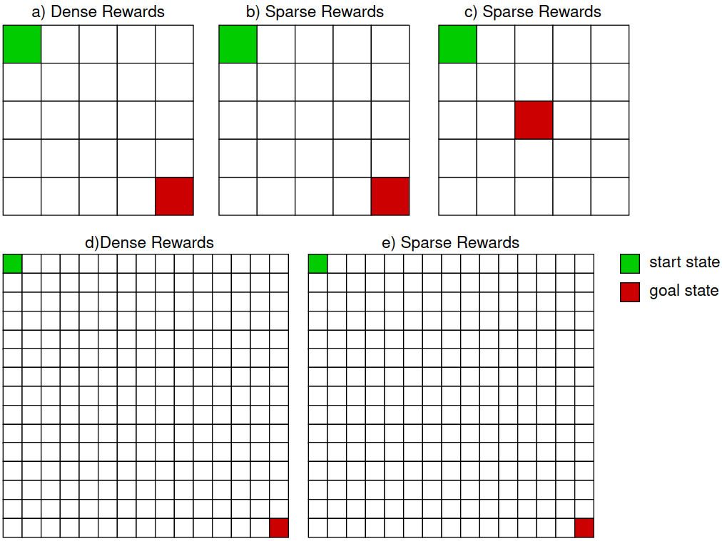
Figure 3: Five grid-world tasks with the same action space, but different rewards, state space and location of the goal state. Tasks (a) and (d) have rewards described by the L1 norm between the current and goal states $\lVert s_{c}-s_{g}\rVert_{1}$. The rest issue a reward of -0.04 at every state and 1 at the goal.

Our experiments aim to address the following questions:
1. Does EI capture expected behaviours within a simple deterministic setup employing Q-learning with $\epsilon$-greedy and decaying $\epsilon$-greedy strategies?
2. Does EI scale proportionally with the task difficulty for any specific RL algorithm?
3. How do various exploration strategies within both identical and distinct RL algorithms compare?
4. How do convergence criteria impact EIs of RL algorithms?
Summary of Results. In Section 4.1, we validate EI and show that, as expected, the EI values reduce with higher $\epsilon$ for $\epsilon$-greedy exploration. Further, EIs are lower for Q-learning with decaying $\epsilon$-greedy strategy compared to $\epsilon$-greedy strategy. Furthermore, the EI values are higher for settings with sparse rewards than with dense rewards. In Section 4.2, we show that EI scales proportionally with task difficulty, and thus, is able to reflect task difficulty on exploration. In Section 4.3, we learn that studying the variation and magnitude of segment lengths in policy space between consecutive policies, as learning progresses, gives us insight into the exploration behaviour of RL algorithms. This further enables us to decide if the exploration behaviour is suitable or unsuitable for the task. We also observe (Section 4.4) that when the convergence criterion is not strict, the EI provides complementary diagnostic information, which is not provided by convergence times of RL algorithms.

4.1 Validation of Exploration Index: Q-learning with $\epsilon$-greedy strategies

The tabular Q-learning algorithm [Watkins and Dayan, 1992] is innately deterministic. Its primary source of stochasticity is the exploration strategy, apart from the random initialization of Q-values. This attribute makes tabular Q-learning a testbed to observe the effects of exploration without any effect of external noise. $\epsilon$-greedy is a simple and undirected exploration scheme [Amin et al., 2021] that picks exploratory actions at random. Here, we validate our index employing Q-learning with $\epsilon$-greedy strategies.

We compare $\epsilon$-greedy and decaying $\epsilon$-greedy strategies, deployed in tasks (a) and (b), by examining both their EI values and convergence times (shown in Figure 4). The results are for $\epsilon=\{0.05,0.2,0.4,0.9\}$, representing a wide range from 0 to 1. We aim to evaluate the capability of the exploration strategy to stably settle at an optimal policy. The corresponding convergence criterion is satisfied when the policy model consistently yields maximum returns over 50 consecutive updates.

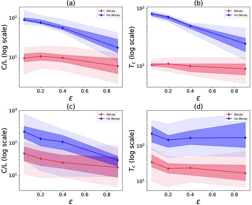
Figure 4: Plots of EI $C/L$ vs $\epsilon$ and convergence time (in steps) $T_{c}$ vs $\epsilon$ for a 5x5 grid-world. Top panels (a) and (b) depict plots in the dense rewards setting, while bottom panels (c) and (d) show plots in the sparse rewards setting. The results were averaged over 40 runs per $\epsilon$-value in each task with Q-values initialised randomly between -1 and 1. Solid lines represents the median of the data, while the darker and lighter shaded regions show the interquartile range and limits, respectively.

Figure 4 shows that the EI values are lower for the decaying $\epsilon$-greedy strategy compared to the $\epsilon$-greedy strategy. This is consistent with convergence time in describing decaying $\epsilon$-greedy as a more efficient exploration scheme which aligns with our intuition and literature [Wei, 2020]. Once the agent possesses information about the environment, it needs to exploit it and avoid recollecting known experiences [Maroti, 2019]enabling it to reach a stable and optimal policy quicker.

EI values, along with convergence times, are smaller in the dense rewards setting than the sparse rewards setting. This is consistent with literature [Ladosz et al., 2022] which highlights that employing dense rewards rather than sparse ones in reward shaping is a technique for improving exploration.

Larger $\epsilon$’s yield lower EI values for both algorithms in both tasks. This shows that in this simple task, higher exploration as opposed to exploitation is good. However, exploring extensively initially and gradually exploiting with decaying $\epsilon$ is better.

4.2 Exploration Index increases with task difficulty

Figure 5 illustrates the EI values for Q-learning with decaying $\epsilon$-greedy strategy across tasks (a) to (e) (ref. Figure 3). We chose to assess this algorithm because it is simple and yet managed to complete all the tasks. As in Section 4.1, convergence is reached when a policy model yields maximum returns over 50 consecutive updates.

We observe that the EI is lowest for task (a) and highest for task (e), as anticipated. Looking closely we can see that the medians of both EI and convergence time for task (b) are higher than for task (c). This aligns with our intuition as task (c) is a simpler version of task (b).

The results demonstrate that EI scales proportionally with task difficulty, much like convergence time. This is sensible as more challenging tasks demand greater exploration compared to simpler ones.

Figure 5: Plots depict Q-learning with decaying $\epsilon$-greedy exploration scheme across various tasks. Left: EI $C/L$ vs tasks. Right: convergence time $T_{c}$ vs tasks. The tasks (illustrated in Figure 3) are placed in order of ascending difficulty. The results were averaged over 40 runs per task with $\epsilon=0.9$.

4.3 Exploration Index for comparing exploration strategies

We utilised tasks (a), (b), and (d) of Figure 3 to evaluate the following RL algorithms: Tabular Q-learning with 1) decaying $\epsilon$-greedy, 2) $\epsilon$-greedy, 3) softmax (Boltzmann), and 4) greedy strategies, and also, 5) UCRL [Auer and Ortner, 2006], 6) SAC [Haarnoja et al., 2018, Christodoulou, 2019], and 7) DQN [Mnih et al., 2013] with decaying $\epsilon$-greedy.

The results of the experiment, depicted in Figure 6, are for the best-performing parameters for each algorithm. In Q-learning, values in the Q-table were randomly initialised between -1 and 1. Over 80 runs per algorithm in each task were performed. The considered convergence criterion is met when the policy model’s returns were consistently maximal over 5 consecutive updates, which is typically employed, but different from the 50 updates required earlier. Even with this reduced criterion, some algorithms had difficulty succeeding (see Table 1). In these cases, we set a cut-off training time of 500 episodes (with 60 steps per episode) and still computed the EI (see Methods in Appendix B) to differentiate exploration in the various algorithms even without convergence.

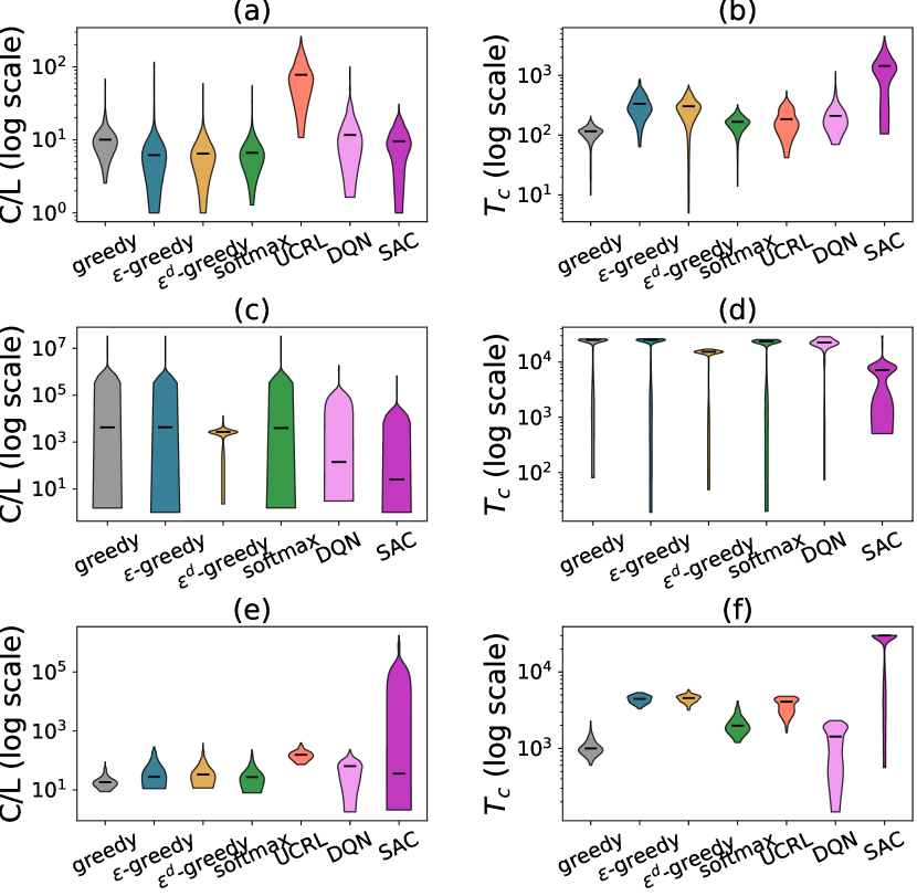
Figure 6: Violin plots of EI $C/L$ and convergence time $T_{c}$ vs RL algorithms in gridworld tasks. Panels (a) and (b) are for a 5x5 dense rewards task, (c) and (d) for 5x5 sparse rewards task, and (e) and (f) for 15x15 dense rewards task. The first four RL algorithms are tabular Q-learning based with different exploration schemes, while the rest are assorted RL algorithms. We plot mean values and distributions of the data collected over 80 runs per algorithm for each task.

Task (a) 5x5 grid and dense rewards. We see that the decaying $\epsilon$-greedy, $\epsilon$-greedy and softmax algorithms equivalently have the lowest EI values. The trio is followed by SAC, greedy and DQN, respectively. UCRL has the highest EI. However, greedy has the best convergence time and SAC the worst in comparison to the rest. This highlights that the relative effort of knowledge transfer does not necessarily correlate with the convergence time across algorithms. This can be well explained by contrasting exploration behaviours of UCRL, SAC, and Q-learning greedy as in Figure 7.

The high values of ‘segment lengths’, i.e. OTDD distances in policy space between consecutive policy updates, at the start of learning (Figure 7 (a)), reveal that UCRL initially explores aggressively by traversing broader within the OTDD space, then gradually reduces coverage distance, and then settles into a rather high segment length between successive policies. In this manner, UCRL expends notable effort to reach optimality quicker. However, the high segment length ($\sim 1.0$) even after settling, compared to other algorithms in Figure 7 suggests that the exploration strategy is less inclined to stabilise reliably at an optimal policy, i.e. it is likely to escape from the optimal policy region, wander into other areas, before eventually returning or encountering another optimal policy (see Figure 9 as well). Such an exploration strategy can be called diverse since it explores a wide range of policies without honing in on the most promising one.

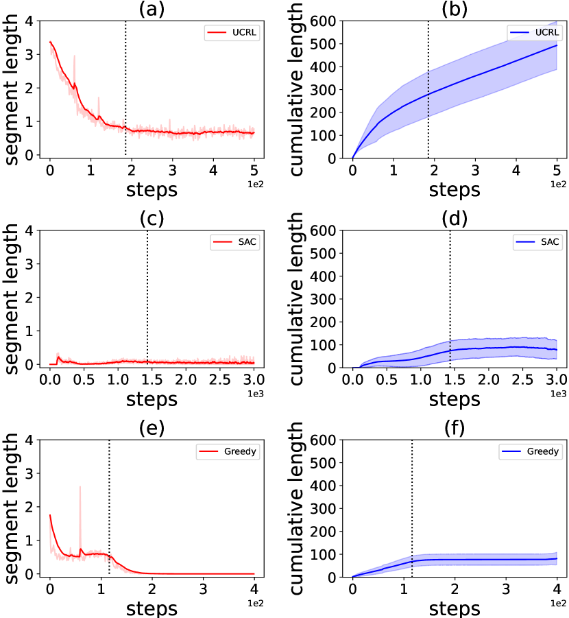
Figure 7: The behaviour of the ’segment length’ (distance between consecutive policies on the OTDD space) over time for RL algorithms UCRL, SAC, and Q-learning greedy on the 5x5 dense rewards task. The cumulative length plots demonstrate how the segment length accrues across time to determine the length of the curve $C$ on the OTDD space. The vertical dotted line represents the mean convergence time averaged over 80 runs. For segment length plots, the solid line represents a smoothed rendition of the noisy mean curve, shown shaded. For cumulative length plots, the solid line depicts the mean curve and the shaded areas indicate the range of standard deviation values.

By contrast, Figure 7 (b) shows that while the greedy strategy at first explores widely due to random Q-value initialization, it rapidly narrows down its coverage distance as the Q-values are updated following a greedy strategy. Once it finds an optimal policy, it ceases further exploration. This strategy prioritises precision in finding a promising policy and overlooks the exploration of alternative policies. The drawback is that it might miss out on potentially superior policies in unexplored regions. This type of exploration can be described as precise. It conserves effort of knowledge transfer and time by honing in on the most promising policy. Such a behaviour was also observed in the other exploration strategies in Q-learning (shown in Appendix C).

Rather than starting with wide traversals, SAC maintains a low search distance fairly consistently (shown in Figure 7 (c)), and thus, conserving effort but sacrificing time. The exploration strategy in SAC can hone in on a promising policy, search within its region for other policies, and only deviate when nearby policies are similar to the promising one. It is therefore likely to alternate between equally promising policies provided they are clustered closely. The exploration strategy in SAC is somewhere between diverse and precise.

Task (b) 5x5 grid and sparse rewards. We increased the task difficulty by discarding reward shaping. As seen in panels (c) and (d) of Figure 6, the EI values, and also convergence times, are an order of magnitude or two higher compared to the 5x5 dense rewards task.

All the exploration strategies used in the Q-learning algorithm had low success rates here as seen in Table 1. Since the strategies did not traverse very far in the policy space, often not reaching optimal policies, they had low geodesic distances $L$, leading to a large $C/L$. The convergence times in these cases reached the cut-off limit of learning time. However, the EI $C/L$ continues to be informative about the exploration effort, even when the algorithm does not succeed, enabling it to be used as a diagnostic tool.

SAC had the highest success rate followed closely by DQN, while the others have poor success rates. We observe that the convergence time can be misleading in providing information about exploration efficiency, while the EI is not. In the case of DQN, its success rate aligns with the EI value while the convergence time would have suggested it is as poor as others.

As expected, deep learning algorithms SAC and DQN outperformed Q-learning algorithms, and thus, are consistent with literature Mnih et al. [2013]. The exploration strategies in Q-learning seem to have the same EI median. However, decaying $\epsilon$-greedy has data points concentrated around the median, while others seem to be widely distributed. The wide distribution of the data indicates that there are instances where optimal policies were successfully reached as well as not, contrasting with distributions exhibiting low dispersion.

Algorithm	[5x5] D	[5x5] S	[15x15] D
Decaying $\epsilon$-greedy	100.0%	5.0%	88.7%
$\epsilon$-greedy	100.0%	15.0%	96.2%
Greedy	100.0%	13.0%	100.0%
UCRL	100.0%	-	92.5%
Softmax	100.0%	15.0%	92.5%
DQN	100.0%	83.0%	77.4%
SAC	100.0%	98.0%	20.8%

Table 1: The success rates of exploration schemes on tasks (a) 5x5 dense rewards, (b) 5x5 grid-world sparse rewards, and (d) 15x15 grid-world with dense rewards. The success criterion was formulated to be satisfied when the model policy consistently yields maximum returns for the task across a span of 50 successive updates. UCRL was not tested on task (b) since it cannot handle transient states Jaksch et al. [2010], often found in sparse reward settings.

Task (d) 15x15 grid and dense rewards. Here, we increased the task difficulty by increasing the state space. We see in Figure 6 (e) and (f), that SAC is the worst-performing algorithm. Although its EI has a small median, the wide distribution highlights instances of failure to reach optimal policies. Its poor performance was unexpected, and in this task, it seems that starting off with exploring widely has an advantage as algorithms with this exploration strategy performed well (see Table 1 for the success rates).

In this task, Q-learning with greedy strategy seems to be a superior algorithm, followed by other Q-learning algorithms. Although UCRL had better success rate than DQN, it scored worse in EI and convergence time. This means, UCRL takes more time and effort to consistently attain optimal policies. We notice that both EI and convergence time cannot always predict success. However, they are useful in understanding exploration behaviour, particularly EI.

In summary, we see that convergence time lacks the gradation to concisely convey the algorithms’ ability to reach the optimal policy, while EI does (Figure 6 (c)-(d)). Also, with segment length plots, we can analyse the inherent exploratory behaviour of an RL algorithm for a task.

4.4 Effects of Convergence Criterion on Exploratory Index

We set a stricter convergence criterion of 50 consecutive policy updates with maximal returns in Section 4.2 compared to the more typical convergence over 5 policy updates (Section 4.3), yielding EI values for 5x5 dense rewards task for the decaying $\epsilon$-greedy that do not match across the two cases as seen in Figures 5 and 6. Here, we test all the aforementioned RL algorithms on the 5x5 dense rewards task (a) across these two convergence criteria.

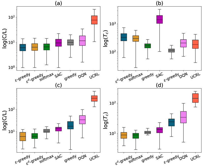
Figure 8: Plots demonstrate the relationship between EI and convergence time of various algorithms across convergence criteria of varying strictness. (a) and (b) are for a span of 5 consecutive policy model updates yielding maximum returns, while (c) and (d) are for 50. The task is a 5x5 gridworld with dense rewards.

In Figure 8(c) and (d), the EI strongly correlates with convergence time when the convergence criterion is stricter, but doesn’t correlate as much under the less restrictive typical convergence criterion (Figure 8(a) and (b)).

With a weaker criterion, a diverse exploration strategy with high EI may reach an optimal policy fast i.e. with low convergence time. With a stricter criterion, it may need to meander in and around the space of optimal policies till it settles stably within the optimal region, leading to a higher convergence time and greater correlation between EI and convergence time. A more precise strategy with lower EI will in any case settle quicker as discussed in Section 4.3. These behaviours are illustrated in Figure 9, where $C_{1}$ and $C_{2}$ denote trajectories in the OTDD space taken by a diverse exploration strategy (e.g. UCRL) and a precise exploration scheme (e.g. decay $\epsilon$-greedy), respectively.

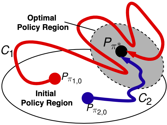
Figure 9: Illustration of exemplary exploration behaviours of exploration strategies with diverse and precise characteristics. Curve $C_{1}$ shows how typically diverse exploration behaves in comparison to precise exploration represented by curve $C_{2}$.

5 Discussion

Our work is an attempt to theoretically and quantitatively understand exploration in RL. We tackle this by introducing Exploration Index (EI), which contrasts learning in RL against learning in SL. This helps us identify exploration efficiency as the relative effort of knowledge transfer involved during learning in RL. With EI, we are able to compare exploration strategies from both tabular and non-tabular RL algorithms. Using this concept, we were able to study and extract insights about the exploration behaviour of various schemes and also witness the effect of the strictness of convergence criterion on exploration. Not only is that EI is based on sound theory, but we also provide several empirical evaluations to demonstrate its usefulness in practice.

It should be noted that EI presupposes that for any RL algorithm, exploration is the primary source of stochasticity contributing to its path within the OTDD space. This assumption is true for deterministic RL algorithms but may require careful consideration for algorithms that include other sources of noise, such as stochastic gradient descent (e.g. SAC and DQN). Future work could assess when exploration is the dominant source of stochasticity in non-deterministic RL algorithms, or various mitigations otherwise.

Briefly list author contributions. This is a nice way of making clear who did what and to give proper credit. This section is optional.

H. Q. Bovik conceived the idea and wrote the paper. Coauthor One created the code. Coauthor Two created the figures.

Measuring Exploration in Reinforcement Learning
via Optimal Transport in Policy Space (Supplementary Material)

This Supplementary Material should be submitted together with the main paper.

Appendix A Proof Details

Proof of Proposition 3.1. Suppose that the environment transitions and the policy are stochastic, then the trajectory distribution is

$$p(\Gamma|\pi)=\rho_{0}(s_{0})\Pi_{t=0}^{T}p(s_{t+1}|s_{t},a_{t})\pi(a_{t}|s_{t}),$$ (5)

where $\Gamma$ is the space of possible trajectories, $\tau_{i}\sim p(\Gamma|\pi)$ and $C(\pi)=\{\tau_{i}\}_{i=0}^{n\to\infty}$. If two trajectory distributions $p(\Gamma|\pi_{1})$ and $p(\Gamma|\pi_{2})$ produce the same dataset $C(\pi)$, then $p(\Gamma=\tau|\pi_{1})=p(\Gamma=\tau|\pi_{2})$ for all $\tau$. However, $p(\Gamma|\pi_{1})$ and $p(\Gamma|\pi_{2})$ are only truly distinct distributions if $\pi_{1}\neq\pi_{2}$. Therefore, there must exist at least one outcome $\tau$ for which $p(\Gamma=\tau|\pi_{1})\neq p(\Gamma=\tau|\pi_{2})$. This contradiction proves that two distinct policies cannot produce the same trajectory class $C(\pi)$, and if $C(\pi)$ is unique to the policy ${\pi}$, then so is $P_{\pi}(s,a)$.

Proof of Proposition 3.2. On the OTDD space, the true, i.e. unapproximated distance between consecutive policies $\pi_{i}$ and $\pi_{i+1}$ after an update is $d_{OT}(P_{\pi_{i}},P_{\pi_{i+1}})$. This is induced by $i^{th}$ RL policy update. While in supervised learning, we estimate the distance using datasets of policies, i.e. approximated joint distributions, using $d_{OT}(\hat{P}_{\pi_{i}},\hat{P}_{\pi_{i}+1})$. Therefore,

$$|d_{OT}(P_{\pi_{i}},P_{\pi_{i+1}})-d_{OT}(\hat{P}_{\pi_{i}},\hat{P}_{\pi_{i+1}})|\leq\epsilon$$ (6)

where $\epsilon$ is some small value. By summing sequentially through policies encountered during RL training:

$$\sum_{i}|d_{OT}(P_{\pi_{i}},P_{\pi_{i+1}})-d_{OT}(\hat{P}_{\pi_{i}},\hat{P}_{\pi_{i+1}})|\leq k\epsilon$$ (7)

Since from reverse triangle inequality we know,

$$\left|\sum_{i}d_{OT}(P_{\pi_{i}},P_{\pi_{i+1}})-\sum_{i}d_{OT}(\hat{P}_{\pi_{i}},\hat{P}_{\pi_{i+1}})\right|\leq\sum_{i}|d_{OT}(P_{\pi_{i}},P_{\pi_{i+1}})-d_{OT}(\hat{P}_{\pi_{i}},\hat{P}_{\pi_{i+1}})|$$ (8)

Therefore

$$\left|\sum_{i}d_{OT}(P_{\pi_{i}},P_{\pi_{i+1}})-\sum_{i}d_{OT}(\hat{P}_{\pi_{i}},\hat{P}_{\pi_{i+1}})\right|\leq k\epsilon$$ (9)

This means as the size of the dataset increases $\hat{P}_{\pi}\to P_{\pi}$, then $\sum_{i}d_{OT}(\hat{P}_{\pi_{i}},\hat{P}_{\pi_{i+1}})\to\sum_{i}d_{OT}(P_{\pi_{i}},P_{\pi_{i+1}})$.

Appendix B Methods

B.1 Results in Figures

Model parameter initialisation. We initialised model parameters for deep learning RL algorithms like DQN and SAC by uniformly sampling weight values between $-3\cdot 10^{-4}$ and $3\cdot 10^{-4}$ and the biases at $0$. For tabular Q-learning algorithms, we randomly initialized the Q-values between $-1.0$ and $1.0$.

Results in Figure 4. To determine results in Figure 4, we worked with $\epsilon=\{0.05,0.2,0.4,0.9\}$. For each $\epsilon$ value we ran 40 training trials and quantified the numerical data as displayed in the figures. With decaying $\epsilon$-greedy, we begin with the given $\epsilon$-value and exponentially using Equation 10 below. The convergence criterion was met when the policy model consistently produced maximal returns over 50 updates.

$$\epsilon=max\{0.9999\cdot\epsilon,0.0001\}$$ (10)

Results in Figure 5. Q-learning with decaying $\epsilon$-greedy was employed on the grid-world tasks (Figure 3) for a convergence criterion of 50 model updates with maximum returns. We selected $\epsilon=0.9$ and aggregated the result on over 40 training trials.

Results in Figure 6 and Table 1 Q-learning with greedy has its Q-values updated based on a greedy (exploitative) strategy. For panels (a) and (b), all algorithms achieved $100\%$ success rate unlike in other panels. The success rate was computed based on the number of training trials each algorithm met the convergence criterion of producing maximum returns over 5 consecutive updates. For $\epsilon$-greedy and decaying $\epsilon$-greedy $\epsilon=0.9$ was utilized, and $\tau=2.0$ and $\delta=0.1$ for Softmax(Boltzmann) and UCRL, respectively. The $\alpha$ parameter for SAC was autotuned using the approach in [Haarnoja et al., 2019] along with hyperparameters described in Table 2. While DQN began with $\epsilon=1.0$ and the value decayed using Equation 10. Table 13 shows hyperparameters for DQN.

For panels (c) - (f), there were instances when the geodesic length between the initial and final policies $L=d_{OT}(\mathcal{D}_{\pi_{0}},\mathcal{D}_{\pi_{N}})$ was equal to 0. This happens usually occurs when the algorithm could not reach an optimal policy and randomly landed on the initial policy. To avoid infinite EI values we added $10^{-3}$ on all $L$ values in our implementation. This provides reasonable large numbers.

Table 2: SAC Hyperparameters.

Parameter	Value
optimizer	Adam Kingma and Ba [2017]
learning rate	$5\cdot 10^{-4}$
discount($\gamma$)	0.99
replay buffer size	$10^{4}$
number of hidden layers (all networks)	1
number of hidden units per layer	32
number of samples per minibatch	64
nonlinearity	ReLU
entropy target	-4
target smoothing coefficient ($\tau$)	0.01
target update interval	1
gradient steps	1
initial exploration steps
before model starts updating	500

Table 3: DQN Hyperparameters.

Parameter	Value
optimizer	Adam Kingma and Ba [2017]
learning rate	$5\cdot 10^{-2}$
discount($\gamma$)	0.99
replay buffer size	$10^{4}$
number of hidden layers (all networks)	1
number of hidden units per layer	32
number of samples per minibatch	64
nonlinearity	ReLU
target smoothing coefficient ($\tau$)	0.001
target update interval	1
gradient steps	1
initial exploration steps
before $\epsilon$ decays	1500

Results in Figure 7 The plots show segments length $ds=d_{OT}(P_{\theta},P_{\theta+d\theta})$ vs time-steps. While the cumulative plots show accumulation of the segment lengths over time. The results in segment plots were smoothed using exponential smoothing with smoothing factor of 0.9. The plots are were made, similarly to Figure 6, with over 80 training trials for the 5x5 dense rewards task.

Results in Figure 8 We used the same approach as in Figure 6, however the convergence criteria were 5 and 50, respectively. The task was a 5x5 grid-world with dense rewards.

B.2 Calculations

OTDD. To compute the OTDD given that we have collected datasets $\mathcal{D}_{\pi}=\{(s_{(i)},a_{(i)})\}_{i=0}^{m}$, we define a set of states with action $a$ in $\mathcal{D}_{\pi}$ as $\mathcal{N}_{\mathcal{D}_{\pi}}(a)=\{s\in\mathcal{S}\mid(s,a)\in\mathcal{D}\}$ with cardinality $n_{a}$. This is used as a finite sample to define distribution that encodes action $a$ as

$$\alpha_{a}=\frac{1}{n_{a}}\sum_{s\in\mathcal{N}_{\mathcal{D}_{\pi}}(a)}\delta_{s}$$ (11)

We then precompute and store in memory action-to-action pairwise Wasserstein distances $W_{2}(\alpha_{a},\alpha_{a^{\prime}})$ using an off-the-shelf optimal transport solver toolbox POT [Flamary et al., 2021]. The cost function used was L1-norm (cityblock or Manhattan distance) since the tasks are grid-worlds restricted to vertical and horizontal movements between states. Following Equation (2), OTDD between two policy distributions is

$$d^{2}_{OT}(\hat{P}_{\pi_{i}},\hat{P}_{\pi_{j}})=\min_{\gamma\in\Gamma(\hat{P}_{\pi_{i}},\hat{P}_{\pi_{j}})}\int_{\mathcal{S}\times\mathcal{A}}\left(\lVert s-s^{\prime}\rVert^{2}_{1}+W^{2}_{2}(\alpha_{a},\alpha_{a^{\prime}})\right)d\gamma((s,a),(s^{\prime},a^{\prime}))$$ (12)

Equation (12) is also solved using the toolbox POT, while action-to-action pairwise distances are retrieved from memory on-demand. Due to the simplicity of our tasks, an Earth Movers distance algorithm [Peyré and Cuturi, 2019] in OT is used.

Appendix C Additional experimental results

This section encompasses segment length and cumulative length plots of Q-learning with $\epsilon$-greedy (Figure 10), decaying $\epsilon$-greedy (Figure 11), and Softmax (Figure 12) strategies, along with DQN (13).

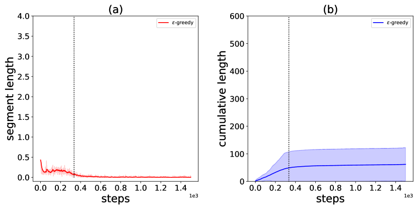
Figure 10: These plots show the behaviour of the segment length over time for Q-learning with $\epsilon$-greedy strategy. The vertical dotted line represents the mean convergence time averaged over 80 runs. For segment length plots, the solid line represents a smoothed rendition of the noisy mean curve, which is shaded. While for cumulative length plots, the solid line depicts the mean curve and the shaded areas indicate the range of standard deviation values.

Figure 11: These plots show the behaviour of the segment length over time for Q-learning with decaying $\epsilon$-greedy strategy.

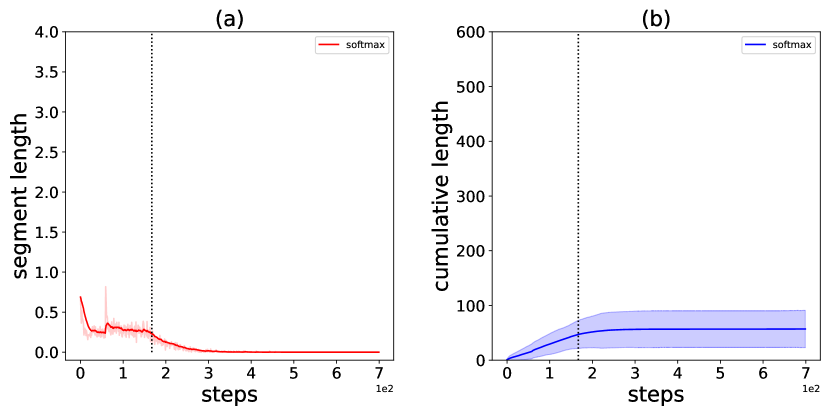
Figure 12: These plots show the behaviour of the segment length over time for Q-learning with softmax strategy.

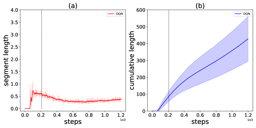
Figure 13: These plots show the behaviour of the segment length over time for DQN.