Regression graphs and sparsity-inducing reparametrizations

Summary.

Motivated by the important statistical role of sparsity, the paper uncovers four reparametrizations for covariance matrices in which sparsity is associated with conditional independence graphs in a notional Gaussian model. The intimate relationship between the Iwasawa decomposition of the general linear group and the open cone of positive definite matrices allows a unifying perspective. Specifically, the positive definite cone can be reconstructed without loss or redundancy from the exponential map applied to four Lie subalgebras determined by the Iwasawa decomposition of the general linear group. This accords geometric interpretations to the reparametrizations and the corresponding notion of sparsity. Conditions that ensure legitimacy of the reparametrizations for statistical models are identified. While the focus of this work is on understanding population-level structure, there are strong methodological implications. In particular, since the population-level sparsity manifests in a vector space, imposition of sparsity on relevant sample quantities produces a covariance estimate that respects the positive definite cone constraint.

Some key words: Directed acyclic graph; Exponential map; General linear group; Iwasawa decomposition; Matrix logarithm; Sparsity.

1. Introduction

Sparsity, the existence of many zeros or near-zeros in some domain, plays at least two roles in statistics depending on context: to aid interpretation of a high-dimensional interest parameter; and to prevent accumulation of estimation error associated with a high-dimensional nuisance parameter. There is now a large literature concerned with enforcing sparsity on sample quantities, having assumed that the corresponding population-level object is sparse. For an extensive account, see Wainwright (2019).

The present paper barely touches on sample quantities. It is concerned, in the specific context of covariance estimation, with the suggestion (Battey, 2023) that one might systematically induce sparsity on population-level quantities through reparametrization. A precursor to the idea, although the authors did not use this terminology, is parameter orthogonalization (Cox & Reid, 1987). The latter entails a traversal of parametrization space by solving a system of partial differential equations, constructed in such a way that interpretation of the interest parameter is retained, and such that in the new parametrization, the nuisance parameter is orthogonal to the interest parameter in the sense of e.g. Jeffreys (1948, pp. 158,184). In other words, the nuisance parameter is redefined in such a way that it induces sparsity on the relevant block of the Fisher information matrix, a population-level object, thereby reducing its role. Any interpretation of the original nuisance parameter is sacrificed in favour of a more reliable inference for the interest parameter. Inducement of population-level sparsity does not seem to have received subsequent attention until the recent examples highlighted by Battey (2023), although it could be argued that the development of Gaussian graphical models (e.g. Lauritzen, 1996; Cox & Wermuth, 1996) is in this vein, together with the important work on graphical modelling for extremes by Engelke & Hitz (2020).

The main question we seek to address is whether, for a given covariance matrix, not obviously sparse in any domain, a sparsity-inducing reparametrization can be deduced. Battey (2017) and Rybak & Battey (2021) provided a proof of concept for this idea. Their position was that covariance matrices and their inverses are often nuisance parameters, and it is therefore arguably more important that the sparsity holds to an adequate order of approximation in an arbitrary parametrization, than that the sparse parametrization has interpretable zeros. In the case of Gaussian graphical models, the precision matrix is the interest parameter by virtue of the interpretability ascribed to its zeros. Thus, both aspects are of interest and are addressed here. A third type of situation, to which the present paper does not contribute, is when the covariance matrix is a nuisance parameter that has a known structure up to a low-dimensional parameter. This situation is common in some settings, for instance in the analysis of split-plot or Latin square designs with block effects treated as random. The appropriate method of analysis is then residual maximum likelihood (Patterson & Thompson, 1971) or modifications thereof, which implicitly resolves the residual space into suitable orthogonal subspaces associated with a standard analysis of variance, when one exists; see e.g. Bailey (2008) for analysis of variance with random block effects, and McCullagh (2023, Ch. 8) for a discussion of residual maximum likelihood.

The contribution of the work to be presented is manifold. New geometric insight motivates reparametrizations of the set of covariance matrices. Specifically, since every full-rank covariance matrix is positive definite, which in turn is invertible, we associate any positive definite matrix with the equivalence class of invertible matrices that are orthogonally related. The set of such equivalence classes is thus identified with the set of positive definite ones, and the set of full-rank covariance matrices is thereby viewed as a parametrized homogeneous manifold of the general linear group of invertible matrices.

Every invertible matrix can be decomposed in many ways as (a combination of) rotation, scale and shear matrices that represent geometric rigid and non-rigid transformations of a real vector space. From the Iwasawa and Cartan decompositions of the general linear group, invertible matrices are given coordinates based on infinitesimal versions of such transformations, which, modulo the aforementioned equivalence relation, can be used to parametrize positive definite matrices. The unifying perspective so obtained recovers the examples of Battey (2017) and Rybak & Battey (2021) as special cases, while also pointing to new parametrizations whose applicability appears much broader in view of their graphical models interpretation under a notional Gaussian graphical model. Through these insights, the work uncovers an information geometry of Gaussian graphical models via the partial Iwasawa coordinates of the general linear group, which is naturally compatible with the information geometry of Gaussian models (Rao, 1945; Jeffreys, 1946); see §8.2.

While the focus of this work is deterministic, we highlight recent important work by Zwiernik (2023), whose complementary focus on estimation covers the matrix logarithmic sparsity model of Battey (2017) and, more generally, models with linear restrictions on spectral functions of the covariance matrix. While the extension of the Zwiernik (2023) work to the new parametrizations is not immediate, his framework, in respecting the geometry of covariance spaces, is extremely appealing.

Section 2.3 details the geometric insight leading to the reparametrizations of §3, and §2.2 gives a formal treatment of reparametrization. While rigour necessitates such a formalization, which repays careful reading, the key ideas of §3 are understandable from first principles and could be tackled directly, although with some relinquishment of insight. The main results and statistical insights are in §4 and §5.

2. Background

2.1. Notation

The following subsets of the vector space $\textsf{M}(p)$ of $p\times p$ real matrices are extensively referenced; most of them are matrix Lie groups with matrix multiplication as the group operation: the symmetric matrices $\textsf{Sym}(p)$; the skew symmetric matrices $\textsf{Sk}(p)$; the general linear group of nonsingular matrices $\textsf{GL}(p)$; the group of orthogonal matrices $\textsf{O}(p)\subset\textsf{GL}(p)$; the rotation group of special orthogonal matrices $\textsf{SO}(p)\subset\textsf{O}(p)$ with determinant $+1$; the symmetric positive definite matrices $\textsf{PD}(p)\subset\textsf{GL}(p)$; the group of diagonal matrices $\textsf{D}(p)$; the group of permutation matrices $\textsf{P}(p)\subset\textsf{O}(p)$; the group of lower triangular matrices with arbitrary diagonal entries $\textsf{LT}(p)$; the group of lower triangular matrices with unit diagonal entries $\textsf{LT}_{\textsf{u}}(p)\subset\textsf{LT}(p)$; the group of strictly lower triangular matrices $\textsf{LT}_{\textsf{s}}(p)\subset\textsf{LT}(p)$. Versions of the upper triangular matrices $\textsf{UT}(p)$ are defined analogously, and versions of $\textsf{D}(p)$ and $\textsf{LT}(p)$ with positive diagonal elements are differentiated using the subscript $+$. We denote by $\textsf{V}(p)$ a generic vector subspace of $\textsf{M}(p)$ and by $\textsf{Cone}_{p}\subset\textsf{Sym}(p)$ the (interior of a) convex cone within $\textsf{Sym}(p)$ (excluding the origin), an open subset of $\textsf{Sym}(p)$. We denote by $\oplus$ and $\otimes$, respectively, the direct sum and product of two vector spaces; we also use $\oplus$ and $\otimes$ for the kronecker sum and kronecker product when the context is clear.

With $\operatorname{\mathbf{vec}}:\textsf{Sym}(p)\rightarrow\mathbb{R}^{p^{2}}$ the vectorization map taking a symmetric matrix to a $p^{2}$-dimensional column vector, define the half-vectorization map

$$\operatorname{\mathbf{vech}}:\textsf{Sym}(p)\to\mathbb{R}^{p(p+1)/2},\quad\operatorname{\mathbf{vech}}(x):=A\operatorname{\mathbf{vec}}(x),$$

where the matrix

$$A:=\sum_{i\geq j}(u_{ij}\otimes e_{j}^{{\rm T}}\otimes e^{{\rm T}}_{i})\in\mathbb{R}^{p(p+1)/2\times p^{2}}$$

picks out the upper triangular part of the vectorization, and $u_{ij}$ is a $p(p+1)/2$-dimensional unit vector with 1 in position $(j-1)p+i-j(j-1)/2$ and 0 elsewhere. Its inverse

$$\mathbb{R}^{p(p+1)/2}\ni x\mapsto\operatorname{\mathbf{vech}}^{-1}(x):=(\operatorname{\mathbf{vech}}(I_{p})^{{\rm T}}\otimes I_{p})(I_{p}\otimes x)\in\mathbb{R}^{p\times p}$$

exists through the Moore-Penrose inverse of $A$. Here and elsewhere, $e_{1},\ldots,e_{d}$ denote the canonical basis vectors for $\mathbb{R}^{d}$, where $e_{i}\in\mathbb{R}^{d}$ is a vector with 1 for its $i$th component and zero elsewhere.

2.2. $\textsf{PD}(p)$ as a parametrized manifold and sparsity

The set of $p\times p$ covariance matrices can be identified with the convex cone $\textsf{PD}(p)$. By viewing $\textsf{PD}(p)$ as a submanifold of the vector space of $p\times p$ real matrices we can construct a parametrization that makes it a parametrized manifold. Consider the injective map

$$f:\textsf{Cone}_{p}\to\mathbb{R}^{p^{2}},\quad x\mapsto f(x):=\operatorname{\mathbf{vech}}^{-1}(x)$$

that maps a point in $\textsf{Cone}_{p}$ to a positive definite matrix within $\mathbb{R}^{p^{2}}$. At every point $x\in M$, the derivative $Df(x)$ is injective where its matrix representation is of rank $p(p+1)/2$. Then $f(\textsf{Cone}_{p})=\textsf{PD}(p)\subset\mathbb{R}^{p^{2}}$ and we say that $f$ is a parametrization of $\textsf{PD}(p)$. A reparametrization of $\textsf{PD}(p)$ corresponds to an injective map $h:N\to\mathbb{R}^{p^{2}}$ from a domain $N$ with non-singular derivative such that there is a diffeomorphism $\psi:N\to\textsf{Cone}_{p}$ with $h=f\circ\psi$. The derivative condition ensures that $N$ is of dimension $p(p+1)/2$. The two parametrizations $f$ and $h$ are said to be equivalent since $f(\textsf{Cone}_{p})=h(N)=\textsf{PD}(p)$, and $h$ is a reparametrization of $f$ (and vice versa). The commutative diagram in the left half of Figure 1 illustrates the type of reparametrization used in this paper.

Figure 1. The map $h$ is a reparameterisation of $\textsf{PD}(p)$ initially parameterised using $f=\operatorname{\mathbf{vech}}^{-1}$. In contrast, map $g$ parametrizes a statistical manifold of parametric probability measures.

In contrast, the statistical model or manifold is determined via an injective map $g:\textsf{PD}(p)\to\big{\{}\mathbb{P}_{\Gamma}:\Gamma\in\textsf{PD}(p)\big{\}}$ that maps a covariance matrix $\Gamma$ to a parametric probability measure $\mathbb{P}_{\Gamma}$ on some sample space. Every $\Sigma$ is obtained from unique points in $\textsf{Cone}_{p}$ and $N$, and the statistical model given by $g$ is impervious to reparametrization of the manifold $\textsf{PD}(p)$. Reparametrization of the statistical model amounts to applying a diffeomorphism $\textsf{PD}(p)\to\textsf{PD}(p)$ such that correspondences $\Gamma\mapsto\mathbb{P}_{\Gamma}$ change but not the image $g(\textsf{PD}(p))$. This form of reparametrization is not considered in the present work.

A sparse matrix $\Sigma\in\textsf{PD}(p)$ with respect to the parametrization $f$ is the image under $\operatorname{\mathbf{vech}}^{-1}$ of a sparse vector $\sigma\in\textsf{Cone}_{p}$ coordinatized in the standard basis of $\mathbb{R}^{p(p+1)/2}$: zero components of $\sigma$ manifest as zero elements in $\Sigma$. The structure of sparsity in $\Sigma$ with respect to the domain $N$ depends on how $N$ is coordinatized and the map $h$. We will use sparsity to refer to the domain or to the range of a parametrization interchangeably, with context disambiguating the two.

2.3. $\textsf{PD}(p)$ as a homogeneous space of $\textsf{GL}(p)$

Crucial to our approach to reparametrization is the close relationship between the general linear group $\textsf{GL}(p)$ of invertible matrices and $\textsf{PD}(p)$. Concepts from group theory relevant to this paper can be found in Appendix A. Note that $X^{{\rm T}}X$ is positive definite for every $X\in\textsf{GL}(p)$, and the map $X\mapsto X^{{\rm T}}X$ is invariant to the action $(X,O)\to OX$ for $O\in\textsf{O}(p)$ of the orthogonal group. A positive definite matrix $S$ can be transformed to any other under the transitive action

$$(X,S)\to XSX^{{\rm T}},\quad X\in\textsf{GL}(p),\thickspace S\in\textsf{PD}(p)$$

of $\textsf{GL}(p)$, and $\textsf{PD}(p)$ is hence a homogeneous space: a differentiable manifold with a transitive differentiable action of $\textsf{GL}(p)$. For example, between any pair $S_{1},S_{2}\in\textsf{PD}(p)$ the invertible matrix $X=S_{2}^{1/2}S_{1}^{-1/2}$ transforms $S_{1}$ to $S_{2}$ under the above action. The orthogonal group $\textsf{O}(p)$ is the stabilizer of $X=I_{p}$ and fixes $X\in\textsf{GL}(p)$, and we thus obtain the identification with $\textsf{GL}(p)$ via the group isomorphism

$$\textsf{PD}(p)\cong\textsf{GL}(p)/\textsf{O}(p),$$

where $\textsf{GL}(p)/\textsf{O}(p)$ is the set of equivalence classes $[X]:=\{XO:O\in\textsf{O}(p)\}$ or orbits of elements $X\in\textsf{GL}(p)$.

The advantage in linking $\textsf{PD}(p)$ with $\textsf{GL}(p)$ lies in the use of the Cartan and Iwasawa decompositions of $\textsf{GL}(p)$ to define new parametrizations of $\textsf{PD}(p)$; they are more familiarly known, respectively, as the Singular Value Decomposition (SVD) and the LDU decomposition of $\textsf{GL}(p)$. The Iwasawa decomposition of $X\in\textsf{GL}(p)$ determines a unique triple $(O,D,U)\in\textsf{O}(p)\times\textsf{D}_{+}(p)\times\textsf{LT}_{\textsf{u}}(p)$ such that $X=ODU$ (see e.g. Terras, 1988, Ch. 4). Since $DU$ is lower triangular with positive diagonal entries, we also recover the well-known QR decomposition. From the Iwasawa decomposition we have $X^{{\rm T}}X=UD^{2}U^{{\rm T}}\in\textsf{PD}(p)$, and we recover the LDU decomposition of the positive definite matrix $X^{{\rm T}}X$, which is unique (Golub & Van Loan, 2013). The Cartan decomposition of $X\in\textsf{GL}(p)$ determines the triple $(U,D,V)\in\textsf{O}(p)\times\textsf{D}_{+}(p)\times\textsf{O}(p)$ such that $X=UDV^{{\rm T}}$; it can be made unique when elements of $D$ are distinct (see Proposition 3.4). Geometrically, the decompositions describe how combinations of rotational, scaling, and shearing transformations of vectors in $\mathbb{R}^{p}$ can be carried out via a single invertible transformation from $\textsf{GL}(p)$, and vice versa.

We will focus on the Iwasawa decomposition for the following reason. Triangular matrices in $\textsf{LT}(p)$ fix a nested sequence of subspaces $V_{1}\subset V_{2}\subset\cdots\subset V_{p}$ (called a flag) of $\mathbb{R}^{p}$ with $\text{dim}(V_{i})=i$. Triangular matrices in $\textsf{LT}_{\textsf{u}}(p)$ with ones along the diagonal represent a shear transformation in $\mathbb{R}^{p}=V_{1}\oplus V_{2}$:

$$v\mapsto G(v):=v_{1}+S(v_{1})+v_{2},\quad v_{1}\in V_{1},v_{2}\in V_{2}$$

that fixes a subspace $V_{2}$, where $S$ is a linear operator $V_{1}\to V_{1}$; in the matrix representation the map $G$ is block triangular and belongs to $\textsf{LT}_{\textsf{s}}(p)$:

$$G=\begin{pmatrix}I&0\\ S&I\end{pmatrix}\thickspace.$$

Every $p$-dimensional rotation can be expressed a compositions of shears and scaling. For example, when $p=2$, we have

$$\begin{pmatrix}\cos\theta&-\sin\theta\\ \sin\theta&\cos\theta\end{pmatrix}=\begin{pmatrix}1&0\\ -\tan(\theta/2)&1\end{pmatrix}\begin{pmatrix}1&\sin\theta\\ 0&1\end{pmatrix}\begin{pmatrix}1&0\\ -\tan(\theta/2)&1\end{pmatrix}$$

with a scaling transformation bookended by two shear transformations. Effectively, the rotational component of a positive definite transformation in $\mathbb{R}^{p}$ represented as a positive definite matrix in $\textsf{PD}(p)$ can be captured through a combination of scaling and shear transformations.

We will see in the sequel that the couple $(D,U)\in\textsf{D}(p)\times\textsf{LT}_{\textsf{u}}(p)$ in the Iwasawa decomposition of $X$ can be used to parametrize not only a positive definite matrix but also just its rotational component. The Cartan decomposition can thus be derived from the Iwasawa decomposition, and the latter is taken as the fundamental representation for the purpose of this work. A group theoretic justification that relates the corresponding Lie algebras can be found in (Terras, 1988, Lemma 3, p.288).

The Iwasawa decomposition into $\textsf{O}(p)$, $\textsf{D}_{+}(p)$ and $\textsf{LT}_{\textsf{u}}(p)$ at the group level ($\textsf{GL}(p)$) has a corresponding Iwasawa decompomposition at the Lie algebra level ($\textsf{M}(p)$)

$$\textsf{M}(p)=\textsf{Sk}(p)\oplus\textsf{D}(p)\oplus\textsf{LT}_{\textsf{s}}(p),$$ (2.1)

where $\textsf{Sk}(p)$, $\textsf{D}(p)$ and $\textsf{LT}_{\textsf{s}}(p)$ are the Lie algebras of $\textsf{O}(p)$, $\textsf{D}_{+}(p)$ and $\textsf{LT}_{\textsf{u}}(p)$, respectively. The four parametrizations considered in this work are based on the constituent terms of (2.1).

3. Reparametrization

3.1. Broad question and solution strategy

The set $\textsf{Cone}_{p}$ is the natural parameter domain for parametrizing $\textsf{PD}(p)$. Referring to Figure 1, the question we seek to address is whether there is another parameter domain $N$, that is perhaps less natural, but in which a population-level sparsity is present, encapsulating the relevant set of multivariate dependencies. In other words, we seek a reparametrization that induces sparsity on the covariance matrix $\Sigma$. The problem is addressed from the opposite direction, by first considering the parameter domains $N$ in which sparsity can be fruitfully represented, and then studying the form of multivariate dependencies that are implied by such sparsity. The deduced structures are found to be both necessary and sufficient, so that the direction of interest is recovered through this route.

In a sense to be clarified in §4, a construction based on the Iwasawa decomposition of $\textsf{M}(p)$ in (2.1) subsumes the dependence structures of Battey (2017) and Rybak & Battey (2021) in a broader sparsity class. Geometric insight into this finding is provided in §6.

3.2. Four parametrizations suggested by the Iwasawa decomposition

We take as our object of study for the parameter domain $N$ in Figure 1, a $p(p+1)/2$-dimensional subset of $\textsf{M}(p)$ obtained from judicious combinations of the Lie algebras $\textsf{Sk}(p),\textsf{D}(p)$ and $\textsf{LT}_{\textsf{s}}(p)$. This is enabled by Proposition 3.1 in §3.7 that asserts the existence of a diffeomorphism $\psi:N\to\textsf{Cone}_{p}$ and thus a unique smooth inverse $\psi^{-1}=:\phi:\textsf{Cone}_{p}\to N$. From an initial parametrization of $\Sigma\in\textsf{PD}(p)$ in terms of $\sigma=\operatorname{\mathbf{vech}}(\Sigma)\in\textsf{Cone}_{p}$, the discussion above suggests four such maps $\phi$ of the form $\sigma\mapsto\alpha(\sigma)\in N$ or $\sigma\mapsto(\alpha,d)(\sigma)\in N$, each of which results in a map $h:N\rightarrow\mathbb{R}^{p^{2}}$, since the matrix exponential $e$ can be interpreted as the exponential map $\operatorname{\mathbf{expo}}:\textsf{M}(p)\to\textsf{GL}(p)$ from the Lie algebra $\textsf{M}(p)$ of the Lie group $\textsf{GL}(p)$ to $\textsf{GL}(p)$ (Appendix A). In certain cases, non-injectivity of $\operatorname{\mathbf{expo}}$, especially when restricted to certain Lie subalgebras, means that only when restricted to an appropriate subset of $N$ does $h$ qualify as a legitimate reparameteziation.

With $D(d)=\text{diag}(d_{1},\ldots,d_{p})$, we consider the four maps

$$\alpha\mapsto\Sigma_{pd}(\alpha)\hskip 12.80365pt :=e^{L(\alpha)},\quad L(\alpha)\in\textsf{Sym}(p), \alpha\in\mathbb{R}^{p(p+1)/2};$$

$$(\alpha,d)\mapsto\Sigma_{o}(\alpha,d)\hskip 7.39755pt :=e^{L(\alpha)}e^{D(d)}(e^{L(\alpha)})^{{\rm T}},\quad L(\alpha)\in\textsf{Sk}(p), \alpha\in\mathbb{R}^{p(p-1)/2},\;\;d\in\mathbb{R}^{p};$$

$$\alpha\mapsto\Sigma_{lt}(\alpha)\hskip 15.6491pt :=e^{L(\alpha)}(e^{L(\alpha)})^{{\rm T}},\quad L(\alpha)\in\textsf{LT}(p), \alpha\in\mathbb{R}^{p(p+1)/2};$$

$$(\alpha,d)\mapsto\Sigma_{ltu}(\alpha,d)\hskip 1.42271pt :=e^{L(\alpha)}e^{D(d)}(e^{L(\alpha)})^{{\rm T}},\quad L(\alpha)\in\textsf{LT}_{\textsf{s}}(p), \alpha\in\mathbb{R}^{p(p-1)/2},\;\;d\in\mathbb{R}^{p}.$$

The subscripts on $\Sigma$ indicate which of the matrix sets, $\textsf{PD}(p)$, $\textsf{SO}(p)$, $\textsf{LT}_{+}(p)$ and $\textsf{LT}_{\textsf{u}}(p)$ respectively, parametrized in terms of $\alpha$, are represented as the image of the exponential map. In each case $L(\alpha)$ belongs to one of the Lie algebras or a direct sum/product of two of them in the decomposition (2.1), and depends on $\alpha$ through the basis expansion $L(\alpha)=\alpha_{1}B_{1}+\cdots+\alpha_{d}B_{d}$, where $\mathcal{B}=\{B_{1},\ldots,B_{d}\}$ are the canonical basis matrices of dimension $d$, with $d\in\{p(p-1)/2,p(p+1)/2\}$. The particular form of $\mathcal{B}$ is given in §§3.3–3.6, and is part of the definition of the reparametrization maps (see Remark 3.1). The maps $\Sigma_{pd},\Sigma_{lt},\Sigma_{ltu}$ relate to, and are compatible with, the identification $\textsf{PD}(p)\cong\textsf{GL}(p)/\textsf{O}(p)$ of PD as a quotient manifold. Since $N$ is subspace of $\mathbb{R}^{p(p+1)/2}$ spanned by the canonical basis matrices of the considered Lie subalgebras, zeros in $\alpha$ or $(\alpha,d)$ correspond directly to zeros in $L(\alpha)$.

A geometrical interpretation of sparsity can be given to the structure induced on $\Sigma$ through sparsity of $\alpha$ and $(\alpha,d)$ using the Iwasawa decomposition (2.1) of the Lie algebra of $\textsf{GL}(p)$ and the discussion of §6; a statistical interpretation is available using the partial Iwasawa coordinates for $\textsf{PD}(p)$ (Terras, 1988, Chapter 4), and is presented in §5 in the context of a notional Gaussian model. We investigate the structure induced on the original scale, i.e. in $\sigma\in\textsf{Cone}_{p}$ or equivalently in $\Sigma$ under the canonical parametrization $f$, through sparsity constraints on $\alpha$, and establish that the uncovered structure is both necessary and sufficient for sparsity of $\alpha$. Importantly, the matrix on the transformed scale can be considerably sparser than $\Sigma$, a conclusion with strong statistical implications. We revisit this point in §7 and §8.1. Although many unresolved issues remain in the statistical exploitation of the sparsity, which is ancillary to our present focus, we anticipate the work will stem further developments in this vein.

3.3. The $\Sigma_{pd}$ parametrization

The matrix logarithm $\log:\textsf{PD}(p)\rightarrow\textsf{Sym}(p)$ of a covariance matrix was considered by Leonard & Hsu (1992) for covariance estimation and by Chiu et al. (1996) as a tool to incorporate dependence on covariates. Battey (2017) exploited the vector-space properties of $\textsf{Sym}(p)$ and examined the structure induced on $\Sigma(\alpha)$ through sparsity of $\alpha$ in an expansion of $L=\log(\Sigma)$ using the canonical basis $\mathcal{B}_{sym}:=\{B_{1},\ldots,B_{p(p-1)/2}\}\cup\mathcal{B}_{diag}$ for $\textsf{Sym}(p)$, where $\mathcal{B}_{sym}$ consists of $p(p-1)/2$ non-diagonal matrices of the form $B_{j}:=e_{j}e_{k}^{{\rm T}}+e_{k}e_{j}^{{\rm T}}$ for $j<k$ and $p$ diagonal matrices from $\mathcal{B}_{diag}:=\{D_{1},\ldots,D_{p}\}$ of the form $D_{j}:=e_{j}e_{j}^{{\rm T}}$.

The commutative diagram (Figure 2) depicts the most relevant directed paths for reparametrization of $\Sigma$ from a statistical modelling perspective.

Figure 2. Reparametrization maps for $\Sigma_{pd}$.

Starting from the natural parametrization $\sigma\mapsto\operatorname{\mathbf{vech}}^{-1}(\sigma)=\Sigma$, where $\sigma\in\textsf{Cone}_{p}$, the same $\Sigma$ is reached via the more circuitous route $\sigma\mapsto e\circ b_{sym}\circ\phi_{pd}(\sigma)$ involving the composition of three maps. A diffeomorphism $\phi_{pd}:\textsf{Cone}_{p}\rightarrow\mathbb{R}^{p(p+1)/2}$ that takes $\sigma$ to $\alpha$ is not available in closed form, however, Proposition 3.1 in §3.7 confirms its existence. The bijective map $b_{sym}:\mathbb{R}^{p(p+1)/2}\to\textsf{Sym}(p)$ maps a vector $\alpha\in\mathbb{R}^{p(p+1)/2}$ to a symmetric matrix given by the linear combination

$$L(\alpha)=\alpha_{1}B_{1}+\cdots+\alpha_{p(p-1)/2}B_{p(p-1)/2}+\alpha_{p(p-1)/2+1}D_{1}+\cdots+\alpha_{p(p+1)/2}D_{p}\thickspace.$$

Injectivity of $e:\textsf{Sym}(p)\rightarrow\textsf{PD}(p)$, inferred as a special case of Propositions 3.2 and 3.3 in §3.7, then ensures that $\Sigma_{pd}=:e\circ b_{sym}:\mathbb{R}^{p(p+1)/2}\to\textsf{PD}(p)$ is a legitimate reparametrization as described in Figure 1 with $h=e\circ b_{sym},N=\mathbb{R}^{p(p+1)/2}$ and $\psi=\phi^{-1}_{pd}$.

The use of $\textsf{Sym}(p)$ can be interpreted in three complementary ways. The first arises from Arsigny et al. (2017) who endow $\textsf{PD}(p)$ with a Lie group structure with $\textsf{Sym}(p)$ as the corresponding Lie algebra. The second interpretation subsumes the first and is geometric; it rests on the fact that the tangent space at $I_{p}$ in the homogeneous manifold $\textsf{PD}(p)$ equipped with a Riemannian structure can be identified with $\textsf{Sym}(p)$, and the matrix exponential coincides with the Riemannian exponential map $T\textsf{PD}(p)\to\textsf{PD}(p)$, where $T\textsf{PD}(p)$ is the tangent bundle. The third interpretation uses the Iwasawa decomposition (2.1) via the decomposition

$$\textsf{Sym}(p)=\textsf{LT}_{\textsf{s}}(p)\oplus\textsf{LT}_{\textsf{s}}(p)\oplus\textsf{D}(p)$$

of $\textsf{Sym}(p)$ as a direct sum of two of the constituent Lie subalgebras of $\textsf{M}(p)$ that appear in the Iwasawa decomposition, which implies that $L=L_{s}+L_{s}^{{\rm T}}+D$ where $L\in\textsf{Sym}(p),L_{s}\in\textsf{LT}_{\textsf{s}}(p),D\in\textsf{D}(p)$. Every matrix $X\in\textsf{M}(p)$ can be expressed as the sum of its symmetric $\frac{1}{2}(X+X^{{\rm T}})$ and skew-symmetric $\frac{1}{2}(X-X^{{\rm T}})$ parts. The identification $\textsf{PD}(p)\cong\textsf{GL}(p)/\textsf{O}(p)$ implies that the orthogonal component of $\textsf{GL}(p)$ can be ignored in this parametrization, and the Lie algebra $\textsf{Sk}(p)$ of the orthogonal group $\textsf{O}(p)$ containing the skew-symmetric parts of $\textsf{GL}(p)$ is thus unused.

3.4. The $\Sigma_{o}$ parametrization

Rybak & Battey (2021) considered a spectral decomposition $\Sigma=O\Lambda O^{{\rm T}}$, where $O\in\textsf{O}(p)$ is an orthonormal matrix of eigenvectors and $\Lambda=e^{D}\in\textsf{D}_{+}(p)$ is a diagonal matrix of corresponding eigenvalues. As seen in §2.3, the parametrization relates more directly to the Cartan decomposition of $\textsf{GL}(p)$ via the SVD. However, since every skew symmetric $L\in\textsf{Sk}(p)$ can be decomposed as $L=L_{s}-L_{s}^{{\rm T}}$ with $L_{s}\in\textsf{LT}_{\textsf{s}}(p)$, $\textsf{Sk}(p)$ can also be generated from the Lie algebra $\textsf{LT}(p)$, which represents the shear transformation of a positive definite matrix defined using the $\textsf{O}(p)-$invariant map $X\mapsto X^{{\rm T}}X\in\textsf{PD}(p)$, where $X\in\textsf{GL}(p)$. Additionally, it can be shown that $\textsf{Sym}(p)=\textsf{Ad}(O)\textsf{LT}(p)$, where $\textsf{Ad}:\textsf{Sk}(p)\to\textsf{Sk}(p)$ is the adjoint representation of the orthogonal matrix $O$ in the spectral decomposition of $\Sigma$, which links the Cartan and Iwasawa decompositions.

Without loss of generality Rybak and Battey (2021) took the representation in which $O\in\textsf{SO}(p)$ and considered the map $\log:\textsf{SO}(p)\rightarrow\textsf{Sk}(p)$, yielding a different vector space from that in $\Sigma_{pd}$ in which to study sparsity. This was done via $(\alpha,d)$ in the two canonical bases $\mathcal{B}_{sk}=\{B_{1},\ldots,B_{p(p-1)/2}\}$ for $\textsf{Sk}(p)$ consisting of matrices of the form $e_{j}e_{k}^{{\rm T}}-e_{k}e_{j}^{{\rm T}}$ for $j<k$ and the diagonal basis $\mathcal{B}_{diag}$ in §3.3. In fact, only the $\alpha$ component was considered sparse. Allowance for additional sparsity via $d$ can be easily incorporated and corresponds to further structure. The new parametrization here is $(\alpha,d)\to\textsf{PD}(p)$, where $d$ is the vector of log-transformed eigenvalues of $\Sigma$.

Figure 3. Reparametrization maps for $\Sigma_{o}$.

Figure 3 summarizes the two routes to $\Sigma\in\textsf{PD}(p)$ from the initial parametrization $\sigma$. A diffeomorphism $\phi_{o}:\textsf{Cone}_{p}\to\mathbb{R}^{p(p+1)/2}$ is again available, but not in closed form, from Proposition 3.1 in §3.7. The map $b_{sk}$ maps $(\alpha,d)$ to the two matrices

$$L(\alpha)=\alpha_{1}B_{1}+\cdots+\alpha_{p(p-1)/2}B_{p(p-1)/2},\quad D(d)=d_{1}D_{1}+\cdots+d_{p}D_{p}\thickspace.$$

The map $h$ in Figure 1 is then $\Sigma_{o}(\alpha,d):=e^{L(\alpha)}e^{D(d)}(e^{L(\alpha)})^{{\rm T}}\circ b_{sk}$. The situation regarding invertibility of the maps is more nuanced than for the $\Sigma_{pd}$ parametrization owing to the aforementioned non-uniqueness of the decomposition $\Sigma=O\Lambda O^{{\rm T}}$ and multivaluedness of the matrix logarithm of $O\in\textsf{SO}(p)$. For the purpose of the present paper, the implications are negligible, as we can make the parametrization injective under some conditions in $\Sigma$. This is clarified in Proposition 3.4 in §3.7. The vector space $N=\mathbb{R}^{p(p+1)/2}$ as the parameter domain in Figure 1 is identified with the direct product $\textsf{Sk}(p)\otimes\textsf{D}(p)$ of two of the constituent Lie subalgebras in the Iwasawa decomposition of $\textsf{M}(p)$ in (2.1).

3.5. The $\Sigma_{lt}$ parametrization

The parametrizations in Battey (2017) and Rybak & Battey (2021) made only partial use of the Iwasawa decomposition of $\textsf{M}(p)$. The decomposition 2.1 points to two further parametrizations discussed here and in §3.6. The map $\alpha\mapsto\Sigma_{lt}(\alpha)$ is based on the sum $\textsf{LT}_{s}(p)\oplus\textsf{D}(p)$ of two constituent Lie subalgebras from (2.1), which coincides with another Lie subalgebra $\textsf{LT}(p)$ of $\textsf{M}(p)$ consisting of all lower triangular matrices. The canonical basis $\mathcal{B}_{lt}:=\{B_{1},\ldots,B_{p(p+1)/2}\}$ for $\textsf{LT}(p)$ consists of matrices of the form $e_{k}e_{j}^{{\rm T}}$, $j\leq k$. Equivalently, the construction can be expressed in terms of upper triangular matrices with an analogous parametrization $\Sigma_{ut}$ and there are no substantive differences in the conclusions of §4 and §5.

Figure 4. Reparametrization maps for $\Sigma_{lt}$.

In the diagram, a diffeomorphism $\phi_{lt}$ exists by Proposition 3.1 in §3.7. The map $b_{lt}$ maps $\alpha$ to

$$L(\alpha)=\alpha_{1}B_{1}+\cdots+\alpha_{p(p+1)/2}B_{p(p+1)/2}\thickspace.$$

The matrix exponential maps $L(\alpha)$ to the unique Cholesky factor $e^{L(\alpha)}\in\textsf{LT}_{+}(p)$ of $\Sigma$ so that $\Sigma_{lt}:=e^{L(\alpha)}(e^{L(\alpha)})^{{\rm T}}\circ b_{lt}$, $N=\mathbb{R}^{p(p+1)2/2}$ and $h=e^{L(\alpha)}(e^{L(\alpha)})^{{\rm T}}\circ b_{lt}$ in Figure 1. As with $\Sigma_{o}$, invertibility of $\Sigma_{lt}$ is not guaranteed without further constraints on $N$ since $e:\textsf{LT}(p)\to\textsf{LT}_{+}(p)$ is not injective. This point is revisited in Proposition 3.4 of §3.7.

3.6. The $\Sigma_{ltu}$ parametrization

This parametrization represents a full use of the Iwasawa decomposition (2.1), and enjoys invertibility without any restrictions on its domain. The so-called LDU decomposition of $\Sigma$ is $\Sigma=U\Psi U^{{\rm T}}$, $U\in\textsf{LT}_{\textsf{u}}(p)$ where $\Psi=e^{D}\in\textsf{D}_{+}(p)$. Analogously to the previous cases, the matrix logarithm $\log:\textsf{LT}_{\textsf{u}}(p)\rightarrow\textsf{LT}_{\textsf{s}}(p)$ is applied to $U$ and the canonical basis $\mathcal{B}_{ltu}:=\{B_{1},\ldots,B_{p(p-1)/2}\}\cup\mathcal{B}_{diag}$, with off-diagonal basis matrices of the form $e_{k}e_{j}^{{\rm T}}$ with $j<k$ and diagonal matrices from $\mathcal{B}_{diag}$ defined in §3.3, is used to represent $L=\log(U)$ in terms of coefficients $\alpha\in\mathbb{R}^{p(p-1)/2}$. To complete the parametrization, $d$ consists of the $p$ log-transformed diagonal entries of $\Psi$.

Figure 5. Reparametrization maps for $\Sigma_{ltu}$.

The diffeomorphism $\phi_{ltu}$ exists from Proposition 3.1 in §3.7. The map $b_{ltu}$ maps $(\alpha,d)$ to the two matrices

$$L(\alpha)=\alpha_{1}B_{1}+\cdots+\alpha_{p(p-1)/2}B_{p(p-1)/2},\quad D(d)=d_{1}D_{1}+\cdots+d_{p}D_{p}\thickspace,$$

so that $\Sigma_{ltu}(\alpha,d):=e^{L}{(\alpha)}e^{D(d)}(e^{L(\alpha)})^{{\rm T}}\circ b_{ltu}$. The exponential $e:\textsf{LT}_{s}(p)\to\textsf{LT}_{\textsf{u}}(p)$ is injective (in fact, bijective) so that $h=e^{L}{(\alpha)}e^{D(d)}(e^{L(\alpha)})^{{\rm T}}\circ b_{ltu}$ in Figure 1 is a legitimate reparametrization with domain $N=\mathbb{R}^{p(p+1)/2}$.

As seen in §2.3, a combination of shearing and scaling can mimic a rotation, and a combination of two shearing transforms mimics a symmetric operator. Consequently, the $\Sigma_{ltu}$ parametrization in essence encompasses the previous three, and this manifests in the sparsity-induced structure in a positive definite matrix under $\Sigma_{ltu}$. Specifically, §4, which establishes the structure induced on $\Sigma$ through sparsity of $\alpha$ in the four maps $\alpha\mapsto\Sigma_{\bullet}(\alpha)$ or $(\alpha,d)\mapsto\Sigma_{\bullet}(\alpha,d)$, ascertains that, in terms of the induced structure, $\Sigma_{ltu}$ is a generalization of both $\Sigma_{o}$ and $\Sigma_{lt}$. Rybak and Battey (2021) showed that $\Sigma_{o}$ is a generalization of $\Sigma_{pd}$. Thus, $\Sigma_{ltu}$ is, in this sense, an encompassing formulation, a conclusion that is not apparent from inspection of the forms of the four parametrizations. In §5 these inclusions are clarified further and given a probabilistic interpretation using a notional Gaussian model.

Remark 3.1.

A change of a matrix basis $\mathcal{B}=\{B_{1},\ldots,B_{d}\}$ is achieved by the action of a nonsingular $W\in\textsf{GL}(p)$ as $W\mathcal{B}W^{-1}:=\{WB_{1}W^{-1},\ldots,WB_{d}W^{-1}\}$. The group $\textsf{GL}(p)$ acts equivariantly on the map $\sum_{j}\alpha_{j}B_{j}\mapsto\Sigma(\alpha)=e^{\sum_{j}\alpha_{j}B_{j}}$, since $e^{WAW^{-1}}=We^{A}W^{-1}$ for every $A\in\textsf{M}(p)$ and $W\in\textsf{GL}(p)$. Hence,

$$e^{W(\sum_{j}\alpha_{j}B_{j})W^{-1}}=We^{\sum_{j}\alpha_{j}B_{j}}W^{-1}=W\Sigma(\alpha)W^{-1}\in\textsf{PD}(p),$$

owing to the transitive action of $\textsf{GL}(p)$ on $\textsf{PD}(p)$, and the preimages of $\Sigma(\alpha)$ and $W\Sigma(\alpha)W^{-1}$ is the same $\alpha$. The four maps $\Sigma_{pd},\Sigma_{o},\Sigma_{lt},\Sigma_{ltu}$ are well-defined only upon fixing a basis $\mathcal{B}$ for the considered Lie subalgebra.

3.7. Injectivity of the four maps

Proposition 3.1, the proof of which is in Appendix B.1, establishes existence of the diffeomorphisms $\phi_{\bullet}$ introduced in §3.

Proposition 3.1.

The convex set $\textsf{Cone}_{p}$ is diffeomorphic to $\mathbb{R}^{p(p+1)/2}$.

The inverses $\phi_{\bullet}^{-1}$ determine precisely how sparsity in $\alpha$ or $(\alpha,d)$ manifests in a point in the convex cone, and thus, quite straightforwardly, in the covariance matrix $\Sigma(\alpha)$. However, they are difficult to determine in closed form. The maps $\Sigma_{\bullet}$ prescribe a path from $\alpha$ to $\Sigma(\alpha)$ (and similarly for $(\alpha,d)$) and can be viewed as suitable surrogates, but need not be diffeomorphisms even when injectivity is guaranteed.

Injectivity of $\Sigma_{pd},\Sigma_{o},\Sigma_{lt}$ and $\Sigma_{ltu}$ hinge on injectivity of the matrix exponential, and uniqueness of eigen, Cholesky and LDU decompositions for the latter three. We first consider the matrix exponential.

Propositions 3.2 and 3.3 describe conditions for existence and uniqueness of the matrix logarithm, which affect invertibility of the four reparametrizations in §3.

Proposition 3.2 (Culver (1966)).

Let $M\in\textsf{M}(p)$. There exists an $L\in\textsf{M}(p)$ such that $M=e^{L}$ if and only if $M\in\textsf{GL}(p)$ and each Jordan block of $M$ corresponding to a negative eigenvalue occurs an even number of times.

Proposition 3.3 (Culver (1966)).

Let $M\in\textsf{M}(p)$ and suppose that a matrix logarithm exists. Then $M=e^{L}$ has a unique real solution $L$ if and only if all eigenvalues of $M$ are positive and real, and no elementary divisor (Jordan block) of $M$ corresponding to any eigenvalue appears more than once.

Proposition 3.2 covers all four logarithm maps $\log:\textsf{PD}(p)\rightarrow\textsf{Sym}(p)$, $\log:\textsf{SO}(p)\rightarrow\textsf{Sk}(p)$, $\log:\textsf{LT}_{+}(p)\rightarrow\textsf{LT}(p)$ and $\log:\textsf{LT}_{\textsf{u}}(p)\rightarrow\textsf{LT}_{\textsf{s}}(p)$. Conditions that ensures uniqueness in Proposition 3.3 are satisfied only by $\log:\textsf{PD}(p)\rightarrow\textsf{Sym}(p)$ and $\log:\textsf{LT}_{\textsf{u}}(p)\rightarrow\textsf{LT}_{\textsf{s}}(p)$. A geometric version of the sufficient condition (“if” part) in Proposition 3.3 claims uniqueness if $M$ lies in the ball $\mathcal{B}_{I_{p}}(1):=\{X\in\textsf{M}(p):\|X-I_{p}\|_{2}<1\}$ around $I_{p}$, where $\|X\|_{2}$ is the spectral norm of $X$ given by its largest singular value. This provides a sufficient (not necessary) condition to ensure that $\log(\exp Y)=Y$.

Relatedly, perhaps more appropriate from the perspective of reparametrization of $\textsf{PD}(p)$, are conditions that ensure injectivity of the matrix exponential $e:\textsf{M}(p)\to\textsf{GL}(p)$. As a consequence of Proposition 3.3, $e$ is injective when restricted to Lie subalgebras $\textsf{Sym}(p)$ and $\textsf{LT}_{\textsf{s}}(p)$, but not $\textsf{LT}(p)$ and $\textsf{Sk}(p)$. The geometric version of the sufficient condition in Proposition 3.3 then asserts that the matrix exponential is injective when restricted to the ball $\mathcal{B}_{0}(\ln 2):=\{L\in\textsf{M}(p):\|L\|_{2}<\ln 2\}$ around the origin $0$ (zero matrix) within $\textsf{M}(p)$ (e.g. Baker, 2001, Proposition 2.4). This provides a sufficient (not necessary) condition to ensure that $\exp(\log X)=X$. The condition is close to being necessary for $e:\textsf{Sk}(p)\to\textsf{SO}(p)$ and $e:\textsf{LT}(p)\to\textsf{LT}_{+}(p)$. For example, $e:\textsf{Sk}(p)\to\textsf{SO}(p)$ with $p=2$ maps

$$2\pi nB_{1}=2\pi n\begin{pmatrix}0&1\\ -1&0\end{pmatrix}=\begin{pmatrix}0&2\pi n\\ -2\pi n&0\end{pmatrix},\quad n\in\mathbb{Z}$$

to the identity $I_{2}$; thus, $\Sigma_{o}((2\pi,d))=\Sigma_{o}((4\pi,d))$ for any fixed $d\in\mathbb{R}^{2}$. The issue arises because skew-symmetric matrices of the form considered comprise the kernel of $e:\textsf{Sk}(p)\to\textsf{SO}(p)$. We see that $\|2\pi B_{1}\|_{2}>\ln 2$ and thus violates the sufficient condition.

Moving on to the decompositions, the following proposition elucidates on conditions that ensure injectivity of the four maps from §3 and legitimize them as reparametrizations of $\textsf{PD}(p)$.

Proposition 3.4.

2. The maps $\alpha\mapsto\Sigma_{pd}(\alpha)$ and $\alpha\mapsto\Sigma_{ltu}$ are injective on $\mathbb{R}^{p(p+1)/2}$.

3. Assume that the elements of $d$ are distinct. The map $(\alpha,d)\mapsto\Sigma_{o}(\alpha,d)$ is injective when $\alpha$ is restricted to $N_{o}\subset\mathbb{R}^{p(p-1)/2}$ such that the image $b_{sk}(N_{o}\times\mathbb{R}^{p})\subseteq\mathcal{B}_{0}(\ln 2)\times\textsf{D}(p)$ within $\textsf{Sk}(p)\times\textsf{D}(p)$, and upon choosing $ORP^{\top}$ for a particular permutation $P\in\textsf{P}(p)$ of and combination of signs $R\in\textsf{D}(p)\cap\textsf{O}(p)$ for the columns of $O$ and a permutation $P\Lambda P^{\top}$ of elements of $\Lambda$, where $b_{sk}$ is as in §3.4.

4. The map $\alpha\mapsto\Sigma_{lt}(\alpha)$ is injective when restricted to $N_{lt}\subset\mathbb{R}^{p(p+1)/2}$ such that the image $b_{lt}(N_{lt})\subseteq\mathcal{B}_{0}(\ln 2)$ within $\textsf{LT}(p)$, where $b_{lt}$ is as in §3.5.

4. Structure of $\Sigma(\alpha)$ when $\alpha$ is sparse

Consider the matrices $L\in\textsf{V}(p)\subset\textsf{M}(p)$ of §3, all of which can be written in terms of a canonical basis $\mathcal{B}$ of dimension $d$ as $L(\alpha)=\alpha_{1}B_{1}+\cdots+\alpha_{d}B_{d}$. Suppose now that $\alpha=(\alpha_{1},\ldots,\alpha_{d})$ is sparse in the sense that $\|\alpha\|_{0}=\sum_{j}{\rm I1}\,\{\alpha_{j}\neq 0\}=s^{*}<p\ll d$. Corollaries 4.1–4.4 to be presented specify the structure induced on each of $\Sigma_{pd}(\alpha)$, $\Sigma_{o}(\alpha)$, $\Sigma_{lt}(\alpha)$ and $\Sigma_{ltu}(\alpha)$ through sparsity of $\alpha$.

The identification of equivalence classes of $\textsf{GL}(p)$ with $\textsf{PD}(p)$, when coupled with the Iwasawa decomposition of $\textsf{GL}(p)$ and its Lie algebra (2.1), leads to a geometric interpretation in §6 of parameters $\alpha$ and $(\alpha,d)$ and their sparsity. In terms of the images of the maps $\alpha\mapsto\Sigma_{\bullet}(\alpha)$ and $(\alpha,d)\mapsto\Sigma_{\bullet}(\alpha,d)$, a statistical interpretation of the sparsity-induced structure is discussed in §5.

Corollary 4.1 for the map $\alpha\mapsto\Sigma_{pd}(\alpha)$ was derived by Battey (2017) using elementary arguments. Specifically, this entailed showing that for a matrix $L(\alpha)\in\textsf{Sym}(p)$, represented in terms of the canonical basis $\mathcal{B}_{sym}$, a basis for $\textsf{im}(L):=\{y\in\mathbb{R}^{p}:Lx=y,\;\;x\in\mathbb{R}^{p}\}$ is provided both by the eigenvectors of $\Sigma$ corresponding to the non-unit eigenvalues, and by $\mathcal{L}(\alpha)$, the set of unique non-zero column vectors of the basis matrices picked out from $\mathcal{B}_{sym}$ by the non-zero elements of $\alpha$. It follows that the rank of $L(\alpha)$, i.e. the dimension of $\textsf{im}(L)$, is the equal to $d^{*}=|\mathcal{L}(\alpha)|<2s^{*}$. The precise value of $d^{*}$ depends on the configuration of $\alpha$, but can be specified in expectation if the support of $\alpha$ is taken as a simple random sample of size $s^{*}$ from $[p(p+1)/2]$. Since the column space and the row space of a symmetric matrix coincide, the non-trivial eigenvectors of $L(\alpha)$ have only $d^{*}$ non-zero entries, which corresponds to a very specific structure on $\Sigma(\alpha)$, summarized in Corollary 4.1.

The analogous study of $(\alpha,d)\mapsto\Sigma_{o}(\alpha,d)$ by Rybak & Battey (2021) required considerable technical modification, using a representation of normal operators in terms of block-diagonal matrices, which simplifies calculations involving the matrix logarithm. The analysis to be presented for $\alpha\mapsto\Sigma_{lt}(\alpha)$ and $(\alpha,d)\mapsto\Sigma_{ltu}(\alpha,d)$ is more involved still, since triangular matrices are not necessarily normal.

Lemma 4.1 and Theorem 4.1 are general results applying in different ways to the four cases discussed in §3. They are specialized to these cases of interest in Corollaries 4.1–4.4 to expound the structure induced on $\alpha\mapsto\Sigma_{\bullet}(\alpha)$ or $(\alpha,d)\mapsto\Sigma_{\bullet}(\alpha,d)$ through sparsity of $\alpha$. While the statements of Corollaries 4.1 and 4.2 are not new, new proofs in Appendix C are presented in terms of the general formulation rather than the more elementary proofs provided by Battey (2017) and Rybak and Battey (2021).

For a matrix $M\in\textsf{M}(p)$ possessing a matrix logarithm $M=e^{L}$, Lemma 4.1 refers to the real Jordan decomposition (e.g. Horn and Johnson, 2012, p. 202) $M=QJQ^{-1}$, where $Q$ consists of eigenvectors or generalized eigenvectors of $M$ and $J=\oplus_{i}J_{i}$, where the kronecker sum $A\oplus B$ is a block-diagonal matrix with blocks $A$ and $B$, and $J_{i}$ is the $i$th Jordan block whose superdiagonal entries are 1 and whose diagonal entries are $\lambda_{i}$, an eigenvalue of $M$ with geometric multiplicity equal to the dimension of $\textsf{ker}(M-\lambda_{i}I)$. Let $\mathcal{A}\subset[p]$ denote the set of indices for columns of $Q$ corresponding to eigenvectors whose eigenvalues are not equal to one. Thus, the cardinality $|\mathcal{A}^{c}|$ of the complementary set is the geometric multiplicity of the unit eigenvalue of $M$, and $|\mathcal{A}|=p-|\mathcal{A}^{c}|$. Let $\mathcal{D}_{r}^{*}$ and $\mathcal{D}_{c}^{*}$ denote the indices for the non-zero rows and columns of $L$ respectively, and $\mathcal{D}^{*}=\mathcal{D}^{*}_{r}\cup\mathcal{D}^{*}_{c}$. The sizes of these sets are $d_{r}^{*}<p$ , $d_{c}^{*}<p$ and $d^{*}<p$ respectively, each of which is strongly related to $s^{*}$ when $\alpha$ is sparse. A bound which is always valid is $\max\{d^{*}_{r},d^{*}_{c}\}\leq 2s^{*}$, although $\max\{d^{*}_{r},d^{*}_{c}\}$ can be considerably smaller than this, as it depends on the configuration of basis elements picked out by the sparse $\alpha$. Indeed, it can arise that $\max\{d^{*}_{r},d^{*}_{c}\}\ll p$ even when $s^{*}$ exceeds $p$, provided that the configuration of non-zero elements of $\alpha$ produces zero rows or columns of $L$.

Lemma 4.1.

Let $M\in\textsf{M}(p)$. With $M=e^{L}$ and $L\in\textsf{V}(p)\subset\textsf{M}(p)$, a vector space of dimension $d$, $|\mathcal{A}|\leq\max\{d_{r}^{*},d_{c}^{*}\}$.

For normal matrices in $\textsf{M}(p)$, i.e. those satisfying $M^{{\rm T}}M=MM^{{\rm T}}$, $d_{r}^{*}=d_{c}^{*}$ so that Lemma 4.1 recovers Lemma 2.1 of Battey (2017) and Proposition 3.1 of Rybak and Battey (2021). Theorem 4.1 establishes general conditions for logarithmic sparsity of a matrix $M=e^{L}\in\textsf{M}(p)$. In this and subsequent results, the dependence of $d_{r}^{*}$ and $d_{c}^{*}$ on $s^{*}$ is implicit and suppressed in the notation.

Theorem 4.1.

Consider $M=e^{L}\in\textsf{M}(p)$ where $L\in\textsf{V}(p)$, a vector space with canonical basis $\mathcal{B}$ of dimension $d$. The matrix $M$ is logarithmically sparse in the sense that $L=L(\alpha)=\alpha_{1}B_{1}+\cdots+\alpha_{d}B_{d}$, $B_{j}\in\mathcal{B}$ with $\|\alpha\|_{0}=s^{*}$ if and only if $M$ has $p-d_{r}^{*}$ rows of the form $e_{j}^{{\rm T}}$ for some $j\in[p]$, all distinct, and $p-d_{c}^{*}$ columns of the form $e_{j}$. Of these, $p-d^{*}$ coincide after transposition. If $M$ is normal, $d_{r}^{*}=d_{c}^{*}=d^{*}$.

While arbitrary constraints on the value of $s^{*}$ are avoided in Theorem 4.1 and in subsequent formal statements, a small value e.g. $s^{*}<p/2$ is guaranteed both to generate, and to be implied by, a simplification in the underlying conditional independence graph, under a notional Gaussian model. However, relatively large values of $s^{*}$ also entail a graphical reduction in many cases, as discussed below.

Figure 6. Example of a structure of $M$ as established in Theorem 4.1 with $p=10$, $d^{*}_{r}=3$, $d^{*}_{c}=2$ and $d^{*}=1$. The entries that are zero by Theorem 4.1 are light blue, those equal to one are medium blue, and the remaining entries, whose values are unconstrained, are dark blue.

The importance of Theorem 4.1 lies in its implications for the four parametrizations of interest. Specifically, for all four, the form of $\Sigma(\alpha)$ induced by a sparse $\alpha$, established in corollaries 4.1–4.4, follows immediately from Theorem 4.1. An example at the end of this section illustrates these results. For each of the parametrizations studied here, the induced structure for $\Sigma(\alpha)$ is necessary and sufficient for sparsity of $\alpha$.

Corollary 4.1.

The image of the map $\alpha\mapsto\Sigma_{pd}(\alpha)=e^{L(\alpha)}$ is logarithmically sparse in the sense that $\|\alpha\|_{0}=s^{*}$ in the basis representation for $L(\alpha)$ if and only if $\Sigma$ is of the form $\Sigma=P\Sigma^{(0)}P^{{{\rm T}}}$, where $P\in\textsf{P}(p)$ is a permutation matrix and $\Sigma^{(0)}=\Sigma^{(0)}_{1}\oplus I_{p-d^{*}}$ with $\Sigma^{(0)}_{1}\in\textsf{PD}(d^{*})$ of maximal dimension, in the sense that it is not possible to find another permutation $P\in\textsf{P}(p)$ such that the dimension of the identity block is larger than $p-d^{*}$.

To return to the discussion of the permissible value of $s^{*}$, there are $p(p+1)/2$ basis elements for $L$. For $\alpha$ to induce some pattern of zeros in $\Sigma$, $L$ needs to have a zero row, which requires only $p$ zero coefficients in the basis expansion of $L$, thus $s^{*}$ can be as large as $s^{*}=p(p-1)/2$ in this case.

Corollary 4.2.

The image of the map $(\alpha,d)\mapsto\Sigma_{o}(\alpha,d)=e^{L(\alpha)}e^{D}(e^{L(\alpha)})^{{\rm T}}$ is logarithmically sparse in the sense that $\|\alpha\|_{0}=s^{*}$ in the basis representation for $L(\alpha)$ if and only if $\Sigma$ is of the form $\Sigma=P\Sigma^{(0)}P^{{{\rm T}}}$, where $P\in\textsf{P}(p)$ is a permutation matrix and $\Sigma^{(0)}=\Sigma^{(0)}_{1}\oplus D_{p-d^{*}}$, where $D_{p-d^{*}}\in\textsf{D}(p-d^{*})$ and $\Sigma^{(0)}_{1}\in\textsf{PD}(d^{*})$ is of maximal dimension, in the sense that it is not possible to find another permutation $P\in\textsf{P}(p)$ such that the dimension of the diagonal block is larger than $p-d^{*}$.

Corollary 4.3.

The image of the map $\alpha\mapsto\Sigma_{lt}(\alpha)=e^{L(\alpha)}(e^{L(\alpha)})^{{\rm T}}$ is logarithmically sparse in the sense that $\|\alpha\|_{0}=s^{*}$ in the basis representation for $L(\alpha)$ if an only if $\Sigma$ is of the form $\Sigma=\Omega\Omega^{{\rm T}}$, where $\Omega=I_{p}+\Theta$ and $\Theta\in\textsf{LT}_{+}(p)$ has $p-d_{r}^{*}$ zero rows and $p-d_{c}^{*}$ zero columns, of which $p-d^{*}$ coincide.

Corollary 4.4.

The image of the map $\alpha\mapsto\Sigma_{ltu}(\alpha)=e^{L(\alpha)}e^{D}(e^{L(\alpha)})^{{\rm T}}$ is logarithmically sparse in the sense that $\|\alpha\|_{0}=s^{*}$ in the basis representation for $L(\alpha)$ if an only if $\Sigma$ is of the form $\Sigma=U\Psi U^{{\rm T}}$, where $\Psi=e^{D}\in\textsf{D}_{+}(p)$, $U=I_{p}+\Theta$ and $\Theta\in\textsf{LT}_{\textsf{s}}(p)$ has $p-d_{r}^{*}$ zero rows and $p-d_{c}^{*}$ zero columns, of which $p-d^{*}$ coincide.

To make a comparison between different structures of $\Sigma(\alpha)$ more explicit, we consider a simple stylised example with $p=5$. For parametrizations $\Sigma_{pd}$ and $\Sigma_{o}$ we set $d^{*}=2$, corresponding to $s^{*}=6$ and $s^{*}=3$ respectively. For $\Sigma_{lt}$ we consider two cases, $\Sigma_{lt}^{r}$, for which $d_{r}^{*}>0$, $d^{*}_{c}=0$ (this serving as the definition of $\Sigma_{lt}^{r}$), and $\Sigma^{c}_{lt}$, for which $d_{r}^{*}=0$, $d^{*}_{c}>0$ with $s^{*}=6$ in both cases. The structure of the resulting covariance matrices is displayed in Figure 7.

Figure 7 suggests that, unlike a $\Psi$ with zero rows, $\Psi$ with zero columns can generate a dense covariance matrix. Intuitively, for the same restriction on the sparsity of $\alpha$, the corresponding covariance matrices $\Sigma_{lt}^{r}$ and $\Sigma_{lt}^{c}$ should represent relationships of similar complexity. The following lemma confirms this intuition. Specifically, Lemma 4.2 shows that although $\Sigma_{lt}^{c}$ can be fully sparse, the sparsity restriction on $\alpha$ induces a low-rank structure on a submatrix of $\Sigma_{lt}^{c}$.

Lemma 4.2.

Consider a random vector $Y$, $Y=(Y_{1}^{{\rm T}},Y_{2}^{{\rm T}},Y_{3}^{{\rm T}})^{{\rm T}}$ with covariance matrix $\Sigma$. Let $|Y_{i}|$ denote the length of the subvector $Y_{i}$. Then, columns of $\Theta$ in Corollary 4.4 corresponding to $Y_{2}$ are zero if and only if the submatrix

$$\begin{pmatrix}\Sigma_{23}&\Sigma_{21}\\ \Sigma_{13}&\Sigma_{11}\end{pmatrix}$$

of $\Sigma$ has rank $|Y_{1}|$.

(a) $\Sigma_{pd}$

(b) $\Sigma_{o}$

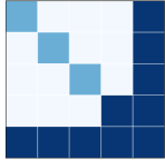
(c) $\Sigma_{lt}^{r}$

(d) $\Sigma_{lt}^{c}$

Figure 7. Structure of $\Sigma(\alpha)$ induced by sparsity of $\alpha$. Zero entries are in light blue, unit entries are in medium blue, and the unrestricted entries are in dark blue.

If the map $\alpha\mapsto\Sigma_{lt}(\alpha)$ is instead replaced by an essentially equivalent representation $\alpha\mapsto\Sigma_{ut}(\alpha)$ in terms of upper triangular matrices, the analogous structures $\Sigma_{ut}^{r}(\alpha)$ and $\Sigma_{ut}^{c}(\alpha)$ are the same as for $\Sigma_{lt}^{c}(\alpha)$ and $\Sigma_{lt}^{r}(\alpha)$ respectively.

There is a relationship between the two parametrizations $\alpha\mapsto\Sigma_{lt}(\alpha)$ and $(\alpha,d)\mapsto\Sigma_{ltu}(\alpha,d)$ if zeros in $d$ are allowed. To see this, write

$$\Sigma_{lt}=\exp(L)\exp(L^{{\rm T}})=\exp(L_{u}D_{1})\exp((L_{u}D_{1})^{{\rm T}}),$$

where $D_{1}\in\textsf{D}(p)$ and $L_{u}\in\textsf{LT}_{\textsf{u}}(p)$. On writing $L_{u}D_{1}=L_{s}+D_{1}$, where $L_{s}\in\textsf{LT}_{\textsf{s}}(p)$ and using the properties of matrix exponential,

$$\Sigma_{lt}=\exp(L)\exp(L^{{\rm T}})=\exp(L_{s})\exp(D_{1}+D_{1}^{{{\rm T}}})\exp(L_{s}^{{\rm T}}),$$

which recovers the LTU decomposition with $D=2D_{1}$. Thus if $d$ is allowed to have zeros, there is an exact relationship between the coefficients of the expansion of $\Sigma_{ltu}$ and those of $\Sigma_{lt}$.

5. Statistical interpretation in a notional Gaussian model

The basis coefficients $\alpha$ and the structures expounded in Corollaries 4.1–4.4 are directly interpretable. Those of Corollaries 4.1 and 4.2 were discussed by Battey (2017) and Rybak & Battey (2021) respectively. The more interesting structures of Corollaries 4.3 and 4.4 are elucidated here from a graphical modelling perspective, assuming for some of the latter statements an underlying Gaussian model.

5.1. Interpretation of basis coefficients

With $[p]=\{1,\ldots,p\}$, let $a\subset[p]$ and $b=[p]\backslash a$ be disjoint subsets of variable indices, and in a departure from previous notation aligning with graphical modelling convention, let $I_{aa}$ denote the identity matrix of dimension $|a|$. As a consequence of a block-diagonalization identity for symmetric matrices (Cox & Wermuth, 1993; Wermuth & Cox, 2004),

$$\Sigma=\begin{pmatrix}\Sigma_{aa}&\Sigma_{ab}\\ \Sigma_{ba}&\Sigma_{bb}\end{pmatrix}=\begin{pmatrix}I_{aa}&0\\ \Sigma_{ba}\Sigma_{aa}^{-1}&I_{bb}\end{pmatrix}\begin{pmatrix}\Sigma_{aa}&0\\ 0&\Sigma_{bb.a}\end{pmatrix}\begin{pmatrix}I_{aa}&\Sigma_{aa}^{-1}\Sigma_{ab}\\ 0&I_{bb}\end{pmatrix}.$$ (5.1)

The matrix identity (5.1) holds independently of any distributional assumptions on the underlying random variables. The components $\Pi_{b|a}:=\Sigma_{ba}\Sigma_{aa}^{-1}\in\mathbb{R}^{|b|\times|a|}$, $\Sigma_{aa}\in\textsf{PD}(|a|)$ and $\Sigma_{bb.a}:=\Sigma_{bb}-\Sigma_{ba}\Sigma_{aa}^{-1}\Sigma_{ab}\in\textsf{PD}(|b|)$ are the so-called partial Iwasawa coordinates for $\textsf{PD}(p)$ based on a two-component partition $|a|+|b|=p$ of $p$ (Terras, 1988, Chapter 4). For a statistical interpretation, let $Y=(Y_{a}^{{\rm T}},Y_{b}^{{\rm T}})^{{\rm T}}$ be a mean-centred random vector with covariance matrix $\Sigma$, $\Pi_{b|a}$ is the matrix of regression coefficients of $Y_{a}$ in a linear regression of $Y_{b}$ on $Y_{a}$ and $\Sigma_{bb.a}$ is the residual covariance matrix, i.e. $Y_{b}=\Pi_{b|a}Y_{a}+\varepsilon_{b}$ and $\Sigma_{bb.a}=\text{var}(\varepsilon_{b})$. More explicitly, on fixing a component $i\in b$ and $j\in a$, the corresponding component of $\Pi_{b|a}$ is

$$\beta_{i.ja}=\frac{\partial\mathbb{E}\{(Y_{i}\mid Y_{a\backslash j}=y_{a\backslash j})(y_{j})\}}{\partial y_{j}}.$$ (5.2)

The conditional expectation indicates conditioning on observed values of $Y_{a\backslash j}$ with $y_{j}$ as a free variable. Although the ordering in Corollary 4.4 is immaterial, it is notationally convenient to order the underlying random variables as $Y=(Y_{1},\ldots,Y_{p})^{{\rm T}}$ and apply the block-diagonalization identity recursively with, say $a(1)=1$, $b(1)=[p]\backslash a(1)$, $a(k)=k$, $b(k)=b(k-1)\backslash a(k)$. There results a block diagonalization in $1\times 1$ blocks, recovering the LDU decomposition. In this representation, the $ii$th entry of $\Psi=e^{D}$ from Corollary 4.4 is given by $\Sigma_{ii.[i-1]}$, a mean-squared error from the linear projection of $Y_{i}$ on $Y_{1},\ldots,Y_{i-1}$, and the $ij$th entry of the lower-triangular matrix $U$, for $j<i$, is given by $U_{ij}=\beta_{i.j[j]}$, that is, the coefficient of $Y_{j}$ in a regression of $Y_{i}$ on $Y_{1},\ldots,Y_{j}$.

Further interpretation for the entries of $U$ is obtained by considering an upper-triangular decomposition of the precision matrix. For an arbitrary partition $Y=(Y_{a}^{{{\rm T}}},Y_{b}^{{{\rm T}}})^{{{\rm T}}}$, let $\Sigma^{-1}$ be partitioned accordingly as

$$\Sigma^{-1}=\begin{pmatrix}\Sigma^{aa}&\Sigma^{ab}\\ \Sigma^{ba}&\Sigma^{bb}\end{pmatrix}.$$

The block upper-triangular decomposition takes the form,

$$\Sigma^{-1}=\Upsilon\Gamma\Upsilon^{{{\rm T}}}=\begin{pmatrix}I_{aa}&\Sigma^{ab}(\Sigma^{bb})^{-1}\\ 0&I_{bb}\end{pmatrix}\begin{pmatrix}\Sigma^{aa.b}&0\\ 0&\Sigma^{bb}\end{pmatrix}\begin{pmatrix}I_{aa}&0\\ (\Sigma^{bb})^{-1}\Sigma^{ba}&I_{bb}\end{pmatrix},$$

where $\Sigma^{aa.b}=\Sigma^{aa}-\Sigma^{ab}(\Sigma^{bb})^{-1}\Sigma^{ba}$. Then,

$$U^{-1}=\Upsilon^{{{\rm T}}}=\begin{pmatrix}I_{aa}&0\\ (\Sigma^{bb})^{-1}\Sigma^{ba}&I_{bb}\end{pmatrix}^{-1}.$$

An alternative expression for the matrix of regression coefficients of $Y_{b}$ in a regression of $Y_{b}$ on $Y_{a}$ is thus $\Pi_{b|a}=-(\Sigma^{bb})^{-1}\Sigma^{ba}$ (Wermuth & Cox, 2004), which corresponds to the non-zero off-diagonal block of $U^{-1}$.

By partitioning $\Sigma^{-1}$ recursively until $\Upsilon$ is upper-triangular, we obtain that the $i$th row of $U^{-1}$ contains minus the regression coefficients of $Y_{i}$ on $Y_{1},\ldots,Y_{i-1}$. Let $\tilde{U}=\Upsilon^{{{\rm T}}}-I$, where $\tilde{U}$ is a strictly lower-triangular matrix, and let $\bar{U}=-\tilde{U}$. In particular, $\bar{U}_{ij}=\beta_{i.j[i-1]}$ for $j<i$, namely, the coefficient of $Y_{j}$ in a regression of $Y_{i}$ on $Y_{1},\ldots,Y_{i-1}$. Then,

$$U=(I+\tilde{U})^{-1}=I+\sum_{j=1}^{p-1}(-1)^{j}\tilde{U}^{j}=I+\sum_{j=1}^{p-1}\bar{U}^{j},$$

where we used that, for a nilpotent matrix $N$ of degree $k$, $(I+N)^{-1}=I+\sum_{j=1}^{k-1}(-1)^{j}N^{j}$.

For a set of three variables $(Y_{1},Y_{2},Y_{3})$, the marginal effect of $Y_{3}$ on $Y_{1}$ is related to the conditional effects through Cochran’s recursion (Cochran,, 1938),

$$\beta_{3.1}=\beta_{3.12}+\beta_{3.21}\beta_{2.1},$$ (5.3)

which generalizes to an arbitrary number of variables in the manner indicated below. The right-hand side of equation (5.3) corresponds to tracing the effects of $Y_{3}$ on $Y_{1}$ along two paths connecting the nodes in a notional recursive system of random variables $(Y_{1},Y_{2},Y_{3})$, with edge weights set equal to the corresponding regression coefficients. A directed edge in a recursive system can exist from node $j$ to node $i$ only if $j<i$. Thus, there are two possible paths from $Y_{1}$ to $Y_{3}$, namely $Y_{1}\rightarrow Y_{3}$ and $Y_{1}\rightarrow Y_{2}\rightarrow Y_{3}$, which correspond to the first and second term in (5.3) respectively.

The lower-triangular matrices $U$ and $\bar{U}$ have the form,

$$\bar{U}=\begin{pmatrix}0&0&0\\ \beta_{2.1}&0&0\\ \beta_{3.12}&\beta_{3.21}&0\end{pmatrix},\quad U=I+\bar{U}+\bar{U}^{2}=\begin{pmatrix}1&0&0\\ \beta_{2.1}&1&0\\ \beta_{3.12}+\beta_{3.21}\beta_{2.1}&\beta_{3.21}&1\end{pmatrix}$$ (5.4)

The entry $U_{ij}$ for $j<i$ thus corresponds to the sum of effects of $Y_{j}$ on $Y_{i}$ along all paths connecting the two nodes. When the joint distribution of $(Y_{1},Y_{2},Y_{3})$ is Gaussian, linear regression coefficients correspond to conditional dependencies, and the trivariate system can be represented by a directed acyclic graph, as shown in Figure 8(A).

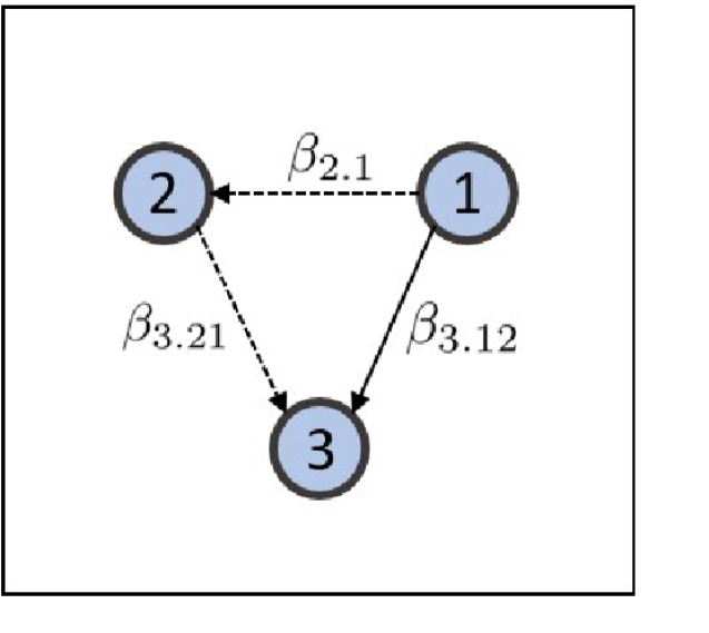
(a)

(b)

Figure 8. Directed acyclic graphs with edge weights given by regression coefficients $\beta$.

For a system of four variables, $(Y_{1},Y_{2},Y_{3},Y_{4})$ with a corresponding directed acyclic graph of the form shown in Figure 8(B), we have,

$$U=\begin{pmatrix}1&0&0&0\\ \beta_{2.1}&1&0&0\\ \beta_{3.12}+\beta_{3.21}\beta_{2.1}&\beta_{3.21}&1&0\\ \beta_{4.123}+\beta_{4.321}\beta_{3.21}\beta_{2.1}+\beta_{4.321}\beta_{3.12}&\beta_{4.213}+\beta_{4.321}\beta_{3.21}&\beta_{4.321}&1\end{pmatrix}.$$ (5.5)

Again, $U_{ij}$ for $j<i$ corresponds to the sum of effects of $Y_{j}$ on $Y_{i}$ along all directed paths connecting the two nodes, with edge weights given by regression coefficients, i.e. the marginal effect of $Y_{j}$ on $Y_{i}$ via Cochran’s recursion.

Using the properties of matrix logarithm,

$$L=\log(U)=\log[(I+\tilde{U})^{-1}]=-\log(I+\tilde{U})=\sum_{k=1}^{p-1}\frac{(-1)^{k}\tilde{U}^{k}}{k}=\sum_{k=1}^{p-1}\frac{\bar{U}^{k}}{k}.$$

Thus, the element $(i,j)$ of $L=\log(U)$, and, by extension, the corresponding coefficient in the basis expansion of $L$, is equal to the weighted sum of effects of $Y_{j}$ on $Y_{i}$ along all paths connecting the two nodes, with weights inversely proportional to the length of a given path. Estrada & Higham, (2010) and Kloster & Gleich, (2014) present some applications in which shorter paths are more important than longer ones, leading to length-based weighted averages of paths between nodes.

5.2. Interpretation of sparsity structures

Using the natural ordering in equation (5.2), the entries of $U$ encapsulate dependencies between each pair of variables, $Y_{j}$, $Y_{i}$, $j<i$, conditional on other variables among $Y_{1},\ldots,Y_{j-1}$, and marginalizing over the remaining variables $Y_{j+1},\ldots Y_{i-1},Y_{i+1},\ldots Y_{p}$.

In the terminology of e.g. Cox & Wermuth (1996), marginalization over a variable $k$ indicated by $\sslash\circ$ in the depiction below, induces an edge between $i$ and $j$ if the marginalized variable is a transition node or a source node in a parent graph. No direction in the induced edge is implied if the marginalized variable is a source node, which is indicated by ----.

$$i\longleftarrow\sslash\circ\longrightarrow j, i\longleftarrow\sslash\circ\longleftarrow j,$$

$$i\;\text{-}\text{-}\text{-}\text{-}\;j,\quad\;\; \quad\;i\longleftarrow j.$$

By contrast, if $i$ and $j$ are separated by a sink node in $a$, then conditioning on such a variable, indicated by $\square$$\circ$ below, is edge inducing, with no direction implied.

$$i\longrightarrow\text{\raisebox{-1.13809pt}{$\square$}}\circ\longleftarrow j,$$

$$i\;\text{---}\;j.$$

The entry $U_{ij}$ for $j<i$ is zero if the effects of $Y_{j}$ on $Y_{i}$ cancel out. This happens, for example, when $\beta_{3.12}=-\beta_{3.21}\beta_{2.1}$ in equation (5.3). Alternatively, when no cancellations are present, $U_{ij}=0$, $i>j$, implies an absence of a directed path from $j$ to $i$ in the notional directed acyclic graph. In addition, nodes $1\ldots j-1$ cannot be sink nodes, and nodes $j+1,\ldots,i-1,i+1,\ldots,p$ cannot be transition or source nodes.

An assumption that $Y$ is Gaussian of mean zero and covariance $\Sigma$ allows the zeros in $U$ to be interpreted as conditional independencies. If the $i$th row of $\Theta=U-I_{p}$ consists entirely of zeros, the dependence between $i$ and any $j<i$ can be explained away by conditioning on the remaining variables $\{1,\ldots,(j-1)\}$. This can happen for all $j<i$ only if $i\perp\!\!\!\perp j$ for all $j<i$, i.e., there are no direct edges between $i$ and $j<i$, and the only connecting nodes, if any, are sink nodes $k>i$.

$$i\longrightarrow k\longleftarrow j,\quad\quad j<i<k.$$

Suppose that $U-I_{p}$ from Corollary 4.4 has a zero $j$th column. This implies that for every $i>j$, the only source or transition nodes connecting $i$ and $j$ are in the conditioning sets $\{1,\ldots,j-1\}$ (otherwise dependence is induced through marginalization), and that there are no sink nodes among these conditioning variables (as conditioning on sink-nodes is edge-inducing). Consequently, the examples from Figure 7 can be represented by directed acyclic graphs presented in Figure 9.

(a) $\Sigma_{lt}^{r}(\alpha)$

(b) $\Sigma_{lt}^{c}(\alpha)$

Figure 9. Directed acyclic graphs corresponding to an example depicted in Figure 7. Arrows indicate directed edges and nodes correspond to random variables.

More generally, suppose that a random vector $Y$ is partitioned into four blocks of variables $Y=(Y_{1}^{{\rm T}},Y_{2}^{{\rm T}},Y_{3}^{{\rm T}},Y_{4}^{{\rm T}})^{{\rm T}}$ and that the lower-triangular matrix $\Theta$ in the statements of corollaries 4.3 and 4.4 has zero columns corresponding to $Y_{2}$ and zero rows corresponding to $Y_{3}$, that is, $Y_{2}$ is of dimension $d_{c}^{*}$ and $Y_{3}$ is of a dimension $d_{r}^{*}$. The directed acyclic graph of the random vector $Y$ is presented in Figure 10. Each square corresponds to a group of random variables/nodes. No connections are present among groups of variables represented by white squares, while arbitrary connections can be present within groups represented by white squares. A directed edge between groups of variables denotes a directed edge between each pair of nodes in the two groups. Double-headed arrow indicates that either of the directions can be present.

Figure 10. Directed acyclic graph corresponding to transformations $\Sigma_{lt}(\alpha)$ and $\Sigma_{ltu}(\alpha)$ for a random vector $Y$ partitioned into four subvectors $Y=(Y_{1}^{{\rm T}},Y_{2}^{{\rm T}},Y_{3}^{{\rm T}},Y_{4}^{{\rm T}})^{{\rm T}}$. The lower-triangular matrix $\Theta$ in corollaries 4.3 and 4.4 has zero columns corresponding to random variables in $Y_{2}$ and zero rows corresponding to variables in $Y_{3}$. See main text for an explanation of arrows and shading.

6. Geometric insight

Our approach of §3 can be intuited geometrically through the action of a positive definite matrix $S\in\textsf{PD}(p)$: the condition $\langle Sx,x\rangle>0$ for every $x\in\mathbb{R}^{p}$ implies that the angle between a vector $x$ and $Sx$ is smaller than $\pi/2$, and they both lie on the same side of the hyperplane to which $x$ is perpendicular; alternatively, in the coordinate system given by the orthogonal eigenvectors of $S$, the vector $Sx$ is merely stretched along the same direction by a positive factor determined by the eigenvalues of $S$. The same-sidedness of the action of $S$ can thus be decomposed into rotations that preserve orientations (i.e., $\textsf{SO}(p)$), restricted shearing (i.e., $\textsf{LT}_{\textsf{u}}(p)$), and scaling (i.e., $\textsf{D}_{+}(p)$).

The parameter domains $N$ considered in §3 are subsets of $\mathbb{R}^{p(p+1)/2}$ that correspond to infinitesimal versions of such transformations. For example, elements of $\textsf{Sk}(p)$ are infinitesimal rotations in $\mathbb{R}^{p}$ in the following sense: for every curve $\gamma:[0,1]\to\textsf{SO}(p)$ with $\gamma(0)=I$ we have $\frac{d}{dt}\gamma(t)|_{t=0}=A$ for some $A\in\textsf{Sk}(p)$ such that $I+tA$ is approximately a rotation for small $t$. In similar fashion, elements of $\textsf{D}(p)$ and $\textsf{LT}_{\textsf{s}}(p)$ are infinitesimal scale and shear transformations in $\mathbb{R}^{p}$, respectively. The vector space structure of the Lie algebras allows us to combine infinitesimal rotation, scale and shear transformations via vector addition and scale operations, which then allows us to quantify and interpret sparsity in the ensuing positive definite matrix. Thus each parametrization of $\textsf{PD}(p)$ uses as coordinates for the domain $N$ a combination of geometrically interpretable transformations, which when put together constitutes a positive definite transformation. Section 4 details the structure of subsets of $\textsf{PD}(p)$ to which sparse subsets of $N$ map.

The geometric interpretation of sparsity in $(\alpha,d)$ is as a quantification of the amount of shear and scaling that the positive definite $\Sigma_{ltu}(\alpha,d)$ applies to a vector $x\in\mathbb{R}^{p}$.

The Lie group exponential map, given by the matrix exponential (see Appendix A), $\operatorname{\mathbf{expo}}:\mathfrak{g}\to G$ is surjective for $\mathfrak{g}\in\{\textsf{Sk}(p),\textsf{Sym}(p),\textsf{LT}_{\textsf{s}}(p),\textsf{LT}(p)\}$ with corresponding $G\in\{\textsf{SO}(p),\textsf{PD}(p),\textsf{LT}_{\textsf{u}}(p),\textsf{LT}_{+}(p)\}$, but not for the general linear group $\textsf{GL}(p)$, unless the (field) of entries are complex. This ensures, for example, that every rotation matrix and upper triangular matrix with positive or unit diagonal is available for constructing a positive definite matrix in the images of $\Sigma_{o},\Sigma_{lt}$ and $\Sigma_{ltu}$, respectively. With this in mind, we can interpret the sparsity level $\|\alpha\|_{0}$ as the dimension of a submanifold of $\textsf{PD}(p)$ that corresponds to a combination of scale, rotation, and shear transformation, which when put together in some proportion results in a positive definite transformation given by $\Sigma(\alpha)$.

For example, consider the map $\Sigma_{o}$ with $s_{1},s_{2}$ numbers of non-zero coefficients in $\alpha$ and $d$, respectively, with $s:=s_{1}+s_{2}$. The image of $\Sigma_{o}$ is an $s$-dimensional connected submanifold of $\textsf{PD}(p)$ comprising an $s_{1}$ dimensional submanifold of $\textsf{SO}(p)$ and $s_{2}$-dimensional submanifold of $\textsf{D}_{+}(p)$; the image of $\alpha\mapsto e^{L(\alpha)}$ need not be a subgroup of $\textsf{SO}(p)$ since the subspace spanned by the subset of $\mathcal{B}_{sk}$ corresponding to $s_{1}$ non-zero coefficients need not be a Lie subalgebra of $\textsf{Sk}(p)$; the same applies to the map $d\mapsto e^{D(d)}$. In this case, the sparsity levels $s_{1}$ and $s_{2}$ in the new domain $N$ relates to dimensions of the rotation and scaling submanifolds of $\textsf{PD}(p)$, and configuration of the $s$ non-zero coefficients relates to the choice of $s$-dimensional submanifold of $\textsf{PD}(p)$. Evidently, such geometric interpretation are available for the other reparametrization maps as well with respect to shear and scale submanifolds of $\textsf{PD}(p)$.

7. Sparsity comparisons

7.1. Exact zeros

Section 4 studied the structure induced on $\Sigma$, in terms of exact zeros, through sparsity of $\alpha$. An aspect not discussed in detail there is the observation of Battey (2017) and Rybak & Battey (2021) that $\alpha$ may be considerably sparser than $\sigma=\operatorname{\mathbf{vech}}(\Sigma(\alpha))$, both in terms of exact zeros and approximate zeros. This is most clearly illustrated through the parametrization $\alpha\mapsto\Sigma_{pd}(\alpha)$. As shown by Battey (2017) and as is implicit in Corollary 4.1, the number of non-unit eigenvalues of $\Sigma_{pd}(\alpha)$ when $\|\alpha\|_{0}=s^{*}<p$ is $d^{*}<2s^{*}$ and the number non-zero entries of any eigenvector $\xi_{j}$ associated with a non-unit eigenvalue $\lambda_{j}$ of $\Sigma$ is also $d^{*}$. Thus, with $\mathcal{A}=\{j:\lambda_{j}\neq 1\}$, the $(q,r)$th entry of the matrix logarithm is $L_{qr}=\sum_{j\in\mathcal{A}}\log(\lambda_{j})\xi_{qj}\xi_{rj}$. If $q\in\mathcal{A}$, then $\xi_{qj}\neq 0$ and $\log(\lambda_{j})\neq 0$ for $j\in\mathcal{A}$. However $L_{qr}=0$ is still feasible by cancellation in the sum even if $q,r\in\mathcal{A}$. Suppose that $L_{qr}=0$. If $q\in\mathcal{A}^{c}$ or $r\in\mathcal{A}^{c}$ then $\Sigma_{qr}=0$ by Corollary 4.1. However if $L_{qr}=0$ and $q,r\in\mathcal{A}$, then $\Sigma_{qr}\neq 0$ by construction, illustrating the possibility that $L=\log(\Sigma)$ may be substantially sparser than $\Sigma$. A random sparse $L$ is necessarily sparser in terms of exact zeros than $e^{L}$. However a random dense $\Sigma$ with the structure specified by Corollary 4.1 almost surely has a matrix logarithm with the same degree of sparsity in terms of exact zeros as $\Sigma$. Notwithstanding, it is often the case that $L$ is much sparser than $\Sigma$ under more general notions of sparsity. A similar phenomenon applies in the other parametrizations. The relative sparsity levels in the four parametrizations are explored in §7.2.

7.2. Approximate zeros

A more general notion of sparsity suitable for the four cases is $q$-sparsity. Defined for $\alpha\mapsto\Sigma_{pd}(\alpha)$ and $\alpha\mapsto\Sigma_{lt}(\alpha)$ as

$$s_{q}^{*}=s_{q}^{*}(\alpha)=\Bigl{(}\textstyle{\sum_{j=1}^{p(p+1)/2}|\alpha_{j}|^{q}}\Bigr{)}^{1/q}$$

and for $(\alpha,d)\mapsto\Sigma_{o}(\alpha,d)$ and $(\alpha,d)\mapsto\Sigma_{ltu}(\alpha,d)$ as

$$s_{q}^{*}=s_{q}^{*}(\alpha,d)=\Bigl{(}\textstyle{\sum_{j=1}^{p(p-1)/2}|\alpha_{j}|^{q}}+\textstyle{\sum_{j=1}^{p}|d_{j}|^{q}}\Bigr{)}^{1/q}.$$

A comparable definition of $q$-sparsity for $\Sigma\in\textsf{PD}(p)$ is

$$s_{q}=s_{q}(\sigma)=\Bigl{(}\textstyle{\sum_{j=1}^{p(p+1)/2}}|\sigma_{j}|^{q}\Bigr{)}^{1/q}.$$

In the simulations to follow, sparsity after reparametrization is compared to sparsity on the original scale via the ratio, $s_{q}^{*}/s_{q}$.

We consider both directions of the discussion in §7.1 by simulation for $q>0$. With $\textsf{V}(p)$ as one of the constituent Lie subalgebras in the Iwasawa decomposition (2.1), in one direction, we generate a sparse $L\in\textsf{V}(p)$ or $(L,D)\in\textsf{V}(p)\otimes\textsf{D}(p)$ and compare their $q$-sparsity level to that of the corresponding covariance matrix $\Sigma\in\textsf{PD}(p)$. For the converse question, we generate a dense $\Sigma\in\textsf{PD}(p)$ and compare its $q$-sparsity level to that of $L\in\textsf{V}(p)$ or $(L,D)\in\textsf{V}(p)\otimes\textsf{D}(p)$ after reparametrization.

7.2.1. Simulations for sparse $L\in\textsf{V}(p)$

Figure 11 was obtained by generating 250 realizations of a random, sparse $L\in\textsf{V}(p)$ with $p=20$ by taking the support of $\alpha$ to be random samples of size $s^{*}$ from the index set $\{1,\ldots,p(p-1)/2\}$ for $L\in\textsf{Sk}(p)$ and $L\in\textsf{LT}_{\textsf{s}}$ or from the index set $\{1,\ldots,p(p+1)/2\}$ for $L\in\textsf{Sym}(p)$ and $L\in\textsf{LT}$. This was done for different values of $s^{*}$ as indicated in Figure 1. The values of the nonzero basis coefficients were then drawn from a uniform distribution on $[-1,1]$. The positive elements of the diagonal matrices in the decompositions $\Sigma_{o}=O\Lambda O^{{\rm T}}$ and $\Sigma_{ltu}=U\Psi U^{{\rm T}}$ are obtained from $\chi^{2}_{4}$ and $\exp(1)$ distributions, as indicated.

$\Sigma_{pd}$                                                      $\Sigma_{lt}$

$\Sigma_{o}$, $\chi^{2}_{4}$                                               $\Sigma_{o}$, $\exp(1)$

$\Sigma_{ltu}$, $\chi^{2}_{4}$                                             $\Sigma_{ltu}$, $\exp(1)$

Figure 11. Simulations for random sparse $L\in\textsf{V}(p)$. Simulated ratios $s_{q}^{*}/s_{q}$ for different values of $s^{*}=\|\alpha\|_{0}$ and $q$.

7.2.2. Simulations for dense $\Sigma\in\textsf{PD}(p)$

Rather than constructing $\Sigma$ from a sparse $L\in\textsf{V}(p)$, we now sample covariance matrices directly, and construct the corresponding tranformation on the logarithmic scale. A random dense $\Sigma$ is obtained from the representation $\Sigma=O\Lambda O^{T}$ by generating $O$ uniformly over $\textsf{SO}(p)$ according to Haar measure and by generating the positive of the diagonal matrix $\Lambda$ from a gamma distribution of shape $\tau$ and scale $\kappa$, written $\Gamma(\tau,\kappa)$. The results are reported in Figure 12.

(a) $\Sigma_{pd}$

(b) $\Sigma_{o}$

(c) $\Sigma_{lt}$

(d) $\Sigma_{ltu}$

Figure 12. Simulations for random dense $\Sigma\in\textsf{PD}(p)$. Simulated averages (standard deviations) of the ratio $s_{q}^{*}/s_{q}$ for different values of $q$ and different distributions of eigenvalues of $\Sigma$. Blue entries signify greater sparsity after reparametrization.

8. Discussion and open problems

8.1. Methodological implications: some provisional remarks

As emphasized throughout, the focus of this work is on elucidating population-level structure, thereby pointing to an interpretation of sparsity after reparametrization and also facilitating the assessment of assumptions. In particular, a key aspect is whether sparsity assumptions, required to prevent the accumulation of estimation error and thereby provide statistical guarantees for many multivariate procedures of interest, are likely to be in reasonable accord with reality.

From a methodological point of view, two broad approaches are to assume a plausible set of graphical structures, leading to a reparametrization in which the subsumed structure is sparse, or to seek to deduce the sparsest representation empirically.

There are numerous open challenges associated with these two broad possibilities, which we do not take up here. Perhaps primary among these is the existence and uniqueness of the constrained maximum likelihood estimator under the relevant constraints, analogous to the discussion of Zwiernik et al. (2017) for Gaussian models with linear constraints on the covariance matrix. Zwiernik (2023) has highlighted further difficulties in using the log-likelihood function to estimate a covariance matrix when there are linear restrictions on its matrix logarithm, and proposed to instead use the Bregman divergence as a loss function. Open questions are whether his analysis extends to the other parametrizations considered here, and whether model adequacy can be assessed. A further set of methodological questions emerges once consideration is given to which sparsity constraints should be allowed for $\alpha$, i.e. whether each coefficient should be treated on an equal footing, or whether preference should be given to configurations that generate the most interesting structures according to e.g. Corollary 4.4 and the discussion of §5.

Since the matrix logarithms in each of the four parametrizations of §3 belong to different spaces, there are difficulties in traversing reparametrization space to find the most convenient representation empirically. One conceivable resolution is based on the observation that all four sparse parametrizations are representable in terms of a strictly lower triangular matrix $L_{s}\in\textsf{LT}_{\textsf{s}}(p)$ and a diagonal matrix $D\in\textsf{D}(p)$. With $\mathcal{B}_{ltu}$ the canonical basis for $\textsf{LT}_{\textsf{s}}(p)$ described in §3.6, and with $\mathcal{B}_{diag}=\{D_{1},\ldots,D_{p}\}$ the canonical basis for $\textsf{D}(p)$ with elements $D_{j}=e_{j}e_{j}^{{\rm T}}$, the four cases of interest can be represented in terms of a common basis on noting that

$$L = L_{s}+L_{s}^{{\rm T}}+D,\quad L\in\textsf{Sym}(p),\hskip 4.55254ptL_{s}\in\textsf{LT}_{\textsf{s}}(p),\;\;D\in\textsf{D}(p),$$

$$L = L_{s}-L_{s}^{{\rm T}},\hskip 29.87547ptL\in\textsf{Sk}(p),\hskip 12.80365ptL_{s}\in\textsf{LT}_{\textsf{s}}(p),$$

$$L = L_{s}+D,\hskip 34.14322ptL\in\textsf{LT}(p),\hskip 10.81218ptL_{s}\in\textsf{LT}_{\textsf{s}}(p),\;\;D\in\textsf{D}(p),$$

$$L = L_{s},\hskip 54.06006ptL\in\textsf{LT}_{\textsf{s}}(p),\hskip 8.5359ptL_{s}\in\textsf{LT}_{\textsf{s}}(p).$$

where $L_{s}\in\textsf{LT}_{\textsf{s}}(p)$ and $D\in\textsf{D}(p)$ have basis expansions in $\mathcal{B}_{ltu}$ and $\mathcal{B}_{diag}$. In principle, this provides a means of parametrizing a ‘path’ (actually a hypersurface) through parametrization space by writing

$$Q(\theta)=L_{s}(\alpha)+\text{sgn}(\delta)L_{s}^{{\rm T}}(\alpha)+(1-\gamma)D(\beta),\quad\delta\in\mathbb{R},\;\gamma\in[0,1],$$

where $\theta=(\alpha,\beta,\gamma,\delta)$, and

$$(\theta,\varepsilon)\mapsto\Sigma(\theta,\varepsilon)=(e^{Q(\theta)})(e^{D(\beta)})^{\gamma\text{sgn}(\varepsilon)}((e^{Q(\theta)})^{{\rm T}})^{\text{sgn}(\varepsilon)},\;\varepsilon\in\mathbb{R}$$ (8.1)

This hypersurface through model space, while parametrized, is not a parametrization in the formal sense discussed in Appendix B, as the presence of the sign function $\text{sgn}(\cdot)$ violates injectivity. Both sign functions can be dropped at the expense of the positive definiteness of $\Sigma(\theta,\varepsilon)$. This is similar in spirit to the encompassing model formulation for regression transformation of Box & Cox (1964), who required a single parameter to traverse outcome-transformation space, and thereby model space. Similarly to the representation above, only certain values of the transformation parameter give reasonable models, as discussed by Box & Cox (1982).

8.2. Further exploration of the partial Iwasawa decomposition

In equation (5.1), the matrix

$$U_{b|a}:=\begin{pmatrix}I_{aa}&0\\ \Sigma_{ba}\Sigma_{aa}^{-1}&I_{bb}\end{pmatrix}$$

belongs to a restricted subset of $\textsf{LT}_{\textsf{u}}(p)$ and the matrix

$$D_{b|a}:=\begin{pmatrix}\Sigma_{aa}&0\\ 0&\Sigma_{bb.a}\end{pmatrix}$$

is block diagonal with positive definite blocks. This suggests a version of the $\Sigma_{ltu}$ parametrization in which sparsity is imposed on $\log(U_{b|a})$ and on the blocks of $D_{b|a}$ after reparametrization. This is likely to induce a range of further structures on the original domain, with corresponding graphical interpretation.

Conversely, for every positive definite $\Sigma\in\textsf{PD}(p)$ there exists a unique triple $V\in\textsf{PD}(r),W\in\textsf{PD}(s)$ and $H\in\mathbb{R}^{r\times s}$ (Terras, 1988, Chapter 4) such that

$$\Sigma=\begin{pmatrix}I&H\\ 0&I\end{pmatrix}\begin{pmatrix}V&0\\ 0&W\end{pmatrix}\begin{pmatrix}I&0\\ H^{{\rm T}}&I\end{pmatrix},$$

the partial Iwasawa decomposition, and hence the $\Sigma_{ltu}$ parametrization with the two-block structure corresponding to the partition $p=r+s$ of $p$, can conceivably be used to parametrize several other statistically interesting graphical models with appropriate restrictions on $V,W$ and $H$. Indeed, this can be further generalized to any partition $r_{1}+\cdots+r_{k}=p$ of $p$ with $k\leq p$, which then offers additional possibilities.

Interestingly, information geometry of the zero-mean multivariate Gaussian (Skovgaard, 1984) induced by the Fisher Information metric tensor coincides with the quotient geometry of $\textsf{PD}(p)\cong\textsf{GL}(p)/\textsf{O}(p)$ under a Riemannian metric that is invariant to the transitive action of $\textsf{GL}(p)$. Upon representing a positive definite covariance matrix $\Sigma$ in the partial Iwasawa coordinates $(\Sigma_{aa},\Sigma_{ba}\Sigma_{aa}^{-1},\Sigma_{bb.a})$, the metric is endowed with an interpretation compatible with a suitable graphical model and a corresponding $\Sigma_{ltu}$ parametrization. We will develop this connection elsewhere.

Appendix A Matrix groups

We restrict attention to only those concepts from group theory that bear direct relevance to the exposition and proofs. An excellent source of reference for matrix groups is Baker (2001). The action of a group $G$ on a set $X$ is a continuous map $X\times G\to X,(g,x)\to gx$. The orbit $[x]$ of $x\in X$ is the equivalence class $\{gx:g\in G\}$, and the set of orbits $X/G:=\{[x]:x\in X\}$ is a partition of $X$ known as the quotient of $X$ under the action of $G$. A group action is said to be transitive if between any pair $x_{1},x_{2}\in X$ there exists a $g\in G$ such that $x_{2}=gx_{1}$; in other words, orbits of all $x\in X$ coincide. The subset $G_{x}=\{g\in G:gx=x\}$ of $G$ that fixes $x$ is known as the isotropy group of $x$ and if $G_{x}$ equals the identity element for every $x$, the group action is said to be free.

For every subgroup $H\subset G$ we can consider the (right) coset, or the quotient, $G/H=\{Hg:g\in G\}$ consisting of equivalence classes of $g$, where $\tilde{g}\sim g$ if $h\tilde{g}=g$ for some $h\in H$. For groups $G$ that act transitively on $X$, the map $X\to G/G_{0}$ is a bijection, where $G_{0}$ is the isotropy group of the identity element.

A group $G$ that is also a differential manifold is a Lie group. Lie groups thus enjoy a rich structure given by both algebraic and geometric operations. The tangent space at the identity element, denoted by $\mathfrak{g}$, has a special role in that, together with the group operation, it generates the entire group, i.e. every element $g\in G$ can be accessed through elements of $\mathfrak{g}$ and the group operation. It is referred to as the Lie algebra and is a vector subspace of the same dimension as the group. Relevant to the matrices introduced in §2.1, we have:

1. If $G=\textsf{GL}(p)$ with matrix multiplication as the group action, then $\mathfrak{g}=\textsf{M}(p)$.

2. If $G=\textsf{O}(p)$ or $\textsf{SO}(p)$ with matrix multiplication as the group action, then $\mathfrak{g}=\textsf{Sk}(p)$, the set of skew-symmetric matrices.

3. If $G=\textsf{LT}_{+}(p)$ with matrix multiplication as the group action, then $\mathfrak{g}$ is the set $\textsf{LT}(p)$ of lower triangular matrices.

4. If $G=\textsf{LT}_{\textsf{u}}(p)$ with matrix multiplication as the group action, then $\mathfrak{g}$ is the set $\textsf{LT}_{\textsf{s}}(p)$ of lower triangular matrices with zeros along the diagonal.

5. If $G=\textsf{PD}(p)$ with logarithmic addition as the group action (Arsigny et al., 2017) then $\mathfrak{g}=\textsf{Sym}(p)$.

When $G$ is a matrix Lie group, the usual matrix exponential can be related to the map $\operatorname{\mathbf{expo}}:\mathfrak{g}\to G$ such that $\operatorname{\mathbf{expo}}(A)=e^{A}$. Properties of $\operatorname{\mathbf{expo}}$ (e.g., injectivity) will depend on that of the matrix exponential, and hence on the topology of $G$. If $G$ is compact and connected then $e$ is surjective. If it is injective in a small neighbourhood around the origin in $\mathfrak{g}$, then it bijective. Since $G$ is also a differentiable manifold, a geometric characterisation of the matrix exponential $e$ is that it will coincide with the Riemannian exponential map under a bi-invariant Riemannian metric on $G$.

Appendix B Parametrizations of $\textsf{PD}(p)$

B.1. Proof of Proposition 3.1

Proof.

The set $\textsf{PD}(p)$ is a symmetric space of dimension $p(p+1)/2$ of noncompact type and can thus has nonpositive (sectional) curvature when equipped with a Riemannian structure (Helgason, 2001). The map $\operatorname{\mathbf{vech}}^{-1}:\textsf{Cone}_{p}\to\textsf{PD}(p)$ is injective, and we can thus pullback the metric from $\textsf{PD}(p)$ to $\textsf{Cone}_{p}$ making it non-positively curved. The set $\textsf{Cone}_{p}$, by virtue of being the interior of the convex cone $\{S\in\textsf{Sym}(p):x^{{\rm T}}Sx\geq 0,x\in\mathbb{R}^{p}\}$ of positive semidefinite matrices, is simply connected and complete. By the Cartan-Hadamard theorem (Helgason, 2001) it is thus diffeomorphic to $\mathbb{R}^{p(p+1)/2}$. ∎

B.2. Proof of Proposition 3.4

Proof.

Injectivity of $\Sigma_{{pd}}$ follows from Proposition 3.3. It is well-known that the Cholesky and LDU decompositions as used in the definitions of $\Sigma_{lt}$ and $\Sigma_{ltu}$ respectively are unique (Golub & Van Loan, 2013). Uniqueness of the LDU decomposition also stems from uniqueness of the Iwasawa decomposition of $\textsf{GL}(p)$ (Terras, 1988) through the identification $\textsf{PD}(p)\cong\textsf{GL}(p)/\textsf{O}(p)$. The maps $L(\alpha)\mapsto e^{L(\alpha)}(e^{L(\alpha)})^{{\rm T}}$ and $(L(\alpha),D(d))\mapsto e^{L(\alpha),D(d)}e^{D(d)}(e^{L(\alpha)})^{{\rm T}}$ are thus injective. When combined with injectivity of the exponential map $e:\textsf{LT}_{\textsf{s}}\to\textsf{LT}_{\textsf{u}}$ from Proposition 3.4, the parameterisation $\Sigma_{ltu}$ is injective.

The situation concerning uniqueness of the eigen decomposition $\Sigma=O\Lambda O^{{\rm T}}$ is involved, even after restriction to a subset of $\textsf{Sk}(p)$ that renders the exponential $e:\textsf{Sk}(p)\to\textsf{SO}(p)$ injective. First note that $O\in\textsf{SO}(p)$ under our parameterisation using the exponential map. Then, observe that $ORR^{{\rm T}}\Lambda RR^{{\rm T}}O^{{{\rm T}}}=O\Lambda O^{{\rm T}}$ for any $R\in\textsf{SO}(p)$, and thus pairs $(OR,R^{{{\rm T}}}\Lambda R)$ map to the same $\Sigma$ for every $R\in\textsf{SO}(p)$ for which $R^{{{\rm T}}}\Lambda R=\Lambda$, since $OR\in\textsf{SO}(p)$. Indeed, $\{R\in\textsf{SO}(p):R^{{{\rm T}}}\Lambda R=\Lambda\}$ fixes $\Lambda$ and is the isotropy subgroup $\textsf{SO}(p)_{\Lambda}$ in $\textsf{SO}(p)$ (see Appendix A). In addition to $\textsf{SO}(p)_{\Lambda}$, another source of indeterminacy comes from permutations $OP$ and $P\Lambda P^{{{\rm T}}}$, with $P\in\textsf{P}(p)$ and $|P|=1$ so that $P\in\textsf{SO}(p)$. Put together, this implies that every pair $(ORP,P\Lambda P^{{{\rm T}}})$ maps to the same $\Sigma$ as long as $R\in\textsf{SO}(p)_{\Lambda}$ and $P\in\textsf{SO}(p)$.

The situation can be salvaged if the positive elements of $\Lambda$ are all distinct so that $\textsf{SO}(p)_{\Lambda}$ reduces to the set $\textsf{D}(p)\cap\textsf{SO}(p)$ of diagonal rotation matrices with $\pm 1$ entries (Grossier et al., 2021, Theorem 3.3). In this case, the map $\pi:\textsf{SO}(p)\times\textsf{D}_{+}(p)\to\textsf{PD}(p)$ is a $2^{p-1}p!$ covering map with fibers $\pi^{-1}(\Sigma)$ consisting of matrices obtained by $p!$ permutations of elements of $\Lambda$, and a similar permutation of eigenvectors of $\Sigma$, and $2^{p-1}$ matrices in the set $\textsf{D}(p)\cap\textsf{SO}(p)$ of diagonal matrices mentioned above with unit determinant, which determine signs of the eigenvectors of $\Sigma$; there are $2^{{p-1}}$ such diagonal matrices and not $2^{p}$ owing to the unit determinant constraint.

Uniqueness can be ensured upon identifying a global cross section $S_{o}\subset\textsf{SO}(p)\times\textsf{D}_{+}(p)$ that picks out one element from every fiber such that $\pi^{-1}(\Sigma)\cap S_{o}$ is a singleton for every $\Sigma\in\textsf{PD}(p)$. For example, $S_{o}$ can be defined by selecting a particular permutation $P\Lambda P^{{{\rm T}}}$ and $ORP$ of the eigenvalues and eigenvectors of $\Sigma$ (e.g., elements of $\Lambda$ arranged in a decreasing order); since $R\in\textsf{D}(p)\cap\textsf{SO}(p)$, a fixed rule for choosing signs of the eigenvectors determines a unique $R$. Then, $S_{o}$ contains pairs $(ORP^{{\rm T}},P\Lambda P^{{\rm T}})$ for a fixed permutation $P\in\textsf{SO}(p)$. The cross section $S_{o}$ is bijective with the quotient $(\textsf{SO}(p)\times\textsf{D}_{+}(p))/\sim$ under the equivalence relation $\sim$ that identifies any two pairs $(O,\Lambda)$ that map to the same $\Sigma$.

The proof for injectivity of $\Sigma_{lt}$ follows upon noting that the exponential map $e:\textsf{LT}(p)\to\textsf{LT}_{+}(p)$ is injective when restricted to the given ball within $\textsf{LT}(p)$. This completes the proof.

∎

Appendix C Proofs for Section 4

C.1. Auxiliary results

Lemma C.1 (Axler, 2015).

Let V be a real inner-product space and let $T:\textsf{V}\rightarrow\textsf{V}$ be a linear operator on V with matrix representation $M=M(T)$. The following are equivalent: (i) $M$ is normal; (ii) there exists an orthonormal basis of V with respect to which $M=O\tilde{B}O^{-1}$ where the blocks of the block-diagonal matrix $\tilde{B}$ are either $1\times 1$ or $2\times 2$ of the form

$$\begin{pmatrix}a&-b\,\\ b&\;\;a\,\end{pmatrix}=\rho\begin{pmatrix}\cos\theta&-\sin\theta\\ \sin\theta&\;\;\;\cos\theta\end{pmatrix}.$$ (C.1)

where $a,b\in\mathbb{R}$, $b>0$, $\rho>0$ and $\theta\in[0,2\pi]$. Each $1\times 1$ block $\lambda$ is an eigenvalue of $M$, and for each $2\times 2$ block (C.1), $a+bi$ and $a-bi$ are eigenvalues of $M$.

The representation C.1 in terms of polar coordinates is convenient for subsequent calculations involving the matrix logarithm.

Lemma C.2.

Let $M\in\textsf{M}(p)$ be a normal matrix. The matrix logarithm $L$, if it exists, takes the form $OBO^{-1}$, where $O\in\textsf{O}(p)$ is orthonormal and $B$ is block diagonal with blocks of the form described in Lemma C.1.

Proof.

By Lemma C.1, $M=O\tilde{B}O^{-1}$, where $O\in\textsf{O}(p)$ is orthonormal and $\tilde{B}$ is block diagonal. Let $\lambda$ be an eigenvalue of $M$. From Proposition 3.2, existence of a logarithm requires that any negative real eigenvalues have associated with them an even number of blocks. By Lemma C.1 negative eigenvalues appear in $1\times 1$ blocks, since $2\times 2$ blocks correspond to complex conjugate pairs of eigenvalues. It follows that the matrix logarithm of a normal matrix exists if and only if negative eigenvalues have even multiplicity, in which case, we can without loss of generality construct blocks of size $2\times 2$ for a negative eigenvalue $\lambda$ of the form $\tilde{B}_{\lambda}=\lambda I_{2}=-|\lambda|I_{2}$. Then $\log(\tilde{B}_{\lambda})=\log\{(|\lambda|I_{2})(-I_{2})\}$, and since $I_{2}$ and $-I_{2}$ commute, $\log(\tilde{B}_{\lambda})=\log(|\lambda|I_{2})+\log(-I_{2})$, where

$$\log(-I_{2})=\pi\begin{pmatrix}0&-1\\ 1&0\end{pmatrix}.$$

Thus

$$\log(\tilde{B}_{\lambda})=\begin{pmatrix}\log|\lambda|&-\pi\\ \pi&\log|\lambda|\end{pmatrix},$$

which is of the form in Lemma C.1. For $2\times 2$ blocks $\tilde{B}_{\mathbb{C}}$ corresponding to complex conjugate pairs of eigenvalues of $M$, a similar argument together with

$$\log\begin{pmatrix}\cos\theta&-\sin\theta\\ \sin\theta&\;\;\;\cos\theta\end{pmatrix}=\begin{pmatrix}0&-\theta\,\\ \theta&\;\;0\,\end{pmatrix}$$

shows that

$$\log(\tilde{B}_{\mathbb{C}})=\begin{pmatrix}\log\rho&-\theta\,\\ \theta&\;\;\log\rho\,\end{pmatrix}$$

which is also of the form of Lemma C.1. ∎

Lemma C.3.

Let $M=e^{L}\in\textsf{M}(p)$. Then $M$ is normal if and only if $L$ is normal.

Proof.

Suppose that $L$ is normal, that is $L^{{\rm T}}L=LL^{{\rm T}}$. By the Jordan decomposition $L=QJQ^{-1}$, normality of $L$ implies normality of $J$. The matrix exponential $M=\exp(L)=Q\exp(J)Q^{-1}$ is normal if and only if $\exp(J)^{{\rm T}}\exp(J)=\exp(J)\exp(J)^{{\rm T}}$. Two general properties of the matrix exponential are that for matrices $A,B\in\textsf{M}(p)$ such that $AB=BA$, $\exp(A)^{{\rm T}}=(\exp(A))^{{\rm T}}$ and $\exp(A)\exp(B)=\exp(A+B)$. Thus $\exp(J^{{\rm T}})\exp(J)=\exp(J+J^{{\rm T}})=\exp(J)\exp(J^{{\rm T}})$ showing that $M$ is normal. The converse statement follows by Lemmas C.1 and C.2. ∎

Lemma C.4 (Weierstrass’s M-test, e.g. Whittaker and Watson, 1965, p.49).

Let $S_{k}(A)=s_{1}(A)+\cdots+s_{k}(A)$ be a sequence of functions such that, for all $A$ within some region $\mathcal{R}(A)$, $S_{k}(A)\leq T_{k}=t_{1}+\cdots+t_{k}$, where $(t_{j})_{j\in\mathbb{N}}$ are independent of $A$ and $T_{k}$ is a positive convergent sequence. Then $S_{k}(A)$ converges to some limit, $S(A)$ say, uniformly over $\mathcal{R}(A)$.

Lemma C.5.

For $A\in\textsf{M}(p)$, define $\psi(A)=\sum_{k=0}^{\infty}A^{k}/(k+1)!$. Then for any operator norm $\|\cdot\|_{\text{op}}$, provided that $\|A\|_{\text{op}}$ is bounded, $\|\psi(A)\|_{\text{op}}\leq\|\exp(A)\|_{\text{op}}$. Additionally, $\psi(A)\in\textsf{GL}(p)$ for any $A\in\textsf{M}(p)$.

Proof.

Let $\psi_{k}(A)=\sum_{n=0}^{k}A^{n}/(n+1)!$ and let $r\geq 0$ be such that $\|A\|_{\text{op}}\leq r$. Since the operator norm is subadditive and submultiplicative

$$\|\psi_{k}(A)\|_{\text{op}}\leq\sum_{n=0}^{k}\frac{\|A^{n}\|_{\text{op}}}{(n+1)!}\leq\sum_{n=0}^{k}\frac{\|A\|_{\text{op}}^{n}}{n!}\leq\sum_{n=0}^{k}\frac{r^{n}}{n!}\rightarrow e^{r}$$

as $k\rightarrow\infty$. Lemma C.4 applies with $S_{k}(A)=\|\psi_{k}(A)\|_{\text{op}}$.

For the second statement, it suffices by the Jordan decomposition of $A$ to show that $\psi(\lambda)\neq 0$ where $\lambda\in\mathbb{C}$ is an eigenvalue of $A$. For $\lambda=0$, $\psi(\lambda)=1$ by definition, whereas for $z\in\mathbb{C}$, $z\neq 0$, $\psi(z)=(e^{z}-1)/z\neq 0$. ∎

Lemma C.6.

Consider $M=e^{L}\in\textsf{M}(p)$ where $L\in\textsf{V}(p)$, a vector space with canonical basis $\mathcal{B}$ of dimension $d$. The matrix $M$ is logarithmically sparse in the sense that $L=L(\alpha)=\alpha_{1}B_{1}+\cdots+\alpha_{d}B_{d}$, $B_{j}\in\mathcal{B}$ with $\|\alpha\|_{0}=s^{*}$ if and only if $M=P\tilde{M}P^{{\rm T}}$, where $P$ is a permutation matrix and

$$\tilde{M}=\left(\begin{array}[]{cc}O_{11}&0\\ 0&I_{q}\end{array}\right)\left(\begin{array}[]{cc}C_{11}&C_{12}\\ 0&I_{q}\end{array}\right)\left(\begin{array}[]{cc}O_{11}^{{\rm T}}&0\\ 0&I_{q}\end{array}\right),$$ (C.2)

where $q\geq p-d_{r}^{*}$ and $O_{11}\in\textsf{O}(p-q)$, $C_{11}\in\textsf{M}(p-q)$. Moreover, if $M$ is normal, $C_{11}$ is also normal and $C_{12}=0$ in (C.2).

Proof.

Suppose first that $M=e^{L}$ is logarithmically sparse. By definition, $L$ has $p-d_{r}^{*}$ zero rows. Assume without loss of generality that $L$ is in canonical form, so that the last $p-d_{r}^{*}$ rows are zero. Thus write $L$ as a partitioned matrix with blocks upper blocks $L_{1}$, $L_{2}$ of dimensions $d_{r}^{*}\times d_{r}^{*}$ and $d_{r}^{*}\times p-d_{r}^{*}$, the remaining blocks being zero. On taking the Taylor expansion of the matrix exponential,

$$e^{L}=\left(\begin{array}[]{cc}\exp(L_{1})&\sum_{k=0}^{\infty}L_{1}^{k}L_{2}/(k+1)!\\ 0&I_{p-d_{r}^{*}}\end{array}\right)$$

which is of the form given in equation (C.2) with $O_{11}=I_{d_{r}^{*}}$.

To prove the reverse direction, we need to construct $L$ such that

$$\exp(L)=\begin{pmatrix}O_{11}C_{11}O^{{{\rm T}}}_{11}&O_{11}C_{12}\\ 0&I\end{pmatrix},\quad L=\begin{pmatrix}A&B\\ 0&0\end{pmatrix},$$ (C.3)

where the number of zero rows of $L$ is greater or equal to $p-d_{r}^{*}$. Let $\Gamma_{1}=O_{11}C_{11}O_{11}^{{{\rm T}}}$ and $\Gamma_{2}=O_{11}C_{12}$. Set $A=\log(\Gamma_{1})$, which exists by assumption since eigenvalues of $\Gamma_{1}$ are eigenvalues of $\tilde{M}$. Clearly, by the Taylor series of matrix exponential,

$$\exp(L)=\begin{pmatrix}\Gamma_{1}&\sum_{k=0}^{\infty}\frac{A^{k}}{(k+1)!}B\\ 0&I\end{pmatrix}.$$

It thus remains to be shown that $\sum_{k=0}^{\infty}\frac{A^{k}}{(k+1)!}B=\Gamma_{2}$ some $d_{r}^{*}\times p-d_{r}^{*}$ matrix $B$. Let $\psi(A)=\sum_{k=0}^{\infty}\frac{A^{k}}{(k+1)!}$. By Lemma C.5, $\psi(A)$ is invertible, and we can take $B=\psi(A)^{-1}\Gamma_{2}$. Note that the matrix logarithm of $\tilde{M}$ is not unique. However, for a real eigenvalue $\lambda$ of $\tilde{M}$, logarithm of the Jordan block $J_{k}(\lambda)$ has periodicity $i2\pi qI$, $q\in\mathbb{Z}$ (Culver, 1966). Thus, for $\lambda=1$, every real matrix $L$, $L=\log(\tilde{M})$ will have the form (C.3) in the sense of the last $p-d_{r}^{*}$ rows being equal to canonical basis vectors, with a non-zero diagonal element. The result follows by observing that for $M=P\tilde{M}P^{{{\rm T}}}$, $\log(M)=PLP^{{{\rm T}}}$.

∎

C.2. Proof of Lemma 4.1

Proof.

Recall that $\mathcal{A}$ indexes the columns of $Q$ corresponding to non-unit eigenvalues.

Suppose that $|\mathcal{A}|\leq d_{r}^{*}$. Since $\operatorname{\mathbf{rank}}(L)=\operatorname{\mathbf{rank}}(L^{{\rm T}})$, the geometric multiplicities of the unit eigenvalues of $M$ and $M^{{\rm T}}$ are equal. Thus, $|\mathcal{A}|\leq d_{c}^{*}$ and therefore $|\mathcal{A}|\leq\max\{d_{r}^{*},d_{c}^{*}\}$.

To prove that $|\mathcal{A}|\leq d_{r}^{*}$, consider the real Jordan decomposition $M=QJQ^{-1}$. Let $q_{j}$ denote the $j$th column of $Q$. We show that $\operatorname{\mathbf{span}}\{q_{j}:j\in\mathcal{A}^{c}\}=\textsf{ker}(L)$ by establishing containment on both sides. Let $v\in\operatorname{\mathbf{span}}\{q_{j}:j\in\mathcal{A}^{c}\}$. Then there exist coefficients $\beta_{j}\in\mathbb{R}$ such that

$$Lv=\sum_{j\in\mathcal{A}^{c}}\beta_{j}Lq_{j}=\sum_{j\in\mathcal{A}^{c}}\beta_{j}Q\log(J)Q^{-1}q_{j}=\sum_{j\in\mathcal{A}^{c}}\beta_{j}Q\log(J)e_{j}=0$$

where the final equality follows since $\lambda_{j}=1$ for all $j\in\mathcal{A}^{c}$, so the $j$th diagonal entry of $\log(J)$ is zero. It follows that $\operatorname{\mathbf{span}}\{q_{j}:j\in\mathcal{A}^{c}\}\subseteq\textsf{ker}(L)$..

For the converse containment, suppose for a contradiction that there exists $v\in\textsf{ker}(L)$ such that $v\notin\operatorname{\mathbf{span}}\{q_{j}:j\in\mathcal{A}^{c}\}$. Since $Q$ has full rank, its columns are linearly independent and there exist coefficients $\beta_{1},\ldots,\beta_{p}$, each in $\mathbb{R}$ such that $v=\beta_{1}q_{1}+\cdots+\beta_{p}q_{p}$. Since $q_{j}\in\textsf{ker}(L)$ for $j\in\mathcal{A}^{c}$ by the previous argument,

$$0=Lv=\sum_{j\in\mathcal{A}}\beta_{j}Lq_{j}=\sum_{j\in\mathcal{A}}\beta_{j}Q\log(J)e_{j}.$$

By definition of $\mathcal{A}$, $J_{jj}\neq 1$ for any $j\in\mathcal{A}$, thus the equality $Lv=0$ implies $\beta_{j}=0$ for all $j\in\mathcal{A}$, a contraction, since the columns $Q\log(J)e_{j}$, $j\in\mathcal{A}$ are linearly independent. ∎

C.3. Proof of Theorem 4.1

Proof.

From Lemma C.6, $p-d_{r}^{*}$ rows of $M$ are of the canonical form $e_{j}^{{\rm T}}$, and since zero columns of $L$ are zero rows of $L^{T}$, it is also true by Lemma C.6 applied to $M^{{\rm T}}$ that $p-d_{c}^{*}$ columns of $M$ are of canonical form $e_{j}$. If $d^{*}$ rows and columns of $M$ are of the canonical form, then $M=P(V\oplus I_{p-d^{*}})P^{{\rm T}}$, where $P\in\textsf{P}(p)$ and $V\in\textsf{M}(d^{*})$. The matrix logarithm of $M$ is $L=P(\log(V)\oplus 0_{p-d^{*}})P^{{\rm T}}$. The converse direction follows by applying the exponential map to $L=P(\log(V)\oplus 0_{p-d^{*}})P^{{\rm T}}$ and invoking Lemma C.6 in the converse direction. ∎

C.4. Proof of Lemma 4.2

Proof.

Consider a random vector $(Y_{1}^{{\rm T}},Y_{2}^{{\rm T}},Y_{3}^{{\rm T}})^{{\rm T}}$ with the corresponding covariance matrix

$$\Sigma =\begin{pmatrix}A&0&0\\ B&I&0\\ C&0&D\end{pmatrix}\begin{pmatrix}A^{{{\rm T}}}&B^{{{\rm T}}}&C^{{{\rm T}}}\\ 0&I&0\\ 0&0&D^{{{\rm T}}}\end{pmatrix}=\begin{pmatrix}AA^{{{\rm T}}}&AB^{{{\rm T}}}&AC^{{{\rm T}}}\\ BA^{{{\rm T}}}&BB^{{{\rm T}}}+I&BC^{{{\rm T}}}\\ CA^{{{\rm T}}}&CB^{{{\rm T}}}&CC^{{{\rm T}}}+DD^{{{\rm T}}}\end{pmatrix}$$

$$\triangleq\begin{pmatrix}\Sigma_{11}&\Sigma_{12}&\Sigma_{13}\\ \Sigma_{21}&\Sigma_{22}&\Sigma_{23}\\ \Sigma_{31}&\Sigma_{32}&\Sigma_{33}\end{pmatrix},$$

where the matrices $A$ and $D$ are lower triangular with unit entries on the diagonal. Then

$$\Sigma_{23}-\Sigma_{21}\Sigma_{11}^{-1}\Sigma_{13}=BC^{T}-BA^{T}(AA^{T})^{-1}AC^{T}=0,$$

since $A$ is full-rank by definition. Consider a submatrix

$$\Sigma_{bc|a}=\begin{pmatrix}\Sigma_{23}&\Sigma_{21}\\ \Sigma_{13}&\Sigma_{11}\end{pmatrix}=\begin{pmatrix}I&\Sigma_{21}\Sigma_{11}^{-1}\\ 0&I\end{pmatrix}\begin{pmatrix}\Sigma_{23}-\Sigma_{21}\Sigma_{11}^{-1}\Sigma_{13}&0\\ 0&\Sigma_{11}\end{pmatrix}\begin{pmatrix}I&0\\ \Sigma_{11}^{-1}\Sigma_{13}&I\end{pmatrix}.$$

Since $\Sigma_{11}$ is invertible, and for any two matrices $M$, $N$, with compatible dimensions $\text{rank}(MN)\leq\min\{\text{rank}(M),\text{rank}(N)\}$, the result follows. ∎

References

- Amari (1985) Amari, S. (1985). Differential Geometric Methods in Statistics, Springer-Verlag.
- Arsigny et al. (2017) Arsigny, V., Fillard, P., Pennac, X. and Ayache, N. (2017). Geometric means in a novel vector space structure on symmetric positive-definite matrices. SIAM J. Matrix Analy. Applic., 29, 328–347.
- Bailey (2008) Bailey, R. A. (2008). Design of Comparative Experiments, Cambridge University Press.
- Baker (2001) Baker, A(2001). Matrix Groups: an introduction to Lie group theory, Springer.
- Barndorff-Nielsen et. al (1986) Barndorff-Nielsen, O. E., Cox, D. R. and Reid, N. (1986). The role of differential geometry in statistical theory. International Statistical Review, 54, 83–96.
- Battey (2017) Battey, H. S. (2017). Eigen structure of a new class of structured covariance and inverse covariance matrices. Bernoulli, 23, 3166–3177.
- Battey (2023) Battey, H. S. (2023). Inducement of population sparsity Canad. J. Statist. (special issue in honour of Nancy Reid), to appear.
- Box & Cox (1964) Box, G. E. P. and Cox, D. R. (1964). An analysis of transformations (with discussion). J. Roy. Statist. Soc. B, 26, 211–252.
- Box & Cox (1982) Box, G. E. P. and Cox, D. R. (1982). An analysis of transformations revisited, rebutted. J. Amer. Statist. Assoc., 77, 209–210.
- Chiu et al. (1996) Chiu, T. Y. M., Leonard, T. and Tsui, K-W.(1996). The matrix-logarithmic covariance model. J. Amer. Statist. Assoc., 91, 198-210.
- Cochran, (1938) Cochran, W. G. (1938). The omission or addition of an independent variate in multiple linear regression. Supplement to the J. Roy. Statist. Soc., 5, 171–176.
- Cox (1961) Cox, D. R. (1961). Tests of separate families of hypotheses. In Proceedings of the fourth Berkeley Symposium on Mathematical Statisticsand Probability, 1, 105–123.
- Cox (1962) Cox, D. R. (1962). Further results on tests of separate families of hypotheses. J. Roy. Statist. Soc. B, 24, 406–424.
- Cox & Reid (1987) Cox, D. R. and Reid, N. (1987). Parameter orthogonality and approximate conditional inference (with discussion). J. Roy. Statist. Soc. B, 49, 1–39.
- Cox & Wermuth (1993) Cox, D. R. and Wermuth, N. (1993). Linear dependencies represented by chain graphs. Statist. Sci., 8, 204–218.
- Cox & Wermuth (1996) Cox, D. R. and Wermuth, N. (1996). Multivariate Dependencies. Chapman & Hall, London.
- Culver (1966) Culver, W. J.(1966). On the existence and uniqueness of the real logarithm of a matrix. Proc. Am. Math. Soc., 17, 1146-1151.
- Drton et al. (2008) Drton, M. Strumfels, B. and Sullivant, S.(2008). Lectures on algebraic statistics. Birkhäuser.
- Engelke & Hitz (2020) Engelke, S. and Hitz, A. S. (2020). Graphical models for extremes (with discussion). J. Roy. Statist. Soc. B, 82, 871–932.
- Estrada & Higham, (2010) Estrada, E. and Higham, D. J. (2014). Network properties revealed through matrix functions. SIAM review, 52, 696–714.
- Golub & Van Loan (2013) Golub, G. H. and Van Loan, C. F.(2013). Matrix Computations. Fourth edition. The Johns Hopkins University Press.
- Grossier et al. (2021) Grossier, D., Jung, S. and Schwartzman, A.(2021). Uniqueness questions in a scaling-rotation geometry on the space of symmetric positive-definite matrices. Differ. Geom. Appl., 79, 101798.
- Helgason (2001) Helgason, S.(2001). Differential geometry, Lie groups, and symmetric spaces. American Mathematical Society .
- Horn & Johnson (2012) Horn, R. A. and Johnson, C. R. (2012). Matrix Analysis. Cambridge University Press.
- Jeffreys (1946) Jeffreys, H. (1946). An invariant form for the prior probability in estimation problems. Proc. Roy. Soc. London, A., 186, 453–461.
- Jeffreys (1948) Jeffreys, H. (1948). Theory of Probability, 2nd ed. Oxford.
- Kloster & Gleich, (2014) Kloster, K. and Gleich, D. F. (2014). Heat kernel based community detection. Proceedings of the 20th ACM SIGKDD international conference on Knowledge discovery and data mining, 1386–1395.
- Lauritzen (1996) Lauritzen, S. L. (1996). Graphical Models. Oxford University Press.
- Leonard & Hsu (1992) Leonard, T an Hsu, J. S. J.(1992). Bayesian inference for a covariance matrix. Ann. Statist., 20, 1669-1696.
- McCullagh (2023) McCullagh, P. (2023). Ten Projects in Applied Statistics, Springer.
- Patterson & Thompson (1971) Patterson, H. D. and Thompson, R. (1971). Recovery of inter-block information when block sizes are unequal. Biometrika, 58, 545–554.
- Rao (1945) Rao, C. R. (1945) Information and the accuracy attainable in the estimation of statistical parameters. Bull. Calcutta Math. Soc., 37, 81–89.
- Rybak & Battey (2021) Rybak, J. and Battey, H. S. (2021). Sparsity induced by covariance transformation: some deterministic and probabilistic results. Proc. Roy. Soc. London, A., 477, 20200756.
- Skovgaard (1984) Skovgaard, L. T.(1984). A Riemannian geometry of the multivariate normal model. Scand J Statist, 11, 211-223.
- Terras (1988) Terras, A. (1988). Harmonic Analysis on Symmetric Spaces and Applications II. Springer.
- Wainwright (2019) Wainwright, M. (2019). High-dimensional statistics: a non-asymptotic viewpoint. Cambridge University Press.
- Wermuth & Cox (2004) Wermuth, N. and Cox, D. R. (2004). Joint response graphs and separation induced by triangular systems. J. Roy. Statist. Soc. B, 66, 687–717.
- Whittaker & Watson (1965) Whittaker, E. T. and Watson, G. N. (1965). A Course of Modern Analysis. Cambridge University Press, London.
- Zwiernik et al. (2017) Zwiernik, P., Uhler, C. and Richards, D. (2017). Maximum likelihood estimation for linear Gaussian covariance models. J. Roy. Statist. Soc. B, 79, 1269–1292.
- Zwiernik (2023) Zwiernik, P. (2023). Entropic covariance models. arXiv:2306.03590.