Polynomial Semantics of Tractable Probabilistic Circuits

Abstract

Probabilistic circuits compute multilinear polynomials that represent probability distributions. They are tractable models that support efficient marginal inference. However, various polynomial semantics have been considered in the literature (e.g., network polynomials, likelihood polynomials, generating functions, Fourier transforms, and characteristic polynomials). The relationships between these polynomial encodings of distributions is largely unknown. In this paper, we prove that for binary distributions, each of these probabilistic circuit models is equivalent in the sense that any circuit for one of them can be transformed into a circuit for any of the others with only a polynomial increase in size. They are therefore all tractable for marginal inference on the same class of distributions. Finally, we explore the natural extension of one such polynomial semantics, called probabilistic generating circuits, to categorical random variables, and establish that marginal inference becomes #P-hard.

1 Introduction

Modeling probability distributions in a way that allows efficient probabilistic inference (e.g. computing marginal probabilities) is a key challenge in machine learning. Decades of research towards meeting this challenge have led to the development of families of tractable models including bounded-treewidth graphical models such as hidden Markov models [Rabiner and Juang, 1986] and (mixtures of) Chow-Liu Trees [Chow and Liu, 1968, Meila and Jordan, 2000], determinantal point processes [Kulesza and Taskar, 2012], and various families of probabilistic circuits (PCs) such as sum-product networks [Poon and Domingos, 2011, Peharz et al., 2018] and probabilistic sentential decision diagrams [Kisa et al., 2014].

As a unifying representation for all aforementioned models, probabilistic circuits (PCs) compactly represent polynomials encoding probability distributions (Fig. 2). The most commonly studied classes of PCs, for example, are compact representations of network polynomials [Darwiche, 2003], which are probability mass functions. A majority of prior works on PCs representing network polynomials, as well as the more recent PCs representing characteristic functions [Yu et al., 2023], assume that PCs need to satisfy a property called decomposability [Darwiche and Marquis, 2002] for marginals to be tractable. However, for one class of PCs called probabilistic generating circuits (PGCs) [Zhang et al., 2021, Harviainen et al., 2023], there are no such structural assumptions, making them strictly more expressively efficient than decomposable PCs [Martens and Medabalimi, 2015]. PGCs are compact representations of probability generating functions (generating polynomials for short), and the only requirement for tractable marginals is that the generating polynomials being represented are multilinear.

From this perspective, we study the circuit representations for multilinear polynomials of different semantics, and find that they all are tractable for marginal probabilities regardless of the circuit structure. Moreover, we show that their circuit representations are all equally expressive-efficient, regardless of their choice of polynomial semantics.

Figure 1: Polynomial time circuit transformations between polynomial semantics including: likelihood $p(x)$, network $p(x,\bar{x})$, generating $g(x)$, and Fourier $\hat{p}(x)$ polynomials. Previously known transformations are displayed on the left; (2) is given in Zhang et al. [2021], and (3) is implicit in Roth and Samdani [2009]. The results in this paper are shown on the right. Edges labeled by * correspond to transformations which map circuits of size $s$ to circuits of size $O(n^{2}s)$; other edges correspond to transformations which map circuits of size $s$ to circuits of size $O(s)$.

In this work, in addition to the network polynomials $p(x,\bar{x})$ and generating polynomials $g(x)$, mentioned above, we also consider likelihood polynomials $p(x)$ [Roth and Samdani, 2009] and their Fourier transforms $\hat{p}(x)$, which are also known as characteristic functions [Yu et al., 2023]. We show that circuits computing these four classes of polynomials are all equally expressive-efficient (Sec. 3, 4, and 5). In particular, we show that given a circuit computing any of these polynomials, we can transform it to a circuit for any of the others in polynomial time with respect to the size of the original circuit. Figure 1 shows a diagram of the transformations we present. Notably, for the likelihood polynomials, we also propose the first tractable inference algorithm for their circuit representations. Our transformation assumes no structural properties of circuits and in Section 6, we show that some of the transformations can be simplified if we also assume decomposability.

In Section 7, we extend our discussion to non-multilinear polynomials. Specifically, PGCs represent multilinear generating polynomials for modeling binary random variables. We propose to generalize them to categorical PGCs such that the non-multilinear generating polynomials they represent have well-known categorical semantics. Unfortunately, we show that inference in a categorical PGC with $n$ random variables and $k>3$ categories is #P-hard, and they are therefore not tractable models.

2 Background

We use $\Pr$ to denote a probability distribution on $n$ binary random variables $\bm{X}=\{X_{1},X_{2},\ldots,X_{n}\}$, each taking values in $\{0,1\}$. Let $[n]=\{1,2,\ldots,n\}$. For any $S\subseteq[n]$, let $\bm{x}_{S}\in\{0,1\}^{n}$ denote the assignment $X_{i}=1$ for $i\in S$ and $X_{i}=0$ for $i\notin S$. We study polynomials in variables $x_{1},\ldots,x_{n}$ which we often abbreviate to $x$. A polynomial is multilinear if it is linear in every variable.

In this paper we consider multilinear polynomials as representations of probability distributions. To compactly represent polynomials, we use arithmetic circuits, a fundamental object of study in computer science [Shpilka and Yehudayoff, 2010] which have proven useful for representing tractable probabilistic models.

Definition 1.

An arithmetic circuit (AC) is a directed acyclic graph consisting of three types of nodes:

1. Sum nodes $\oplus$ with weighted edges to children;

2. Product nodes $\otimes$ with unweighted edges to children;

3. Leaf nodes, which are variables in $\{x_{1},\ldots,x_{n}\}$ or constants in $\mathbb{R}$.

An AC has one node of in-degree $0$, and we refer to it as the root. The size of an AC is the number of edges in it.

Each node in an AC represents a polynomial: (i) each leaf represents the polynomial $x_{i}$ or a constant, (ii) each sum node represents the weighted sum of the polynomials represented by its children, and (iii) each product node represents the product of the polynomials represented by its children. The polynomial represented by an AC is the polynomial represented by its root. We note that the standard definition of AC in the circuit complexity literature uses unweighted sums, but the models are equivalent up to constant factors. For the remainder of this paper we use the term circuit to mean arithmetic circuit.

Note that when we say that two polynomials/circuits are the same, we do not mean that they agree on all inputs in $\{0,1\}^{n}$ but that they agree on all real inputs in $\mathbb{R}^{n}$; the polynomials are equivalent elements in the ring of polynomials $\mathbb{R}[x_{1},\ldots,x_{n}]$.

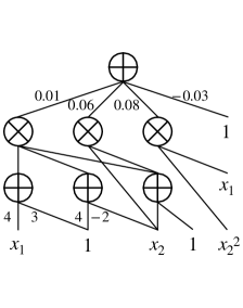
(a) PC for likelihood polynomial.

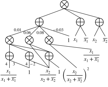
(b) Leaf nodes replaced with division gadgets.

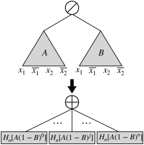
(c) top: A single division node.
bottom: Sum of homogeneous parts.

Figure 2: An example transforming a circuit representing a likelihood polynomial $p(x)=0.08x_{1}x_{2}+0.16x_{1}+0.12x_{2}+0.09$ to a circuit representing a network polynomial. First, (b) gadgets using division nodes are introduced at the leaves (as well as a multiplying factor) to obtain a rational function equivalent to the network polynomial. Then (c:top) all divisions are pushed to a single division node at the root so $p(x,\bar{x})=A/B$, and (c:bottom) a sum over necessary homogeneous parts of $A$ and $B$ is formed.

3 Network and likelihood polynomials

There are various polynomials containing all the information of a binary distribution $\Pr$, in the sense that any value $\Pr(\bm{x})$ can be recovered from the polynomial alone. It is known that efficient circuit representations of some such polynomials still allow tractable marginal inference, but a unified analysis of the various polynomial representations is lacking. In this section, we begin with the most studied such polynomial, the network polynomial, and establish its connections to the more natural – yet still, as we show, tractable – likelihood polynomial.

3.1 Network Polynomials

Darwiche [2003] showed that Bayesian Networks can be compiled to circuits computing a certain polynomial representation of their distribution which he called the network polynomial (also see [Castillo et al., 1995]). The network polynomial of binary probability distribution $\Pr$ is

$$p(x_{1},\ldots,x_{n},\bar{x}_{1},\ldots,\bar{x}_{n})=\sum_{S\subseteq[n]}\Pr(\bm{x}_{S})\prod_{i\in S}x_{i}\prod_{i\notin S}\bar{x}_{i}.$$ (1)

Significant work towards learning and applying circuits computing this polynomial has since been developed [Poon and Domingos, 2011, Peharz et al., 2020, Liu et al., 2021]. In particular, this is the canonical polynomial computed by circuits in the growing literature on Probabilistic Circuits (PC) [Choi et al., 2020]. The key feature of circuits computing network polynomials is that they enable linear time (and very simple!) marginal inference. We note that while algorithms for marginalization are typically given for smooth and decomposable circuits, the following Proposition holds for circuits of any structure which compute a network polynomial.

Proposition 1.

Computing marginals on a circuit of size $s$ representing a network polynomial takes $O(s)$ time. For the random variable assignment $X_{i}=1$, set $x_{i}=1$ and $\bar{x}_{i}=0$; for $X_{i}=0$, set $x_{i}=0$ and $\bar{x}_{i}=1$; marginalize $X_{i}$ by setting $x_{i}=\bar{x}_{i}=1$.

The network polynomial is a polynomial with very specific structure. First, the network polynomial is multilinear. Second, every monomial with a nonzero coefficient contains $x_{i}$ or $\bar{x}_{i}$ for every $i\in\{1,2,\ldots,n\}$. However, we wonder whether the structure of the monomials with variables $x_{i}$ and $\bar{x}_{i}$ is necessary for marginal inference. We next consider a definition which does not use these $\bar{x}_{i}$ variables but, as we show, remains tractable.

3.2 Likelihood Polynomials

Roth and Samdani [2009] considered perhaps the simplest polynomial representation of $\Pr$, that which directly computes $\Pr$ using variables $x_{1},\ldots,x_{n}$. Such a polynomial is obtained from a network polynomial by substituting $\bar{x}_{i}=1-x_{i}$ (transformation $2$ in Figure 1). We call this the likelihood polynomial:

$$p(x_{1},\ldots,x_{n})=\sum_{S\subseteq[n]}\Pr(\bm{x}_{S})\prod_{i\in S}x_{i}\prod_{i\notin S}(1-x_{i}).$$ (2)

While conceptually simple, it is not clear how or whether it is possible to efficiently compute marginals given a circuit representation of the likelihood polynomial. In particular, Roth and Samdani [2009] considered only “flat” representations of the likelihood polynomial, where all monomials with nonzero coefficients and their coefficients are stored explicitly. While marginal inference is linear in the size of the flat representation, there is an exponential gap in succinctness between circuits and flat representations.

We note that both network polynomials and likelihood polynomials are multilinear. Moreover, the standard structural property decomposability in the tractable circuits literature implies that the polynomial computed by a circuit is multilinear. Indeed, inference on circuits that agree with $\Pr$ on all inputs in $\{0,1\}^{n}$ becomes intractable without multilinearity. For example, if we just relax the restriction of multilinearity to circuits computing polynomials that are quadratic in each variable, marginal inference already becomes #P-hard (e.g. implicit in the proof of Theorem 2 in Khosravi et al. [2019]).

We show that given a circuit computing a likelihood polynomial, there is still a linear time marginal inference algorithm.

Proposition 2.

Marginal probabilities on a circuit of size $s$ representing a likelihood polynomial can be computed in time $O(s)$.

By definition, a circuit representing a likelihood polynomial computes

$$p(x_{1},\ldots,x_{n})=\sum_{S\subseteq[n]}\Pr(\bm{x}_{S})\prod_{i\in S}x_{i}\prod_{i\notin S}(1-x_{i}).$$ (3)

We observe that setting $x_{i}=\bar{x}_{i}=1$ in the following expression is equivalent to marginalizing in a network polynomial as in Proposition 1.

$$\prod_{i=1}^{n}(x_{i}+\bar{x}_{i})\cdot p\left(\frac{x_{1}}{x_{1}+\bar{x}_{1}},\ldots,\frac{x_{n}}{x_{n}+\bar{x}_{n}}\right)$$

$$=\prod_{i=1}^{n}(x_{i}+\bar{x}_{i})\sum_{S\subseteq[n]}\Pr(\bm{x}_{s})\prod_{i\in S}\frac{x_{i}}{x_{i}+\bar{x}_{i}}\prod_{i\notin S}\left(1-\frac{x_{i}}{x_{i}+\bar{x}_{i}}\right)$$

$$=\sum_{S\subseteq[n]}\Pr(\bm{x}_{s})\prod_{i\in S}x_{i}\prod_{i\notin S}\bar{x}_{i}$$

$$=p(x,\bar{x}).$$

In fact, this expression naturally corresponds to a circuit computing the network polynomial using division nodes; replace inputs $x_{i}$ with $x_{i}/(x_{i}+\bar{x}_{i})$ and multiply the whole circuit by $\prod_{i=1}^{n}(x_{i}+\bar{x}_{i})$. However, the probabilistic circuits literature does not typically use division nodes, and available software libraries and known algorithms would need to be reconsidered to use division nodes, not to mention possible divide-by-zero problems – which we will in fact see arise in Section 4. This leads to the question, can we find a circuit computing an equivalent polynomial without use of division nodes? Classic work in the circuit complexity theory literature by Strassen [1973] provides a positive answer.

Theorem 1 (Strassen).

If $C$ is an arithmetic circuit with division nodes of size $s$, computing polynomial $p$ of degree $d$ over an infinite field, then there exists an arithmetic circuit $C^{\prime}$ of size $\text{poly}(s,d,n)$ that computes $p$ using only addition and multiplication nodes.

In particular, we have the following Theorem, which corresponds to transformation $4$ in Figure 1.

Theorem 2.

Let $\Pr$ be a probability distribution on $n$ binary random variables. Then a circuit of size $s$ computing the likelihood polynomial for $\Pr$ can be transformed to a circuit of size $O(n^{2}s)$ computing the network polynomial for $\Pr$.

To illustrate the algorithm, we consider the running example in Figure 2. Figure 2(a) shows the initial circuit that represents the likelihood polynomial. Figure 2(b) shows the circuit computing the expression with division nodes. To remove division nodes, the first observation is that all division nodes can be moved ‘up’ to a single division at the output node using the identities $(a/b)\times(c/d)=(ac)/(bd)$ and $(a/b)+(c/d)=(ad+bc)/(bd)$, as visualized in Figure 2(c). At this point we have the network polynomial written as a ratio of two polynomials, $p(x,\bar{x})=A(x,\bar{x})/B(x,\bar{x})$. Without loss of generality we assume $B$ has constant term one, i.e. $B(0,0,\ldots,0)=1$.

One additional result from the circuit complexity theory literature is needed at this point; for any circuit $f$ of size $s$ and degree $d$, a circuit of size $O(d^{2}s)$ can be constructed (with $d+1$ outputs) computing $H_{0}[f],H_{1}[f],\ldots,H_{d}[f]$ where $H_{i}[f]$ has degree $i$ and $f=\sum_{i}H_{i}[f]$ [Shpilka and Yehudayoff, 2010]. This process is called homogenization, and the $H_{i}[f]$’s the homogeneous parts of $f$.

The final division node can now be eliminated by use of the common polynomial identity $\frac{a}{1-r}=\sum_{j=0}^{\infty}ar^{j}$. We have

$$p(x,\bar{x})=\frac{A}{B}=\frac{A}{1-(1-B)}=\sum_{j=0}^{\infty}A(1-B)^{j}.$$ (4)

In particular, these equalities hold for the homogeneous parts of $p(x,\bar{x})$. And, because $B(0,\ldots,0)=1$, we know that $1-B$ has constant term zero, and so all monomials in $(1-B)^{j}$ have degree at least $j$. Since we know that the network polynomial $p(x,\bar{x})$ has all terms of degree exactly $n$, we only need to compute

$$H_{n}[p(x,\bar{x})] =\sum_{j=0}^{n}H_{n}[A(1-B)^{j}],$$

as illustrated by Figure 2(c). In particular, a single circuit computing $(1-B)^{j}$ for $j\in\{0,1\ldots,n\}$ can be homogenized in addition to homogenizing $A$, to compute $p(x,\bar{x})$ with size $O(n^{2}s)$.

4 Generating Polynomials

So far we have considered circuits that directly compute a distribution. However, there are other well known polynomial representations of probability distributions which have been shown as promising representations for tractable probabilistic modeling. Zhang et al. [2021] consider circuits computing the Probability Generating Function of a distribution. Generating Functions are well studied in mathematics as theoretical objects [Wilf, 2005], but have recently been identified as useful data structures [Zhang et al., 2021, Klinkenberg et al., 2023, Zaiser et al., 2023]. The generating polynomial for probability distribution $\Pr$ is

$$g(x_{1},\ldots,x_{n})=\sum_{S\subseteq[n]}\Pr(\bm{x}_{s})\prod_{i\in S}x_{i}.$$ (5)

Zhang et al. [2021] call circuits computing generating polynomials Probabilistic Generating Circuits (PGCs) and show that marginal inference on PGCs is tractable. For a PGC of size $s$ in $n$ variables, they provide an $O(sn\log n\log\log n)$ marginal inference algorithm which has been improved by Harviainen et al. [2023] to $O(ns)$. It is also noted by Zhang et al. [2021] that circuits computing network polynomials can be transformed to PGCs simply by replacing $\bar{x}_{i}$’s by $1$, and so any distribution with a polynomial-size circuit computing its network polynomial also has a polynomial-size PGC; this is transformation $2$ in Figure 1. On the other hand, they show that there are distributions with polynomial-size PGCs but for which any decomposable circuit computing the network polynomial using only positive weights has exponential size (and additional PGC lower bounds are known Bläser [2023]). It is left as an open question whether this separation still holds for circuits with unrestricted weights. We settle this question with a negative answer. Using a method similar to that in Section 3, we show that given a PGC, one can find a circuit computing the network polynomial with a polynomial increase in size; this is transformation 1 in Figure 1.

Theorem 3.

Let $\Pr$ be a probability distribution on $n$ binary random variables. Then a circuit of size $s$ computing the probability generating function for $\Pr$ can be transformed to a circuit of size $O(n^{2}s)$ computing the network polynomial for $\Pr$.

Proof.

We obtain the desired circuit by first constructing a circuit that computes $p(x,\bar{x})$ using division nodes. Observe

$$\left(\prod_{i=1}^{n}\bar{x}_{i}\right)g\left(\frac{x_{1}}{\bar{x}_{1}},\frac{x_{2}}{\bar{x}_{2}},\ldots,\frac{x_{n}}{\bar{x}_{n}}\right)$$

$$\quad=\left(\prod_{i=1}^{n}\bar{x}_{i}\right)\sum_{S\subseteq[n]}\Pr(\bm{x}_{S})\prod_{i\in S}\frac{x_{i}}{\bar{x}_{i}}$$

$$\quad=\sum_{S\subseteq[n]}\Pr(\bm{x}_{S})\prod_{i\in S}x_{i}\prod_{i\notin S}\bar{x}_{i}$$

$$\quad=p(x_{1},\ldots,x_{n},\bar{x}_{1},\ldots,\bar{x}_{n})$$

The degree of $p(x,\bar{x})$ is $n$, and so using Theorem 1 as in Section 3, there is a circuit computing $p(x,\bar{x})$ without division nodes of size $O(n^{2}s)$. ∎

We note the similarity of the proof of Theorem 2 to that of Theorem 3. They both involve constructing a circuit to represent $p(x,\bar{x})$ initially using division nodes and then removing the division nodes. We also note the crucial difference between the proofs; in the construction for Theorem 3, the circuit with division nodes can not be used to evaluate $p(x,\bar{x})$ directly because it would require division by zero whenever $\bar{x}_{i}=0$ for any $i\in[n]$. Therefore the ability to remove divisions while maintaining equivalence of the polynomial computed is essential for this transformation to be meaningful. As one immediate consequence, this implies the existence of polynomial size PCs computing network polynomials for DPPs since Zhang et al. [2021] showed the existence of polynomial size PGCs for DPPs. Another practical benefit is that rather than using a bespoke polynomial-interpolation algorithm for inference in PGCs, there is a simple feedforward (and easily implemented, on a GPU for example) method of inference for PGCs after the transformation has been performed.

5 Fourier Transforms

Fourier analysis involves representing functions in the frequency domain and is ubiquitous across math and computer science. Yu et al. [2023] show that circuits representing Fourier transforms (called Characteristic Functions in Probability Theory) can improve learning in a mixed discrete-continuous setting while still supporting marginal inference when the circuit is smooth and decomposable (see Section 6 for discussion of these properties). Xue et al. [2016] show that Fourier representations can improve approximate inference in the binary setting too. The Fourier transform [O’Donnell, 2014] of pseudoboolean function $p:\{0,1\}^{n}\to\mathbb{R}$ is

$$\hat{p}(\bm{t})=2^{-n}\sum_{\bm{x}\in\{0,1\}^{n}}p(x)(-1)^{\langle\bm{t},\bm{x}\rangle}.$$ (6)

It is convenient that in this binary case, $\hat{p}$ can also be simply written as a multilinear polynomial (note that the equality holds on its domain $\{0,1\}^{n}$):

$$\hat{p}(t_{1},\ldots,t_{n})=2^{-n}\sum_{S\subseteq[n]}p(x_{S})\prod_{i\in S}(1-2t_{i}).$$ (7)

For the rest of the paper we use $\hat{p}$ to refer to this multilinear polynomial. We note that Fourier analysis of binary functions is a rich subject in its own right and refer the reader to O’Donnell [2014].

While there is no obvious connection between network polynomials, generating functions, and Fourier transforms, we show that in fact they are closely related. This relation hinges on switching between the domains $\{0,1\}^{n}$ and $\{-1,1\}^{n}$. In particular, we define for any polynomial $f$ its counterpart $f_{-1,1}$ as follows:

$$f_{-1,1}(x_{1},\ldots,x_{n})=f\left(\frac{1-x_{1}}{2},\ldots,\frac{1-x_{n}}{2}\right),$$ (8)

also a multilinear polynomial. Similarly, observe that we can write

$$f(x_{1},\ldots,x_{n})=f_{-1,1}\left(1-2x_{1},\ldots,1-2x_{n}\right).$$ (9)

Note that $f$ and $f_{-1,1}$ compute the same function on the respective domains $\{0,1\}^{n}$ and $\{-1,1\}^{n}$ up to the bijection $\phi:\{0,1\}\to\{-1,1\}$ given by $\phi(b)=(-1)^{b}$ applied bitwise. In particular, Equations 8 and 9 can be applied to circuits with modifications at only the leaves, giving the following lemma.

Lemma 1.

A circuit of size $s$ computing polynomial $f$ (resp. $f_{-1,1}$) can be transformed to a circuit of size $O(s)$ computing $f_{-1,1}$ (resp. $f$).

We now make a simple observation that connects Fourier transforms with generating polynomials; up to a constant factor, generating polynomials are Fourier transforms, written on the domain $\{-1,1\}^{n}$.

Proposition 3.

Let $\Pr:\{0,1\}^{n}\to\mathbb{R}$ be a probability distribution with generating polynomial $g$ and Fourier polynomial $\hat{p}_{-1,1}(x)$ on the domain $\{-1,1\}$. Then $g(x)=2^{n}\hat{p}_{-1,1}(x)$.

Proof.

$$g(x) =\sum_{S\subseteq[n]}\Pr(\bm{X}_{s})\prod_{i\in S}x_{i}$$

$$=\sum_{S\subseteq[n]}\Pr(\bm{X}_{S})\prod_{i\in S}\left(1-2\left(\frac{1-x_{1}}{2}\right)\right)$$

$$=2^{n}\hat{p}_{-1,1}(x).$$

∎

Using only the ability to switch between the domains $\{0,1\}^{n}$ and $\{-1,1\}^{n}$ and Proposition 3, we now have transformations $11$ and $12$ in Figure 1.

Theorem 4.

Let $\Pr$ be a probability distribution on $n$ binary random variables. Then a circuit of size $s$ computing the generating polynomial $g$ for $\Pr$ (resp. $\hat{p}$) can be transformed to a circuit of size $O(s)$ representing the Fourier transform $\hat{p}$ for $\Pr$ (resp. $g$).

Proof.

Proposition 3 and Lemma 1. ∎

Having observed this connection between generating polynomials and Fourier polynomials, we have completed a path between $p$ and $\hat{p}$ in Figure 1, i.e. a polynomial time transformation between circuits computing them. However, we point out that this path more naturally corresponds to computing the inverse Fourier transform, and there is a symmetric set of transformations that compute $\hat{p}$ from $p$ in a more natural way. In particular, it is more common to define the binary Fourier transform $\hat{p}$ of $p$ in terms of its Fourier expansion:

$$p(x) =\sum_{S\subseteq[n]}\hat{p}(x_{S})(-1)^{\sum_{i\in S}x_{i}}$$

$$=\sum_{S\subseteq[n]}\hat{p}(x_{S})\prod_{i\in S}(1-2x_{i})$$

where the last equality holds for inputs in $\{0,1\}^{n}$. When written in this form, it becomes clear that $\hat{p}$ computes the coefficients of $p$ when written as a linear combination of parity functions (specifically, $\hat{p}(x_{S})$ computes the coefficient of the parity function $\prod_{i\in S}(1-2x_{i})$). Note the equivalence of the functions $\prod_{i\in S}(1-2x_{i})$ to the monomials $\prod_{i\in S}x_{i}$ on the respective domains $\{0,1\}^{n}$ and $\{-1,1\}^{n}$, and then we have that $\hat{p}(x_{S})$ simply computes the coefficient of the monomial $\prod_{i\in S}x_{i}$ in $p_{-1,1}$. Thus, we can find $\hat{p}$ from $p$ by first transforming $p$ to $p_{-1,1}$ using Lemma 1 (transformations 5 and 7 in Figure 1). Then to obtain a polynomial which computes the coefficients of $p_{-1,1}$ we use the equivalent transformation from generating polynomials to network polynomials to obtain polynomial $\hat{p}_{-1,1}(x,\bar{x})$, and finally substituting $\bar{x}=1-x$ we obtain $\hat{p}(x)$; transformations 7 and 9 in Figure 1. Moreover, the reverse transforms can be obtained by the same methods in the ‘upper half’ of Figure 1 as well.

Having now completed the transformations presented in Figure 1, we ask how they simplify in the presence of structural constraints common in the tractable circuits literature.

6 Decomposability

So far we make no assumptions on the structural properties of PCs; in this section, we consider the special case where the PC is decomposable [Darwiche and Marquis, 2002], which is a common assumption that guarantees tractable marginals, and we show that in this case some of the transformations described before can be simplified. We use the scope of a node to refer to the set of all $i$ such that variables $x_{i}$ or $\bar{x}_{i}$ appear as inputs among its descendants and itself.

Definition 2 (Decomposability).

A product node is decomposable if its children have disjoint scopes. A circuit is decomposable if all its product nodes are decomposable.

Definition 3 (Smoothness).

A sum node in indeterminates $x$ and $\bar{x}$ is smooth if its children have equal scope. A circuit is smooth if all of its sum nodes are smooth.

Decomposability is a very common property because it guarantees multilinearity and, when paired with smoothness, guarantees tractable marginal inference by computing a network polynomial. In particular, it is well known that if a circuit is smooth and decomposable, it computes a network polynomial [Poon and Domingos, 2011, Choi et al., 2020]. We note that if a circuit is decomposable, then it can be made smooth efficiently (increasing the size at most by a linear factor Choi et al. [2020], and less for certain decomposable structures Shih et al. [2019]).

We now show how the transformations used for Theorems 2,3,4 can be simplified and improved for decomposable circuits. First, we show that in decomposable circuits Fourier transforms correspond to trivial modifications at only the leaves.

Theorem 5.

A decomposable circuit of size $s$ representing a likelihood polynomial $p$ can be transformed to a decomposable circuit of size $O(s)$ representing a Fourier transform $\hat{p}$ by only modifications to the leaves.

Sketch.

A circuit representing $\hat{p}$ can be constructed with modifications pushed entirely to the leaves inductively. Essentially, decomposability allows Fourier transforms to be pushed to the children of each product node; transforms are also straightforwardly pushed to children of sum nodes. Finally, leaf nodes are univariate and so can be transformed trivially. ∎

Transformations $1$ and $4$ in Figure 1 can be simplified when the initial circuits are decomposable; the decomposability is preserved during the transformation, and the worst-case increase in size is lowered to $O(ns)$. First, a decomposable circuit of size $s$ computing a likelihood polynomial $p$ can be transformed to decomposable circuit of size $O(ns)$ computing $p(x,\bar{x})$. We note that this problem is exactly that of smoothing [Shih et al., 2019, Choi et al., 2020] and so the following lemma is included for completeness but is already known. In particular, this shows how Theorem 2 can be viewed as a generalization of smoothing to circuits without decomposability.

Lemma 2.

A decomposable circuit of size $s$ computing likelihood polynomial $p(x)$ can be transformed to a decomposable circuit of size $O(ns)$ computing network polynomial $p(x,\bar{x})$.

Next, we also have that a decomposable circuit of size $s$ computing a generating polynomial $g$ can be transformed to decomposable circuit of size $O(ns)$ computing $p(x,\bar{x})$. This problem, while not smoothing, can be solved by a similar approach; rather than smoothing with gadgets computing $x_{i}+\bar{x_{i}}$, simply use $\bar{x_{i}}$.

Lemma 3.

A decomposable circuit of size $s$ computing generating polynomial $g(x)$ can be transformed to a decomposable circuit of size $O(ns)$ computing network polynomial $p(x,\bar{x})$.

We note that Lemmas 2 and 3 hold for the symmetric transformations as described in Section 5; in particular, for decomposable versions of transformations $7$ and $10$ in Figure 1.

7 Categorical Distributions

So far we have considered binary probability distributions, functions of the form $\Pr:\{0,1\}^{n}\to\mathbb{R}$. Of course, categorical distributions of the form $\Pr:S^{n}\to\mathbb{R}$ for arbitrary finite set $S$ are also of interest. In the PC literature, categorical distributions are typically encoded as binary distributions using binary indicator variables [Darwiche, 2003, Poon and Domingos, 2011, Choi et al., 2020]. Indeed, the polynomials in this paper have no other straightforward and potentially tractable extension to the categorical setting, with one exception: generating polynomials. In fact, the generating polynomials considered in Zhang et al. [2021] are a restriction to the binary case of the following more general and standard definition. Let $\Pr:K^{n}\to\mathbb{R}$ be a probability distribution for $K=\{0,1,2,\ldots,k-1\}$ where we call the elements of $\{0,1,2,\ldots,k-1\}$ categories. Then the probability generating polynomial of $\Pr$ is

$$g(x)=\sum_{(d_{1},d_{2},\ldots,d_{n})\in K^{n}}\Pr(d_{1},\ldots,d_{n})x_{1}^{d_{1}}x_{2}^{d_{2}}\cdots x_{n}^{d_{n}}.$$ (10)

It is then natural to consider a categorical PGC as a circuit computing the generating function of a categorical distribution with more than two categories. This begs the question, are categorical PGCs a tractable model? To this, we give a negative answer. In fact, not only are marginals hard, but even likelihoods.

Theorem 6.

Computing likelihoods on a categorical PGC is #P-hard for $k>3$ categories.

$\pNiceMatrix[margin]0&100\\ 0100\\ 0100\\ 0100\\ \to\pNiceMatrix[margin]0&1\Block[fill=blue!15,rounded-corners]{5-1}{}000\\ 01000\\ \Block[fill=blue!15,rounded-corners]{1-5}{}0\underline{1}\underline{1}00\\ 00\underline{\underline{1}}00\\ 00\underline{\underline{1}}00\\$

Figure 3: An example of the permanent-preserving operation used to make $M$ sparse. The new row and column are shaded in blue. The newly-added nonzero entries are singly-underlined. The nonzero entries that moved from their original column to the new one are doubly-underlined.

We prove Theorem 6 by a reduction from the $\{0,1\}$-Permanent to categorical PGC inference. The classic work of Valiant [1979b] shows that computing the permanent of matrices with entries in $\{0,1\}$ is #P-hard. The permanent of a matrix $M$ is

$$\text{per\,}M=\sum_{\sigma\in S_{n}}\prod_{i=1}^{n}M_{i,\sigma(i)}$$

where $S_{n}$ is the symmetric group of order $n$.

Our reduction proceeds in two steps. Let $M\in\{0,1\}^{n\times n}$. We first find a slightly larger but sparse matrix $M^{\prime}$ such that $\text{per\,}M=\text{per\,}M^{\prime}$. Then, we use a polynomial construction from Valiant [1979a], Koiran and Perifel [2007] to obtain a categorical PGC for which computing a single likelihood would equivallently compute $\text{per\,}M$.

1. Let $M\in\{0,1\}^{n\times n}$. Suppose the $i$th column of $M$ contains more than three nonzero entries. Insert a new row and column between the original $i$ and $(i+1)$th rows and columns respectively, setting their $(i+1)$th entries (i.e. their shared value on the main diagonal) to $1$. Also set the $i$th entry of the new row to $1$. Now select any two of the original nonzero entries of the $i$th column and move them to the new $(i+1)$th column (i.e. if they have index $j$ and $j^{\prime}$ in column $i$, set $M_{j,i}=M_{j^{\prime},i}=0$ and $M_{j,i+1}=M_{j^{\prime},i+1}=1$). Call the resulting matrix $M^{\prime}$ and observe that $\text{per\,}M=\text{per\,}M^{\prime}$. Figure 3 gives an example of this transformation. Repeat this permanent-preserving operation until all columns contain at most three nonzero entries, which requires at most $n^{2}$ repetitions.

2. Let $n^{\prime}$ be the new size of $M^{\prime}$ (i.e. $M^{\prime}\in\{0,1\}^{n^{\prime}\times n^{\prime}}$). We now simply construct a circuit $g(x)$ computing

   $$\prod_{i=1}^{n^{\prime}}\sum_{j=1}^{n^{\prime}}M^{\prime}_{i,j}x_{j}.$$ (11)

   Observe that the coefficient of the the monomial $\prod_{i=1}^{n^{\prime}}x_{i}$ in $g(x)$ is exactly $\text{per\,}M^{\prime}=\text{per\,}M$. Thus with $g(x)$ interpreted as a categorical PGC, the likelihood query with $X_{1}=X_{2}=\ldots=X_{n^{\prime}}=1$ computes $\text{per\,}M$.

This motivates the need to research tractable categorical distributions, e.g. possibly in the direction suggested by Cao et al. [2023]. In particular, this calls for careful consideration of the use of generating functions over categorical variables, which are not tractable models in general.

8 Conclusion

We studied tractable probabilistic circuits computing various polynomial representations of probability distributions. For binary probability distributions we show that a number of previously studied polynomials have equivalently expressive-efficient circuit representations. Among circuits computing network, likelihood, generating, and Fourier polynomials, all support tractable marginal inference, and, given a circuit computing any one polynomial, a circuit computing any other can be obtained with at most a polynomial increase in size. This establishes a relationship between several previously-independent marginal inference algorithms, and establishes one novel marginal inference algorithm, namely for circuits computing likelihood polynomials. These results connect well-studied mathematical objects like generating functions and Fourier transforms in their forms as tractable probabilistic circuits, opening up potential future research, for example leveraging theory developed in one semantics and translating it to another, or learning in one representation space and transforming to another.

Appendix A Proofs

Proof of Lemma 5.

Proof.

We construct $\hat{p}$ inductively as follows. For a product node, we have $\hat{p}(t)=\hat{p}_{0}(t_{0})\hat{p}_{1}(t_{1})$, and so

$$p(x) =\sum_{t\in\{0,1\}^{n}}\hat{p}(t)(-1)^{\langle t,x\rangle}$$

$$=\sum_{t\in\{0,1\}^{n}}\hat{p}_{0}(t_{0})\hat{p}_{1}(t_{1})(-1)^{\langle t,x\rangle}$$

$$=\left(\sum_{t_{0}\in\{0,1\}^{n}}\hat{p}_{0}(t_{0})(-1)^{\langle t_{0},x_{0}\rangle}\right)\cdot\left(\sum_{t_{1}\in\{0,1\}^{n}}\hat{p}_{1}(t_{1})(-1)^{\langle t_{1},x_{1}\rangle}\right)$$

$$=p_{0}(x_{0})p_{1}(x_{1})$$

where the first equality follows from definition, the second from the hypothesis, the third from algebra, and the final from definition. For a sum node, we have $\hat{p}(t)=\sum_{i}w_{i}\hat{p_{i}}(t)$, and so

$$p(x) =\sum_{t\in\{0,1\}^{n}}\hat{p}(t)(-1)^{\langle t,x\rangle}$$

$$=\sum_{t\in\{0,1\}^{n}}\left(\sum_{i}w_{i}\hat{p}_{i}(t)\right)(-1)^{\langle t,x\rangle}$$

$$=\sum_{i}w_{i}\sum_{t\in\{0,1\}^{n}}\hat{p}_{i}(t)(-1)^{\langle t,x\rangle}$$

$$=\sum_{i}w_{i}p_{i}(x)$$

where the equalities follow, respectively, from definition, assumption, commutativity of addition, and definition.

For leaf nodes, it suffices to consider only univariate leaves that are children of sums; for any leaf a child of a product node, add a sum node with weight $1$ between them. Then, for a univariate child of a sum node with scope the singleton $\{i\}$, we have either $p(x_{i})=c$, and so

$$\hat{p}(t_{i}) =\sum_{S\subseteq[n]}p(x_{S})\prod_{i\in S}(1-2t_{i})$$

$$=2^{-n}(c+c(1-2x_{i}))=2^{-n+1}c(1-x_{i})$$

or $p(x_{i})=x_{i}$, in which case

$$\hat{p}(t_{i})=\sum_{S\subseteq[n]}p(x_{S})\prod_{i\in S}(1-2t_{i})=2^{-n}(1-2x_{i}).$$ (12)

∎