Sobolev Training for Operator Learning

Abstract

This study investigates the impact of Sobolev Training on operator learning frameworks for improving model performance. Our research reveals that integrating derivative information into the loss function enhances the training process, and we propose a novel framework to approximate derivatives on irregular meshes in operator learning. Our findings are supported by both experimental evidence and theoretical analysis. This demonstrates the effectiveness of Sobolev Training in approximating the solution operators between infinite-dimensional spaces.

1 Introduction

Over the last few decades, machine learning has seen substantial advancements in various areas, such as computer vision (Dosovitskiy et al., 2020; Niemeyer & Geiger, 2021), natural language processing (Vaswani et al., 2017; Radford et al., 2018; Lewis et al., 2019; Kenton & Toutanova, 2019), and physical modeling (Raissi et al., 2019; Jagtap & Karniadakis, 2020). In physical modeling, machine learning methods are valuable tools for solving complex partial differential equations (PDEs). An emerging field within this domain is operator learning, which uses neural networks to learn mappings between infinite-dimensional spaces.

By utilizing the expressive power of neural networks, neural operators can be trained using datasets of input and output functions. Once trained, these operators can predict unseen equations with just a single forward computation. Compared to classical FDM/FEM methods, these ML-based methods greatly accelerate the equation-solving process. In the field of operator learning, FNO (Li et al., 2021) and DeepONet (Lu et al., 2021) are the most popular models. For a comprehensive overview, we refer to (Kovachki et al., 2021; Hao et al., 2022; Zappala et al., 2021) and the references therein.

Sobolev Training, introduced in (Czarnecki et al., 2017), enhances traditional training methods by integrating the derivatives of the target function along with its values. This method improves the accuracy of predictions and boosts data efficiency and the model’s generalization ability in function approximation. The authors of (Czarnecki et al., 2017) provide theoretical and empirical validation for these improvements.

A recent and significant application of Sobolev Training can be seen in Physics-Informed Neural Networks (PINNs). Sobolev-PINNs, introduced in (Son et al., 2023), represent an adaptation of Sobolev Training. This is achieved by designing a novel loss function that directs the neural network to minimize errors within the corresponding Sobolev space. Empirical evidence has demonstrated that Sobolev-PINNs accelerate the convergence rate in solving complex PDEs. Furthermore, the authors of (Son et al., 2023) provide theoretical justifications for guaranteeing convergence in several equations.

Motivated by the previously mentioned works, we propose the Sobolev Training method for operator learning and provide theoretical and experimental support for its efficacy.

Here are the two significant challenges in our work. First, there is a need to approximate derivatives on irregular meshes to apply the Sobolev Training method to various existing models, as most recent results involve irregular meshes. To address this challenge, we adopt a local approximation method using moving least squares (MLS) within a coordinate system that is locally constructed. This system is derived from local principal component analysis (PCA) utilizing K-nearest neighbors (KNN), as developed in (Lipman et al., 2006; Liang & Zhao, 2013).

Second, the solution operator of PDEs exhibits non-local properties, which can be described using an integral operator. This approach requires additional work in theoretical analysis. Motivated by the work of (Tian, 2017), we provide a convergence analysis for a single layer with ReLU activation when the target function is described using an integral operation. We prove that including derivatives in the loss function improves convergence speed. To the best of our knowledge, this is the first work to present a convergence analysis in the context of operator learning, even without Sobolev Training. Furthermore, we show empirical evidence that PCgrad, introduced in (Yu et al., 2020), works well with the Sobolev Training method and enhances the performance of existing models.

Our contributions in this work are summarized as follows:

• Integration of a derivative approximation algorithm with existing operator learning models.

• Presentation of the first theoretical analysis on convergence in the field of operator learning.

• Introduction of Sobolev Training within operator learning, supported by theoretical and empirical evidence.

2 Preliminaries

2.1 Notations

Let us begin with the notations that are used throughout this paper. Given a multi-index $\alpha=(\alpha_{1},\cdots,\alpha_{n})\in(\mathbb{N}\cup\{0\})^{n}$ and a vector $x=(x^{1},\cdots,x^{n})\in\mathbb{R}^{n}$, we use $x^{\alpha}$ to denote

$$x^{\alpha}=(x^{1})^{\alpha_{1}}(x^{2})^{\alpha_{2}}\cdots(x^{n})^{\alpha_{n}}.$$

We define $|\alpha|=\alpha_{1}+\alpha_{2}+\cdots+\alpha_{n}$. Let $\Omega$ be a bounded domain in $\mathbb{R}^{n}$. The space of continuously differentiable functions up to order $M\in\mathbb{N}$ on $\Omega$ is denoted by $C^{M}(\Omega)$.

2.2 Sobolev spaces and Sobolev Training

Sobolev spaces are fundamental function spaces that appear in analyzing PDEs and functional analysis. For any $\varphi\in C^{|\alpha|}(\Omega)$, we denote

$$D^{\alpha}_{x}\varphi=\frac{\partial^{\alpha_{1}}}{\partial x^{1}}\cdots\frac{\partial^{\alpha_{n}}}{\partial x^{n}}\varphi.$$

For a given $u\in L^{p}(\Omega)$, if there exists $w\in L^{p}(\Omega)$ satisfyng

$$\int_{\Omega}uD_{x}^{\alpha}\xi\,dx=(-1)^{|\alpha|}\int_{\Omega}w\xi\,dx\quad\forall\varphi\in C^{\infty}_{0}(\Omega),$$

then we refer $w$ as the $\alpha^{th}$-weak derivative of $u$ and denote $w=D_{x}^{\alpha}u$. Unless otherwise specified, we use weak derivatives throughout this paper. We refer to Chapter 5 of (Evans, 2022) for detailed information regarding the Sobolev spaces. For $k\in\mathbb{N}$ and $1\leq p<\infty$, we define a Sobole space $W^{k,p}(\Omega)$ by

$$W^{k,p}(\Omega):=\{u\in L^{p}(\Omega):|D^{\alpha}_{x}u|\in L^{p}(\Omega)\ \ \forall|\alpha|\leq k\}.$$

The idea of training using Sobolev spaces is introduced in (Czarnecki et al., 2017). For a given function $f:\mathbb{R}^{n}\to\mathbb{R}^{m}$ with training set consisting of pairs ${(x_{j},f(x_{j}))}_{j=1}^{J}$, training a neural network $g_{\theta}(x)$ consists of finding $\theta$ that minimizes

$$\sum_{j=1}^{J}l(g_{\theta}(x_{j}),f(x_{j})),$$

for some given loss function $l$. In Sobolev Training, the loss function above is replaced by

$$\sum_{j=1}^{J}\left[l(g_{\theta}(x_{j}),f(x_{j}))+\sum_{i=1}^{n}l_{i}(D_{x}^{e_{i}}g_{\theta}(x_{j}),D_{x}^{e_{i}}f(x_{j}))\right],$$

where $D_{x}^{e_{i}}$ is the derivative of function in $i^{th}$ variable and $l_{i}$ is a loss function measuring error for each $i\in[1,\cdots,n]$.

2.3 Operator Learning

Operator learning is an emerging area of study in machine learning that employs neural networks to train solution operators for various equations. The DeepONet (Lu et al., 2021) and FNO (Li et al., 2021) are considered fundamental models in the field of operator learning. FNO efficiently learns complex PDEs using Fourier analysis. At the same time, DeepONet is a model developed based on the Universal Approximation Theorem for operators that can handle many problems, including multiple input functions and complex boundary conditions. However, like other data-driven methods, DeepONet requires substantial data. Many efforts have been made to improve existing models. Let us introduce some of the notable developments in several studies. For example, Geo-FNO (Li et al., 2022) is developed to expand the FNO model to solve equations with irregular meshes in FNO. The transformer architecture, introduced in (Vaswani et al., 2017), has achieved significant success in various fields such as natural language processing (Kenton & Toutanova, 2019; Radford et al., 2018) and computer vision (Dosovitskiy et al., 2020). In (Cao, 2021), the transformer is applied to operator learning, emphasizing the importance of selecting the appropriate transformer model. Recently, authors of (Hao et al., 2023) apply advanced machine learning techniques to transformer-based models. This approach enables handling diverse and complex datasets, resulting in more robust and scalable models.

2.4 Results on the convergence analysis

The convergence analysis of gradient descent has been rigorously studied in deep learning research. Convergence studies, particularly for linear models, serve as fundamental building blocks in understanding the behavior of gradient descent in complex architectures. In the notable works (Arora et al., 2018; Bartlett et al., 2018), authors provide theoretical insights into linear models. Parallel to these, authors of (Liu et al., 2020) investigate stochastic gradient methods with momentum (SGDM) and theoretically show improved convergence results compared to the usual stochastic gradient method. The convergence dynamics in two-layer neural networks with ReLU activation are explored extensively in (Tian, 2017; Li & Yuan, 2017). In particular, (Tian, 2017) explores population gradients, where the inputs are drawn from zero-mean spherical Gaussian distributions, and establishes interesting theoretical results, including the properties of critical points and the probability of convergence to the optimal weights with randomly initialized parameters. Such comprehensive studies collectively enhance our understanding of the intricate convergence behaviors in more complicated and larger neural network structures.

3 Proposed method

This section introduces our method and theoretical result for the Sobolev Training for operator learning.

3.1 Approximating derivatives in non-uniform meshes

We adopt the reconstructing local surface approximation method using the moving least-square (MLS) method developed in (Liang & Zhao, 2013; Lipman et al., 2006).

Let us assume that a function $u:\Omega\subset\mathbb{R}^{n}\to\mathbb{R}$ and a irregular mesh $\{x_{j}\}_{j=1}^{J}\subset\Omega$ are given. We denote by $\Pi_{m}^{n}$ the set of $n$-dimensional polynomial functions with a maximum degree less than or equal to $m$. For now, let us fix $\bar{x}\in\{x_{j}\}_{j=1}^{J}$. We then find $K$-nearest points of $\bar{x}$ denoted by $\{\bar{x}_{1},\bar{x}_{2},\cdots,\bar{x}_{K}\}\subset\{x_{j}\}_{j=1}^{J}$. We intend to solve the following minimization problem

$$\min_{p\in\Pi_{m}^{n}}\sum_{k=1}^{K}\omega(\|\bar{x}_{k}-\bar{x}\|)\|p(\bar{x}_{k})-u(\bar{x})\|^{2},$$ (1)

where $\omega(\cdot)$ is some weight function to be determined. In this work, we use the Equation 15. It is directly checked that the number of the biasis $\Pi_{m}^{n}$ is $I:=\frac{(m+n)!}{m!n!}$. Let $b(x)$ represent a polynomial basis vector, with each element of $b(x)$ denoted by $(x-\bar{x})^{\alpha}$ for any multi-index $\alpha$ satisfying $|\alpha|\leq m$. We denote $c\in\mathbb{R}^{I}$ by the coefficient vector of dimension $I$, and $c_{\alpha}$ represents the coefficient corresponding to $(x-\bar{x})^{\alpha}$. Each element in $\Pi_{m}^{n}$ can be expressed as

$$p(x)=c^{T}b(x)=c\cdot b(x)=\sum_{|\alpha|\leq m}c_{\alpha}(x-\bar{x})^{\alpha}.$$ (2)

By taking partial derivative in Equation 1, the coefficients can be determined by

$$c=E^{-1}\sum_{k=1}^{K}\omega(\|\bar{x}_{k}-\bar{x}\|)b(\bar{x}_{k})u(\bar{x}_{k}),$$ (3)

$$\text{with }E=\left(\sum_{k=1}^{K}\omega(\|\bar{x}_{k}-\bar{x}\|)b(\bar{x}_{k})b(\bar{x}_{k})^{T}\right).$$

Now, consider a set of data points $\{x_{j},u(x_{j})\}_{j=1}^{J}$. To solve the minimizing problem described in Equation 1, we apply Equation 3, substituting $\bar{x}$ with each $x_{j}$ in the dataset. Subsequently, the approximation of $D_{x}^{\alpha}(x_{j})u$ is represented by $c_{j,\alpha}$, which is the coefficient of $(x-x_{j})^{\alpha}$ for each polynomial. We summarize overall in Algorithm 1.

Algorithm 1 Estimating derivatives in non-uniform meshes

  Define: K: number of nearest points

  Define: m: polynomial order degree

  Input: $\{(x_{j},u(x_{j})\}_{j=1}^{J},K,m$

  Find $K$ nearest points for each $x_{j}$: $x_{KNN,j}:=(x_{KNN,j,1},\cdots,x_{KNN,j,K})$.

  Define a polynomial $p_{j}(x)$ for each $j$ defined by Equation 2

  Calculate coefficient vector $c_{j}\in\mathbb{R}^{I}$ using Equation 3

  Return: coefficient vector $c_{j}$ for each $i$.

In the following lemma, we prove that the result of Algorithm 1 indeed approximates the derivative of the target function in the Sobolev space. To this end, we assume that the data points $\{x_{j}\}_{j=1}^{J}$ are uniformly sampled so that

$$\frac{1}{J}\sum_{j=1}^{J}|f(\tilde{x}_{i})|^{2}\stackrel{{\scriptstyle C_{0}}}{{\approx}}\frac{1}{|\Omega|}\int_{\Omega}|f|^{2}\,dx,$$ (4)

where $C_{0}>0$ is some universal constant. In this context, for each $j$, $\tilde{x}_{j}$ denotes any point near $x_{j}$, satisfying the condition $\|x_{j}-\tilde{x}_{j}\|\leq\varepsilon$, where $\varepsilon>0$ is sufficiently small. For more details on the Monte-Carlo integration method, refer to (Press, 2007; Newman & Barkema, 1999).

Lemma 3.1.

Suppose $u\in W^{M,2}(D)$ for some $M\in\mathbb{N}$, and consider a set of grid points $\{x_{j}\}_{j=1}^{J}$ satisfing the Monte-Carlo approximation assumption Equation 4 for all $D^{\alpha}_{x}u$ with $|\alpha|\leq M$ and for some $C_{0}>0$. Define

$$h=\min_{j,k}\|x_{j}-x_{\text{KNN},j,k}\|,$$

and let $c_{j}$ be the coefficient vector obtained from Algorithm 1. Then, for all $m\leq M$, there exists a constant $C=C(C_{0},N,K,m,M,|\Omega|)$ such that the following inequality holds:

$$\frac{1}{J}\sum_{j=1}^{J}\sum_{|\alpha|=m}\|c_{j,\alpha}-D^{\alpha}u(x_{j})\|^{2}\leq Ch^{M-m}\|u\|_{W^{M,2}(\Omega)}.$$

In this context, we use $c_{j,\alpha}$ to denote the element of $c_{j}$ from Algorithm 1, corresponding to the $(x-x_{j})^{\alpha}\in\Pi_{m}^{n}$.

The proof can be found in Appendix C.1

3.2 Convergence analysis for the Sobolev Training for operator learning

This subsection provides theoretical evidence of the effectiveness of Sobolev Training in operator learning. Suppose that the query points $\{x_{j}\}_{j=1}^{J}$ is given from spherical Gaussian distribution, $\mathcal{N}(0,I)$. Suppose $\{u_{k}(x),v_{k}(x)\}_{k=1}^{N}$ is a pair of input and output real-valued functions. To capture non-local properties of the solution operator of PDEs, the solution can be described as an integral operator. We further assume that there exists $\{y_{l}\}_{l=1}^{\tilde{J}}$ such that

$$u_{k}(x) =\frac{1}{|\Omega|}\int_{\Omega}\kappa(x,y)v_{k}(y)\,dy$$ (5)

$$\approx\frac{1}{\tilde{J}}\sum_{l=1}^{\tilde{J}}\kappa(x,y_{l})v_{k}(y_{l})$$

for some kernel function $\kappa(x,y)$. The kernel function $\kappa(x,y)$ can be represented as

$$\kappa(x,y)=\sum_{\tilde{i}=1}^{\tilde{I}}\varphi^{\tilde{i}}(x)\psi^{\tilde{i}}(y),$$ (6)

where each $\varphi^{\tilde{i}}$ and $\psi^{\tilde{i}}$ is a neural network. For simplicity, we assume that

$$\tilde{I}=1\quad\text{and}\quad\varphi(x)=\psi(x)=\sigma(w^{T}x)$$ (7)

for some parameter $w\in\mathbb{R}^{n}$ and the activation function, $\sigma$ is the ReLu function. By the Universal Approximation Theorem (Lu et al., 2017), a two-layer network can approximate each $v_{k}\in W^{1,2}(\Omega)\subset L^{2}(\Omega)$. For the analytic simplicity, we suppose that

$$v_{k}(x)=\mu_{k}\sigma((w^{*})^{T}x)\quad\text{for some }w^{*}\in\mathbb{R}^{n}.$$ (8)

From these assumptions above, we have

$$u_{k}(x;w)=\frac{1}{\tilde{J}}\sum_{l=1}^{\tilde{J}}\mu_{k}\sigma(w^{T}x)\sigma(w^{T}y_{l})\sigma((w^{*})^{T}x).$$

By denoting $X=[x_{1},\cdots,x_{J}]\in\mathbb{R}^{J\times n}$, the usual $L^{2}$ loss function can be expressed as

$$\mathcal{L}_{L^{2}}=\frac{1}{N}\sum_{k=1}^{N}\left|u_{k}(X;w)-u_{k}(X;w^{*})\right|^{2}.$$ (9)

For the Sobolev Training, we denote

$$\mathcal{L}_{Der}=\frac{1}{N}\sum_{k=1}^{N}\left|D_{x}u_{k}(X;w)-D_{x}u_{k}(X;w^{*})\right|^{2}$$ (10)

and use the loss function

$$\mathcal{L}_{Sob} =\mathcal{L}_{L^{2}}+\mathcal{L}_{Der}.$$ (11)

For each training method given the initial parameter $w_{0}\in\mathbb{R}^{n}$, the parameters $w$ are updated via the following gradient descent method for some $t>0$

$$w_{L^{2}} =w_{0}-t\mathbb{E}_{X}\left[\frac{\partial\mathcal{L}_{L^{2}}}{\partial w}\right],$$ (12)

$$w_{Sob} =w_{0}-t\mathbb{E}_{X}\left[\frac{\partial\mathcal{L}_{Sob}}{\partial w}\right].$$

By taking $t\to 0$ in Equation 12, we have the following gradient flow:

$$\frac{dw_{L^{2}}}{dt} =-\mathbb{E}_{X}\left[\frac{\partial\mathcal{L}_{L^{2}}}{\partial w}\right],$$ (13)

$$\frac{dw_{Sob}}{dt} =-\mathbb{E}_{X}\left[\frac{\partial\mathcal{L}_{Sob}}{\partial w}\right].$$

Now, we are ready to present our main theorem.

Theorem 3.2.

Suppose that we are under the assumption Equations 5, 6, 7 and 8 and the activation function, $\sigma(x)$ is $ReLU(x)=\max(0,x)$. Also, let $w_{L^{2}}$ and $w_{Sob}$ be parameter vectors defined as Equation 13. Then, we have the following results:

• If $w_{0}:=w(0)\in\{w:\|w_{L^{2}}-w^{*}\|<\|w^{*}\|\}$, then

  $$\frac{d}{dt}\|w_{L^{2}}-w^{*}\|^{2}<0.$$

  Moreover, we have the convergence results $w_{L^{2}}\to w^{*}$ as $t\to\infty$.

• Under the same assumption as in the previous statement, we have

  $$\frac{d}{dt}\|w_{Sob}-w^{*}\|^{2}\leq\frac{d}{dt}\|w_{L^{2}}-w^{*}\|^{2}<0.$$

  In particular, if $w$ and $w^{*}$ is not parallel, that is if the angle between $w$ and $w^{*}$ is not $0$ and $\pi$, then we have

  $$\frac{d}{dt}\|w_{Sob}-w^{*}\|^{2}<\frac{d}{dt}\|w_{L^{2}}-w^{*}\|^{2}<0.$$ (14)

The proof can be found in Appendix C.2

3.3 Sobolev Training with PCGrad

The loss function, Equation 11, takes the form of a linear summation of two terms, $\mathcal{L}_{L^{2}}$ and $\mathcal{L}_{Der}$. It can be seen as a double-task objective, encompassing the prediction of $u$ and its derivatives. Learning two tasks simultaneously may lead to instability during training, especially when there are conflicting gradients—indicating gradients with opposite directions— or a substantial difference in gradient magnitudes (Yu et al., 2020).

To address these issues, we adopt PCGrad (Yu et al., 2020) during training, a technique designed to address multi-task learning scenarios. Here, we briefly explain how to apply PCGrad to our framework.

Let $\mathbf{g}_{1}:=\partial\mathcal{L}_{L^{2}}/\partial w$ and $\mathbf{g}_{2}:=\partial\mathcal{L}_{Der}/\partial w$, respectively. We say $\mathbf{g}_{1}$ and $\mathbf{g}_{2}$ are in conflict if they are in opposite directions, namely $\mathbf{g}_{1}\cdot\mathbf{g}_{2}<0$. When $\mathbf{g}_{1}$ and $\mathbf{g}_{2}$ are not in conflict, the parameters are updated by using the gradient $\mathbf{g}:=\mathbf{g}_{1}+\mathbf{g}_{2}$ as usual. If $\mathbf{g}_{1}$ and $\mathbf{g}_{2}$ are in conflict, however, we replace $\mathbf{g}_{2}$ with $\mathbf{g}_{2}-(\mathbf{g}_{1}\cdot\mathbf{g}_{2}/|\mathbf{g}_{1}|^{2})\mathbf{g}_{1}$, essentially subtracting the projection of $\mathbf{g}_{2}$ onto $\mathbf{g}_{1}$ from $\mathbf{g}_{2}$ or vice versa. This subtraction of the projection ensures that $\mathbf{g}_{1}$ and $\mathbf{g}_{2}$ are no longer in conflict, resulting in a more stable update of parameters.

In Section 4.2.5, we conduct an ablation study for the presence and absence of PCGrad in our framework. Specifically, we compare the cases of directly optimizing Equation 11 and applying PCGrad. It is experimentally confirmed that applying PCGrad performs better than not applying it. More details are in Section 4.2.5.

4 Experiments

In this section, we present a variety of experiments to demonstrate the effectiveness of the proposed framework. We compare the performance between the presence and absence of our framework. All the experiments are performed utilizing PyTorch 1.18.0 on Intel(R) Core(TM) i9-10980XE CPU at 3.00GHz and Nvidia GA102GL [RTX A5000].

Baseline models

We perform experiments on four baselines models: FNO (Li et al., 2021), Galerkin Transformer (Cao, 2021), GeoFNO (Li et al., 2022), and GNOT (Hao et al., 2023) with following datasets. We set $K=20$ and $m=2$, respectively. More details in the choice of $K$ and $m$ are described in Sections 4.2.2 and 4.2.3. We always set all other implementation details, e.g., each model’s number of hidden layers and selections of activation functions, to their default settings.

Datasets

We adopt six benchmark dataset as following: Darcy2d (Li et al., 2021), NS2d (Li et al., 2021), NACA (Li et al., 2022), Elasticity (Li et al., 2022), NS2d-c (Hao et al., 2023), and Heat (Hao et al., 2023).

Please refer to (Li et al., 2021; Cao, 2021; Li et al., 2022; Hao et al., 2023) for more details in baselines and models.

Error Criteria

In this section, we present an error analysis, adopting the relative errors in $L_{2}$-norm as the error criteria, formulated as follows:

$$\frac{1}{{N}_{D}}\sum\limits_{i=1}^{{N}_{D}}\frac{{\|\mathbf{u}^{NN}_{i}-\mathbf{u}_{i}\|}_{2}}{{\|\mathbf{u}_{i}\|}_{2}},$$

where ${N}_{D}$ is the dataset size, $\mathbf{u}^{NN}_{i}$ and $\mathbf{u}_{i}$ represent the predicted solutions and the target solutions for $i$th data, respectively.

4.1 Main Results

Table 1: The main results for applying our frameworks on operator learning for a variety of experiments. Variables indicate the physical quantities to predict. The numerical results are the errors before and after applying our framework (before $\rightarrow$ after). The dashes indicate that the model is not available to handle the dataset.

Dataset	Variables	FNO	Geo-FNOA	GalerkinB Transformer	GNOTB
Darcy2dC	$u$	1.09e-2 $\rightarrow$ 8.25e-3	1.09e-2 $\rightarrow$ 8.25e-3	9.77e-3 $\rightarrow$ 8.87e-3	1.07e-2 $\rightarrow$ 9.02e-3
	$u$	1.09e-2 $\rightarrow$ 8.27e-3	1.09e-2 $\rightarrow$ 8.27e-3	9.44e-3 $\rightarrow$ 8.98e-3	1.07e-2 $\rightarrow$ 9.41e-3
	$u$	1.09e-2 $\rightarrow$ 8.85e-3	1.09e-2 $\rightarrow$ 8.85e-3	1.02e-2 $\rightarrow$ 9.79e-3	1.08e-2 $\rightarrow$ 9.85e-3
NS2d	$w$	1.56e-1 $\rightarrow$ 1.12e-1	1.56e-1 $\rightarrow$ 1.12e-1	1.40e-1 $\rightarrow$ 7.53e-2	1.38e-1 $\rightarrow$ 1.01e-1
NACAD	$v$	4.21e-2 $\rightarrow$ 3.73e-2	1.38e-2 $\rightarrow$ 1.17e-2	1.94e-2 $\rightarrow$ 1.67e-2	7.57e-3 $\rightarrow$ 6.00e-3
ElasticityD	$\sigma$	5.08e-2 $\rightarrow$ 4.51e-2	2.34e-2 $\rightarrow$ 1.57e-2	2.31e-2 $\rightarrow$ 1.71e-2	1.36e-2 $\rightarrow$ 1.11e-2
NS2d-cD	$u$	6.28e-2 $\rightarrow$ 4.35e-2	1.41e-2 $\rightarrow$ 9.66e-3	1.41e-2 $\rightarrow$ 1.10e-2	1.82e-2 $\rightarrow$ 1.16e-2
	$v$	1.18e-1 $\rightarrow$ 9.52e-2	2.98e-2 $\rightarrow$ 1.91e-2	2.74e-2 $\rightarrow$ 2.18e-2	2.92e-2$\rightarrow$ 1.70e-2
	$p$	1.14e-2 $\rightarrow$ 9.74e-3	1.62e-2 $\rightarrow$ 1.07e-2	1.88e-2 $\rightarrow$ 1.38e-2	2.66e-2$\rightarrow$ 1.45e-2
Heat	$u$	-	-	-	4.31e-2 $\rightarrow$ 3.22e-2

The main results for experiments are described in Table 1. The results include both before and after applying our framework, described in the form of before $\rightarrow$ after. For example, the error decreases from 1.09% to 0.827% for FNO on the Darcy2d dataset with $141\times 141$ grids. The following are several notes for superscripts in Table 1:

• (A) Since Geo-FNO is identically equal to the ordinary FNO on the dataset, which consists of uniform grids, it has the same performance as FNO on Darcy2d and NS2d dataset.

• (B) Since the code is not fully reproducible, including the configuration of the dataset, we used our own implementation so that the numerical results might be slightly different from the original one.

• (C) We measure the error on various resolutions of the Darcy2d dataset. From top to bottom, the resolutions are 211, 141, and 85, respectively.

• (D) Since FNO and Galerkin Transformer are only available for datasets with uniform grids, we apply interpolations on NACA, Elasticity, and NS2d-c dataset when we use these models. Specifically, interpolations of NACA and Elasticity dataset are available in (Li et al., 2022). NS2d-c dataset is interpolated with $141\times 141$ grids.

Based on the main results, our framework substantially effectively reduces errors across diverse models and datasets. Specifically, the error has decreased by more than 30% on some tasks. This implies that our framework can be applied across a wide range of operator learning tasks, enhancing performance, which is one of the most important advantages of our framework.

4.2 Further Experiments

In this section, we discuss a deeper analysis of several properties of our frameworks with additional experiments as follows. Unless otherwise specified, we use FNO with the Darcy2d dataset, discretized by $141\times 141$ grids. In this section, the terminology Ordinary implies the framework of the basic training framework, optimizing Equation 9 only.

4.2.1 Robustness against Noise

We first investigate the robustness of our approach in the presence of varying noise intensities. We inject i.i.d. Gaussian noise $\mathcal{N}(0,\sigma^{2}I)$ noise to each target data while training, where $\sigma$ denotes the noise intensity. We set $\sigma$ to be adjusted proportionately to the target data range. Specifically, we vary $\sigma$ from 1.5% to 3.0% of the difference between the maximum and minimum of $u$. We repeat five times for generating noise per each $\sigma$. We compare three frameworks: ours, the ordinary method, and the ordinary method incorporating Finite Difference Methods (FDM). The results are described in Table 2. As outlined in Table 2, our framework demonstrates superior performance in all scenarios, indicating its remarkable robustness against noise. Specifically, the ordinary method has been identified as highly susceptible to noise. In particular, as $\sigma$ increases, the error more than doubles ($1.09\%\rightarrow 2.26\%$). We find that applying Sobolev Training results in much more stable learning against the presence of noise. We also note that utilizing our framework in Sobolev Training leads to much better performance than simply applying FDM.

Table 2: Quantitative results on the Darcy2d dataset with noise are presented. The experiments are repeated five times for each value of $\sigma$. The average errors are described.

Noise Intensity	Ordinary	Ours	Ordinary + FDM
0.00%	1.09e-02	8.27e-03	9.67e-03
1.50%	1.29e-02	9.04e-03	9.76e-03
2.00%	1.60e-02	9.28e-03	1.01e-02
2.50%	1.94e-02	9.30e-03	1.03e-02
3.00%	2.26e-02	9.62e-03	1.06e-02

4.2.2 Hyperparameter Selection for $K$

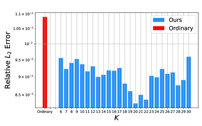
Figure 1: The relative error for each $K$ from 6 to 30. The y-axis is the relative $L_{2}$ error; the x-axis is the value of $K$.

$K$ is one of the most important hyperparameters in our framework. We investigate how the relative error varies depending on the value of $K$. We vary the value of $K$, recording the corresponding errors in Figure 1. As illustrated in Figure 1, our framework performs best when $K=20$. Around $K=20$, it is experimentally confirmed that the performance worsens if $K$ increases or decreases.

This result can be interpreted from the perspective of the receptive field. Before addressing that point, we note that the derivative is a kind of local property. The derivative of a function at a query point depends only on its local neighborhoods, and $K$ determines the range of such neighborhoods. Thus, the choice of $K$ can be regarded as adjusting the range of the receptive field for calculating the derivatives. Consequently, it is natural that a moderate, neither too large nor too small, value for $K$ is most suitable.

4.2.3 Hyperparameter Selection for the order of polynomial

Table 3: The relative error for Darcy2d-dataset corresponding to the order of the polynomial $p(x)$, ranging from 1 to 4.

$m$	1	2	3	4
Errors	9.21e-03	8.25e-03	9.33e-03	3.30e-02

We next conduct an ablation study for $m$, the order of $p(x)$ defined by Equation 2, to choose the most suitable value. We systematically vary the value of $m$ from 1 to 4 for Sobolev Training, recording the corresponding errors in Table 3. As described in Table 3, we observe that the case of $m=2$ has the best performance. We also observe a sharp decline in performance when $m=4$, as an order that is too high, increases learning complexity, resulting in training difficulties.

4.2.4 Ablation Studies for the regularity conditions

One of the most important conditions in our framework is the regularity condition, specifically $u\in W^{M,2}(\Omega)$. We investigate the influence of the regularity condition on performance by intentionally omitting it.

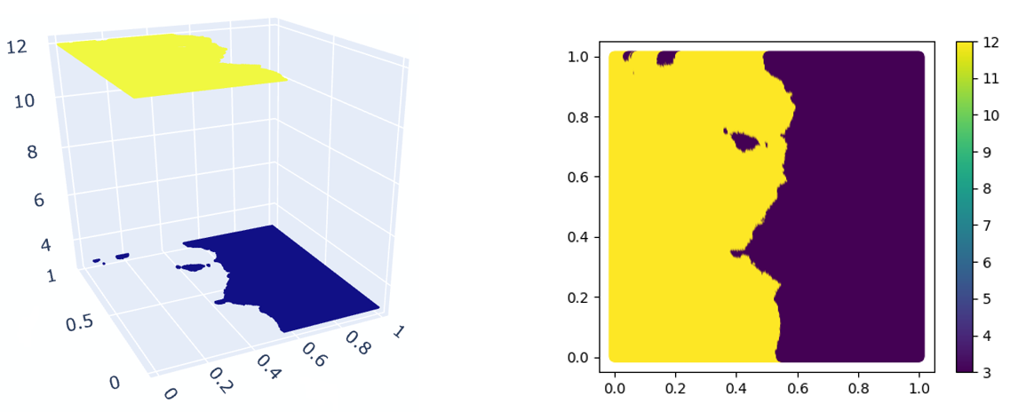
Figure 2: Visualization of coefficient function $a$ of the Darcy2d-dataset. Due to jump discontinuity, $a\in L^{\infty}((0,1)^{2};\mathbb{R}_{+})$ fails to belong to $W^{M,2}((0,1)^{2})$ for all $M\in\mathbb{N}$.

Table 4: Relative errors for the inverse problem of Darcy2d. We compare three training types: ours and the ordinary training (with/without) Finite Difference Methods.

Training Type	Error
Ours	4.78e-02
Ordinary	2.47e-02
Ordinary + FDM	6.93e-02

Here, we address the inverse problem of Darcy2d, aiming to learn a mapping from the solution $u$ to the coefficient $a$. Unlike the forward problem, the target $a\in L^{\infty}((0,1)^{2};\mathbb{R}_{+})$ does not belongs to $W^{M,2}((0,1)^{2})$ for any $M\in\mathbb{N}$ (see Figure 2).

We conduct the experiments for the Galerkin Transformer, which performs best on the inverse problem of Darcy2d among baselines. The comparisons involve our approach and the ordinary training, both with and without FDM. As described in Table 4, our ordinary training with FDM performs worse than the ordinary one. This is interpreted as a result of the absence of regularity conditions for the target function $a$. Since $a$ is not differentiable due to jump discontinuity, applying Sobolev Training in this case is unsuccessful. This experiment confirms that the regularity condition is necessary to apply Sobolev Training successfully.

4.2.5 Ablation Studies for PCGrad

Table 5: Comparison of relative errors on Darcy2d dataset when applying and not applying PCGrad.
With PCGrad : Sobolev Training with applying PCGrad
Without PCGrad : Sobolev Training optimizing Equation 11 directly rather than applying PCGrad

Training Type	Error
with PCGrad	7.34e-03
without PCGrad	8.01e-03
Ordinary	8.40e-03

Our last experiment is to evaluate the impact of applying PCGrad to Sobolev Training on performance. As aforementioned in Section 3.3, we conduct an ablation study for PCGrad to confirm the effectiveness of PCGrad experimentally. We estimate the relative error on the Darcy2d dataset using the Galerkin Transformer, comparing the cases of applying and not applying PCGrad, i.e., directly optimizing Equation 11. The results are described in Table 5. According to Table 5, the error consistently decreases compared to the ordinary case when Sobolev Training, and particularly, it is confirmed that the performance is further enhanced when combined with PCGrad compared to when not using it.

5 Conclusion

In this study, we explore the impact of Sobolev Training on operator learning. Theoretically, we demonstrate that, in the case of a one-layer ReLU network with several assumptions on the kernel function, incorporating a derivative term accelerates the convergence rate. Our numerical experiments further reveal that Sobolev Training significantly influences a variety of datasets and models. Our future work aims to extend these theoretical findings to more general cases and refine the proposed derivative approximation algorithm. This direction promises to enhance the robustness and applicability of our approach in the field of operator learning.

Appendix A Notations

Let us revisit some of the notations mentioned in Section 2.1 and introduce additional notations to explain details on the algorithm and the theorem proposed in Section 3.

• For $m_{1},m_{2}\in\mathbb{Z}$, we use the notation $[m_{1},\cdots,m_{2}]$ to denote an array of integers from $m_{1}$ to $m_{2}$.

• $\alpha=(\alpha^{1},\cdots,\alpha^{n})\in\left(\mathbb{N}\cup\{0\}\right)^{n}$ denotes a multi-index.

• We use the notation $|\alpha|=\sum_{i=1}^{n}\alpha^{i}$ and $\alpha!=(\alpha^{1})!(\alpha^{2})!\cdots(\alpha^{n})!$.

• $D_{x}^{\alpha}$ represents a derivative in the $x$ direction of order $\alpha$.

• We denote $D_{x}u=(\partial_{1}u,\cdots,\partial_{n}u)$, where each $\partial_{i}u$ denotes the partial derivative of $u$ with respect to the $i^{th}$ variable.

• We use $w\in\mathbb{R}^{n}$ to denote the weight of the neural network, and $D_{w}u(x;w)$ represents the derivative of $u$ with respect to the weight $w$.

• For $x\in\mathbb{R}^{n}$, we denote $x=(x^{1},x^{2},\cdots,x^{n})$ and $\|x\|=\sqrt{(x^{1})^{2}+\cdots+(x^{n})^{2}}$.

• We use the notation $f\stackrel{{\scriptstyle\gamma}}{{\approx}}g$, if there a universal constant $C=C(\gamma)>1$ such that

  $$\frac{1}{C}g\leq f\leq Cg.$$

• For a bounded domain $\Omega\subset\mathbb{R}^{n}$, we denote

  $$|\Omega|=\int_{\Omega}dx.$$

Appendix B Details of Algorithm 1

This section offers a more detailed explanation of the derivative approximation algorithm. For instance, when $n=2$ and $m=2$, we consider the two-dimensional case where the degree of the approximating polynomial is less than or equal to $2$. We denote $x=(x^{1},x^{2})$ and mesh points are denoted as $x_{j}=(x_{j}^{1},x_{j}^{2})$. The basis vector of $\Pi_{2}^{2}$ is

$$b_{j}(x)=\begin{pmatrix}1\\ x^{1}-x_{j}^{1}\\ x^{2}-x_{j}^{2}\\ (x^{1}-x_{j}^{1})^{2}\\ (x^{1}-x_{j}^{1})(x^{2}-x_{j}^{2})\\ (x^{2}-x_{j}^{2})^{2}\end{pmatrix}.$$

For each $x_{j}\in\{x_{j}\}_{j=1}^{J}$, we find K nearest points $\{x_{KNN,j,1},\cdots,x_{KNN,j,K}\}\subset\{x_{j}\}_{j=1}^{J}$ and calculate the coefficient vector $c_{j}$ using Equation 3 with

$$\omega(t)=\left(1-\frac{t}{D}\right)^{4}\left(\frac{4t}{D}+1\right)\quad\text{and }\quad D=1.1*\max_{j,k}\|x_{j}-x_{KNN,j,k}\|.$$ (15)

Since the average time complexity of widely used KNN algorithms (KD-tree, Ball-Tree) is $O(\log N)$ and matrix inversion has a time complexity of $O(K^{3})$ for $K\times K$ matrix, Algorithm 1 has an average time complexity of $O(K^{4}N\log N)$. Since $K$ is very small compared to $N$ and fixed number, the time complexity of Algorithm 1 is $O(N\log N)$ considering $K$ as a constant.

Appendix C Proof of theorems in Section 3

This section provides detailed proof of theorems in Section 3.

C.1 Proof of Lemma 3.1

Proof.

Let us assume $u\in C^{M}(\Omega)$ for some $M\in\mathbb{N}$. We define the matrices $W_{j}\in\mathbb{R}^{K\times K}$ and $E_{j}\in\mathbb{R}^{K\times I}$ as follows:

$$W_{j} =\text{diag}(\omega_{j,1},\ldots,\omega_{j,K})\quad\text{where}\quad\omega_{j,k}=\omega(|x_{j}-x_{j,\text{KNN},k}|),$$

$$E_{kj} =b_{j}(x_{j,\text{KNN},k})\quad\text{for}\quad k\in[1,\ldots,K],\ j\in[1,\ldots,J].$$

Further, we define $A_{j}:=E_{j}^{T}W_{j}E_{j}$ and $A_{j,\tilde{j}\xleftarrow{}w}$ to be the matrix formed by replacing the $\tilde{j}^{th}$ column of $A_{j}$ with the vector $w$.

Now, for each $j\in[1,J]$ and a multi-index $\alpha_{\tilde{j}}$ with $|\alpha_{\tilde{j}}|=m$, we apply Theorem 3.1 of (Lipman et al., 2006) to obtain

$$c_{j,\alpha_{\tilde{j}}}-D_{x}^{\alpha_{\tilde{j}}}u(x_{j})=\sum_{|\alpha|=M}\sum_{k=1}^{K}\frac{1}{\alpha!}D^{\alpha}_{x}u(x_{j}+\theta_{j,k}(x_{j}-x_{KNN,j,k}))|x_{j}-x_{KNN,j,k}|^{\alpha}\frac{\det(A_{j,\tilde{j}\xleftarrow{}w_{k}b_{j}(x_{k})})}{\det(A_{j})}$$ (16)

for some $0\leq\theta_{KNN,j,k}\leq 1$. We denote $s=\sum_{\tilde{j}=1}^{I}|\alpha_{\tilde{j}}|$ and use Remark 4 of (Liang & Zhao, 2013) to have

$$\det(A_{j,\tilde{j}\xleftarrow{}w_{k}b_{i}(x_{k})})\approx O(h^{2s-|\alpha_{\tilde{j}}|})\quad\text{and}\quad\det(A)\approx O(h^{2s}).$$

From the relations above, it is directly checked that

$$\frac{\det(A_{j,\tilde{j}\xleftarrow{}w_{k}b_{j}(x_{k})})}{\det(A_{j})}\leq Ch^{-|\alpha_{\tilde{j}}|}.$$

First, take a square on the both side of Equation 16, then take average over $j=1\cdots J$ and take summation for all multi-index satisfying $|\alpha_{\tilde{j}}|=m$, finally then use assumption Equation 4 to conclude

$$\frac{1}{J}\sum_{|\alpha_{\tilde{j}}|=m}\sum_{j=1}^{J}|c_{j,\alpha_{\tilde{j}}}-D^{\alpha_{\tilde{j}}}_{x}u(x_{j})|^{2} \leq Ch^{M-m}\|u\|_{W^{M,2}(\Omega)}.$$

Then the proof is complete by approximating $u\in W^{M,2}(\Omega)$ by $C^{M}(\Omega)$ function using Theorem 5.3.2 of (Evans, 2022). ∎

C.2 Proof of Theorem 3.2

We need the following auxiliary lemmas to prove the main theorem of this paper. One can achieve the result from a direct computation.

Lemma C.1.

Suppose that

$$A\in\mathbb{R}^{1\times d},\quad B\in\mathbb{R}^{J\times d}\quad\text{and}\quad w\in\mathbb{R}^{d\times 1}.$$

If $f(w):=AwBw$, then we establish

$$D_{w}f(w)=AwB+BwA.$$

The proof of the following lemma can be found in Section 15.10 in (Ord & Stuart, 1994).

Lemma C.2.

Suppose that

$$x,y\sim\mathcal{N}(0,1)$$

with a correlation $\rho\in[0,1]$. Then we denonstrate

$$\mathbb{P}\left[x>0,y>0\right]=\frac{1}{4}+\frac{1}{2\pi}\arcsin{\rho}$$

Let us denote $\theta(w_{1},w_{2})\in[0,\pi]$ by the angle between $w_{1}$ and $w_{2}\in\mathbb{R}^{n}$ . For the notational convenience, we denote

$$C(e,w) =\frac{1}{2\pi}[(\pi-\theta(e,w))w+\|w\|\sin\theta(e,w)e]\in\mathbb{R}^{d\times 1},$$

$$\alpha(w_{1},w_{2}) =w_{1}^{T}C\left(\frac{w_{1}}{\|w_{1}\|},w_{2}\right)=\frac{\|w_{1}\|\|w_{2}\|}{2\pi}[(\pi-\theta(w_{1},w_{2}))\cos\theta(w_{1},w_{2})+\sin\theta(w_{1},w_{2})]\in\mathbb{R}.$$

Furthermore, we denote

$$\phi_{0}(w_{1},w_{2}) =\frac{1}{2\pi}[(\pi-\theta(w_{1},w_{2}))\cos\theta(w_{1},w_{2})+\sin\theta(w_{1},w_{2})]$$

$$\phi_{1}(e,w) =\frac{1}{2\pi}(\pi-\theta(e,w))$$

$$\phi_{2}(e,w) =\frac{1}{2\pi}\sin\theta(e,w).$$

Note that one can directly check that

$$C(e,w)=\phi_{1}(e,w)w+\phi_{2}(e,w)\|w\|e\quad\text{and}\quad\alpha(w_{1},w_{2})=\|w_{1}\|\|w_{2}\|\phi_{0}(w_{1},w_{2}).$$

We need the following results from Theorem 1 of (Tian, 2017).

Lemma C.3.

Let us denote

$$F(X,e,w):=X^{T}D(X,e)D(X,w)Xw.$$ (17)

Then we find

$$\mathbb{E}_{X}\left[F(X,e,w)\right]=\frac{J}{2\pi}[(\pi-\theta(e,w))w+\|w\|\sin\theta(e,w)e]=JC(e,w).$$

Lemma C.4.

Let us define

$$g(\theta):=(\cos\theta-1)((\pi-\theta)(\cos\theta-1)+2\sin\theta).$$

Then $g(\theta)\leq 0$ for all $\theta\in[0,\pi]$.

Proof.

Cleary, we observe that $g(0)=g(\pi)=0$. Also, from a direct computation, we find

$$g^{\prime}(\theta)=\sin\theta(-3\sin\theta+2(\pi-\theta)(1-\cos\theta)).$$

If $g^{\prime}(\theta_{0})=0$ and $0<\theta_{0}<\pi$, then $\sin\theta_{0}\not=0$ and we have

$$3\sin\theta_{0}=2(\pi-\theta_{0})(1-\cos\theta_{0}).$$ (18)

By Equation 18 and some mathematical manipulation, we find

$$g(\theta_{0})=\frac{\pi-\theta_{0}}{3}(\cos\theta_{0}-1)(1-\cos\theta_{0})<0.$$

The strict inequality holds because $\cos\theta_{0}\not=0$. Taking twice derivative of $g(\theta)$, we find

$$g^{\prime\prime}(\theta)=-2((\theta-\pi)(2\cos^{2}\theta-\cos\theta-1)+\sin\theta(1+2\cos\theta)).$$

By Equation 18 again, we find

$$g^{\prime\prime}(\theta_{0}) =-2\left((\pi-\theta_{0})(2\cos^{2}\theta_{0}-\cos\theta_{0}-1)+\frac{2}{3}(\pi-\theta_{0})(1-\cos\theta_{0})(2\cos\theta_{0}+1)\right)$$

$$=-\frac{2}{3}(\pi-\theta_{0})(2\cos^{2}\theta_{0}-\cos\theta_{0}-1)$$

$$=-\frac{2}{3}(\pi-\theta_{0})(2\cos\theta_{0}+1)(\cos\theta_{0}-1).$$

Note that if $0<\theta_{0}<\frac{5\pi}{6}$, then $-\frac{1}{2}\leq\cos\theta_{0}\leq 1$, which implies that $g^{\prime\prime}(\theta_{0})>0$, as $(2t+1)(t-1)<0$ for $-\frac{1}{2}<t<1$. On the other hand, if $\frac{5\pi}{6}\leq\theta_{0}<\pi$, then we have

$$g^{\prime}(\theta_{0})=\sin\theta_{0}(\pi-\theta_{0})(1-\cos\theta)\left(2-\frac{3\sin\theta_{0}}{(\pi-\theta_{0})(1-\cos\theta_{0})}\right).$$

Reminding $\sin\theta>\theta$ for all $\theta>0$, it is evident that

$$\frac{\sin\theta_{0}}{\pi-\theta_{0}}=\frac{\sin(\pi-\theta_{0})}{\pi-\theta_{0}}<1\quad\text{and}\quad\frac{3}{2}\leq 1-\cos\theta_{0}\leq 2,$$

to get $g^{\prime}(\theta_{0})>0$. These calculations imply that $\theta_{0}$ is not the extreme point. Therefore, all the extreme points are local minimums, implying that there exists only one local minimum of $g(\theta)$ at $\theta_{0}\in(0,\pi)$ and $g(\theta_{0})<0$. We can finally conclude that $g(\theta)\leq 0$ for all $0\leq\theta\leq\pi$. ∎

The following lemma can be directly from elementary calculation.

Lemma C.5.

Let us define a real-valued 3rd-order polynomial

$$f(t):=At^{3}-Bt^{2}-Ct+D.$$

If $A>0$ and $B^{2}+3AC>0$, then $f(t)$ has a local minimum at

$$t_{0}=\frac{B+\sqrt{B^{2}+3AC}}{3A},$$

and the value of the local minimum value is

$$f(t_{0})=\frac{1}{27A^{2}}\left(27A^{2}D-2B^{3}-9ABC-2(B^{2}+3AC)\sqrt{B^{2}+3AC}\right).$$

Proof of Theorem 3.2

Proof.

In this work, we consider a real-valued function; that is, we assume that

$$x\in\mathbb{R}^{d}\quad\text{and}\quad u(x),v(x)\in\mathbb{R}.$$

Consider the sets of input and output function pairs, denoted by $\{u_{k}(x),v_{k}(x)\}_{k=1}^{N}$. Additionally, let $\{x_{j}\}_{j=1}^{J}$ and $\{y_{l}\}_{l=1}^{\tilde{J}}$ represent query points that are sampled from a spherical Gaussian distribution $\mathcal{N}(0,I)$. We also assume that $x_{j}$ and $y_{l}$ are independently sampled for all $j$ and $l$. Let $X=[x_{1},x_{2},\cdots,x_{J}]\in\mathbb{R}^{J\times n}$ and $Y=[y_{1},y_{2},\cdots,y_{\tilde{J}}]\in\mathbb{R}^{\tilde{J}\times n}$ be a matrix representation of each query points. We represent each $u_{k}$ using a Monte Carlo approximation, as in

$$u_{k}(x_{j})=\frac{1}{|\Omega|}\int_{\Omega}\kappa(x_{j},y)v_{k}(y)d\nu(y)\approx\frac{1}{\tilde{J}}\sum_{l=1}^{\tilde{J}}\mathbb{E}_{Y}\left[\kappa(x_{j},y_{l})v_{k}(y_{l})\right].$$ (19)

As explained in Section 3, we assume $v_{k}(y_{l})$ and $\kappa(x,y)$ can be expressed as is given as

$$v_{k}(x)=\mu_{k}\sigma((w^{*})^{T}x)\quad\text{and}\quad\kappa(x,y)=\sigma(w^{T}x)\sigma(w^{T}y).$$ (20)

Using the matrix representation Equation 19, assumption Equation 20 and Lemma C.3, we have

$$u_{k}(X;w) =\frac{\mu_{k}(w^{*})^{T}}{\tilde{J}}\mathbb{E}_{Y}\left[Y^{T}D(Y,w^{*})D(Y,w)Yw\right]D(X,w)Xw$$ (21)

$$=\frac{\mu_{k}(w^{*})^{T}}{\tilde{J}}\mathbb{E}_{Y}\left[F\left(Y,\frac{w^{*}}{\|w^{*}\|},w\right)\right]D(X,w)Xw$$

$$=\frac{\mu_{k}(w^{*})^{T}}{2\pi}\left[(\pi-\theta(w,w^{*}))w+\|w\|\sin\theta(w,w^{*})\frac{w^{*}}{\|w^{*}\|}\right]D(X,w)Xw$$

$$=\mu_{k}(w^{*})^{T}C\left(\frac{w^{*}}{\|w^{*}\|},w\right)D(X,w)Xw$$

$$=\mu_{k}\alpha(w,w^{*})D(X,w)Xw.$$

Applying Lemma C.1 to $u_{k}(X;w)$, we find

$$D_{w}u_{k}(X;w) =\mu_{k}\alpha(w,w^{*})D(X,w)X+\frac{\mu_{k}}{\tilde{J}}D(X,w)Xw\mathbb{E}_{Y}\left[(w^{*})^{T}Y^{T}D(Y,w^{*})D(Y,w)Y\right].$$ (22)

For $w_{1},w_{2}\in\mathbb{R}^{d}$, one use Equations 21, 22 and 17 and Lemma C.3 to have

$$\left[D_{w}u_{k}(X;w_{2})\right]^{T}u_{k}(X;w_{1})$$

$$=|\mu_{k}|^{2}\alpha(w^{*},w_{1})\alpha(w^{*},w_{2})X^{T}D(X,w_{2})D(X,w_{1})Xw_{1}$$

$$\quad+\frac{\mu_{k}^{2}\alpha(w^{*},w_{1})}{\tilde{J}}\mathbb{E}_{Y}\left[Y^{T}D(Y,w_{2})D(Y,w^{*})Yw^{*}\right]w_{2}^{T}X^{T}D(W,w_{2})D(X,w_{1})Xw_{1}$$

$$=|\mu_{k}|^{2}\alpha(w^{*},w_{1})\alpha(w^{*},w_{2})F\left(X,\frac{w_{2}}{\|w_{2}\|},w_{1}\right)+\frac{|\mu_{k}|^{2}\alpha(w^{*},w_{1})}{\tilde{J}}E_{Y}[F\left(Y,\frac{w_{2}}{\|w_{2}\|},w^{*}\right)]w_{2}^{T}F\left(X,\frac{w_{2}}{\|w_{2}\|},w_{1}\right)$$

$$=|\mu_{k}|^{2}\alpha(w^{*},w_{1})\alpha(w^{*},w_{2})F\left(X,\frac{w_{2}}{\|w_{2}\|},w_{1}\right)+|\mu_{k}|^{2}\alpha(w^{*},w_{1})C\left(\frac{w_{2}}{\|w_{2}\|},w^{*}\right)w_{2}^{T}F\left(X,\frac{w_{2}}{\|w_{2}\|},w_{1}\right)$$

$$=|\mu_{k}|^{2}\left(\alpha(w_{2},w^{*})I_{d}+C\left(\frac{w_{2}}{\|w_{2}\|},w^{*}\right)w_{2}^{T}\right)\alpha(w^{*},w_{1})F\left(X,\frac{w_{2}}{\|w_{2}\|},w_{1}\right).$$

This leads to

$$\left[D_{w}u_{k}(X;w)\right]^{T}\left(u_{k}(X;w)-u_{k}(X;w^{*})\right)$$

$$=|\mu_{k}|^{2}\left(\alpha(w,w^{*})I_{d}+C\left(\frac{w}{\|w\|},w^{*}\right)w^{T}\right)\left(\alpha(w,w^{*})F\left(X,\frac{w}{\|w\|},w\right)-\alpha(w^{*},w^{*})F\left(X,\frac{w}{\|w\|},w^{*}\right)\right).$$

Therefore, it follows that

$$\mathbb{E}_{X}\left[\frac{\partial\mathcal{L}_{L^{2}}}{\partial w}\right]=\frac{1}{NJ}\sum_{k=1}^{N}\left[D_{w}u_{k}(X;w)\right]^{T}\left(u_{k}(X;w)-u_{k}(X;w^{*})\right),$$

where $\mathcal{L}_{L^{2}}$ is the loss function defined as in Equation 9. If $w$ is updated by $\lx@cref{creftype~refnum}{eq:gradient_flow}_{1}$, it is directly checked that

$$\frac{1}{2}\frac{d}{dt}\|w-w^{*}\|^{2}$$

$$=(w-w^{*})^{T}\frac{dw}{dt}$$

$$=-(w-w^{*})^{T}\mathbb{E}_{X}\left[\frac{\partial\mathcal{L}_{L^{2}}}{\partial w}\right]$$

$$=-\frac{1}{NJ}\sum_{k=1}^{N}|\mu_{k}|^{2}(w-w^{*})^{T}\left(\alpha(w,w^{*})I_{d}+C\left(\frac{w}{\|w\|},w^{*}\right)w^{T}\right)$$

$$\quad\times\left(\alpha(w,w^{*})\mathbb{E}_{X}\left[F\left(X,\frac{w}{\|w\|},w\right)\right]-\alpha(w^{*},w^{*})\mathbb{E}_{X}\left[F\left(X,\frac{w}{\|w\|},w^{*}\right)\right]\right)$$

$$=-\frac{1}{N}\sum_{k=1}^{N}|\mu_{k}|^{2}(w-w^{*})^{T}\left(\alpha(w,w^{*})I_{d}+C\left(\frac{w}{\|w\|},w^{*}\right)w^{T}\right)$$

$$\quad\times\left(\alpha(w,w^{*})C\left(\frac{w}{\|w\|},w\right)-\alpha(w^{*},w^{*})C\left(\frac{w}{\|w\|},w^{*}\right)\right).$$

For each $k=1\cdots N$, it follows that

$$(w-w^{*})^{T}\left(\alpha(w,w^{*})I_{d}+C\left(\frac{w}{\|w\|},w^{*}\right)w^{T}\right)$$

$$=(w-w^{*})^{T}\left(\|w\|\|w^{*}\|\phi_{0}(w,w^{*})+\phi_{1}(w,w^{*})w^{*}w^{T}+\phi_{2}(w,w^{*})\frac{\|w^{*}\|}{\|w\|}ww^{T}\right)$$

$$=\|w\|\|w^{*}\|\phi_{0}(w,w^{*})(w-w^{*})^{T}+\phi_{1}(w,w^{*})w^{T}w^{*}w^{T}+\phi_{2}(w,w^{*})\|w^{*}\|\|w\|w^{T}$$

$$\quad-\phi_{1}(w,w^{*})(w^{*})^{T}w^{*}w^{T}-\phi_{2}(w,w^{*})\frac{\|w^{*}\|}{\|w\|}(w^{*})^{T}ww^{T}$$

$$=\|w\|\|w^{*}\|\phi_{0}(w,w^{*})(w-w^{*})^{T}+\phi_{0}(w,w^{*})\|w^{*}\|\|w\|w^{T}$$

$$\quad-\phi_{1}(w,w^{*})\|w^{*}\|^{2}w^{T}-\phi_{2}(w,w^{*})\|w^{*}\|^{2}\cos\theta(w,w^{*})w^{T}$$

$$=2\|w\|\|w^{*}\|\phi_{0}(w,w^{*})w^{T}-\|w\|\|w^{*}\|\phi_{0}(w,w^{*})(w^{*})^{T}$$

$$\quad-\|w^{*}\|^{2}\phi_{1}(w,w^{*})w^{T}-\|w^{*}\|^{2}\phi_{2}(w,w^{*})\cos\theta(w,w^{*})w^{T}$$

$$=:I_{1}+I_{2}+I_{3}+I_{4}.$$

Next, we calculate

$$\alpha(w,w^{*})C\left(\frac{w}{\|w\|},w\right)-\alpha(w^{*},w^{*})C\left(\frac{w}{\|w\|},w^{*}\right)$$

$$=\|w^{*}\|\|w\|\phi_{0}(w,w^{*})\left(\phi_{1}(w,w)w+\phi_{2}(w,w)w\right)$$

$$\quad-\|w^{*}\|\|w^{*}\|\phi_{0}(w^{*},w^{*})\left(\phi_{1}(w,w^{*})w^{*}+\phi_{2}(w,w^{*})\frac{\|w^{*}\|}{\|w\|}w\right)$$

$$=\frac{1}{2}\|w^{*}\|\|w\|\phi_{0}(w,w^{*})w-\frac{1}{2}\|w^{*}\|^{2}\phi_{1}(w,w^{*})w^{*}$$

$$\quad-\frac{1}{2}\frac{\|w^{*}\|^{3}}{\|w\|}\phi_{2}(w,w^{*})w$$

$$=:J_{1}+J_{2}+J_{3}.$$

Note that we have used the fact that $\phi_{1}(w,w)=\frac{1}{2}$ and $\phi_{2}(w,w)=0$. From a direct computation, it follows that

$$I_{1}J_{1} =\|w\|^{4}\|w^{*}\|^{2}\phi_{0}(w,w^{*})^{2},$$

$$I_{2}J_{1} =-\frac{1}{2}\|w\|^{3}\|w^{*}\|^{3}\phi_{0}(w,w^{*})^{2}\cos\theta(w,w^{*}),$$

$$I_{3}J_{1} =-\frac{1}{2}\|w\|^{3}\|w^{*}\|^{3}\phi_{0}(w,w^{*})\phi_{1}(w,w^{*}),$$

$$I_{4}J_{1} =-\frac{1}{2}\|w\|^{3}\|w^{*}\|^{3}\phi_{0}(w,w^{*})\phi_{2}(w,w^{*})\cos\theta(w,w^{*}),$$

$$I_{1}J_{2} =-\|w\|^{2}\|w^{*}\|^{4}\phi_{0}(w,w^{*})\phi_{1}(w,w^{*})\cos\theta(w,w^{*}),$$

$$I_{2}J_{2} =\frac{1}{2}\|w\|\|w^{*}\|^{5}\phi_{0}(w,w^{*})\phi_{1}(w,w^{*}),$$

$$I_{3}J_{2} =\frac{1}{2}\|w\|\|w^{*}\|^{5}\phi_{1}(w,w^{*})^{2}\cos\theta(w,w^{*}),$$

$$I_{4}J_{2} =\frac{1}{2}\|w\|\|w^{*}\|^{5}\phi_{1}(w^{*},w^{*})\phi_{2}(w,w^{*})\cos^{2}\theta(w,w^{*}),$$

$$I_{1}J_{3} =-\|w\|^{2}\|w^{*}\|^{4}\phi_{0}(w,w^{*})\phi_{2}(w^{*},w^{*}),$$

$$I_{2}J_{3} =\frac{1}{2}\|w\|\|w^{*}\|^{5}\phi_{0}(w^{*},w^{*})\phi_{0}(w,w^{*})\phi_{2}(w,w^{*})\cos\theta(w,w^{*}),$$

$$I_{3}J_{3} =\frac{1}{2}\|w\|\|w^{*}\|^{5}\phi_{1}(w^{*},w^{*})\phi_{2}(w,w^{*}),$$

$$I_{4}J_{3} =\frac{1}{2}\|w\|\|w^{*}\|^{5}\phi_{2}(w^{*},w^{*})^{2}\cos\theta(w^{*},w^{*}).$$

Taking the summation over $I_{i}J_{j}$ for $i\in\{1,2,3\}$ and $j\in\{1,2,3,4\}$, we arrive at

$$\frac{1}{2}\frac{d}{dt}\|w-w^{*}\|^{2} =-\frac{1}{N}\sum_{k=1}^{N}|\mu_{k}|^{2}\|w\|\|w^{*}\|^{5}\left(M_{3}\left(\frac{\|w\|}{\|w^{*}\|}\right)^{3}-M_{2}\left(\frac{\|w\|}{\|w^{*}\|}\right)^{2}-M_{1}\left(\frac{\|w\|}{\|w^{*}\|}\right)+M_{0}\right),$$

where

$$M_{3} =\phi_{0}(w,w^{*})^{2},$$

$$M_{2} =\frac{1}{2}\phi_{0}(w,w^{*})\Big{[}\phi_{0}(w,w^{*})\cos\theta(w,w^{*})+\phi_{1}(w,w^{*})+\phi_{2}(w,w^{*})\cos\theta(w,w^{*})\Big{]},$$

$$M_{1} =\phi_{0}(w,w^{*})^{2},$$

$$M_{0} =\phi_{0}(w,w^{*})^{2}.$$

Then we arrive

$$\frac{1}{2}\frac{d}{dt}\|w-w^{*}\|^{2}$$ (23)

$$=-\frac{1}{N}\sum_{k=1}^{N}|\mu_{k}|^{2}\phi_{0}(w,w^{*})^{2}\|w\|\|w^{*}\|^{5}\left(\left(\frac{\|w\|}{\|w^{*}\|}\right)^{3}-\left(\frac{\|w\|}{\|w^{*}\|}\right)^{2}-\left(\frac{\|w\|}{\|w^{*}\|}\right)+1.\right)$$

$$\quad+\frac{1}{N}\sum_{k=1}^{N}\frac{|\mu_{k}|^{2}}{2}\|w\|^{3}\|w^{*}\|^{3}\phi_{0}(w,w^{*})\Big{[}(\cos\theta(w,w^{*})-2)\phi_{0}(w,w^{*})+\phi_{1}(w,w^{*})+\phi_{2}(w,w^{*})\cos\theta(w,w^{*})\Big{]}$$

$$=:K_{1}+K_{2}.$$

It is directly checked that $t^{3}-t^{2}-t+1\geq 0\quad\text{for all }t\geq 0$ which implies that $K_{1}\leq 0$. By denoting $\theta=\theta(w,w^{*})$ , we compute

$$(\cos\theta-2)\phi_{0}(w,w^{*})+\phi_{1}(w,w^{*})+\phi_{2}(w,w^{*})\cos\theta(w,w^{*})$$

$$=((\pi-\theta)\cos\theta+\sin\theta)(\cos\theta-2)+(\pi-\theta)+\sin\theta\cos\theta$$

$$=(\cos\theta-1)((\pi-\theta)(\cos\theta-1)+2\sin\theta)=:g(\theta).$$

By Lemma C.4, we have $g(\theta)\leq 0$ for all $\theta\in[0,\pi]$ implying that $K_{2}\leq 0$. Note that

$$\frac{1}{2}\frac{d}{dt}\|w-w^{*}\|^{2}=0\iff K_{1}=K_{2}=0.$$

This equality holds only when $\|w\|=\|w^{*}\|$ and $\theta(w,w^{*})=0$ or $\pi$. If $\theta(w,w^{*})=0$, then $w=w^{*}$. On the other hand, if $\theta(w,w^{*})=\pi$ and $\|w\|=\|w^{*}\|$, then $w=-w^{*}$ and $w\not\in\{\|w-w^{*}\|<\|w^{*}\|\}$. Therefore, we have

$$\frac{d}{dt}\|w-w^{*}\|^{2}<0\quad\text{under the assumption }w_{0}\in\{\|w-w^{*}\|<\|w^{*}\|\}.$$

Moreover, from the fact that $\frac{1}{2}\|w-w^{*}\|^{2}\leq\frac{1}{2}\|w^{*}\|^{2}$, once $w_{0}\in\{\|w-w^{*}\|<\|w^{*}\|\}$, the parameter vector $w$ remains in $\{\|w-w^{*}\|<\|w^{*}\|\}$, thus $w\to w^{*}$ as $t\to\infty$.

Let us show that adding derivative information to the loss function enhances convergence speed. Representation Equation 21 using a vector $x\in\mathbb{R}^{n}$ instead of the matrix $X\in\mathbb{R}^{J\times n}$ then taking derivative in $x$ variable, we have

$$D_{x}u_{k}(x;w) =D_{x}\left[\mu_{k}\alpha(w,w^{*})\mathbbm{1}_{\{x^{T}w>0\}}(x^{T}w)\right]$$

$$=\mu_{k}\alpha(w,w^{*})\mathbbm{1}_{\{x^{T}w>0\}}w.$$

Similarly, when using the vector representation of Equation 22, we find

$$D_{x}D_{w}u_{k}(x;w) =D_{x}\left[\mu_{k}\alpha(w,w^{*})\mathbbm{1}_{x^{T}w}x+\frac{\mu_{k}}{\tilde{J}}\mathbbm{1}_{\{x^{T}w>0\}}x^{T}w\mathbb{E}_{Y}\left[Y^{T}D(Y,w)D(Y,w^{*})Yw^{*}\right]\right]$$

$$=\mu_{k}\alpha(w,w^{*})\mathbbm{1}_{\{x^{T}w>0\}}I_{d}+\frac{\mu_{k}}{\tilde{J}}\mathbbm{1}_{\{x^{T}w>0\}}\mathbb{E}_{Y}\left[Y^{T}D(Y,w)D(Y,w^{*})Yw^{*}\right]w^{T}$$

$$=\mu_{k}\alpha(w,w^{*})\mathbbm{1}_{\{x^{T}w>0\}}I_{d}+\mu_{k}\mathbbm{1}_{\{x^{T}w>0\}}C\left(\frac{w}{\|w\|},w^{*}\right)w^{T}$$

Let $\mathcal{L}_{Der}$ be the loss function defined in equation Equation 10. We then compute

$$D_{w}\mathcal{L}_{Der}$$ (24)

$$=\frac{1}{JN}\sum_{k=1}^{N}\sum_{j=1}^{J}D_{w}D_{x}u_{k}(x_{j},w)^{T}(D_{x}u_{k}(x_{j},w)-D_{x}u_{k}(x_{j},w^{*}))$$

$$=\frac{1}{JN}\sum_{k=1}^{N}\sum_{j=1}^{J}|\mu_{k}|^{2}\left(\alpha(w,w^{*})\mathbbm{1}_{\{x_{j}^{T}w>0\}}I_{d}+\mathbbm{1}_{\{x_{j}^{T}w>0\}}w^{T}C\left(\frac{w}{\|w\|},w^{*}\right)^{T}\right)$$

$$\quad\times\left(\alpha(w,w^{*})\mathbbm{1}_{\{x_{j}^{T}w>0\}}w-\alpha(w^{*},w^{*})\mathbbm{1}_{\{x_{j}^{T}w^{*}>0\}}w^{*}\right)$$

$$=\frac{1}{JN}\sum_{k=1}^{N}\sum_{j=1}^{J}|\mu_{k}|^{2}\left(\alpha(w,w^{*})^{2}\mathbbm{1}_{\{x_{j}^{T}w>0\}}w+\alpha(w,w^{*})\mathbbm{1}_{\{x_{j}^{T}w>0\}}wC\left(\frac{w}{\|w\|},w^{*}\right)^{T}w\right.$$

$$\quad\left.-\alpha(w,w^{*})\alpha(w^{*},w^{*})\mathbbm{1}_{\{x_{j}^{T}w>0\}}\mathbbm{1}_{\{x_{j}^{T}w^{*}>0\}}w^{*}-\alpha(w,w^{*})\mathbbm{1}_{\{x_{j}^{T}w>0\}}\mathbbm{1}_{\{x_{j}^{T}w^{*}>0\}}wC\left(\frac{w}{\|w\|},w^{*}\right)^{T}w^{*}\right).$$

From the fact that $x_{j}\sim\mathcal{N}(0,I)$, we observe that $x_{j}^{T}w\sim\mathcal{N}(0,\|w\|^{2})$, $x_{j}^{T}w^{*}\in\mathcal{N}(0,\|w^{*}\|^{2})$, and the correlation between $x_{j}^{T}w$ and $x_{j}^{T}w^{*}$ is

$$\text{corr}(x_{j}^{T}w,x_{j}^{T}w^{*})=\frac{\mathbb{E}_{x_{j}}\left[(x_{j}^{T}w)(x_{j}^{T}w)\right]}{\mathbb{E}\left[(x_{j}^{T}w)^{2}\right]\mathbb{E}\left[(x_{j}^{T}w^{*})^{2}\right]}=\frac{w^{T}w^{*}}{\|w\|\|w^{*}\|}.$$

From these observations and Lemma C.2, it is directly checked that

$$\mathbb{E}_{x_{j}}\left[\mathbbm{1}_{\{x_{j}^{T}w>0\}}\right] =\mathbb{P}(x_{j}^{T}w>0)=\frac{1}{2},$$ (25)

$$\mathbb{E}_{x_{j}}\left[\mathbbm{1}_{\{x_{j}^{T}w>0\}}\mathbbm{1}_{\{x_{j}^{T}w^{*}>0\}}\right] =\mathbb{P}(x_{j}^{T}w>0,x_{j}^{T}w^{*}>0)=\frac{1}{4}+\frac{1}{2\pi}\arcsin\left({\frac{w^{T}w^{*}}{\|w\|\|w^{*}\|}}\right)$$

$$=\frac{1}{4}+\frac{1}{2\pi}\left(\frac{\pi}{2}-\theta(w,w^{*})\right)=\phi_{1}(w,w^{*}).$$

Let $w$ be the parameter vector following $\lx@cref{creftype~refnum}{eq:gradient_flow}_{2}$. Then it follows that

$$\frac{1}{2}\frac{d}{dt}\|w-w^{*}\|^{2}$$

$$=-(w-w^{*})^{T}\mathbb{E}_{X}\left[\frac{\partial\mathcal{L}_{Sob}}{\partial w}\right]$$

$$=-(w-w^{*})^{T}\mathbb{E}_{X}\left[\frac{\partial\mathcal{L}_{L^{2}}}{\partial w}\right]-(w-w^{*})^{T}\mathbb{E}_{X}\left[\frac{\partial\mathcal{L}_{Der}}{\partial w}\right]=:I_{1}+I_{2}.$$

To prove the effectiveness of Sobolev Training, we are left to show that $I_{2}\leq 0$. By Equations 24 and 25, we find

$$I_{2} =-\frac{1}{JN}\sum_{k=1}^{N}\sum_{j=1}^{J}|\mu_{k}|^{2}(w-w^{*})^{T}\Bigg{(}\alpha(w,w^{*})^{2}\mathbb{E}_{x_{j}}\left[\mathbbm{1}_{\{x_{j}^{T}w>0\}}\right]w$$

$$\quad+\alpha(w,w^{*})\mathbb{E}_{x_{j}}\left[\mathbbm{1}_{\{x_{j}^{T}w>0\}}\right]wC\left(\frac{w}{\|w\|},w^{*}\right)^{T}w$$

$$\quad-\alpha(w,w^{*})\alpha(w^{*},w^{*})\mathbb{E}_{x_{j}}\left[\mathbbm{1}_{\{x_{j}^{T}w>0\}}\mathbbm{1}_{\{x_{j}^{T}w^{*}>0\}}\right]w^{*}$$

$$\quad-\alpha(w,w^{*})\mathbb{E}_{x_{j}}\left[\mathbbm{1}_{\{x_{j}^{T}w>0\}}\mathbbm{1}_{\{x_{j}^{T}w^{*}>0\}}\right]wC\left(\frac{w}{\|w\|},w^{*}\right)^{T}w^{*}\Bigg{)}$$

$$=:-\frac{1}{JN}\sum_{k=1}^{N}\sum_{j=1}^{J}|\mu_{k}|^{2}(w-w^{*})^{T}I_{2k}$$

With help of Equation 25, we have

$$I_{2,k} =\frac{\alpha(w,w^{*})^{2}}{2}w+\frac{\alpha(w,w^{*})}{2}\left(\phi_{1}(w,w^{*})w^{*}+\phi_{2}(w,w^{*})\frac{\|w^{*}\|}{\|w\|}w\right)^{T}ww$$

$$\quad-\alpha(w,w^{*})\alpha(w^{*},w^{*})\phi_{1}(w,w^{*})w^{*}$$

$$\quad-\alpha(w,w^{*})\phi_{1}(w,w^{*})\left(\phi_{1}(w,w^{*})w^{*}+\phi_{2}(w,w^{*})\frac{\|w^{*}\|}{\|w\|}w\right)^{T}w^{*}w$$

$$=\frac{1}{2}\|w\|^{2}\|w^{*}\|^{2}\phi_{0}(w,w^{*})^{2}w$$

$$\quad+\frac{1}{2}\|w\|^{2}\|w^{*}\|^{2}\phi_{0}(w,w^{*})\left(\phi_{1}(w,w^{*})\cos\theta(w,w^{*})+\phi_{2}(w,w^{*})\right)w$$

$$\quad-\frac{1}{2}\|w^{*}\|^{3}\|w\|\phi_{0}(w,w^{*})\phi_{1}(w,w^{*})w^{*}$$

$$\quad-\|w^{*}\|^{3}\|w\|\phi_{0}(w,w^{*})\phi_{1}(w,w^{*})\left(\phi_{1}(w,w^{*})+\phi_{2}(w,w^{*})\cos\theta(w,w^{*})\right)w$$

$$=\|w\|^{2}\|w^{*}\|^{2}\phi_{0}(w,w^{*})^{2}w-\frac{1}{2}\|w^{*}\|^{3}\|w\|\phi_{0}(w,w^{*})\phi_{1}(w,w^{*})w^{*}$$

$$\quad-\|w^{*}\|^{3}\|w\|\phi_{0}(w,w^{*})\phi_{1}(w,w^{*})\left(\phi_{1}(w,w^{*})+\phi_{2}(w,w^{*})\cos\theta(w,w^{*})\right)w.$$

Then we calculate to have

$$(w-w^{*})I_{2,k}$$

$$=\|w\|^{4}\|w^{*}\|^{2}\phi_{0}(w,w^{*})^{2}$$

$$\quad-\|w\|^{3}\|w^{*}\|^{3}\phi_{0}(w,w^{*})^{2}\cos\theta(w,w^{*})$$

$$\quad-\frac{1}{2}\|w^{*}\|^{4}\|w\|^{2}\phi_{0}(w,w^{*})\phi_{1}(w,w^{*})\cos\theta(w,w^{*})$$

$$\quad+\frac{1}{2}\|w^{*}\|^{5}\|w\|\phi_{0}(w,w^{*})\phi_{1}(w,w^{*})$$

$$\quad-\|w^{*}\|^{3}\|w\|^{3}\phi_{0}(w,w^{*})\phi_{1}(w,w^{*})\left(\phi_{1}(w,w^{*})+\phi_{2}(w,w^{*})\cos\theta(w,w^{*})\right)$$

$$\quad+\|w^{*}\|^{4}\|w\|^{2}\phi_{0}(w,w^{*})\phi_{1}(w,w^{*})\cos\theta(w,w^{*})\left(\phi_{1}(w,w^{*})+\phi_{2}(w,w^{*})\cos\theta(w,w^{*})\right).$$

If $\phi_{0}(w,w^{*})\not=0$, we rearrange above equality as

$$\frac{(w-w^{*})^{T}I_{2,k}}{\phi_{0}(w,w^{*})\|w\|\|w^{*}\|^{5}} =M_{3}\left(\frac{\|w\|}{\|w^{*}\|}\right)^{3}-M_{2}\left(\frac{\|w\|}{\|w^{*}\|}\right)^{2}-M_{1}\left(\frac{\|w\|}{\|w^{*}\|}\right)+M_{0},$$ (26)

where

$$M_{3} =\phi_{0}(w,w^{*}),$$

$$M_{2} =\phi_{0}(w,w^{*})\cos\theta(w,w^{*})+\phi_{1}(w,w^{*})(\phi_{1}(w,w^{*})+\phi_{2}(w,w^{*})\cos\theta(w,w^{*})),$$

$$M_{1} =\phi_{1}(w,w^{*})\cos\theta(w,w^{*})\left(\frac{1}{2}-\phi_{1}(w,w^{*})-\phi_{2}(w,w^{*})\cos\theta(w,w^{*})\right),$$

$$M_{0} =\frac{1}{2}\phi_{1}(w,w^{*}).$$

For notational convenience, we denote

$$f(t)=M_{3}t^{2}-M_{2}t^{2}-M_{1}t+M_{0}.$$

Since $\phi_{0}(w,w^{*})\geq 0$, the signs of both sides of Equation 26 are the same. By Lemma C.5, $f(t)$ has a local minimum value at

$$t_{0}=\frac{M_{2}+\sqrt{M_{2}^{2}+3M_{1}M_{3}}}{3M_{3}},$$

with the value of

$$f(t_{0})=\frac{1}{27M_{3}^{2}}\left(27M_{3}^{2}M_{0}-2M_{2}^{3}-9M_{1}M_{2}M_{3}-2(M_{2}^{2}+3M_{1}M_{3})\sqrt{M_{2}^{2}+3M_{1}M_{3}}\right).$$

We may assume that $M_{3}^{2}+3M_{1}M_{3}\geq 0$. Otherwise, $f(t)$ is an increasing function, and since $f(0)=M_{0}\geq 0$, there is nothing to show. We are left to show that $f(t_{0})\geq 0$ if $M_{2}^{2}+3M_{1}M_{3}\geq 0$. By denoting

$$h(\theta(w,w^{*})):=\frac{27}{2}\phi_{0}(w,w^{*})^{2}\phi_{1}(w,w^{*})-\left(2M_{2}^{3}-9M_{1}M_{2}M_{3}-2(M_{2}^{2}+3M_{1}M_{3})\sqrt{M_{2}^{2}+3M_{1}M_{3}}\right),$$ (27)

we need to show that $h(\theta)\geq 0$ for all $\theta\in[0,\pi]$ provided that $M_{2}^{2}+3M_{1}M_{3}\geq 0$. Since showing that $h(\theta)\geq 0$ analytically is excessively technical and falls outside the scope of this work, we shall assume that $h(\theta)\geq 0$ holds for all $0\leq\theta\leq\pi$ to complete the proof. We refer to Figure 6 in Appendix D for the numerical evidence.

Let us prove the strict inequality Equation 14. Note that $h(\theta)$ has property that

$$h(\theta)=0\iff\theta=0.$$

Therefore if $\theta>0$ and $(w-w^{*})^{T}I_{2,k}=0$ then $\phi_{0}(w,w^{*})=0$ implying that $\theta=\pi$. Therefore, we conclude that

$$\frac{d}{dt}\|w_{Sob}-w^{*}\|^{2}<\frac{d}{dt}\|w_{L^{2}}-w^{*}\|^{2}<0\quad\text{for all $0<\theta<\pi$.}$$

∎

Appendix D Visualization of the loss functions

This section provides a visual guide of a 3D visual representation of a loss function landscape and shows that Sobolev Training is effective. For simplicity, we assume $N=1$ and $\mu_{1}=1$ in Equations 23 and 26. Then we denote

$$V_{L^{2}}:=\frac{\frac{d}{dt}\|w_{L^{2}}-w^{*}\|^{2}}{2\phi_{0}(w,w^{*})\|w\|\|w^{*}\|^{5}}\quad\text{and}\quad V_{Sob}:=\frac{\frac{d}{dt}\|w_{Sob}-w^{*}\|^{2}}{2\phi_{0}(w,w^{*})\|w\|\|w^{*}\|^{5}}.$$

Then we could obtain the following loss function landscape for $0\leq\theta\leq\pi$ and $x=\frac{\|w\|}{\|w^{*}\|}$ in Figure 5. We also provide a comparison for $V_{L^{2}}$ and $V_{Sob}$ for fixing one variable in Figure 3 and Figure 4. Moreover, since proving the bound Equation 27 is technically challenging, we provide a visual graph of the function $h(x)$ in Figure 6.

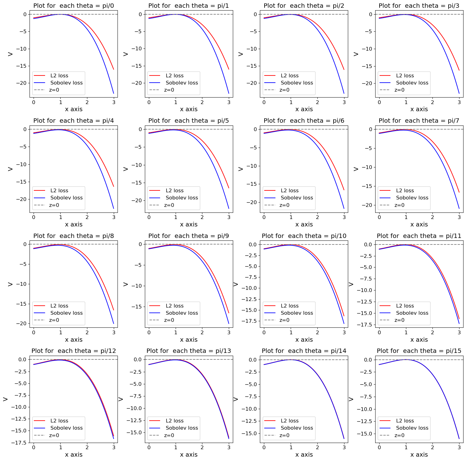
Figure 3: Visualization of comparison between loss function landscape for fixed $\theta\in[0,\pi]$.

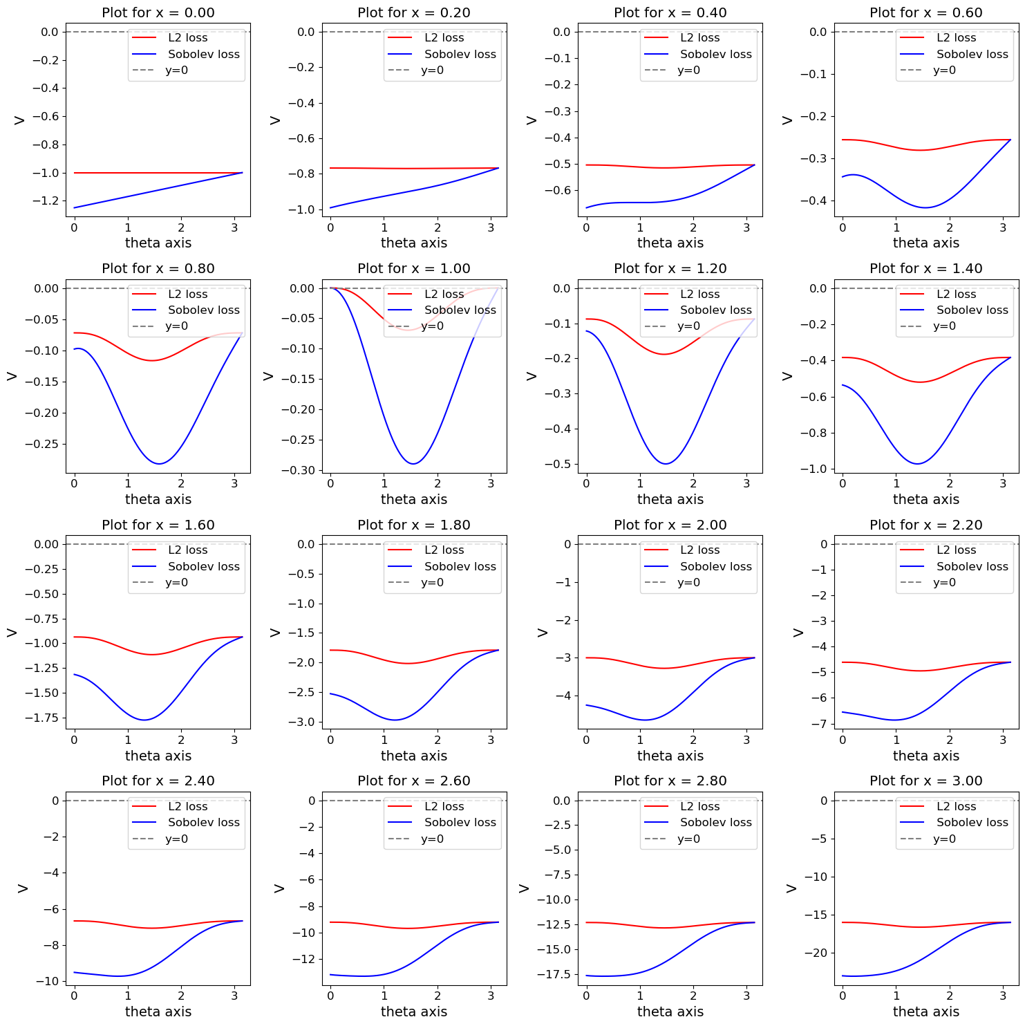
Figure 4: Visualization of comparison between loss function landscape for fixed $x\in[0,3]$.

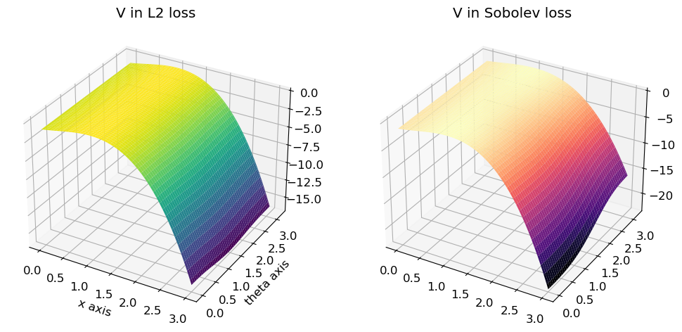
Figure 5: Visualization of loss function landscape for $L^{2}$ loss and Sobolev loss in 3D.

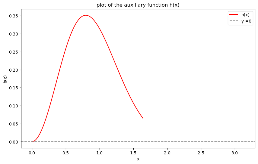
Figure 6: Visualization of $h(\theta)$ define in Equation 27. Note the $h(\theta)$ is not defined for all $\theta\in[0,\pi]$ because we need to exclude the case when $M_{2}^{2}+3M_{1}M_{3}<0$.

References

- Arora et al. (2018) Arora, S., Cohen, N., Golowich, N., and Hu, W. A convergence analysis of gradient descent for deep linear neural networks. arXiv preprint arXiv:1810.02281, 2018.
- Bartlett et al. (2018) Bartlett, P., Helmbold, D., and Long, P. Gradient descent with identity initialization efficiently learns positive definite linear transformations by deep residual networks. In International conference on machine learning, pp. 521–530. PMLR, 2018.
- Cao (2021) Cao, S. Choose a transformer: Fourier or galerkin. Advances in neural information processing systems, 34:24924–24940, 2021.
- Czarnecki et al. (2017) Czarnecki, W. M., Osindero, S., Jaderberg, M., Swirszcz, G., and Pascanu, R. Sobolev training for neural networks. Advances in neural information processing systems, 30, 2017.
- Dosovitskiy et al. (2020) Dosovitskiy, A., Beyer, L., Kolesnikov, A., Weissenborn, D., Zhai, X., Unterthiner, T., Dehghani, M., Minderer, M., Heigold, G., Gelly, S., et al. An image is worth 16x16 words: Transformers for image recognition at scale. arXiv preprint arXiv:2010.11929, 2020.
- Evans (2022) Evans, L. C. Partial differential equations, volume 19. American Mathematical Society, 2022.
- Hao et al. (2022) Hao, Z., Liu, S., Zhang, Y., Ying, C., Feng, Y., Su, H., and Zhu, J. Physics-informed machine learning: A survey on problems, methods and applications. arXiv preprint arXiv:2211.08064, 2022.
- Hao et al. (2023) Hao, Z., Wang, Z., Su, H., Ying, C., Dong, Y., Liu, S., Cheng, Z., Song, J., and Zhu, J. Gnot: A general neural operator transformer for operator learning. In International Conference on Machine Learning, pp. 12556–12569. PMLR, 2023.
- Jagtap & Karniadakis (2020) Jagtap, A. D. and Karniadakis, G. E. Extended physics-informed neural networks (xpinns): A generalized space-time domain decomposition based deep learning framework for nonlinear partial differential equations. Communications in Computational Physics, 28(5), 2020.
- Kenton & Toutanova (2019) Kenton, J. D. M.-W. C. and Toutanova, L. K. Bert: Pre-training of deep bidirectional transformers for language understanding. In Proceedings of NAACL-HLT, pp. 4171–4186, 2019.
- Kovachki et al. (2021) Kovachki, N., Li, Z., Liu, B., Azizzadenesheli, K., Bhattacharya, K., Stuart, A., and Anandkumar, A. Neural operator: Learning maps between function spaces. arXiv preprint arXiv:2108.08481, 2021.
- Lewis et al. (2019) Lewis, M., Liu, Y., Goyal, N., Ghazvininejad, M., Mohamed, A., Levy, O., Stoyanov, V., and Zettlemoyer, L. Bart: Denoising sequence-to-sequence pre-training for natural language generation, translation, and comprehension. arXiv preprint arXiv:1910.13461, 2019.
- Li & Yuan (2017) Li, Y. and Yuan, Y. Convergence analysis of two-layer neural networks with relu activation. Advances in neural information processing systems, 30, 2017.
- Li et al. (2021) Li, Z., Kovachki, N. B., and Azizzadenesheli, K. Burigede liu, kaushik bhattacharya, andrew stuart, and anima anandkumar. Fourier neural operator for parametric partial differential equations. In International Conference on Learning Representations, 2021.
- Li et al. (2022) Li, Z., Huang, D. Z., Liu, B., and Anandkumar, A. Fourier neural operator with learned deformations for pdes on general geometries. arXiv preprint arXiv:2207.05209, 2022.
- Liang & Zhao (2013) Liang, J. and Zhao, H. Solving partial differential equations on point clouds. SIAM Journal on Scientific Computing, 35(3):A1461–A1486, 2013.
- Lipman et al. (2006) Lipman, Y., Cohen-Or, D., and Levin, D. Error bounds and optimal neighborhoods for mls approximation. In Proceedings of the fourth Eurographics symposium on Geometry processing, pp. 71–80, 2006.
- Liu et al. (2020) Liu, Y., Gao, Y., and Yin, W. An improved analysis of stochastic gradient descent with momentum. Advances in Neural Information Processing Systems, 33:18261–18271, 2020.
- Lu et al. (2021) Lu, L., Jin, P., Pang, G., Zhang, Z., and Karniadakis, G. E. Learning nonlinear operators via deeponet based on the universal approximation theorem of operators. Nature machine intelligence, 3(3):218–229, 2021.
- Lu et al. (2017) Lu, Z., Pu, H., Wang, F., Hu, Z., and Wang, L. The expressive power of neural networks: A view from the width. Advances in neural information processing systems, 30, 2017.
- Newman & Barkema (1999) Newman, M. E. and Barkema, G. T. Monte Carlo methods in statistical physics. Clarendon Press, 1999.
- Niemeyer & Geiger (2021) Niemeyer, M. and Geiger, A. Giraffe: Representing scenes as compositional generative neural feature fields. In Proceedings of the IEEE/CVF Conference on Computer Vision and Pattern Recognition, pp. 11453–11464, 2021.
- Ord & Stuart (1994) Ord, K. and Stuart, A. Kendall’s advanced theory of statistics: Distribution theory, 1994.
- Press (2007) Press, W. H. Numerical recipes 3rd edition: The art of scientific computing. Cambridge university press, 2007.
- Radford et al. (2018) Radford, A., Narasimhan, K., Salimans, T., Sutskever, I., et al. Improving language understanding by generative pre-training. 2018.
- Raissi et al. (2019) Raissi, M., Perdikaris, P., and Karniadakis, G. Physics-informed neural networks: A deep learning framework for solving forward and inverse problems involving nonlinear partial differential equations. Journal of Computational Physics, 378:686–707, 2019. ISSN 0021-9991. doi: https://doi.org/10.1016/j.jcp.2018.10.045. URL https://www.sciencedirect.com/science/article/pii/S0021999118307125.
- Son et al. (2023) Son, H., Jang, J. W., Han, W. J., and Hwang, H. J. Sobolev training for physics informed neural networks. Communications in Mathematical Sciences, 21:1679–1705, 2023.
- Tian (2017) Tian, Y. An analytical formula of population gradient for two-layered relu network and its applications in convergence and critical point analysis. In International conference on machine learning, pp. 3404–3413. PMLR, 2017.
- Vaswani et al. (2017) Vaswani, A., Shazeer, N., Parmar, N., Uszkoreit, J., Jones, L., Gomez, A. N., Kaiser, Ł., and Polosukhin, I. Attention is all you need. Advances in neural information processing systems, 30, 2017.
- Yu et al. (2020) Yu, T., Kumar, S., Gupta, A., Levine, S., Hausman, K., and Finn, C. Gradient surgery for multi-task learning. Advances in Neural Information Processing Systems, 33:5824–5836, 2020.
- Zappala et al. (2021) Zappala, E., Levine, D., He, S., Rizvi, S., Levy, S., and van Dijk, D. Operator learning meets numerical analysis: Improving neural networks through iterative methods. arXiv preprint arXiv:2310.01618, 2021.