The Order Oracle: a New Concept in The Black Box Optimization Problems

Abstract

Frequently, the burgeoning field of black-box optimization encounters challenges due to a limited understanding of the mechanisms of the objective function. In this paper, we provide the new concept of the “Order Oracle” as a novel approach to solving such problems. The Order Oracle offers a unique perspective, using only access to the order between function values (possibly with some bounded noise), but without assuming access to their values. As theoretical results, we provide estimates of the convergence rates of the algorithms (obtained by integrating the Order Oracle into existing optimization “tools”) in the non-convex, convex, and strongly convex settings. Our theoretical results demonstrate the effectiveness of the Order Oracle through numerical experiments. Finally, we show the possibility of accelerating the convergence of such algorithms.

1 Introduction

The black box problem has garnered extensive attention in diverse scientific and engineering domains, reflecting the challenge of optimizing systems with complex and opaque objective functions, prompting the exploration of innovative solutions Conn et al. (2009); Kimiaei & Neumaier (2022).

This paper focuses on solving a standard general optimization problem in the following form:

$$\min_{x\in\mathbb{R}^{d}}\left\{f(x):=\mathbb{E}_{\xi\sim\mathcal{D}}f_{\xi}(x)\right\},$$ (1)

where $f:\mathbb{R}^{d}\rightarrow\mathbb{R}$ is a possibly non-convex, possibly stochastic function. This configuration of problem encompasses a broad range of applications in machine learning scenarios, such as the empirical risk minimization (ERM), where $\mathcal{D}$ denotes the distribution across training data points, and $f_{\xi}(x)$ represents the loss of model $x$ on data point $\xi$.

When the objective function $f(x)$ has exclusive access to a zero-order oracle Rosenbrock (1960), problem (1) falls under the classification of a black-box optimization problem. This class of problems is actively studied in various application settings, e.g., deep learning Chen et al. (2017); Gao et al. (2018), federated learning Dai et al. (2020); Alashqar et al. (2023); Patel et al. (2022), reinforcement learning Choromanski et al. (2018); Mania et al. (2018), overparameterized models Lobanov & Gasnikov (2023), online optimization (Agarwal et al., 2010; Bach & Perchet, 2016; Akhavan et al., 2022), multi-armed bandits Shamir (2017); Lattimore & Gyorgy (2021), hyperparameter settings Bergstra & Bengio (2012); Hernández-Lobato et al. (2014); Nguyen & Balasubramanian (2022), and control system performance optimization Bansal et al. (2017); Xu et al. (2022). It is important to highlight that the zero-order oracle presupposes awareness of the objective function’s value $f(x_{k})$ at a specific point $x_{k}$ (which may be inexact), enabling the development of effective gradient-free algorithms tailored to various problem scenarios Gasnikov et al. (2022a).

Table 1: Comparison of the methods proposed in this work with SOTA first-order methods in the coordinate descent class. Notation: $F_{0}=f(x_{0})-f(x^{*})$; $R_{[1-\alpha]}=R_{1-\alpha}(x_{0})=\sup_{x\in\mathbb{R}^{d}:f(x)\leq f(x_{0})}\left\|x-x^{*}\right\|_{[1-\alpha]}$; $\varepsilon=$ desired accuracy of problem solving.

Function	Non-convex	Convex		Strongly convex
Reference	Theorem 3.1	Nesterov (2012)	Theorem 3.2	Nesterov (2012)	Theorem 3.3		Nesterov & Stich (2017)	Theorem 4.1
# iterations	$\mathcal{O}\left(\frac{S_{\alpha}F_{0}}{\varepsilon^{2}}\right)$	$\mathcal{O}\left(\frac{S_{\alpha}R^{2}_{[1-\alpha]}}{\varepsilon}\right)$	$\mathcal{O}\left(\frac{S_{\alpha}R^{2}_{[1-\alpha]}}{\varepsilon}\right)$	$\mathcal{O}\left(\frac{S_{\alpha}}{\mu_{1-\alpha}}\log\frac{1}{\varepsilon}\right)$	$\mathcal{O}\left(\frac{S_{\alpha}}{\mu_{1-\alpha}}\log\frac{1}{\varepsilon}\right)$		$\mathcal{O}\left(\frac{S_{\alpha/2}}{\sqrt{\mu_{1-\alpha}}}\log\frac{1}{\varepsilon}\right)$	$\mathcal{O}\left(\frac{S_{\alpha/2}}{\sqrt{\mu_{1-\alpha}}}\log\frac{1}{\varepsilon}\right)$
# oracles	$\tilde{\mathcal{O}}\left(\frac{S_{\alpha}F_{0}}{\varepsilon^{2}}\right)$	$\mathcal{O}\left(\frac{S_{\alpha}R^{2}_{[1-\alpha]}}{\varepsilon}\right)$	$\tilde{\mathcal{O}}\left(\frac{S_{\alpha}R^{2}_{[1-\alpha]}}{\varepsilon}\right)$	$\mathcal{O}\left(\frac{S_{\alpha}}{\mu_{1-\alpha}}\log\frac{1}{\varepsilon}\right)$	$\tilde{\mathcal{O}}\left(\frac{S_{\alpha}}{\mu_{1-\alpha}}\log\frac{1}{\varepsilon}\right)$		$\mathcal{O}\left(\frac{S_{\alpha/2}}{\sqrt{\mu_{1-\alpha}}}\log\frac{1}{\varepsilon}\right)$	$\tilde{\mathcal{O}}\left(\frac{S_{\alpha/2}}{\sqrt{\mu_{1-\alpha}}}\log\frac{1}{\varepsilon}\right)$
Order Oracle?	✓	✗	✓	✗	✓		✗	✓
Acceleration?	✗	✗	✗	✗	✗		✓	✓

In this paper, we introduce a new concept of a zero-order oracle, termed the Order Oracle, to address problem (1):

$$\phi(x,y)=\text{sign}\left[f(x)-f(y)+\delta(x,y)\right],$$ (2)

where $|\delta(x,y)|\leq\Delta$ is some bounded noise. The Order Oracle has the capability to compare two functions; however, in contrast to the zero-order oracle, it lacks the ability to calculate or utilize the actual value of the objective function. This concept closely mirrors the challenges encountered in real-world black-box optimization problems.

Figure 1: Valio’s chocolate

The motivation for the proposed oracle concept becomes more evident when considering the ongoing developments in generative models. Companies like Valio and SberAI have already embraced the active involvement of AI in dessert creation. Notably, Valio, as illustrated in Figure 1, employed AI to determine the optimal concentration of milk for chocolate bars based on available data. However, envision a scenario where AI creates customized chocolate for an individual by adjusting the concentration of ingredients. In such a case, a flavor comparison procedure, depicted in one iteration, would involve determining the preference order. Given that tastes can be closely aligned, introducing bounded noise in oracle (2) mitigates the potential for errors.

To address the initial problem (1) with the Order Oracle (2), we center our focus on the coordinate descent methods (CD) class Bubeck et al. (2015), utilizing it as a pivotal optimization “tool” to integrate our oracle into multidimensional optimization, thereby presenting a novel and efficient algorithm. Our approach involves employing a linear search, which operates based on the order of objective functions (comparing two functions), to ascertain a parameter $\eta_{k}$. This parameter encapsulates both the step size and the gradient coordinate of the objective function. Consequently, we offer not merely an optimization method exclusively leveraging the Order Oracle but also an adaptive approach that determines both the step size and the values of the directional derivative using one of the linear search algorithms.

1.1 Our contributions

More specifically, our contributions are the following:

• We introduce the Order Oracle (2), a novel concept of zero-order oracle that closely mirrors real-world scenarios, opening promising avenues in black-box optimization. Additionally, we devise an approach to develop efficient algorithms to solve problems (1) solely based on function order, rather than their explicit values.

• We present a new algorithm in the class of coordinate descent methods, leveraging the oracle proposed in this paper: Random Coordinate Descent with Order Oracle (OrderRCD), Algorithm 1. This algorithm can be classified as adaptive since it does not depend on information about the step size or the gradient coordinate value. We analyze the convergence of this algorithm across non-convex, convex, and strongly convex settings, assuming function smoothness. Our results demonstrate the effectiveness of this algorithm, with competitive convergence scores observed among SOTA first-order algorithms (see Table 1, columns without acceleration).

• We have demonstrated that even with an oracle like the Order Oracle (2), acceleration is achievable. This is evidenced by the convergence results of the Accelerated Coordinate Descent Method with Order Oracle (OrderACDM) Algorithm 2 (see Table 1, last column).

• Through numerical experiments, we validate our theoretical results, demonstrating that the proposed algorithms are not only comparable to, but sometimes superior to their competitors in terms of iteration complexity, thanks to adaptive step selection. Additionally, we explicitly showcase the potential for speedup in the Order Oracle concept and provide practical recommendations for its implementation.

1.2 Main assumptions and notations

Before discussing related works, we present the notation and main assumptions we use in our work.

Notation.

We use $\left\langle x,y\right\rangle:=\sum_{i=1}^{d}x_{i}y_{i}$ to denote standard inner product of $x,y\in\mathbb{R}^{d}$. We denote Euclidean norm in $\mathbb{R}^{d}$ as $\|x\|:=\sqrt{\sum_{i=1}^{d}x_{i}^{2}}$. In particular, this norm ${\|x\|:=\sqrt{\left\langle x,x\right\rangle}}$ is related to the inner product as . We use $\mathbf{e}_{i}\in\mathbb{R}^{d}$ to denote the $i$-th unit vector. We define the norms ${\|\cdot\|_{[\alpha]}:=\sqrt{\sum_{i=1}^{d}L_{i}^{\alpha}x_{i}^{2}}}$ and ${\|\cdot\|_{[\alpha]}^{*}:=\sqrt{\sum_{i=1}^{d}\frac{1}{L_{i}^{\alpha}}x_{i}^{2}}}$. We denote by $\nabla f(x)$ the full gradient of objective function $f$ at point $x\in\mathbb{R}^{d}$, and by $\nabla_{i}f(x)$ the $i$-th coordinate gradient. The sum of constant smoothness $L_{i}$ denotes as $\overline{L}:=\sum_{i}^{d}L_{i}$ and $S_{\alpha}:=\sum_{i}^{d}L_{i}^{\alpha}$. We use the notation $\tilde{O}(\cdot)$ to hide the logarithmic coefficients. We denote $f^{*}:=f(x^{*})$ as the solution to initial problem.

For all our theoretical results, we assume that $f(x)$ is $L_{i}$-smooth with respect to its $i$-th coordinate:

Assumption 1.1 (Smoothness).

A function $f:\mathbb{R}^{d}\rightarrow\mathbb{R}$ is $L$-coordinate-Lipschitz for $L_{1},L_{2},...,L_{d}>0$ if for any $i\in[d],x\in\mathbb{R}^{d}$ and $h\in\mathbb{R}$ the following inequality holds:

$$|\nabla_{i}f(x+h\mathbf{e}_{i})-\nabla_{i}f(x)|\leq L_{i}|h|.$$

The smoothness assumption of the function is widely used in the optimization literature (e.g. Boyd & Vandenberghe, 2004; Nesterov et al., 2018). However, Assumption 1.1 is specific and frequently utilized in the context of optimization via the coordinate descent method Lin et al. (2014); Zhang & Xiao (2017); Mangold et al. (2023). This assumption means that for every input point $x$, if we alter its $i$-th coordinate by at most $h$, then the corresponding gradient $\nabla_{i}f(x+h\mathbf{e}_{i})$ differs from $\nabla_{i}f(x)$ by at most $L_{i}$ times $|h|$.

Throughout this paper we assume that the objective function $f(x)$ can be (strongly) convex w.r.t. the norm $\left\|\cdot\right\|_{[1-\alpha]}$:

Assumption 1.2.

A function $f:\mathbb{R}^{d}\rightarrow\mathbb{R}$ is $\mu_{1-\alpha}\geq 0$ strongly convex w.r.t. the norm $\left\|\cdot\right\|_{[1-\alpha]}$ if for any ${x,y\in\mathbb{R}^{d}}$ the following inequality holds:

$$f(y)\geq f(x)+\left\langle\nabla f(x),y-x\right\rangle+\frac{\mu_{1-\alpha}}{2}\left\|y-x\right\|_{[1-\alpha]}^{2}.$$

Many works in convex optimization rely on the (strong) convexity assumption, as evidenced by references such as Duchi (2016); Shi et al. (2019); Asi et al. (2021). Since our work employs norms $\left\|\cdot\right\|_{[1-\alpha]}$ to derive theoretical estimates, Assumption 1.2 deviates slightly from the standard. However, this assumption of $\mu_{1-\alpha}$ (strong) convexity is extensively used in the following literature: Nesterov (2012); Lee & Sidford (2013); Allen-Zhu et al. (2016); Mangold et al. (2022). Assumption 1.2 can conform to the standard form of $\mu$ (strong) convexity via the Euclidean norm if $\alpha=1$. In addition, this assumption is convex provided $\mu_{1-\alpha}=0$.

1.3 Paper organization

Further, this paper has the following structure. In Section 2, we provide a related work discussion. We present and analyze the non-accelerated algorithm in Section 3. Then in Section 4, we discuss the feasibility of accelerating the proposed algorithm in the concept of Order Oracle and provide theoretical guarantees. In Section 5, we discuss the current results of this work. Through numerical experiments in Section 6, we validate the theoretical results. While Section 7 concludes the paper. The detailed proofs of all theorems are presented in the Supplementary Materials (Appendix).

2 Related Works

The literature in the field of optimization is already extensive and continuously expanding, encompassing various problem formulations and assumptions. In this section, we provide an overview of the most relevant contributions to our work.

Oracle concepts.

One of the key criteria for evaluating optimization algorithms is oracle complexity. Oracles are commonly used in theoretical estimates, where they offer insights into the function’s behavior. For instance, the first-order oracle is prevalent in machine learning literature: the authors of Gorbunov et al. (2020); Gurbuzbalaban et al. (2021); Huang et al. (2022) use the oracle to obtain the gradient value $\nabla f(x_{k})$ of a function at a given point $x_{k}$. And in Stich & Karimireddy (2020); Ajalloeian & Stich (2020); Glasgow et al. (2022), the authors assume some adversarial environment where the oracle is inaccurate, i.e., the oracle produces the gradient of the function at a given point with some adversarial noise (adversarial refers to the noise that accumulates over iterations). The authors of Nesterov (2012); Lee & Sidford (2013); Mangold et al. (2023) also refer their oracles that produce only the gradient coordinate of the function $\nabla_{i}f(x_{k})$ at a given point $x_{k}$ to a first-order oracle. However, this oracle formally can also be referred to the so-called gradient-free oracle Gasnikov et al. (2022a), since the algorithm does not use the whole gradient, but only the directional derivative. The following works Jiang et al. (2019); Nesterov (2021); Agafonov et al. (2023) use a higher-order oracle to obtain information, for example, about the Hesse matrix of a function at a given point. But there are oracle concepts closer to reality, for example in Bach & Perchet (2016); Shamir (2017); Akhavan et al. (2021); Gasnikov et al. (2022b); Kornilov et al. (2023) the authors develop algorithms that use only information about the function value $f(x)$, possibly with some adversarial noise. Such a concept is very common in the field of black-box optimization. In this paper we propose a new concept of zero-order oracle: the Order Oracle (2), which is even closer to reality, where even the function value is not available to us, but only the order between two functions (the possibility to compare). Moreover, we take into account the presence of noise (which seems to be natural in applied realities) in such an oracle.

Coordinate methods.

In addition to full-gradient algorithms for smooth first-order optimization, coordinate descent algorithms are categorized into accelerated and non-accelerated algorithms. Non-accelerated algorithms typically converge at rates $1/\varepsilon$ and $1/\mu$ in convex ($\mu=0$) and strongly convex ($\mu>0$) cases, respectively, while accelerated algorithms achieve rates $1/\sqrt{\varepsilon}$ and $1/\sqrt{\mu}$ in convex and strongly convex cases, respectively. This classification dates back to 1983 when Nesterov introduced the optimal convergence rates for first-order algorithms Nesterov (1983). However, the fundamental difference between coordinate descent and full-gradient descent lies in the step taken along the $i$-th coordinate of the gradient (directional derivative). Monograph Bubeck et al. (2015) has demonstrated that if the direction is chosen uniformly, coordinate descent may require up to $d$ times more iterations than full-gradient descent. However, authors in Nesterov (2012) have shown that considering smoothness along the direction $L_{i}$ can improve the number of iterations $\mathcal{O}\left(\frac{S_{\alpha}R^{2}_{[1-\alpha]}}{\varepsilon}\right)$ and $\mathcal{O}\left(\frac{S_{\alpha}}{\mu_{1-\alpha}}\log\frac{1}{\varepsilon}\right)$ in convex and strongly convex cases, respectively, where $R_{[1-\alpha]}=\sup_{x\in\mathbb{R}^{d}:f(x)\leq f(x_{0})}\left\|x-x^{*}\right\|_{[1-\alpha]}$ for $\alpha\in[0,1]$. In the same paper Nesterov (2012), the authors demonstrated the potential for acceleration in coordinate descent through the scheme proposed in Nesterov (1983). Subsequently, in Lee & Sidford (2013), they analyzed and presented an accelerated version of coordinate descent (ACDM), along with the corresponding number of required $\tilde{\mathcal{O}}\left(\sqrt{\frac{dS_{\alpha}R^{2}_{[1-\alpha]}}{\varepsilon}}\right)$ and $\mathcal{O}\left(\sqrt{\frac{dS_{\alpha}}{\mu_{1-\alpha}}}\log\frac{1}{\varepsilon}\right)$ iterations in convex and strongly convex cases, respectively. It is noteworthy that, at that time, this iteration complexity was deemed unimprovable. However, a few years later, both Nesterov & Stich (2017) and Allen-Zhu et al. (2016) independently provided same results, demonstrating that it is indeed possible to enhance the iteration complexity for accelerated coordinate descent methods by modifying the probability of choosing the $i$-th coordinate: $L_{i}^{\alpha/2}/S_{\alpha/2}$. In this paper, we propose a coordinate descent algorithm with an Order Oracle (2), demonstrating that it achieves the same iteration complexity as first-order algorithms. Furthermore, based on accelerated coordinate descent Nesterov & Stich (2017), we establish on the strongly convex case that even with an Order Oracle, acceleration can be attained, resulting in the most favorable estimates on iteration complexity known to date.

Adaptability.

The trend towards developing adaptive algorithms is steadily gaining momentum, with numerous works dedicated to this emerging field. Among the various facets of adaptability explored in the literature, three tracks stand out: adaptability to algorithm step selection Duchi et al. (2011); Li & Orabona (2020); Faw et al. (2022); Kavis et al. (2022); Liu et al. (2023); Huang et al. (2023), adaptability to oracle inaccuracy Agarwal et al. (2011); Belloni et al. (2015); Risteski & Li (2016); Bubeck et al. (2017); Ajalloeian & Stich (2020); Gasnikov et al. (2022b); Kornilov et al. (2023), and adaptability to noise with heavy tails Nazin et al. (2019); Gorbunov et al. (2020); Cutkosky & Mehta (2021); Hodgkinson & Mahoney (2021); Li & Liu (2022); Sadiev et al. (2023); Puchkin et al. (2023). It’s noteworthy that the latter two tracks can be viewed as adaptability to adversarial attacks Fawzi et al. (2016); Li et al. (2019), adding further motivation to research efforts. This categorization of adaptability is corroborated by the increasing amount of research within the community. In our work, we focus on the adaptability of choosing the step size and gradient coordinate value in coordinate descent, by using linear search, since this class of methods fits the concept of the Order Oracle, and the step size together with the gradient coordinate value are scalars. We chose the Golden Ratio algorithm as the linear search method because this algorithm performs well in solving auxiliary optimization problems Alacaoglu et al. (2023). We also study the issue of adaptability to oracle inaccuracy, i.e., we provide conditions on the noise level (to which the Order Oracle is subject) under which “good” convergence is guaranteed. By “good” we mean convergence with $\Delta=0$.

3 Non-Accelerated Methods

In this section, we begin to present the main results of the paper, by introducing optimization algorithms tailored to address the initial problem (1) utilizing the Order Oracle (2). Given the novelty of this oracle concept, we furnish convergence guarantees and conduct comparisons with algorithms employing alternative oracles.

Our approach for developing a new algorithm involves incorporating the Order Oracle into an existing optimization method using linear search. We opt for linear search as the integration tool due to its compatibility with the Order Oracle concept. However, the choice of optimization method to which this linear search can be applied poses a crucial question. After careful consideration, we determined that the coordinate descent method (CDM) is the most suitable candidate. In each iteration, the CDM, given a step size $\zeta_{k}>0$ and starting point $x_{0}\in\mathbb{R}^{d}$, proceeds as follows:

$$x_{k+1}=x_{k}-\underbrace{\zeta_{k}\nabla_{i_{k}}f(x_{k})}_{\eta_{k}}\mathbf{e}_{i_{k}},$$ (3)

where $i_{k}$ is the coordinate index drawn from $[d]$. Note that the coordinate descent method step (3) requires both a step size $\zeta_{k}$ and a gradient coordinate value $\nabla_{i_{k}}f(x_{k})$, which are scalars. Thus, by employing linear search ${\eta_{k}=\operatorname*{arg\,min}_{\eta}\{f(x_{k}+\eta\mathbf{e}_{i_{k}})\}}$ at each iteration, we can optimally determine both the direction of steepest descent and the step size to traverse along this direction, resulting in a fully adaptive algorithm. The next consideration is the strategy for coordinate selection at each iteration. Following the trend initiated by Nesterov (2012), we use a more general sampling distribution than the uniform one, obtaining already random coordinate descent (RCD). Specifically, for $\alpha>0$, we assume that a random generator $\mathcal{R}_{\alpha}(L)$ independently selects $i_{k}$ from the following distribution:

$$p_{\alpha}(i)=L_{i}^{\alpha}/S_{\alpha},\quad i\in[d].$$ (4)

We are now ready to introduce a optimization method designed to solve problem (1) utilizing the oracle concept (2).

  Input: $x_{0}\in\mathbb{R}^{d}$, random generator $\mathcal{R}_{\alpha}(L)$

  for $k=0$ to $N-1$ do

     1.   choose active coordinate $i_{k}=\mathcal{R}_{\alpha}(L)$

     2.   compute $\eta_{k}=\text{argmin}_{\eta}\{f(x_{k}+\eta\mathbf{e}_{i_{k}})\}$ via (GRM)

     3.   $x_{k+1}\leftarrow x_{k}+\eta_{k}\mathbf{e}_{i_{k}}$

  end for

  Return: $x_{N}$

Algorithm 1 Random Coordinate Descent with Order Oracle (OrderRCD)

This algorithm falls under the category of coordinate methods and is named random coordinate descent with order oracle (OrderRCD), see Algorithm 1. The golden ratio method (GRM) serves as the linear search algorithm. It should be noted that the inherent “stochasticity” of the problem (1) is artificially induced by the randomized procedure used to select the $i$-th coordinate (4). Here, $\xi$ denotes the $i$-th coordinate, and $\mathcal{D}$ represents the distribution $p_{\alpha}(i)$ from (4).

Next, we present our theoretical results, demonstrating through convergence analyses that random coordinate descent with order oracle (OrderRCD) exhibits competitive iteration complexity compared to first-order algorithms when applied to non-convex, convex, or strongly convex functions.

3.1 Non-convex setting

Theorem 3.1 (non-convex).

Let function f(x) satisfies Assumption 1.1, then Algorithm 1 (OrderRCD) with oracle (2) guarantees an error in the case $\Delta=0$:

$$\frac{1}{N}\sum_{k=0}^{N-1}\left(\left\|\nabla f(x_{k})\right\|_{[1-\alpha]}^{*}\right)^{2}\leq\mathcal{O}\left(\frac{S_{\alpha}F_{0}}{N}\right),$$

where $N$ is the number of iterations, $F_{0}=f(x_{0})-f(x^{*})$.

The convergence results of Theorem 3.1 imply the existence of a point $k\in[N]$ where $(\left\|\nabla f(x_{k})\right\|_{[1-\alpha]}^{*})^{2}\leq\mathcal{O}\left(\frac{S_{\alpha}F_{0}}{N}\right)$ holds true. Additionally, Theorem 3.1 indicate that, to achieve the desired accuracy $\varepsilon$ (according to the gradient norm), Algorithm 1 requires $N=\mathcal{O}\left(S_{\alpha}F_{0}/\varepsilon^{2}\right)$ iterations and $T=\tilde{\mathcal{O}}\left(S_{\alpha}F_{0}/\varepsilon^{2}\right)$ calls to the oracle (2). The maximum admissible noise level ensuring the desired accuracy should not exceed $\sim\varepsilon^{2}$. Notably, the convergence rate of random coordinate descent with the order oracle (OrderRCD), assuming minimal noise ($\Delta\leq\varepsilon^{2}$), is equal to first-order method: random coordinate descent (RCD). It is also characteristic (within the coordinate methods class) to be inferior to gradient descent (Ghadimi & Lan, 2013, under $L$ smoothness assumption). For instance, in the case when $\alpha=1$, the convergence rates $\mathcal{O}\left(LF_{0}/N\right)$ is better because $L\leq\sum_{i=1}^{d}L_{i}=\overline{L}$. Not surprisingly, in terms of oracle complexity, Algorithm (1) is logarithmically inferior to first-order algorithms in the non-convex case. This discrepancy reflects the “cost” associated with employing the Order Oracle concept (2), where the $\tilde{O}(\cdot)$ to hide the logarithmic coefficient representing the number of oracle calls in the golden ratio method (GRM), contingent upon its accuracy. A detailed proof of Theorem 3.1 is given in Appendix B.1.

3.2 Convex setting

We now prove an analogous theorem on the convergence of the algorithm when the function is convex, i.e., additionally assuming that Assumption 1.2 is satisfied with $\mu_{1-\alpha}=0$.

Theorem 3.2 (convex).

Let function $f(x)$ satisfies Assumption 1.1 ($L$-coordinate-Lipschitz) and Assumption 1.2 (convexity, $\mu_{1-\alpha}=0$), then Algorithm 1 (OrderRCD) with oracle (2) guarantees an error in the case $\Delta=0$:

$$\mathbb{E}\left[f(x_{N})\right]-f(x^{*})\leq\mathcal{O}\left(\frac{S_{\alpha}R^{2}_{[1-\alpha]}}{N}\right),$$

where $\alpha>0$, ${R_{[1-\alpha]}=\sup_{x\in\mathbb{R}^{d}:f(x)\leq f(x_{0})}\left\|x-x^{*}\right\|_{[1-\alpha]}}$, ${S_{\alpha}=\sum_{i=1}^{d}=L_{i}^{\alpha}}$, and ${x^{*}=\operatorname*{arg\,min}_{x}f(x)}$.

In comparison to Theorem 3.1 (non-convex setting), the convergence results of Algorithm 1 demonstrate improvement under the assumption of function convexity (Assumption 1.2 with $\mu_{1-\alpha}=0$). Specifically, according to Theorem 3.2, random coordinate descent with order oracle (OrderRCD) requires $N=\mathcal{O}(S_{\alpha}R^{2}_{[1-\alpha]}/\varepsilon)$ iterations and $T=\tilde{\mathcal{O}}(S_{\alpha}R^{2}_{[1-\alpha]}/\varepsilon)$ oracle calls to achieve the desired accuracy $\varepsilon$ (where $\mathbb{E}\left[f(x_{N})\right]-f(x^{*})\leq\varepsilon$). However, in cases where $\Delta>0$, the condition for maximum noise remains unchanged compared to the non-convex setting. Furthermore, the iteration complexity $N$ aligns with that of the first-order algorithm, (random coordinate descent (RCD) Nesterov, 2012). Similarly, akin to Theorem 3.2, the convergence rate of gradient descent (Nesterov et al., 2018, under assuming $L$ smoothness and convexity) outperforms that of Algorithm 1. Moreover, when $\alpha=0$ (corresponding to a uniform distribution with probability $p_{\alpha}(i)=1/d$), OrderRCD (like all coordinate methods) necessitates $d$ times more iterations than gradient descent. Concerning oracle complexity $T$, a logarithmic coefficient is evident, correlating with the number of oracle calls per iteration of Algorithm 1. For a comprehensive proof of Theorem, refer to Appendix B.2.

3.3 Strongly convex setting

In this section we consider the case when the function is strongly convex (see Assumption 1.2 with $\mu_{1-\alpha}>0$).

Theorem 3.3 (strongly convex).

Let function $f(x)$ satisfies Assumption 1.1 ($L$-coordinate-Lipschitz) and Assumption 1.2 (convexity, $\mu_{1-\alpha}>0$), then Algorithm 1 with oracle (2) (in the case $\Delta=0$) has a linear convergence rate:

$$\mathbb{E}\left[f(x_{N})\right]-f(x^{*})\leq\left(1-\frac{\mu_{1-\alpha}}{S_{\alpha}}\right)^{N}F_{0}.$$

As depicted in Theorem 3.3, in the strongly convex setting, Algorithm 1 exhibits a linear convergence rate, achieving the desired accuracy $\varepsilon$ in $N=\mathcal{O}\left(S_{\alpha}/\mu_{1-\alpha}\log\frac{1}{\varepsilon}\right)$ iterations and $T=\tilde{\mathcal{O}}\left(S_{\alpha}/\mu_{1-\alpha}\log\frac{1}{\varepsilon}\right)$ oracle calls. Furthermore, there’s an enhancement in the maximum noise level $\Delta$, reaching ${\sim\mu_{1-\alpha}}\varepsilon$. It’s notable that a weaker strong convexity condition was employed in the proof of Theorem 3.3:

$$\left\|\nabla f(x)\right\|_{[1-\alpha]}^{2}\geq 2\mu_{1-\alpha}(f(x)-f(x^{*})),\forall x\in\mathbb{R}^{d}.$$ (5)

This condition (in the case $\alpha=1$), also known as the Polyak–Lojasiewicz or Gradient-dominated functions condition Polyak (1963); Lojasiewicz (1963); Karimi et al. (2016); Belkin (2021), encompasses a broad class of functions: convex functions, strongly convex functions, sum of squares (e.g. where considering a system of non-linear equations), invex and non-convex functions, as well as over-parameterized systems. Also it is shown in Yue et al. (2023) that non-accelerated algorithms are optimal for $L$-smooth problems under the Polyak–Lojasiewicz condition (5). For a detailed proof of Theorem 3.3, see Appendix B.3.

High probability deviations bounds.

Given that OrderRCD method (see Algorithm 1) in the strongly convex setting demonstrates a linear convergence rate (as per Theorem 3.3) and employs a randomization in coordinate selection, we can derive exact estimates of the high deviation probabilities using Markov’s inequality Anikin et al. (2015):

$$\mathcal{P}\left(f(x_{N(\varepsilon\sigma)})-f^{*}\geq\varepsilon\right)\leq\sigma\frac{\mathbb{E}\left[f(x_{N(\varepsilon\sigma)}\right]-f^{*}}{\varepsilon\sigma}\leq\sigma.$$

4 Accelerated Method

Random coordinate descent with order oracle (OrderRCD) demonstrates efficiency in the class of coordinate methods. The number of iterations $N$ required to achieve the desired accuracy $\varepsilon$ is fully identical to random coordinate descent, which is the best among the non-accelerated methods in this class. This fact confirms that our approach to developing a novel optimization algorithm using only the oracle is successful. However, Algorithm 1 is still not optimal because it belongs to non-accelerated algorithms. Nevertheless, Section 3 gives hope for the possibility of acceleration among algorithms using the new oracle concept (2).

In this section, we demonstrate on the example of the strongly convex (Assumption 1.2 is satisfied with constant $\mu_{1-\alpha}>0$) problem (1) that acceleration in the class of optimization algorithms using the Order Oracle (2) exists. For simplicity, we consider the case when $\Delta=0$.

Our approach to creating an accelerated algorithm closely mirrors the one proposed in Section 3, which involves adapting an existing optimization method (from the class of coordinate algorithms) to the Order Oracle using linear search. Among the accelerated algorithms in the class of coordinate descent, two stand out: (accelerated coordinate descent method (ACDM), Nesterov & Stich, 2017) and (accelerated coordinate descent method with non-uniform sampling (NU-ACDM), Allen-Zhu et al., 2016). These algorithms boast the same convergence rate and are considered among the best available today. Therefore, we select one of them (specifically, ACDM) as the base algorithm to adapt to the new oracle concept (2). At each iteration, the ACDM, given parameters such as $\alpha_{k}$, $\beta_{k}$, $a_{k+1}$, $A_{k+1}$, $B_{k+1}$, Lipschitz coordinate constant $L_{i}$, strong convexity $\mu_{1-\alpha}$, distribution $p_{\beta}(i)$, and a starting point $x_{0}=z_{0}$, proceeds as follows:

$$y_{k}=(1-\alpha_{k})x_{k}+\alpha_{k}w_{k},$$

$$x_{k+1}=y_{k}-(1/L_{i_{k}})\nabla_{i_{k}}f(y_{k})\mathbf{e}_{i_{k}},$$ (6)

$$z_{k+1}=w_{k}-\frac{a_{k+1}}{L_{i_{k}}^{1-\alpha}B_{k+1}p_{\beta}(i)}\nabla_{i_{k}}f(y_{k})\mathbf{e}_{i_{k}},$$ (7)

where $w_{k}=(1-\beta_{k})z_{k}+\beta_{k}y_{k}$. Looking at the $x_{k+1}$ update (6), it seems that it should not be difficult to determine the step size $1/L_{i_{k}}$ and the value of the gradient coordinate $\nabla_{i_{k}}f(y_{k})$ using a linear search, as demonstrated in Algorithm 1. However, substituting the same $\eta_{k}$ instead of $(1/L_{i_{k}})\nabla_{i_{k}}f(y_{k})$ into the $z_{k+1}$ update (7) isn’t straightforward. The step with linear search is larger than the original step of $(1/L_{i_{k}})\nabla_{i_{k}}f(y_{k})$, potentially leading to a paradoxical situation where the step worsens with linear search. This is because there is no guarantee that the function $f$ is monotonically decreasing along the sequences $\{z_{k}\}_{k=0}^{\infty}$ and $\{x_{k}\}_{k=0}^{\infty}$ Nesterov (1983). Nevertheless, we have successfully addressed this challenge and we are ready to present the first (as far as we are aware) accelerated algorithm utilizing only the Order Oracle: the accelerated coordinate descent method with order oracle (OrderACDM).

  Input: $x_{0}=z_{0}\in\mathbb{R}^{d}$, $\mathcal{R}_{\alpha}(L)$, $A_{0}=0$, $B_{0}=1$, $\beta=\frac{\alpha}{2}$

  for $k=0$ to $N-1$ do

     1.   choose active coordinate $i_{k}=\mathcal{R}_{\beta}(L)$

     2.   find parameter $a_{k+1}$ from $a_{k+1}^{2}S_{\beta}^{2}=A_{k+1}B_{k+1}$,

2.   where $A_{k+1}=A_{k}+a_{k+1}$ and

2.   where $B_{k+1}=B_{k}+\mu_{1-\alpha}a_{k+1}$

     3.   $\alpha_{k}\leftarrow\frac{a_{k+1}}{A_{k+1}}$

     4.   $\beta_{k}\leftarrow\frac{\mu_{1-\alpha}a_{k+1}}{B_{k+1}}$

     5.   $y_{k}\leftarrow\frac{(1-\alpha_{k})x_{k}+\alpha_{k}(1-\beta_{k})z_{k}}{1-\alpha_{k}\beta_{k}}$

     6.   compute $\eta_{k}=\text{argmin}_{\eta}\{f(y_{k}+\eta\mathbf{e}_{i_{k}})\}$ via (GRM)

     7.   $x_{k+1}\leftarrow y_{k}+\eta_{k}\mathbf{e}_{i_{k}}$

     8.   $w_{k}\leftarrow(1-\beta_{k})z_{k}+\beta_{k}y_{k}+\frac{a_{k+1}L_{i_{k}}^{\alpha}}{B_{k+1}p_{\beta}(i)}\eta_{k}\mathbf{e}_{i_{k}}$

     9.   compute $\zeta_{k}=\text{argmin}_{\zeta}\{f(w_{k}+\zeta\mathbf{e}_{i_{k}})\}$ via (GRM)

     10.   $z_{k+1}\leftarrow w_{k}+\zeta_{k}\mathbf{e}_{i_{k}}$

  end for

  Return: $x_{N}$

Algorithm 2 Accelerated Coordinate Descent Method with Order Oracle (OrderACDM)

It is evident from Algorithm 2 that the challenge was addressed by incorporating a secondary linear search, ensuring that the update step in $z_{k+1}$ with linear search is at least as effective as (7). However, unlike Algorithm 1, OrderACDM cannot be deemed fully adaptive as it necessitates knowledge of the strong convexity constant $\mu_{1-\alpha}$ and the Lipschitz-coordinate constant $L_{i}$ (which disappears in the case where $\alpha=0$). Despite this, we are ready to present the main advantage of Algorithm 2: Faster convergence rate of Accelerated Coordinate Descent Method with Order Oracle.

Theorem 4.1.

Let function $f(x)$ is strongly convex (Assumption 1.2), $L$-Coordinate-Lipschitz (Assumption 1.1) and $L_{[1-\alpha]}$-Lipschitz-smooth, then Algorithm 2 (OrderACDM) with oracle (2) guarantees an error

$$\mathbb{E}\left[f(x_{N})\right]-f(x^{*})\leq\left(1-\frac{\sqrt{\mu_{1-\alpha}}}{S_{\alpha/2}}\right)^{N}F_{0},$$

where $F_{0}=f(x_{0})-f(x^{*})$, $S_{\alpha/2}=\sum_{i=1}^{d}L_{i}^{\alpha/2}$.

Compared to the results of Section 3, the convergence rate demonstrated in Theorem 4.1 is superior, confirming the potential for acceleration in algorithms utilizing the Order Oracle. To achieve the desired accuracy $\varepsilon$, Algorithm 2 requires $N=\mathcal{O}\left(S_{\alpha/2}/\sqrt{\mu_{1-\alpha}}\log\frac{1}{\varepsilon}\right)$ iterations and $T=\tilde{\mathcal{O}}\left(S_{\alpha/2}/\sqrt{\mu_{1-\alpha}}\log\frac{1}{\varepsilon}\right)$ oracle calls. One notable difference from Algorithm 1 is selection of the active coordinate $i=\mathcal{R}_{\beta}(L)$, where $\beta=\alpha/2$. This choice aims to eliminate dimensionality $d$ from the iteration and oracle complexities derived in Lee & Sidford (2013), since ${S_{\alpha/2}\leq\sqrt{dS_{\alpha}}}$. A detailed proof of Theorem 4.1 is given in Appendix C.

5 Discussion

The oracle concept (2) introduced in this paper opens a new research direction, thereby advancing the field of Black Box Optimization and directly the field of Machine Learning. The concept of the Order Oracle has many potential applications related to the development of artificial intelligence. The most prominent of these are: the creation by AI of “perfect food”, e.g. wines and desserts in an online format. That is, by means of a certain number of comparisons to find the ideal concentration of ingredients. If we imagine that in the role of the Order Oracle is a person who determines what he likes more, and as an argument of minimization are ingredients, then we get a black box problem, where the function values or higher-order information is obviously not known.

In Section 3, we showed that such a multidimensional optimization problem (1) can be solved using Algorithm 1, which utilizes only comparative information. The fact that such an algorithm exists is not surprising, but the fact that it is as good as first-order algorithms (in the class of coordinate algorithms) is positive news that allows us to think about the optimality of the algorithm. In the Subsection 3.3, we showed that when the Polyak-Lojasiewicz condition is satisfied, we can perhaps consider that OrderRCD has optimal iterative complexity (see, Yue et al., 2023). However, when the other conditions are satisfied, this is not the case, since Algorithm 1 belongs to non-accelerated algorithms. Therefore, we believe that Section 4 provides a vector for the development of the question of optimality by showing an OrderACDM, which can perhaps be considered optimal in terms of iteration complexity. However, in the case of a low-dimensional problem, we can take a “Private communication” approach proposed in Nesterov et al. (2018) (for a more detailed description of the approach, see Appendix D) to create a more efficient algorithm using only oracle (2).

Before move to the numerical experiments, it’s important to note that accelerated Algorithm 2 employs the golden ratio method (GRM) twice per iteration. This might raise concerns about its computational efficiency. However, in practice, we found that OrderACDM converges efficiently, comparable to the first-order algorithm, even when utilizing the golden ratio method only once. For a detailed analysis of the numerical experiments, refer to next Section 6.

6 Numerical Experiments

In this section, we investigate the performance of the proposed algorithms in the corresponding Sections 3 and 4 on a numerical experiment. We compare OrderRCD (see Algorithm 1) and OrderACDM (see Algorithm 2), which utilize the new oracle concept (2) with existing first-order SOTA algorithms. The goal is to highlight our theoretical results.

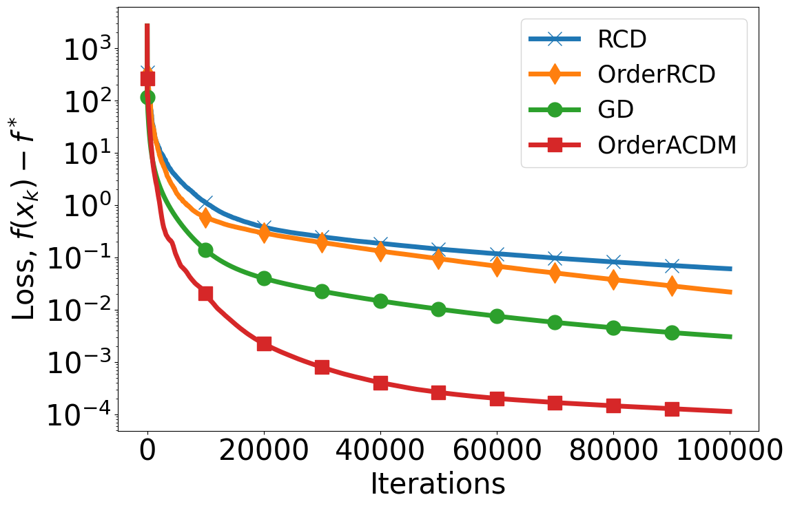
Figure 2: Comparison of the algorithms proposed in this paper with the SOTA non-accelerated first-order algorithms. Here we optimize $f(x)$ with the parameters: $d=100$ (dimensional of problem), $\Delta=0$ (maximum noise level in the Order Oracle).

The optimization problem (1) has a standard quadratic form:

$$\min_{x\in\mathbb{R}^{d}}f(x):=\frac{1}{2}\left\langle x,Ax\right\rangle-\left\langle b,x\right\rangle+c,$$

where $A\in\mathbb{R}^{d\times d}$, $b\in\mathbb{R}^{d}$, and $c\in\mathbb{R}$. We use a uniform distribution ($\alpha=0$) to choose the active coordinate, then the distribution (4) has the following form: $p_{0}(i)=1/d$. For such a problem, the assumptions of $L$-Coordinate-Lipschitz smoothness (Assumption 1.1) and $\mu_{1-\alpha}$-strong convexity (Assumption 1.2) are satisfied, where $L_{i}=A_{ii}$. In all experiments, we employ the golden ratio method (GRM) to solve the linear search problem with a precision of ${\epsilon=10^{-8}}$.

In Figure 2, we compare the convergence random coordinate descent with order oracle (OrderRCD) and accelerated coordinate descent method with order oracle (OrderACDM) with the SOTA non-accelerated algorithms: random coordinate descent (RCD) from Nesterov (2012), as well as gradient descent (GD). Non-accelerated coordinate algorithms, both for first-order oracle (RCD) and for the new oracle concept (OrderRCD), are observed to lag behind gradient descent, confirming our theoretical derivations in Section 3. Interestingly, the random coordinate descent with order oracle even outperforms its first-order counterpart, despite the limitations associated with oracle usage (only Order Oracle (2) available). This observation can be attributed to the adaptiveness of Algorithm 1, as OrderRCD employs an exact step in the steepest descent direction obtained using the golden ratio method (GRM) at each iteration. Additionally, we can observe perhaps the most significant result demonstrated in Figure 2: acceleration in the new oracle concept (2) exists! We see that accelerated coordinate descent method with order oracle outpaces the convergence speed of all non-accelerated algorithms, including first-order coordinate (RCD) and full-gradient (GD) methods. In this experiment, OrderACDM was implemented using the method described in Algorithm 2 with $\zeta_{k}=0$ (i.e., with one golden ratio method); RCD and GD used a constant step size, specifically $1/L_{i}$ and $1/L$.

In Figure 4, we investigate effect of adversarial noise $\delta(x,y)$ from the new oracle concept (2) on a random coordinate descent with order oracle (OrderRCD). We used ($\delta(x,y)=\Delta\cdot\cos{x}\cdot\sin{y}$) as the adversarial deterministic noise, where $\Delta$ (s.t. $|\delta(x,y)|\leq\Delta$) is the maximum noise level. In Figure 4, we see that the adversarial noise justifies its name as it accumulates over iterations. In addition, we observe that the convergence of the non-accelerated coordinate method depends directly on the maximum noise level $\Delta$, namely, the lower the noise level, the more accurately the algorithm converges. And finally we see that our theoretical results from Section 3 are confirmed, which indicate that the asymptote to which the algorithm converges can be controlled by the maximum noise level $\Delta$, for example, in this case, when $\alpha=0$, the condition for achieving the desired accuracy $\varepsilon$ looks as follows: ${\Delta\leq\mu_{1-\alpha}\varepsilon/d}$. Or we can rephrase this condition: the OrderRCD has a linear convergence rate to the asymptote depending on level noise $\Delta$.

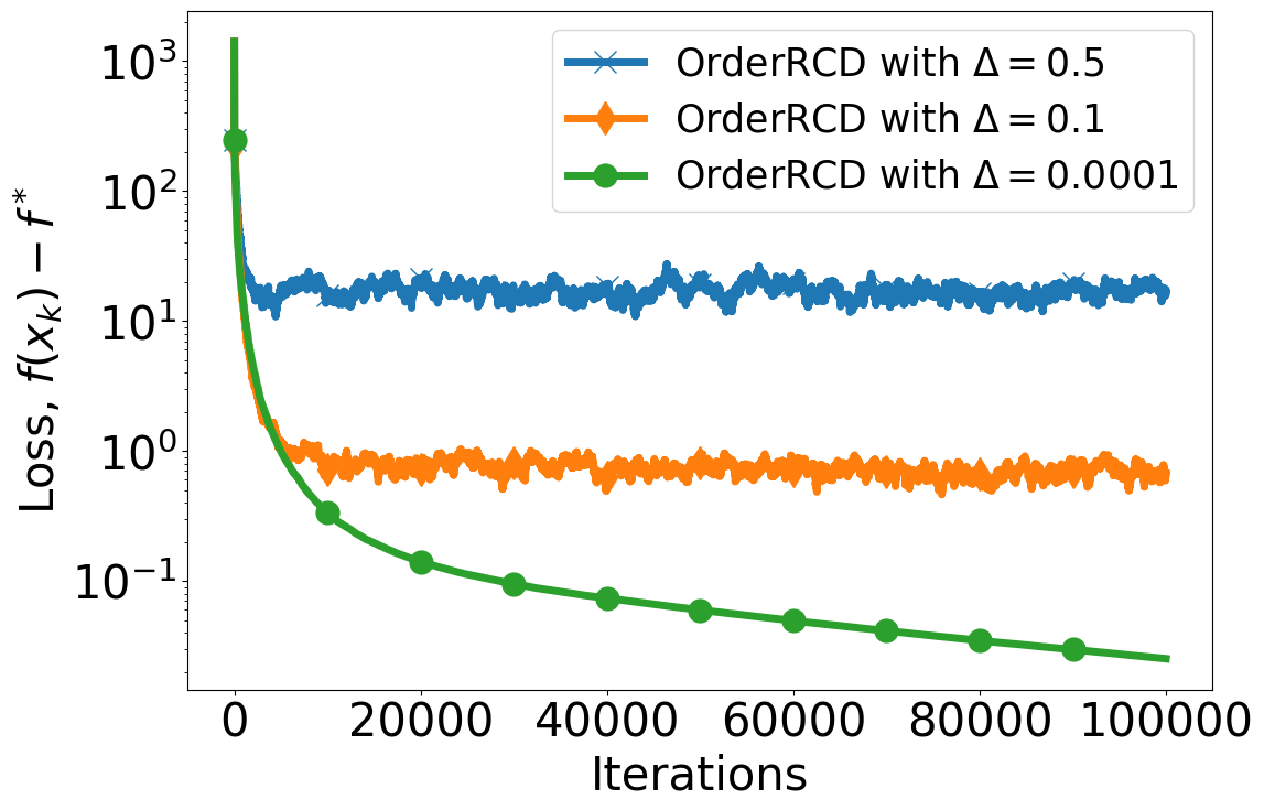
Figure 3: Effects of adversarial noise from the Order Oracle (2) on the convergence of random coordinate descent (OrderRCD). Here we optimize $f(x)$ with the parameters: $d=100$ (dimensional of problem), $\Delta=\{0.5,0.1,0.0001\}$ (maximum noise level).

02

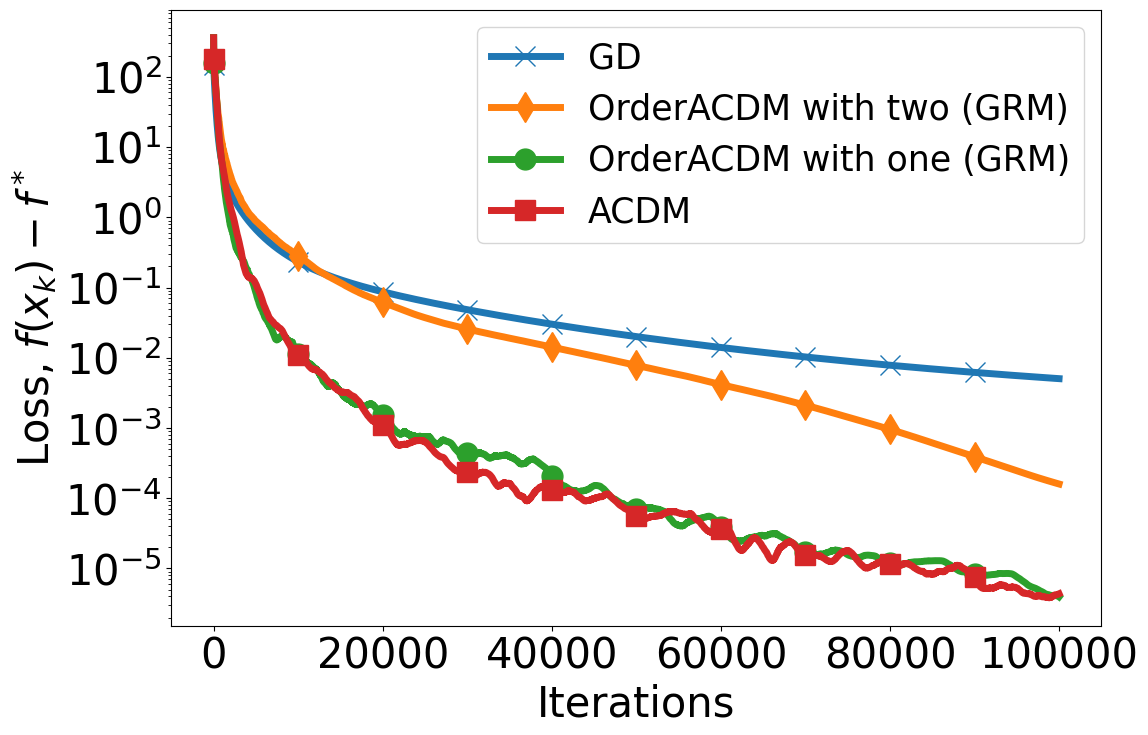
Figure 4: Effect of the second of golden ratio method on the convergence of accelerated coordinate descent with order oracle. Here we optimize $f(x)$ with the parameters: $d=100$ (dimensional of problem), $\Delta=0$ (maximum noise level in the Order Oracle).

In Figure 4, we illustrate the advantage of employing Algorithm 2 with one method of line search ($\zeta_{k}=0$). We can observe that the method proposed in Section 4, the accelerated coordinate descent with order oracle (OrderACDM with two (GRM)), indeed qualifies as accelerated (thus affirming the theoretical findings of Section 4) as it outperforms gradient descent (GD), which can be considered a boundary between non-accelerated and accelerated coordinate methods. However, this algorithm significantly lags behind the accelerated coordinate descent method (ACDM, Nesterov & Stich, 2017). The reason may be the delayed momentum effect caused by using the golden ratio method (GRM) a second time (see line 10 of Algorithm 2). Addressing this may involve utilizing the golden section method only once per iteration in Algorithm 2 (that is, substitute $\zeta_{k}=0$ into line 10). Indeed, we observe that when using the golden section method once per iteration in Algorithm 2, the OrderACDM enhances convergence rate and does not fall behind its first-order counterpart (ACDM) which confirms our theoretical results. That is why we recommend to utilize in practice accelerated coordinate descent method with order oracle (OrderACDM, see Algorithm 2) with only one the golden ratio method (GRM) per iteration.

7 Conclusion

We introduced a new oracle concept (2) that offers a more realistic representation compared to traditional zero-order oracles. Our approach, utilizing the Order Oracle for gradient-free algorithms, has demonstrated effectiveness across both non-accelerated and accelerated methods, which could be independently significant. The convergence guarantees of OrderRCD (in non-convex, convex, and strongly convex cases) and OrderACDM (in the strongly convex case) were theoretically established and validated through numerical experiments. Practical recommendations for implementing the algorithms were provided. Overall, we believe our work has opened up promising avenues in black-box optimization (and not only), made accessible through the Order Oracle.

Appendix A Auxiliary Results

In this section we provide auxiliary materials that are used in the proof of Theorems.

A.1 Basic inequalities and assumptions

Basic inequalities.

For all $a,b\in\mathbb{R}^{d}$ ($d\geq 1$) the following equality holds:

$$\|a\|^{2}+\|b\|^{2}=2\left\langle a,b\right\rangle+\|a-b\|^{2},$$ (8)

$$\left\langle a,b\right\rangle\leq\|a\|\cdot\|b\|.$$ (9)

Coordinate-Lipschitz-smoothness.

Throughout this paper, we assume that the smoothness condition (Assumption 1.1) is satisfied. This inequality can be represented in the equivalent form:

$$f(x+h\mathbf{e}_{i})\leq f(x)+h\nabla_{i}f(x)+\frac{L_{i}h^{2}}{2},$$ (10)

where $L_{1},L_{2},...,L_{d}>0$ for any $i\in[d],x\in\mathbb{R}^{d}$ and $h\in\mathbb{R}$.

Lipschitz-smoothness.

To prove Theorem 4.1, we additionally assume $L_{[1-\alpha]}$-smoothness w.r.t. the norm $\left\|\cdot\right\|_{[1-\alpha]}$:

$$f(y)\leq f(x)+\left\langle\nabla f(x),y-x\right\rangle+\frac{L_{[1-\alpha]}}{2}\left\|y-x\right\|_{[1-\alpha]}^{2},\quad\forall x,y\in\mathbb{R}^{d}.$$ (11)

A.2 The Golden Ratio Method (GRM)

Algorithms 1 and 2, presented in Section 3 and 4, respectively, use the Golden Ratio Method (GRM) at least once per iteration. This method utilizes the oracle concept (2) proposed in this paper and has the following form (See Algorithm 3).

1:  Input: Interval $[a,b]$

2:  Initialization: Choose constants $\epsilon>0$ (desired accuracy), put the constant $\rho=\frac{\sqrt{5}-1}{2}$

3:  $y\leftarrow a+(1-\rho)(b-a)$

4:  $z\leftarrow a+\rho(b-a)$

5:  while $b-a>\epsilon$ do

6:     if $\phi(y,z)=-1$ then

7:        $b\leftarrow z$

8:        $z\leftarrow y$

9:        $y\leftarrow a+(1-\rho)(b-a)$

10:     else

11:        $a\leftarrow y$

12:        $y\leftarrow z$

13:        $z\leftarrow a+\rho(b-a)$

14:     end if

15:  end while

16:  Return: $\frac{a+b}{2}$

Algorithm 3 Golden Ratio Method (GRM)

We utilize the Golden Ratio Method to find a solution to the following one-dimensional problem:

$$\eta_{k}=\operatorname*{arg\,min}_{\eta\in\mathbb{R}}f(x_{k}+\eta\mathbf{e}_{i_{k}}).$$

Further, we derive the following corollaries from the solution of this problem:

• In the scenario when the Order Oracle (2) is not subjected to an adversarial noise ($\Delta=0$), we observe the following:

  $$f(x_{k}+\eta_{k}\mathbf{e}_{i_{k}})\leq f(x_{k}+\eta\mathbf{e}_{i_{k}}),\quad\quad\quad\forall\eta\in\mathbb{R}.$$ (12)

• In the scenario when the Order Oracle (2) is not subjected to an adversarial noise ($\Delta>0$) we assume the worst case:

  $$f(x_{k}+\eta_{k}\mathbf{e}_{i_{k}})\leq f(x_{k}+\eta\mathbf{e}_{i_{k}})+\Delta,\quad\quad\quad\forall\eta\in\mathbb{R}.$$ (13)

In this final corollary, we consider the scenario where adversarial noise accumulates over iterations, resulting in the following observation: the golden ratio method converges towards the $\Delta$ asymptote.

Appendix B Proof of Convergence for Non-Accelerated Algorithm 1

In this section, we furnish the omitted proofs for the theorems presented in Section 3.

B.1 Proof of Theorem 3.1

From Assumption 1.1 we obtain:

$$f\left(x_{k}+\eta_{k}\mathbf{e}_{i_{k}}\right)-f(x_{k}) \overset{\eqref{eq:coll_with_noise}}{\leq}f\left(x_{k}-\frac{1}{L_{i_{k}}}\nabla_{i_{k}}f(x_{k})\mathbf{e}_{i_{k}}\right)-f(x_{k})+\Delta$$

$$\overset{\eqref{eq:ass_smooth}}{\leq}-\frac{1}{L_{i_{k}}}(\nabla_{i_{k}}f(x_{k}))^{2}+\frac{1}{2L_{i_{k}}}(\nabla_{i_{k}}f(x_{k}))^{2}+\Delta$$

$$=-\frac{1}{2L_{i_{k}}}(\nabla_{i_{k}}f(x_{k}))^{2}+\Delta,$$ (14)

where $\eta_{k}=\operatorname*{arg\,min}_{\eta\in\mathbb{R}}f(x_{k}+\eta\mathbf{e}_{i_{k}})$. We use this as follows:

$$\mathbb{E}\left[f(x_{k+1})\right]-f(x_{k}) =\mathbb{E}\left[f\left(x_{k}+\eta_{k}\mathbf{e}_{i_{k}}\right)\right]-f(x_{k})$$

$$\overset{\eqref{eq:distibution}}{=}\sum_{i=1}^{d}p_{\alpha}(i)\left(f\left(x_{k}+\eta_{k}\mathbf{e}_{i_{k}}\right)-f(x_{k})\right)$$

$$\overset{\eqref{eq:nonconv_1}}{\leq}-\sum_{i=1}^{d}p_{\alpha}(i)\frac{1}{2L_{i}}(\nabla_{i}f(x_{k}))^{2}+\sum_{i=1}^{d}p_{\alpha}(i)\Delta$$

$$=-\frac{1}{2S_{\alpha}}\left(\left\|\nabla f(x_{k})\right\|_{[1-\alpha]}^{*}\right)^{2}+\Delta.$$

Rearranging the terms and summing over all $k$, we have

$$\sum_{k=0}^{N-1}\frac{1}{2S_{\alpha}}\left(\left\|\nabla f(x_{k})\right\|_{[1-\alpha]}^{*}\right)^{2} \leq\sum_{k=0}^{N-1}\left(F_{k}-F_{k+1}\right)+\sum_{k=0}^{N-1}\Delta$$

$$\leq F_{0}+F_{N}+N\Delta$$

$$\leq F_{0}+N\Delta,$$

where $F_{k}=\mathbb{E}\left[f(x_{k})\right]-f(x^{*})$.

Dividing both sides by number of iterations $N$, we obtain the convergence rate for the non-convex case:

$$\frac{1}{N}\sum_{k=0}^{N-1}\left(\left\|\nabla f(x_{k})\right\|_{[1-\alpha]}^{*}\right)^{2} \leq\frac{2S_{\alpha}}{N}F_{0}+2S_{\alpha}\Delta.$$

This convergence results imply the existence of a point $k\in[N]$ where holds true:

$$\left(\left\|\nabla f(x_{k})\right\|_{[1-\alpha]}^{*}\right)^{2}\leq\mathcal{O}\left(\frac{S_{\alpha}F_{0}}{N}+S_{\alpha}\Delta\right).$$

Then, achieving the desired accuracy $\varepsilon$, where $\left\|\nabla f(x_{k})\right\|_{[1-\alpha]}^{*}\leq\varepsilon$, requires

$$N=\mathcal{O}\left(\frac{S_{\alpha}F_{0}}{\varepsilon^{2}}\right),\quad\quad\quad T=\tilde{\mathcal{O}}\left(\frac{S_{\alpha}F_{0}}{\varepsilon^{2}}\right)$$

iterations and oracle calls respectively, provided the maximum noise does not exceed $\Delta\leq\varepsilon^{2}/S_{\alpha}.$

B.2 Proof of Theorem 3.2

From Assumption 1.1 we obtain:

$$f\left(x_{k}+\eta_{k}\mathbf{e}_{i_{k}}\right)-f(x_{k}) \overset{\eqref{eq:coll_with_noise}}{\leq}f\left(x_{k}-\frac{1}{L_{i_{k}}}\nabla_{i_{k}}f(x_{k})\mathbf{e}_{i_{k}}\right)-f(x_{k})+\Delta$$

$$\overset{\eqref{eq:ass_smooth}}{\leq}-\frac{1}{L_{i_{k}}}(\nabla_{i_{k}}f(x_{k}))^{2}+\frac{1}{2L_{i_{k}}}(\nabla_{i_{k}}f(x_{k}))^{2}+\Delta$$

$$=-\frac{1}{2L_{i_{k}}}(\nabla_{i_{k}}f(x_{k}))^{2}+\Delta,$$ (15)

where $\eta_{k}=\operatorname*{arg\,min}_{\eta\in\mathbb{R}}f(x_{k}+\eta\mathbf{e}_{i_{k}})$. We use this as follows:

$$\mathbb{E}\left[f(x_{k+1})\right]-f(x_{k}) =\mathbb{E}\left[f\left(x_{k}+\eta_{k}\mathbf{e}_{i_{k}}\right)\right]-f(x_{k})$$

$$\overset{\eqref{eq:distibution}}{=}\sum_{i=1}^{d}p_{\alpha}(i)\left(f\left(x_{k}+\eta_{k}\mathbf{e}_{i_{k}}\right)-f(x_{k})\right)$$

$$\overset{\eqref{eq:conv_1}}{\leq}-\sum_{i=1}^{d}p_{\alpha}(i)\frac{1}{2L_{i}}(\nabla_{i}f(x_{k}))^{2}+\sum_{i=1}^{d}p_{\alpha}(i)\Delta$$

$$=-\frac{1}{2S_{\alpha}}\left(\left\|\nabla f(x_{k})\right\|_{[1-\alpha]}^{*}\right)^{2}+\Delta.$$ (16)

Denote $F_{k}=\mathbb{E}\left[f(x_{k})\right]-f(x^{*})$. Note that the above calculation can be used to show $f(x_{k+1})\leq f(x_{k})$, then we have

$$F_{k} \overset{\text{\char 172}}{\leq}\left\langle\nabla f(x_{k}),x_{k}-x^{*}\right\rangle$$

$$\overset{\eqref{eq:scalar_product_bound}}{\leq}\left\|x_{k}-x^{*}\right\|_{[1-\alpha]}\left\|\nabla f(x_{k})\right\|_{[1-\alpha]}^{*}$$

$$\leq R_{[1-\alpha]}\left\|\nabla f(x_{k})\right\|_{[1-\alpha]}^{*},$$ (17)

where in ① we used Assumption 1.2 with $\mu_{1-\alpha}=0$, and $R_{[1-\alpha]}=\sup_{x\in\mathbb{R}^{d}:f(x)\leq f(x_{0})}\left\|x-x^{*}\right\|_{[1-\alpha]}$.

Then substituting (17) into (16) we obtain:

$$F_{k+1}\leq F_{k}-\frac{1}{2S_{\alpha}R^{2}_{[1-\alpha]}}F_{k}^{2}+\Delta.$$

Rewriting this inequality, we obtain:

$$\frac{1}{2S_{\alpha}R^{2}_{[1-\alpha]}}F_{k}^{2}\leq F_{k}-F_{k+1}+\Delta.$$

Next, we divide both sides by $F_{k+1}F_{k}$:

$$\frac{1}{2S_{\alpha}R^{2}_{[1-\alpha]}}\cdot\frac{F_{k}}{F_{k+1}}\leq\frac{1}{F_{k+1}}-\frac{1}{F_{k}}+\frac{\Delta}{F_{k+1}F_{k}}.$$

Using the fact that $\frac{1}{2S_{\alpha}R^{2}_{[1-\alpha]}}\leq\frac{1}{2S_{\alpha}R^{2}_{[1-\alpha]}}\frac{F_{k}}{F_{k+1}}$ we obtain the following:

$$\frac{1}{2S_{\alpha}R^{2}_{[1-\alpha]}}\leq\frac{1}{F_{k+1}}-\frac{1}{F_{k}}+\frac{\Delta}{F_{k+1}F_{k}}.$$

When summing over all $k$

$$\sum_{k=0}^{N-1}\frac{1}{2S_{\alpha}R^{2}_{[1-\alpha]}}\leq\sum_{k=0}^{N-1}\left(\frac{1}{F_{k+1}}-\frac{1}{F_{k}}\right)+\sum_{k=0}^{N-1}\frac{\Delta}{F_{k+1}F_{k}},$$

we get:

$$N\frac{1}{2S_{\alpha}R^{2}_{[1-\alpha]}} \leq\frac{1}{F_{N}}-\frac{1}{F_{0}}+\frac{N\Delta}{F_{N}F_{N-1}}$$

$$\leq\frac{1}{F_{N}}+\frac{N\Delta}{F_{N}F_{N-1}}.$$

Taking into account the fact that $F_{N-1}=\mathbb{E}\left[f(x_{N-1})\right]-f(x^{*})\geq\varepsilon$ and rewriting the expression we obtain the convergence rate for the convex case:

$$\mathbb{E}\left[f(x_{N})\right]-f(x^{*})\leq\frac{2S_{\alpha}R^{2}_{[1-\alpha]}}{N}+\frac{2S_{\alpha}R^{2}_{[1-\alpha]}}{\varepsilon}\Delta.$$

Then, achieving the desired accuracy $\varepsilon$, where $\mathbb{E}\left[f(x_{N})\right]-f(x^{*})\leq\varepsilon$, requires

$$N=\mathcal{O}\left(\frac{S_{\alpha}R^{2}_{[1-\alpha]}}{\varepsilon}\right),\quad\quad\quad T=\tilde{\mathcal{O}}\left(\frac{S_{\alpha}R^{2}_{[1-\alpha]}}{\varepsilon}\right)$$

iterations and oracle calls respectively, provided the maximum noise does not exceed $\Delta\leq\varepsilon^{2}/(S_{\alpha}R^{2}_{[1-\alpha]}).$

B.3 Proof of Theorem 3.3

From Assumption 1.1 we obtain:

$$f\left(x_{k}+\eta_{k}\mathbf{e}_{i_{k}}\right)-f(x_{k}) \overset{\eqref{eq:coll_with_noise}}{\leq}f\left(x_{k}-\frac{1}{L_{i_{k}}}\nabla_{i_{k}}f(x_{k})\mathbf{e}_{i_{k}}\right)-f(x_{k})+\Delta$$

$$\overset{\eqref{eq:ass_smooth}}{\leq}-\frac{1}{L_{i_{k}}}(\nabla_{i_{k}}f(x_{k}))^{2}+\frac{1}{2L_{i_{k}}}(\nabla_{i_{k}}f(x_{k}))^{2}+\Delta$$

$$=-\frac{1}{2L_{i_{k}}}(\nabla_{i_{k}}f(x_{k}))^{2}+\Delta,$$ (18)

where $\eta_{k}=\operatorname*{arg\,min}_{\eta\in\mathbb{R}}f(x_{k}+\eta\mathbf{e}_{i_{k}})$. We use this as follows:

$$\mathbb{E}\left[f(x_{k+1})\right]-f(x_{k}) =\mathbb{E}\left[f\left(x_{k}+\eta_{k}\mathbf{e}_{i_{k}}\right)\right]-f(x_{k})$$

$$\overset{\eqref{eq:distibution}}{=}\sum_{i=1}^{d}p_{\alpha}(i)\left(f\left(x_{k}+\eta_{k}\mathbf{e}_{i_{k}}\right)-f(x_{k})\right)$$

$$\overset{\eqref{eq:sc_1}}{\leq}-\sum_{i=1}^{d}p_{\alpha}(i)\frac{1}{2L_{i}}(\nabla_{i}f(x_{k}))^{2}+\sum_{i=1}^{d}p_{\alpha}(i)\Delta$$

$$=-\frac{1}{2S_{\alpha}}\left(\left\|\nabla f(x_{k})\right\|_{[1-\alpha]}^{*}\right)^{2}+\Delta.$$ (19)

By strong convexity, we have

$$f(x_{k})-f(x^{*}) \overset{\text{\char 172}}{\leq}\left\langle\nabla f(x_{k}),x_{k}-x^{*}\right\rangle-\frac{\mu_{1-\alpha}}{2}\left\|x_{k}-x^{*}\right\|_{[1-\alpha]}$$

$$\overset{\eqref{eq:scalar_product_bound}}{\leq}\left\|\nabla f(x_{k})\right\|_{[1-\alpha]}^{*}\cdot\left\|x_{k}-x^{*}\right\|_{[1-\alpha]}-\frac{\mu_{1-\alpha}}{2}\left\|x_{k}-x^{*}\right\|_{[1-\alpha]}$$

$$\leq\frac{1}{\mu_{1-\alpha}}\left(\left\|\nabla f(x_{k})\right\|_{[1-\alpha]}^{*}\right)^{2},$$

where in ① we used Assumption 1.2 with $\mu_{1-\alpha}>0$. Then, using this inequality in (19) we have

$$\mathbb{E}\left[f(x_{k+1})\right]-f(x^{*})\leq\left(1-\frac{\mu_{1-\alpha}}{2S_{\alpha}}\right)\left(f(x_{k})-f(x^{*})\right)+\Delta.$$

Applying recursion we obtain a linear convergence rate:

$$\mathbb{E}\left[f(x_{N})\right]-f(x^{*})\leq\left(1-\frac{\mu_{1-\alpha}}{2S_{\alpha}}\right)^{N}\left(f(x_{0})-f(x^{*})\right)+\frac{2S_{\alpha}\Delta}{\mu_{1-\alpha}}.$$

Then, achieving the desired accuracy $\varepsilon$, where $\mathbb{E}\left[f(x_{N})\right]-f(x^{*})\leq\varepsilon$, requires

$$N=\mathcal{O}\left(\frac{S_{\alpha}}{\mu_{1-\alpha}}\log\frac{1}{\varepsilon}\right),\quad\quad\quad T=\tilde{\mathcal{O}}\left(\frac{S_{\alpha}}{\mu_{1-\alpha}}\log\frac{1}{\varepsilon}\right)$$

iterations and oracle calls respectively, provided the maximum noise does not exceed $\Delta\leq\mu_{1-\alpha}\varepsilon/S_{\alpha}.$

Appendix C Proof of Convergence for Accelerated Algorithm 2

Denote $\omega_{k}=(1-\beta_{k})z_{k}+\beta_{k}y_{k}$. Then

$$y_{k}=\frac{(1-\alpha_{k})x_{k}}{1-\alpha_{k}\beta_{k}}+\frac{\alpha_{k}(1-\beta_{k})}{1-\alpha_{k}\beta_{k}}\cdot\frac{\omega_{k}-\beta_{k}y_{k}}{1-\beta_{k}}=\frac{(1-\alpha_{k})x_{k}+\alpha_{k}\omega_{k}}{1-\alpha_{k}\beta_{k}}-\frac{\alpha_{k}\beta_{k}y_{k}}{1-\alpha_{k}\beta_{k}}.$$

Thus, in method we have the following representation:

$$y_{k}=(1-\alpha_{k})x_{k}+\alpha_{k}\omega_{k}.$$ (20)

Let the solution of initial problem denote $x^{*}=x_{*}=\operatorname*{arg\,min}_{x\in\mathbb{R}^{d}}f(x)$, then from Assumption 1.1 we obtain:

$$\frac{2L_{i_{k}}^{\alpha}a_{k+1}^{2}}{B^{2}_{k+1}p^{2}_{\beta}(i_{k})} \left(f(\underbrace{y_{k}+\eta_{k}\mathbf{e}_{i_{k}}}_{x_{k+1}})-f(y_{k})\right)\overset{\eqref{eq:col_without_noise}}{\leq}\frac{2L_{i_{k}}^{\alpha}a_{k+1}^{2}}{B^{2}_{k+1}p^{2}_{\beta}(i_{k})}\left(f\left(y_{k}-\frac{1}{L_{i_{k}}}\nabla_{i_{k}}f(y_{k})\mathbf{e}_{i_{k}}\right)-f(y_{k})\right)$$

$$\overset{\eqref{eq:ass_smooth}}{\leq}-\frac{a_{k+1}^{2}}{L_{i_{k}}^{1-\alpha}B^{2}_{k+1}p^{2}_{\beta}(i_{k})}\left(\nabla_{i_{k}}f(y_{k})\right)^{2}\pm\left\|\omega_{k}-x_{*}\right\|_{[1-\alpha]}^{2}$$

$$=-L_{i_{k}}^{1-\alpha}\left[(\omega_{k}^{(i_{k})}-x_{*}^{(i_{k})})^{2}+\left(\frac{a_{k+1}}{L_{i_{k}}^{1-\alpha}B_{k+1}p_{\beta}(i_{k})}\nabla_{i_{k}}f(y_{k})\right)^{2}\right]-\sum_{i\neq i_{k}}L_{i}^{1-\alpha}(\omega_{k}^{(i)}-x_{*}^{(i)})^{2}$$

$$\quad\quad+\left\|\omega_{k}-x_{*}\right\|_{[1-\alpha]}^{2}$$

$$\overset{\eqref{eq:qudrat_raznosti}}{=}-L_{i_{k}}^{1-\alpha}\left[\left(\omega_{k}^{(i_{k})}-x_{*}^{(i_{k})}-\frac{a_{k+1}}{L_{i_{k}}^{1-\alpha}B_{k+1}p_{\beta}(i_{k})}\nabla_{i_{k}}f(y_{k})\right)^{2}+\frac{2a_{k+1}}{L_{i_{k}}^{1-\alpha}B_{k+1}p_{\beta}(i_{k})}\left\langle\nabla_{i_{k}}f(y_{k}),\omega_{k}^{(i_{k})}-x_{*}^{(i_{k})}\right\rangle\right]$$

$$\quad\quad-\sum_{i\neq i_{k}}L_{i}^{1-\alpha}(\omega_{k}^{(i)}-x_{*}^{(i)})^{2}+\left\|\omega_{k}-x_{*}\right\|_{[1-\alpha]}^{2}$$

$$=-\left\|\omega_{k}-\frac{a_{k+1}}{L_{i_{k}}^{1-\alpha}B_{k+1}p_{\beta}(i_{k})}\nabla_{i_{k}}f(y_{k})\mathbf{e}_{i_{k}}-x_{*}\right\|_{[1-\alpha]}^{2}+\left\|\omega_{k}-x_{*}\right\|_{[1-\alpha]}^{2}$$

$$\quad\quad-\frac{2a_{k+1}}{B_{k+1}p_{\beta}(i_{k})}\left\langle\nabla_{i_{k}}f(y_{k}),\omega_{k}^{(i_{k})}-x_{*}^{(i_{k})}\right\rangle+\frac{2}{\mu_{1-\alpha}}\left\langle\nabla f(x_{*}),z_{k+1}-x_{*}\right\rangle$$

$$\overset{\text{\char 172}}{\leq}-\left\|\omega_{k}-\frac{a_{k+1}}{L_{i_{k}}^{1-\alpha}B_{k+1}p_{\beta}(i_{k})}\nabla_{i_{k}}f(y_{k})\mathbf{e}_{i_{k}}-x_{*}\right\|_{[1-\alpha]}^{2}+\left\|\omega_{k}-x_{*}\right\|_{[1-\alpha]}^{2}$$

$$\quad\quad-\frac{2a_{k+1}}{B_{k+1}p_{\beta}(i_{k})}\left\langle\nabla_{i_{k}}f(y_{k}),\omega_{k}^{(i_{k})}-x_{*}^{(i_{k})}\right\rangle-\left\|z_{k+1}-x_{*}\right\|_{[1-\alpha]}^{2}+\frac{2}{\mu_{1-\alpha}}\left(f(z_{k+1})-f(x_{*})\right)$$

$$\overset{\eqref{eq:ass_norm_smooth}}{\leq}-\left\|z_{k+1}-x_{*}\right\|_{[1-\alpha]}^{2}+\left\|\omega_{k}-x_{*}\right\|_{[1-\alpha]}^{2}-\frac{2a_{k+1}}{B_{k+1}p_{\beta}(i_{k})}\left\langle\nabla_{i_{k}}f(y_{k}),\omega_{k}^{(i_{k})}-x_{*}^{(i_{k})}\right\rangle$$

$$\quad\quad+\frac{2}{\mu_{1-\alpha}}\left[f(z_{k+1})-f(x_{*})\right]+\frac{2}{L_{1-\alpha}}\left[f(x_{*})-f\left(\omega_{k}-\frac{a_{k+1}}{L_{i_{k}}^{1-\alpha}B_{k+1}p_{\beta}(i_{k})}\nabla_{i_{k}}f(y_{k})\mathbf{e}_{i_{k}}\right)\right]$$

$$\quad\quad-\frac{2}{L_{1-\alpha}}\left\langle\nabla f(x_{*}),\omega_{k}-\frac{a_{k+1}}{L_{i_{k}}^{1-\alpha}B_{k+1}p_{\beta}(i_{k})}\nabla_{i_{k}}f(y_{k})\mathbf{e}_{i_{k}}-x_{*}\right\rangle$$

$$\leq-\left\|z_{k+1}-x_{*}\right\|_{[1-\alpha]}^{2}+\left\|\omega_{k}-x_{*}\right\|_{[1-\alpha]}^{2}-\frac{2a_{k+1}}{B_{k+1}p_{\beta}(i_{k})}\left\langle\nabla_{i_{k}}f(y_{k}),\omega_{k}^{(i_{k})}-x_{*}^{(i_{k})}\right\rangle$$

$$\quad\quad+\frac{2}{\sigma_{1-\alpha}}\left[f(z_{k+1})-f(x_{*})+f(x_{*})-f\left(\omega_{k}-\frac{a_{k+1}}{L_{i_{k}}^{1-\alpha}B_{k+1}p_{\beta}(i_{k})}\nabla_{i_{k}}f(y_{k})\mathbf{e}_{i_{k}}\right)\right]$$

$$\overset{\eqref{eq:col_without_noise}}{\leq}-\left\|z_{k+1}-x_{*}\right\|_{[1-\alpha]}^{2}+\left\|\omega_{k}-x_{*}\right\|_{[1-\alpha]}^{2}-\frac{2a_{k+1}}{B_{k+1}p_{\beta}(i_{k})}\left\langle\nabla_{i_{k}}f(y_{k}),\omega_{k}^{(i_{k})}-x_{*}^{(i_{k})}\right\rangle,$$ (21)

where in ① we used Assumption 1.2 with $\mu_{1-\alpha}>0$.

Denote $r_{k}^{2}=\left\|z_{k}-x_{*}\right\|_{[1-\alpha]}^{2}$ and $\omega_{k}=(1-\beta_{k})z_{k}+\beta_{k}y_{k}$, then due to convexity of the norm function it follows:

$$\left\|\omega_{k}-x_{*}\right\|_{[1-\alpha]}^{2}\leq(1-\beta_{k})\left\|z_{k}-x_{*}\right\|_{[1-\alpha]}^{2}+\beta_{k}\left\|y_{k}-x_{*}\right\|_{[1-\alpha]}^{2}.$$ (22)

Substituting (22) into (21) we obtain

$$B_{k+1}r^{2}_{k+1} \overset{\eqref{eq:eq2}}{\leq}(1-\beta_{k})B_{k+1}r^{2}_{k}+\beta_{k}B_{k+1}\left\|y_{k}-x_{*}\right\|_{[1-\alpha]}^{2}$$

$$\quad\quad-\frac{2a_{k+1}}{p_{\beta}(i_{k})}\left\langle\nabla_{i_{k}}f(y_{k})\mathbf{e}_{i_{k}},\omega_{k}^{i_{k}}-x_{*}^{i_{k}}\right\rangle+\frac{2L_{i_{k}}^{\alpha}a_{k+1}^{2}}{B_{k+1}p^{2}_{\beta}(i_{k})}\left(f(y_{k})-f(x_{k+1})\right)$$

$$\overset{\text{\char 172}}{\leq}B_{k}r^{2}_{k}+\beta_{k}B_{k+1}\left\|y_{k}-x_{*}\right\|_{[1-\alpha]}^{2}-\frac{2a_{k+1}}{p_{\beta}(i_{k})}\left\langle\nabla_{i_{k}}f(y_{k})\mathbf{e}_{i_{k}},\omega_{k}^{i_{k}}-x_{*}^{i_{k}}\right\rangle+\frac{2L_{i_{k}}^{\alpha}a_{k+1}^{2}}{B_{k+1}p^{2}_{\beta}(i_{k})}\left(f(y_{k})-f(x_{k+1})\right)$$

$$\overset{\eqref{eq:distibution}}{\leq}B_{k}r^{2}_{k}+\beta_{k}B_{k+1}\left\|y_{k}-x_{*}\right\|_{[1-\alpha]}^{2}-\frac{2a_{k+1}}{p_{\beta}(i_{k})}\left\langle\nabla_{i_{k}}f(y_{k})\mathbf{e}_{i_{k}},\omega_{k}^{i_{k}}-x_{*}^{i_{k}}\right\rangle+\frac{2L_{i_{k}}^{\alpha}a_{k+1}^{2}S_{\beta}^{2}}{B_{k+1}L_{i_{k}}^{2\beta}}\left(f(y_{k})-f(x_{k+1})\right)$$

$$\overset{\text{\char 173}}{=}B_{k}r^{2}_{k}+\beta_{k}B_{k+1}\left\|y_{k}-x_{*}\right\|_{[1-\alpha]}^{2}-\frac{2a_{k+1}}{p_{\beta}(i_{k})}\left\langle\nabla_{i_{k}}f(y_{k})\mathbf{e}_{i_{k}},\omega_{k}^{i_{k}}-x_{*}^{i_{k}}\right\rangle+\frac{2a_{k+1}^{2}S_{\beta}^{2}}{B_{k+1}}\left(f(y_{k})-f(x_{k+1})\right),$$

where in ① we use that $(1-\beta_{k})B_{k+1}=B_{k+1}-\sigma_{1-\alpha}a_{k+1}=B_{k}$, and in ② we use that $\alpha=2\beta$.

Note that $\mathbb{E}\left[f(x_{k+1})\right]=\sum_{i=1}^{d}p_{\beta}(i)f(x_{k+1})$. Therefore, taking expectation we obtain:

$$\mathbb{E}\left[B_{k+1}r^{2}_{k+1}\right] \leq B_{k}r^{2}_{k}+\beta_{k}B_{k+1}\left\|y_{k}-x_{*}\right\|_{[1-\alpha]}^{2}-\mathbb{E}\left[\frac{2a_{k+1}}{p_{\beta}(i_{k})}\left\langle\nabla_{i_{k}}f(y_{k})\mathbf{e}_{i_{k}},\omega_{k}^{i_{k}}-x_{*}^{i_{k}}\right\rangle\right]$$

$$\quad\quad+\frac{2a_{k+1}^{2}S_{\beta}^{2}}{B_{k+1}}\left(f(y_{k})-\mathbb{E}\left[f(x_{k+1})\right]\right)$$

$$\leq B_{k}r^{2}_{k}+\beta_{k}B_{k+1}\left\|y_{k}-x_{*}\right\|_{[1-\alpha]}^{2}-\sum_{i=1}^{d}p_{\beta}(i)\frac{2a_{k+1}}{p_{\beta}(i)}\left\langle\nabla_{i}f(y_{k})\mathbf{e}_{i},\omega_{k}^{i}-x_{*}^{i}\right\rangle$$

$$\quad\quad+\frac{2a_{k+1}^{2}S_{\beta}^{2}}{B_{k+1}}\left(f(y_{k})-\mathbb{E}\left[f(x_{k+1})\right]\right)$$

$$=B_{k}r^{2}_{k}+\beta_{k}B_{k+1}\left\|y_{k}-x_{*}\right\|_{[1-\alpha]}^{2}+2a_{k+1}\left\langle\nabla f(y_{k}),x_{*}-\omega_{k}\right\rangle+\frac{2a_{k+1}^{2}S_{\beta}^{2}}{B_{k+1}}\left(f(y_{k})-\mathbb{E}\left[f(x_{k+1})\right]\right).$$

Since $\omega_{k}\overset{\eqref{eq:y_k}}{=}y_{k}+\frac{1-\alpha_{k}}{\alpha_{k}}(y_{k}-x_{k})$, we obtain

$$2a_{k+1}\left\langle\nabla f(y_{k}),x_{*}-\omega_{k}\right\rangle =2a_{k+1}\left\langle\nabla f(y_{k}),x_{*}-y_{k}+\frac{1-\alpha_{k}}{\alpha_{k}}(x_{k}-y_{k})\right\rangle$$

$$\overset{\text{\char 172}}{\leq}2a_{k+1}\left(f(x_{*})-f(y_{k})\right)-a_{k+1}\sigma_{1-\alpha}\left\|x_{*}-y_{k}\right\|_{[1-\alpha]}^{2}$$

$$\quad\quad+2a_{k+1}\frac{1-\alpha_{k}}{\alpha_{k}}\left(f(x_{k})-f(y_{k})\right)$$

$$\overset{\text{\char 173}}{=}2a_{k+1}f(x_{*})-2A_{k+1}f(y_{k})+2A_{k}f(x_{k})-a_{k+1}\sigma_{1-\alpha}\left\|x_{*}-y_{k}\right\|_{[1-\alpha]}^{2},$$ (23)

where in ① we use Assumption 1.2 with $\mu_{1-\alpha}>0$ and in ② we use that $a_{k+1}\frac{1-\alpha_{k}}{\alpha_{k}}=a_{k+1}\frac{1-\frac{a_{k+1}}{A_{k+1}}}{\frac{a_{k+1}}{A_{k+1}}}=A_{k+1}-a_{k+1}=A_{k}$.

$$\mathbb{E}\left[B_{k+1}r^{2}_{k+1}\right] \leq B_{k}r^{2}_{k}+\beta_{k}B_{k+1}\left\|y_{k}-x_{*}\right\|_{[1-\alpha]}^{2}+2a_{k+1}\left\langle\nabla f(y_{k}),x_{*}-\omega_{k}\right\rangle+\frac{2a_{k+1}^{2}S_{\beta}^{2}}{B_{k+1}}\left(f(y_{k})-\mathbb{E}\left[f(x_{k+1})\right]\right)$$

$$\overset{\text{\char 172}}{=}B_{k}r^{2}_{k}+a_{k+1}\sigma_{1-\alpha}\left\|y_{k}-x_{*}\right\|_{[1-\alpha]}^{2}+2a_{k+1}\left\langle\nabla f(y_{k}),x_{*}-\omega_{k}\right\rangle+\frac{2a_{k+1}^{2}S_{\beta}^{2}}{B_{k+1}}\left(f(y_{k})-\mathbb{E}\left[f(x_{k+1})\right]\right)$$

$$\overset{\eqref{eq:eq3}}{\leq}B_{k}r_{k}^{2}+2a_{k+1}f(x_{*})-2A_{k+1}f(y_{k})+2A_{k}f(x_{k})\pm 2A_{k}f(x_{*})+\frac{2a_{k+1}^{2}S_{\beta}^{2}}{B_{k+1}}\left(f(y_{k})-\mathbb{E}\left[f(x_{k+1})\right]\right)$$

$$\overset{\text{\char 173}}{=}B_{k}r_{k}^{2}+2a_{k+1}f(x_{*})-2A_{k+1}f(y_{k})+2A_{k}f(x_{k})\pm 2A_{k}f(x_{*})+2A_{k+1}\left(f(y_{k})-\mathbb{E}\left[f(x_{k+1})\right]\right)$$

$$=B_{k}r_{k}^{2}-2A_{k+1}\left(\mathbb{E}\left[f(x_{k+1})\right]-f(x_{*})\right)+2A_{k}\left(f(x_{k})-f(x_{*})\right),$$

where in ① we use that $\beta_{k}=\frac{\sigma_{1-\alpha}a_{k+1}}{B_{l+1}}$, and in ② we use that $a^{2}_{k+1}S^{2}_{\beta}=A_{k+1}B_{k+1}$.

By summing over $k$ we obtain:

$$2\sum_{k=0}^{N-1}A_{k+1}\left(\mathbb{E}\left[f(x_{k+1})\right]-f(x_{*})\right)\leq 2\sum_{k=0}^{N-1}A_{k}\left(f(x_{k})-f(x_{*})\right)+\sum_{k=0}^{N-1}B_{k}r_{k}^{2}-\sum_{k=0}^{N-1}\mathbb{E}\left[B_{k+1}r^{2}_{k+1}\right].$$

$$2A_{N}\left(\mathbb{E}\left[f(x_{N})\right]-f(x_{*})\right)\leq 2A_{0}\left(f(x_{0})-f(x_{*})\right)+B_{0}r_{0}^{2}-\mathbb{E}\left[B_{N}r^{2}_{N}\right].$$

Using the known facts from Nesterov & Stich (2017) we can estimate the parameters $A_{N}$ and $B_{N}$:

$$A_{N} \geq\frac{1}{4\mu_{1-\alpha}}\left[(1+\gamma)^{N}-(1-\gamma)^{N}\right]^{2}$$

$$\geq\frac{1}{4\mu_{1-\alpha}}\left[(1+\gamma)^{N}-1\right]^{2}\geq\frac{1}{8\mu_{1-\alpha}}(1+\gamma)^{2N}\geq\frac{1}{8\mu_{1-\alpha}}(1+\gamma)^{N},$$

$$B_{N} \geq\frac{1}{4}\left[(1+\gamma)^{N}+(1-\gamma)^{N}\right]^{2},$$

where $\gamma=\frac{\sqrt{\mu_{1-\alpha}}}{2S_{\alpha/2}}$. Then using $A_{0}=0$ and $B_{0}=1$ we have

$$A_{N}\left(\mathbb{E}\left[f(x_{N})\right]-f(x_{*})\right) \leq 2A_{0}\left(f(x_{0})-f(x_{*})\right)+B_{0}r_{0}^{2}-B_{N}\mathbb{E}\left[r^{2}_{N}\right].$$

$$\overset{\text{\char 172}}{\leq}\frac{1}{\mu_{1-\alpha}}\left(f(x_{0})-f(x_{*})-\left\langle\nabla f(x_{*}),x_{0}-x_{*}\right\rangle\right)$$

$$=\frac{1}{\mu_{1-\alpha}}\left(f(x_{0})-f(x_{*})\right).$$

Let’s divide both parts by $A_{N}$, then we have the convergence rate for accelerated method

$$\mathbb{E}\left[f(x_{N})\right]-f(x_{*}) \leq\frac{1}{\mu_{1-\alpha}A_{N}}\left(f(x_{0})-f(x_{*})\right)$$

$$\leq 8(1+\gamma)^{-N}\left(f(x_{0})-f(x_{*})\right)$$

$$\leq 8(1-\gamma)^{N}\left(f(x_{0})-f(x_{*})\right)$$

$$=8\left(1-\frac{\sqrt{\mu_{1-\alpha}}}{2S_{\alpha/2}}\right)^{N}\left(f(x_{0})-f(x_{*})\right).$$

Then, achieving the desired accuracy $\varepsilon$, where $\mathbb{E}\left[f(x_{N})\right]-f(x^{*})\leq\varepsilon$, requires

$$N=\mathcal{O}\left(\frac{S_{\alpha/2}}{\sqrt{\mu_{1-\alpha}}}\log\frac{1}{\varepsilon}\right),\quad\quad\quad T=\tilde{\mathcal{O}}\left(\frac{S_{\alpha/2}}{\sqrt{\mu_{1-\alpha}}}\log\frac{1}{\varepsilon}\right)$$

iterations and oracle calls respectively.

Appendix D Description of the “Private Communication” Approach

In this section, we describe an approach provided in Nesterov et al. (2018) to create a more efficient algorithm for low-dimensional problems, compared to the gradient-based methods proposed in this paper, using only the Order Oracle (2).

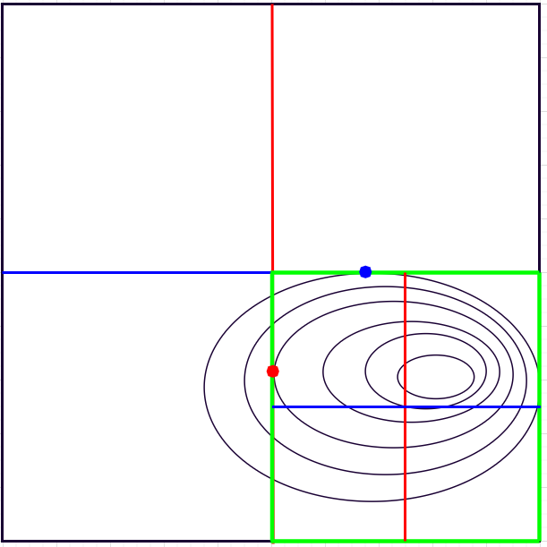
Figure 5: Schematic of algorithm

Consider the following method for solving the problem of minimizing a convex Lipschitz function (with Lipschitz constant $L$) on a square in $\mathbb{R}^{2}$ with side $R$. A horizontal line (blue line) is drawn through the center of the square. On the interval carved from the square of this line, with accuracy $\sim\varepsilon/\log(LR/\varepsilon)$ (by function) we solve the one-dimensional optimization (line search) problem. At the found point (blue point), the direction of the function gradient (which is determined via the Order Oracle) is calculated and it is determined in which of the two rectangles it “looks”; this rectangle is “discarded”. A vertical line (red line) is drawn through the center of the remaining rectangle, and on the segment carved by this line in the rectangle, also with accuracy $\sim\varepsilon/\log(LR/\varepsilon)$ (by function) solves the problem of one-dimensional optimization (line search) problem. At the found point (red point), the direction of the function gradient (which is determined via the Order Oracle) is calculated and it is determined in which of the two rectangles it “looks”; this rectangle is “discarded”. As a result of this procedure, the linear size of the original square is halved (green square). The schematic of the performance of the algorithm is shown in Figure 5.

Corollary D.1.

It is not difficult to show that after $\log(LR/\varepsilon)$ repetitions of such a procedure we can find with $\varepsilon$ accuracy (by function) the solution of the original problem.

References

• Agafonov et al. (2023) Agafonov, A., Kamzolov, D., Dvurechensky, P., Gasnikov, A., and Takáč, M. Inexact tensor methods and their application to stochastic convex optimization. Optimization Methods and Software, pp.  1–42, 2023.
• Agarwal et al. (2010) Agarwal, A., Dekel, O., and Xiao, L. Optimal algorithms for online convex optimization with multi-point bandit feedback. In Colt, pp.  28–40. Citeseer, 2010.
• Agarwal et al. (2011) Agarwal, A., Foster, D. P., Hsu, D. J., Kakade, S. M., and Rakhlin, A. Stochastic convex optimization with bandit feedback. Advances in Neural Information Processing Systems, 24, 2011.
• Ajalloeian & Stich (2020) Ajalloeian, A. and Stich, S. U. On the convergence of sgd with biased gradients. arXiv preprint arXiv:2008.00051, 2020.
• Akhavan et al. (2021) Akhavan, A., Pontil, M., and Tsybakov, A. Distributed zero-order optimization under adversarial noise. Advances in Neural Information Processing Systems, 34:10209–10220, 2021.
• Akhavan et al. (2022) Akhavan, A., Chzhen, E., Pontil, M., and Tsybakov, A. A gradient estimator via l1-randomization for online zero-order optimization with two point feedback. Advances in Neural Information Processing Systems, 35:7685–7696, 2022.
• Alacaoglu et al. (2023) Alacaoglu, A., Böhm, A., and Malitsky, Y. Beyond the golden ratio for variational inequality algorithms. Journal of Machine Learning Research, 24(172):1–33, 2023.
• Alashqar et al. (2023) Alashqar, B., Gasnikov, A., Dvinskikh, D., and Lobanov, A. Gradient-free federated learning methods with $l_{1}$ and $l_{2}$-randomization for non-smooth convex stochastic optimization problems. Computational Mathematics and Mathematical Physics, 63(9):1600–1653, 2023.
• Allen-Zhu et al. (2016) Allen-Zhu, Z., Qu, Z., Richtárik, P., and Yuan, Y. Even faster accelerated coordinate descent using non-uniform sampling. In International Conference on Machine Learning, pp.  1110–1119. PMLR, 2016.
• Anikin et al. (2015) Anikin, A., Dvurechensky, P., Gasnikov, A., Golov, A., Gornov, A., Maximov, Y., Mendel, M., and Spokoiny, V. Modern efficient numerical approaches to regularized regression problems in application to traffic demands matrix calculation from link loads. In Proceedings of International conference ITAS-2015, 2015.
• Asi et al. (2021) Asi, H., Feldman, V., Koren, T., and Talwar, K. Private stochastic convex optimization: Optimal rates in l1 geometry. In International Conference on Machine Learning, pp.  393–403. PMLR, 2021.
• Bach & Perchet (2016) Bach, F. and Perchet, V. Highly-smooth zero-th order online optimization. In Conference on Learning Theory, pp.  257–283. PMLR, 2016.
• Bansal et al. (2017) Bansal, S., Calandra, R., Xiao, T., Levine, S., and Tomlin, C. J. Goal-driven dynamics learning via bayesian optimization. In 2017 IEEE 56th Annual Conference on Decision and Control (CDC), pp.  5168–5173. IEEE, 2017.
• Belkin (2021) Belkin, M. Fit without fear: remarkable mathematical phenomena of deep learning through the prism of interpolation. Acta Numerica, 30:203–248, 2021.
• Belloni et al. (2015) Belloni, A., Liang, T., Narayanan, H., and Rakhlin, A. Escaping the local minima via simulated annealing: Optimization of approximately convex functions. In Conference on Learning Theory, pp.  240–265. PMLR, 2015.
• Bergstra & Bengio (2012) Bergstra, J. and Bengio, Y. Random search for hyper-parameter optimization. Journal of machine learning research, 13(2), 2012.
• Boyd & Vandenberghe (2004) Boyd, S. P. and Vandenberghe, L. Convex optimization. Cambridge university press, 2004.
• Bubeck et al. (2017) Bubeck, S., Lee, Y. T., and Eldan, R. Kernel-based methods for bandit convex optimization. In Proceedings of the 49th Annual ACM SIGACT Symposium on Theory of Computing, pp.  72–85, 2017.
• Bubeck et al. (2015) Bubeck, S. et al. Convex optimization: Algorithms and complexity. Foundations and Trends® in Machine Learning, 8(3-4):231–357, 2015.
• Chen et al. (2017) Chen, P.-Y., Zhang, H., Sharma, Y., Yi, J., and Hsieh, C.-J. Zoo: Zeroth order optimization based black-box attacks to deep neural networks without training substitute models. In Proceedings of the 10th ACM workshop on artificial intelligence and security, pp.  15–26, 2017.
• Choromanski et al. (2018) Choromanski, K., Rowland, M., Sindhwani, V., Turner, R., and Weller, A. Structured evolution with compact architectures for scalable policy optimization. In International Conference on Machine Learning, pp.  970–978. PMLR, 2018.
• Conn et al. (2009) Conn, A. R., Scheinberg, K., and Vicente, L. N. Introduction to derivative-free optimization. SIAM, 2009.
• Cutkosky & Mehta (2021) Cutkosky, A. and Mehta, H. High-probability bounds for non-convex stochastic optimization with heavy tails. Advances in Neural Information Processing Systems, 34:4883–4895, 2021.
• Dai et al. (2020) Dai, Z., Low, B. K. H., and Jaillet, P. Federated bayesian optimization via thompson sampling. Advances in Neural Information Processing Systems, 33:9687–9699, 2020.
• Duchi (2016) Duchi, J. Lecture notes for statistics 311/electrical engineering 377. URL: https://stanford. edu/class/stats311/Lectures/full notes. pdf. Last visited on, 2:23, 2016.
• Duchi et al. (2011) Duchi, J., Hazan, E., and Singer, Y. Adaptive subgradient methods for online learning and stochastic optimization. Journal of machine learning research, 12(7), 2011.
• Faw et al. (2022) Faw, M., Tziotis, I., Caramanis, C., Mokhtari, A., Shakkottai, S., and Ward, R. The power of adaptivity in sgd: Self-tuning step sizes with unbounded gradients and affine variance. In Conference on Learning Theory, pp.  313–355. PMLR, 2022.
• Fawzi et al. (2016) Fawzi, A., Moosavi-Dezfooli, S.-M., and Frossard, P. Robustness of classifiers: from adversarial to random noise. Advances in neural information processing systems, 29, 2016.
• Gao et al. (2018) Gao, J., Lanchantin, J., Soffa, M. L., and Qi, Y. Black-box generation of adversarial text sequences to evade deep learning classifiers. In 2018 IEEE Security and Privacy Workshops (SPW), pp.  50–56. IEEE, 2018.
• Gasnikov et al. (2022a) Gasnikov, A., Dvinskikh, D., Dvurechensky, P., Gorbunov, E., Beznosikov, A., and Lobanov, A. Randomized gradient-free methods in convex optimization. arXiv preprint arXiv:2211.13566, 2022a.
• Gasnikov et al. (2022b) Gasnikov, A., Novitskii, A., Novitskii, V., Abdukhakimov, F., Kamzolov, D., Beznosikov, A., Takac, M., Dvurechensky, P., and Gu, B. The power of first-order smooth optimization for black-box non-smooth problems. In International Conference on Machine Learning, pp.  7241–7265. PMLR, 2022b.
• Ghadimi & Lan (2013) Ghadimi, S. and Lan, G. Stochastic first-and zeroth-order methods for nonconvex stochastic programming. SIAM Journal on Optimization, 23(4):2341–2368, 2013.
• Glasgow et al. (2022) Glasgow, M. R., Yuan, H., and Ma, T. Sharp bounds for federated averaging (local sgd) and continuous perspective. In International Conference on Artificial Intelligence and Statistics, pp.  9050–9090. PMLR, 2022.
• Gorbunov et al. (2020) Gorbunov, E., Danilova, M., and Gasnikov, A. Stochastic optimization with heavy-tailed noise via accelerated gradient clipping. Advances in Neural Information Processing Systems, 33:15042–15053, 2020.
• Gurbuzbalaban et al. (2021) Gurbuzbalaban, M., Simsekli, U., and Zhu, L. The heavy-tail phenomenon in sgd. In International Conference on Machine Learning, pp.  3964–3975. PMLR, 2021.
• Hernández-Lobato et al. (2014) Hernández-Lobato, J. M., Hoffman, M. W., and Ghahramani, Z. Predictive entropy search for efficient global optimization of black-box functions. Advances in neural information processing systems, 27, 2014.
• Hodgkinson & Mahoney (2021) Hodgkinson, L. and Mahoney, M. Multiplicative noise and heavy tails in stochastic optimization. In International Conference on Machine Learning, pp.  4262–4274. PMLR, 2021.
• Huang et al. (2022) Huang, F., Gao, S., Pei, J., and Huang, H. Accelerated zeroth-order and first-order momentum methods from mini to minimax optimization. The Journal of Machine Learning Research, 23(1):1616–1685, 2022.
• Huang et al. (2023) Huang, F., Wu, X., and Hu, Z. Adagda: Faster adaptive gradient descent ascent methods for minimax optimization. In International Conference on Artificial Intelligence and Statistics, pp.  2365–2389. PMLR, 2023.
• Jiang et al. (2019) Jiang, B., Wang, H., and Zhang, S. An optimal high-order tensor method for convex optimization. In Conference on Learning Theory, pp.  1799–1801. PMLR, 2019.
• Karimi et al. (2016) Karimi, H., Nutini, J., and Schmidt, M. Linear convergence of gradient and proximal-gradient methods under the polyak-łojasiewicz condition. In Machine Learning and Knowledge Discovery in Databases: European Conference, ECML PKDD 2016, Riva del Garda, Italy, September 19-23, 2016, Proceedings, Part I 16, pp.  795–811. Springer, 2016.
• Kavis et al. (2022) Kavis, A., Levy, K. Y., and Cevher, V. High probability bounds for a class of nonconvex algorithms with adagrad stepsize. arXiv preprint arXiv:2204.02833, 2022.
• Kimiaei & Neumaier (2022) Kimiaei, M. and Neumaier, A. Efficient unconstrained black box optimization. Mathematical Programming Computation, 14(2):365–414, 2022.
• Kornilov et al. (2023) Kornilov, N., Shamir, O., Lobanov, A., Dvinskikh, D., Gasnikov, A., Shibaev, I. A., Gorbunov, E., and Horváth, S. Accelerated zeroth-order method for non-smooth stochastic convex optimization problem with infinite variance. In Thirty-seventh Conference on Neural Information Processing Systems, 2023.
• Lattimore & Gyorgy (2021) Lattimore, T. and Gyorgy, A. Improved regret for zeroth-order stochastic convex bandits. In Conference on Learning Theory, pp.  2938–2964. PMLR, 2021.
• Lee & Sidford (2013) Lee, Y. T. and Sidford, A. Efficient accelerated coordinate descent methods and faster algorithms for solving linear systems. In 2013 ieee 54th annual symposium on foundations of computer science, pp.  147–156. IEEE, 2013.
• Li et al. (2019) Li, B., Chen, C., Wang, W., and Carin, L. Certified adversarial robustness with additive noise. Advances in neural information processing systems, 32, 2019.
• Li & Liu (2022) Li, S. and Liu, Y. High probability guarantees for nonconvex stochastic gradient descent with heavy tails. In International Conference on Machine Learning, pp.  12931–12963. PMLR, 2022.
• Li & Orabona (2020) Li, X. and Orabona, F. A high probability analysis of adaptive sgd with momentum. arXiv preprint arXiv:2007.14294, 2020.
• Lin et al. (2014) Lin, Q., Lu, Z., and Xiao, L. An accelerated proximal coordinate gradient method. Advances in Neural Information Processing Systems, 27, 2014.
• Liu et al. (2023) Liu, Z., Nguyen, T. D., Nguyen, T. H., Ene, A., and Nguyen, H. High probability convergence of stochastic gradient methods. In International Conference on Machine Learning, pp.  21884–21914. PMLR, 2023.
• Lobanov & Gasnikov (2023) Lobanov, A. and Gasnikov, A. Accelerated zero-order sgd method for solving the black box optimization problem under “overparametrization” condition. In International Conference on Optimization and Applications, pp.  72–83. Springer, 2023.
• Lojasiewicz (1963) Lojasiewicz, S. Une propriété topologique des sous-ensembles analytiques réels. Les équations aux dérivées partielles, 117:87–89, 1963.
• Mangold et al. (2022) Mangold, P., Bellet, A., Salmon, J., and Tommasi, M. Differentially private coordinate descent for composite empirical risk minimization. In International Conference on Machine Learning, pp.  14948–14978. PMLR, 2022.
• Mangold et al. (2023) Mangold, P., Bellet, A., Salmon, J., and Tommasi, M. High-dimensional private empirical risk minimization by greedy coordinate descent. In International Conference on Artificial Intelligence and Statistics, pp.  4894–4916. PMLR, 2023.
• Mania et al. (2018) Mania, H., Guy, A., and Recht, B. Simple random search of static linear policies is competitive for reinforcement learning. Advances in Neural Information Processing Systems, 31, 2018.
• Nazin et al. (2019) Nazin, A. V., Nemirovsky, A. S., Tsybakov, A. B., and Juditsky, A. B. Algorithms of robust stochastic optimization based on mirror descent method. Automation and Remote Control, 80:1607–1627, 2019.
• Nesterov (2012) Nesterov, Y. Efficiency of coordinate descent methods on huge-scale optimization problems. SIAM Journal on Optimization, 22(2):341–362, 2012.
• Nesterov (2021) Nesterov, Y. Implementable tensor methods in unconstrained convex optimization. Mathematical Programming, 186:157–183, 2021.
• Nesterov & Stich (2017) Nesterov, Y. and Stich, S. U. Efficiency of the accelerated coordinate descent method on structured optimization problems. SIAM Journal on Optimization, 27(1):110–123, 2017.
• Nesterov et al. (2018) Nesterov, Y. et al. Lectures on convex optimization, volume 137. Springer, 2018.
• Nesterov (1983) Nesterov, Y. E. A method of solving a convex programming problem with convergence rate o$\backslash$bigl(k^2$\backslash$bigr). In Doklady Akademii Nauk, volume 269, pp.  543–547. Russian Academy of Sciences, 1983.
• Nguyen & Balasubramanian (2022) Nguyen, A. and Balasubramanian, K. Stochastic zeroth-order functional constrained optimization: Oracle complexity and applications. INFORMS Journal on Optimization, 2022.
• Patel et al. (2022) Patel, K. K., Saha, A., Wang, L., and Srebro, N. Distributed online and bandit convex optimization. In OPT 2022: Optimization for Machine Learning (NeurIPS 2022 Workshop), 2022.
• Polyak (1963) Polyak, B. T. Gradient methods for the minimisation of functionals. USSR Computational Mathematics and Mathematical Physics, 3(4):864–878, 1963.
• Puchkin et al. (2023) Puchkin, N., Gorbunov, E., Kutuzov, N., and Gasnikov, A. Breaking the heavy-tailed noise barrier in stochastic optimization problems. arXiv preprint arXiv:2311.04161, 2023.
• Risteski & Li (2016) Risteski, A. and Li, Y. Algorithms and matching lower bounds for approximately-convex optimization. Advances in Neural Information Processing Systems, 29, 2016.
• Rosenbrock (1960) Rosenbrock, H. An automatic method for finding the greatest or least value of a function. The computer journal, 3(3):175–184, 1960.
• Sadiev et al. (2023) Sadiev, A., Danilova, M., Gorbunov, E., Horváth, S., Gidel, G., Dvurechensky, P., Gasnikov, A., and Richtárik, P. High-probability bounds for stochastic optimization and variational inequalities: the case of unbounded variance. In Proceedings of the 40th International Conference on Machine Learning, pp.  29563–29648. PMLR, 2023.
• Shamir (2017) Shamir, O. An optimal algorithm for bandit and zero-order convex optimization with two-point feedback. The Journal of Machine Learning Research, 18(1):1703–1713, 2017.
• Shi et al. (2019) Shi, B., Du, S. S., Su, W., and Jordan, M. I. Acceleration via symplectic discretization of high-resolution differential equations. Advances in Neural Information Processing Systems, 32, 2019.
• Stich & Karimireddy (2020) Stich, S. U. and Karimireddy, S. P. The error-feedback framework: Better rates for sgd with delayed gradients and compressed updates. The Journal of Machine Learning Research, 21(1):9613–9648, 2020.
• Xu et al. (2022) Xu, W., Jones, C. N., Svetozarevic, B., Laughman, C. R., and Chakrabarty, A. Vabo: Violation-aware bayesian optimization for closed-loop control performance optimization with unmodeled constraints. In 2022 American Control Conference (ACC), pp.  5288–5293. IEEE, 2022.
• Yue et al. (2023) Yue, P., Fang, C., and Lin, Z. On the lower bound of minimizing polyak-łojasiewicz functions. In The Thirty Sixth Annual Conference on Learning Theory, pp.  2948–2968. PMLR, 2023.
• Zhang & Xiao (2017) Zhang, Y. and Xiao, L. Stochastic primal-dual coordinate method for regularized empirical risk minimization. Journal of Machine Learning Research, 18(84):1–42, 2017.
APPENDIX