Dynamical 4-D Gauss-Bonnet action from matter-graviton interaction at one-loop

Abstract

The occurrence of singularities at the centers of black holes suggests that general relativity (GR), although a highly successful model of gravity and cosmology, is inapplicable. This is due to the breakdown of the equivalence principle. Gauss-Bonnet (GB) action is a simplest extension of GR as it possess second-order equations of motion and is devoid of ghosts. However, in 4-D, the GB action is topological. Recently, Glavan and Lin proposed a mathematical framework that transforms the 4-D GB gravity theory into a non-topological one. However, it has been argued that without a canonical way to choose 4-D from the higher-dimensional space, such a GB gravity is not well-defined in 4-D. The current work takes a step in addressing this issue by demonstrating that the rescaling of the GB coupling $\alpha\rightarrow\alpha/(D-4)$ arises from the self-energy correction of gravitons in 4-D via the dimensional regularization. To keep things transparent, we focus on the linearized theory of gravity coupled with matter fields. By computing the one-loop self-energy correction of gravitons induced by the matter fields, we explicitly provide the origin of the prescription provided by Glavan and Lin. Our work naturally opens a new window to considering 4-D Einstein Gauss-Bonnet gravity as the most straightforward modification to GR.

I Introduction

General relativity (GR) is a highly successful physical theory, arising as a natural extension of special relativity. Over the years, it has yielded numerous accurate experimental validations of its core predictions [1]. Fundamentally, GR operates as a geometric theory, positing that the gravitational field influences spacetime geometry. This concept allows for developing a theory where geometric properties like metric and connection become dynamic variables, enabling a non-trivial description of spacetime in terms of curvature.

The occurrence of singularities at the centers of black holes raises doubts about the universality of GR [2, 3, 4, 5, 6, 7, 8, 9, 10, 11]. Paradoxically, the very success of GR prompts the need for modifications [12, 13, 14, 15, 16, 17, 18]. On the largest scale, a surprising revelation from observational cosmology is that the current Universe is accelerating. This can possibly be explained by the presence of an exotic matter source called dark energy or by various modifications to GR on the largest length scales [19, 20, 21, 22, 23, 24, 25, 26, 27, 28, 29, 30, 31, 32]. Theoretically, a significant challenge lies in the quantum description of gravity. In $D-$dimensional spacetime, the gravitational constant ($G_{D}$) has a negative mass dimension ($2-D$). Consequently, Einstein-Hilbert gravity is non-renormalizable, necessitating infinite counterterms for a consistent description [33, 34, 35, 36, 37, 38]. There are many ways of modifying GR in the small scales (strong gravity) and cosmological scales [11]. In this context, Lovelock’s theorem plays a crucial role as a guiding principle for classifying modified gravity theories, offering a robust framework for their exploration [39, 40, 41, 42]. Lovelock’s theorem states that the Einstein Field equations are the only possible solution to a classical action that contains up to second derivatives of the 4-D spacetime metric $(g_{\mu\nu})$. However, a significant shift occurred in 2020 when Glavan and Lin introduced singular regularization of the Gauss-Bonnet (GB) term in 4-D, leading to non-trivial equations of motion [43]. More specifically, Glavan and Lin showed that if one scales the GB coupling by $\alpha\rightarrow\alpha/(D-4)$ and then considers the limit $D\rightarrow 4$, it turns out that now there is no obstacle in considering the GB term on the same level as the Einstein-Hilbert term. In that sense, Glavan and Lin’s procedure is an extension of the dimensional regularization of the Ricci scalar in 2-D [44].

4-D GB gravity exhibits interesting phenomena in black holes, cosmology, and weak-field gravity [43, 45, 46, 47, 48, 49, 50, 51, 52, 53, 54, 55, 56, 57, 58, 59, 60, 61, 62, 63, 64, 65]. However, there has been criticism of Glavan and Lin’s procedure of considering the GB gravity in 4-D as a set of solutions of higher-dimensional GB gravity [66, 67, 68, 69, 70]. More specifically, it was shown that the naive limit of the higher-dimensional theory to 4-D needs to be better defined by considering simple spacetimes beyond spherical symmetry, such as Taub-NUT spaces, and contrasting the resultant metrics with the actual solutions of the new theory. Also, it was shown that the naive application of $\alpha\rightarrow\alpha/(D-4)$ leads to divergence of black hole entropy [69]. It has been argued that without a canonical way to choose 4-D from the higher-dimensional space, such a GB gravity is not well-defined in 4-D [45].

Naturally, there has been much interest in having a systematic procedure for making the 4-D GB term non-topological, such as using the counterterm regularization method in 4-D, regularization with the dimensional derivative, and Kaluza–Klein reduction (for the details, see the review [45]). While these procedures provide novel ways to understand the dynamical origin of 4-D GB gravity physically, they are still incomplete as they do not address the crucial issue of quantum effects. More specifically, it is unclear how the 1-loop quantum corrections of the graviton with matter field affect these regularization procedures. This is crucial because GB terms are relevant in the strong gravity limit where quantum effects can play a role [71, 72, 73, 74]. While 1-loop matter corrections of the graviton have been studied earlier [75, 76, 77], to our knowledge, such an analysis is lacking in the literature and is crucial for the phenomenological studies of 4-D GB gravity.

This work is a step in this direction by showing that the rescaling $\alpha\rightarrow\alpha/(D-4)$ can be obtained through the self-energy correction of gravitons in 4-D via the dimensional regularization. Restricting to the quadratic part of linearised gravity theory around the Minkowski metric, we show that the effect of matter at one-loop generates a term related to the non-topological GB gravity. We also show that the interaction generates a counterterm that must be added to the tree-level action to cancel the diverging term. We show this explicitly for massless, canonical scalar fields and massless Dirac fermions.

II Effect of interaction between Gravitons and massless scalar at 1-loop

The action of a massless scalar field theory minimally coupled to gravity in $D-$dimensional space-time is:

$$S=\frac{1}{2\kappa^{2}}\int d^{D}x\ \sqrt{-g}R-\frac{1}{2}\int d^{D}x\sqrt{-g}g^{\mu\nu}\partial_{\mu}\phi\partial_{\nu}\phi,$$ (1)

where $\phi$ is a massless scalar field, $\kappa^{2}=8\pi G_{D}$ in natural units ($\hbar=c=1$), and $G_{D}$ is the D-dimensional Newton’s constant. To keep things transparent, let us consider the first-order perturbations $h_{\mu\nu}$ about the Minkowski background: $g_{\mu\nu}=\eta_{\mu\nu}+\kappa h_{\mu\nu}$. Note that the metric perturbation $h_{\mu\nu}$ has mass dimension $1$ in 4-D. The Einstein-Hilbert action up to second-order in metric perturbation $h_{\mu\nu}$ is derived in Appendices (A) and (B) for completeness.

Expanding the matter action about the Minkowski metric up to linear order leads to:

$$S_{M}[g,\phi]=S_{M}[\eta,\phi]+\kappa\int d^{D}x\left(\frac{1}{\sqrt{-g}}\frac{\delta S_{M}}{\delta g_{\mu\nu}}\right)_{\eta}h_{\mu\nu},$$ (2)

where,

$$T^{\mu\nu}=\left(\frac{2}{\sqrt{-g}}\frac{\delta S_{M}}{\delta g_{\mu\nu}}\right)_{\eta}=\partial^{\mu}\phi\partial^{\nu}\phi-\frac{1}{2}\eta^{\mu\nu}\eta^{\rho\sigma}\partial_{\rho}\phi\partial_{\sigma}\phi,$$ (3)

is the energy-momentum tensor of the scalar field theory. Therefore, the matter action up to linear order in metric perturbation can be expressed as:

$$S_{M}=-\frac{1}{2}\int d^{D}x\partial_{\mu}\phi\partial^{\mu}\phi+\kappa\int d^{D}xh_{\mu\nu}T^{\mu\nu},$$ (4)

where the indices are contracted w.r.t the Minkowski metric $\eta_{\mu\nu}=\text{diag}(-1,1,1,\ldots,1)$. Here, we adjusted the second term in the matter action by doubling it, as we similarly scaled the linearized Einstein-Hilbert action to derive the Fierz-Pauli action. Therefore, at the one-loop level, the self-energy correction to the gravitons due to the matter field can be described by the Feynman diagram shown in Fig. (1).

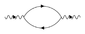
Figure 1: One-loop Feynman diagram describing the self-energy correction to graviton propagator due to matter field

The vertex associated with the interaction between graviton and scalar field in momentum space is expressed as

$$\mathcal{V}_{\mu\nu}(p,p+k,-k)=-\frac{\kappa}{2}[(p+k)_{\mu}k_{\nu}+(p+k)_{\nu}k_{\mu}-\eta_{\mu\nu}(p+k)^{\sigma}k_{\sigma}]\equiv\mathcal{P}_{\mu\nu}^{\ \ \rho\sigma}(p+k)_{\rho}k_{\sigma},$$ (5)

where

$$\mathcal{P}_{\mu\nu}^{\ \ \rho\sigma}=-\frac{\kappa}{2}\left(\delta_{\mu}^{\rho}\delta_{\nu}^{\sigma}+\delta_{\mu}^{\sigma}\delta_{\nu}^{\rho}-\eta_{\mu\nu}\eta^{\rho\sigma}\right).$$ (6)

From the free part of the scalar field, we may note that the scalar field propagator is $-i/p^{2}$ where $p^{\mu}$ is 4-momentum. To evaluate the self-energy corrections to gravitons, we evaluate the following integral corresponding to the above Feynman diagram:

$$\begin{split}\mathcal{I}&=-\int\frac{d^{D}k}{(2\pi)^{D}}\frac{1}{(p+k)^{2}k^{2}}\mathcal{P}_{\mu\nu}^{\ \ \rho\sigma}\mathcal{P}_{\alpha\beta}^{\ \ \gamma\delta}(p+k)_{\rho}k_{\sigma}(p+k)_{\gamma}k_{\delta}\\ &=-\mathcal{P}_{\mu\nu}^{\ \ \rho\sigma}\mathcal{P}_{\alpha\beta}^{\ \ \gamma\delta}\int\frac{d^{D}k}{(2\pi)^{D}}\int_{0}^{1}\frac{dx}{[(k+px)^{2}+p^{2}x(1-x)]^{2}}\\ &\times[p_{\rho}k_{\sigma}+k_{\rho}k_{\sigma}][p_{\gamma}k_{\delta}+k_{\gamma}k_{\delta}],\end{split}$$ (7)

where in the last line, we have used Feynman’s parametrization. Using the odd and even symmetries, the above integral reduces to:

$$\begin{split}\mathcal{I}&=-\mathcal{P}_{\mu\nu}^{\ \ \rho\sigma}\mathcal{P}_{\alpha\beta}^{\ \ \gamma\delta}\int\frac{d^{D}k}{(2\pi)^{D}}\int_{0}^{1}\frac{dx}{[(k+px)^{2}+p^{2}x(1-x)]^{2}}\\ &\times\Big{\{}p_{\rho}p_{\gamma}k_{\sigma}k_{\delta}(1-2x)^{2}+p_{\rho}p_{\sigma}p_{\gamma}p_{\delta}x^{2}(1-x)^{2}\\ &+p_{\rho}p_{\sigma}k_{\gamma}k_{\delta}x(x-1)+k_{\rho}k_{\sigma}p_{\gamma}p_{\delta}x(x-1)+k_{\rho}k_{\sigma}k_{\gamma}k_{\delta}\Big{\}}\\ &\equiv-\mathcal{P}_{\mu\nu}^{\ \ \rho\sigma}\mathcal{P}_{\alpha\beta}^{\ \ \gamma\delta}[I_{\rho\sigma\gamma\delta}^{(1)}+I_{\rho\sigma\gamma\delta}^{(2)}+I_{\rho\sigma\gamma\delta}^{(3)}+I_{\rho\sigma\gamma\delta}^{(4)}+I_{\rho\sigma\gamma\delta}^{(5)}].\end{split}$$ (8)

We can evaluate the above integrals for $D=4$. As shown in Appendix (C.1), we can explicitly evaluate up to $1/\epsilon$ order (where $\epsilon=4-D$).

Hence, in $D\rightarrow 4$ dimensions, the one-loop correction to the quantum effective action due to the scalar field is

$$S_{\rm corr}^{(2)}=-\frac{\alpha}{4\epsilon}\int d^{4}x\left[8\kappa^{2}h^{\alpha\beta}(\Box)^{2}h_{\alpha\beta}+4\kappa^{2}h(\Box)^{2}h\right]\,,$$ (9)

where

$$\alpha=\frac{1}{120(4\pi)^{2}}$$ (10)

We are now in a position to compare the above expression with the expression with the general quadratic gravity action:

$$S_{\rm quad}=\int d^{4}x\sqrt{-g}\left[aR_{\mu\nu\rho\sigma}R^{\mu\nu\rho\sigma}+bR_{\mu\nu}R^{\mu\nu}+cR^{2}\right]\,,$$ (11)

where $a,b$ and $c$ are coupling constants. Linearising the above action w.r.t the Minkowski background, as shown in Appendix (D) and comparing with Eq. (9), we obtain the following relations:

$$4a+b=-\frac{8\alpha}{\epsilon},\ c-a=-\frac{4\alpha}{\epsilon},$$ (12)

Redefining the coupling constants as:

$$a=-\frac{\alpha}{\epsilon}\bar{a},\ b=-\frac{\alpha}{\epsilon}\bar{b},\ c=-\frac{\alpha}{\epsilon}\bar{c},$$ (13)

we obtain the following relations

$$4\bar{a}+\bar{b}=8,\ \bar{c}-\bar{a}=4.$$ (14)

Since we have two equations and three unknowns, we have an infinite number of solutions for $\bar{a},\bar{b},\bar{c}$. Rewriting $\bar{b}$ and $\bar{c}$ in-terms of $\bar{a}$ we can write the quantum correction to the effective action (9) as follows

$$S_{corr}^{(2)} = -\frac{\alpha}{\epsilon}\bar{a}\int d^{4}x\sqrt{-g}\Big{[}R_{\mu\nu\rho\sigma}R^{\mu\nu\rho\sigma}-4R_{\mu\nu}R^{\mu\nu}+R^{2}\Big{]}$$ (15)

$$- \frac{\alpha}{\epsilon}\int d^{4}x\sqrt{-g}\Big{[}8R_{\mu\nu}R^{\mu\nu}+4R^{2}\Big{]}\,.$$

This is the first key result regarding which we want to discuss the following points: First, the term inside the first integral in the RHS of the above expression is the GB term and is proportional to $(D-4)$ [42]. Since the prefactor is proportional to $1/\epsilon=1/(4-D)$, $(D-4)$ factor that makes the GB term topological in 4-D cancels, leading to a dynamical 4-D GB term. As mentioned earlier, there have been many attempts in the literature to have a systematic procedure for making the 4-D GB term non-topological; our analysis shows that coupling the massless scalar field to gravity can naturally lead to such a non-topological term. Our analysis shows that the effect of matter at the one-loop level generates a term related to the non-topological GB gravity. To our knowledge, such an analysis has not been shown in the literature. Second, the term inside the second parenthesis acts as a counter-term, which must be added to the tree-level action to cancel this diverging term. Third, while the analysis is done for a massless scalar field, the results can be straightforwardly extended for self-interacting potential terms. Note that the subleading term $(\epsilon^{0})$ does not modify the GB term.

III Effect of interaction between Gravitons and Dirac fermions at 1-loop

The above result naturally leads to the following questions: How generic is the above result? What happens to the Fermions? In this section, we consider a massless Dirac field minimally coupled to gravity to address this. The action for such a field is:

$$S=\frac{1}{2\kappa^{2}}\int d^{4}x\ \sqrt{-g}R-\int d^{4}x\sqrt{-g}\bar{\psi}ie_{\ a}^{\mu}\gamma^{a}\mathcal{D}_{\mu}\psi,$$ (16)

where $\psi$ is a massless Dirac field, $e_{\ a}^{\mu}$ are tetrads satisfying the relation $g_{\mu\nu}e_{\ a}^{\mu}e_{\ b}^{\nu}=\eta_{ab}$, $\gamma^{a}$s are the Dirac gamma matrices satisfying the Clifford algebra $\{\gamma^{a},\gamma^{b}\}=-2\eta^{ab}$, and $\mathcal{D}_{\mu}=\partial_{\mu}+\Gamma_{\mu}$ is the spin-covariant derivative.

Like in the previous section, to keep things transparent, we consider the first-order perturbations ($h_{\mu\nu}$) about the Minkowski background: $g_{\mu\nu}=\eta_{\mu\nu}+\kappa h_{\mu\nu}$. The expansion of the Einstein-Hilbert action up to the second order in the metric perturbation is identical. Following the approach in the previous section, we may write the matter action as:

$$S_{M}[\psi]=-\int d^{4}x\bar{\psi}i\gamma^{\mu}\partial_{\mu}\psi+\kappa\int d^{4}xh_{\mu\nu}T^{\mu\nu},$$ (17)

where the energy-momentum tensor of massless Dirac field theory in Minkowski spacetime is given by

$$T^{\mu\nu}=\frac{i}{4}\bar{\psi}[\gamma^{\mu}\overrightarrow{\partial}^{\nu}+\gamma^{\nu}\overrightarrow{\partial}^{\mu}-\gamma^{\mu}\overleftarrow{\partial}^{\nu}-\gamma^{\nu}\overleftarrow{\partial}^{\mu}]\psi.$$ (18)

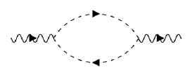
Figure 2: One-loop Feynman diagram describing the self-energy correction to graviton propagator due to matter field

Like earlier, as described by the Feynman diagram in Fig. 2, we now compute the self-energy correction to graviton due to matter one-loop. In this case, the vertex in momentum space associated with the graviton-fermion interaction is given by [ref]:

$$\begin{split}V^{\mu\nu}(p,q)&=-\frac{i\kappa}{8}[(p-q)^{\mu}\gamma^{\nu}+(p-q)^{\nu}\gamma^{\mu}-\eta^{\mu\nu}(\not{p}-\not{q})]\\ &\equiv-\frac{i\kappa}{8}\mathcal{P}_{\ \ \rho\sigma}^{\mu\nu}(p-q)^{\rho}\gamma^{\sigma},\end{split}$$ (19)

where

$$\mathcal{P}_{\ \ \rho\sigma}^{\mu\nu}=\delta_{\rho}^{\mu}\delta_{\sigma}^{\nu}+\delta_{\sigma}^{\mu}\delta_{\rho}^{\nu}-\eta^{\mu\nu}\eta_{\rho\sigma}.$$ (20)

To evaluate the self-energy corrections to gravitons, we evaluate the following integral corresponding to the above Feynman diagram (2):

$$\mathcal{J}^{\mu\nu\alpha\beta}=-\mathcal{P}_{\ \ \rho\sigma}^{\mu\nu}\mathcal{P}_{\ \ \gamma\delta}^{\alpha\beta}\frac{\kappa^{2}}{64}\int\frac{d^{D}k}{(2\pi)^{D}}\text{Tr}\Big{[}(p+2k)^{\rho}\gamma^{\sigma}\frac{1}{\not{p}+\not{k}}$$

$$\qquad\times(p+2k)^{\gamma}\gamma^{\delta}\frac{1}{\not{k}}\Big{]}$$

$$=-\mathcal{P}_{\ \ \rho\sigma}^{\mu\nu}\mathcal{P}_{\ \ \gamma\delta}^{\alpha\beta}\frac{\kappa^{2}}{16}\int\frac{d^{D}k}{(2\pi)^{D}}\frac{(p+2k)^{\rho}(p+2k)^{\gamma}}{k^{2}(p+k)^{2}}$$

$$\qquad(p+k)_{\alpha}k_{\beta}\times(\eta^{\sigma\alpha}\eta^{\delta\beta}-\eta^{\sigma\delta}\eta^{\alpha\beta}+\eta^{\sigma\beta}\eta^{\alpha\delta}).$$ (21)

As shown in Appendix (C.2), we can explicitly evaluate up to $1/\epsilon$ order leading to:

$$-ih_{\mu\nu}(-p)\mathcal{J}^{\mu\nu\alpha\beta}h_{\alpha\beta}(p)=\frac{\kappa^{2}\beta}{4\epsilon}p^{4}[h_{\mu\nu}(-p)h^{\mu\nu}(p)-2h(-p)h(p)]\,.$$ (22)

Thus, the correction to the quantum effective action is:

$$S_{\text{corr}}^{(2)}=\frac{\beta}{4\epsilon}\int d^{4}x\Big{[}\kappa^{2}h_{\mu\nu}(\Box)^{2}h^{\mu\nu}-2\kappa^{2}h(\Box)^{2}h\Big{]}\,,$$ (23)

where

$$\beta=\frac{1}{5(4\pi)^{2}}\,.$$

Like in the scalar field case, we can compare the above term with the quadratic gravity action (11). Expanding the action (11) to the second-order in the metric perturbations and comparing with the above correction action, we obtain the following relations

$$4a+b=\frac{\beta}{\epsilon},\ c-a=-\frac{2\beta}{\epsilon}\,.$$ (24)

Rewriting the coupling constants as

$$a=\frac{\beta}{\epsilon}\bar{a},\ b=\frac{\beta}{\epsilon}\bar{b},\ c=\frac{\beta}{\epsilon}\bar{c},$$ (25)

we obtain the following relations

$$4\bar{a}+\bar{b}=1,\ \bar{c}-\bar{a}=-2.$$ (26)

Now, we can write the quantum correction to the effective action as follows

$$S_{corr}^{(2)} = \frac{\beta}{\epsilon}\bar{a}\int d^{4}x\sqrt{-g}\Big{[}R_{\mu\nu\rho\sigma}R^{\mu\nu\rho\sigma}-4R_{\mu\nu}R^{\mu\nu}+R^{2}\Big{]}$$ (27)

$$+ \frac{\beta}{\epsilon}\int d^{4}x\sqrt{-g}\Big{[}R_{\mu\nu}R^{\mu\nu}-2R^{2}\Big{]},$$

This is the second key result regarding which we want to discuss the following points: First, like in the scalar field case, the term inside the first integral in the RHS of the above expression is the GB term and is proportional to $(D-4)$ [42]. Since the prefactor is proportional to $1/\epsilon=1/(4-D)$, $(D-4)$ factor that makes the GB term topological in 4-D cancels, leading to a dynamical 4-D GB term. Our analysis shows that the minimal coupling of the matter field with gravity naturally leads to a non-topological term. Second, the term inside the second parenthesis acts as a counter-term, which must be added to the tree-level action to cancel this diverging term. It is important to note that $R_{\mu\nu}R^{\mu\nu}$ counter-term for the scalar and Dirac fields have opposite signs. This is not unexpected since the one-loop computation of the Fermions involves trace operation with a negative sign due to the anti-commutation relation of the field variables. For this reason, the sign in front of $R_{\mu\nu}R^{\mu\nu}$ counter-term and the overall sign in front of the Gauss-Bonnet term is opposite compared to the scalar matter field.

IV Discussion

GR fails to be universally applicable in strong-field gravity because the higher-derivative corrections to the Einstein-Hilbert action become significant in this regime. Consequently, various observables, such as the photon sphere around a black hole and the cataclysmic events like binary black hole mergers, can undergo significant alterations. The simplest form of a higher-order modified gravity theory is the Einstein-Gauss-Bonnet gravity theory, which possesses a second-order equation of motion and is devoid of ghosts. However, this theory is primarily topological in four dimensions, as previously mentioned, and classically does not modify the equation of motion. Conversely, Glavan and Lin proposed a mathematical prescription to render the non-topological Gauss-Bonnet gravity theory in four dimensions [43].

Nevertheless, this prescription appears ad-hoc at first glance and lacks a solid mathematical motivation from the quantum field theory perspective [45]. In this study, we have provided a well-defined mathematical approach to derive the above prescription. To obtain such a prescription, we have utilized the technique of dimensional regularization, commonly employed in quantum field theory, to regulate divergences. Our analysis commenced with the linearized Einstein-Hilbert action coupled to massless matter field theories, specifically scalar and fermionic matter. We computed the self-energy correction to gravitons due to matter up to one-loop. After incorporating appropriate counterterms, we obtained the Einstein-Gauss-Bonnet gravity theory with a dimensional regularization parameter. This result unequivocally demonstrates that the simplest version of Lovelock gravity, namely the Einstein-Gauss-Bonnet gravity theory, can be rendered non-topological in 4-D when accounting for the quantum effects of matter on gravity.

The significance of our present work lies in its ability to introduce a novel perspective on the 4-D Einstein-Gauss-Bonnet gravity theory. First, in the context of early Universe cosmology, it was shown that Higgs field non-minimally coupled to the Gauss-Bonnet term can lead to inflation with an exit depending on the energy scale [78]. With the non-topological Einstein-Gauss-Bonnet gravity theory now available in four dimensions, it is worth exploring whether a qualitatively similar conclusion can be reached without the presence of the Higgs field. Second, the non-topological Gauss-Bonnet term is significant in investigating the formation and evaporation of primordial black holes in the early universe. This is because the Hawking temperature and Kretschmann scalar of an asymptotically flat space-time exhibit an inverse proportionality to the black hole mass. As a result, the Gauss-Bonnet term assumes a dominant role for primordial black holes, especially considering that their masses are anticipated to range between $10^{15}$ and $10^{26}$ grams [79, 80].

Third, our approach enables the examination of higher loop self-energy correction terms to ascertain whether higher-order Lovelock terms can be derived similarly [42]. Furthermore, it would be appealing to conduct a similar analysis while considering metric perturbations around a curved space-time in a covariant manner, especially for asymptotic non-flat space-times. Finally, it would be interesting if our work can be extended to the general effective field theory of gravity coupled to the Standard Model of particle physics [81]. This is currently under investigation.

V Acknowledgement

The authors thank S. Chakraborty and K. Lochan for discussions. SM is supported by SERB-Core Research Grant (Project RD/0122-SERB000-044).

Appendix A Linearised gravity

Although this is a standard calculation, for ease of verification, we compute the relevant quantities to obtain the linearised theory of gravity within the framework of Einstein’s general relativity in this appendix. In order to do that we consider the following decomposition of the metric

$$g_{\mu\nu}=\bar{g}_{\mu\nu}+\varepsilon h_{\mu\nu},$$ (28)

where $\bar{g}_{\mu\nu}$ is the metric describing the background geometry w.r.t which we linearised the theory of gravity, $h_{\mu\nu}$ is the metric perturbation and $\varepsilon$ carries the order of the metric perturbation. This leads to the following expression of the inverse metric

$$g^{\mu\nu}=\bar{g}^{\mu\nu}-\varepsilon h^{\mu\nu}+\varepsilon^{2}h^{\mu\rho}h_{\ \rho}^{\nu}+\mathcal{O}(\varepsilon^{3}),$$ (29)

where $\bar{g}^{\mu\nu}$ is the inverse metric of the background spacetime, and $h^{\mu\nu}$ is a rank-2 contravariant tensor defined by contracting the metric perturbation w.r.t the inverse metric $\bar{g}^{\mu\nu}$. Given the above set of relation, we are now able to compute the Christoffel symbol defined in the following manner

$$\Gamma_{\ \mu\nu}^{\rho}=\frac{1}{2}g^{\rho\lambda}(\partial_{\mu}g_{\lambda\nu}+\partial_{\nu}g_{\mu\lambda}-\partial_{\lambda}g_{\mu\nu}),$$ (30)

which reduces to the following form after using the relations (28) and (29)

$$\begin{split}\Gamma_{\ \mu\nu}^{\rho}&=\bar{\Gamma}_{\ \mu\nu}^{\rho}+\varepsilon\Big{[}\frac{1}{2}\bar{g}^{\rho\lambda}(\partial_{\mu}h_{\lambda\nu}+\partial_{\nu}h_{\mu\lambda}-\partial_{\lambda}h_{\mu\nu})\\ &-\bar{g}^{\rho\alpha}h_{\alpha\beta}\bar{\Gamma}_{\ \mu\nu}^{\beta}\Big{]}-\varepsilon^{2}\Big{[}\frac{1}{2}\bar{g}^{\beta\lambda}h_{\ \beta}^{\rho}(\partial_{\mu}h_{\lambda\nu}+\partial_{\nu}h_{\mu\lambda}-\partial_{\lambda}h_{\mu\nu})\\ &-\bar{g}^{\alpha\beta}h_{\ \beta}^{\rho}h_{\alpha\sigma}\bar{\Gamma}_{\ \mu\nu}^{\sigma}\Big{]},\end{split}$$ (31)

where

$$\bar{\Gamma}_{\ \mu\nu}^{\rho}=\frac{1}{2}\bar{g}^{\rho\lambda}(\partial_{\mu}\bar{g}_{\lambda\nu}+\partial_{\nu}\bar{g}_{\mu\lambda}-\partial_{\lambda}\bar{g}_{\mu\nu}).$$ (32)

After a change in the indices of the following form

$$\begin{split}\bar{g}^{\rho\alpha}h_{\alpha\beta}\bar{\Gamma}_{\ \mu\nu}^{\beta}&\rightarrow\bar{g}^{\rho\lambda}h_{\lambda\beta}\bar{\Gamma}_{\ \mu\nu}^{\beta}\\ \bar{g}^{\alpha\beta}h_{\ \beta}^{\rho}h_{\alpha\sigma}\bar{\Gamma}_{\ \mu\nu}^{\sigma}&\rightarrow\bar{g}^{\lambda\beta}h_{\ \beta}^{\rho}h_{\lambda\sigma}\bar{\Gamma}_{\ \mu\nu}^{\sigma},\end{split}$$ (33)

we obtain the following expression of Christoffel symbols

$$\begin{split}\Gamma_{\ \mu\nu}^{\rho}&=\bar{\Gamma}_{\ \mu\nu}^{\rho}+\frac{\varepsilon}{2}\bar{g}^{\rho\lambda}[\partial_{\mu}h_{\lambda\nu}+\partial_{\nu}h_{\mu\lambda}-\partial_{\lambda}h_{\mu\nu}-2h_{\lambda\beta}\bar{\Gamma}_{\ \mu\nu}^{\beta}]\\ &-\frac{\varepsilon^{2}}{2}\bar{g}^{\beta\lambda}h_{\ \beta}^{\rho}[\partial_{\mu}h_{\lambda\nu}+\partial_{\nu}h_{\mu\lambda}-\partial_{\lambda}h_{\mu\nu}-2h_{\lambda\sigma}\bar{\Gamma}_{\ \mu\nu}^{\sigma}].\end{split}$$ (34)

Now adding and subtracting the following terms at different order

$$\begin{split}\mathcal{O}(\varepsilon):&h_{\mu\beta}\bar{\Gamma}_{\ \nu\lambda}^{\beta}+h_{\nu\beta}\bar{\Gamma}_{\ \mu\lambda}^{\beta}\\ \mathcal{O}(\varepsilon^{2}):&h_{\mu\sigma}\bar{\Gamma}_{\ \nu\lambda}^{\sigma}+h_{\nu\sigma}\bar{\Gamma}_{\ \mu\lambda}^{\sigma},\end{split}$$ (35)

and then regrouping the terms gives

$$\begin{split}\Gamma_{\ \mu\nu}^{\rho}&=\bar{\Gamma}_{\ \mu\nu}^{\rho}+\frac{\varepsilon}{2}\bar{g}^{\rho\lambda}(\bar{\nabla}_{\mu}h_{\lambda\nu}+\bar{\nabla}_{\nu}h_{\mu\lambda}-\bar{\nabla}_{\lambda}h_{\mu\nu})\\ &-\frac{\varepsilon^{2}}{2}h_{\ \beta}^{\rho}\bar{g}^{\beta\lambda}(\bar{\nabla}_{\mu}h_{\lambda\nu}+\bar{\nabla}_{\nu}h_{\mu\lambda}-\bar{\nabla}_{\lambda}h_{\mu\nu}),\end{split}$$ (36)

where we recognize the following

$$\bar{\nabla}_{\lambda}h_{\mu\nu}=\partial_{\lambda}h_{\mu\nu}-h_{\nu\sigma}\bar{\Gamma}_{\ \mu\lambda}^{\sigma}-h_{\mu\sigma}\bar{\Gamma}_{\ \nu\lambda}^{\sigma}.$$ (37)

Therefore, defining the linearised Christoffel symbol as

$$(\Gamma_{\ \mu\nu}^{\rho})_{L}=\frac{1}{2}\bar{g}^{\rho\lambda}(\bar{\nabla}_{\mu}h_{\lambda\nu}+\bar{\nabla}_{\nu}h_{\mu\lambda}-\bar{\nabla}_{\lambda}h_{\mu\nu}),$$ (38)

we may now write

$$\Gamma_{\ \mu\nu}^{\rho}=\bar{\Gamma}_{\ \mu\nu}^{\rho}+\varepsilon(\Gamma_{\ \mu\nu}^{\rho})_{L}-\varepsilon^{2}h_{\ \beta}^{\rho}(\Gamma_{\ \mu\nu}^{\beta})_{L}.$$ (39)

The Riemann curvature tensor is defined as

$$R_{\ \nu\rho\sigma}^{\mu}=\partial_{\rho}\Gamma_{\ \sigma\nu}^{\mu}+\Gamma_{\ \rho\lambda}^{\mu}\Gamma_{\ \sigma\nu}^{\lambda}-\partial_{\sigma}\Gamma_{\ \rho\nu}^{\mu}-\Gamma_{\ \sigma\lambda}^{\mu}\Gamma_{\ \rho\nu}^{\lambda}.$$ (40)

We start by defining the following quantity

$$\delta\Gamma_{\ \mu\nu}^{\rho}\equiv\Gamma_{\ \mu\nu}^{\rho}-\bar{\Gamma}_{\ \mu\nu}^{\rho}=\varepsilon(\Gamma_{\ \mu\nu}^{\rho})_{L}-\varepsilon^{2}h_{\ \beta}^{\rho}(\Gamma_{\ \mu\nu}^{\beta})_{L},$$ (41)

in terms of which we may express the Riemann curvature tensor as

$$\begin{split}R_{\ \nu\rho\sigma}^{\mu}&=\bar{R}_{\ \nu\rho\sigma}^{\mu}+(\partial_{\rho}\delta\Gamma_{\ \sigma\nu}^{\mu}+\bar{\Gamma}_{\ \rho\lambda}^{\mu}\delta\Gamma_{\ \sigma\nu}^{\lambda}-\bar{\Gamma}_{\ \rho\nu}^{\lambda}\delta\Gamma_{\ \sigma\lambda}^{\mu})\\ &-(\partial_{\sigma}\delta\Gamma_{\ \rho\nu}^{\mu}+\bar{\Gamma}_{\ \sigma\lambda}^{\mu}\delta\Gamma_{\ \rho\nu}^{\lambda}-\bar{\Gamma}_{\ \sigma\nu}^{\lambda}\delta\Gamma_{\ \rho\lambda}^{\mu})\\ &+\delta\Gamma_{\ \rho\lambda}^{\mu}\delta\Gamma_{\ \sigma\nu}^{\lambda}-\delta\Gamma_{\ \sigma\lambda}^{\mu}\delta\Gamma_{\ \rho\nu}^{\lambda},\end{split}$$ (42)

where

$$\bar{R}_{\ \nu\rho\sigma}^{\mu}=\partial_{\rho}\bar{\Gamma}_{\ \sigma\nu}^{\mu}+\bar{\Gamma}_{\ \rho\lambda}^{\mu}\bar{\Gamma}_{\ \sigma\nu}^{\lambda}-\partial_{\sigma}\bar{\Gamma}_{\ \rho\nu}^{\mu}-\bar{\Gamma}_{\ \sigma\lambda}^{\mu}\bar{\Gamma}_{\ \rho\nu}^{\lambda}.$$ (43)

Now adding and subtracting the term $\bar{\Gamma}_{\ \rho\sigma}^{\lambda}\delta\Gamma_{\ \lambda\nu}^{\mu}$ from the equation (42), we obtain the following relation

$$R_{\ \nu\rho\sigma}^{\mu}=\bar{R}_{\ \nu\rho\sigma}^{\mu}+\bar{\nabla}_{\rho}\delta\Gamma_{\ \sigma\nu}^{\mu}-\bar{\nabla}_{\sigma}\delta\Gamma_{\ \rho\nu}^{\mu}+\delta\Gamma_{\ \rho\lambda}^{\mu}\delta\Gamma_{\ \sigma\nu}^{\lambda}-\delta\Gamma_{\ \sigma\lambda}^{\mu}\delta\Gamma_{\ \rho\nu}^{\lambda}.$$ (44)

Now using the relation (41), we now express the above relation as follows

$$\begin{split}R_{\ \nu\rho\sigma}^{\mu}&=\bar{R}_{\ \nu\rho\sigma}^{\mu}+\varepsilon[\bar{\nabla}_{\rho}(\Gamma_{\ \sigma\nu}^{\mu})_{L}-\bar{\nabla}_{\sigma}(\bar{\Gamma}_{\ \rho\nu}^{\mu})_{L}]\\ &-\varepsilon^{2}\{\bar{\nabla}_{\rho}[h_{\ \beta}^{\mu}(\Gamma_{\ \sigma\nu}^{\beta})_{L}]-\bar{\nabla}_{\sigma}[h_{\ \beta}^{\mu}(\Gamma_{\ \rho\nu}^{\beta})_{L}]\\ &-(\Gamma_{\ \rho\lambda}^{\mu})_{L}(\Gamma_{\ \sigma\nu}^{\lambda})_{L}+(\Gamma_{\ \sigma\lambda}^{\mu})_{L}(\Gamma_{\ \rho\nu}^{\lambda})_{L}\}+\mathcal{O}(\varepsilon^{3}).\end{split}$$ (45)

The above expression can further be reduced in the following form

$$\begin{split}R_{\ \nu\rho\sigma}^{\mu}&=\bar{R}_{\ \nu\rho\sigma}^{\mu}+\varepsilon\{\bar{\nabla}_{\rho}(\Gamma_{\ \sigma\nu}^{\mu})_{L}-\bar{\nabla}_{\sigma}(\Gamma_{\ \rho\nu}^{\mu})_{L}\}\\ &-\varepsilon^{2}\{h_{\ \beta}^{\mu}[\bar{\nabla}_{\rho}(\Gamma_{\ \sigma\nu}^{\beta})_{L}-\bar{\nabla}_{\sigma}(\Gamma_{\ \rho\nu}^{\beta})_{L}]\\ &+(\Gamma_{\ \sigma\nu}^{\beta})_{L}\bar{\nabla}_{\rho}h_{\ \beta}^{\mu}-(\Gamma_{\ \rho\nu}^{\beta})_{L}\bar{\nabla}_{\sigma}h_{\ \beta}^{\mu}\\ &-(\Gamma_{\ \rho\beta}^{\mu})_{L}(\Gamma_{\ \sigma\nu}^{\beta})_{L}+(\Gamma_{\ \sigma\beta}^{\mu})_{L}(\Gamma_{\ \rho\nu}^{\beta})_{L}\}.\end{split}$$ (46)

Defining the following quantity

$$(R_{\ \nu\rho\sigma}^{\mu})_{L}=\bar{\nabla}_{\rho}(\Gamma_{\ \sigma\nu}^{\mu})_{L}-\bar{\nabla}_{\sigma}(\Gamma_{\ \rho\nu}^{\mu})_{L},$$ (47)

we further reduce the expression of Riemann curvature tensor as

$$\begin{split}R_{\ \nu\rho\sigma}^{\mu}&=\bar{R}_{\ \nu\rho\sigma}^{\mu}+\varepsilon(R_{\ \nu\rho\sigma}^{\mu})_{L}-\varepsilon^{2}\{h_{\ \beta}^{\mu}(R_{\ \nu\rho\sigma}^{\beta})_{L}\\ &+(\Gamma_{\ \sigma\nu}^{\beta})_{L}[\bar{\nabla}_{\rho}h_{\ \beta}^{\mu}-(\Gamma_{\ \rho\beta}^{\mu})_{L}]\\ &-(\Gamma_{\ \rho\nu}^{\beta})_{L}[\bar{\nabla}_{\sigma}h_{\ \beta}^{\mu}-(\Gamma_{\ \sigma\beta}^{\mu})_{L}]\}.\end{split}$$ (48)

The term $*\equiv(\Gamma_{\ \sigma\nu}^{\beta})_{L}[\bar{\nabla}_{\rho}h_{\ \beta}^{\mu}-(\Gamma_{\ \rho\beta}^{\mu})_{L}]$ can be expressed as

$$\begin{split}*&=(\Gamma_{\ \sigma\nu}^{\beta})_{L}\Big{[}\bar{\nabla}_{\rho}(\bar{g}^{\mu\alpha}h_{\alpha\beta})-\frac{1}{2}\bar{g}^{\mu\alpha}(\bar{\nabla}_{\rho}h_{\alpha\beta}+\bar{\nabla}_{\beta}h_{\rho\alpha}-\bar{\nabla}_{\alpha}h_{\rho\beta})\Big{]}\\ &=(\Gamma_{\ \sigma\nu}^{\beta})_{L}\Big{[}\frac{1}{2}\bar{g}^{\mu\alpha}(\bar{\nabla}_{\rho}h_{\alpha\beta}+\bar{\nabla}_{\alpha}h_{\rho\beta}-\bar{\nabla}_{\beta}h_{\rho\alpha})\Big{]}\\ &=(\Gamma_{\ \sigma\nu}^{\beta})_{L}\Big{[}\frac{1}{2}\bar{g}^{\mu\alpha}\delta_{\beta}^{\ \lambda}(\bar{\nabla}_{\rho}h_{\alpha\lambda}+\bar{\nabla}_{\alpha}h_{\rho\lambda}-\bar{\nabla}_{\lambda}h_{\rho\alpha})\Big{]}\\ &=(\Gamma_{\ \sigma\nu}^{\beta})_{L}\Big{[}\frac{1}{2}\bar{g}^{\mu\alpha}\bar{g}_{\beta\gamma}\bar{g}^{\gamma\lambda}(\bar{\nabla}_{\rho}h_{\alpha\lambda}+\bar{\nabla}_{\alpha}h_{\rho\lambda}-\bar{\nabla}_{\lambda}h_{\rho\alpha})\Big{]}\\ &=\bar{g}^{\mu\alpha}\bar{g}_{\beta\gamma}(\Gamma_{\ \sigma\nu}^{\beta})_{L}(\Gamma_{\ \rho\alpha}^{\gamma})_{L}.\end{split}$$ (49)

In the similar manner, we may express the following

$$(\Gamma_{\ \rho\nu}^{\beta})_{L}[\bar{\nabla}_{\sigma}h_{\ \beta}^{\mu}-(\Gamma_{\ \sigma\beta}^{\mu})_{L}]=\bar{g}^{\mu\alpha}\bar{g}_{\beta\gamma}(\Gamma_{\ \rho\nu}^{\beta})_{L}(\Gamma_{\ \sigma\alpha}^{\gamma})_{L}.$$ (50)

Using the above results, the final form of the Riemann tensor perturbed up to second order in metric perturbation is given as

$$\begin{split}R_{\ \nu\rho\sigma}^{\mu}&=\bar{R}_{\ \nu\rho\sigma}^{\mu}+\varepsilon(R_{\ \nu\rho\sigma}^{\mu})_{L}-\varepsilon^{2}\{h_{\ \beta}^{\mu}(R_{\ \nu\rho\sigma}^{\beta})_{L}\\ &+\bar{g}^{\mu\alpha}\bar{g}_{\beta\gamma}[(\Gamma_{\ \sigma\nu}^{\beta})_{L}(\Gamma_{\ \rho\alpha}^{\gamma})_{L}-(\Gamma_{\ \rho\nu}^{\beta})_{L}(\Gamma_{\ \sigma\alpha}^{\gamma})_{L}]\}.\end{split}$$ (51)

As a result, the Ricci tensor can be expressed as

$$\begin{split}R_{\nu\sigma}&=\bar{R}_{\nu\sigma}+\varepsilon(R_{\nu\sigma})_{L}-\varepsilon^{2}\{h_{\ \beta}^{\mu}(R_{\ \nu\mu\sigma}^{\beta})_{L}\\ &+\bar{g}^{\mu\alpha}\bar{g}_{\beta\gamma}[(\Gamma_{\ \sigma\nu}^{\beta})_{L}(\Gamma_{\ \mu\alpha}^{\gamma})_{L}-(\Gamma_{\ \mu\nu}^{\beta})_{L}(\Gamma_{\ \sigma\alpha}^{\gamma})_{L}]\}.\end{split}$$ (52)

From the definition of linearised Riemann tensor, we have the following expression

$$\begin{split}(R_{\ \nu\rho\sigma}^{\mu})_{L}&=\frac{1}{2}[\bar{\nabla}_{\rho}\bar{\nabla}_{\sigma}h_{\ \nu}^{\mu}+\bar{\nabla}_{\rho}\bar{\nabla}_{\nu}h_{\ \sigma}^{\mu}-\bar{\nabla}_{\rho}\bar{\nabla}^{\mu}h_{\sigma\nu}\\ &-\bar{\nabla}_{\sigma}\bar{\nabla}_{\rho}h_{\ \nu}^{\mu}-\bar{\nabla}_{\sigma}\bar{\nabla}_{\nu}h_{\ \rho}^{\mu}+\bar{\nabla}_{\sigma}\bar{\nabla}^{\mu}h_{\rho\nu}],\end{split}$$ (53)

which leads to the following expression of $(R_{\nu\sigma})_{L}$

$$\begin{split}(R_{\nu\sigma})_{L}&=(R_{\ \nu\mu\sigma}^{\mu})_{L}\\ &=\frac{1}{2}(\bar{\nabla}_{\mu}\bar{\nabla}_{\sigma}h_{\ \nu}^{\mu}+\bar{\nabla}_{\mu}\bar{\nabla}_{\nu}h_{\ \sigma}^{\mu}-\bar{\Box}h_{\sigma\nu}-\bar{\nabla}_{\sigma}\bar{\nabla}_{\nu}h).\end{split}$$ (54)

Therefore, the Ricci scalar can now be expressed as

$$\begin{split}R&=(\bar{g}^{\nu\sigma}-\varepsilon h^{\nu\sigma}+\varepsilon^{2}h^{\nu\lambda}h_{\ \lambda}^{\sigma})[\bar{R}_{\nu\sigma}+\varepsilon(R_{\nu\sigma})_{L}\\ &-\varepsilon^{2}\{h_{\ \beta}^{\mu}(R_{\ \nu\mu\sigma}^{\beta})_{L}+\bar{g}^{\mu\alpha}\bar{g}_{\beta\gamma}[(\Gamma_{\ \sigma\nu}^{\beta})_{L}(\Gamma_{\ \mu\alpha}^{\gamma})_{L}\\ &-(\Gamma_{\ \mu\nu}^{\beta})_{L}(\Gamma_{\ \sigma\alpha}^{\gamma})_{L}]\}]\\ &=\bar{g}^{\nu\sigma}\bar{R}_{\nu\sigma}+\varepsilon[\bar{g}^{\nu\sigma}(R_{\nu\sigma})_{L}-h^{\nu\sigma}\bar{R}_{\nu\sigma}]\\ &-\varepsilon^{2}[\bar{g}^{\nu\sigma}\{h_{\ \beta}^{\mu}(R_{\ \nu\mu\sigma}^{\beta})_{L}+\bar{g}^{\mu\alpha}\bar{g}_{\beta\gamma}[(\Gamma_{\ \sigma\nu}^{\beta})_{L}(\Gamma_{\ \mu\alpha}^{\gamma})_{L}\\ &-(\Gamma_{\ \mu\nu}^{\beta})_{L}(\Gamma_{\ \sigma\alpha}^{\gamma})_{L}]\}+h^{\nu\sigma}(R_{\nu\sigma})_{L}-h^{\nu\lambda}h_{\ \lambda}^{\sigma}\bar{R}_{\nu\sigma}]+\mathcal{O}(\varepsilon^{3}).\end{split}$$ (55)

Using the following definitions

$$\bar{R}=\bar{g}^{\nu\sigma}\bar{R}_{\nu\sigma},\ R_{L}=\bar{g}^{\nu\sigma}(R_{\nu\sigma})_{L}-h^{\nu\sigma}\bar{R}_{\nu\sigma},$$ (56)

and neglecting the higher order contributions, we obtain the following form of Ricci scalar

$$\begin{split}R&=\bar{R}+\varepsilon R_{L}-\varepsilon^{2}\{\bar{g}^{\nu\sigma}h_{\ \beta}^{\mu}(R_{\ \nu\mu\sigma}^{\beta})_{L}+h^{\nu\sigma}(R_{\nu\sigma})_{L}\\ &-h^{\nu\lambda}h_{\ \lambda}^{\sigma}\bar{R}_{\nu\sigma}+\bar{g}^{\nu\sigma}\bar{g}^{\mu\alpha}\bar{g}_{\beta\gamma}[(\Gamma_{\ \sigma\nu}^{\beta})_{L}(\Gamma_{\ \mu\alpha}^{\gamma})_{L}\\ &-(\Gamma_{\ \mu\nu}^{\beta})_{L}(\Gamma_{\ \sigma\alpha}^{\gamma})_{L}]\}.\end{split}$$ (57)

Appendix B Linearised gravity in Einstein-Hilbert action

In this appendix, we describe the linearised theory of Einstein’s general relativity by expressing the Einstein-Hilbert action in terms of metric perturbation w.r.t the Minkowski flat spacetime. The Einstein-Hilbert action is expressed as

$$S_{EH}=\frac{1}{2\kappa^{2}}\int d^{4}x\sqrt{-g}R,$$ (58)

where $g$ is the determinant of the metric of the spacetime and $\kappa^{2}=8\pi G$ in natural units. In order to make the above-mentioned expansion, we consider the following decomposition of the metric tensor

$$g_{\mu\nu}=\eta_{\mu\nu}+\kappa h_{\mu\nu},$$ (59)

which leads to the following inverse metric

$$g^{\mu\nu}=\eta^{\mu\nu}-\kappa h^{\mu\nu}.$$ (60)

Moreover, we also obtain the following relation

$$\sqrt{-g}\approx 1+\frac{\kappa}{2}h,$$ (61)

where $h=\eta^{\mu\nu}h_{\mu\nu}$. Hence, the expression of the Christoffel symbols become

$$\Gamma_{\ \mu\nu}^{\rho}=\frac{\kappa}{2}(\eta^{\rho\gamma}-\kappa h^{\rho\gamma})(\partial_{\nu}h_{\mu\gamma}+\partial_{\mu}h_{\nu\gamma}-\partial_{\gamma}h_{\mu\nu}).$$ (62)

As a result, up to first order, the expression of Christoffel symbols reduce to the following form

$$\Gamma_{\ \ \ \mu\nu}^{(1)\rho}=\frac{\kappa}{2}(\partial_{\nu}h_{\mu}^{\ \rho}+\partial_{\mu}h_{\nu}^{\ \rho}-\partial^{\rho}h_{\mu\nu}),$$ (63)

which leads to the following two relations

$$\begin{split}\partial_{\rho}\Gamma_{\ \ \ \mu\nu}^{(1)\rho}&=\frac{\kappa}{2}(\partial_{\rho}\partial_{\nu}h_{\mu}^{\ \rho}+\partial_{\rho}\partial_{\mu}h_{\nu}^{\ \rho}-\partial_{\rho}\partial^{\rho}h_{\mu\nu})\\ \partial_{\nu}\Gamma_{\ \ \ \mu\rho}^{(1)\rho}&=\frac{\kappa}{2}(\partial_{\nu}\partial_{\rho}h_{\ \mu}^{\rho}+\partial_{\nu}\partial_{\mu}h_{\ \rho}^{\rho}-\partial_{\nu}\partial^{\rho}h_{\mu\rho}).\end{split}$$ (64)

As a result, up to first order, the Ricci tensor can be expressed as

$$\begin{split}R_{\mu\nu}^{(1)}&=\partial_{\rho}\Gamma_{\ \ \ \mu\nu}^{(1)\rho}-\partial_{\nu}\Gamma_{\ \ \ \mu\rho}^{(1)\rho}\\ &=\frac{\kappa}{2}(\partial_{\rho}\partial_{\mu}h_{\nu}^{\ \rho}+\partial_{\nu}\partial^{\rho}h_{\mu\rho}-\partial_{\nu}\partial_{\mu}h-\Box h_{\mu\nu}),\end{split}$$ (65)

where $\Box=\partial_{\mu}\partial^{\mu}$. In order to obtain the second-order term for the Ricci tensor, we now use the following form of the second-order Christoffel symbols

$$\Gamma_{\ \ \ \mu\nu}^{(2)\rho}=-\frac{\kappa^{2}}{2}h^{\rho\gamma}(\partial_{\nu}h_{\mu\gamma}+\partial_{\mu}h_{\nu\gamma}-\partial_{\gamma}h_{\mu\nu}).$$ (66)

Using the above expression, we obtain the following results

$$\begin{split}\partial_{\rho}\Gamma_{\ \ \ \mu\nu}^{(2)\rho}&=-\frac{\kappa^{2}}{2}[\partial_{\rho}h^{\rho\gamma}(\partial_{\nu}h_{\mu\gamma}+\partial_{\mu}h_{\nu\gamma}-\partial_{\gamma}h_{\mu\nu})\\ &+h^{\rho\gamma}\partial_{\rho}(\partial_{\nu}h_{\mu\gamma}+\partial_{\mu}h_{\nu\gamma}-\partial_{\gamma}h_{\mu\nu})]\\ \partial_{\nu}\Gamma_{\ \ \ \mu\rho}^{(2)\rho}&=-\frac{\kappa^{2}}{2}[\partial_{\nu}h^{\rho\gamma}\partial_{\mu}h_{\rho\gamma}+h^{\rho\gamma}\partial_{\nu}\partial_{\mu}h_{\rho\gamma}],\end{split}$$ (67)

which eventually leads to the following result after some algebra

$$\begin{split}\partial_{\rho}\Gamma_{\ \ \ \mu\nu}^{(2)\rho}-\partial_{\nu}\Gamma_{\ \ \ \mu\rho}^{(2)\rho}&=-\frac{\kappa^{2}}{2}[\partial_{\rho}h^{\rho\gamma}(\partial_{\nu}h_{\mu\gamma}+\partial_{\mu}h_{\nu\gamma}-\partial_{\gamma}h_{\mu\nu})\\ &+h^{\rho\gamma}(\partial_{\rho}\partial_{\nu}h_{\mu\gamma}+\partial_{\rho}\partial_{\mu}h_{\nu\gamma}-\partial_{\rho}\partial_{\gamma}h_{\mu\nu}\\ &-\partial_{\nu}\partial_{\mu}h_{\rho\gamma})-\partial_{\nu}h^{\rho\gamma}\partial_{\mu}h_{\rho\gamma}].\end{split}$$ (68)

Moreover, we also have the following relations

$$\begin{split}\Gamma_{\ \ \ \gamma\rho}^{(1)\rho}\Gamma_{\ \ \ \mu\nu}^{(1)\gamma}&=\frac{\kappa^{2}}{4}[\partial_{\gamma}h(\partial_{\mu}h_{\nu}^{\ \gamma}+\partial_{\nu}h_{\mu}^{\ \gamma}-\partial^{\gamma}h_{\mu\nu})]\\ \Gamma_{\ \ \ \gamma\nu}^{(1)\rho}\Gamma_{\ \ \ \mu\rho}^{(1)\gamma}&=\frac{\kappa^{2}}{2}\Big{[}\partial_{\gamma}h_{\nu}^{\ \rho}(\partial_{\rho}h_{\mu}^{\ \gamma}-\partial^{\gamma}h_{\rho\mu})+\frac{1}{2}\partial_{\nu}h_{\gamma}^{\ \rho}\partial_{\mu}h_{\rho}^{\ \gamma}\Big{]}.\end{split}$$ (69)

Combining all these pieces gives us the total Ricci tensor in the second-order:

$$\begin{split}R_{\mu\nu}^{(2)}&=-\frac{\kappa^{2}}{2}\Big{[}\partial_{\rho}h^{\rho\gamma}(\partial_{\nu}h_{\mu\gamma}+\partial_{\mu}h_{\nu\gamma}-\partial_{\gamma}h_{\mu\nu})\\ &+h^{\rho\gamma}(\partial_{\rho}\partial_{\nu}h_{\mu\gamma}+\partial_{\rho}\partial_{\mu}h_{\nu\gamma}-\partial_{\rho}\partial_{\gamma}h_{\mu\nu}-\partial_{\nu}\partial_{\mu}h_{\rho\gamma})\\ &-\frac{1}{2}\partial_{\nu}h^{\rho\gamma}\partial_{\mu}h_{\rho\gamma}-\frac{1}{2}\partial_{\gamma}h(\partial_{\mu}h_{\nu}^{\ \gamma}+\partial_{\nu}h_{\mu}^{\ \gamma}-\partial^{\gamma}h_{\mu\nu})\\ &+\partial_{\gamma}h_{\nu}^{\ \rho}(\partial_{\rho}h_{\mu}^{\ \gamma}-\partial^{\gamma}h_{\rho\mu})\Big{]}.\end{split}$$ (70)

As a result, the Einstein-Hilbert action reduces to the following form up to quadratic order

$$\begin{split}S_{EH}^{(1)}+S_{EH}^{(2)}&=\frac{1}{2\kappa^{2}}\int d^{4}x\left(1+\frac{\kappa}{2}h\right)(\eta^{\mu\nu}-\kappa h^{\mu\nu})(R_{\mu\nu}^{(1)}+R_{\mu\nu}^{(2)})\\ &=\frac{1}{2\kappa^{2}}\int d^{4}x\Big{[}\eta^{\mu\nu}R_{\mu\nu}^{(1)}-\kappa h^{\mu\nu}R_{\mu\nu}^{(1)}+\frac{\kappa}{2}h\eta^{\mu\nu}R_{\mu\nu}^{(1)}\\ &+\eta^{\mu\nu}R_{\mu\nu}^{(2)}\Big{]},\end{split}$$ (71)

where

$$\begin{split}\eta^{\mu\nu}R_{\mu\nu}^{(1)}&=\kappa(\partial_{\rho}\partial_{\mu}h^{\rho\mu}-\Box h)\\ -\kappa h^{\mu\nu}R_{\mu\nu}^{(1)}&=-\frac{\kappa^{2}}{2}h^{\mu\nu}(\partial_{\rho}\partial_{\mu}h_{\nu}^{\ \rho}+\partial_{\nu}\partial^{\rho}h_{\mu\rho}-\partial_{\nu}\partial_{\mu}h-\Box h_{\mu\nu})\\ \frac{\kappa}{2}h\eta^{\mu\nu}R_{\mu\nu}^{(1)}&=\frac{\kappa^{2}}{2}(h\partial_{\rho}\partial_{\mu}h^{\rho\mu}-h\Box h)\\ \eta^{\mu\nu}R_{\mu\nu}^{(2)}&=-\frac{\kappa^{2}}{2}h\partial^{\gamma}\partial^{\mu}h_{\mu\gamma}+\frac{\kappa^{2}}{4}h\Box h+\frac{\kappa^{2}}{2}h^{\rho\gamma}\partial_{\rho}\partial^{\mu}h_{\mu\gamma}\\ &-\frac{\kappa^{2}}{4}h^{\rho\gamma}\Box h_{\rho\gamma}.\end{split}$$ (72)

Collecting all these contributions, neglecting boundary terms and scaling by a constant, the Einstein-Hilbert action up to second-order reduces to the following form

$$\begin{split}S_{EH}&=\int d^{D}x\Big{[}-\frac{1}{2}\partial_{\lambda}h_{\mu\nu}\partial^{\lambda}h^{\mu\nu}+\partial_{\mu}h_{\nu\lambda}\partial^{\nu}h^{\mu\lambda}-\partial_{\mu}h^{\mu\nu}\partial_{\nu}h\\ &+\frac{1}{2}\partial_{\lambda}h\partial^{\lambda}h\Big{]}.\end{split}$$ (73)

We may note that the above action is invariant under the following gauge transformation

$$h_{\mu\nu}\rightarrow h_{\mu\nu}+\partial_{\mu}\xi_{\nu}+\partial_{\nu}\xi_{\mu}.$$ (74)

The above action can also be expressed as

$$\begin{split}S_{EH}&=\int d^{D}x\frac{1}{2}h_{\mu\nu}\mathcal{E}^{\mu\nu,\alpha\beta}h_{\alpha\beta}\\ \mathcal{E}_{\ \ \ \alpha\beta}^{\mu\nu,}&=\left(\delta_{\alpha}^{(\mu}\delta_{\beta}^{\nu)}-\eta^{\mu\nu}\eta_{\alpha\beta}\right)\Box-2\partial^{(\mu}\partial_{(\alpha}\delta_{\beta)}^{\nu)}+\partial^{\mu}\partial^{\nu}\eta_{\alpha\beta}\\ &+\partial_{\alpha}\partial_{\beta}\eta^{\mu\nu}.\end{split}$$ (75)

We first note the action of the kinetic operator $\mathcal{E}^{\mu\nu,\alpha\beta}$ on a general symmetric tensor $\mathcal{Z}_{\alpha\beta}$

$$\begin{split}\mathcal{E}^{\mu\nu,\alpha\beta}\mathcal{Z}_{\alpha\beta}&=\Box\mathcal{Z}^{\mu\nu}-\eta^{\mu\nu}\Box\mathcal{Z}-2\partial^{(\mu}\partial_{\alpha}\mathcal{Z}^{\nu)\alpha}\\ &+\partial^{\mu}\partial^{\nu}\mathcal{Z}+\eta^{\mu\nu}\partial_{\alpha}\partial_{\beta}\mathcal{Z}^{\alpha\beta},\end{split}$$ (76)

which is a transverse tensor since

$$\partial_{\mu}(\mathcal{E}^{\mu\nu,\alpha\beta}\mathcal{Z}_{\alpha\beta})=0,$$ (77)

which can be checked quite easily. Furthermore, the kinetic operator would annihilate any pure gauge

$$\begin{split}\mathcal{E}^{\mu\nu,\alpha\beta}&(\partial_{\alpha}\xi_{\beta}+\partial_{\beta}\xi_{\alpha})=\Box(\partial^{\mu}\xi^{\nu}+\partial^{\nu}\xi^{\mu})-2\eta^{\mu\nu}\Box\partial_{\alpha}\xi^{\alpha}\\ &-\partial^{\mu}\partial_{\alpha}(\partial^{\nu}\xi^{\alpha}+\partial^{\alpha}\xi^{\nu})-\partial^{\nu}\partial_{\alpha}(\partial^{\mu}\xi^{\alpha}+\partial^{\alpha}\xi^{\mu})\\ &+2\partial^{\mu}\partial^{\nu}\partial_{\alpha}\xi^{\alpha}+\eta^{\mu\nu}\partial_{\alpha}\partial_{\beta}(\partial^{\alpha}\xi^{\beta}+\partial^{\beta}\xi^{\alpha})=0.\end{split}$$ (78)

As a result, the determinant of the kinetic operator vanishes which means it cannot be invertible. Therefore, in order to find the propagator in this theory, we must fix the gauge freedom in this theory. Here we choose the Lorenz gauge which is given by the following relation

$$\partial^{\mu}h_{\mu\nu}-\frac{1}{2}\partial_{\nu}h=0.$$ (79)

Therefore, given a metric perturbation, one can always do a gauge transformation

$$\delta h_{\mu\nu}=\partial_{\mu}\xi_{\nu}+\partial_{\nu}\xi_{\mu},$$ (80)

such that

$$\Box\xi_{\mu}=-\left(\partial^{\nu}h_{\mu\nu}-\frac{1}{2}\partial_{\mu}h\right),$$ (81)

which makes sure the gauge fixing condition is satisfied. However, this fixes the gauge up to gauge transformation $\xi_{\mu}$ satisfy the harmonicity condition $\Box\xi_{\mu}=0$. Besides that with this gauge choice, the equation of motion reduces to the following form

$$\Box h_{\mu\nu}-\frac{1}{2}\eta_{\mu\nu}\Box h=0,$$ (82)

and these are the gauge-fixed equations of motion. In order to obtain these equations of motion, we have to add a gauge fixing Lagrangian density which is of the following form

$$\mathcal{L}_{GF}=-\left(\partial^{\nu}h_{\mu\nu}-\frac{1}{2}\partial_{\mu}h\right)^{2}.$$ (83)

By doing that we obtain a neg Lagrangian density of the following form

$$\mathcal{L}^{\prime}=\frac{1}{2}h_{\mu\nu}\Box h^{\mu\nu}-\frac{1}{4}h\Box h=\frac{1}{2}h_{\mu\nu}\mathcal{O}^{\mu\nu,\alpha\beta}h_{\alpha\beta},$$ (84)

where the operator is

$$\mathcal{O}^{\mu\nu,\alpha\beta}=\Box\Big{[}\frac{1}{2}(\eta^{\mu\alpha}\eta^{\nu\beta}+\eta^{\mu\beta}\eta^{\nu\alpha})-\frac{1}{2}\eta^{\mu\nu}\eta^{\alpha\beta}\Big{]}.$$ (85)

In momentum space, the above operator reduces to the inverse of the propagator which is of the following form

$$\mathcal{O}^{\mu\nu,\alpha\beta}(p)=-p^{2}\Big{[}\frac{1}{2}(\eta^{\mu\alpha}\eta^{\nu\beta}+\eta^{\mu\beta}\eta^{\nu\alpha})-\frac{1}{2}\eta^{\mu\nu}\eta^{\alpha\beta}\Big{]}.$$ (86)

The propagator $\mathcal{D}_{\alpha\beta,\sigma\lambda}$ satisfies the relation

$$\mathcal{O}^{\mu\nu,\alpha\beta}\mathcal{D}_{\alpha\beta,\sigma\lambda}=\frac{i}{2}\left(\delta_{\sigma}^{\mu}\delta_{\lambda}^{\nu}+\delta_{\sigma}^{\nu}\delta_{\lambda}^{\mu}\right).$$ (87)

By solving the above equation, we obtain the massless graviton propagator

$$\mathcal{D}_{\alpha\beta,\sigma\lambda}(p)=-\frac{i}{p^{2}}\Big{[}\frac{1}{2}(\eta_{\alpha\sigma}\eta_{\beta\lambda}+\eta_{\alpha\lambda}\eta_{\beta\sigma})-\frac{1}{D-2}\eta_{\alpha\beta}\eta_{\sigma\lambda}\Big{]}.$$ (88)

Appendix C 1-Loop vertex integrals for scalars and Dirac fields

In this Appendix, we explicitly evaluate the integrals in Secs. (II) and (III) up to $1/\epsilon$ order where $\epsilon=4-D$.

C.1 Scalar fields

Eq. (8) is the self-energy corrections to gravitons due to massless scalar fields. To the leading order in $1/\epsilon$, the five integrals are given below:

$$\begin{split}I_{\rho\sigma\gamma\delta}^{(1)}&=\int_{0}^{1}dx\int\frac{d^{D}k}{(2\pi)^{D}}\frac{p_{\rho}p_{\gamma}k_{\sigma}k_{\delta}(1-2x)^{2}}{[k^{2}+p^{2}x(1-x)]^{2}}\\ &=-\frac{i}{30(4\pi)^{2}\epsilon}p_{\rho}p_{\gamma}p^{2}\eta_{\sigma\delta}+\mathcal{O}(\epsilon^{0})\\ I_{\rho\sigma\gamma\delta}^{(2)}&=\int_{0}^{1}dx\int\frac{d^{D}k}{(2\pi)^{D}}\frac{p_{\rho}p_{\gamma}p_{\sigma}p_{\delta}x^{2}(1-x)^{2}}{[k^{2}+p^{2}x(1-x)]^{2}}\\ &=\frac{i}{15(4\pi)^{2}\epsilon}p_{\rho}p_{\sigma}p_{\gamma}p_{\delta}+\mathcal{O}(\epsilon^{0})\\ I_{\rho\sigma\gamma\delta}^{(3)}&=\int_{0}^{1}dx\int\frac{d^{D}k}{(2\pi)^{D}}\frac{p_{\rho}p_{\sigma}k_{\gamma}k_{\delta}x(x-1)}{[k^{2}+p^{2}x(1-x)]^{2}}\\ &=\frac{i}{30(4\pi)^{2}\epsilon}p_{\rho}p_{\sigma}p^{2}\eta_{\gamma\delta}+\mathcal{O}(\epsilon^{0})\\ I_{\rho\sigma\gamma\delta}^{(4)}&=\int_{0}^{1}dx\int\frac{d^{D}k}{(2\pi)^{D}}\frac{k_{\rho}k_{\sigma}p_{\gamma}p_{\delta}x(x-1)}{[k^{2}+p^{2}x(1-x)]^{2}}\\ &=\frac{i}{30(4\pi)^{2}\epsilon}p_{\gamma}p_{\delta}p^{2}\eta_{\rho\sigma}+\mathcal{O}(\epsilon^{0})\\ I_{\rho\sigma\gamma\delta}^{(5)}&=\int_{0}^{1}dx\int\frac{d^{D}k}{(2\pi)^{D}}\frac{k_{\rho}k_{\sigma}k_{\gamma}k_{\delta}}{[k^{2}+p^{2}x(1-x)]^{2}}\\ &=\frac{ip^{4}}{120(4\pi)^{2}\epsilon}[\eta_{\rho\gamma}\eta_{\sigma\delta}+\eta_{\rho\delta}\eta_{\sigma\gamma}+\eta_{\rho\sigma}\eta_{\gamma\delta}]+\mathcal{O}(\epsilon^{0}).\end{split}$$ (89)

We may now note the following results

$$\begin{split}I_{\mu\nu\alpha\beta}^{(1)}&=-\mathcal{P}_{\mu\nu}^{\ \ \rho\sigma}\mathcal{P}_{\alpha\beta}^{\ \ \gamma\delta}\eta_{\sigma\delta}p_{\rho}p_{\gamma}p^{2}\\ &=-\frac{\kappa^{2}}{4}\Big{[}p_{\mu}p_{\alpha}\eta_{\nu\beta}+p_{\mu}p_{\beta}\eta_{\nu\alpha}-p_{\mu}p_{\nu}\eta_{\alpha\beta}\\ &+p_{\nu}p_{\alpha}\eta_{\mu\beta}+p_{\nu}p_{\beta}\eta_{\mu\alpha}-p_{\mu}p_{\nu}\eta_{\alpha\beta}\\ &-\eta_{\mu\nu}p_{\alpha}p_{\beta}-p_{\alpha}p_{\beta}\eta_{\mu\nu}+p^{2}\eta_{\mu\nu}\eta_{\alpha\beta}\Big{]}\\ \implies h^{\mu\nu}(-p)&I_{\mu\nu\alpha\beta}^{(1)}h^{\alpha\beta}(p)=0,\end{split}$$ (90)

$$\begin{split}I_{\mu\nu\alpha\beta}^{(2)}&=-\mathcal{P}_{\mu\nu}^{\ \ \rho\sigma}\mathcal{P}_{\alpha\beta}^{\ \ \gamma\delta}p_{\rho}p_{\sigma}p_{\gamma}p_{\delta}\\ &=-\frac{\kappa^{2}}{4}\Big{[}4p_{\mu}p_{\nu}p_{\alpha}p_{\beta}-2\eta_{\mu\nu}p_{\alpha}p_{\beta}p^{2}\\ &-2\eta_{\alpha\beta}p_{\mu}p_{\nu}p^{2}+\eta_{\mu\nu}\eta_{\alpha\beta}p^{4}\Big{]}\\ \implies h^{\mu\nu}(-p)&I_{\mu\nu\alpha\beta}^{(2)}h^{\alpha\beta}(p)=0,\end{split}$$ (91)

$$\begin{split}I_{\mu\nu\alpha\beta}^{(3)}&=-\mathcal{P}_{\mu\nu}^{\ \ \rho\sigma}\mathcal{P}_{\alpha\beta}^{\ \ \gamma\delta}p_{\rho}p_{\sigma}\eta_{\gamma\delta}p^{2}\\ &=\frac{\kappa^{2}}{4}(D-2)p^{2}\eta_{\alpha\beta}(2p_{\mu}p_{\nu}-p^{2}\eta_{\mu\nu})\\ \implies h^{\mu\nu}(-p)&I_{\mu\nu\alpha\beta}^{(3)}h^{\alpha\beta}(p)=0,\end{split}$$ (92)

$$\begin{split}I_{\mu\nu\alpha\beta}^{(4)}&=\frac{\kappa^{2}}{4}(D-2)p^{2}\eta_{\mu\nu}(2p_{\alpha}p_{\beta}-p^{2}\eta_{\alpha\beta})\\ \implies h^{\mu\nu}(-p)&I_{\mu\nu\alpha\beta}^{(4)}h^{\alpha\beta}(p)=0,\end{split}$$ (93)

$$\begin{split}I_{\mu\nu\alpha\beta}^{(5)}&=-\mathcal{P}_{\mu\nu}^{\ \ \rho\sigma}\mathcal{P}_{\alpha\beta}^{\ \ \gamma\delta}[\eta_{\rho\gamma}\eta_{\sigma\delta}+\eta_{\rho\delta}\eta_{\sigma\gamma}+\eta_{\rho\sigma}\eta_{\gamma\delta}]p^{4}\\ &=-\frac{\kappa^{2}}{4}p^{4}[4\eta_{\mu\alpha}\eta_{\nu\beta}+4\eta_{\mu\beta}\eta_{\nu\alpha}+(D^{2}-2D-4)\eta_{\mu\nu}\eta_{\alpha\beta}]\\ \implies&h^{\mu\nu}(-p)I_{\mu\nu\alpha\beta}^{(5)}h^{\alpha\beta}(p)=-\frac{\kappa^{2}}{4}p^{4}[8h^{\alpha\beta}(-p)h_{\alpha\beta}(p)\\ &+(D^{2}-2D-4)h(-p)h(p)].\end{split}$$ (94)

C.2 Dirac fields

Eq. (21) is the self-energy corrections to gravitons due to massless Dirac fields. After using the Feynman integral representation and doing some algebraic manipulations, we obtain the following integral expression

$$\begin{split}\mathcal{J}^{\mu\nu\alpha\beta}&=i\mathcal{P}_{\ \ \rho\sigma}^{\mu\nu}\mathcal{P}_{\ \ \gamma\delta}^{\alpha\beta}\frac{\kappa^{2}}{4(4\pi)^{2}\epsilon}\int_{0}^{1}dxp^{2}x(1-x)\\ &\times\Big{[}(1-2x)^{2}p^{\rho}p^{\gamma}\eta^{\sigma\delta}-2\eta^{\rho\gamma}p^{\sigma}p^{\delta}x(1-x)\\ &+\frac{1}{2}\eta^{\rho\sigma}p^{\gamma}p^{\delta}(1-2x)^{2}+\frac{1}{2}\eta^{\rho\delta}p^{\gamma}p^{\sigma}(1-2x)^{2}\\ &+\frac{1}{2}\eta^{\gamma\sigma}p^{\rho}p^{\delta}(1-2x)^{2}+\frac{1}{2}\eta^{\gamma\delta}p^{\rho}p^{\sigma}(1-2x)^{2}\\ &-\eta^{\sigma\delta}p^{\rho}p^{\gamma}(1-2x)^{2}+\eta^{\sigma\delta}\eta^{\rho\gamma}p^{2}x(1-x)\\ &-\frac{1}{2}\eta^{\sigma\delta}p^{\gamma}p^{\rho}(1-2x)^{2}-\frac{1}{2}\eta^{\sigma\delta}p^{\rho}p^{\gamma}(1-2x)^{2}\Big{]}\\ &-i\mathcal{P}_{\ \ \rho\sigma}^{\mu\nu}\mathcal{P}_{\ \ \gamma\delta}^{\alpha\beta}\frac{\kappa^{2}}{8(4\pi)^{2}\epsilon}\int_{0}^{1}dx[\eta^{\sigma\delta}p^{\rho}p^{\gamma}p^{2}(1-2x)^{2}x(1-x)\\ &-2p^{\rho}p^{\sigma}p^{\gamma}p^{\delta}(1-2x)^{2}x(1-x)]\\ &-i\mathcal{P}_{\ \ \rho\sigma}^{\mu\nu}\mathcal{P}_{\ \ \gamma\delta}^{\alpha\beta}\frac{3\kappa^{2}}{8(4\pi)^{2}\epsilon}\int_{0}^{1}dx\Big{[}\frac{1}{3}x^{2}(1-x)^{2}\\ &\times(\eta^{\rho\gamma}\eta^{\sigma\delta}+\eta^{\rho\sigma}\eta^{\gamma\delta}+\eta^{\rho\delta}\eta^{\sigma\gamma})-\eta^{\sigma\delta}\eta^{\rho\gamma}x^{2}(1-x)^{2}\Big{]}p^{4}\\ &\equiv\mathcal{J}_{1}^{\mu\nu\alpha\beta}+\mathcal{J}_{2}^{\mu\nu\alpha\beta}+\mathcal{J}_{3}^{\mu\nu\alpha\beta}.\end{split}$$ (95)

After evaluating the above set of integral, we obtain the following results

$$\begin{split}h_{\mu\nu}(-p)\mathcal{J}_{1}^{\mu\nu\alpha\beta}h^{\alpha\beta}(p)&=\frac{i\kappa^{2}p^{4}}{30(4\pi)^{2}\epsilon}[h_{\mu\nu}(-p)h^{\mu\nu}(p)-2h(-p)h(p)]\\ h_{\mu\nu}(-p)\mathcal{J}_{2}^{\mu\nu\alpha\beta}h^{\alpha\beta}(p)&=-\frac{i\kappa^{2}p^{4}}{60(4\pi)^{2}\epsilon}h(-p)h(p)\\ h_{\mu\nu}(-p)\mathcal{J}_{3}^{\mu\nu\alpha\beta}h^{\alpha\beta}(p)&=\frac{i\kappa^{2}p^{4}}{60(4\pi)^{2}\epsilon}(h_{\mu\nu}(-p)h^{\mu\nu}(p)-h(-p)h(p)).\end{split}$$ (96)

Appendix D Linearised action of quadratic gravity theory

In this section, we derive the linearised action corresponding to the general quadratic gravity theory (11) up to the quadratic order. We consider the metric perturbation around the Minkowski spacetime following the previous section. Following the Appendix A, we may write the following expression for the Riemann tensor up to linear order

$$R_{\ \nu\rho\sigma}^{\mu}=\bar{R}_{\ \nu\rho\sigma}^{\mu}+\varepsilon(R_{\ \nu\rho\sigma}^{\mu})_{L}\equiv\varepsilon[\bar{\nabla}_{\rho}(\Gamma_{\ \sigma\nu}^{\mu})_{L}-\bar{\nabla}_{\sigma}(\Gamma_{\ \rho\nu}^{\mu})_{L}],$$ (97)

which is our case reduces to the following form

$$R_{\mu\nu\rho\sigma}=\frac{\varepsilon}{2}[\partial_{\rho}\partial_{\nu}h_{\sigma\mu}-\partial_{\rho}\partial_{\mu}h_{\sigma\nu}-\partial_{\sigma}\partial_{\nu}h_{\rho\mu}+\partial_{\sigma}\partial_{\mu}h_{\rho\nu}].$$ (98)

As a result, up to the quadratic order, we obtain the following expression for the scalar $R_{\mu\nu\rho\sigma}R^{\mu\nu\rho\sigma}$

$$\begin{split}R_{\mu\nu\rho\sigma}R^{\mu\nu\rho\sigma}&=\varepsilon^{2}[h^{\mu\nu}(\Box)^{2}h_{\mu\nu}+2\partial_{\sigma}h^{\sigma\mu}\Box\partial^{\rho}h_{\rho\mu}\\ &+\partial_{\mu}\partial_{\nu}h^{\mu\nu}\partial^{\alpha}\partial^{\beta}h_{\alpha\beta}].\end{split}$$ (99)

On the other hand, the Ricci tensor at the linear order reduces to the following form

$$(R_{\nu\sigma})_{L}=\frac{\varepsilon}{2}(\partial_{\mu}\partial_{\sigma}h_{\ \nu}^{\mu}+\partial_{\mu}\partial_{\nu}h_{\ \sigma}^{\mu}-\Box h_{\sigma\nu}-\partial_{\sigma}\partial_{\nu}h).$$ (100)

In order to obtain the expression for $R_{\nu\sigma}R^{\nu\sigma}$ up to quadratic order, we make integration by parts after doing the contraction of indices which leads to the following form

$$\begin{split}R_{\nu\sigma}R^{\nu\sigma}&=\frac{\varepsilon^{2}}{2}\Big{[}\partial_{\mu}\partial_{\nu}h^{\mu\nu}\partial_{\rho}\partial_{\sigma}h^{\rho\sigma}-\partial_{\mu}\partial_{\nu}h^{\mu\nu}\Box h\\ &+\partial_{\mu}h^{\mu\nu}\Box\partial^{\sigma}h_{\sigma\nu}+\frac{1}{2}h_{\mu\nu}(\Box)^{2}h^{\mu\nu}+\frac{1}{2}h(\Box)^{2}h\Big{]}.\end{split}$$ (101)

Further, the linearised expression of Ricci scalar is given by

$$\begin{split}R_{L}&=\eta^{\nu\sigma}(R_{\nu\sigma})_{L}-h^{\nu\sigma}\bar{R}_{\nu\sigma}=\eta^{\nu\sigma}(R_{\nu\sigma})_{L}\\ &=\varepsilon(\partial_{\mu}\partial_{\nu}h^{\mu\nu}-\Box h),\end{split}$$ (102)

and as a result, we obtain the following expression for $R^{2}$ up to quadratic order

$$R^{2}=\varepsilon^{2}[\partial_{\mu}\partial_{\nu}h^{\mu\nu}\partial_{\rho}\partial_{\sigma}h^{\rho\sigma}-2\partial_{\mu}\partial_{\nu}h^{\mu\nu}\Box h+h(\Box)^{2}h].$$ (103)

Using the expressions in the equations (99), (101), (103), we obtain the following relation

$$\begin{split}a&R_{\mu\nu\rho\sigma}R^{\mu\nu\rho\sigma}+bR_{\mu\nu}R^{\mu\nu}+cR^{2}\\ &=\varepsilon^{2}\Big{[}\left(a+\frac{b}{4}\right)h^{\mu\nu}(\Box)^{2}h_{\mu\nu}+\left(\frac{b}{4}+c\right)h(\Box)^{2}h\\ &+\left(a+\frac{b}{2}+c\right)\partial_{\mu}\partial_{\nu}h^{\mu\nu}\partial_{\alpha}\partial_{\beta}h^{\alpha\beta}+\left(2a+\frac{b}{2}\right)\partial_{\sigma}h^{\sigma\mu}\Box\partial^{\rho}h_{\rho\mu}\\ &-\left(\frac{b}{2}+2c\right)\partial_{\mu}\partial_{\nu}h^{\mu\nu}\Box h\Big{]},\end{split}$$ (104)

which in the Lorenz gauge reduces to the following form

$$\begin{split}&aR_{\mu\nu\rho\sigma}R^{\mu\nu\rho\sigma}+bR_{\mu\nu}R^{\mu\nu}+cR^{2}\\ &=\frac{\varepsilon^{2}}{4}[(4a+b)h^{\mu\nu}(\Box)^{2}h_{\mu\nu}+(c-a)h(\Box)^{2}h].\end{split}$$ (105)

We may note that in the case of GB gravity theory $b=-4a,c=a$ which makes the kinetic terms in the above action vanishing identically. This shows that there is no propagating degrees of freedom in GB gravity in 4-D which makes it a topological theory in 4-D.

References

• Will [2014] C. M. Will, Living Rev. Rel. 17, 4 (2014), eprint 1403.7377.
• Alexander and Yunes [2009a] S. Alexander and N. Yunes, Phys. Rept. 480, 1 (2009a), eprint 0907.2562.
• De Felice and Tsujikawa [2010] A. De Felice and S. Tsujikawa, Living Rev. Rel. 13, 3 (2010), eprint 1002.4928.
• Sotiriou and Faraoni [2010] T. P. Sotiriou and V. Faraoni, Rev. Mod. Phys. 82, 451 (2010), eprint 0805.1726.
• Capozziello and De Laurentis [2011] S. Capozziello and M. De Laurentis, Phys. Rept. 509, 167 (2011), eprint 1108.6266.
• Hinterbichler [2012] K. Hinterbichler, Rev. Mod. Phys. 84, 671 (2012), eprint 1105.3735.
• Clifton et al. [2012] T. Clifton, P. G. Ferreira, A. Padilla, and C. Skordis, Phys. Rept. 513, 1 (2012).
• de Rham [2014] C. de Rham, Living Rev. Rel. 17, 7 (2014), eprint 1401.4173.
• Joyce et al. [2015] A. Joyce, B. Jain, J. Khoury, and M. Trodden, Phys. Rept. 568, 1 (2015).
• Nojiri et al. [2017] S. Nojiri, S. D. Odintsov, and V. K. Oikonomou, Phys. Rept. 692, 1 (2017).
• Shankaranarayanan and Johnson [2022] S. Shankaranarayanan and J. P. Johnson, Gen. Rel. Grav. 54, 44 (2022), eprint 2204.06533.
• Jackiw and Pi [2003] R. Jackiw and S.-Y. Pi, Physical Review D 68, 104012 (2003).
• Alexander and Yunes [2009b] S. Alexander and N. Yunes, Physics Reports 480, 1 (2009b).
• Zhao et al. [2010] G.-B. Zhao, T. Giannantonio, L. Pogosian, A. Silvestri, D. J. Bacon, K. Koyama, R. C. Nichol, and Y.-S. Song, Physical Review D 81, 103510 (2010).
• Heisenberg [2019] L. Heisenberg, Physics Reports 796, 1 (2019).
• Carballo-Rubio et al. [2018] R. Carballo-Rubio, F. Di Filippo, and S. Liberati, Journal of Cosmology and Astroparticle Physics 2018, 026 (2018).
• Kreienbuehl et al. [2012] A. Kreienbuehl, V. Husain, and S. S. Seahra, Classical and Quantum Gravity 29, 095008 (2012).
• Donoghue [1994] J. F. Donoghue, Physical Review D 50, 3874 (1994).
• Bloomfield et al. [2013] J. Bloomfield, É. É. Flanagan, M. Park, and S. Watson, Journal of Cosmology and Astroparticle Physics 2013, 010 (2013).
• Kunz and Sapone [2007] M. Kunz and D. Sapone, Physical review letters 98, 121301 (2007).
• Bahamonde et al. [2018] S. Bahamonde, C. G. Böhmer, S. Carloni, E. J. Copeland, W. Fang, and N. Tamanini, Physics Reports 775, 1 (2018).
• Wei and Zhang [2008] H. Wei and S. N. Zhang, Physical Review D 78, 023011 (2008).
• Joyce et al. [2016] A. Joyce, L. Lombriser, and F. Schmidt, Annual Review of Nuclear and Particle Science 66, 95 (2016).
• Capozziello et al. [2010] S. Capozziello, J. Matsumoto, S. Nojiri, and S. D. Odintsov, Physics Letters B 693, 198 (2010).
• Battye and Pearson [2012] R. A. Battye and J. A. Pearson, Journal of Cosmology and Astroparticle Physics 2012, 019 (2012).
• Afshordi et al. [2007] N. Afshordi, D. J. Chung, M. Doran, and G. Geshnizjani, Physical Review D 75, 123509 (2007).
• Tsujikawa [2010] S. Tsujikawa, in Lectures on Cosmology: Accelerated Expansion of the Universe (Springer, 2010), pp. 99–145.
• Cusin et al. [2018] G. Cusin, M. Lewandowski, and F. Vernizzi, Journal of Cosmology and Astroparticle Physics 2018, 005 (2018).
• Navarro and Van Acoleyen [2006] I. Navarro and K. Van Acoleyen, Journal of Cosmology and Astroparticle Physics 2006, 006 (2006).
• Abdalla et al. [2005] M. C. B. Abdalla, S. Nojiri, and S. D. Odintsov, Classical and Quantum Gravity 22, L35 (2005).
• Borowiec et al. [2007] A. Borowiec, W. Godlowski, and M. Szydlowski, International Journal of Geometric Methods in Modern Physics 4, 183 (2007).
• Tsujikawa [2007] S. Tsujikawa, Physical Review D 76, 023514 (2007).
• Deser [1957] S. Deser, Reviews of Modern Physics 29, 417 (1957).
• Donoghue [1997] J. F. Donoghue, arXiv preprint gr-qc/9712070 (1997).
• Odintsov and Shapiro [1992] S. Odintsov and I. Shapiro, Classical and Quantum Gravity 9, 873 (1992).
• Klauder [1975] J. R. Klauder, General Relativity and Gravitation 6, 13 (1975).
• Donoghue [1995] J. F. Donoghue, Advanced school on effective theories: Almunecar, Granada, Spain 26, 217 (1995).
• Shomer [2007] A. Shomer, arXiv preprint arXiv:0709.3555 (2007).
• Lovelock [1971] D. Lovelock, Journal of Mathematical Physics 12, 498 (1971).
• Lovelock [1972] D. Lovelock, Journal of Mathematical Physics 13, 874 (1972).
• Lanczos [1938] C. Lanczos, Annals of Mathematics pp. 842–850 (1938).
• Padmanabhan and Kothawala [2013] T. Padmanabhan and D. Kothawala, Phys. Rept. 531, 115 (2013), eprint 1302.2151.
• Glavan and Lin [2020] D. Glavan and C. Lin, Physical review letters 124, 081301 (2020).
• Mann and Ross [1993] R. B. Mann and S. F. Ross, Class. Quant. Grav. 10, 1405 (1993), eprint gr-qc/9208004.
• Fernandes et al. [2022] P. G. Fernandes, P. Carrilho, T. Clifton, and D. J. Mulryne, Classical and Quantum Gravity 39, 063001 (2022).
• Konoplya and Zhidenko [2020a] R. Konoplya and A. Zhidenko, Physics of the Dark Universe 30, 100697 (2020a).
• Konoplya and Zhidenko [2020b] R. Konoplya and A. Zhidenko, Physical Review D 101, 084038 (2020b).
• Konoplya and Zinhailo [2020a] R. Konoplya and A. Zinhailo, The European Physical Journal C 80, 1 (2020a).
• Wang et al. [2021] Y.-Y. Wang, B.-Y. Su, and N. Li, Physics of the Dark Universe 31, 100769 (2021).
• Övgün [2021] A. Övgün, Physics Letters B 820, 136517 (2021).
• Chatterjee and Parikh [2014] S. Chatterjee and M. Parikh, Classical and Quantum Gravity 31, 155007 (2014).
• Wei and Liu [2021] S.-W. Wei and Y.-X. Liu, The European Physical Journal Plus 136, 436 (2021).
• Ghosh and Kumar [2020] S. G. Ghosh and R. Kumar, Classical and Quantum Gravity 37, 245008 (2020).
• Konoplya and Zinhailo [2020b] R. A. Konoplya and A. F. Zinhailo, Physics Letters B 810, 135793 (2020b).
• Islam et al. [2020] S. U. Islam, R. Kumar, and S. G. Ghosh, Journal of Cosmology and Astroparticle Physics 2020, 030 (2020).
• Ghosh and Maharaj [2020] S. G. Ghosh and S. D. Maharaj, Physics of the Dark Universe 30, 100687 (2020).
• Ai [2020a] W.-Y. Ai, Communications in Theoretical Physics 72, 095402 (2020a).
• Kumar et al. [2020] R. Kumar, S. U. Islam, and S. G. Ghosh, The European Physical Journal C 80, 1128 (2020).
• Wang and Mota [2021] D. Wang and D. Mota, Physics of the Dark Universe 32, 100813 (2021).
• Aoki et al. [2021] K. Aoki, M. A. Gorji, S. Mizuno, and S. Mukohyama, Journal of Cosmology and Astroparticle Physics 2021, 054 (2021).
• Feng et al. [2021] J.-X. Feng, B.-M. Gu, and F.-W. Shu, Physical Review D 103, 064002 (2021).
• Clifton et al. [2020] T. Clifton, P. Carrilho, P. G. Fernandes, and D. J. Mulryne, Physical Review D 102, 084005 (2020).
• Sadjadi [2020] H. M. Sadjadi, Physics of the Dark Universe 30, 100728 (2020).
• Aoki et al. [2020] K. Aoki, M. A. Gorji, and S. Mukohyama, Journal of Cosmology and Astroparticle Physics 2020, 014 (2020).
• Mishra [2020] A. K. Mishra, General Relativity and Gravitation 52, 106 (2020).
• Ai [2020b] W.-Y. Ai, Commun. Theor. Phys. 72, 095402 (2020b), eprint 2004.02858.
• Gürses et al. [2020] M. Gürses, T. c. Şişman, and B. Tekin, Eur. Phys. J. C 80, 647 (2020), eprint 2004.03390.
• Hennigar et al. [2020] R. A. Hennigar, D. Kubizňák, R. B. Mann, and C. Pollack, JHEP 07, 027 (2020), eprint 2004.09472.
• Lu and Pang [2020] H. Lu and Y. Pang, Phys. Lett. B 809, 135717 (2020), eprint 2003.11552.
• Shu [2020] F.-W. Shu, Phys. Lett. B 811, 135907 (2020), eprint 2004.09339.
• Nenmeli et al. [2021] V. Nenmeli, S. Shankaranarayanan, V. Todorinov, and S. Das, Phys. Lett. B 821, 136621 (2021), eprint 2106.04141.
• Das et al. [2022] S. Das, S. Shankaranarayanan, and V. Todorinov, Phys. Lett. B 835, 137511 (2022), eprint 2208.11095.
• Chowdhury et al. [2023] A. Chowdhury, S. Xavier, and S. Shankaranarayanan, Sci. Rep. 13, 8547 (2023), eprint 2206.06756.
• Mandal et al. [2023] S. Mandal, T. Parvez, and S. Shankaranarayanan (2023), eprint 2311.07921.
• Barth and Christensen [1983] N. H. Barth and S. M. Christensen, Phys. Rev. D 28, 1876 (1983).
• Simon [1990] J. Z. Simon, Phys. Rev. D 41, 3720 (1990).
• Buchbinder et al. [1992] I. L. Buchbinder, S. D. Odintsov, and I. L. Shapiro, Effective action in quantum gravity (1992).
• Mathew and Shankaranarayanan [2016] J. Mathew and S. Shankaranarayanan, Astropart. Phys. 84, 1 (2016), eprint 1602.00411.
• Kawai and Kim [2021] S. Kawai and J. Kim, Physical Review D 104, 083545 (2021).
• Zhang [2022] F. Zhang, Physical Review D 105, 063539 (2022).
• Ruhdorfer et al. [2020] M. Ruhdorfer, J. Serra, and A. Weiler, JHEP 05, 083 (2020), eprint 1908.08050.