Applications of multiplicative functions to
arithmetic statistics and Diophantine equations

Abstract.

We prove matching upper and lower bounds for the average of the $6$-torsion of class groups of quadratic fields. Furthermore, we count the number of integer solutions on an affine quartic surface. These, and other, applications follow from a result that we establish in this paper regarding the average of multiplicative functions over a general integer sequence.

1. Introduction

Can one give estimates for the average of a multiplicative function over general integer sequences? We will later provide an answer; let us now instead give one of our applications. One of the main invariants of class groups of quadratic fields $\mathbb{Q}(\sqrt{D})$ is the size $h_{n}(D)$ of their $n$-torsion. It has been investigated by several mathematicians: By the work of Gauss [29] in $1801$ the average of $h_{2}(D)$ for $D<0$ is a constant multiple of $\log|D|$ when ordering the number fields by $-D$. Davenport and Heilbronn [18] proved in $1971$ that $h_{3}(D)$ has a constant average, while, Fouvry and Klüners [26] in $2007$ showed that $h_{4}(D)$ is on average a constant multiple of $\log|D|$. The influential work of Smith [49] in $2017$ established the complete distribution of $h_{2^{k}}(D)$. There are no other values of $n$ for which the right order of magnitude is known. For general $n$, there is work on bounds for $h_{n}(D)$ on average by Soundararajan [51], Heath-Brown–Pierce [31], Frei–Widmer [27] and Koymans–Thorner [38].

The Cohen–Lenstra conjectures [16] predict that $h_{n}(D)$ is of constant average for $n$ odd and is $\log|D|$ on average for $n$ even. Let $\mathcal{D}^{+}(X)$ and $\mathcal{D}^{-}(X)$ be the set of respectively positive and negative fundamental discriminants with absolute value up to $X$. In this paper we establish the right order of magnitude for the $6$-torsion:

Theorem 1.1.

For all $X\geqslant 5$ we have

$$X\log X\ll\sum_{\begin{subarray}{c}D\in\mathcal{D}^{+}(X)\end{subarray}}h_{6}(D)\ll X\log X\hskip 22.76228pt\mathrm{and}\hskip 22.76228ptX\log X\ll\sum_{\begin{subarray}{c}D\in\mathcal{D}^{-}(X)\end{subarray}}h_{6}(D)\ll X\log X.$$

Remark 1.2 (Independence).

Theorem 1.1 is the first result establishing the right order of magnitude for a value of $n$ with more than a single prime factor. Since $h_{6}=h_{2}h_{3}$, the underlying problems are related to independent behavior of $h_{2}$ and $h_{3}$. One cannot exclude a priori that $h_{2}(D)$ and $h_{3}(D)$ correlate in a way that $h_{3}(D)$ attains very large values when $h_{2}(D)$ is large. This can potentially force the average of $h_{6}(D)$ to be of genuinely larger order than $\log|D|$, which is what we would expect if $h_{2}$ and $h_{3}$ are independent. Such instances are fairly common in number theory: let $\omega(m)$ and $\tau(m)$ respectively denote the number of distinct prime divisors and the number of positive integers dividing $m$. Then the average of $\tau(m)$ is of size $\log m$, the average of $3^{\omega(m)}$ has size $(\log m)^{2}$, whereas the average of $\tau(m)3^{\omega(m)}$ is $(\log m)^{5}$, which is genuinely larger than the product of the averages $(\log m)^{3}$.

Remark 1.3.

Examples like the one in the previous remark are common: for any strictly positive $c_{1},c_{2}$ there exist arithmetic functions $f_{1},f_{2}$ with respective average order $(\log m)^{c_{i}}$ but such that the average order of $f_{1}(m)f_{2}(m)$ is $(\log m)^{c_{3}}$ for some constant $c_{3}\neq c_{1}+c_{2}$. To see that, take any two multiplicative functions $f_{1},f_{2}$, so that $f_{i}$ takes the constant value $1+c_{i}$ on the primes. Then $f_{i}(m)$ has average order $(\log m)^{c_{i}}$, whereas $f_{1}(m)f_{2}(m)$ has average order $(\log m)^{c_{3}}$ where $c_{3}=c_{1}c_{2}+c_{1}+c_{2}$ strictly exceeds $c_{1}+c_{2}$.

Remark 1.4 (Idea of the proof of Theorem 1.1).

We turn the sum $\sum_{D}h_{6}(D)$ into an average of the function $2^{\omega(m)}$ over the values $m$ assumed by a polynomial in $4$ variables, where the integer vectors lie in a subset of $\mathbb{R}^{4}$ with spikes. To deal with the new average we prove upper bounds of the expected order of magnitude for sums of the form

$$\sum_{a\in\mathcal{A}}f(c_{a})\chi(c_{a}),$$ (1.1)

where

• $\mathcal{A}$ is a countable set,

• $\chi:\mathcal{A}\to[0,\infty)$ is any function of finite support,

• $c_{a}$ is an “equidistributed” sequence of positive integers,

• $f$ is a non-negative arithmetic function being multiplicative or more general.

The precise statement is given in Theorem 3.8 and it is the main technical result in this paper. It generalises the work of Wolke [55]. The rest of the introduction is devoted to its applications.

1.1. Applications to arithmetic statistics

The following is a more general version of Theorem 1.1 on mixed moments:

Theorem 1.5.

Fix any $s>0$. Then for all $X\geqslant 5$ we have

$$X(\log X)^{2^{s}-1}\ll\sum_{\begin{subarray}{c}D\in\mathcal{D}^{+}(X)\end{subarray}}h_{2}(D)^{s}h_{3}(D)\ll X(\log X)^{2^{s}-1}$$

and

$$X(\log X)^{2^{s}-1}\ll\sum_{\begin{subarray}{c}D\in\mathcal{D}^{-}(X)\end{subarray}}h_{2}(D)^{s}h_{3}(D)\ll X(\log X)^{2^{s}-1},$$

where the implied constant depends at most on $s$.

Davenport and Heilbronn [18] proved that $h_{3}(D)$ has constant average when $D$ ranges in $\mathcal{D}^{+}(X)$. We show that the $D$ responsible for this fact are those for which $h_{2}(D)$ is essentially $(\log|D|)^{\log 2}$. For a real number $\varepsilon>-1$ define

$$\mathfrak{c}(\varepsilon):=-\frac{\varepsilon}{1+\varepsilon}+\log(1+\varepsilon)$$ (1.2)

and note that $\mathfrak{c}(\varepsilon)>0$.

Theorem 1.6.

There exists $\phi_{1}>0$ such that for every fixed constants $\varepsilon_{1}\in(0,1)$ and $\varepsilon_{2}>0$ and all $X,z_{3},z_{4}\geqslant 1$ with $(\log X)^{(1+\varepsilon_{2})\log 2}\leqslant z_{4}$ we have

$$\sum_{\begin{subarray}{c}D\in\mathcal{D}^{+}(X)\cup\mathcal{D}^{-}(X)\\ h_{2}(D)\notin(z_{3},z_{4})\end{subarray}}\left(h_{3}(D)-1\right)\ll X\left(\left(\frac{z_{3}^{1/\log 2}}{(\log X)^{(1-\varepsilon_{1})}}\right)^{\log(1+\varepsilon_{1})}+\frac{1}{z_{4}^{\mathfrak{c}(\varepsilon_{2})/\log 2}}\right)+X^{1-\phi_{1}},$$

where the implied constant depends only on $\varepsilon_{i}$.

Theorem 3.8 will be used to give certain bounds for the frequency of atypical values of additive functions in Theorem 5.2. This has certain algebraic applications that we describe now.

Malle’s conjecture [42] regards the number of extensions $K/\mathbb{Q}$ with prefixed Galois group when ordered by their discriminant $\Delta_{K}$. The case of the full symmetric group $S_{n}$ has attracted special attention; here, the largest $n$ for which asymptotics are known is $n=5$ due to Bhargava [3]; this was later extended and generalized by Shankar–Tsimerman [47] and Bhargava–Shankar–Wang [5].

We will prove that for the vast majority of $S_{5}$-extensions, the cardinality of ramified primes can only lie in a specific interval. This was first studied by Lemke Oliver–Thorne [40], who proved that the cardinality of ramified primes is distributed according to the Gaussian distribution of approximate centre $\log\log|\Delta_{K}|$ and length $(\log\log|\Delta_{K}|)^{1/2}$. Our work complements this by proving that the cardinality can only lie outside the interval with probability that decays exponentially fast.

Theorem 1.7.

There exists $\phi_{2}>0$ such that for every fixed constants $\varepsilon_{1}\in(0,1)$ and $\varepsilon_{2}>0$ and all $X,z_{1},z_{2}\geqslant 1$ with $(1+\varepsilon_{2})\log\log X\leqslant z_{2}$ we have

$$\sharp\{K\textup{ quintic }S_{5}:|\Delta_{K}|\leqslant X,\omega(\Delta_{K})\geqslant z_{2}\}\ll X\exp\left(-\mathfrak{c}(\varepsilon_{2})z_{2}\right)+X^{1-\phi_{2}}$$

and

$$\sharp\{K\textup{ quintic }S_{5}:|\Delta_{K}| \leqslant X,\omega(\Delta_{K})\leqslant z_{1}\}$$

$$\ll X\exp\left(-\log(1+\varepsilon_{1})\left(\left(1-\varepsilon_{1}\right)\log\log X-z_{1}\right)\right)+X^{1-\phi_{2}},$$

where the implied constants depend only on $\varepsilon_{i}$.

Since $\sharp\{K\textup{ quintic }S_{5}:|\Delta_{K}|\leqslant X\}$ has order $X$ due to Bhargava [3], one sees from Theorem 1.7 that $\omega(\Delta_{K})$ must typically lie in the interval $(z_{1},z_{2})$.

Malle’s conjecture for cubic $S_{3}$ fields was first established by Davenport–Heilbronn [18]. The error term was later greatly improved by Bhargava–Shankar–Tsimerman [4] and Taniguchi–Thorne [52]. Our next result shows that for $100\%$ of $S_{3}$ fields, the number of ramified primes $\omega(\Delta_{K})$ lies in a prescribed interval, giving an analog of Theorem 1.7.

Theorem 1.8.

There exists $\phi_{3}>0$ such that for every fixed constants $\varepsilon_{1}\in(0,1)$ and $\varepsilon_{2}>0$ and all $X,z_{1},z_{2}\geqslant 1$ with $(1+\varepsilon_{2})\log\log X\leqslant z_{2}$ we have

$$\sharp\{K\textup{ cubic }S_{3}:|\Delta_{K}|\leqslant X,\omega(\Delta_{K})\geqslant z_{2}\}|\ll X\exp\left(-\mathfrak{c}(\varepsilon_{2})z_{2}\right)+X^{1-\phi_{3}}$$

and

$$\sharp\{K\textup{ cubic }S_{3}:|\Delta_{K}| \leqslant X,\omega(\Delta_{K})\leqslant z_{1}\}$$

$$\ll X\exp\left(-\log(1+\varepsilon_{1})\left(\left(1-\varepsilon_{1}\right)\log\log X-z_{1}\right)\right)+X^{1-\phi_{3}},$$

where the implied constants depend only on $\varepsilon_{i}$.

1.2. Applications to Diophantine equations

We count the number of integer solutions of certain Diophantine equations, examples of which are the quartic affine surface

$$x_{1}^{2}x_{2}^{2}+x_{3}^{2}+x_{4}^{2}=N$$

and the affine quartic threefold $x_{1}^{2}x_{2}^{2}+x_{3}^{2}x_{4}^{2}+x_{5}^{2}=N$. More generally, our work will cover the equation

$$(x_{1}\cdots x_{k})^{2}+x_{k+1}^{2}+x_{k+2}^{2}=N,$$ (1.3)

whose number of variables is roughly half the degree of the equation.

For $N\in\mathbb{N}$ let

$$L(1,\chi_{-N})=\sum_{m=1}^{\infty}\left(\frac{-N}{m}\right)\frac{1}{m}\hskip 28.45274pt\textrm{and}\hskip 28.45274pt\mathfrak{b}(N)=\prod_{p\mid N}\bigg{(}1+\left(\frac{-1}{p}\right)\frac{1}{p}\bigg{)}.$$

Theorem 1.9.

Fix $k\in\mathbb{N}$ and let $N$ range through positive square-free integers $3\left(\textnormal{mod}\ 8\right)$.

• The number of $\mathbf{x}\in\mathbb{Z}^{k+2}$ satisfying (1.3) is

  $$\asymp\mathfrak{b}(N)^{k-1}L(1,\chi_{-N})N^{\frac{1}{2}}(\log N)^{k-1},$$

  where the implied constant depends only on $k$.

• The number of $\mathbf{x}\in\mathbb{Z}^{2k+1}$ satisfying

  $$(x_{1}\cdots x_{k})^{2}+(x_{k+1}\cdots x_{2k})^{2}+x_{2k+1}^{2}=N$$

  is $\asymp\mathfrak{b}(N)^{2(k-1)}L(1,\chi_{-N})N^{\frac{1}{2}}(\log N)^{2(k-1)}$, where the implied constant depends only on $k$.

• The number of $\mathbf{x}\in\mathbb{Z}^{3k}$ satisfying

  $$(x_{1}\cdots x_{k})^{2}+(x_{k+1}\cdots x_{2k})^{2}+(x_{2k+1}\cdots x_{3k})^{2}=N$$

  is $\asymp\mathfrak{b}(N)^{3(k-1)}L(1,\chi_{-N})N^{\frac{1}{2}}(\log N)^{3(k-1)}$, where the implied constant depends only on $k$.

Theorem 1.9 is the special case of Theorem 6.1 where $f$ is the $k$-th divisor function. Theorem 6.1 allows to put general multiplicative weights on the variables $x_{i}$ in the equation

$$x_{1}^{2}+x_{2}^{2}+x_{3}^{2}=N.$$

Its proof is given in §6.1 and is based on Theorem 3.8 and deep estimates of Duke [20] for the Fourier coefficients of cusp forms. It is worth mentioning that matching upper and lower bounds for the number of solutions of

$$\hskip 120.35503ptx_{1}^{2}+x_{2}^{2}+p^{2}=N,\ \ \ (x_{1},x_{2}\in\mathbb{Z},p\ \textrm{prime}),$$

were given via the semi-linear sieve by Friedlander and Iwaniec [28, Theorem 14.5] on the assumption of the Generalized Riemann hypothesis and the Elliott–Halberstam conjecture.

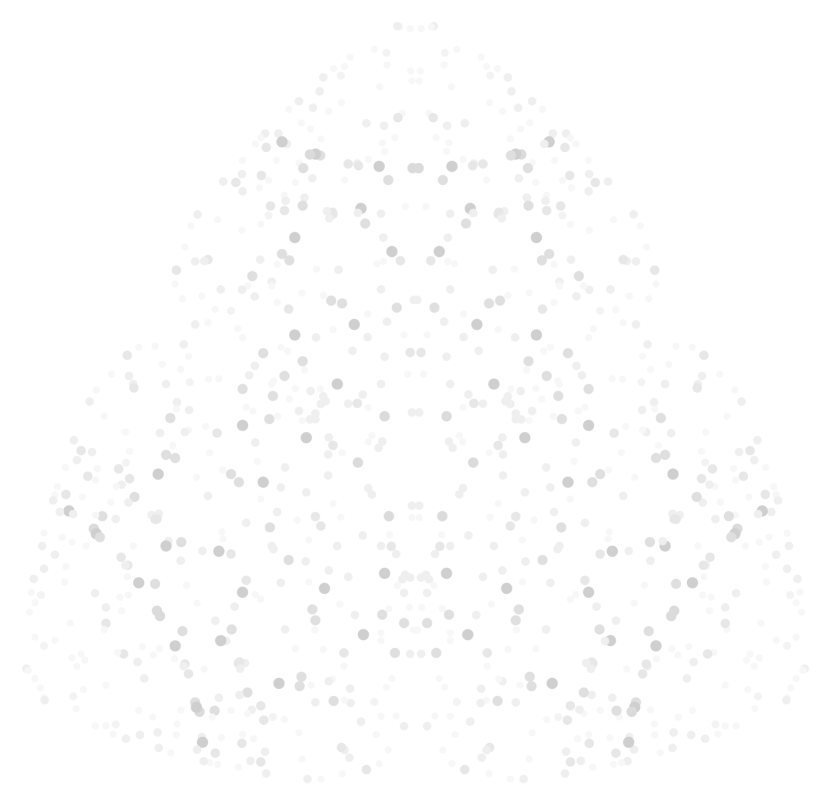
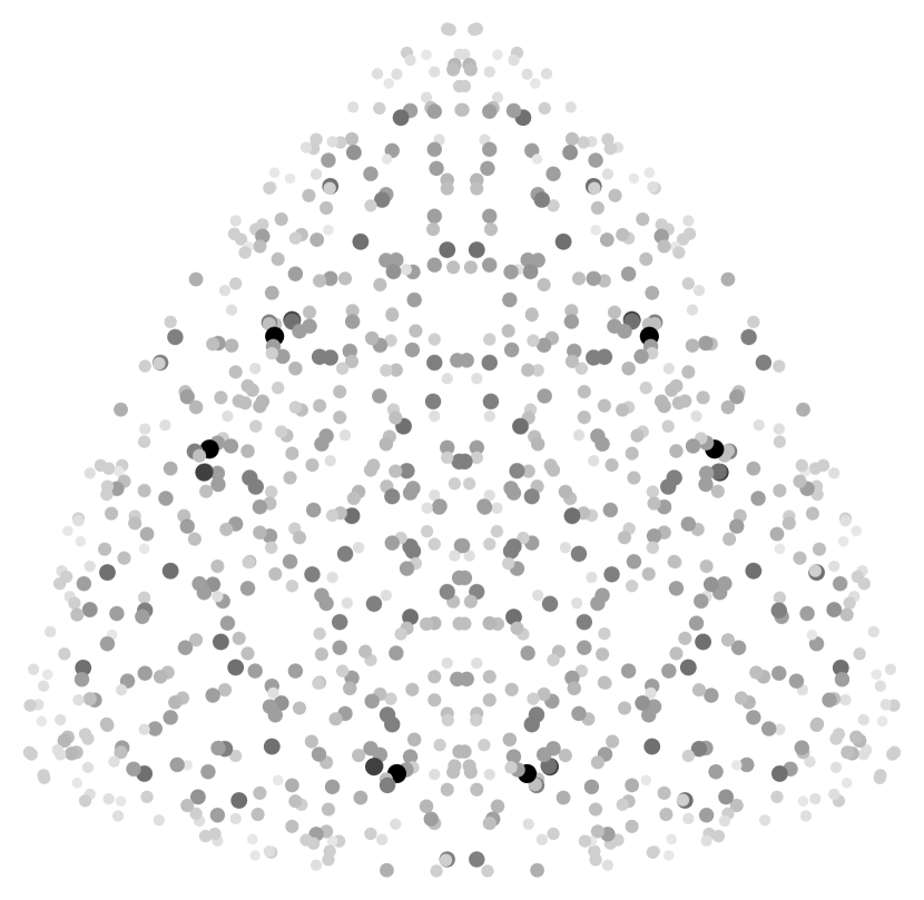
Figure 1.1. Weighted points on the sphere for $N=1716099$ and $N=1707035$

Remark 1.10 (Bias).

The term $L(1,\chi_{-N})N^{1/2}$ corresponds to the number of terms in the sum by a classical result of Gauss, whereas, $(\log N)^{k-1}$ is the average of the $k$-th divisor function. The shape of $\mathfrak{b}(N)$ is biased towards integers $N$ having many prime divisors $p\equiv 1\left(\textnormal{mod}\ 4\right)$ below $\log N$. It is possible to combine this with the work of Granville–Soundararajan [30, Theorem 5b], to find infinitely many $N$ such that

$$\sharp\{\mathbf{x}\in\mathbb{N}^{6}:(x_{1}x_{2})^{2}+(x_{3}x_{4})^{2}+(x_{5}x_{6})^{2}=N\}\gg(\log\log N)^{5/2}(\log N)^{3}N^{1/2}.$$

This is in constrast with the typical size, which is $(\log N)^{3}N^{1/2}$ because $L(1,\chi_{-N})$ and $\mathfrak{b}(N)$ possess a limiting distribution due to the work of Chowla–Erdős [15] and Erdős–Wintner [24].

The bias is illustrated in the three-dimensional plots in Figure 1.1. They depict points $\mathbf{x}\in\mathbb{N}^{3}$ with $\sum_{i=1}^{3}x_{i}^{2}=N$, where each $\mathbf{x}$ is colored based on the magnitude of $\prod_{i=1}^{3}\tau(x_{i})$. The equations respectively have $960$ and $936$ solutions in $\mathbb{N}^{3}$. Among the six primes that divide $1716099$, only one is $1\left(\textnormal{mod}\ 4\right)$. However, in the factorization of $1707035$, four primes are involved, and all except one are $1\left(\textnormal{mod}\ 4\right)$.

The ideas behind the proof of Theorem 1.9 are not specific to sums of three squares. We generalise the results to equations without specific shape, with the only provision that they have enough variables compared to the degree. The end result is to study multiplicative functions over the coordinates of integer solutions of these Diophantine equations. Problems of this type have been considered by Cook–Magyar [17] and Yamagishi [56] in the case of the von Mangoldt function.

Theorem 1.11.

Fix any $s>0$ and assume that $f:\mathbb{N}\to[0,\infty)$ is a multiplicative function satisfying $\tau(m)^{-s}\leqslant f(m)\leqslant\tau(m)^{s}$ for all $m$, where $\tau$ is the divisor function. Assume that $F\in\mathbb{Z}[x_{0},\ldots,x_{n}]$ is a smooth homogeneous polynomial of degree $d$ with $n\geqslant 4+(d-1)2^{d}$ such that $F=0$ has a non-zero integer solution. There exists $\epsilon_{F}>0$ that depends only on $F$ such that for all $B\geqslant 1$ one has

$$\sum_{\begin{subarray}{c}\mathbf{x}\in(\mathbb{Z}\setminus\{0\})^{n+1}\\ \max|x_{i}|\leqslant B,F(\mathbf{x})=0\end{subarray}}f(|x_{0}\cdots x_{n}|)\asymp B^{n+1-d}\left\{\exp\Big{(}(n+1)\sum_{p\leqslant B}\frac{(f(p)-1)}{p}\Big{)}+O(B^{-\epsilon_{F}})\right\},$$

where the implied constants depend at most on $F$ and $s$.

The proof is based on Birch’s circle method [7]. The term $B^{n+1-d}$ represents the number of terms in the sum over $\mathbf{x}$. It will be clear from the proof that the assumption $f(m)\geqslant\tau(m)^{-s}$ is only needed for the lower bound.

1.3. Application to classical averages

Nair and Tenenbaum proved upper bounds for the average of arithmetic functions evaluated over values of polynomials in [44]. Such sums are omnipresent in number theory: their work was crucial in many different problems. Examples include

• Equidistribution of CM points ([37]),

• Manin’s conjecture for counting rational points on surfaces ([13], [12]),

• Mass equidistribution ([33]),

• Unit fractions ([23]).

Such sums are of type (1.1) as can be seen by taking $\chi$ to be the indicator function of an interval and $c_{a}$ to be the value of the polynomial at an integer $a$. However, (1.1) also covers any polynomial in any number of variables. In §7 we shall prove Theorems 1.16 and 1.17. These results respectively give matching upper and lower bounds for

$$\sum_{\begin{subarray}{c}\mathbf{x}\in\mathbb{Z}^{n}\cap\mathcal{R}\\ Q(\mathbf{x})\neq 0\end{subarray}}f(|Q(\mathbf{x})|),$$ (1.4)

where $\mathcal{R}$ is a bounded subset of $\mathbb{R}^{n}$ and $Q(\mathbf{x})$ is an arbitrary polynomial in any number of variables. This is straightforward for polynomials without too many singularities but when $Q$ is very singular there is high probability that a small power of a prime divides its values. The new ingredient needed is an estimate by Pierce–Schindler–Wood [45, Lemma 4.10] giving elementary proofs to statements regarding the Igusa zeta function.

We state one of the corollaries first. For $k,m\in\mathbb{N}$ denote the number of representations of $m$ as the product of $k$ natural numbers by $\tau_{k}(m)$.

Theorem 1.12.

Let $k\geqslant 2,n\geqslant 1$ be arbitrary integers, let $\ell$ be any positive real number and let $Q$ be an integer irreducible polynomial in $n$ variables. Then for all $X\geqslant 2$ we have

$$X^{n}(\log X)^{k^{\ell}-1}\ll\sum_{\begin{subarray}{c}\mathbf{x}\in(\mathbb{Z}\cap[-X,X])^{n}\\ Q(\mathbf{x})\neq 0\end{subarray}}\tau_{k}(|Q(\mathbf{x})|)^{\ell}\ll X^{n}(\log X)^{k^{\ell}-1}.$$

Remark 1.13 (Previously known cases).

Erdős [25] dealt with the case $\ell=n=1,k=2$ and Linnik [41] with $n=1$, all $\ell,k\geqslant 1$ and $\deg(Q)=1$. Later, Delmer [19] worked in the cases when $\ell\geqslant 1,k=2,Q$ is irreducible and $n=1$, Nair–Tenenbaum [44] for all $\ell,k,Q$ and when $n=1$, and de la Bretèche–Browning [10] whenever $n\geqslant 2,\ell\geqslant 1,k\geqslant 1$ and $Q$ is homogeneous. Asymptotics for the divisor function over the values of polynomials in more than one variable have been achieved by various authors, see, for example the work of de la Bretèche–Browning [11], Zhou–Ding [57] and the list of references therein. It is worth mentioning that in the case $k=2,\ell=1$ and $Q$ a single irreducible polynomial in one variable, only the cases corresponding to linear and quadratic polynomials are known to satisfy an asymptotic, see the work of Hooley [34] and Bykovskiĭ [14].

Theorem 1.12 follows directly from our next two results. Denote

$$\varrho_{Q}(q):=\frac{\sharp\{\mathbf{y}\in(\mathbb{Z}/q\mathbb{Z})^{n}:Q(\mathbf{y})\equiv 0\left(\textnormal{mod}\ q\right)\}}{q^{n}}$$

for any $Q\in\mathbb{Z}[x_{1},\ldots,x_{n}]$ and $q\in\mathbb{N}$.

Definition 1.14.

Let $\mathcal{D}\subset\mathbb{R}^{n}$ be bounded. We let

$$X(\mathcal{D}):=\sup\left\{\max_{1\leqslant i\leqslant n}|x_{i}|:\mathbf{x}\in\mathcal{D}\right\}.$$

Definition 1.15 (A class of functions).

Fix $A\geqslant 1,\epsilon>0,C>0$. The set $\mathcal{M}(A,\epsilon,C)$ of functions $f:\mathbb{N}\rightarrow[0,\infty)$ is defined by the property that for all coprime $m,n$ one has

$$f(mn)\leqslant f(m)\min\{A^{\Omega(n)},Cn^{\epsilon}\}.$$

Theorem 1.16.

Fix $A\geqslant 1$ and let $\mathcal{D}$ be a bounded set. Let $Q$ be an arbitrary non-constant integer polynomial in $n$ variables without repeated polynomial factors over $\mathbb{Q}$ and let $f$ be a function such that for every $\epsilon>0$ there exists $C>0$ for which $f\in\mathcal{M}(A,\epsilon,C)$. Then there exists a positive constant $\epsilon_{Q}$ that depends on $Q$ such that

$$\sum_{\begin{subarray}{c}\mathbf{x}\in\mathbb{Z}^{n}\cap\mathcal{D}\\ Q(\mathbf{x})\neq 0\end{subarray}}f(|Q(\mathbf{x})|)\ll X(\mathcal{D})^{n}(\log 2X(\mathcal{D}))^{-r}\sum_{\begin{subarray}{c}a\leqslant X(\mathcal{D})^{n}\end{subarray}}f(a)\varrho_{Q}(a)+X(\mathcal{D})^{n-\epsilon_{Q}},$$

where $r$ denotes the number of distinct irreducible polynomial factors of $Q$ over $\mathbb{Q}$ and the implied constant depends at most on $A,f,n$ and $Q$.

For the corresponding lower bound to hold it is necessary that $\mathcal{D}$ is not too small; this explains the condition on $\mathcal{D}$ in our next result:

Theorem 1.17.

Keep the notation and assumptions of Theorem 1.16. Assume, in addition, that $\mathcal{D}$ contains an open sphere of radius at least $X\geqslant 1$ and that $f:\mathbb{N}\to[0,\infty)$ is a multiplicative function such that

$$\textrm{ for \ each }\ T\geqslant 1\ \textrm{ one \ has }\ \inf\{f(m):\Omega(m)\leqslant T\}>0.$$ (1.5)

Then there exists a positive constant $\theta_{Q}$ that depends on $Q$ such that

$$\sum_{\begin{subarray}{c}\mathbf{x}\in\mathbb{Z}^{n}\cap\mathcal{D}\\ Q(\mathbf{x})\neq 0\end{subarray}}f(|Q(\mathbf{x})|)\gg X^{n}(\log 2X)^{-r}\sum_{\begin{subarray}{c}a\leqslant X\end{subarray}}f(a)\varrho_{Q}(a)+O(X^{n-\theta_{Q}}),$$

where the implied constants depend at most on $A,f,n$ and $Q$.

Notation.

For a non-zero integer $m$ define

$$\Omega(m):=\sum_{p\mid m}v_{p}(m),$$

where $v_{p}$ is the standard $p$-adic valuation. Define $P^{+}(m)$ and $P^{-}(m)$ respectively to be the largest and the smallest prime factor of a positive integer $m$ and let $P^{+}(1)=1$ and $P^{-}(1)=+\infty$. For a real number $x$ we reserve the notation $[x]$ for the largest integer not exceeding $x$. Throughout the paper we use the standard convention that empty products are set equal to $1$. Throughout the paper we shall also make use of the convention that when iterated logarithm functions $\log t,\log\log t$, etc., are used, the real variable $t$ is assumed to be sufficiently large to make the iterated logarithm well-defined.

The following constants and functions are recurring throughout the paper:

Symbols	First appearance
$F:\mathbb{N}\to[0,\infty)$	Lemma 2.1
$c_{0},c_{1},c_{2}$	Lemma 2.1
$C,C^{\prime}$	Lemma 2.3
$G:\mathbb{N}\to[0,\infty)$	Lemma 2.4
$r$	Lemma 2.11
$\kappa,\lambda_{1},\lambda_{2},B,K$	Definition 3.1
$h:\mathbb{N}\to[0,\infty)$	Definition 3.1
$\mathcal{A},T,\chi_{T}$	Equations (3.4)-(3.5)
$C_{d}(T),M,M(T)$	Definition 3.5
$\theta,\xi$	Definition 3.5
$A,\mathcal{M}(A,\epsilon,C)$	Definition 1.15
$\alpha$, $\tilde{B}$	Equation (3.8)
$\eta_{1},\eta_{2},\eta_{3}$	Equation (3.9)
$Z$	Equation (3.10)
$b_{a},c_{a},d_{a}$	Equations (3.11)-(3.13)

Acknowledgements.

Part of the work in §§2-3 was completed while ES and CP were at Leiden University in $2016$. The work in the remaining sections started during the research stay of SC, PK and CP during the workshop Problèmes de densité en Arithmétique at CIRM Luminy in $2023$. We would like to thank the organisers Samuele Anni, Peter Stevenhagen and Jan Vonk. We thank Levent Alpöge, Robert J. Lemke Oliver and Frank Thorne for useful discussions on §5.1. PK gratefully acknowledges the support of Dr. Max Rössler, the Walter Haefner Foundation and the ETH Zürich Foundation. Part of the work of SC was supported by the National Science Foundation under Grant No. DMS-1928930, while the author was in residence at the MSRI in Spring 2023.

Structure of the paper

Section 2 consists of a series of lemmas that will be used to prove Theorem 3.8. The lemmas that do not rely on sieve theory are structured as follows:

while the following lemmas are independent and rely on sieve theory:

In §3 we prove our main result, Theorem 3.8, which is a general upper bound. In §4 we give matching general lower bounds when the arithmetic function $f$ stays away from $0$. Sections 5.1-5.2 respectively contain the proofs of Theorems 1.1 and 1.5 on the $6$-rank. In §5.3 we prove Theorem 5.2 that provides tail bounds for the probability of large values of additive functions in the general setting of Theorem 3.8. This is then applied in Sections 5.4-5.5 and 5.6 to prove Theorems 1.6-1.7 and 1.8 respectively on $h_{3}$, $S_{5}$ and $S_{3}$ extensions. Sections 6.1-6.6 contain the proof of Theorem 6.1 on sums of three squares; this is more general than Theorem 1.9. The proof of Theorem 1.11 on general Diophantine equations is located in §6.7. Lastly, in §7.2 and §7.3 we prove respectively Theorems 1.16 and 1.17 on averages of arithmetic functions over values of arbitrary polynomials. They are then applied in §7.4 to prove Theorem 1.12.

2. Preliminary lemmas

2.1. Required estimates for Theorem 3.8

The work of [48, Lemma 1] gives an upper bound on the density of integers all of whose prime factors are relatively small. We shall need a variation of this result where the integers are weighted by a multiplicative function. In the applications it will be important that the bound is of the form $O(x^{o(1)}z^{-c})$ for some positive constant $c$.

Lemma 2.1.

Fix any positive real numbers $c_{0},c_{1},c_{2}$ and assume that $F:\mathbb{N}\to[0,\infty)$ is a multiplicative function such that

$$F(p^{e})\leqslant\min\left\{\frac{c_{0}}{p},\frac{p^{c_{1}}}{p^{ec_{2}}}\right\}$$ (2.1)

for all primes $p$ and $e\geqslant 1$. Define

$$c:=\min\left\{\frac{c_{2}}{2},\frac{1}{1+[2c_{1}/c_{2}]}\right\}\ \textrm{ and }\ c^{\prime}:=\frac{c+2(c_{0}+c)}{c}.$$

Then for all $x,z\geqslant 2$ we have

$$\sum_{\begin{subarray}{c}n\in\mathbb{N}\cap(z,x]\\ p\mid n\Rightarrow p\leqslant(\log x)(\log\log x)\end{subarray}}F(n)\ll z^{-c}\exp\left(\frac{c^{\prime}\log x}{(\log\log x)^{1/2}}\right),$$

where the implied constant is absolute.

Proof.

Let $c_{4}$ be a positive constant that will be optimised later. Then the sum over $n$ is

$$\leqslant\frac{1}{z^{c_{4}}}\sum_{\begin{subarray}{c}n\leqslant x\\ p\mid n\Rightarrow p\leqslant y\end{subarray}}F(n)n^{c_{4}},$$

where $y=(\log x)(\log\log x)$. By Rankin’s trick we get the following bound for any $\delta>0$:

$$\leqslant\frac{x^{\delta}}{z^{c_{4}}}\sum_{\begin{subarray}{c}n\in\mathbb{N}\\ p\mid n\Rightarrow p\leqslant y\end{subarray}}F(n)\frac{n^{c_{4}}}{n^{\delta}}=\frac{x^{\delta}}{z^{c_{4}}}\prod_{p\leqslant y}\left(1+\sum_{e\geqslant 1}F(p^{e})p^{e(c_{4}-\delta)}\right).$$

For an auxiliary positive integer $e_{0}$ we shall control the contribution of the range $e\leqslant e_{0}$ and $e>e_{0}$ using the bounds $F(p^{e})\leqslant c_{0}/p$ and $F(p^{e})\leqslant p^{c_{1}-ec_{2}}$ respectively. Assume that $c_{4}\geqslant\delta$ so that the contribution of the former range contributes

$$\leqslant 1+\sum_{e=1}^{e_{0}}\frac{c_{0}}{p}\frac{p^{ec_{4}}}{p^{e\delta}}\leqslant 1+c_{0}e_{0}p^{e_{0}(c_{4}-\delta)-1}.$$

Now assume that $c_{4}e_{0}\leqslant 1$ so that the bound becomes

$$\leqslant 1+\frac{c_{0}}{c_{4}}p^{-\delta e_{0}}\leqslant 1+\frac{c_{0}}{c_{4}}p^{-\delta}\leqslant 1+\frac{c_{0}}{c_{4}}\frac{1}{p^{\delta}-1}.$$

The remaining range contributes

$$\leqslant p^{c_{1}}\sum_{e\geqslant 1+e_{0}}p^{e(c_{4}-\delta-c_{2})}.$$

Making the additional assumption that $c_{4}\leqslant\frac{1}{2}c_{2}$ we can bound this by

$$\leqslant p^{c_{1}}\sum_{e\geqslant 1+e_{0}}p^{-e(\delta+c_{2}/2)}\leqslant\frac{p^{c_{1}}}{p^{e_{0}(\delta+c_{2}/2)}}\sum_{j=1}^{\infty}\frac{1}{p^{j(\delta+c_{2}/2)}}\leqslant\frac{p^{c_{1}}}{p^{e_{0}c_{2}/2}}\frac{1}{p^{\delta}-1}.$$

Further assuming that $2c_{1}\leqslant e_{0}c_{2}$ shows that this is $\leqslant\frac{1}{p^{\delta}-1}$. Putting the bounds together leads to

$$1+\sum_{e\geqslant 1}F(p^{e})p^{e(c_{4}-\delta)}\leqslant 1+\frac{c_{0}+c_{4}}{c_{4}}\frac{1}{p^{\delta}-1},$$

subject to the conditions

$$\delta\leqslant c_{4},c_{4}e_{0}\leqslant 1,c_{4}\leqslant\frac{c_{2}}{2},\frac{2c_{1}}{c_{2}}\leqslant e_{0}.$$

Putting $e_{0}=1+[2c_{1}/c_{2}]$ shows that these conditions are met for any $\delta\in(0,c_{4})$ where

$$c_{4}:=\min\left\{\frac{c_{2}}{2},\frac{1}{1+[2c_{1}/c_{2}]}\right\}=c.$$

Hence, the overall bound becomes

$$\frac{x^{\delta}}{z^{c_{4}}}\prod_{p\leqslant y}\left(1+\frac{c_{0}+c_{4}}{c_{4}}\frac{1}{p^{\delta}-1}\right)\leqslant\frac{x^{\delta}}{z^{c_{4}}}\prod_{p\leqslant y}\left(1+\frac{1}{p^{\delta}-1}\right)^{\frac{c_{0}+c_{4}}{c_{4}}}\leqslant z^{-c_{4}}\exp\left(\delta(\log x)+\frac{c_{0}+c_{4}}{c_{4}}T\right),$$

where

$$T:=\sum_{p\leqslant y}\frac{1}{p^{\delta}-1}\leqslant\frac{1}{\delta}\sum_{p\leqslant y}\frac{1}{\log p}\leqslant\frac{1}{\delta}\frac{2y}{(\log y)^{2}},$$

owing to the inequality $\mathrm{e}^{t}-1\geqslant t$ with $t=\delta\log p$ and the prime number theorem. Putting $\delta=(\log\log x)^{-1/2}$ we see that when $y=(\log x)(\log\log x)$ one gets the bound

$$z^{-c_{4}}\exp\left(\frac{\log x}{(\log\log x)^{1/2}}+\frac{(c_{0}+c_{4})}{c_{4}}(\log\log x)^{1/2}\frac{2(\log x)(\log\log x)}{(\log\log x)^{2}}\right),$$

which is sufficient. ∎

Lemma 2.2.

Keep the setting of Lemma 2.1 and fix any $\beta_{0}>0$. For all $T\geqslant 2$ with $\log T>4\beta_{0}/c_{2}$, for all $A>1,c\in\mathbb{N}$, and for any $\beta>0$ with

$$\beta\leqslant\min\left\{\frac{c_{2}}{2},\frac{\beta_{0}}{\log T}\right\},$$

the product

$$\prod_{\begin{subarray}{c}p\leqslant T\\ p\nmid c\end{subarray}}\Big{(}1+\sum_{\begin{subarray}{c}i\geqslant 1\\ j\geqslant 0\end{subarray}}\min\{C^{\prime}p^{(i+j)c_{2}/2},A^{i+j}\}F(p^{i+j})(p^{\beta i}-p^{\beta(i-1)})\Big{(}\frac{\mathds{1}[p>c_{0}]}{(1-F(p))}+\mathds{1}[p\leqslant c_{0}]\Big{)}\Big{)}$$

is $O(\mathrm{e}^{\nu\beta\log T})$, where $\nu$ is a positive constant that depends at most on $\beta_{0}$, $c_{i}$ and $A$. Furthermore, the implied constant depends at most on $A,C^{\prime},c_{0},c_{1}$ and $c_{2}$.

Proof.

Define $p_{0}$ to be the least prime satisfying $2A\leqslant p_{0}^{c_{2}/4}$. We will bound the sum over $i,j$ for every individual prime $p\geqslant p_{0}$ and in the end we shall piece the bounds together for all primes $p\leqslant T$.
Step (1). We start with the contribution of large $i$, in which case the bound $F(p^{e})\leqslant p^{c_{1}-ec_{2}}$ and the crude estimate $p^{\beta i}-p^{\beta(i-1)}\leqslant p^{\beta i}$ will suffice. Define

$$i_{1}:=1+\left[\frac{4(5+c_{1})}{c_{2}}\right].$$

The contribution of $i\geqslant i_{1}$ is

$$\leqslant\sum_{i\geqslant i_{1}}A^{i}p^{\beta i}\sum_{j\geqslant 0}A^{j}F(p^{i+j})\leqslant p^{c_{1}}\sum_{i\geqslant i_{1}}A^{i}p^{(\beta-c_{2})i}\sum_{j\geqslant 0}(Ap^{-c_{2}})^{j}\leqslant 2p^{c_{1}}\sum_{i\geqslant i_{1}}(Ap^{(\beta-c_{2})})^{i}$$

because $Ap^{-c_{2}}\leqslant 1/2$, a fact that follows from $p\geqslant p_{0}$. Now we use the assumptions $\beta\leqslant c_{2}/2$ and $2A\leqslant p_{0}^{c_{2}/4}\leqslant p^{c_{2}/4}$ to see that $Ap^{(\beta-c_{2})}\leqslant Ap^{-c_{2}/2}\leqslant 1/2$. Hence,

$$2p^{c_{1}}\sum_{i\geqslant i_{1}}(Ap^{(\beta-c_{2})})^{i}\leqslant 4p^{c_{1}}(Ap^{(\beta-c_{2})})^{i_{1}}\leqslant 4p^{c_{1}-i_{1}c_{2}/4}\leqslant p^{2+c_{1}-i_{1}c_{2}/4}.$$

This is $\leqslant p^{-3}$ because our choice for $i_{1}$ makes sure that $5+c_{1}\leqslant i_{1}c_{2}/4.$ We have thus shown that for all $p\geqslant p_{0}$ one has

$$\sum_{\begin{subarray}{c}i\geqslant i_{1}\\ j\geqslant 0\end{subarray}}A^{i+j}F(p^{i+j})(p^{\beta i}-p^{\beta(i-1)})\leqslant p^{-3}.$$

Step (2). Let us now bound the contribution of the $i,j$ that satisfy

$$1\leqslant i<i_{1}\ \ \textrm{ and }\ \ i+j\geqslant i_{1}.$$

We have

$$\sum_{i=1}^{i_{1}-1}\sum_{j\geqslant i_{1}-i}A^{i+j}F(p^{i+j})(p^{\beta i}-p^{\beta(i-1)})\leqslant p^{c_{1}}\sum_{i=1}^{i_{1}-1}A^{i}p^{-ic_{2}}(p^{\beta i}-p^{\beta(i-1)})\sum_{j\geqslant i_{1}-i}(Ap^{-c_{2}})^{j}.$$

Using the inequality $Ap^{-c_{2}}\leqslant 1/2$ to bound the sum over $j$ results in the inequality

$$\leqslant 2p^{c_{1}}\sum_{i=1}^{i_{1}-1}A^{i}p^{-ic_{2}}(p^{\beta i}-p^{\beta(i-1)})(Ap^{-c_{2}})^{i_{1}-i}=2p^{c_{1}}A^{i_{1}}p^{-c_{2}{i_{1}}}\sum_{i=1}^{i_{1}-1}(p^{\beta i}-p^{\beta(i-1)}),$$

which is at most $2p^{c_{1}}(Ap^{(\beta-c_{2})})^{i_{1}}$ that has been previously shown to be at most $\leqslant 1/p^{3}$.

We have thus proved that for all $p\geqslant p_{0}$ one has

$$\sum_{\begin{subarray}{c}1\leqslant i<i_{1}\\ j\geqslant i_{1}-i\end{subarray}}A^{i+j}F(p^{i+j})(p^{\beta i}-p^{\beta(i-1)})\leqslant p^{-3}.$$

Step (3). It remains to study the contribution of cases with $i+j<i_{1}$. For these we use the assumption $F(p^{e})\leqslant c_{0}/p$ that leads to the bound

$$\leqslant\frac{c_{0}}{p}\sum_{\begin{subarray}{c}i\geqslant 1,j\geqslant 0\\ i+j<i_{1}\end{subarray}}A^{i+j}(p^{\beta i}-p^{\beta(i-1)})\leqslant\frac{c_{0}}{p}\sum_{1\leqslant i<i_{1}}(2A)^{i}(p^{\beta i}-p^{\beta(i-1)})\sum_{\begin{subarray}{c}0\leqslant j<i_{1}-i\end{subarray}}(2A)^{j}.$$

Now since $A>1$ we have $2A>2$. For all $m\geqslant 1$ we have

$$1+(2A)+(2A)^{2}+\ldots+(2A)^{m-1}\leqslant\frac{(2A)^{m}}{2A-1}\leqslant(2A)^{m}.$$

This gives the bound

$$\leqslant\frac{c_{0}}{p}\sum_{1\leqslant i<i_{1}}(2A)^{i}(p^{\beta i}-p^{\beta(i-1)})(2A)^{i_{1}-i}=\frac{c_{0}(2A)^{i_{1}}}{p}\sum_{1\leqslant i<i_{1}}(p^{\beta i}-p^{\beta(i-1)})\leqslant\frac{c_{0}(2A)^{i_{1}}}{p}(p^{\beta i_{1}}-1).$$

The assumption $\beta\log T\leqslant\beta_{0}$ shows that $\beta i_{1}\log T\leqslant\beta_{0}(1+\frac{4(5+c_{1})}{c_{2}})$, hence, for primes $p\leqslant T$ we infer $\beta i_{1}\log p\leqslant\beta_{0}(1+\frac{4(5+c_{1})}{c_{2}})$. On the other hand, the function $(-1+\mathrm{e}^{t})/t$ is bounded in the interval $0\leqslant t\leqslant\beta_{0}(1+\frac{4(5+c_{1})}{c_{2}})$, thus,

$$p^{\beta i_{1}}-1=\exp((\log p)\beta i_{1})-1\leqslant\beta_{1}(\log p)\beta i_{1},$$

for a positive constant $\beta_{1}$ that depends on $\beta_{0}$ and $c_{1},c_{2}$. Thus, the contribution of cases with $i+j<i_{1}$ is

$$\leqslant\frac{c_{0}(2A)^{i_{1}}}{p}(p^{\beta i_{1}}-1)\leqslant\left\{c_{0}(2A)^{i_{1}}\beta_{1}\beta i_{1}\right\}\frac{\log p}{p}.$$

In conclusion, we saw that for all primes $p\in(p_{0},T]$ one has

$$\sum_{\begin{subarray}{c}i\geqslant 1\\ j\geqslant 0\end{subarray}}A^{i+j}F(p^{i+j})(p^{\beta i}-p^{\beta(i-1)})\leqslant 2p^{-3}+\left\{c_{0}(2A)^{i_{1}}\beta_{1}\beta i_{1}\right\}\frac{\log p}{p}.$$

Step (4). Using the last inequality with the bound $1+x_{p}\leqslant\exp(x_{p})$, valid for all $x_{p}\in\mathbb{R}$, shows that, once restricted in the range $p>\max\{p_{0},c_{0}\}$, the product in the lemma is

$$\leqslant\exp\Big{(}\sum_{\begin{subarray}{c}\max\{p_{0},c_{0}\}<p\leqslant T\\ p\nmid c\end{subarray}}(1-F(p))^{-1}\Big{(}2p^{-3}+\left\{c_{0}(2A)^{i_{1}}\beta_{1}\beta i_{1}\right\}\frac{\log p}{p}\Big{)}\Big{)}.$$

Ignoring the condition $p\nmid c$ will produce a larger bound. Using the inequality $F(p)\leqslant c_{0}/p$ we obtain

$$\ll\exp\Big{(}c_{0}(2A)^{i_{1}}\beta_{1}\beta i_{1}\sum_{\begin{subarray}{c}\max\{p_{0},c_{0}\}<p\leqslant T\end{subarray}}(1-F(p))^{-1}\frac{\log p}{p}\Big{)},$$

where the implied constant depends at most on $c_{0}$. Using the inequality $F(p)\leqslant c_{0}/p$ and the estimate $\sum_{p\leqslant y}(\log p)/p\ll\log y$ leads to

$$\sum_{\begin{subarray}{c}\max\{p_{0},c_{0}\}<p\leqslant T\end{subarray}}\frac{\log p}{(1-F(p))p}\leqslant\sum_{\begin{subarray}{c}\max\{p_{0},c_{0}\}<p\leqslant T\end{subarray}}\frac{\log p}{p}\left(1+O_{c_{0}}\left(\frac{c_{0}}{p}\right)\right)\ll O_{c_{0}}(1)+\log T,$$

where the implied constant is absolute. Hence, the previous bound becomes

$$\ll_{c_{0}}\exp\Big{(}c_{0}(2A)^{i_{1}}\beta_{1}\beta i_{1}\log T\Big{)}.$$

Since $i_{1}$ is a function of $c_{1}$ and $c_{2}$ we can thus write the bound as $\ll_{c_{0}}\exp(\nu\beta\log T)$ for some $\nu=\nu(\beta_{0},c_{0},c_{1},c_{2},A)$. To conclude the proof of the lemma we must deal with the contribution of the primes $p\leqslant\max\{p_{0},c_{0}\}$. Note that for every prime $p$ the corresponding factor in the product of the lemma is

$$\leqslant 1+\Big{(}\frac{1}{1-F(p)}+1\Big{)}\sum_{\begin{subarray}{c}i\geqslant 1\\ j\geqslant 0\end{subarray}}\min\{C^{\prime}p^{(i+j)c_{2}/2},A^{i+j}\}F(p^{i+j})p^{\beta i}.$$

Using the bound for $F$ in the assumptions of Lemma 2.1 and the bound $\beta\leqslant\beta_{0}/\log T$ we see that the sum over $i,j$ is at most

$$C^{\prime}p^{c_{1}}\sum_{i\geqslant 1}p^{(-c_{2}/2+\beta_{0}/\log T)i}\sum_{j\geqslant 0}p^{-jc_{2}/2}.$$

Our assumption $4\beta_{0}/c_{2}<\log T$ ensures that $\beta_{0}/\log T<c_{2}/4$, hence, we obtain the bound

$$C^{\prime}p^{c_{1}}\sum_{i\geqslant 1}p^{-ic_{2}/4}\sum_{j\geqslant 0}p^{-jc_{2}/2}\leqslant C^{\prime}p^{c_{1}}\sum_{i\geqslant 1}2^{-ic_{2}/4}\sum_{j\geqslant 0}2^{-jc_{2}/2}=O_{c_{2}}(C^{\prime}p^{c_{1}}).$$

Taking the product of this quantity over all primes $p\leqslant\max\{p_{0},c_{0}\}$ gives an implied constant that depends on $p_{0},c_{0},c_{1},c_{2}$ and $C^{\prime}$. Since $p_{0}=p_{0}(A,c_{2})$ we see that the implied constant also depends on $A$. ∎

Lemma 2.3.

Fix any positive constants $C,C^{\prime},\epsilon$ and assume that we are given a function $G:\mathbb{N}\to[0,\infty)$ such that for all coprime positive integers $a,b$ one has

$$G(ab)\leqslant G(a)\min\{C^{\Omega(b)},C^{\prime}b^{\epsilon}\}.$$

Then for all coprime positive integers $a,b$ we have $G(ab)\leqslant G(a)H(b)$, where $H$ is the multiplicative function defined as $H(p^{e})=\min\{C^{e},C^{\prime}p^{\epsilon e}\}$ for all $e\geqslant 1$ and primes $p$.

Proof.

We will prove this with induction on $\omega(b)$. When $\omega(b)=0$ then $b=1$, hence, the statement clearly holds. Assume that $k\geqslant 0$ and that the statement holds for all $b\in\mathbb{N}$ with $\omega(b)=k$. Now let $n,n^{\prime}$ be coprime and assume that $\omega(n)=k+1$. We shall show that $G(n^{\prime}n)\leqslant G(n^{\prime})H(n)$. Writing $n=p_{1}^{\alpha_{1}}\cdots p_{k}^{\alpha_{k}}p_{k+1}^{\alpha_{k+1}}$ where each $\alpha_{i}$ is strictly positive and the $p_{i}$ are distinct primes, we let $a=n^{\prime}p_{1}^{\alpha_{1}}\cdots p_{k}^{\alpha_{k}}$ and $b=p_{k+1}^{\alpha_{k+1}}$ so that

$$G(n^{\prime}n)=G(ab)\leqslant G(a)H(p_{k+1}^{\alpha_{k+1}})$$

by assumption. Now $a$ can be written as $n^{\prime}$ multiplied by an integer that is coprime to $n^{\prime}$ and with exactly $k$ distinct prime factors, thus, our inductive hypothesis shows that

$$G(a)\leqslant G(n^{\prime})\prod_{i=1}^{k}H(p_{i}^{\alpha_{i}}).$$

Combining the two inequalities gives $G(n^{\prime}n)\leqslant G(n^{\prime})\prod_{i\leqslant k+1}H(p_{i}^{\alpha_{i}})=G(n^{\prime})H(n)$.∎

Lemma 2.4.

Keep the setting of Lemma 2.1, fix any $C>1$ and $C^{\prime}>0$ and assume that $G:\mathbb{N}\to[0,\infty)$ is a function that satisfies

$$G(ab)\leqslant G(a)\min\{C^{\Omega(b)},C^{\prime}b^{c_{2}/2}\}$$ (2.2)

for all coprime positive integers $a,b$. Fix any positive real number $\beta_{0}$. For any $\Upsilon,\Psi\geqslant 2$ and $\varpi>0$ satisfying

$$\varpi\leqslant\min\left\{\frac{c_{2}}{2}\log\Psi,\beta_{0}\right\}$$

we have

$$\sum_{\begin{subarray}{c}a>\Upsilon\\ P^{+}(a)<\Psi\end{subarray}}F(a)G(a)\prod_{\begin{subarray}{c}c_{0}<p\\ p\mid a\end{subarray}}(1-F(p))^{-1}\ll\exp\left(-\varpi\frac{\log\Upsilon}{\log\Psi}\right)\sum_{\begin{subarray}{c}n\in\mathbb{N}\\ P^{+}(n)<\Psi\end{subarray}}F(n)G(n)\prod_{\begin{subarray}{c}c_{0}<p\\ p\mid n\end{subarray}}(1-F(p))^{-1},$$

where the implied constant depends at most on $C,C^{\prime},\beta_{0}$ and $c_{i}$.

Proof.

Define $\beta:=\varpi/\log\Psi$. The sum is at most

$$\sum_{P^{+}(a)<\Psi}F(a)G(a)\prod_{\begin{subarray}{c}c_{0}<p\\ p\mid a\end{subarray}}(1-F(p))^{-1}\left(\frac{a}{\Upsilon}\right)^{\beta}.$$

Now define the multiplicative function $\psi_{\beta}:\mathbb{N}\to\mathbb{R}$ via the Dirichet convolution

$$m^{\beta}=\sum_{\begin{subarray}{c}d\in\mathbb{N}\\ d\mid m\end{subarray}}\psi_{\beta}(d),\ \ \ m\in\mathbb{N}.$$

Writing $n=a/d$ we obtain

$$\Upsilon^{-\beta}\sum_{\begin{subarray}{c}d\in\mathbb{N}\\ P^{+}(d)<\Psi\end{subarray}}\psi_{\beta}(d)\sum_{\begin{subarray}{c}n\in\mathbb{N}\\ P^{+}(n)<\Psi\end{subarray}}F(nd)G(nd)\prod_{\begin{subarray}{c}c_{0}<p\\ p\mid nd\end{subarray}}(1-F(p))^{-1}.$$

Now factor $n=n_{0}n_{1}$, where $\gcd(n_{1},d)=1$ and $n_{0}$ is only divisible by primes dividing $d$. Then the sum over $d$ and $n$ becomes

$$\sum_{\begin{subarray}{c}d\in\mathbb{N}\\ P^{+}(d)<\Psi\end{subarray}}\psi_{\beta}(d)\sum_{\begin{subarray}{c}\mathbf{n}\in\mathbb{N}^{2},\ P^{+}(n_{0}n_{1})<\Psi\\ p\mid n_{0}\Rightarrow p\mid d\\ \gcd(n_{1},d)=1\end{subarray}}F(n_{0}n_{1}d)G(n_{0}n_{1}d)\prod_{\begin{subarray}{c}c_{0}<p\\ p\mid n_{0}n_{1}d\end{subarray}}(1-F(p))^{-1}.$$

Our assumptions on $G$ together with Lemma 2.3 ensure that $G(n_{0}n_{1}d)\leqslant G(n_{1})H(n_{0}d)$, where $H$ is the multiplicative function given by $H(p^{e})=\min\{C^{e},C^{\prime}p^{ec_{2}/2}\}$ for $e\geqslant 1$ and primes $p$. Together with the multiplicativity of $F$ we obtain the bound

$$\Upsilon^{-\beta} \sum_{\begin{subarray}{c}n_{1}\in\mathbb{N}\\ P^{+}(n_{1})<\Psi\end{subarray}}F(n_{1})G(n_{1})\prod_{\begin{subarray}{c}c_{0}<p\\ p\mid n_{1}\end{subarray}}(1-F(p))^{-1}$$

$$\times \sum_{\begin{subarray}{c}n_{0},d\in\mathbb{N},P^{+}(d)<\Psi\\ p\mid n_{0}\Rightarrow p\mid d\\ \gcd(d,n_{1})=1\end{subarray}}F(n_{0}d)H(n_{0}d)\psi_{\beta}(d)\prod_{\begin{subarray}{c}c_{0}<p\\ p\mid d\end{subarray}}(1-F(p))^{-1}.$$

It is easy to see that $\psi_{\beta}(p^{m})=p^{\beta m}-p^{\beta(m-1)}$ for all $m\geqslant 1$ and primes $p$. We can use this to write the sum over $n_{0},d$ as an Euler product. The Euler product is of the type covered by Lemma 2.2 as can be seen by taking $A=C,c=n_{1}$ and $T=\Psi$. The assumption of the present lemma on the size of $\varpi$ implies that the assumption of Lemma 2.2 on the size of $\beta$. Thus, the sum over $a$ in the lemma is

$$\ll\frac{\mathrm{e}^{\nu\beta\log\Psi}}{\Upsilon^{\beta}}\sum_{\begin{subarray}{c}n\in\mathbb{N}\\ P^{+}(n)<\Psi\end{subarray}}F(n)G(n)\prod_{\begin{subarray}{c}c_{0}<p\\ p\mid n\end{subarray}}(1-F(p))^{-1},$$

where $\nu=\nu(\beta_{0},c_{0},c_{1},c_{2},C)$ is positive and the implied constant depends at most on $C$ and $c_{i}$. Using the fact that $\varpi\leqslant\beta_{0}$, we can write

$$\mathrm{e}^{\nu\beta\log\Psi}=\mathrm{e}^{\nu\varpi}=O_{\beta_{0}}(1).$$

Finally, we have $\Upsilon^{-\beta}=\exp(-\varpi\log\Upsilon/\log\Psi)$. ∎

Lemma 2.5.

Keep the setting of Lemma 2.4 and define for any $V\geqslant 1$ the function

$$\mathcal{H}(V):=\sum_{\begin{subarray}{c}n\in\mathbb{N}\\ P^{+}(n)<V\end{subarray}}F(n)G(n)\prod_{\begin{subarray}{c}c_{0}<p\\ p\mid n\end{subarray}}(1-F(p))^{-1}.$$

For $V\geqslant 1$ and $\epsilon>0$ with $V^{\epsilon c_{2}/2}>2C$ and $V^{\epsilon}>c_{0}$ we have

$$\mathcal{H}(V)\ll\frac{\mathcal{H}(V^{\epsilon})}{\epsilon^{\nu_{1}}},$$

where $\nu_{1}=\nu_{1}(C,c_{0},c_{1},c_{2})$ is positive and the implied constant depends at most on $C$, $C^{\prime}$ and $c_{i}$.

Proof.

For a prime $p>V^{\epsilon}$ we have $p^{c_{2}/2}>2C$ due to the assumption $V^{\epsilon c_{2}/2}>2C$. Now let $j_{0}:=1+[4/c_{2}+2c_{1}/c_{2}]$ so that $j_{0}c_{2}\geqslant 4+2c_{1}$. Then $-j_{0}c_{2}/2\leqslant-c_{1}-2$, which can be combined with $p^{c_{2}/2}>2C$ to show that

$$(Cp^{-c_{2}})^{j_{0}}\leqslant p^{-j_{0}c_{2}/2}\leqslant p^{-c_{1}-2}.$$

By (2.1) and the fact that $C>1$ we see that

$$\sum_{j=1}^{\infty}C^{j}F(p^{j})\leqslant j_{0}C^{j_{0}}\frac{c_{0}}{p}+p^{c_{1}}\sum_{j=1+j_{0}}^{\infty}(Cp^{-c_{2}})^{j}\leqslant j_{0}C^{j_{0}}\frac{c_{0}}{p}+p^{c_{1}}2(Cp^{-c_{2}})^{j_{0}}\leqslant j_{0}C^{j_{0}}\frac{c_{0}}{p}+\frac{2}{p^{2}},$$

which is at most $\nu_{1}/p$, where $\nu_{1}$ is a positive constant that depends at most on $C$ and $c_{i}$. We infer that

$$\prod_{p\in(V^{\epsilon},V)}\!\left(1+\sum_{j=1}^{\infty}\frac{C^{j}F(p^{j})}{1-F(p)}\right)\leqslant\prod_{p\in(V^{\epsilon},V)}\!\left(1+\frac{\nu_{1}/p}{1-c_{0}/p}\right)\ll\prod_{p\in(V^{\epsilon},V)}\!\left(1+\frac{1}{p}\right)^{\nu_{1}}\!\!\ll\frac{1}{\epsilon^{\nu_{1}}},$$ (2.3)

with an implied constant that depends at most on $C$ and $c_{i}$.

We can now use (2.3) to bound $\mathcal{H}(V)$. Each positive integer $n$ can be written uniquely as $n=n_{0}n_{1}$, where $P^{+}(n_{0})\leqslant V^{\epsilon}$ and $P^{-}(n_{1})>V^{\epsilon}$. We have $G(n_{0}n_{1})\leqslant G(n_{0})C^{\Omega(n_{1})}$ by equation (2.2) and together with the multiplicativity of $F$ we obtain

$$\mathcal{H}(V)\leqslant\sum_{\begin{subarray}{c}n_{0}\in\mathbb{N}\\ P^{+}(n_{0})\leqslant V^{\epsilon}\end{subarray}}F(n_{0})G(n_{0})\prod_{\begin{subarray}{c}c_{0}<p\\ p\mid n_{0}\end{subarray}}(1-F(p))^{-1}\sum_{\begin{subarray}{c}n_{1}\in\mathbb{N}\\ P^{-}(n_{1})>V^{\epsilon}\\ P^{+}(n_{1})<V\end{subarray}}C^{\Omega(n_{1})}F(n_{1})\prod_{\begin{subarray}{c}c_{0}<p\\ p\mid n_{1}\end{subarray}}(1-F(p))^{-1}.$$

The assumption $V^{\epsilon}>c_{0}$ shows that every prime $p>V^{\epsilon}$ satisfies $p>c_{0}$, hence, the sum over $n_{1}$ equals

$$\prod_{V^{\epsilon}<p<V}\left(1+(1-F(p))^{-1}\sum_{j=1}^{\infty}C^{j}F(p^{j})\right).$$

Alluding to (2.3) and noting that the sum over $n_{0}$ equals $\mathcal{H}(V^{\epsilon})$ concludes the proof. ∎

Lemma 2.6.

Let $F$ be as in Lemma 2.1 and $G$ be as in Lemma 2.4. Fix any positive real number $\beta_{0}$. For sufficiently large $\Upsilon,\Psi\geqslant 2$ and for all $\varpi>0$ satisfying

$$\varpi\leqslant\min\left\{\frac{c_{2}}{2}\log\Psi,\beta_{0}\right\}$$

we have

$$\sum_{\begin{subarray}{c}a>\Upsilon\\ P^{+}(a)<\Psi\end{subarray}}F(a)G(a)\prod_{\begin{subarray}{c}c_{0}<p\\ p\mid a\end{subarray}}(1-F(p))^{-1}\ll\exp\left(-\varpi\frac{\log\Upsilon}{\log\Psi}\right)\sum_{\begin{subarray}{c}a\leqslant\Psi\end{subarray}}F(a)G(a)\prod_{\begin{subarray}{c}c_{0}<p\\ p\mid a\end{subarray}}(1-F(p))^{-1},$$

where the implied constant depends at most on $C,\beta_{0}$ and $c_{i}$.

Proof.

Taking $\Psi=\Upsilon^{\epsilon}$ and $\beta_{0}=\varpi=1$ in Lemma 2.4 shows that

$$\sum_{\begin{subarray}{c}a>\Upsilon\\ P^{+}(a)<\Upsilon^{\epsilon}\end{subarray}}F(a)G(a)\prod_{\begin{subarray}{c}c_{0}<p\\ p\mid a\end{subarray}}(1-F(p))^{-1}\ll\frac{\mathcal{H}(\Upsilon^{\epsilon})}{\exp(1/\epsilon)},$$

where the implied constant depends at most on $C$, $C^{\prime}$ and $c_{i}$. Taking a sufficiently small $\epsilon=\epsilon_{0}$ in terms of $C$ and $c_{i}$ makes the right-hand side be $\leqslant\mathcal{H}(\Upsilon^{\epsilon_{0}})/2$. Furthermore, by the definition of $\mathcal{H}$ we have

$$\mathcal{H}(\Upsilon^{\epsilon_{0}})\leqslant\sum_{\begin{subarray}{c}a\leqslant\Upsilon\\ P^{+}(a)<\Upsilon^{\epsilon_{0}}\end{subarray}}F(a)G(a)\prod_{\begin{subarray}{c}c_{0}<p\\ p\mid a\end{subarray}}(1-F(p))^{-1}+\sum_{\begin{subarray}{c}a>\Upsilon\\ P^{+}(a)<\Upsilon^{\epsilon_{0}}\end{subarray}}F(a)G(a)\prod_{\begin{subarray}{c}c_{0}<p\\ p\mid a\end{subarray}}(1-F(p))^{-1},$$

thus,

$$\mathcal{H}(\Upsilon^{\epsilon_{0}})\leqslant\sum_{\begin{subarray}{c}a\leqslant\Upsilon\end{subarray}}F(a)G(a)\prod_{\begin{subarray}{c}c_{0}<p\\ p\mid a\end{subarray}}(1-F(p))^{-1}+\frac{\mathcal{H}(\Upsilon^{\epsilon_{0}})}{2}.$$

Hence,

$$\mathcal{H}(\Upsilon^{\epsilon_{0}})\leqslant 2\sum_{\begin{subarray}{c}a\leqslant\Upsilon\end{subarray}}F(a)G(a)\prod_{\begin{subarray}{c}c_{0}<p\\ p\mid a\end{subarray}}(1-F(p))^{-1}.$$

Thus, by Lemma 2.5 we infer that

$$\mathcal{H}(\Psi)\ll\frac{\mathcal{H}(\Psi^{\epsilon_{0}})}{\epsilon_{0}^{\nu_{1}}}\ll\sum_{\begin{subarray}{c}a\leqslant\Psi\end{subarray}}F(a)G(a)\prod_{\begin{subarray}{c}c_{0}<p\\ p\mid a\end{subarray}}(1-F(p))^{-1}.$$

We conclude the proof by injecting this estimate into Lemma 2.4. ∎

Lemma 2.7.

Let $F$ be as in Lemma 2.1 and $G$ be as in Lemma 2.4. Fix any positive constant $\gamma$ and assume that for every prime $p$ we are given a constant $c(p)$ in the interval $[0,\gamma/p]$. Then for all $T\geqslant 1$ we have

$$\sum_{\begin{subarray}{c}a\leqslant T\end{subarray}}F(a)G(a)\prod_{p\mid a}(1+c(p))\leqslant 2^{\gamma\gamma^{\prime}}\sum_{\begin{subarray}{c}a\leqslant T\end{subarray}}F(a)G(a),$$

where $\gamma^{\prime}=1+2(1+c_{1})/c_{2})c_{0}C^{1+2(1+c_{1})/c_{2}}+C^{\prime}(2^{c_{2}/2}-1)^{-1}$.

Proof.

Extending multiplicatively the function $c$ to positive square-free integers we get

$$\prod_{\begin{subarray}{c}p\mid a\end{subarray}}(1+c(p))=\sum_{\begin{subarray}{c}d\mid a\end{subarray}}\mu(d)^{2}c(d).$$

This turns the sum in the lemma into

$$\sum_{\begin{subarray}{c}a\leqslant T\end{subarray}}F(a)G(a)\sum_{\begin{subarray}{c}d\mid a\end{subarray}}\mu(d)^{2}c(d)=\sum_{\begin{subarray}{c}bd\leqslant T\end{subarray}}\mu(d)^{2}c(d)F(bd)G(bd).$$

By assumption there exists $C^{\prime}$ such that $G(ab)\leqslant G(a)\min\{C^{\Omega(b)},C^{\prime}b^{c_{2}/2}\}$. By Lemma 2.3 with $\epsilon=c_{2}/2$ we see that $G(n^{\prime}n)\leqslant G(n^{\prime})H(n)$ for all coprime $n,n^{\prime}$, where $H$ is the multiplicative function given by $H(p^{e})=\min\{C^{e},C^{\prime}p^{ec_{2}/2}\}$ for $e\geqslant 1$ and primes $p$. We factor $b=b_{0}b_{1}$, where $b_{1}$ is coprime to $d$ and each prime divisor of $b_{0}$ divides $d$. Thus,

$$F(bd)G(bd)=F(b_{0}b_{1}d)G(b_{0}b_{1}d)\leqslant F(b_{0}d)F(b_{1})H(b_{0}d)G(b_{1}),$$

hence, the sum is

$$\leqslant\sum_{b_{1}\leqslant T}F(b_{1})G(b_{1})\sum_{\begin{subarray}{c}b_{0}d\leqslant T/b_{1}\\ p\mid b_{0}\Rightarrow p\mid d\\ \gcd(b_{1},d)=1\end{subarray}}\mu(d)^{2}c(d)F(b_{0}d)H(b_{0}d).$$

We will show that the inner double sum over $b_{0}$ and $d$ converges, and we will also upper bound the value that it attains. Dropping the condition $b_{0}d\leqslant T/b_{1}$ we can write it as $\prod_{p}(1+\mathcal{E}_{p})$, where

$$\mathcal{E}_{p}=\sum_{\begin{subarray}{c}\beta,\delta\in\mathbb{Z}\cap[0,\infty)\\ (\beta,\delta)\neq(0,0)\\ \beta>0\Rightarrow\delta>0\end{subarray}}\mu(p^{\delta})^{2}c(p^{\delta})F(p^{\beta+\delta})H(p^{\beta+\delta})=c(p)\sum_{\beta\geqslant 0}F(p^{\beta+1})H(p^{\beta+1})$$

and the product is taken over all primes $p\nmid d$. Let $\mathcal{B}$ be the least integer satisfying $2(1+c_{1})\leqslant(\mathcal{B}+1)c_{2}$. To estimate the contribution of $\beta\leqslant\mathcal{B}$ we use $c(p)\leqslant\gamma/p$ to get

$$\sum_{0\leqslant\beta\leqslant\mathcal{B}}c(p)F(p^{\beta+1})H(p^{\beta+1})\leqslant\frac{\gamma}{p}\sum_{0\leqslant\beta\leqslant\mathcal{B}}F(p^{\beta+1})C^{\beta+1}\leqslant\frac{\gamma(\mathcal{B}+1)c_{0}C^{1+\mathcal{B}}}{p^{2}}.$$

To bound the contribution of the remaining terms we use $F(p^{e})\leqslant p^{c_{1}-ec_{2}}$ to get

$$\sum_{\beta\geqslant 1+\mathcal{B}}c(p)F(p^{\beta+1})H(p^{\beta+1})\leqslant C^{\prime}\gamma p^{-1+c_{1}}\sum_{\beta\geqslant 1+\mathcal{B}}p^{-(\beta+1)c_{2}/2}.$$

This is at most

$$C^{\prime}\gamma p^{-1+c_{1}}p^{-(\mathcal{B}+2)c_{2}/2}\sum_{\beta\geqslant 0}2^{-(\beta+1)c_{2}/2}=\frac{C^{\prime}\gamma(2^{c_{2}/2}-1)^{-1}}{p^{1-c_{1}+(\mathcal{B}+2)c_{2}/2}}.$$

The exponent of $p$ in the right-hand side is strictly larger than $2$ owing to our definition of $\mathcal{B}$. We have thus shown that for all primes $p$ one has $0\leqslant\mathcal{E}_{p}\leqslant\mathcal{B}^{\prime}p^{-2}$, where

$$\mathcal{B}^{\prime}:=\gamma(\mathcal{B}+1)c_{0}C^{1+\mathcal{B}}+C^{\prime}\gamma(2^{c_{2}/2}-1)^{-1}.$$

By the definition of $\mathcal{B}$ we have $2(1+c_{1})>\mathcal{B}c_{2}$, hence, $\mathcal{B}^{\prime}\leqslant\mathcal{D}^{\prime}$, where

$$\mathcal{D}^{\prime}:=\gamma(1+2(1+c_{1})/c_{2})c_{0}C^{1+2(1+c_{1})/c_{2}}+\gamma C^{\prime}(2^{c_{2}/2}-1)^{-1},$$

hence, $\prod_{p}(1+\mathcal{E}_{p})\leqslant\prod_{p}(1+p^{-2\mathcal{D}^{\prime}})\leqslant\prod_{p}(1+p^{-2})^{\mathcal{D}^{\prime}}\leqslant\zeta(2)^{\mathcal{D}^{\prime}}\leqslant 2^{\mathcal{D}^{\prime}}$. ∎

Lemma 2.8.

Fix a positive constant $\alpha_{1}$ and let $g:\mathbb{N}\to[0,\infty)$ be a multiplicative function for which $g(p)\leqslant\alpha_{1}/p$ for all primes $p$. Then for all $a\in\mathbb{N},\alpha_{2},\alpha_{3}>0$ and $x\geqslant 2$ we have

$$\sum_{\begin{subarray}{c}m\in\mathbb{N},\gcd(m,a)=1\\ p\mid m\Rightarrow p\in(\alpha_{1},x^{\alpha_{2}})\end{subarray}}\mu(m)^{2}g(m)\prod_{\begin{subarray}{c}\alpha_{1}<p\leqslant x^{\alpha_{3}}\\ p\nmid am\end{subarray}}(1-g(p))^{2}\ll\mathcal{C}\prod_{\begin{subarray}{c}\alpha_{1}<p\leqslant x^{\min\{\alpha_{2},\alpha_{3}\}}\\ p\nmid a\end{subarray}}(1-g(p)),$$

where

$$\mathcal{C}:=\mathds{1}[\alpha_{2}\leqslant\alpha_{3}]\prod_{\begin{subarray}{c}x^{\alpha_{2}}<p\leqslant x^{\alpha_{3}}\\ p\nmid a\end{subarray}}(1-g(p))^{2}+\mathds{1}[\alpha_{2}>\alpha_{3}]\prod_{\begin{subarray}{c}x^{\alpha_{3}}<p\leqslant x^{\alpha_{2}}\\ p\nmid a\end{subarray}}(1-g(p))^{-1}$$

and the implied constant depends on $\alpha_{1}$ but is independent of $a,\alpha_{2},\alpha_{3}$ and $x$.

Proof.

Let $\mathcal{P}$ be the product of all primes in $(\alpha_{1},x^{\alpha_{2}})$ that do not divide $a$. Using that $g$ is multiplicative and $g\geqslant 0$ we see that the sum over $m$ is

$$\sum_{m\mid\mathcal{P}}g(m) \prod_{\begin{subarray}{c}\alpha_{1}<p\leqslant x^{\alpha_{3}}\\ p\nmid am\end{subarray}}(1-g(p))^{2}=\prod_{\begin{subarray}{c}\alpha_{1}<p\leqslant x^{\alpha_{3}}\\ p\nmid a\end{subarray}}(1-g(p))^{2}\sum_{m\mid\mathcal{P}}g(m)\prod_{\begin{subarray}{c}\alpha_{1}<p\leqslant x^{\alpha_{3}}\\ p\mid m\end{subarray}}(1-g(p))^{-2}$$

$$= \prod_{\begin{subarray}{c}\alpha_{1}<p\leqslant x^{\alpha_{3}}\\ p\nmid a\end{subarray}}(1-g(p))^{2}\prod_{\begin{subarray}{c}\alpha_{1}<p\leqslant x^{\alpha_{2}}\\ p\nmid a,p>x^{\alpha_{3}}\end{subarray}}(1+g(p))\prod_{\begin{subarray}{c}\alpha_{1}<p\leqslant x^{\alpha_{2}}\\ p\nmid a,p\leqslant x^{\alpha_{3}}\end{subarray}}\left(1+\frac{g(p)}{(1-g(p))^{2}}\right).$$

The assumption $g(p)\leqslant\alpha_{1}/p$ implies that $g(p)<1$ whenever $p>\alpha_{1}$, thus, we can use the approximations

$$1+\epsilon=(1-\epsilon)^{-1}(1+O(\epsilon^{2})),\quad\left(1+\frac{\epsilon}{(1-\epsilon)^{2}}\right)=(1-\epsilon)^{-1}(1+O(\epsilon^{2}))$$

with $\epsilon=g(p)$ respectively in the second and third product. This will produce

$$\ll\prod_{\begin{subarray}{c}\alpha_{1}<p\leqslant x^{\alpha_{3}}\\ p\nmid a\end{subarray}}(1-g(p))^{2}\prod_{\begin{subarray}{c}\alpha_{1}<p\leqslant x^{\alpha_{2}}\\ p\nmid a\end{subarray}}(1-g(p))^{-1}\ll\mathcal{C}\prod_{\begin{subarray}{c}\alpha_{1}<p\leqslant x^{\min\{\alpha_{2},\alpha_{3}\}}\\ p\nmid a\end{subarray}}(1-g(p))$$

with an implied constants that depend at most on $\alpha_{1}$. This is because $\prod_{p}(1+O(g(p)^{2}))$ converges absolutely due to the assumption $g(p)=O(1/p)$. ∎

Let us recall a special case of [35, Lemma 6.3] here:

Lemma 2.9 (Fundamental lemma of Sieve Theory).

Let $\kappa>0,y>1$. There exists a sequence of real numbers $(\lambda_{m}^{+})$ depending only on $\kappa$ and $y$ with the following properties:

$$\lambda_{1}^{+} =1,$$ (2.4)

$$|\lambda_{m}^{+}| \leqslant 1\ \textrm{ if }1<m<y$$ (2.5)

$$\lambda_{m}^{+} =0\ \textrm{ if }m\geqslant y,$$ (2.6)

and for any integer $n>1$,

$$0\leqslant\sum_{m\mid n}\lambda_{m}^{+}.$$ (2.7)

Moreover, for any multiplicative function $f(m)$ with $0\leqslant f(p)<1$ and satisfying

$$\prod_{w\leqslant p<z}(1-f(p))^{-1}\leqslant\left(\frac{\log z}{\log w}\right)^{\kappa}\left(1+\frac{K}{\log w}\right)$$ (2.8)

for all $2\leqslant w<z\leqslant y$ we have

$$\sum_{\begin{subarray}{c}m\mid P(z)\end{subarray}}\lambda_{m}^{+}f(m)=\left(1+O\left(\mathrm{e}^{-\sigma}\left(1+\frac{K}{\log z}\right)^{10}\right)\right)\prod_{p\leqslant z}(1-f(p)),$$ (2.9)

where $P(z)$ is the product of all primes $p\leqslant z$ and $\sigma=\log y/\log z\geqslant 1$, the implied constant depending only on $\kappa$.

Lemma 2.10.

Let $g:\mathbb{N}\to[0,1)$ be as in Lemma 2.8 and assume that there exist constants $\alpha_{2},\alpha_{3}$ such that

$$\prod_{w\leqslant p<z}(1-g(p))^{-1}\leqslant\left(\frac{\log z}{\log w}\right)^{\alpha_{2}}\left(1+\frac{\alpha_{3}}{\log w}\right)$$

for all $2\leqslant w<z$. Fix any constants $\xi_{1},\xi_{2}\in(0,1)$, $\Lambda_{1},\Lambda_{2}>0$ and assume that we are given a finite set of non-zero integers $\mathcal{S}=\{s_{1},\ldots,s_{N}\}$ and a set of non-negative real numbers $x,a_{1},\ldots,a_{N}$ such that for all $d\leqslant x^{\xi_{1}}$ one has

$$\sum_{\begin{subarray}{c}1\leqslant n\leqslant N\\ d\mid s_{n}\end{subarray}}a_{n}=g(d)x(1+\epsilon_{1})+\epsilon_{2},$$

where $\epsilon_{i}$ are real numbers that satisfy

$$|\epsilon_{1}|\leqslant\Lambda_{1}\prod_{\begin{subarray}{c}\alpha_{1}<p\leqslant x\\ p\nmid d\end{subarray}}(1-g(p))^{2}\ \ \mathrm{and}\ \ |\epsilon_{2}|\leqslant\Lambda_{2}x^{1-\xi_{2}}.$$

Fix any constants $\xi_{3}\in(0,\xi_{1})$ and $\xi_{4}>0$, let $\Gamma=\max\{1/\xi_{4},1/(\xi_{1}-\xi_{3}),1/\xi_{2}\}$ and assume that $\log x>4\alpha_{3}\Gamma$.

Then, for all $b\in\mathbb{N}$ satisfying $b\leqslant x^{\xi_{3}}$ we have

$$\sum_{\begin{subarray}{c}1\leqslant n\leqslant N,b\mid s_{n}\\ p\leqslant x^{\xi_{4}}\ \mathrm{and}\ p\nmid b\Rightarrow p\nmid s_{n}\end{subarray}}a_{n}\leqslant\mathcal{C}_{0}\Big{(}\Gamma^{\alpha_{2}}xg(b)\prod_{\begin{subarray}{c}p\leqslant x\\ p\nmid b\end{subarray}}(1-g(p))+x^{1-\xi_{2}/2}\Big{)},$$

where $\mathcal{C}_{0}$ is a positive constant that is independent of $b,x$ and $\xi_{4}$.

Proof.

Let $\gamma=\min\{(\xi_{1}-\xi_{3})/2,\xi_{2}/4,\xi_{4}\}$. We employ Lemma 2.9 with

$$\kappa=\alpha_{2},K=\alpha_{3},y=x^{\min\{\xi_{1}-\xi_{3},\xi_{2}/2\}},f(p)=g(p)\mathds{1}[p>\alpha_{1}\ \&\ p\nmid b],z=x^{\gamma},$$

where $\alpha_{1}$ is as in Lemma 2.8. To verify (2.8) we note that for all $\alpha_{1}<w^{\prime}<z^{\prime}$ one has

$$\prod_{w^{\prime}\leqslant p<z^{\prime}}\frac{1}{1-f(p)}=\prod_{\begin{subarray}{c}w^{\prime}\leqslant p<z^{\prime}\\ p\nmid b\end{subarray}}\frac{1}{1-g(p)}\leqslant\prod_{w^{\prime}\leqslant p<z^{\prime}}\frac{1}{1-g(p)}\leqslant\left(\frac{\log z^{\prime}}{\log w^{\prime}}\right)^{\!\alpha_{2}}\left(1+\frac{\alpha_{3}}{\log w^{\prime}}\right).$$

Define $\mathcal{P}$ to be the product of all primes $p\in(\alpha_{1},z]$ that do not divide $b$. Then the cardinality in the lemma is bounded by

$$\sum_{\begin{subarray}{c}1\leqslant n\leqslant N,b\mid s_{n}\\ \gcd(s_{n},\mathcal{P})=1\end{subarray}}a_{n}=\sum_{\begin{subarray}{c}1\leqslant n\leqslant N\\ b\mid s_{n}\end{subarray}}a_{n}\sum_{\begin{subarray}{c}m\mid s_{n}\\ m\mid\mathcal{P}\end{subarray}}\mu(m)\leqslant\sum_{\begin{subarray}{c}1\leqslant n\leqslant N\\ b\mid s_{n}\end{subarray}}a_{n}\sum_{\begin{subarray}{c}m\mid s_{n}\\ m\mid\mathcal{P}\end{subarray}}\lambda_{m}^{+}=\sum_{m\mid\mathcal{P}}\lambda_{m}^{+}\sum_{\begin{subarray}{c}1\leqslant n\leqslant N\\ bm\mid s_{n}\end{subarray}}a_{n},$$

where we used (2.4) and (2.7) in the inequality. By (2.5) the only $m$ that contribute must satisfy $bm\leqslant by\leqslant bx^{\xi_{1}-\xi_{3}}\leqslant x^{\xi_{1}}$. This allows us to use the assumption, thus,

$$\sum_{m\mid\mathcal{P}}\lambda_{m}^{+}\sum_{\begin{subarray}{c}1\leqslant n\leqslant N\\ bm\mid s_{n}\end{subarray}}a_{n}=xg(b)\sum_{m\mid\mathcal{P}}\lambda_{m}^{+}g(m)+\epsilon_{3}+\epsilon_{4},$$

where we used (2.5) and the coprimality of $b$ and $m$, and the $\epsilon_{i}$ are real numbers that satisfy

$$|\epsilon_{3}|\leqslant\Lambda_{2}yx^{1-\xi_{2}},\quad|\epsilon_{4}|\leqslant\Lambda_{1}xg(b)\sum_{m\mid\mathcal{P}}g(m)\prod_{\begin{subarray}{c}\alpha_{1}<p\leqslant x\\ p\nmid bm\end{subarray}}(1-g(p))^{2}.$$

Our choice of $y$ makes sure that $yx^{1-\xi_{2}}\leqslant x^{1-\xi_{2}/2}$, which is acceptable. Note that $\xi_{2}<1$ hence $\gamma<1$. Thus, when applying Lemma 2.8 with $\alpha_{2}=\gamma,\alpha_{3}=1$ one sees that the factor $\mathcal{C}$ appearing in the lemma is at most $1$. This leads to the bound

$$\leqslant\Lambda_{3}\Big{(}xg(b)\big{|}\sum_{m\mid\mathcal{P}}\lambda_{m}^{+}g(m)\big{|}+x^{1-\xi_{2}/2}+xg(b)\prod_{\begin{subarray}{c}\alpha_{1}<p\leqslant x^{\gamma}\\ p\nmid b\end{subarray}}(1-g(p)\Big{)},$$

for some positive real number $\Lambda_{3}$ that is independent of $b,x$ and $\xi_{4}$. Note that $g(m)=f(m)$ for all $m\mid\mathcal{P}$, thus, by (2.9) we obtain

$$\big{|}\sum_{m\mid\mathcal{P}}\lambda_{m}^{+}g(m)\big{|}=\big{|}\sum_{m\mid\mathcal{P}}\lambda_{m}^{+}f(m)\big{|}\leqslant\Lambda_{4}\prod_{\begin{subarray}{c}\alpha_{1}<p\leqslant z\end{subarray}}(1-f(p))=\Lambda_{4}\prod_{\begin{subarray}{c}\alpha_{1}<p\leqslant x^{\gamma}\\ p\nmid b\end{subarray}}(1-g(p)),$$

for some positive real number $\Lambda_{4}$ that is independent of $b,x$ and $\xi_{4}$. We have so far obtained the bound

$$\Lambda_{5}\Big{(}xg(b)\prod_{\begin{subarray}{c}\alpha_{1}<p\leqslant x^{\gamma}\\ p\nmid b\end{subarray}}(1-g(p))+x^{1-\xi_{2}/2}\Big{)}$$

for some positive real number $\Lambda_{5}$ that is independent of $b,x$ and $\xi_{4}$. It remains to upper-bound the product over $p$. For this, we write

$$\prod_{\begin{subarray}{c}\alpha_{1}<p\leqslant x^{\gamma}\\ p\nmid b\end{subarray}}(1-g(p))\leqslant\prod_{\begin{subarray}{c}\alpha_{1}<p\leqslant x\\ p\nmid b\end{subarray}}(1-g(p))\prod_{\begin{subarray}{c}x^{\gamma}<p\leqslant x\end{subarray}}(1-g(p))^{-1}$$

and use our assumptions to upper-bound it by

$$\leqslant\prod_{\begin{subarray}{c}\alpha_{1}<p\leqslant x\\ p\nmid b\end{subarray}}(1-g(p))\left(\frac{\log x}{\log x^{\gamma}}\right)^{\alpha_{2}}\left(1+\frac{\alpha_{3}}{\gamma\log x}\right)\leqslant\Lambda_{6}\gamma^{-\alpha_{2}}\prod_{\begin{subarray}{c}\alpha_{1}<p\leqslant x\\ p\nmid b\end{subarray}}(1-g(p)),$$

whenever $\log x>\alpha_{3}/\gamma$ and where $\Lambda_{6}$ is a positive real number that is independent of $b,x$ and $\xi_{4}$. To conclude the proof note that $1/\gamma\leqslant 4\Gamma$, hence, $\gamma^{-\alpha_{2}}\leqslant(4\Gamma)^{\alpha_{2}}$ and $\log x>\alpha_{3}/\gamma$ due to $\log x>4\Gamma\alpha_{3}$. ∎

Lemma 2.11.

Let $Q\in\mathbb{Z}[x_{1},\ldots,x_{n}]$ be non-constant and without repeated factors over $\mathbb{Q}$. Then as $x\to\infty$ one has

$$\sum_{p\leqslant x}\frac{\sharp\{\mathbf{x}\in\mathbb{F}_{p}^{n}:Q(\mathbf{x})=0\}}{p^{n-1}}=r\frac{x}{\log x}(1+o(1)),$$

where $r$ is the number of distinct irreducible factors of $Q$ in $\mathbb{Q}[x_{1},\ldots,x_{n}]$. Furthermore, there exists a constant $c=c(Q)$ such that for $x\geqslant 2$ one has

$$\prod_{p\ \mathrm{prime},p\leqslant x}\bigg{(}1-\frac{\sharp\{\mathbf{x}\in\mathbb{F}_{p}^{n}:Q(\mathbf{x})=0\}}{p^{n}}\bigg{)}=c(\log x)^{-r}+O((\log x)^{-r-1}),$$

where the implied constant depends on $Q$.

Proof.

We factor $Q$ over $\overline{\mathbb{Q}}$ as $c_{0}\prod_{i=1}^{t}Q_{i}$ with $c_{0}$ in $\mathbb{Q}^{*}$, with $Q_{i}\in\overline{\mathbb{Z}}[x_{1},\ldots,x_{n}]$ irreducible and with the property that if $Q_{i}$ occurs in the factorisation, then so does each of its Galois conjugates. We write $S=\{Q_{1},\dots,Q_{t}\}$ for the set of factors obtained in this way. Let $K/\mathbb{Q}$ be the number field obtained by adding all the coefficients appearing in the factorisation. Since the factors come as Galois orbits, the field $K$ must be Galois. The group $\text{Gal}(K/\mathbb{Q})$ acts on $S$ by permuting the factors. By the Lang–Weil bounds [39] we have that

$$\frac{\sharp\{\mathbf{x}\in\mathbb{F}_{p}^{n}:Q(\mathbf{x})=0\}}{p^{n}}=\frac{c_{Q}(p)}{p}+O\left(\frac{1}{p^{\frac{3}{2}}}\right),$$

where $c_{Q}(p)$ denotes the number of distinct irreducible factors of $Q$ defined over $\mathbb{F}_{p}$, when one factorizes the polynomial $Q\bmod p$ in $\overline{\mathbb{F}_{p}}[x_{1},\ldots,x_{n}]$: in other words the irreducible factors in the $\mathbb{F}_{p}$-factorisation that remain irreducible factors in the $\overline{\mathbb{F}_{p}}$-factorisation. We now wish to express the function $c_{Q}(p)$ as a function of the Artin symbol of $p$ in $K/\mathbb{Q}$, for sufficiently large primes $p$.

For a prime $p$ that is also unramified in $K/\mathbb{Q}$, $\text{Art}(p,K/\mathbb{Q})$ defines a conjugacy class in $\text{Gal}(K/\mathbb{Q})$, which we view as permutations on $S$ via the action. The number of fixed points of the resulting permutation is independent of the element in the conjugacy class, and we denote this function of $\text{Gal}(K/\mathbb{Q})$ as $g\mapsto\text{Fix}(g)$. This defines a function on sufficiently large primes via $p\mapsto\text{Fix}(\text{Art}(p,K/\mathbb{Q}))$. We claim that for $p$ sufficiently large we have that $c_{Q}(p)=\text{Fix}(\text{Art}(p,K/\mathbb{Q})).$ Indeed, observe that since $Q$ has no repeated factors over $\mathbb{Q}$, it follows that its reduction modulo $p$ has no repeated factors in $\mathbb{F}_{p}[x_{1},\ldots,x_{n}]$ provided that we take $p$ sufficiently large. Furthermore, for $p$ sufficiently large, choosing any prime $\bar{\mathfrak{p}}$ above $p$ in $\overline{\mathbb{Z}}$, we have that all of the elements of $S$ remain irreducible when reduced modulo $\bar{\mathfrak{p}}$.

We claim that if:

1. $Q$ has no repeated factors modulo $p$,

2. all of the elements of $S$ remain irreducible modulo $\bar{\mathfrak{p}}$,

3. $p$ is unramified in $K/\mathbb{Q}$,

4. $c_{0}$ is coprime to $p$,

then $c_{Q}(p)=\text{Fix}(\text{Art}(p,K/\mathbb{Q})).$ To see this, let us fix a prime $\mathfrak{p}$ of $\mathcal{O}_{K}$ lying above $p$. Recall that there is a unique element $\sigma\in\text{Art}(p,K/\mathbb{Q})$ such that $\sigma(\mathfrak{p})=\mathfrak{p}$ and $\sigma(\alpha)\equiv\alpha^{p}\bmod\mathfrak{p}$ for each $\alpha$ in $\mathcal{O}_{K}$. Now let us reduce each $Q_{i}$ modulo $\mathfrak{p}$. The factors $Q_{i}$ remain distinct thanks to (P1) and also remain irreducible thanks to (P2). Since $p$ is unramified thanks to (P3), we can find the unique element $\sigma$ as above. Furthermore, $c_{0}$ being non-zero makes sure that $Q$ is not $0$ modulo $\mathfrak{p}$. Thus, the reduction of the $Q_{i}$ is truly the factorisation of $Q$ modulo $\mathfrak{p}$.

If $\sigma(Q_{i})=Q_{i}$, then all of the coefficients $\gamma$ of $Q_{i}$ satisfy $\gamma^{p}=\gamma$ when reduced modulo $\mathfrak{p}$, i.e. they are all in $\mathbb{F}_{p}$. So each fixed point of $\sigma$ gives an irreducible factor of $Q$ over $\overline{\mathbb{F}_{p}}$ that is already in $\mathbb{F}_{p}$. Conversely, suppose that $\sigma(Q_{i})\neq Q_{i}$. Since the factors remain distinct modulo $\mathfrak{p}$ by (P1), then $\sigma(Q_{i})$ and $Q_{i}$ are also distinct factors modulo $\mathfrak{p}$. But this means that the polynomial $Q_{i}$ modulo $\mathfrak{p}$ and the same polynomial with all coefficients raised to the power $p$ are different factors of $Q$ modulo $\mathfrak{p}$. In other words, $Q_{i}$ is not defined over $\mathbb{F}_{p}$. Hence we have precisely proved that under the assumptions (P1)-(P4), the quantity $\text{Fix}(\text{Art}(p,K/\mathbb{Q}))$ equals the number of $\overline{\mathbb{F}_{p}}$-irreducible components of $Q$ that are defined over $\mathbb{F}_{p}$, i.e. it equals $c_{Q}(p)$.

Recall that each of (P1)-(P4) is satisfied for all sufficiently large primes. By the Chebotarev density theorem we obtain the following for all $x\geqslant 2$,

$$\sum_{p\leqslant x}\frac{\sharp\{\mathbf{x}\in\mathbb{F}_{p}^{n}:Q(\mathbf{x})=0\}}{p^{n-1}}=\left(\frac{\sum_{g\in\text{Gal}(K/\mathbb{Q})}\text{Fix}(g)}{\sharp\text{Gal}(K/\mathbb{Q})}\right)\frac{x}{\log x}+O\left(\frac{x}{(\log x)^{2}}\right).$$

Using partial summation we obtain a constant $B$ depending only on $Q$ such that

$$\sum_{p\leqslant x}\frac{\sharp\{\mathbf{x}\in\mathbb{F}_{p}^{n}:Q(\mathbf{x})=0\}}{p^{n}}=\left(\frac{\sum_{g\in\text{Gal}(K/\mathbb{Q})}\text{Fix}(g)}{\sharp\text{Gal}(K/\mathbb{Q})}\right)(\log\log x)+B+O(1/\log x),$$ (2.10)

from which one can deduce an asymptotic for the product over primes $p\leqslant x$ in the statement of the lemma by taking logarithms.

To complete the proof, it suffices to observe that if $G$ is a finite group acting on a finite set $X$ and if $\text{Fix}(g)$ denotes the number of fixed points of an element $g$ in $G$ viewed as permutation of $X$, then

$$\frac{\sum_{g\in G}\text{Fix}(g)}{\sharp G}$$

equals the number of orbits of $G$ acting on $X$. In our case the number of $\text{Gal}(K/\mathbb{Q})$-orbits acting on $S$ is $r$, thus completing the argument. ∎

Lemma 2.12.

Let $Q\in\mathbb{Z}[x_{1},\ldots,x_{n}]$ be non-constant and without repeated factors over $\mathbb{Q}$. Then for any prime $p$ the number of $\mathbf{x}\in(\mathbb{Z}/p^{2}\mathbb{Z})^{n}$ for which $Q(\mathbf{x})\equiv 0\left(\textnormal{mod}\ p^{2}\right)$ is $O(p^{n-2})$, where the implied constant depends at most on $Q$.

Proof.

For a point $\mathbf{t}$ in $(\mathbb{Z}/p\mathbb{Z})^{n}$ satisfying $Q(\mathbf{t})\equiv 0\left(\textnormal{mod}\ p\right)$, we denote

$$N(\mathbf{t})=\sharp\left\{\mathbf{x}\in(\mathbb{Z}/p^{2}\mathbb{Z})^{n}:Q(\mathbf{x})\equiv 0\left(\textnormal{mod}\ p^{2}\right)\ \text{and}\ \mathbf{x}\equiv\mathbf{t}\left(\textnormal{mod}\ p\right)\right\}.$$

By definition, we have that

$$\sharp\left\{\mathbf{x}\in(\mathbb{Z}/p^{2}\mathbb{Z})^{n}:Q(\mathbf{x})\equiv 0\left(\textnormal{mod}\ p^{2}\right)\right\}=\sum_{\begin{subarray}{c}\mathbf{t}\in(\mathbb{Z}/p\mathbb{Z})^{n}\\ Q(\mathbf{t})\equiv 0\left(\textnormal{mod}\ p\right)\end{subarray}}N(\mathbf{t}).$$

Suppose that $\mathbf{t}$ in $(\mathbb{Z}/p\mathbb{Z})^{n}$ satisfies both $Q(\mathbf{t})\equiv 0\left(\textnormal{mod}\ p\right)$ and $\nabla Q(\mathbf{t})\not\equiv\mathbf{0}\ \left(\textnormal{mod}\ p\right)$. Then Hensel’s lemma implies that $N(\mathbf{t})=p^{n-1}$. The Lang–Weil estimates [39] imply that the number of $\mathbf{t}\in(\mathbb{Z}/p\mathbb{Z})^{n}$ for which $Q(\mathbf{t})\equiv 0\left(\textnormal{mod}\ p\right)$ is $O(p^{n-1})$, hence,

$$\sharp\left\{\mathbf{x}\in(\mathbb{Z}/p^{2}\mathbb{Z})^{n}:Q(\mathbf{x})\equiv 0\left(\textnormal{mod}\ p^{2}\right)\right\}=O(p^{2n-2})+\sum_{\begin{subarray}{c}\mathbf{t}\in(\mathbb{Z}/p\mathbb{Z})^{n}\\ Q(\mathbf{t})\equiv 0\left(\textnormal{mod}\ p\right)\\ \nabla Q(\mathbf{t})\equiv\mathbf{0}\left(\textnormal{mod}\ p\right)\end{subarray}}N(\mathbf{t}).$$

Since one has the trivial bound $N(\mathbf{t})\leqslant\sharp\left\{\mathbf{x}\in(\mathbb{Z}/p^{2}\mathbb{Z})^{n}:\mathbf{x}\equiv\mathbf{t}\left(\textnormal{mod}\ p\right)\right\}=p^{n}$, it is sufficient for the proof to show that

$$\sharp\left\{\mathbf{t}\in(\mathbb{Z}/p\mathbb{Z})^{n}:Q(\mathbf{t})\equiv 0\left(\textnormal{mod}\ p\right),\nabla Q(\mathbf{t})\equiv\mathbf{0}\left(\textnormal{mod}\ p\right)\right\}=O(p^{n-2}).$$

Since $Q$ has no repeated polynomial factors over $\mathbb{Q}$, it follows that it has no repeated polynomial factors over $\mathbb{F}_{p}$ for all sufficiently large primes $p$. For these $p$ we therefore see that the intersection $Q(\mathbf{t})=\nabla Q(\mathbf{t})=\mathbf{0}$ defines a subvariety of $\mathbb{A}_{\mathbb{F}_{p}}^{n}$ of codimension at least $2$. The Lang–Weil estimates [39] therefore provide the required bound $O(p^{n-2})$. ∎

Lemma 2.13.

Fix any positive $c_{0},c_{1},c_{2}$, assume that $F$ is as in Lemma 2.1 and that there exists $c_{3}\geqslant 0$ such that for all primes $p$ and integers $e\geqslant 2$ we have $F(p^{e})\leqslant c_{3}/p^{2}$. Fix any $C,C^{\prime}>0$ and assume that $G:\mathbb{N}\to[0,\infty)$ is a function such that for all coprime positive integers $a,b$ one has $G(ab)\leqslant G(a)\min\{C^{\Omega(b)},C^{\prime}b^{c_{2}/2}\}$.

Then for all $x\geqslant 1$ we have

$$\sum_{\begin{subarray}{c}n\leqslant x\\ P^{-}(n)>c_{0}\end{subarray}}F(n)G(n)\ll\exp\left(\sum_{c_{0}<p\leqslant x}F(p)G(p)\right),$$

where the implied constant depends at most on $c_{i}$ and $C,C^{\prime}$.

Proof.

We define a multiplicative function $H^{\prime}$ such that when $p$ is prime and $e\geqslant 2$ one has $H^{\prime}(p^{e})=\min\{C^{e},C^{\prime}p^{c_{2}e/2}\}$ while $H^{\prime}(p)=G(p)$. An easy modification of the proof of Lemma 2.3 shows that for all coprime positive integers $a,b$ we have $G(ab)\leqslant G(a)H^{\prime}(b)$. Hence, $G(b)\leqslant H^{\prime}(b)$ for all $b$ and therefore the sum in the lemma is at most

$$\sum_{\begin{subarray}{c}n\leqslant x\\ P^{-}(n)>c_{0}\end{subarray}}F(n)H^{\prime}(n)\leqslant\prod_{\begin{subarray}{c}n\leqslant x\\ P^{-}(n)>c_{0}\end{subarray}}\left(1+\sum_{e\geqslant 1}F(p^{e})H^{\prime}(p^{e})\right)\leqslant\exp\left(\sum_{c_{0}<p\leqslant x,e\geqslant 1}F(p^{e})H^{\prime}(p^{e})\right)$$

due to the inequality $1+z\leqslant\mathrm{e}^{z}$ valid for all $z\in\mathbb{R}$. Let $\mathfrak{E}$ be a positive integer that will be specified later. The contribution of $e>\mathfrak{E}$ is at most

$$p^{c_{1}}\sum_{e>\mathfrak{E}}p^{-ec_{2}}H^{\prime}(p^{e})\leqslant C^{\prime}p^{c_{1}}\sum_{e>\mathfrak{E}}p^{-ec_{2}/2}\leqslant C^{\prime}p^{c_{1}-\mathfrak{E}c_{2}/2}(1-2^{-c_{2}/2})^{-1}\ll p^{c_{1}-\mathfrak{E}c_{2}/2}.$$

Taking $\mathfrak{E}$ to be the least positive integer satisfying $2(c_{1}+2)/c_{2}\leqslant\mathfrak{E}$ yields the bound $\ll p^{-2}$. The contribution of the terms in the interval $[2,\mathfrak{E}]$ is

$$\leqslant\sum_{2\leqslant e\leqslant\mathfrak{E}}F(p^{e})H^{\prime}(p^{e})\leqslant\sum_{2\leqslant e\leqslant\mathfrak{E}}F(p^{e})C^{e}\leqslant\frac{c_{3}}{p^{2}}\sum_{2\leqslant e\leqslant\mathfrak{E}}C^{e}\ll\frac{1}{p^{2}}\ll\frac{1}{p^{2}}.$$

Thus, the overall bound becomes

$$\exp\left(\sum_{c_{0}<p\leqslant x,e\geqslant 1}F(p^{e})H^{\prime}(p^{e})\right)\leqslant\exp\left(\sum_{c_{0}<p\leqslant x}F(p)H^{\prime}(p)\right)\exp\left(\sum_{c_{0}<p\leqslant x}O(1/p^{2})\right),$$

which is sufficient because $H^{\prime}(p)=G(p)$. ∎

Lemma 2.14.

Assume that $Q\in\mathbb{Z}[x_{1},\ldots,x_{n}]$ is non-constant. Then for all $e\geqslant 1$ and primes $p$ we have

$$p^{-en}\sharp\{\mathbf{x}\in(\mathbb{Z}/p^{e}\mathbb{Z})^{n}:Q(\mathbf{x})\equiv 0\left(\textnormal{mod}\ p^{e}\right)\}\ll p^{-e/\deg(Q)},$$

where the implied constant depends at most on $Q$.

Proof.

If $Q$ is homogeneous then the bound follows from [45, Lemma 4.10]. If not, then we can work with the homogenized version $Q_{1}$ of $Q$, which is a homogeneous polynomial in $n+1$ variables having the same degree satisfying $Q_{1}(\mathbf{x},1)=Q(\mathbf{x})$. Thus, using the homogeneity of $Q_{1}$, one has

$$\sharp\{\mathbf{x}\in(\mathbb{Z}/p^{e}\mathbb{Z})^{n}:Q(\mathbf{x})\equiv 0\}=\frac{\sharp\{z\in(\mathbb{Z}/p^{e}\mathbb{Z})^{*},\mathbf{x}\in(\mathbb{Z}/p^{e}\mathbb{Z})^{n}:Q_{1}(\mathbf{x},z)\equiv 0\}}{(p-1)p^{e-1}}.$$

Applying [45, Lemma 4.10] to $Q_{1}$ shows that the numerator in the right hand-side is $\ll p^{e(n+1)-e/\deg(Q_{1})}$, which is sufficient. ∎

Lemma 2.15.

Let $Q\in\mathbb{Z}[x_{1},\ldots,x_{n}]$ be a non-constant polynomial having no repeated factors over $\mathbb{Q}$. Fix any $\lambda>0,C\in[1,2)$ and assume that $G:\mathbb{N}\to\mathbb{R}\cap[0,\infty)$ is multiplicative, that $G(p)=\lambda$ for every prime $p$, that $G(p^{e})\leqslant C^{e}$ for all $e\in\mathbb{N}$ and primes $p$ and that for all $\epsilon>0$ there exists $C^{\prime}(\epsilon)>0$ such that $G(b)\leqslant C^{\prime}(\epsilon)b^{\epsilon}$ for all $b\in\mathbb{N}$.

Then there exists a positive constant $c$ that depends on $Q$ and $G$, such that when $x\to\infty$ we have

$$\sum_{1\leqslant m\leqslant x}G(m)\frac{\sharp\{\mathbf{x}\in(\mathbb{Z}/m\mathbb{Z})^{n}:Q(\mathbf{x})\equiv 0\left(\textnormal{mod}\ m\right)\}}{m^{n}}\sim c(\log x)^{\lambda r},$$

where $r$ is the number of distinct irreducible factors of $Q$ in $\mathbb{Q}[x_{1},\ldots,x_{n}]$.

Proof.

We employ Wirsing’s result [54, Satz 1] with

$$f_{0}(m)=G(m)\frac{\sharp\{\mathbf{x}\in(\mathbb{Z}/m\mathbb{Z})^{n}:Q(\mathbf{x})\equiv 0\left(\textnormal{mod}\ m\right)\}}{m^{n-1}}.$$

By [50, Lemma 2.7] we have $f_{0}(p^{e})\leqslant G(p^{e})\deg(Q)\leqslant C^{e}\deg(Q)$ if $Q$ is primitive, which implies a similar bound for non-primitive $Q$. This means that the assumption [54, Equation (3)] is met. To verify [54, Equation (4)] we note that

$$\sum_{p\leqslant x}G(p)\frac{\sharp\{\mathbf{x}\in\mathbb{F}_{p}^{n}:Q(\mathbf{x})=0\}}{p^{n-1}}=\lambda\sum_{p\leqslant x}\frac{\sharp\{\mathbf{x}\in\mathbb{F}_{p}^{n}:Q(\mathbf{x})=0\}}{p^{n-1}}$$

is asymptotic to $\lambda rx/\log x$ by Lemma 2.11 and the assumption that $G$ is constantly $\lambda$ on the primes. Hence, as $x\to\infty$, [54, Equation (5)] gives

$$\sum_{m\leqslant x}f_{0}(m)\sim c^{\prime}\frac{x}{\log x}\prod_{p\leqslant x}\left(1+\sum_{e\geqslant 1}G(p^{e})\frac{\sharp\{\mathbf{x}\in(\mathbb{Z}/p^{e}\mathbb{Z})^{n}:Q(\mathbf{x})=0\}}{p^{en}}\right)$$

for some positive constant $c^{\prime}$. Finally, using an argument that is similar to the ones in the proof of Lemma 2.13 and making use of Lemmas 2.12 and 2.14 to control the contribution of terms with $e\geqslant 2$ shows that when $x\to\infty$ the last product over $p\leqslant x$ is asymptotic to

$$c^{\prime\prime}\exp\left(\sum_{p\leqslant x}G(p)\frac{\sharp\{\mathbf{x}\in(\mathbb{Z}/p\mathbb{Z})^{n}:Q(\mathbf{x})=0\}}{p^{n}}\right)$$

for some positive $c^{\prime\prime}$. Injecting (2.10) shows that

$$\sum_{m\leqslant x}f_{0}(m)\sim c^{\prime\prime\prime}x(\log x)^{\lambda r-1}$$

for some positive constant $c^{\prime\prime\prime}$. Noting that

$$G(m)\frac{\sharp\{\mathbf{x}\in(\mathbb{Z}/m\mathbb{Z})^{n}:Q(\mathbf{x})\equiv 0\left(\textnormal{mod}\ m\right)\}}{m^{n}}=\frac{f_{0}(m)}{m}$$

and using partial summation concludes the proof. ∎

We shall later need the following substitute of Wirsing’s theorem for multiplicative functions for which the average over the primes is not known.

Lemma 2.16.

Fix any $k\in\mathbb{N}$ and assume that $f$ is a multiplicative function satisfying $0\leqslant f(p^{e})\leqslant\tau(p^{e})^{k}p^{-e}$ for all $e\geqslant 1$ and primes $p$. Then for all $x\geqslant 2$ we have

$$\sum_{n\leqslant x}f(n)\asymp\exp\left(\sum_{p\leqslant x}f(p)\right),$$

where the implied constants depend at most on $k$.

Proof.

The upper bound is evident. For the lower bound our plan is to prove that there exists $\delta=\delta(k)\in(0,1)$ such that

$$\exp\left(\sum_{p\leqslant x^{\delta}}f(p)\right)\ll\sum_{n\leqslant x}f(n).$$ (2.11)

This is clearly sufficient since

$$\sum_{x^{\delta}<p\leqslant x}f(p)\ll_{k}\sum_{x^{\delta}<p\leqslant x}\frac{1}{p}\ll_{k}1.$$

To prove (2.11) we start by noting that for each $y\in[2,x]$ one has

$$\sum_{n\leqslant x}f(n)\geqslant\sum_{\begin{subarray}{c}n\leqslant x\\ P^{+}(n)\leqslant y\end{subarray}}f(n)\mu(n)^{2}=\sum_{P^{+}(n)\leqslant y}f(n)\mu(n)^{2}-\sum_{\begin{subarray}{c}n>x\\ P^{+}(n)\leqslant y\end{subarray}}f(n)\mu(n)^{2}.$$

Since there exists $C(k)>0$ such that

$$\sum_{P^{+}(n)\leqslant y}f(n)\mu(n)^{2}\geqslant C(k)\exp\left(\sum_{p\leqslant y}f(p)\right),$$

it suffices to show that

$$\sum_{\begin{subarray}{c}n>x\\ P^{+}(n)\leqslant y\end{subarray}}f(n)\mu(n)^{2}\leqslant\frac{C(k)}{2}\exp\left(\sum_{p\leqslant y}f(p)\right).$$

We will see that this holds when $y=x^{\delta}$, where $\delta$ is a small positive constant that depends on $k$. Define $\sigma=1/\log y$ so that by Rankin’s trick we have

$$\sum_{\begin{subarray}{c}n>x\\ P^{+}(n)\leqslant y\end{subarray}}f(n)\mu(n)^{2}\leqslant x^{-\sigma}\sum_{P^{+}(n)\leqslant y}f(n)\mu(n)^{2}n^{\sigma}$$

$$= x^{-\sigma}\prod_{p\leqslant y}(1+f(p)p^{\sigma})\leqslant x^{-\sigma}\exp\left(\sum_{p\leqslant y}f(p)p^{\sigma}\right).$$

Since $\mathrm{e}^{t}\leqslant 1+\mathrm{e}\cdot t$ for $0\leqslant t\leqslant 1$, we see that $p^{\sigma}\leqslant 1+\mathrm{e}\cdot\sigma\log p$ for all primes $p\leqslant y$, hence, the sum inside the exponential is at most

$$\sum_{p\leqslant y}f(p)+O\left(\sigma\sum_{p\leqslant y}f(p)\log p\right)\leqslant\sum_{p\leqslant y}f(p)+O\left(\sigma\sum_{p\leqslant y}\frac{\log p}{p}\right)=\sum_{p\leqslant y}f(p)+O(1).$$

Hence, there exists a positive constant $C_{1}(k)$ such that

$$\sum_{\begin{subarray}{c}n>x\\ P^{+}(n)\leqslant y\end{subarray}}f(n)\mu(n)^{2}\leqslant C_{1}(k)x^{-\sigma}\exp\left(\sum_{p\leqslant y}f(p)\right).$$

Denote $C_{2}(k)=C(k)/(2C_{1}(k))$. We want to make sure that $x^{-\sigma}\leqslant C_{2}(k)$; this can be achieved by taking $y=x^{\delta}$ with $\delta=\max\{1/2,(-\log C_{2}(k))^{-1}\}$. This is because we have $x^{\sigma}=\mathrm{e}^{1/\delta}$ due to $y=x^{\delta}$. ∎

3. The upper bound

Definition 3.1 (Density functions).

Fix $\kappa,\lambda_{1},\lambda_{2},B,K>0$. We define the set $\mathcal{D}(\kappa,\lambda_{1},\lambda_{2},B,K)$ of multiplicative functions $h:\mathbb{N}\rightarrow\mathbb{R}_{\geqslant 0}$ by the properties

• for all $B<w<z$ we have

  $$\prod_{\begin{subarray}{c}p\ \mathrm{prime}\\ w\leqslant p<z\end{subarray}}(1-h(p))^{-1}\leqslant\left(\frac{\log z}{\log w}\right)^{\kappa}\left(1+\frac{K}{\log w}\right),$$ (3.1)

• for every prime $p>B$ and integers $e\geqslant 1$ we have

  $$h(p^{e})\leqslant\frac{B}{p},$$ (3.2)

• for every prime $p$ and $e\geqslant 1$ we have

  $$h(p^{e})\leqslant p^{-e\lambda_{1}+\lambda_{2}}.$$ (3.3)

In order to state a result that is sufficiently general but easy to use we use the following set-up from [21, §2.2]. Let $\mathcal{A}$ be an infinite set and for each $T\geqslant 1$ let $\chi_{T}:\mathcal{A}\to[0,\infty)$ be any function for which

$$\{a\in\mathcal{A}:\chi_{T}(a)>0\}\ \textrm{ is finite for every }T\geqslant 1.$$ (3.4)

We also assume that

$$\lim_{T\to+\infty}\sum_{a\in\mathcal{A}}\chi_{T}(a)=+\infty.$$ (3.5)

Assume that we are given a sequence of strictly positive integers $(c_{a})_{a\in\mathcal{A}}$ indexed by $\mathcal{A}$ and denoted by

$$\mathfrak{C}:=\{c_{a}:a\in\mathcal{A}\}.$$

We will be interested in estimating sums of the form

$$\sum_{a\in\mathcal{A}}\chi_{T}(a)f(c_{a}),$$ (3.6)

where $f$ is an arithmetic function.

Example 3.2.

If $c_{n}$ is a sequence of positive integers then

$$\sum_{1\leqslant n\leqslant T}f(c_{n})$$

is of type (3.6) by taking $\mathcal{A}=\mathbb{N}$ and $\chi_{T}(n)=\mathds{1}_{[1,T]}(n)$.

Example 3.3.

If $\mathcal{D}\subset\mathbb{R}^{n}$ is bounded and $Q(x_{1},\ldots,x_{n})$ an integer polynomial then

$$\sum_{\begin{subarray}{c}\mathbf{x}\in\mathbb{Z}^{n}\cap T\mathcal{D}\\ Q(\mathbf{x})\neq 0\end{subarray}}f(|Q(\mathbf{x})|)$$

is of type (3.6) by taking $\mathcal{A}=\{\mathbf{x}\in\mathbb{Z}^{n}:Q(\mathbf{x})\neq 0\}$ and $\chi_{T}(\mathbf{x})=\mathds{1}_{T\mathcal{D}}(\mathbf{x})$.

Example 3.4.

If $Q_{1},Q_{2}$ are integer polynomials in $n$ variables then

$$\sum_{\begin{subarray}{c}\mathbf{x}\in(\mathbb{Z}\cap[-T,T])^{n}\\ Q_{1}(\mathbf{x})=0,Q_{2}(\mathbf{x})\neq 0\end{subarray}}f(|Q_{2}(\mathbf{x})|)$$

is of type (3.6) when $\chi_{T}(\mathbf{x})=\mathds{1}_{[0,T]}(\max|x_{i}|)$, $\mathcal{A}=\{\mathbf{x}\in\mathbb{Z}^{n}:Q_{1}(\mathbf{x})=0,Q_{2}(\mathbf{x})\neq 0\}$.

We will need the following notion of ‘regular’ distribution of the values of the integer sequence $c_{a}$ in arithmetic progressions. For a non-zero integer $d$ and any $T\geqslant 1$, let

$$C_{d}(T)=\sum_{\begin{subarray}{c}a\in\mathcal{A}\\ c_{a}\equiv 0\left(\textnormal{mod}\ d\right)\end{subarray}}\chi_{T}(a).$$

Definition 3.5 (Equidistributed sequences).

We say that $\mathfrak{C}$ is equidistributed if there exist positive real numbers $\theta,\xi,\kappa,\lambda_{1},\lambda_{2},B,K$ with $\max\{\theta,\xi\}<1$, a function $M:\mathbb{R}_{\geqslant 1}\rightarrow\mathbb{R}_{\geqslant 1}$ and a function $h_{T}\in\mathcal{D}(\kappa,\lambda_{1},\lambda_{2},B,K)$ such that

$$C_{d}(T)=h_{T}(d)M(T)\Bigg{\{}1+O\Bigg{(}\prod_{\begin{subarray}{c}B<p\leqslant M(T)\\ p\nmid d\end{subarray}}(1-h_{T}(p))^{2}\Bigg{)}\Bigg{\}}+O(M(T)^{1-\xi})$$ (3.7)

for every $T\geqslant 1$ and every $d\leqslant M(T)^{\theta}$, where the implied constants are independent of $d$ and $T$.

It is worth emphasizing that in this definition the constants $\theta,\xi,\kappa,\lambda_{1},\lambda_{2},B,K$ are all assumed to be independent of $T$. For example, the bound $h_{T}(p^{e})=O(1/p)$ in (3.2) holds with an implied constant that is independent of $e,p$ as well as $T$.

From now on we shall abuse notation by writing $M$ for $M(T)$.

Remark 3.6.

The function $M(T)$ can be chosen freely in any way that makes

$$\sum_{\begin{subarray}{c}a\in\mathcal{A}\end{subarray}}\chi_{T}(a)=M(T)\Bigg{\{}1+O\Bigg{(}\prod_{\begin{subarray}{c}B<p\leqslant M(T)\end{subarray}}(1-h_{T}(p))^{2}\Bigg{)}\Bigg{\}}+O(M(T)^{1-\xi})$$

hold. It particular, it is necessary that it satisfies

$$\lim_{T\to\infty}\frac{1}{M(T)}\sum_{\begin{subarray}{c}a\in\mathcal{A}\end{subarray}}\chi_{T}(a)=1.$$

One could simply take $M(T):=\sum_{a\in\mathcal{A}}\chi_{T}(a)$, however, in certain applications it is helpful to have the freedom to choose instead a smooth approximation to $\sum_{a\in\mathcal{A}}\chi_{T}(a)$ as a function of $T$.

Example 3.7.

In the setting of Example 3.2 define $c_{n}=n$. Then

$$C_{d}(T)=\sharp\{1\leqslant n\leqslant T:d\mid n\}=\frac{T}{d}+O(1),$$

thus, one can choose $h_{T}(d)=1/d$, $M(T)=T$ and $\xi=9/10$. It is important to note that the choice of $M(T)$ and $\xi$ is not unique: one may, for example, alternatively take $M(T)=T+T^{0.4}$ and $\xi=1/2$.

We are now ready to state the main result in this paper.

Theorem 3.8.

Let $\mathcal{A}$ be an infinite set and for each $T\geqslant 1$ define $\chi_{T}:\mathcal{A}\to[0,\infty)$ to be any function such that both (3.4) and (3.5) hold. Take a sequence of strictly positive integers $\mathfrak{C}=(c_{a})_{a\in\mathcal{A}}$. Assume that $\mathfrak{C}$ is equidistributed with respect to some positive constants $\theta,\xi,\kappa,\lambda_{1},\lambda_{2},B,K$ and functions $M(T)$ and $h_{T}\in\mathcal{D}(\kappa,\lambda_{1},\lambda_{2},B,K)$ as in Definition 3.5. Fix any $A>1$ and assume that $f$ is a function such that for every $\epsilon>0$ there exists $C>0$ for which $f\in\mathcal{M}(A,\epsilon,C)$, which is introduced in Definition 1.15. Assume that there exists $\alpha>0$ and $\widetilde{B}>0$ such that for all $T\geqslant 1$ one has

$$\sup\{c_{a}:a\in\mathcal{A},\chi_{T}(a)>0\}\leqslant\widetilde{B}M^{\alpha},$$ (3.8)

where $M=M(T)$ is as in Definition 3.5. Then for all $T\geqslant 1$ we have

$$\sum_{a\in\mathcal{A}}\chi_{T}(a)f(c_{a})\ll M\prod_{\begin{subarray}{c}B<p\leqslant M\end{subarray}}(1-h_{T}(p))\sum_{\begin{subarray}{c}a\leqslant M\end{subarray}}f(a)h_{T}(a)+M^{1-\phi},$$

where

$$\phi:=\min\left\{\frac{\xi}{3},\frac{\theta\lambda_{1}\mu_{0}}{2},\frac{19\xi}{40},\frac{\lambda_{1}\mu_{0}}{16},\frac{\mu_{0}}{8(1+[2\lambda_{2}/\lambda_{1}])}\right\}\ \mathrm{and}\ \mu_{0}:=\min\left\{\frac{\xi}{20},\frac{\theta}{2},\frac{1}{2}\right\},$$

the implied constant is allowed to depend on $\alpha,A,B,\widetilde{B},\theta,\xi,K,\kappa$, $\lambda_{i}$, the function $f$ and the implied constants in (3.7), but is independent of $T$ and $M$.

Remark 3.9 (Implied constant).

We chose to not keep track of the implied constants in Theorem 3.8 to keep the notation simple, however, this task is certainly not impossible. This would lead to useful estimates, see, for example, the work of Henriot [32].

Remark 3.10 (Wolke’s density function assumption).

Note that [55, Assumption ${(\textrm{A}_{2})}$] states that there exist positive constants $C_{1},C_{2}$ such that for all $e\geqslant 1$ and primes $p$ one has $h_{T}(p^{e})\leqslant C_{1}e^{C_{2}}p^{-e}$. We replace this with (3.3) which is a lighter assumption for large $e$. This is of high significance in applications where $c_{a}$ is the sequence of values obtained by a multivariable polynomial, as in this case $h_{T}(p^{e})$ is the density of zeros modulo $p^{e}$ and one cannot hope for a bound with $\lambda_{1}\geqslant 1$.

Remark 3.11 (Wolke’s level of distribution assumption).

Let us comment that [55, Assumption ${(\textrm{A}_{4})}$] implies that

$$C_{1}(T)-h_{T}(1)M\ll\frac{M}{(\log M)^{D_{1}}}$$

holds for every positive fixed constant $D_{1}$, i.e. it demands an arbitrary logarithmic saving. Our assumption in Definition 3.5 is lighter in the sense that it essentially only requires this for a fixed power of $\log M$. To see this, note that when $d=1$, Definition 3.5 states that

$$C_{1}(T)-h_{T}(1)M\ll M\prod_{B<p\leqslant M}(1-h_{T}(p))^{2}+M^{1-\xi}.$$

In typical applications this is of size $M/(\log M)^{\kappa}$, where $\kappa$ is as in (3.1).

Remark 3.12 (Wolke’s growth assumption).

Let us note that Wolke assumes that the function $f$ is multiplicative, which is relaxed in our work by demanding that it is submultiplicative as in Definition 1.15. Furthermore, [55, Assumption ${(\textrm{F}_{1})}$] states that $f(p^{e})$ is only allowed to grow polynomially in $e$ for a fixed prime $p$, whereas, Definition 1.15 relaxes this by assuming that $f(p^{e})$ is allowed to grow subexponentially in $e$.

3.1. Start of the proof

Let us define the constants

$$\eta_{1}:=\frac{1}{\alpha}\min\left\{\frac{\xi}{20},\frac{\theta}{2},\frac{1}{2}\right\},\ \ \eta_{2}:=\frac{1}{2},\ \ \eta_{3}:=\min\left\{\frac{\lambda_{1}\eta_{2}}{2(1+\lambda_{1}+\lambda_{2})},\frac{1}{2}\right\}.$$ (3.9)

Define

$$Z:=M^{\alpha\eta_{1}}.$$ (3.10)

For $a\in\mathcal{A}$ we factorise $c_{a}=p_{1}^{e_{1}}\cdots p_{r}^{e_{r}}$ with primes $p_{1}<\dots<p_{r}$ and exponents $e_{i}\geqslant 1$. Let $d_{a}$ be the unique integer of the form $d_{a}:=p_{1}^{e_{1}}\cdots p_{i}^{e_{i}}$ satisfying

$$p_{1}^{e_{1}}\cdots p_{i}^{e_{i}}\leqslant Z<p_{1}^{e_{1}}\cdots p_{i}^{e_{i}}p_{i+1}^{e_{i+1}}$$ (3.11)

and let $b_{a}:=p_{i+1}^{e_{i+1}}\cdots p_{r}^{e_{r}}$. By construction we have

$$P^{+}(d_{a})<P^{-}(b_{a}),$$ (3.12)

$$\gcd(d_{a},b_{a})=1,$$ (3.13)

$$d_{a}\leqslant Z.$$ (3.14)

The following cases will be considered:

1. $P^{-}(b_{a})\geqslant Z^{\eta_{3}}$,

2. $P^{-}(b_{a})<Z^{\eta_{3}}$ and $d_{a}\leqslant Z^{1-\eta_{2}}$,

3. $P^{-}(b_{a})\leqslant(\log Z)\log\log Z$ and $Z^{1-\eta_{2}}<d_{a}\leqslant Z$,

4. $(\log Z)\log\log Z<P^{-}(b_{a})<Z^{\eta_{3}}$ and $Z^{1-\eta_{2}}<d_{a}\leqslant Z$.

3.2. Case (i)

The plan in this case is to show that $b_{a}$ has few prime divisors so that $c_{a}$ has few prime divisors in a large interval. The density of $a$ with the latter property will be bounded by the Brun sieve.

For the $a\in\mathcal{A}$ in the present case we have

$$M^{\alpha\eta_{1}\eta_{3}\Omega(b_{a})}=Z^{\eta_{3}\Omega(b_{a})}\leqslant P^{-}(b_{a})^{\Omega(b_{a})}\leqslant b_{a}\leqslant c_{a}\leqslant\widetilde{B}M^{\alpha}$$

and therefore $\Omega(b_{a})\leqslant\frac{1+\log\widetilde{B}}{\eta_{1}\eta_{3}}$ for $M>e^{1/\alpha}$. By (3.13) we have $\gcd(d_{a},b_{a})=1$, thus leading via Definition 1.15 to

$$f(c_{a})\leqslant f(d_{a})A^{\frac{1+\log\widetilde{B}}{\eta_{1}\eta_{3}}}.$$

Now let $d:=d_{a}$, so that $d\leqslant Z$ and $d\mid c_{a}$. Furthermore, $c_{a}$ is coprime to every prime in the interval $[2,Z^{\eta_{3}})$ that does not divide $d$. This is because every prime that divides $c_{a}$ must necessarily divide $d_{a}$ or $b_{a}$ and in our case all prime divisors of $b_{a}$ are in the interval $[Z^{\eta_{3}},\infty)$. In particular, $c_{a}$ is coprime to every prime in the interval $(B,Z^{\eta_{3}})$ that is coprime to $d$. Define

$$\mathcal{P}:=\prod_{\begin{subarray}{c}p\in(B,Z^{\eta_{3}})\\ p\nmid d\end{subarray}}p.$$

We obtain

$$\sum_{\begin{subarray}{c}a\in\mathcal{A}\\ \mathrm{case\ (i)}\end{subarray}}\chi_{T}(a)f(c_{a})\leqslant A^{\frac{1+\log\widetilde{B}}{\eta_{1}\eta_{3}}}\sum_{d\leqslant Z}f(d)\sum_{\begin{subarray}{c}a\in\mathcal{A},d\mid c_{a}\\ \gcd(\mathcal{P},c_{a})=1\end{subarray}}\chi_{T}(a).$$

To deal with the coprimality condition we employ Lemma 2.10 with

$$\mathcal{S}=\{c_{a}:a\in\mathcal{A},\chi_{T}(a)>0\},\{a_{n}:1\leqslant n\leqslant N\}=\{\chi_{T}(a):a\in\mathcal{A},\chi_{T}(a)>0\}$$

and $x=M,g=h,\alpha_{1}=B,\alpha_{2}=\kappa,\alpha_{3}=K,\xi_{1}=\theta,\xi_{2}=\xi,b=d,\xi_{3}=\alpha\eta_{1},{\xi_{4}}={\alpha\eta_{1}\eta_{3}}.$ The assumption $\xi_{3}<\xi_{1}$ is satisfied due to (3.9). Thus,

$$\sum_{\begin{subarray}{c}a\in\mathcal{A},d\mid c_{a}\\ \gcd(\mathcal{P},c_{a})=1\end{subarray}}\chi_{T}(a)\ll Mh_{T}(d)\prod_{\begin{subarray}{c}B<p\leqslant M\\ p\nmid d\end{subarray}}(1-h_{T}(p))+M^{1-\xi/2},$$

where the implied constant is independent of $d,M$ and $T$ but is allowed to depend on $\alpha,\eta_{1},\eta_{3},K,\kappa,\lambda_{i},\theta$ and $\xi$. This gives the overall bound

$$\sum_{\begin{subarray}{c}a\in\mathcal{A}\\ \mathrm{case\ (i)}\end{subarray}}\chi_{T}(a)f(c_{a})\ll A^{\frac{1+\log\widetilde{B}}{\eta_{1}\eta_{3}}}\sum_{d\leqslant Z}f(d)\left\{Mh_{T}(d)\prod_{\begin{subarray}{c}B<p\leqslant M\\ p\nmid d\end{subarray}}(1-h_{T}(p))+M^{1-\xi/2}\right\}.$$

Since $f(n)\ll n$, we infer that

$$\sum_{d\leqslant Z}f(d)M^{1-\xi/2}\ll Z^{2}M^{1-\xi/2}\ll M^{2\alpha\eta_{1}+1-\xi/2}\leqslant M^{1-\xi/3}$$

due to (3.9). This leads us to

$$\sum_{\begin{subarray}{c}a\in\mathcal{A}\\ \mathrm{case\ (i)}\end{subarray}}\chi_{T}(a)f(c_{a})\ll M\sum_{d\leqslant Z}f(d)h_{T}(d)\prod_{\begin{subarray}{c}B<p\leqslant M\\ p\nmid d\end{subarray}}(1-h_{T}(p))+M^{1-\xi/3}.$$

We can now extend the sum over $d$ to all $d\leqslant M$ due to (3.9) that guarantees that $Z\leqslant M$. Combining this together with Lemma 2.7 for $F=h_{T}$, $G=f$ and $c(p)=-1+(1-h_{T}(p))^{-1}$ yields

$$\sum_{\begin{subarray}{c}a\in\mathcal{A}\\ \mathrm{case\ (i)}\end{subarray}}\chi_{T}(a)f(c_{a})\ll M\prod_{\begin{subarray}{c}B<p\leqslant M\end{subarray}}(1-h_{T}(p))\sum_{d\leqslant M}f(d)h_{T}(d)+M^{1-\xi/3}.$$ (3.15)

3.3. Case (ii)

The main idea is to show that the exponent of $P^{-}(b_{a})$ in the prime factorisation of $c_{a}$ is large and then prove that this cannot happen too often.

Let $q:=P^{-}(b_{a})$. Equation (3.11) and the definition of case (ii) respectively show

$$Z<d_{a}q^{v_{q}(d_{a})},d_{a}\leqslant Z^{1-\eta_{2}},$$

thus, $q^{v_{q}(c_{a})}>Z^{\eta_{2}}$. For a prime $p$, we take $m_{p}$ to be the smallest positive integer such that $p^{m_{p}}>Z^{\eta_{2}}$ and we take $n_{p}$ to be the largest positive integer such that $p^{n_{p}}\leqslant M^{\theta}$. We set $f_{p}=\min(m_{p},n_{p})$. Then we always have

$$p^{f_{p}}>\frac{1}{p}M^{\min\{\alpha\eta_{1}\eta_{2},\theta\}}=\frac{M^{\alpha\eta_{1}\eta_{2}}}{p}.$$ (3.16)

Also observe that $q^{f_{q}}\mid c_{a}$ (by $q^{f_{q}}\mid q^{m_{q}}$ and $q^{m_{q}}\mid c_{a}$) and $q^{f_{q}}\leqslant M^{\theta}$. Thus, we have shown that there exists a prime $q<Z^{\eta_{3}}$ (due to the definition of case (ii)) that has the properties $q^{f_{q}}\mid c_{a}$, $q^{f_{q}}\leqslant M^{\theta}$ and (3.16). Hence, by Definition 3.5 we obtain

$$\sum_{\begin{subarray}{c}a\in\mathcal{A}\\ \mathrm{case\ (ii)}\end{subarray}}\chi_{T}(a)\leqslant\sum_{\textrm{prime }q<Z^{\eta_{3}}}C_{q^{f_{q}}}(T)\ll\sum_{\textrm{prime }q<Z^{\eta_{3}}}(h_{T}(q^{f_{q}})M+M^{1-\xi})\leqslant M\mathcal{S}+Z^{\eta_{3}}M^{1-\xi},$$

where $\mathcal{S}:=\sum_{q<Z^{\eta_{3}}}h_{T}(q^{f_{q}})$. By (3.3) and (3.16) the sum $\mathcal{S}$ is at most

$$\sum_{q<Z^{\eta_{3}}}q^{-f_{q}\lambda_{1}+\lambda_{2}}\leqslant M^{-\lambda_{1}\alpha\eta_{1}\eta_{2}}\sum_{q<Z^{\eta_{3}}}q^{\lambda_{1}+\lambda_{2}}\leqslant M^{-\lambda_{1}\alpha\eta_{1}\eta_{2}}Z^{\eta_{3}(1+\lambda_{1}+\lambda_{2})}.$$

This equals $M^{-\rho}$, where

$$\rho:=\lambda_{1}\alpha\eta_{1}\eta_{2}-{\alpha\eta_{1}\eta_{3}(1+\lambda_{1}+\lambda_{2})}=\alpha\eta_{1}(\lambda_{1}\eta_{2}-\eta_{3}(1+\lambda_{1}+\lambda_{2}))$$

is strictly positive owing to (3.9). Fix any $\delta>0$. By Definition 1.15 we have $f(c_{a})\leqslant Cc_{a}^{\delta/\alpha}$ for all $a\in\mathcal{A}$, where $C$ is positive and depends on $\alpha$ and $\delta$. Thus, (3.8) shows that for all $a\in\mathcal{A}$ one has $f(c_{a})\ll CM^{\delta}$. We have therefore proved that for every $\delta>0$ one has

$$\sum_{\begin{subarray}{c}a\in\mathcal{A}\\ \mathrm{case\ (ii)}\end{subarray}}\chi_{T}(a)f(c_{a})\ll C\left(M^{1-\rho+\delta}+Z^{\eta_{3}}M^{1-\xi+\delta}\right)=C\left(M^{1-\rho+\delta}+M^{1-\xi+\delta+\alpha\eta_{1}\eta_{3}}\right)\ll CM^{1+\delta-\beta_{1}},$$ (3.17)

where $\beta_{1}:=\min\left\{\alpha\eta_{1}(\lambda_{1}\eta_{2}-\eta_{3}(1+\lambda_{1}+\lambda_{2})),\xi-\alpha\eta_{1}\eta_{3}\right\}$ is positive due to (3.9) and the fact that $\eta_{3}<1$. Furthermore, the implied constant depends at most on $\alpha,\widetilde{B},\delta,K,\kappa,\lambda_{i},\theta$ and $\xi$.

3.4. Case (iii)

The key idea in this case is to show that $d_{a}$ is divisible only by very small primes and then show that this does not happen too often. We have

$$\sum_{\begin{subarray}{c}a\in\mathcal{A}\\ \mathrm{case\ (iii)}\end{subarray}}\chi_{T}(a)\leqslant\sum_{\begin{subarray}{c}Z^{1-\eta_{2}}<d\leqslant Z\\ P^{+}(d)\leqslant(\log Z)\log\log Z\end{subarray}}\sum_{\begin{subarray}{c}a\in\mathcal{A}\\ d\mid c_{a}\end{subarray}}\chi_{T}(a)=\sum_{\begin{subarray}{c}Z^{1-\eta_{2}}<d\leqslant Z\\ P^{+}(d)\leqslant(\log Z)\log\log Z\end{subarray}}C_{d}(T).$$

Equation (3.9) makes sure that $d\leqslant Z\leqslant M^{\theta}$, thus, we can employ the estimate in Definition 3.5. It yields the upper bound

$$\ll\sum_{\begin{subarray}{c}Z^{1-\eta_{2}}<d\leqslant Z\\ P^{+}(d)\leqslant(\log Z)\log\log Z\end{subarray}}(M^{1-\xi}+h_{T}(d)M)\leqslant ZM^{1-\xi}+M\sum_{\begin{subarray}{c}Z^{1-\eta_{2}}<d\leqslant Z\\ P^{+}(d)\leqslant(\log Z)\log\log Z\end{subarray}}h_{T}(d).$$

To bound the sum over $d$ we employ Lemma 2.1 with

$$F=h_{T},c_{0}=B,c_{1}=\lambda_{2},c_{2}=\lambda_{1},x=Z,z=Z^{1-\eta_{2}}.$$

It shows that the sum over $d$ is

$$\ll Z^{-(1-\eta_{2})c}M^{o(1)}=M^{-\alpha\eta_{1}(1-\eta_{2})c+o(1)}\leqslant M^{-\alpha\eta_{1}(1-\eta_{2})c/2},$$

where

$$c:=\min\left\{\frac{\lambda_{1}}{2},\frac{1}{1+[2\lambda_{2}/\lambda_{1}]}\right\}.$$

The overall bound becomes

$$\ll ZM^{1-\xi}+M^{1-\alpha\eta_{1}(1-\eta_{2})c/2}=M^{1-\xi+\alpha\eta_{1}}+M^{1-\alpha\eta_{1}(1-\eta_{2})c/2}\ll M^{1-\beta_{2}},$$

where

$$\beta_{2}:=\min\{\xi-\alpha\eta_{1},\alpha\eta_{1}(1-\eta_{2})c/2\}$$

is strictly positive by (3.9) and the fact that $\eta_{2}\in(0,1)$. Bringing everything together we conclude that for every $\delta>0$ one has

$$\sum_{\begin{subarray}{c}a\in\mathcal{A}\\ \mathrm{case\ (iii)}\end{subarray}}\chi_{T}(a)f(c_{a})\ll M^{1+\delta-\beta_{2}}.$$ (3.18)

3.5. Case (iv)

The main idea is to use the fact that $c_{a}/d_{a}$ has no small prime divisors and then apply the Brun sieve to see that this can happen with low probability, even when one counts with the additional weight $A^{\Omega(c_{a}/d_{a})}$.

Recalling (3.13) and Definition 1.15 we see that

$$f(c_{a})=f(d_{a}b_{a})\leqslant f(d_{a})A^{\Omega(b_{a})}.$$

Thus, letting $d=d_{a}$, we infer that

$$\sum_{\begin{subarray}{c}a\in\mathcal{A}\\ \mathrm{case\ (iv)}\end{subarray}}\chi_{T}(a)f(c_{a})\ll\sum_{Z^{1-\eta_{2}}<d\leqslant Z}f(d)\operatorname*{\sum{}^{*}}_{\begin{subarray}{c}a\in\mathcal{A}\\ d\mid c_{a}\end{subarray}}\chi_{T}(a)A^{\Omega(c_{a}/d)},$$ (3.19)

where $\operatorname*{\sum{}^{*}}$ is subject to the further conditions

$$\gcd(d,c_{a}/d)=1\ \textrm{ and }\ (\log Z)\log\log Z<P^{-}(c_{a}/d)<Z^{\eta_{3}}.$$

It would be easier to estimate the sum over $a$ in the right-hand side of (3.19) if the summand $A^{\Omega(c_{a}/d)}$ was a constant. With this in mind we freeze the value of $P^{-}(c_{a}/d)$ as follows: let

$$s:=\left[\frac{\log Z}{\log P^{-}(c_{a}/d)}\right]$$

so that $Z^{1/(s+1)}<P^{-}(c_{a}/d)\leqslant Z^{1/s}$ and $s\in\mathbb{N}\cap[1,s_{0}]$, where

$$s_{0}:=\left[\frac{\log Z}{\log\{(\log Z)(\log\log Z)\}}\right]\leqslant\frac{\log Z}{\log\log Z}$$

for $Z$ large enough. By (3.8) we have for $a$ with $\chi_{T}(a)\neq 0$ that

$$M^{\alpha\eta_{1}\frac{\Omega(c_{a}/d)}{s+1}}=\big{(}Z^{1/(s+1)}\big{)}^{\Omega(c_{a}/d)}<P^{-}(c_{a}/d)^{\Omega(c_{a}/d)}\leqslant c_{a}/d\leqslant c_{a}\leqslant\widetilde{B}M^{\alpha}$$

thus, for $M\geqslant\mathrm{e}$ we obtain

$$\Omega(c_{a}/d)\leqslant(s+1)\left(\frac{1}{\eta_{1}}+\frac{\log\widetilde{B}}{\alpha\eta_{1}}\right)\leqslant 2s\left(\frac{1}{\eta_{1}}+\frac{\log\widetilde{B}}{\alpha\eta_{1}}\right)=\tau s,$$

where $\tau=\tau(\alpha,\widetilde{B},\eta_{1})$ is a positive constant. Hence the right-hand side of (3.19) is

$$\ll\sum_{1\leqslant s\leqslant s_{0}}A^{\tau s}\sum_{\begin{subarray}{c}Z^{1-\eta_{2}}<d\leqslant Z\\ P^{+}(d)<Z^{1/s}\end{subarray}}f(d)\sum_{\begin{subarray}{c}a\in\mathcal{A},d\mid c_{a},\gcd(d,c_{a}/d)=1\\ Z^{1/(s+1)}<P^{-}(c_{a}/d)\leqslant Z^{1/s}\end{subarray}}\chi_{T}(a).$$

The sum over $a$ is at most

$$\sum_{\begin{subarray}{c}a\in\mathcal{A},d\mid c_{a}\\ p\leqslant Z^{1/(s+1)}\ \mathrm{and}\ p\nmid d\Rightarrow p\nmid c_{a}\end{subarray}}\chi_{T}(a),$$

which will be bounded by employing Lemma 2.10 with

$$\mathcal{S} =\{c_{a}:a\in\mathcal{A},\chi_{T}(a)>0\},\{a_{n}:1\leqslant n\leqslant N\}=\{\chi_{T}(a):a\in\mathcal{A},\chi_{T}(a)>0\},$$

$$g =h_{T},\alpha_{1}=B,\alpha_{2}=\kappa,\alpha_{3}=K,x=M,\xi_{1}=\theta,\xi_{2}=\xi,\xi_{3}=\frac{\theta}{2},\xi_{4}=\frac{\alpha\eta_{1}}{s+1},b=d,$$

where $h_{T},B,\kappa,K,\theta,M$ and $\xi$ are as in Definition 3.5. The assumption $b\leqslant x^{\xi_{3}}$ of Lemma 2.10 is satisfied due to (3.9). The further assumption $\log x>4\alpha_{3}\Gamma$ is satisfied for all large enough $M$ compared to $K,\alpha,\eta_{1},\theta,\xi$ due to the inequality

$$\Gamma=\max\left\{\frac{1+s}{\alpha\eta_{1}},\frac{2}{\theta},\frac{1}{\xi}\right\}\ll_{\alpha,\eta_{1},\theta,\xi}1+s\leqslant 1+s_{0}\leqslant 1+\frac{\log Z}{\log\log Z}\ll_{\alpha,\eta_{1}}\frac{\log M}{\log\log M}.$$

We obtain the upper bound

$$\ll\max\left\{\frac{1+s}{\alpha\eta_{1}},\frac{2}{\theta},\frac{1}{\xi}\right\}^{\kappa}\!\!\!Mh_{T}(d)\prod_{\begin{subarray}{c}B<p\leqslant M\\ p\nmid d\end{subarray}}(1-h_{T}(p))+M^{1-\xi/2}$$

$$\ll s^{\kappa}Mh_{T}(d)\prod_{\begin{subarray}{c}B<p\leqslant M\\ p\nmid d\end{subarray}}(1-h_{T}(p))+M^{1-\xi/2},$$

where the implied constants are independent of $s,d$ and $M$. Thus, the right-hand side of (3.19) is

$$\ll M\sum_{1\leqslant s\leqslant s_{0}}A^{\tau s}s^{\kappa}\sum_{\begin{subarray}{c}Z^{1-\eta_{2}}<d\leqslant Z\\ P^{+}(d)<Z^{1/s}\end{subarray}}f(d)h_{T}(d)\prod_{\begin{subarray}{c}B<p\leqslant M\\ p\nmid d\end{subarray}}(1-h_{T}(p))+M^{1-\xi/2}\sum_{1\leqslant s\leqslant s_{0}}A^{\tau s}\sum_{d\leqslant Z}f(d).$$

We have $\sum_{d\leqslant Z}f(d)\ll Z^{2}=M^{2\alpha\eta_{1}}$ by Definition 1.15. Thus,

$$M^{1-\xi/2}\sum_{1\leqslant s\leqslant s_{0}}A^{\tau s}\sum_{d\leqslant Z}f(d)\ll M^{1-\xi/2+2\alpha\eta_{1}}s_{0}A^{\tau s_{0}}\leqslant M^{1-\xi/3}$$

due to (3.9) and the inequality $s_{0}\leqslant(\log Z)/(\log\log Z)$ which implies that

$$s_{0}A^{\tau s_{0}}\ll A^{2\tau s_{0}}=Z^{O(1/\log\log Z)}=M^{o(1)}.$$

Thus, the right-hand side of (3.19) is

$$\ll M\sum_{1\leqslant s\leqslant s_{0}}A^{\tau s}s^{\kappa}\sum_{\begin{subarray}{c}Z^{1-\eta_{2}}<d\leqslant Z\\ P^{+}(d)<Z^{1/s}\end{subarray}}f(d)h_{T}(d)\prod_{\begin{subarray}{c}B<p\leqslant M\\ p\nmid d\end{subarray}}(1-h_{T}(p))+M^{1-\xi/3}.$$

By (3.9) we have $\alpha\eta_{1}\leqslant 1$, so that $d\leqslant Z\leqslant M$. Then the product over $p$ is

$$\leqslant\prod_{\begin{subarray}{c}B<p\leqslant M\\ p\nmid d\end{subarray}}(1-h_{T}(p))=\prod_{\begin{subarray}{c}B<p\leqslant M\end{subarray}}(1-h_{T}(p))\prod_{\begin{subarray}{c}B<p\\ p\mid d\end{subarray}}(1-h_{T}(p))^{-1}$$

and we get the bound

$$\ll M\prod_{\begin{subarray}{c}B<p\leqslant M\end{subarray}}(1-h_{T}(p))\sum_{1\leqslant s\leqslant s_{0}}A^{\tau s}s^{\kappa}\sum_{\begin{subarray}{c}Z^{1-\eta_{2}}<d\leqslant Z\\ P^{+}(d)<Z^{1/s}\end{subarray}}f(d)h_{T}(d)\prod_{\begin{subarray}{c}B<p\\ p\mid d\end{subarray}}(1-h_{T}(p))^{-1}+M^{1-\xi/3}.$$

We now bound the sum over $d$ by alluding to Lemma 2.6 with

$$\Upsilon=Z^{1-\eta_{2}},\Psi=Z^{1/s},F=h_{T},G=f,c_{0}=B,c_{1}=\lambda_{2},c_{2}=\lambda_{1},\varpi=\beta_{0},C=A,$$

where $\varpi$ is defined via $4A^{\tau}=\mathrm{e}^{\varpi(1-\eta_{2})}$. This means that $\varpi$ depends on $\alpha,A,\widetilde{B},\eta_{1},$ and $\eta_{2}$. Hence, the sum over $d$ is

$$\ll\exp(-\varpi s(1-\eta_{2}))\sum_{\begin{subarray}{c}d\leqslant Z^{1/s}\end{subarray}}f(d)h_{T}(d)\prod_{\begin{subarray}{c}B<p\\ p\mid d\end{subarray}}(1-h_{T}(p))^{-1}.$$

We can extend the summation to all $d\leqslant M$ since the summand is non-negative and $Z^{1/s}\leqslant Z\leqslant M$. Thus, the right-hand side of (3.19) is

$$\ll M\prod_{\begin{subarray}{c}B<p\leqslant M\end{subarray}}(1-h_{T}(p))\sum_{\begin{subarray}{c}d\leqslant M\end{subarray}}f(d)h_{T}(d)\prod_{\begin{subarray}{c}B<p\\ p\mid d\end{subarray}}(1-h_{T}(p))^{-1}\sum_{1\leqslant s\leqslant s_{0}}z^{s}s^{\kappa}+M^{1-\xi/3},$$

where $z=A^{\tau}\mathrm{e}^{-\varpi(1-\eta_{2})}$. By the definition of $\varpi$ we have $z=1/4$, hence, the sum over $s$ is bounded in terms of $\kappa$. Thus, we have shown that

$$\sum_{\begin{subarray}{c}a\in\mathcal{A}\\ \mathrm{case\ (iv)}\end{subarray}}\chi_{T}(a)f(c_{a})\ll M\prod_{\begin{subarray}{c}B<p\leqslant M\end{subarray}}(1-h_{T}(p))\sum_{\begin{subarray}{c}d\leqslant M\end{subarray}}f(d)h_{T}(d)\prod_{\begin{subarray}{c}B<p\\ p\mid d\end{subarray}}(1-h_{T}(p))^{-1}+M^{1-\xi/3},$$

where the implied constant depends at most on $\alpha,A,\widetilde{B},B,\lambda_{i},\eta_{i},\theta,\xi$ and $\kappa$. Alluding to Lemma 2.7 with $F=h_{T}$ and $G=f$ yields

$$\sum_{\begin{subarray}{c}a\in\mathcal{A}\\ \mathrm{case\ (iv)}\end{subarray}}\chi_{T}(a)f(c_{a})\ll M\prod_{\begin{subarray}{c}B<p\leqslant M\end{subarray}}(1-h_{T}(p))\sum_{\begin{subarray}{c}d\leqslant M\end{subarray}}f(d)h_{T}(d)+M^{1-\xi/3}.$$ (3.20)

3.6. Proof of Theorem 3.8

Proof.

Taking $\delta=\beta_{1}/2$ in (3.17) and $\delta=\beta_{2}/2$ in (3.18) shows that cases (ii) and (iii) contribute $\ll M^{1-\beta_{3}}$, where $\beta_{3}$ is given by

$$\min\left\{\frac{\alpha\eta_{1}(\lambda_{1}\eta_{2}-\eta_{3}(1+\lambda_{1}+\lambda_{2}))}{2},\frac{\xi-\alpha\eta_{1}}{2},\frac{\alpha\eta_{1}(1-\eta_{2})\lambda_{1}}{8},\frac{\alpha\eta_{1}(1-\eta_{2})}{4(1+[2\lambda_{2}/\lambda_{1}])}\right\}.$$

We can simplify this expression by using (3.9) to find lower bounds on $\beta_{3}$ as follows: Since $\alpha\eta_{1}\leqslant\frac{\xi}{20}$ we obtain $\xi-\alpha\eta_{1}\geqslant 19\xi/20$. Recall the definition of $\mu_{0}$ in Theorem 3.8, and note that $\mu_{0}=\alpha\eta_{1}$. We have

$$\frac{\alpha\eta_{1}(1-\eta_{2})\lambda_{1}}{8}\geqslant\frac{\lambda_{1}\mu_{0}}{16}\ \ \mathrm{and}\ \ \frac{\alpha\eta_{1}(1-\eta_{2})}{4(1+[2\lambda_{2}/\lambda_{1}])}\geqslant\frac{\mu_{0}}{8(1+[2\lambda_{2}/\lambda_{1}])}.$$

Lastly, we have

$$\frac{\alpha\eta_{1}(\lambda_{1}\eta_{2}-\eta_{3}(1+\lambda_{1}+\lambda_{2}))}{2}\geqslant\frac{\lambda_{1}\eta_{2}\mu_{0}}{4}=\frac{\lambda_{1}\mu_{0}}{8}.$$

Therefore,

$$\beta_{3}\geqslant\min\left\{\frac{\theta\lambda_{1}\mu_{0}}{2},\frac{19\xi}{40},\frac{\lambda_{1}\mu_{0}}{16},\frac{\mu_{0}}{8(1+[2\lambda_{2}/\lambda_{1}])}\right\}.$$

Taking into account the term $M^{1-\xi/3}$ that is present in (3.15) and (3.20) yields the exponent $1-\phi$ in Theorem 3.8. Lastly, the first term in the upper bound claimed in Theorem 3.8 derives from (3.15) and (3.20). ∎

4. The lower bound

Theorem 3.8 gives upper bounds for sums of the form $\sum_{a\in\mathcal{A}}\chi_{T}(a)f(c_{a})$ for certain integer sequences $c_{a}$, non-negative arithmetic functions $f$ and ‘weights’ $\chi_{T}(a)$ of finite support. In this section we show that if $f$ is not too small then matching lower bounds hold for the same sum. This is a generalization of the work of Wolke [55, Satz 2], where the main difference lies in the fact that the density functions in Definition 3.1 are now allowed to grow with larger freedom. Furthermore, Wolke’s condition that $f(p^{m})\geqslant C_{0}^{m}$ for some strictly positive real constant $C_{0}$ is replaced by the rather more general condition (4.1).

Theorem 4.1.

Keep the notation and assumptions of Theorem 3.8. Assume, in addition, that $f:\mathbb{N}\to[0,\infty)$ is a multiplicative function for which

$$\mathrm{for\ each}\ L\geqslant 1\ \mathrm{one\ has}\ \inf\{f(m):\Omega(m)\leqslant L\}>0$$ (4.1)

and that the error term in Definition 3.5 satisfies

$$C_{d}(T)=h_{T}(d)M(T)\left\{1+o_{T\to\infty}\left(\prod_{\begin{subarray}{c}B<p\leqslant M(T)\\ p\nmid d\end{subarray}}(1-h_{T}(p))^{2}\right)\right\}+O(M(T)^{1-\xi})$$

whevever $d\leqslant M(T)^{\theta}$. Then for all $T\geqslant 1$ we have

$$\sum_{a\in\mathcal{A}}\chi_{T}(a)f(c_{a})\gg M(T)\prod_{p\leqslant M(T)}(1-h_{T}(p))\sum_{\begin{subarray}{c}a\leqslant M(T)\end{subarray}}f(a)h_{T}(a)+O(M(T)^{1-\xi/2}),$$

where the implied constants are independent of $T$ and $M$.

Proof.

Recall the notation of $\theta,\xi$ in Definition 3.5 and let $\kappa,K$ be as in Definition 3.1. We introduce the constants

$$v=\min\left\{1,\frac{\theta\min\{1/4,\xi/(4\theta)\}}{1+9\kappa+(\log 2)+10(\log K)}\right\},v_{0}:=\min\{v/2,\theta/2\}.$$

Let $z:=M^{v}$. For each $c\in\mathbb{N}$ we define

$$c^{\flat}=\prod_{p\leqslant z}p^{v_{p}(c)}.$$

Note that for a positive integer $d$ satisfying $P^{+}(d)\leqslant z$, one has $d=c^{\flat}$ if and only if $d$ divides $c$ and the smallest prime divisor of $c/d$ strictly exceeds $z$. Classifying all $a\in\mathcal{A}$ according to the value of $d:=c_{a}^{\flat}$ we thus obtain

$$\sum_{a\in\mathcal{A}}\chi_{T}(a)f(c_{a})=\sum_{\begin{subarray}{c}d\in\mathbb{N}\\ P^{+}(d)\leqslant z\end{subarray}}\sum_{\begin{subarray}{c}a\in\mathcal{A}\\ c_{a}^{\flat}=d\end{subarray}}\chi_{T}(a)f(c_{a})=\sum_{\begin{subarray}{c}d\in\mathbb{N}\\ P^{+}(d)\leqslant z\end{subarray}}\sum_{\begin{subarray}{c}a\in\mathcal{A},d\mid c_{a}\\ P^{-}(c_{a}/d)>z\end{subarray}}\chi_{T}(a)f(c_{a}).$$

Note that if $d\leqslant M^{v_{0}}$ then $P^{+}(d)\leqslant d\leqslant M^{v_{0}}\leqslant z$. Thus, since $f\geqslant 0$, we can restrict the sum over $d$ to get the lower bound

$$\sum_{a\in\mathcal{A}}\chi_{T}(a)f(c_{a})\geqslant\sum_{1\leqslant d\leqslant M^{v_{0}}}\sum_{\begin{subarray}{c}a\in\mathcal{A},d\mid c_{a}\\ P^{-}(c_{a}/d)>z\end{subarray}}\chi_{T}(a)f(c_{a}).$$

Using (3.8) and the inequality $m\geqslant P^{-}(m)^{\Omega(m)}$ leads to

$$\Omega(c_{a}/d)\leqslant\frac{\log(c_{a}/d)}{\log P^{-}(c_{a}/d)}\leqslant\frac{\log c_{a}}{\log P^{-}(c_{a}/d)}\leqslant\frac{\log(\widetilde{B}M^{\alpha})}{\log(M^{v})}\leqslant L_{0}$$

for some $L_{0}=L_{0}(\widetilde{B},\alpha,v)>0$. Therefore, by assumption, $f(c_{a}/d)\gg 1$, where the implied constant depends at most on $L_{0}$. Since $P^{+}(d)<P^{-}(c_{a}/d)$ we see that $d,c_{a}/d$ are coprime, hence, the multiplicativity of $f$ yields

$$f(c_{a})=f(d)f(c_{a}/d)\gg_{\widetilde{B},\alpha,v}f(d).$$

Injecting this into the previous estimate will yield

$$\sum_{a\in\mathcal{A}}\chi_{T}(a)f(c_{a})\gg_{\widetilde{B},\alpha,v}\sum_{1\leqslant d\leqslant M^{v_{0}}}f(d)\sum_{\begin{subarray}{c}a\in\mathcal{A},d\mid c_{a}\\ P^{-}(c_{a}/d)>z\end{subarray}}\chi_{T}(a).$$ (4.2)

We will now lower bound the sum over $a\in\mathcal{A}$ by arguments similar to the ones in the proof of Lemma 2.10. Using the sequence $\lambda_{m}^{-}$ from [35, Lemma 6.3] we obtain

$$\sum_{\begin{subarray}{c}a\in\mathcal{A},d\mid c_{a}\\ P^{-}(c_{a}/d)>z\end{subarray}}\chi_{T}(a)\geqslant\sum_{m\mid\mathcal{P}}\lambda_{m}^{-}\sum_{\begin{subarray}{c}a\in\mathcal{A}\\ dm\mid c_{a}\end{subarray}}\chi_{T}(a),$$

where $\mathcal{P}$ is the product of all primes $p\leqslant z$. Recall from [35, Lemma 6.3] that $\lambda_{m}^{-}$ is supported on integers $m\leqslant y$. We define $y=M^{\theta\epsilon}$ where $\epsilon=\min\{1/4,\xi/(4\theta)\}$. Then the only $m$ that contribute to the sum satisfy

$$dm\leqslant dy=dM^{\theta\epsilon}\leqslant M^{v_{0}+\theta\epsilon}\leqslant M^{\theta/2+\theta\epsilon}\leqslant M^{\theta},$$

thus, we can use the assumption on the growth of $C_{d}(T)$. It yields the estimate

$$Mh_{T}(d)\sum_{m\mid\mathcal{P}}\lambda_{m}^{-}h_{T}(m)+o\left(Mh_{T}(d)\sum_{\begin{subarray}{c}m\mid\mathcal{P}\\ m\leqslant y\end{subarray}}h_{T}(m)\prod_{\begin{subarray}{c}B<p\leqslant M\\ p\nmid dm\end{subarray}}(1-h_{T}(p))^{2}\right)+O\left(M^{1-\xi}\sum_{m\leqslant y}1\right).$$

The last error term is $\ll M^{1-\xi}y=M^{1-\xi+\epsilon\theta}$. Since $\epsilon\theta<\xi/2$, the error term becomes $O(M^{1-\xi/2})$, which is acceptable.

By taking out the largest factor of each $m\mid\mathcal{P}$ that is a product of primes that satisfy $p\leqslant B$ or $p\mid d$, the sum over $m$ in the error term is

$$\leqslant\prod_{p\leqslant B}(1+h_{T}(p))\prod_{B<p\mid d}(1+h_{T}(p))\sum_{\begin{subarray}{c}m\leqslant y,\gcd(m,d)=1\\ p\mid m\Rightarrow B<p\leqslant z\end{subarray}}\mu(m)^{2}h_{T}(m)\prod_{\begin{subarray}{c}B<p\leqslant M\\ p\nmid dm\end{subarray}}(1-h_{T}(p))^{2}.$$

The primes $p\leqslant B$ contribute $O_{B}(1)$. Using Lemma 2.8 with $\alpha_{1}=B$, $x^{\alpha_{2}}=z=M^{v}$, $x^{\alpha_{3}}=M$ and $a=d$, and taking advantage of the fact that $v\leqslant 1$, we infer that

$$\ll\prod_{B<p\mid d}(1+h_{T}(p))\prod_{\begin{subarray}{c}M^{v}<p<M\\ p\nmid d\end{subarray}}(1-h_{T}(p))^{2}\prod_{\begin{subarray}{c}B<p<M^{v}\\ p\nmid d\end{subarray}}(1-h_{T}(p)),$$

that is at most

$$\ll\prod_{B<p\mid d}(1-h_{T}(p))^{-2}\prod_{B<p<M}(1-h_{T}(p)).$$

To treat the main term sum $\sum_{m\mid\mathcal{P}}\lambda_{m}^{-}h_{T}(m)$ we use [35, Equation (6.40)], which is a more precise version of [35, Equation (6.48)] in the case of $\lambda_{m}^{-}$. Specifically, [35, Equation (6.40)] states that

$$\sum_{m\mid\mathcal{P}}\lambda_{m}^{-}h_{T}(m)>(1-\mathrm{e}^{\beta-s}K^{10})\prod_{p\leqslant z}(1-h_{T}(p)),$$

where $\beta=1+9\kappa$ and $s=(\log y)/(\log z)$. In our case one has $s=\epsilon\theta/v$ and a simple calculation shows that our definition of $v$ ensures that $1-\mathrm{e}^{\beta-s}K^{10}\geqslant 1/2$, thus,

$$\sum_{m\mid\mathcal{P}}\lambda_{m}^{-}h_{T}(m)\gg\prod_{p\leqslant z}(1-h_{T}(p)).$$

Injecting our estimates in (4.2) gives

$$\sum_{a\in\mathcal{A}}\chi_{T}(a)f(c_{a})\gg M\prod_{p\leqslant M^{v}}(1-h_{T}(p))\sum_{d\leqslant M^{v_{0}}}f(d)h_{T}(d)+o(M\mathcal{T})+O(M^{1-\xi/2}),$$

where

$$\mathcal{T}=\prod_{\begin{subarray}{c}B<p\leqslant M^{v}\end{subarray}}(1-h_{T}(p))\sum_{1\leqslant d\leqslant M^{v_{0}}}f(d)h_{T}(d)\prod_{\begin{subarray}{c}B<p\mid d\end{subarray}}(1-h_{T}(p))^{-2}.$$

Letting $c(p)=(1-h_{T}(p))^{-2}-1$ and applying Lemma 2.7 we obtain

$$\sum_{1\leqslant d\leqslant M^{v_{0}}}f(d)h_{T}(d)\prod_{\begin{subarray}{c}B<p\mid d\end{subarray}}(1-h_{T}(p))^{-2}\ll\sum_{1\leqslant d\leqslant M^{v_{0}}}f(d)h_{T}(d).$$

This leads to

$$\sum_{a\in\mathcal{A}}\chi_{T}(a)f(c_{a})\gg M\prod_{p\leqslant M^{v}}(1-h_{T}(p))\sum_{1\leqslant d\leqslant M^{v_{0}}}f(d)h_{T}(d)+O(M^{1-\xi/2}).$$

Since $h_{T}(p)\in[0,1)$ for $p>M^{v}$ and using that $v\leqslant 1$, the product over $p\leqslant M^{v}$ is at least $\prod_{p\leqslant M}(1-h_{T}(p))$. It thus remains to prove

$$\sum_{1\leqslant d\leqslant M^{v_{0}}}f(d)h_{T}(d)\gg\sum_{1\leqslant d\leqslant M}f(d)h_{T}(d).$$

Using the fact that $f$ and $h_{T}$ are both multiplicative we can write

$$\sum_{1\leqslant d\leqslant M}f(d)h_{T}(d)=\sum_{\begin{subarray}{c}1\leqslant b\leqslant M\\ P^{+}(b)\leqslant M^{v_{0}}\end{subarray}}f(b)h_{T}(b)\sum_{\begin{subarray}{c}1\leqslant c\leqslant M/b\\ P^{-}(c)>M^{v_{0}}\end{subarray}}f(c)h_{T}(c)$$

and it suffices to prove that the sum over $c$ is bounded independently of $M$. We apply Lemma 2.13 to get the upper bound

$$\sum_{\begin{subarray}{c}1\leqslant c\leqslant M/b\\ P^{-}(c)>M^{v_{0}}\end{subarray}}f(c)h_{T}(c)\ll\exp\left(\sum_{M^{v_{0}}<p\leqslant M}f(p)h_{T}(p)\right).$$

Recall that $f(p)\leqslant A$ and $h_{T}(p)\leqslant B/p$, so the sum over $p$ is

$$\ll\sum_{M^{v_{0}}<p\leqslant M}\frac{1}{p}=O(1),$$

thus, concluding the proof. ∎

5. Arithmetic statistics

5.1. $6$-torsion

Here we prove Theorems 1.1 using Theorem 3.8. This has an assumption related to a level of distribution result. Similar results have been obtained by [6, Theorem 1.2], [22, Section 6] and [40, Theorem 2.1]. Here we use the one by Belabas [2, Théorème 1.2]. Let $g_{1}$ be the multiplicative function defined as

$$g_{1}(p^{e})=\begin{cases}p/(p+1),&\textup{if }p\geqslant 2\textup{ and }e=1\\ 0,&\textup{if }p>2\textup{ and }e\geqslant 2\\ 4/3,&\textup{if }p=2\textup{ and }e=2\\ 4/3,&\textup{if }p=2\textup{ and }e=3\\ 0,&\textup{if }p=2\textup{ and }e\geqslant 4.\end{cases}$$

It is not difficult to see that

$$\prod_{p\leqslant X}\big{(}1-\frac{g_{1}(p)}{p}\big{)}\sum_{a\leqslant X}2^{\omega(a)}\frac{g_{1}(a)}{a}\leqslant\prod_{p\leqslant X}\big{(}1-\frac{g_{1}(p)}{p}\big{)}\sum_{a\leqslant X}2^{\omega(a)}\frac{4}{3a}\ll\log X.$$ (5.1)

Lemma 5.1.

Fix any $\epsilon>0$. Then for all $q\in\mathbb{N}$ and $X\geqslant 2$ with $q<X^{\frac{1}{15}-\epsilon}$ we have

$$\sum_{\begin{subarray}{c}D\in\mathcal{D}^{+}(X)\\ q\mid D\end{subarray}}(h_{3}(D)-1)=\frac{1}{\pi^{2}}\frac{g_{1}(q)}{q}X+O\left(\frac{X}{q(\log X)^{2}(\log\log X)^{2-\epsilon}}+X^{\frac{15}{16}+\epsilon}q^{-\frac{1}{16}}\right)$$

and

$$\sum_{\begin{subarray}{c}D\in\mathcal{D}^{-}(X)\\ q\mid D\end{subarray}}(h_{3}(D)-1)=\frac{3}{\pi^{2}}\frac{g_{1}(q)}{q}X+O\left(\frac{X}{q(\log X)^{2}(\log\log X)^{2-\epsilon}}+X^{\frac{15}{16}+\epsilon}q^{-\frac{1}{16}}\right),$$

where the implied constants are independent of $q$ and $X$.

Proof.

This follows from [2, Théorème 1.2] and the remark immediately thereafter. ∎

We are now ready to begin the proof of Theorem 1.1. The lower bounds follow from $h_{6}(D)\geqslant h_{2}(D)$ and genus theory. For the upper bounds, we use Theorem 3.8 with

$$\mathcal{A}=\{D\text{ fundamental discriminant}\},\ \chi_{T}(D)=(h_{3}(D)-1)\mathds{1}_{|D|\leqslant T}(D),\ c_{D}=D.$$

We let $h(q)=g_{1}(q)/q$ and $f$ be the multiplicative function $f(n)=2^{\omega(n)}$. Lemma 5.1 shows that the level of distribution assumption in Definition 3.5 is satisfied with

$$M(T)=\frac{4}{\pi^{2}}T,\ \ \theta=\frac{1}{30}\ \ \textrm{ and }\ \ \xi=\frac{1}{32}.$$

Let $h_{n}^{+}(D)$ be the size of the $n$-torsion subgroup of the narrow class group. We have $h_{n}(D)\leqslant h_{n}^{+}(D)$. Since $h_{2}^{+}(D)=2^{\omega(D)-1}$ and $h_{6}^{+}(D)=h_{2}^{+}(D)h_{3}^{+}(D)$, we obtain

$$\sum_{\begin{subarray}{c}D\in\mathcal{D}^{+}(X)\end{subarray}}h_{6}^{+}(D)+\sum_{\begin{subarray}{c}D\in\mathcal{D}^{-}(X)\end{subarray}}h_{6}^{+}(D)$$

$$= \sum_{\begin{subarray}{c}D\in\mathcal{D}^{+}(X)\end{subarray}}h_{2}^{+}(D)+\sum_{\begin{subarray}{c}D\in\mathcal{D}^{-}(X)\end{subarray}}h_{2}^{+}(D)+\sum_{\begin{subarray}{c}D\in\mathcal{D}^{+}(X)\cup\mathcal{D}^{-}(X)\end{subarray}}\left(h_{3}(D)-1\right)h_{2}^{+}(D).$$

The first two sums are readily estimated as $O(X\log X)$. For the final sum, the application of Theorem 3.8 and (5.1) yields

$$\sum_{\begin{subarray}{c}D\in\mathcal{D}^{+}(X)\cup\mathcal{D}^{-}(X)\end{subarray}}\left(h_{3}(D)-1\right)h_{2}^{+}(D)=\sum_{D\in\mathcal{A}}\chi_{X}(D)f(c_{D})\ll X\log X,$$

as required.

5.2. Proof of Theorem 1.5

The proof is as that of Theorem 1.1 with the only difference being that the bound

$$\sum_{a\leqslant X}\frac{2^{s\omega(a)}}{a}\ll\prod_{p\leqslant X}\big{(}1+\frac{2^{s}}{p}\big{)}\ll(\log X)^{2^{s}}$$

must be used in place of (5.1).

5.3. Tail bounds for additive functions

We next study $S_{5}$ and $S_{3}$-extensions for which it will be necessary to turn to the distribution of additive functions. Perhaps the most famous additive function is $\omega(n)$, which is roughly speaking normally distributed with mean $\log\log n$ and standard deviation $\sqrt{\log\log n}$ by the Erdős–Kac theorem. However, these type of Erdős–Kac results do not give any tail bounds for the frequency of very large values of additive functions. We will prove strong tail bounds in the general setting of Theorem 3.8. Recall the definition of $\mathfrak{c}(\epsilon)$ from (1.2).

Theorem 5.2.

Let $\mathcal{A}$ be a set and $\chi_{T}:\mathcal{A}\to[0,\infty)$ be a function for which both (3.4) and (3.5) hold. Fix any positive constants $\kappa,\lambda_{1},\lambda_{2},B,K,C,r$ and let $h\in\mathcal{D}(\kappa,\lambda_{1},\lambda_{2},B,K)$ be such that

$$\sum_{\begin{subarray}{c}p\leqslant x\end{subarray}}h(p)=r\log\log x+O(1)$$ (5.2)

and such that for all primes $p$ and integers $e\geqslant 2$ we have $h(p^{e})\leqslant C/p^{2}$. Fix any $\theta,\xi$ and let $\mathfrak{C}=(c_{a})_{a\in\mathcal{A}}$ be an equidistributed sequence as in Definition 3.5. Assume that there exists $\alpha>0$ and $\widetilde{B}>0$ such that for all $T\geqslant 1$ one has (3.8) and $M=M(T)$ is as in Definition 3.5. Suppose $\psi:\mathbb{N}\rightarrow\mathbb{R}$ is an additive function such that there exists some constant $\tilde{A}\geqslant 1$ such that

$$\psi(n)\leqslant\tilde{A}\Omega(n),$$

and that for every $\epsilon>0$ there exists $\tilde{C}\geqslant 0$ such that $\psi(n)\leqslant\epsilon\log m+\tilde{C}$.

Then there exists $\phi>0$ that depends on $\xi,\theta,\lambda_{i}$ such that for every fixed constants $\varepsilon_{1}\in(0,1)$ and $\varepsilon_{2}>0$ and all $T,z_{2}\geqslant 1$ with

$$r\tilde{A}(1+\varepsilon_{2})\log\log M\leqslant z_{2},$$

we have

$$\sum_{\begin{subarray}{c}a\in\mathcal{A}\\ \psi(c_{a})\geqslant z_{2}\end{subarray}}\chi_{T}(a)\ll M\exp\left(-\frac{\mathfrak{c}(\varepsilon_{2})}{\tilde{A}}z_{2}\right)+M^{1-\phi}.$$ (5.3)

Further assume that there exists some constant $\tilde{A}_{1}>0$ such that

$$\sum_{p\leqslant x}(1-\varepsilon_{1})^{\psi(p)/\tilde{A}_{1}}h(p)\leqslant r(1-\varepsilon_{1})\log\log x+O(1),$$ (5.4)

then for all $T,z_{1}\geqslant 1$

$$\sum_{\begin{subarray}{c}a\in\mathcal{A}\\ \psi(c_{a})\leqslant z_{1}\end{subarray}}\chi_{T}(a)\ll M\exp\left(-\frac{\log(1+\varepsilon_{1})}{\tilde{A}_{1}}\left(r\tilde{A}_{1}\left(1-\varepsilon_{1}\right)\log\log M-z_{1}\right)\right)+M^{1-\phi},$$ (5.5)

where the implied constants depend on $\varepsilon_{i},\tilde{A},C,\tilde{C},\alpha,B,\widetilde{B},\theta,\xi,K,\kappa,\lambda_{i}$,$\psi$ and the implied constants in (3.7), but are independent of $z_{i}$, $T$ and $M$.

Proof.

Fix a number $\beta>1$, which will be specified later. Define the multiplicative function $f_{\beta}(c)=\beta^{\psi(c)}$. If $\psi(c)\geqslant z_{2}$ then $1\leqslant\beta^{-z_{2}}f_{\beta}(c)$, hence,

$$\sum_{\begin{subarray}{c}a\in\mathcal{A}\\ f_{\beta}(c_{a})\geqslant z_{2}\end{subarray}}\chi_{T}(a)\leqslant\beta^{-z_{2}}\sum_{a\in\mathcal{A}}\chi_{T}(a)f_{\beta}(c_{a}).$$

The assumptions on $\psi$ imply that $f_{\beta}\in\mathcal{M}\big{(}\beta^{\tilde{A}},\epsilon\log\beta,\beta^{\tilde{C}}\big{)}$ for every $\epsilon>0$. We can thus bound the sum in the right-hand side by Theorem 3.8, hence,

$$\sum_{\begin{subarray}{c}a\in\mathcal{A}\\ \psi(c_{a})\geqslant z_{2}\end{subarray}}\chi_{T}(a)\ll\frac{M}{\beta^{z_{2}}}\left(\prod_{\begin{subarray}{c}B<p\leqslant M\end{subarray}}(1-h(p))\sum_{\begin{subarray}{c}k\leqslant M\end{subarray}}\beta^{\psi(k)}h(k)\right)+M^{1-\phi}$$ (5.6)

for some $\phi>0$, where the implied constant is independent of $z_{2}$, $T$ and $M$. We estimate the sum over $k$ in (5.6) by applying Lemma 2.13 with $F=h$ and $G=\beta^{\psi}$. This yields, by combining with (5.2), the upper bound

$$\sum_{k\leqslant M}\beta^{\psi(k)}h(k)\ll\exp\left(\beta^{\tilde{A}}\sum_{p\leqslant M}h(p)\right)\ll\left(\log M\right)^{r\beta^{\tilde{A}}}.$$

By (5.2), we also have

$$\prod_{B<p\leqslant M}(1-h(p))\ll\exp\left(-\sum_{p<M}h(p)\right)\ll(\log M)^{-r}.$$ (5.7)

This allows us to bound the right-hand side of (5.6) by

$$\ll M\frac{(\log M)^{r(\beta^{\tilde{A}}-1)}}{\beta^{z_{2}}}+M^{1-\phi}\leqslant M\exp\left(\left(\frac{\beta^{\tilde{A}}-1}{\tilde{A}(1+\varepsilon_{2})}-\log\beta\right)z_{2}\right)+M^{1-\phi}$$

due to our assumption $(\log M)^{r}\leqslant\exp(z_{2}/(\tilde{A}(1+\varepsilon_{2})))$. Define $\beta=(1+\varepsilon_{2})^{1/\tilde{A}}$. Then

$$\frac{\beta^{\tilde{A}}-1}{\tilde{A}(1+\varepsilon_{2})}-\log\beta=\frac{1}{\tilde{A}}\left(\frac{\varepsilon_{2}}{1+\varepsilon_{2}}-\log(1+\varepsilon_{2})\right)=-\frac{\mathfrak{c}(\varepsilon_{2})}{\tilde{A}}.$$

This concludes the proof of (5.3).

To prove (5.5) we fix $\beta=(1-\varepsilon_{1})^{1/\tilde{A}_{1}}\in(0,1)$ so that

$$\frac{\beta^{\tilde{A}_{1}}-1}{\tilde{A}_{1}(1-\varepsilon_{1})}-\log\beta=-\frac{\mathfrak{c}(-\varepsilon_{1})}{\tilde{A}_{1}}<0.$$ (5.8)

If $\psi(c)\leqslant z_{1}$ then $\beta^{-z_{1}}f_{\beta}(c)\geqslant 1$, hence,

$$\sum_{\begin{subarray}{c}a\in\mathcal{A}\\ f_{\beta}(c_{a})\leqslant z_{1}\end{subarray}}\chi_{T}(a)\leqslant\beta^{-z_{1}}\sum_{a\in\mathcal{A}_{1}}\chi_{T}(a)f_{\beta}(c_{a}).$$

The assumptions on $\psi$ imply that $f_{\beta}\in\mathcal{M}(1,\epsilon,1)$ for every $\epsilon>0$. We can thus bound the sum in the right-hand side by Theorem 3.8, hence,

$$\sum_{\begin{subarray}{c}a\in\mathcal{A}\\ \psi(c_{a})\leqslant z_{1}\end{subarray}}\chi_{T}(a)\ll\frac{M}{\beta^{z_{1}}}\left(\prod_{\begin{subarray}{c}B<p\leqslant M\end{subarray}}(1-h(p))\sum_{\begin{subarray}{c}k\leqslant M\end{subarray}}\beta^{\psi(k)}h(k)\right)+M^{1-\phi}$$ (5.9)

for some $\phi>0$, where the implied constant is independent of $z_{1}$, $T$ and $M$. We estimate the sum over $k$ in (5.9) by applying Lemma 2.13 with $F=h$ and $G=\beta^{\psi}$. By (5.4), this yields the upper bound

$$\sum_{k\leqslant M}\beta^{\psi(k)}h(k)\ll\exp\left(\sum_{p\leqslant M}\beta^{\psi(p)}h(p)\right)\ll\left(\log M\right)^{r\beta^{\tilde{A}_{1}}}.$$

Combining with (5.7), this allows us to bound the right-hand side of (5.9) by

$$\ll\frac{M}{\beta^{z_{1}}}(\log M)^{(\beta^{\tilde{A}_{1}}-1)r}+M^{1-\phi}\leqslant M\exp\left((\beta^{\tilde{A}_{1}}-1)r\log\log M-z_{1}\log\beta\right)+M^{1-\phi}$$

$$\leqslant M\exp\left((\log\beta)\left(r\tilde{A}_{1}(1-\varepsilon_{1})\log\log M-z_{1}\right)\right)+M^{1-\phi},$$

due to $-\log\beta<\frac{1-\beta^{\tilde{A}_{1}}}{\tilde{A}_{1}(1-\varepsilon_{1})}$ from (5.8). Finally observe that

$$\log\beta=\frac{1}{\tilde{A}_{1}}\log(1-\varepsilon_{1})<-\frac{1}{\tilde{A}_{1}}\log(1+\varepsilon_{1})$$

since $1/(1-\varepsilon_{1})>1+\varepsilon_{1}$. This concludes the proof of (5.3). ∎

5.4. Proof of Theorem 1.6

Recall that $1/2\leqslant h_{2}(D)2^{-\omega(D)}\leqslant 1$. Hence, $h_{2}(D)\geqslant z_{4}$ implies that $\omega(D)\geqslant\frac{\log z_{4}}{\log 2}$. We use Theorem 5.2 with $\psi=\omega,z_{2}=(\log z_{4})/(\log 2)$ and

$$\mathcal{A}=\{D\text{ fundamental discriminant}\},\ \chi_{T}(D)=(h_{3}(D)-1)\mathds{1}_{|D|\leqslant T}(D),\ c_{D}=D.$$

As in the proof of Theorem 1.1, we pick $h$ to be the multiplicative function defined by $h(q)=g_{1}(q)/q$. We can check that (5.2) is satisfied with $r=1$. Lemma 5.1 shows that the level of distribution assumption in Definition 3.5 is satisfied with $M(T)=\frac{4}{\pi^{2}}T$, $\theta=\frac{1}{30}$ and $\xi=\frac{1}{32}$. The rest of the assumptions of Theorem 5.2 can be readily verified. To bound the contribution of the cases with $h_{2}(D)\leqslant z_{3}$ we use (5.5) with $z_{1}=(\log z_{3})/(\log 2)$.

5.5. The proof of Theorem 1.7

We use Theorem 5.2 with

$$\mathcal{A}=\{K\textup{ quintic }S_{5}\},\ \chi_{T}(K)=\mathds{1}_{|\Delta_{K}|\leqslant T}(K),\ c_{K}=\Delta_{K},\ \psi=\omega.$$

To show that $(c_{K})$ is equidistributed, we use Bhargava’s parametrization of $S_{5}$-extensions. The estimates from [43, Theorem 6] implies that

$$C_{d}(T)=h(d)\frac{13}{120}T+O(T^{\frac{399}{400}})$$

for all $d\leqslant T^{\frac{3}{400}}$, where $h$ is multiplicative, and satisfies the properties that

$$h(p)=\frac{(p+1)(p^{2}+p+1)}{p^{4}+p^{3}+2p^{2}+2p+1}=\frac{1}{p}+O\Big{(}\frac{1}{p^{2}}\Big{)}$$

for $p>5$, and $h(p^{e})\leqslant h(p^{2})\ll 1/p^{2}$ for all $e\geqslant 2$. Moreover $h(p^{e})=0$ for all $e\geqslant 5$, $p>5$, and also $h(p^{e})=0$ for $p\in\{2,3,5\}$ and $e$ sufficiently large ($e\geqslant 100$ suffices). Hence (3.7) is satisfied with $M(T)=\frac{13}{120}T$, $\theta=\frac{3}{400}$ and $\xi=\frac{1}{400}$. We let $\psi=\omega$ and $r=\tilde{A}=\tilde{A}_{1}=1$. The assumption $\psi(n)\leqslant\epsilon\log n+\tilde{C}$ is met due to the bound $\omega(n)\ll(\log n)/(\log\log n)$ that is a consequence of the Prime Number Theorem. An application of Theorem 5.2 then concludes the proof.

5.6. The proof of Theorem 1.8

The arguments are similar to the ones in the proof of Theorem 1.7. The only difference is that the uniformity estimates are imported from the work of Bhargava–Taniguchi–Thorne [6, Theorem 1.3]. Specifically, with the notation

$$\mathcal{A}=\{K\textup{ cubic }S_{3}\},\ \chi_{T}(K)=\mathds{1}_{|\Delta_{K}|\leqslant T}(K),\ c_{K}=\Delta_{K}$$

one has

$$C_{d}(T)=h(d)\frac{4}{12\zeta(3)}T+O(T^{\frac{5}{6}})$$

for all $d\leqslant T^{\frac{1}{20}}$, where the implied constant is absolute and $h$ is multiplicative satisfying

$$h(p^{e})=\begin{cases}(p+1)/(p^{2}+p+1)&\text{if }e=1,\\ O(1/p^{2})&\text{if }e=2,\\ 0&\text{if }e\geqslant 3\end{cases}$$

for every prime $p>3$. We also have $h(2^{e})=0$ and $h(3^{e})=0$ for sufficiently large $e$. Since $h(p)=1/p+O(1/p^{2})$ we can employ Theorem 5.2 with $\psi=\omega$ and $r=\tilde{A}=\tilde{A}_{1}=1$.

6. Diophantine equations

6.1. Three squares

Denote $L(1,\chi_{-N})=\sum_{m=1}^{\infty}\left(\frac{-N}{m}\right)m^{-1}$, where $(\frac{\cdot}{\cdot})$ is the Legendre symbol. A theorem of Gauss states that for positive square-free $N\equiv 3\left(\textnormal{mod}\ 8\right)$ one has

$$\sharp\{\mathbf{x}\in\mathbb{Z}^{3}:x_{1}^{2}+x_{2}^{2}+x_{3}^{2}=N\}=\frac{8}{\pi}L(1,\chi_{-N})N^{1/2}.$$

The main result of this section allows to put multiplicative weights on each variable. For $N\in\mathbb{N}$ and an arithmetic function $f$ we define

$$c_{f}(N):=\prod_{p\mid N}\bigg{(}1+\left(\frac{-1}{p}\right)\frac{(f(p)-1)}{p}\bigg{)}.$$ (6.1)

Theorem 6.1.

Fix any $A>0,s>0,\alpha_{1},\alpha_{2},\alpha_{3}\in\{0,1\}$ and let $\alpha=\sum_{i=1}^{3}\alpha_{i}$. Assume that $f:\mathbb{N}\to[0,\infty)$ is a multiplicative function such that $f(ab)\leqslant\tau(a)^{s}f(b)$ holds for all $a,b\in\mathbb{N}$. Then for all positive square-free integers $N\equiv 3\left(\textnormal{mod}\ 8\right)$ we have

$$\sum_{\begin{subarray}{c}\mathbf{x}\in(\mathbb{Z}\setminus\{0\})^{3}\\ x_{1}^{2}+x_{2}^{2}+x_{3}^{2}=N\end{subarray}}\prod_{i=1}^{3}f(|x_{i}|)^{\alpha_{i}}\ll L(1,\chi_{-N})N^{1/2}\left(c_{f}(N)^{\alpha}\exp\left(\alpha\sum_{p\leqslant N}\frac{f(p)-1}{p}\right)+\frac{1}{(\log N)^{A}}\right),$$

where the implied constant is independent of $N$.

If, in addition, for each $L\geqslant 1$ one has $\inf\{f(m):\Omega(m)\leqslant L\}>0$, then for all positive square-free integers $N\equiv 3\left(\textnormal{mod}\ 8\right)$ we have

$$\sum_{\begin{subarray}{c}\mathbf{x}\in(\mathbb{Z}\setminus\{0\})^{3}\\ x_{1}^{2}+x_{2}^{2}+x_{3}^{2}=N\end{subarray}}\prod_{i=1}^{3}f(|x_{i}|)^{\alpha_{i}}\gg L(1,\chi_{-N})N^{1/2}\left(c_{f}(N)^{\alpha}\exp\left(\alpha\sum_{p\leqslant N}\frac{f(p)-1}{p}\right)-\frac{1}{(\log N)^{A}}\right),$$

where the implied constant is independent of $N$.

The case $\alpha=1$ corresponds to imposing weights on one coefficient only; its proof is given in §6.3. It is a straightforward combination of Theorem 3.8 and work of Duke [20], the details of which are recalled in §6.2. The proof in the cases with $\alpha=2,3$ require additional sieving arguments and for reasons of space we give the full details only in the harder case $\alpha=3$. Specifically, in §6.4 we transform the sums into ones where $\prod_{i=1}^{3}f(|x_{i}|)$ is replaced by $f(\prod_{i=1}^{3}|x_{i}|)$. Subsequently, in §6.5 we prove the requisite level of distribution for the transformed sums. Finally, in §6.6 we prove Theorem 6.1.

6.2. Input from cusp forms

The main result in this subsection is Lemma 6.4; it regards the number of solutions of $x_{1}^{2}+x_{2}^{2}+x_{3}^{2}=N$, with each $x_{i}$ divisible by an arbitrary integer $d_{i}$. This is closely related to work of Brüdern–Blomer [8, Lemma 2.2] in the case where each $d_{i}$ is square-free. The proof of Lemma 6.4 combines the work of Duke [20] with that of Jones [36]. We recall [20, Theorem 2, Equation (3)]:

Lemma 6.2 (Duke).

There exists a positive constant $\kappa$ such that for every positive definite quadratic integer ternary form $q$ and every square-free integer $N$ one has

$$\sharp\{\mathbf{x}\in\mathbb{Z}^{3}:q(\mathbf{x})=N\}=\kappa L(1,\chi_{q,N})\mathfrak{S}(q,N)\frac{\sqrt{N}}{\sqrt{D}}+O(D^{6}N^{1/2-1/30}),$$

where the implied constant is absolute, $D$ is the determinant of the matrix $(\partial^{2}q/\partial x_{i}\partial x_{j})$, $\chi_{q,N}$ is the Dirichlet character $\chi_{q,N}(m)=(\frac{-2D\mathrm{disc}(\mathbb{Q}(\sqrt{N}))}{m})$ and

$$\mathfrak{S}(q,N):=\prod_{p\mid 2D}\lim_{\lambda\to\infty}\frac{\sharp\left\{\mathbf{x}\in(\mathbb{Z}/p^{\lambda}\mathbb{Z})^{3}:q(\mathbf{x})\equiv N\left(\textnormal{mod}\ p^{\lambda}\right)\right\}}{p^{2\lambda}}.$$

Note that the definition of $\mathfrak{S}$ in [20, Equation (4)] involves a finite value of $\lambda$, however, this is equivalent since these densities stabilise owing to the fact that $N$ is square-free. We now specify the constant $\kappa$. When $q=\sum_{i=1}^{3}x_{i}^{2}$ we have $D=8$, hence,

$$\sharp\{\mathbf{x}\in\mathbb{Z}^{3}:x_{1}^{2}+x_{2}^{2}+x_{3}^{2}=N\}=\frac{\kappa\mathcal{N}(16^{3})}{2\sqrt{2}}\sqrt{N}\sum_{m=1}^{\infty}\left(\frac{-4N}{m}\right)\frac{1}{m}+O(N^{1/2-1/30}),$$ (6.2)

where $\mathcal{N}(m)=\sharp\{\mathbf{x}\in(\mathbb{Z}/m\mathbb{Z})^{3}:x_{1}^{2}+x_{2}^{2}+x_{3}^{2}\equiv N\left(\textnormal{mod}\ m\right)\}m^{-2}$.

Lemma 6.3.

For any integer $N\equiv 3\left(\textnormal{mod}\ 8\right)$ and $t\geqslant 3$, the number of solutions of $x_{1}^{2}+x_{2}^{2}+x_{3}^{2}\equiv N\left(\textnormal{mod}\ 2^{t}\right)$ is $4^{t}$.

Proof.

Since $N\equiv 3\left(\textnormal{mod}\ 8\right)$ every $x_{i}$ must be odd. Let $x_{1},x_{2}$ run through all odd elements $\left(\textnormal{mod}\ 2^{t}\right)$ and then count the number of $x_{3}$ for which $x_{3}^{2}\equiv a\left(\textnormal{mod}\ 2^{t}\right)$, where $a\equiv N-x_{1}^{2}-x_{2}^{2}\left(\textnormal{mod}\ 2^{t}\right)$. Here $N\equiv 3\left(\textnormal{mod}\ 8\right)$, hence, $a\equiv 1\left(\textnormal{mod}\ 8\right)$. Now we use the following fact: for $t\geqslant 3$ and each $a\in\mathbb{Z}/2^{t}\mathbb{Z}$ with $a\equiv 1\left(\textnormal{mod}\ 8\right)$, the number of solutions of $x^{2}\equiv a\left(\textnormal{mod}\ 2^{t}\right)$ is $4$. This gives a total number of solutions $2^{t-1}\cdot 2^{t-1}\cdot 4=4^{t}$. ∎

In particular, $\mathcal{N}(16^{3})=1$. We obtain

$$\sharp\{\mathbf{x}\in\mathbb{Z}^{3}:x_{1}^{2}+x_{2}^{2}+x_{3}^{2}=N\}=\frac{\kappa}{2\sqrt{2}}\sqrt{N}\sum_{m=1}^{\infty}\left(\frac{-4N}{m}\right)\frac{1}{m}+O(N^{1/2-1/30}).$$

By [1, Theorem B, page 99] this equals $\frac{16}{\pi}\mathcal{L}\sqrt{N}$, where $\mathcal{L}:=\sum_{m=1}^{\infty}\left(\frac{-4N}{m}\right)\frac{1}{m}$. By Siegel’s theorem we have $\mathcal{L}\gg N^{-1/60}$, hence,

$$\frac{\kappa}{2\sqrt{2}}-\frac{16}{\pi}=O\left(\frac{1}{N^{1/30}\mathcal{L}}\right)=O\left(\frac{1}{N^{1/60}}\right),$$

which shows that $\kappa=32\sqrt{2}/\pi$.

Lemma 6.4.

For each $\mathbf{c}\in\mathbb{N}^{3}$ and positive square-free $N\equiv 3\left(\textnormal{mod}\ 8\right)$ we have

$$\sharp\left\{\mathbf{x}\in\mathbb{Z}^{3}:\sum_{i=1}^{3}(c_{i}x_{i})^{2}=N\right\}=\frac{8}{\pi}L(1,\chi_{-N})h_{N}(\mathbf{c})N^{1/2}+O((c_{1}c_{2}c_{3})^{12}N^{1/2-1/30}),$$

where the implied constant is absolute, $h_{N}(\mathbf{c})$ is given by

$$\frac{2^{\sharp\{p\mid c_{1}c_{2}c_{3}\}}}{c_{1}c_{2}c_{3}}\prod_{\begin{subarray}{c}p\mid c_{1}c_{2}c_{3}\end{subarray}}\left(1-\frac{(\frac{-N}{p})}{p}\right)\mathds{1}(\eqref{qweeebok0}-\eqref{qweeebok3})\prod_{\begin{subarray}{c}p\mid c_{1}c_{2}c_{3}\\ p\mathrm{\ divides\ exactly\ one\ }c_{i}\end{subarray}}2^{-\mathds{1}(p\nmid N)}\left(1-\frac{1}{p}\left(\frac{-1}{p}\right)\right)$$

and

$$2\nmid c_{1}c_{2}c_{3},$$ (6.3)

$$\mathrm{gcd}(c_{1},c_{2},c_{3})=1,$$ (6.4)

$$p\mathrm{\ divides\ exactly\ two\ }c_{i}\Rightarrow\left(\frac{N}{p}\right)=1,$$ (6.5)

$$p\mid N,p\mathrm{\ divides\ exactly\ one\ }c_{i}\Rightarrow p\equiv 1\left(\textnormal{mod}\ 4\right).$$ (6.6)

Proof.

We use Lemma 6.2 with $q=\sum_{i=1}^{3}c_{i}^{2}x_{i}^{2}$ so that $D=8(c_{1}c_{2}c_{3})^{2}$. Let us note that $\mathrm{disc}(\mathbb{Q}(\sqrt{N}))=4N,$ hence, the character $\chi_{q,N}(m)$ is given by

$$\left(\frac{-2\cdot 8(c_{1}c_{2}c_{3})^{2}\cdot 4N}{m}\right)=\left(\frac{-N}{m}\right)\mathds{1}(\gcd(2c_{1}c_{2}c_{3},m)=1).$$

Therefore, the value of the corresponding $L$-function at $1$ is

$$\prod_{p\nmid 2c_{1}c_{2}c_{3}}\frac{1}{\left(1-\frac{(\frac{-N}{p})}{p}\right)}=\frac{L(1,\chi_{-N})}{2}\prod_{\begin{subarray}{c}p\mid c_{1}c_{2}c_{3}\\ p\neq 2\end{subarray}}\left(1-\frac{(\frac{-N}{p})}{p}\right).$$

To work out the term $\mathfrak{S}$ we use the work of Jones [36]. In the terminology of [36, Theorem 1.3] we take $Q=\sum_{i=1}^{3}(c_{i}x_{i})^{2},m=N$. When $p\neq 2$ divides exactly one of the $c_{i}$, say, $c_{3}$, then we take $a=c_{1}^{2},b_{1}=0$ and [36, Equation (1.5)] shows that the $p$-adic factor in $\mathfrak{S}$ equals

$$\mathds{1}(p\mid N)2\left(1-\frac{1}{p}\right)\mathds{1}(p\equiv 1\left(\textnormal{mod}\ 4\right))+\mathds{1}(p\nmid N)\left(1-\frac{1}{p}\left(\frac{-1}{p}\right)\right).$$

If $p$ divides exactly two of the $c_{i}$’s, say $c_{2}$ and $c_{3}$ then by taking $a=c_{1}^{2}$ in [36, Equation (1.4)] shows that the $p$-adic factor in $\mathfrak{S}$ becomes $2$ or $0$, according to whether $(\frac{N}{p})=1$ or not. Finally, since $N$ is square-free, there is no prime $p$ that divides every $c_{i}$ since that would imply that $p^{2}$ divides $N$. Furthermore, by Lemma 6.3 the $2$-adic density equals $1$. ∎

6.3. The one-variable case

The case $\alpha_{1}=1,\alpha_{2}=\alpha_{3}=0$ can be treated in a straightforward manner and we deal with it in this subsection. We use Theorem 3.8 with

$$\mathcal{A}=(\mathbb{Z}\setminus\{0\})^{3},c_{a}=|y_{1}|,T=N,\chi_{N}(a)=\mathds{1}_{\{N\}}(y_{1}^{2}+y_{2}^{2}+y_{3}^{2}),M(N)=\frac{8}{\pi}L(1,\chi_{-N})N^{1/2}.$$

To show that assumption (3.7) holds we use Lemma 6.4 to infer that

$$\sum_{\begin{subarray}{c}a\in\mathcal{A}\\ d\mid y_{1}\end{subarray}}\chi_{N}(a)=\frac{8}{\pi}L(1,\chi_{-N})G_{N}(d)N^{1/2}+O(d^{12}N^{1/2-1/30}),$$

where $G_{N}$ is multiplicative and defined as

$$p^{e}G_{N}(p^{e})=\mathds{1}(p\neq 2)2^{\mathds{1}(p\mid N)}\mathds{1}(p\mid N\Rightarrow p\equiv 1\left(\textnormal{mod}\ 4\right))\left(1-\frac{1}{p}\left(\frac{-N}{p}\right)\right)\left(1-\frac{1}{p}\left(\frac{-1}{p}\right)\right).$$

We have $N^{1/2-\epsilon}\ll M(N)\ll N^{1/2+\epsilon}$ for every fixed $\epsilon>0$ by Siegel’s theorem. Now let $\theta,\xi$ be positive constants that will be fixed later. For all $d\leqslant M(N)^{\theta}$ and any fixed positive constant $\epsilon$, we have

$$d^{12}N^{1/2-1/30}\ll M(N)^{12\theta+1-1/15+\epsilon}.$$

Hence, (3.7) holds for some $\xi>0$ as long as $12\theta<1/15$. In particular, it holds when $\theta=10^{-3}$. Assumptions (3.2)-(3.3) hold due to the bound $G_{N}(p^{e})\ll p^{-e}$ that is valid with an absolute implied constant. One can take $\kappa=10$ in (3.1) due to the estimate $G_{N}(p)\leqslant 10/p$ that holds for all primes $p$.

Thus, Theorem 3.8 shows that there exists an absolute constant $\phi>0$ such that

$$\sum_{\begin{subarray}{c}\mathbf{x}\in(\mathbb{Z}\setminus\{0\})^{3}\\ x_{1}^{2}+x_{2}^{2}+x_{3}^{2}=N\end{subarray}}f(|x_{1}|)\ll M(N)\prod_{\begin{subarray}{c}1\ll p\leqslant M(N)\end{subarray}}(1-G_{N}(p))\sum_{\begin{subarray}{c}a\leqslant M(N)\end{subarray}}f(a)G_{N}(a)+M(N)^{1-\phi}.$$

By Lemma 2.16 we infer that

$$\prod_{\begin{subarray}{c}1\ll p\leqslant M(N)\end{subarray}}(1-G_{N}(p))\sum_{\begin{subarray}{c}a\leqslant M(N)\end{subarray}}f(a)G_{N}(a)\asymp\exp\left(\sum_{p\leqslant M(N)}(f(p)-1)G_{N}(p)\right),$$

where the implied constants are independent of $N$. The sum over $p$ equals

$$\sum_{p\mid N}\left(\frac{-1}{p}\right)\frac{f(p)-1}{p}+\sum_{\begin{subarray}{c}p\leqslant N\end{subarray}}\frac{f(p)-1}{p}+O\Big{(}1+\sum_{\begin{subarray}{c}p>M(N)\\ p\mid N\end{subarray}}\frac{1}{p}+\sum_{\begin{subarray}{c}M(N)<p\leqslant N\end{subarray}}\frac{1}{p}\Big{)}.$$

We have $M(N)\gg N^{1/4}$ by Siegel’s theorem, thus, the error term is $\ll 1+N^{-1/4}\omega(N)$ is bounded, something that suffices for the proof of the upper bound. To prove the lower bound we apply Theorem 4.1 in the same manner.

6.4. Transformation

To transform the sums in Theorem 6.1 a preliminary step is to show that for most integer solutions of $x_{1}^{2}+x_{2}^{2}+x_{3}^{2}=N$ the common divisors of each pair $(x_{i},x_{j})$ are typically small. In Lemma 6.5 we show that these divisors are frequently smaller than any fixed power of $N$, while in Lemmas 6.6-6.7 we show that these divisors are smaller than a power of $\log N$. The latter task combines equidistribution in the form of Lemma 6.4 with a “level-lowering” mechanism that is grounded on work of Brady [9].

Lemma 6.5.

Fix any $s>0$ and $\delta\in(0,1/6)$. Then for any positive square-free integer $N\equiv 3\left(\textnormal{mod}\ 4\right)$ we have

$$\sum_{c>N^{\delta}}\sum_{\begin{subarray}{c}\mathbf{x}\in(\mathbb{Z}\setminus\{0\})^{3},c\mid(x_{1},x_{2})\\ x_{1}^{2}+x_{2}^{2}+x_{3}^{2}=N\end{subarray}}(\tau(x_{1})\tau(x_{2})\tau(x_{3}))^{s}\ll N^{1/2-\delta/2}L(1,\chi_{-N}),$$

where the implied constant depends at most on $\delta$ and $s$.

Proof.

Since $c^{2}\mid x_{1}^{2}+x_{2}^{2}=N-x_{3}^{2}$, we obtain the upper bound

$$\ll_{\epsilon,s}N^{\epsilon}\sum_{c>y}\sum_{\begin{subarray}{c}|x_{3}|\leqslant N^{1/2}\\ c^{2}\mid N-x_{3}^{2}\end{subarray}}r_{2}(N-x_{3}^{2})\ll_{\epsilon}N^{2\epsilon}\sum_{c>y}\sharp\{|x_{3}|\leqslant N^{1/2}:c^{2}\mid N-x_{3}^{2}\}.$$

We shall now split in two ranges:

$$N^{\delta}<c\leqslant N^{1/2-\delta}\hskip 14.22636pt\textrm{ and }\hskip 14.22636ptc>N^{1/2-\delta}.$$

For the second range we write $D=(N-x_{3}^{2})/c^{2}$ and note that $D\leqslant N^{2\delta}$. Swapping summation thus leads to

$$\sum_{c>N^{1/2-\delta}}\sharp\{|x_{3}|\leqslant N^{1/2}:c^{2}\mid N-x_{3}^{2}\}\leqslant\sum_{1\leqslant D\leqslant N^{2\delta}}\sharp\{c,x_{3}\in\mathbb{Z}:N=x_{3}^{2}+Dc^{2}\}.$$

Since $D>0$, the unit group of $\mathbb{Q}(\sqrt{-D})$ is bounded independently of $D$. From the theory of binary quadratic forms we can then infer that

$$\sharp\{c,x_{3}\in\mathbb{Z}:N=x_{3}^{2}+Dc^{2}\}\ll\sum_{m\mid N}\left(\frac{D}{m}\right)\ll_{\epsilon}N^{\epsilon},$$

where the implied constant depends only on $\epsilon$. This gives the overall bound

$$\ll N^{3\epsilon+2\delta}\ll N^{4\epsilon+2\delta}L(1,\chi_{-N})$$

by Siegel’s estimate. Using $\delta<1/6$ we see that $2\delta<1/2-\delta$, thus, taking $\epsilon=\delta/8$ gives the bound $N^{1/2-\delta/2}L(1,\chi_{-N})$, which is satisfactory.

We next deal with the first range. Splitting in progressions we get

$$\sharp\{|x_{3}|\leqslant N^{1/2}:c^{2}\mid N-x_{3}^{2}\}\leqslant\sum_{\begin{subarray}{c}t\in\mathbb{Z}/c^{2}\mathbb{Z}\\ c^{2}\mid N-t^{2}\end{subarray}}\left(\frac{N^{1/2}}{c^{2}}+1\right)\ll N^{\epsilon}\left(\frac{N^{1/2}}{c^{2}}+1\right).$$

Summing over the range $N^{\delta}<c\leqslant N^{1/2-\delta}$ this gives $\ll N^{1/2-\delta+\epsilon}$, which is acceptable upon choosing a suitably small value for $\epsilon$. ∎

The proof of the next two results uses crucially that the range $c>N^{\delta}$ has already been dealt with.

Lemma 6.6.

Fix arbitrary $s>0$ and let $\beta=60(100s-1)/7$. For any $\mathbf{c}\in\mathbb{N}^{3}$ and positive square-free integer $N\equiv 3\left(\textnormal{mod}\ 8\right)$ we have

$$\sum_{\begin{subarray}{c}\mathbf{x}\in(\mathbb{Z}\setminus\{0\})^{3},c_{i}\mid x_{i}\forall i\\ x_{1}^{2}+x_{2}^{2}+x_{3}^{2}=N\end{subarray}}(\tau(x_{1})\tau(x_{2})\tau(x_{3}))^{s} \ll L(1,\chi_{-N})N^{1/2}(\log\log N)^{2}(\log N)^{3\cdot 2^{\beta+1}}\prod_{i=1}^{3}\frac{\tau(c_{i})^{\beta+3}}{c_{i}}$$

$$+N^{1/2-1/100}(c_{1}c_{2}c_{3})^{12},$$

where the implied constant depends at most on $\beta$ and $s$.

Proof.

The function $H(\delta)=\delta\log_{2}(\delta^{-1})+(1-\delta)\log_{2}(1-\delta)^{-1}$ satisfies $H(7/6000)>1/100$. Taking $\delta=7/6000$ we see that the assumption $7\beta+60=6000s$ allows us to use [9, Theorem 4]. This yields the following bound for the sum over $\mathbf{x}$ in the lemma:

$$\ll_{\beta,s}\sum_{\begin{subarray}{c}\mathbf{d}\in\mathbb{N}^{3}\\ d_{i}\leqslant N^{\delta/2}\forall i\end{subarray}}(\tau(d_{1})\tau(d_{2})\tau(d_{3}))^{\beta}\sharp\{\mathbf{x}\in(\mathbb{Z}\setminus\{0\})^{3}:x_{1}^{2}+x_{2}^{2}+x_{3}^{2}=N,[c_{i},d_{i}]\mid x_{i}\forall i\},$$

where $[\cdot,\cdot]$ denotes the least common multiple. By Lemma 6.4 this can be bounded by

$$\ll\sum_{\begin{subarray}{c}\mathbf{d}\in\mathbb{N}^{3}\\ d_{i}\leqslant N^{\delta/2}\forall i\end{subarray}}\Big{(}\prod_{i=1}^{3}\tau(d_{i})^{\beta}\Big{)}(\log\log N)^{2}\Big{(}L(1,\chi_{-N})N^{1/2}\prod_{i=1}^{3}\frac{\tau([c_{i},d_{i}])}{[c_{i},d_{i}]}+N^{1/2-1/30}\prod_{i=1}^{3}[c_{i},d_{i}]^{12}\Big{)},$$

where we used the following standard bound for $t=c_{1}c_{2}c_{3}$,

$$\prod_{p\mid t}\left(1+\frac{1}{p}\right)\ll\prod_{p\mid t}\left(1-\frac{1}{p}\right)^{-1}=\frac{t}{\phi(t)}\ll\log\log t.$$ (6.7)

Using $[c_{i},d_{i}]\leqslant c_{i}d_{i}$ we can see that the second part of this sum is

$$\ll N^{1/2-1/30}\prod_{i=1}^{3}c_{i}^{12}\left(\sum_{d\leqslant N^{\delta/2}}\tau(d)^{\beta}d^{12}\right)^{3}\ll N^{1/2-1/30+19.5\delta}(\log N)^{3(2^{\beta}-1)}\prod_{i=1}^{3}c_{i}^{12},$$

which is $\ll N^{1/2-1/30+20\delta}\prod c_{i}^{12}$. Our choice $\delta=7/6000$ makes sure that this is $\ll N^{1/2-1/100}\prod c_{i}^{12}$. The first part of the sum is $\ll L(1,\chi_{-N})(\log\log N)^{2}N^{1/2}\prod\mathcal{S}(c_{i})$, where

$$\mathcal{S}(c):=\sum_{d\leqslant N}\tau(d)^{\beta}\frac{\tau([c,d])}{[c,d]}\leqslant\frac{\tau(c)}{c}\sum_{d\leqslant N}\tau(d)^{\beta+1}\frac{\gcd(c,d)}{d}.$$

Writing $m=\gcd(c,d)$ and $d=mt$, the sum over $d$ can be seen to be at most

$$\sum_{m\mid c}m\sum_{\begin{subarray}{c}d\leqslant N\\ m\mid d\end{subarray}}\frac{\tau(d)^{\beta+1}}{d}\leqslant\sum_{m\mid c}\tau(m)^{\beta+1}\sum_{\begin{subarray}{c}t\leqslant N\end{subarray}}\frac{\tau(t)^{\beta+1}}{t}\ll\tau(c)^{\beta+2}(\log N)^{2^{\beta+1}},$$

which is sufficient. ∎

Lemma 6.7.

Fix any positive $A$ and $s$. Then for any positive square-free $N\equiv 3\left(\textnormal{mod}\ 8\right)$ we have

$$\sum_{c>(\log N)^{A}}\sum_{\begin{subarray}{c}\mathbf{x}\in(\mathbb{Z}\setminus\{0\})^{3},c\mid(x_{1},x_{2})\\ x_{1}^{2}+x_{2}^{2}+x_{3}^{2}=N\end{subarray}}(\tau(x_{1})\tau(x_{2})\tau(x_{3}))^{s}\ll_{A,s}L(1,\chi_{-N})N^{1/2}(\log N)^{\rho(s)-A/2},$$

where $\rho(s)=6\cdot 2^{(6000s-60)/7}$ and the implied constant depends at most on $A$ and $s$.

Proof.

Fix any $\delta>0$. By Lemma 6.5 we can discard the contribution of $c>N^{\delta}$. For the remaining $c$ we employ Lemma 6.6 with $\beta$ defined by $7\beta+60=6000s$. We obtain

$$\ll\sum_{(\log N)^{A}<c\leqslant N^{\delta}}\left(L(1,\chi_{-N})N^{1/2}(\log\log N)^{2}(\log N)^{3\cdot 2^{\beta+1}}\frac{\tau(c)^{2\beta+6}}{c^{2}}+N^{1/2-1/100}c^{24}\right)$$

$$\ll L(1,\chi_{-N})N^{1/2}(\log N)^{3\cdot 2^{\beta+1}-A/2}+N^{1/2-1/100+25\delta}.$$

Choosing sufficiently small $\delta$ and using Siegel’s bound we obtain

$$N^{-1/100+25\delta}\ll N^{-1/1000}\ll L(1,\chi_{-N})(\log N)^{3\cdot 2^{\beta+1}-A/2},$$

which is sufficient. ∎

Define for $N,m_{1},m_{2},m_{3}\in\mathbb{N}$ the function

$$\mathcal{R}_{\mathbf{m}}(N):=\sum_{\begin{subarray}{c}\mathbf{y}\in(\mathbb{Z}\setminus\{0\})^{3}:\sum_{i}(m_{j}m_{k}y_{i})^{2}=N\\ \gcd(y_{i},y_{j})=1\forall i\neq j\end{subarray}}f(y_{1}^{\alpha_{1}}y_{2}^{\alpha_{2}}y_{3}^{\alpha_{3}}).$$

Lemma 6.8.

Fix any $A>0$. In the setting of Theorem 6.1 we have

$$\sum_{\begin{subarray}{c}\mathbf{x}\in(\mathbb{Z}\setminus\{0\})^{3}\\ x_{1}^{2}+x_{2}^{2}+x_{3}^{2}=N\end{subarray}}\prod_{i=1}^{3}f(x_{i})^{\alpha_{i}}\ll\sum_{\begin{subarray}{c}\mathbf{m}\in\mathbb{N}^{3},\eqref{eq:condmmm}\\ \max m_{i}\leqslant(\log N)^{A}\end{subarray}}\mathcal{R}_{\mathbf{m}}(N)\prod_{i=1}^{3}\tau(m_{i})^{2s}+\frac{L(1,\chi_{-N})N^{1/2}}{(\log N)^{A/2-\rho(s)}},$$

where $\rho(s)$ is as in Lemma 6.7, the implied constant depends at most on $s,A$ and

$$\gcd(m_{i},2m_{j})=1\forall i\neq j\ \ \ p\mid m_{1}m_{2}m_{3}\Rightarrow\left(\frac{N}{p}\right)=1.$$ (6.8)

Proof.

By our assumption $f\leqslant\tau^{s}$ and Lemma 6.7 we may write the sum over $\mathbf{x}$ as

$$\sum_{\begin{subarray}{c}\mathbf{x}\in(\mathbb{Z}\setminus\{0\})^{3},x_{1}^{2}+x_{2}^{2}+x_{3}^{2}=N\\ \gcd(x_{i},x_{j})\leqslant(\log N)^{A}\forall i\neq j\end{subarray}}\prod_{i=1}^{3}f(x_{i})^{\alpha_{i}}+O(L(1,\chi_{-N})N^{1/2}(\log N)^{-A/2+\rho(s)}).$$

For $\{i,j,k\}=\{1,2,3\}$ we let $m_{i}=\gcd(x_{j},x_{k})$ so that the $m_{i}$ are coprime in pairs due to $\gcd(x_{1},x_{2},x_{3})=1$ that can be inferred from the fact that $N$ is square-free and $N=\sum_{i}x_{i}^{2}$. Hence, letting $y_{i}:=x_{i}/(m_{j}m_{k})$ we see that $m_{i}=\gcd(x_{j},x_{k})$ is equivalent to $1=\gcd(m_{k}y_{j},m_{j}y_{k})$. We obtain

$$\sum_{\begin{subarray}{c}\mathbf{m}\in\mathbb{N}^{3}\\ \gcd(m_{i},m_{j})=1\forall i\neq j\\ m_{i}\leqslant(\log N)^{A}\forall i\end{subarray}}\sum_{\begin{subarray}{c}\mathbf{y}:\sum_{i}(m_{j}m_{k}y_{i})^{2}=N\\ \gcd(y_{i},y_{j})=1\forall i\neq j\end{subarray}}\prod_{i=1}^{3}f(m_{j}m_{k}y_{i})^{\alpha_{i}}+O(L(1,\chi_{-N})N^{1/2}(\log N)^{-A/2+\rho(s)}).$$

We omitted the condition $\gcd(y_{i},m_{i})=1$ as it is implied by the fact that $N$ is square-free and a sum of integer multiples of $m_{i}^{2}$ and $y_{i}^{2}$. Our assumption $f(ab)\leqslant\tau(a)^{s}f(b)$ allows us to write

$$\prod_{i=1}^{3}f(m_{j}m_{k}y_{i})^{\alpha_{i}}\leqslant\prod_{i=1}^{3}\tau(m_{j})^{s}\tau(m_{k})^{s}f(y_{i})^{\alpha_{i}}=f(y_{1}^{\alpha_{1}}y_{2}^{\alpha_{2}}y_{3}^{\alpha_{3}})\prod_{i=1}^{3}\tau(m_{i})^{2s},$$

since the $y_{i}$ are pairwise coprime and $f$ is multiplicative. The condition that each prime divisor $p$ of $m_{i}$ must satisfy $(\frac{N}{p})=1$ comes from the fact that each $m_{i}$ divides two of the coefficients of $\sum_{i}(m_{j}m_{k}y_{i})^{2}$ and is coprime to the third. Finally, if one of the $m_{i}$ is even, then $4$ divides $N-(m_{j}m_{k}y_{i})^{2}$, which is impossible owing to $N\equiv 3\left(\textnormal{mod}\ 4\right)$. ∎

6.5. Level of distribution

Throughout this subsection $\mathbf{m}$ is a fixed vector in $\mathbb{N}^{3}$ satisfying (6.8). For positive integers $d,N$ define

$$C_{d}(N):=\sharp\left\{\mathbf{y}\in\mathbb{Z}^{3}:\begin{array}[]{l}(m_{2}m_{3}y_{1})^{2}+(m_{1}m_{3}y_{2})^{2}+(m_{1}m_{2}y_{3})^{2}=N,\\ \gcd(y_{i},y_{j})=1\forall i\neq j,\ \ \ d\mid y_{1}y_{2}y_{3}\end{array}\right\}.$$

The main result is Lemma 6.11; it gives a level of distribution result for $C_{d}(N)$ that will subsequently be fed into Theorem 3.8 to bound $\mathcal{R}_{\mathbf{m}}(N)$.

We start with a sieving argument that deals with the coprimality of the $y_{i}$.

Lemma 6.9.

Keep the setting of Theorem 6.1 and fix any $\delta\in(0,1/9)$. For all $\mathbf{m}$ as in (6.8) and all $d\in\mathbb{N}$ we have

$$C_{d}(N)=\sum_{\begin{subarray}{c}\mathbf{d}\in\mathbb{N}^{3},d=d_{1}d_{2}d_{3}\\ \gcd(d_{i},d_{j})=1\forall i\neq j\\ \gcd(d_{i},m_{i})=1\forall i\end{subarray}}\sum_{\begin{subarray}{c}\mathbf{b}\in\mathbb{N}^{3},\max b_{i}\leqslant N^{\delta_{i}}\forall i\\ \gcd(b_{i},b_{j})=1\forall i\neq j\\ \gcd(b_{i},d_{i}m_{j})=1\forall i\neq j\end{subarray}}\mu(b_{1})\mu(b_{2})\mu(b_{3})C_{\mathbf{b},d}(N)+O(N^{1/2-\delta/400}L(1,\chi_{-N})),$$

where $\delta_{1}=\delta/100,\delta_{2}=\delta/10,\delta_{3}=\delta$, the quantity $C_{\mathbf{b},d}(N)$ is given by

$$\sharp\{\mathbf{t}\in\mathbb{Z}^{3}:N=(m_{2}m_{3}[d_{1},b_{2}b_{3}]t_{1})^{2}+(m_{1}m_{3}[d_{2},b_{1}b_{3}]t_{2})^{2}+(m_{1}m_{2}[d_{3},b_{1}b_{2}]t_{3})^{2}\}$$

and the implied constant depends at most on $\delta$.

Proof.

Since $y_{i}$ are coprime in pairs in $C_{d}(N)$, we can write $d=d_{1}d_{2}d_{3}$ where $d_{i}\mid y_{i}$ and the $d_{i}$ are coprime in pairs. Then, $C_{d}(N)$ becomes

$$\sum_{\begin{subarray}{c}\mathbf{d}\in\mathbb{N}^{3},d=d_{1}d_{2}d_{3}\\ \gcd(d_{i},m_{i}d_{j})=1\forall i\neq j\end{subarray}}\sharp\left\{\mathbf{y}\in(\mathbb{Z}\setminus\{0\})^{3}:\begin{array}[]{l}(m_{2}m_{3}y_{1})^{2}+(m_{1}m_{3}y_{2})^{2}+(m_{1}m_{2}y_{3})^{2}=N,\\ \gcd(y_{i},y_{j})=1\forall i\neq j,\ \ \ d_{i}\mid y_{i}\forall i\end{array}\right\}.$$

The condition $\gcd(d_{i},m_{i})=1$ comes from the fact that $N$ is square-free and the sum of squares equation. We now use the expression $\sum_{b_{1}\mid(y_{2},y_{3})}\mu(b_{1})$ to detect the coprimality of $y_{2}$ and $y_{3}$. The contribution of $b_{1}>N^{\delta/100}$ will then be at most

$$\tau_{3}(d)\sum_{b_{1}>N^{\delta/100}}\sharp\{\mathbf{t}\in\mathbb{Z}^{3}:t_{1}^{2}+t_{2}^{2}+t_{3}^{2}=N,b_{1}\mid(t_{2},t_{3})\}\ll\tau_{3}(d)N^{1/2-\delta/200}L(1,\chi_{-N})$$

by Lemma 6.7. We have $d\leqslant N^{3}$ due to $d\mid y_{1}y_{2}y_{3}$, hence, the bound $\tau_{3}(d)\ll N^{\delta/400}$ shows that the contribution is $\ll N^{1/2-\delta/400}L(1,\chi_{-N})$. Next, we use $\sum_{b_{2}\mid(y_{1},y_{3})}\mu(b_{2})$ to detect the coprimality of $y_{1}$ and $y_{3}$. The contribution of $b_{2}>N^{\delta/10}$ is

$$\ll\tau_{3}(d)\sum_{\begin{subarray}{c}b_{1}\leqslant N^{\delta/100}\\ b_{2}>N^{\delta/10}\end{subarray}}\sharp\{\mathbf{t}\in\mathbb{Z}^{3}:t_{1}^{2}+t_{2}^{2}+t_{3}^{2}=N,b_{2}\mid(y_{1},y_{3})\}\ll\tau_{3}(d)N^{1/2+\delta/100-\delta/20}L(1,\chi_{-N})$$

by Lemma 6.7. This can be seen to be $\ll N^{1/2-\delta/150}L(1,\chi_{-N})$ as before. Finally, using $\sum_{b_{3}\mid(y_{1},y_{2})}\mu(b_{3})$, we can see that the range $b_{3}>N^{\delta}$ contributes

$$\ll\tau_{3}(d)\sum_{\begin{subarray}{c}b_{1}\leqslant N^{\delta/100},b_{2}\leqslant N^{\delta/10}\\ b_{3}>N^{\delta}\end{subarray}}\sharp\{\mathbf{t}\in\mathbb{Z}^{3}:t_{1}^{2}+t_{2}^{2}+t_{3}^{2}=N,b_{3}\mid(t_{1},t_{2})\}\ll N^{1/2-\delta/10}L(1,\chi_{-N}).$$

We thus obtain the expression claimed in the lemma. The conditions of the form $\gcd(b_{1},b_{2}b_{3}d_{1}m_{2}m_{3})=1$ in the lemma come from the fact that $N$ is square-free. Finally, the vectors $\mathbf{t}$ having $t_{i}=0$ for some $i$ contribute at most

$$\ll\tau_{3}(d)N^{\delta_{1}+\delta_{2}+\delta_{3}}r_{2}(N)\ll N^{2\delta},$$

which is acceptable by the assumption $\delta<1/9$. ∎

We next apply Lemma 6.4. Denote

$$b=b_{1}b_{2}b_{3},\ \ m=m_{1}m_{2}m_{3}\ \ \textrm{ and }\ \ \mathfrak{C}_{d}:=\prod_{\begin{subarray}{c}p\equiv 3\left(\textnormal{mod}\ 4\right)\\ p\mid(d,N)\end{subarray}}p.$$

Lemma 6.10.

Keep the setting of Lemma 6.9 and fix any $\varpi>0$. For all $d\in\mathbb{N}$ and $\mathbf{m}\in\mathbb{N}^{3}$ as in (6.8) with the additional restriction $\max m_{i}\leqslant(\log N)^{\varpi}$ we have

$$C_{d}(N)=\frac{8}{\pi}L(1,\chi_{-N})N^{1/2}M_{1}M_{2}+O(d^{12}N^{1/2+\max\{50\delta-1/30,-\delta/800\}}(\log N)^{100\varpi}L(1,\chi_{-N})),$$

where the implied constant depends at most on $\delta$ and $\varpi$. Here

$$M_{1}=\frac{\mathds{1}(2\nmid d)}{d}\frac{2^{\omega(m)}}{m^{2}}\prod_{p\mid m}\left(1-\frac{1}{p}\left(\frac{-1}{p}\right)\right)$$

and

$$M_{2} =\sum_{\mathbf{b}\in\mathbb{N}^{3}}2^{\sharp\{p\mid b:p\nmid m\}}\frac{\mu(b)}{b^{2}}2^{\sharp\{p\mid d:p\nmid bm\}}\prod_{p\mid b,p\nmid m}\left(1-\frac{1}{p}\left(\frac{-1}{p}\right)\right)\frac{2^{\sharp\{p\mid(d,b)\}}}{2^{\sharp\{p\mid d:p\nmid bmN\}}}$$

$$\times\gcd(d,b)3^{\sharp\{p\mid d:p\nmid bm\}}2^{\sharp\{p\mid d,p\mid m,p\nmid b\}}\prod_{\begin{subarray}{c}p\mid d\\ p\nmid bm\end{subarray}}\left(1-\frac{1}{p}\left(\frac{-1}{p}\right)\right)\left(1-\frac{1}{p}\left(\frac{-N}{p}\right)\right),$$

where the sum is over $\mathbf{b}$ satisfying the further conditions

$$\mathfrak{C}_{d}\mid b_{1}b_{2}b_{3}m,\gcd(b_{i},2b_{j}m_{j})=1\forall i\neq j,$$

and $(\frac{N}{p})=1$ for all primes $p\mid b_{1}b_{2}b_{3}$ with $p\nmid m$.

Proof.

We employ Lemma 6.4 with $c_{i}=m_{j}m_{k}[d_{i},b_{j}b_{k}]$ to estimate $C_{d}(N)$ in Lemma 6.9. The error term is

$$\ll\tau_{3}(d)d^{12}N^{1/2-1/30}(\log N)^{100\varpi}\prod_{i=1}^{3}\sum_{b\leqslant N^{\delta_{i}}}b^{24}\ll d^{12}N^{1/2-1/30+50\delta}(\log N)^{100\varpi}L(1,\chi_{-N})$$

by Siegel’s bound and $\tau_{3}(d)\ll N^{\delta-\delta_{1}-\delta_{2}}L(1,\chi_{-N})$ that is implied by $d\leqslant N^{3}$.

To deal with the main term let us recall that the $m_{i}$ are pairwise coprime and use the coprimality conditions on the $b_{i},d_{i}$ to see that (6.4) is always met. Denote $b:=b_{1}b_{2}b_{3}$. Note that a prime $p$ divides exactly two of the $c_{i}$ if and only if $p\mid bm$. In addition, $p$ divides exactly one of $c_{i}$ if and only if $p$ divides $d$ but not $bm$. We get the main term

$$\frac{8}{\pi}L(1,\chi_{-N})N^{1/2}\frac{\mathds{1}(2\nmid m)}{m^{2}}\mathfrak{K}\prod_{p\mid m}\left(1-\frac{1}{p}\left(\frac{-N}{p}\right)\right),$$

where $\mathfrak{K}$ is the sum

$$\operatorname*{\sum{}^{*}}2^{\omega(mb)}\frac{\mu(b_{1})\mu(b_{2})\mu(b_{3})}{(b_{1}b_{2}b_{3})^{2}}\prod_{\begin{subarray}{c}p\mid b_{1}b_{2}b_{3}\\ p\nmid m\end{subarray}}\left(1-\frac{1}{p}\left(\frac{-N}{p}\right)\right)\frac{\mathds{1}(2\nmid d)2^{\sharp\{p\mid d:p\nmid bm\}}}{d}\mathfrak{F}(d)$$

$$\times \mathds{1}(p\mid(d,N),p\nmid bm\Rightarrow p\equiv 1\left(\textnormal{mod}\ 4\right))\prod_{\begin{subarray}{c}p\mid d\\ p\nmid bm\end{subarray}}\left(1-\frac{1}{p}\left(\frac{-1}{p}\right)\right)\left(1-\frac{1}{p}\left(\frac{-N}{p}\right)\right)\left(\frac{1}{2}\right)^{\mathds{1}(p\nmid N)}$$

with $\operatorname*{\sum{}^{*}}$ taken over $\mathbf{b}\in\mathbb{N}^{3}$ satisfying $b_{i}\leqslant N^{\delta_{i}}$ for all $i$, $\gcd(b_{i},2b_{j}m_{j})=1$ for all $i\neq j$, and, with the further property that each prime divisor $p$ of $b$ that does not divide $m$ must satisfy $(\frac{N}{p})=1$. The multiplicative function $\mathfrak{F}(d)$ is defined as

$$\sum_{\begin{subarray}{c}\mathbf{d}\in\mathbb{N}^{3},d=d_{1}d_{2}d_{3}\end{subarray}}\gcd(d_{1},b_{2}b_{3})\gcd(d_{2},b_{1}b_{3})\gcd(d_{3},b_{1}b_{2}),$$

where the sum is subject to $\gcd(d_{i},d_{j}m_{i}b_{i})=1$ for all $i\neq j$. To analyse it at prime powers $p^{\alpha}$ we use that $d_{i}$ are coprime to infer that $\mathfrak{F}(p^{\alpha})$ equals

$$\gcd(p^{\alpha},b_{2}b_{3})\mathds{1}(p\nmid b_{1}m_{1})+\gcd(p^{\alpha},b_{1}b_{3})\mathds{1}(p\nmid b_{2}m_{2})+\gcd(p^{\alpha},b_{1}b_{2})\mathds{1}(p\nmid b_{3}m_{3}).$$

Since $b_{i}$ are coprime in pairs and square-free we see that if $p\mid b_{1}b_{2}b_{3}$ then the above becomes $2p$ because $\gcd(b_{i},m_{j})=1$ for all $i\neq j$. If $p\nmid b_{1}b_{2}b_{3}m_{1}m_{2}m_{3}$ then the sum becomes $3$. If $p\nmid b_{1}b_{2}b_{3}$ and $p\mid m_{1}m_{2}m_{3}$ then it becomes $2$. Thus, $\mathfrak{F}(d)$ equals

$$2^{\sharp\{p\mid(b,d)\}}\gcd(b,d)3^{\sharp\{p\mid d:p\nmid bm\}}2^{\sharp\{p\mid(d,m):p\nmid b\}}.$$

Using (6.7) we see that the contribution of $\mathbf{b}$ with $b_{i}>N^{\delta}_{i}$ for some $i$ is

$$\ll L(1,\chi_{-N})N^{1/2}(\log\log N)^{3}\tau(d)6^{\omega(d)}d\sum_{\begin{subarray}{c}\mathbf{b}\in\mathbb{N}^{3}\\ \exists i:b_{i}>N^{\delta_{i}}\end{subarray}}\frac{2^{\omega(b_{1}b_{2}b_{3})}}{(b_{1}b_{2}b_{3})^{2}}\ll L(1,\chi_{-N})N^{1/2}d^{2}N^{-\frac{1}{2\min\delta_{i}}},$$

which is acceptable since $\min\delta_{i}>\delta/800$. To conclude the proof we note that the condition $p\mid d,p\mid N,p\nmid bm\Rightarrow p\equiv 1\left(\textnormal{mod}\ 4\right)$ is equivalent to $\mathfrak{C}_{d}\mid bm$. ∎

Finally, we simplify the main term in Lemma 6.10. The error term will be obtained by taking $\delta=80/120003$. Denote for a prime $p$,

$$c_{p}=1-\frac{1}{p}\left(\frac{-1}{p}\right).$$

Lemma 6.11.

Fix any $\varpi>0$. For all $\mathbf{m}\in\mathbb{N}^{3}$ as in (6.8) with $\max m_{i}\leqslant(\log N)^{\varpi}$, all square-free positive integers $N\equiv 3\left(\textnormal{mod}\ 8\right)$ and all $d\in\mathbb{N}$ we have

$$C_{d}(N)=M(N)g_{N}(d)+O(d^{12}N^{1/2-1/1200030}(\log N)^{100\varpi}L(1,\chi_{-N})),$$

where the implied constant depends at most on $\varpi$. Further,

$$M(N)=\frac{8}{\pi}L(1,\chi_{-N})N^{1/2}\frac{2^{\omega(m_{1}m_{2}m_{3})}}{(m_{1}m_{2}m_{3})^{2}}\prod_{p\mid m_{1}m_{2}m_{3}}c_{p}\left(1-\frac{1}{p^{2}}\right)\prod_{\begin{subarray}{c}p\nmid m_{1}m_{2}m_{3}\\ (\frac{N}{p})=1\end{subarray}}\left(1-\frac{6c_{p}}{p^{2}}\right)$$

and

$$g_{N}(d)= \mathds{1}(p\mid(d,N)\Rightarrow p\equiv 1\left(\textnormal{mod}\ 4\right))\frac{\mathds{1}(2\nmid d)}{d}2^{\sharp\{p\mid d:p\mid m_{1}m_{2}m_{3}N\}}3^{\sharp\{p\mid d:p\nmid m_{1}m_{2}m_{3}\}}$$

$$\times \prod_{\begin{subarray}{c}p\mid m_{1}m_{2}m_{3}\\ p\mid d\end{subarray}}\left(1+\frac{1}{p}\right)^{-1}\prod_{\begin{subarray}{c}p\nmid m_{1}m_{2}m_{3}\\ p\mid d,(\frac{N}{p})=1\end{subarray}}\frac{1}{\left(1-\frac{6c_{p}}{p^{2}}\right)\left(1-\frac{4}{pc_{p}}\right)}\prod_{\begin{subarray}{c}p\mid d\\ p\nmid m_{1}m_{2}m_{3}\end{subarray}}c_{p}\left(1-\frac{1}{p}\left(\frac{-N}{p}\right)\right).$$

Proof.

Let $\mathfrak{G}(b)$ be the number of $\mathbf{b}\in\mathbb{N}^{3}$ with $b=b_{1}b_{2}b_{3}$ and $\gcd(b_{i},b_{j}m_{j})=1$ for all $i\neq j$. Using $2^{\sharp\{p\mid d:p\nmid bm\}}2^{\sharp\{p\mid d,p\mid m,p\nmid b\}}2^{\sharp\{p\mid(d,b)\}}=2^{\omega(d)}$ we can write

$$M_{2}=M_{3}3^{\sharp\{p\mid d:p\nmid m\}}\frac{2^{\omega(d)}}{2^{\sharp\{p\mid d:p\nmid mN\}}}\prod_{\begin{subarray}{c}p\mid d,p\nmid m\end{subarray}}c_{p}\left(1-\frac{1}{p}\left(\frac{-N}{p}\right)\right),$$

where $M_{3}$ is given by

$$\sum_{\begin{subarray}{c}b\in\mathbb{N},2\nmid b,\mathfrak{C}_{d}\mid bm\\ p\mid b,p\nmid m\Rightarrow(\frac{N}{p})=1\end{subarray}}2^{\sharp\{p\mid b:p\nmid m\}}\frac{\mu(b)\gcd(d,b)}{b^{2}}\frac{2^{\sharp\{p\mid b:p\nmid mN,p\mid d\}}}{3^{\sharp\{p\mid b:p\nmid m,p\mid d\}}}\mathfrak{G}(b)\prod_{\begin{subarray}{c}p\mid b,p\nmid m\\ p\mid d\end{subarray}}c_{p}^{-2}\prod_{p\mid b,p\nmid m}c_{p}.$$

For a prime $p$ we have $\mathfrak{G}(p)=\mathds{1}(p\nmid m_{1}m_{2})+\mathds{1}(p\nmid m_{1}m_{3})+\mathds{1}(p\nmid m_{2}m_{3})$. Since the $m_{i}$ are coprime in pairs, $\mathfrak{G}(p)$ becomes $1$ or $3$ according to whether $p$ divides $m$ or not. Hence, $\mathfrak{G}(b)=3^{\sharp\{p\mid b:p\nmid m\}}$ for all square-free $b$, thus, $M_{3}$ can be written as

$$\sum_{\begin{subarray}{c}b\in\mathbb{N},2\nmid b,\mathfrak{C}_{d}\mid bm\\ p\mid b,p\nmid m\Rightarrow(\frac{N}{p})=1\end{subarray}}6^{\sharp\{p\mid b:p\nmid m\}}\frac{\mu(b)\gcd(d,b)}{b^{2}}\frac{2^{\sharp\{p\mid b:p\nmid mN,p\mid d\}}}{3^{\sharp\{p\mid b:p\nmid m,p\mid d\}}}\prod_{\begin{subarray}{c}p\mid b,p\nmid m\\ p\mid d\end{subarray}}c_{p}^{-2}\prod_{p\mid b,p\nmid m}c_{p}.$$

Let us show that if the sum over $b$ is non-empty then $\mathfrak{C}_{d}=1$. To see that, assume there is a prime $p\mid\mathfrak{C}_{d}$. Then the condition $p\mid\mathfrak{C}_{d}\mid bm$ implies that $p\mid m$ or $p\nmid m$ and $p\mid b$. In the first case, the condition present in $M_{1}$ shows that $(\frac{N}{p})=1$, which violates the condition $p\mid\mathfrak{C}_{d}\mid N$. In the second case, we have $p\nmid m$ and $p\mid b$, hence, the condition in the sum over $b$ shows that $(\frac{N}{p})=1$, which is a contradiction.

Now, factor the square-free $b$ as $b_{0}b_{1}$, where $b_{0}\mid m$ and $b_{1}$ is coprime to $m$. We can thus write $M_{3}=M_{4}M_{5}$, where

$$M_{4}=\sum_{b_{0}\mid m}\frac{\mu(b_{0})\gcd(d,b_{0})}{b_{0}^{2}}=\prod_{\begin{subarray}{c}p\mid m\\ p\mid d\end{subarray}}\left(1-\frac{1}{p}\right)\prod_{\begin{subarray}{c}p\mid m\\ p\nmid d\end{subarray}}\left(1-\frac{1}{p^{2}}\right)$$

and $M_{5}$ is given by

$$\sum_{\begin{subarray}{c}b_{1}\in\mathbb{N},\gcd(b_{1},2m)=1\\ p\mid b_{1}\Rightarrow(\frac{N}{p})=1\end{subarray}} 6^{\sharp\{p\mid b_{1}\}}\frac{\mu(b_{1})\gcd(d,b_{1})}{b_{1}^{2}}\left(\frac{2}{3}\right)^{\sharp\{p\mid b_{1}:p\mid d\}}\prod_{p\mid b_{1}}c_{p}\prod_{\begin{subarray}{c}p\mid b_{1}\\ p\mid d\end{subarray}}c_{p}^{-2},$$

where we used the conditions $b_{0}\mid m$ and $\gcd(b_{1},m)=1$ to infer that $b_{0},b_{1}$ are coprime and thus split $\mu(b_{0}b_{1})$. The Euler product for $M_{5}$ equals

$$\prod_{\begin{subarray}{c}p\nmid 2m\\ (\frac{N}{p})=1\end{subarray}}\left(1-\frac{6c_{p}}{p^{2}}\right)\prod_{\begin{subarray}{c}p\mid d,p\nmid 2m\\ (\frac{N}{p})=1\end{subarray}}\frac{1}{\left(1-\frac{6c_{p}}{p^{2}}\right)\left(1-\frac{4}{pc_{p}}\right)},$$

which concludes the proof. ∎

6.6. The proof of Theorem 6.1

We apply Theorem 3.8 with $\mathcal{A}$ being the set of vectors $\mathbf{y}\in(\mathbb{Z}\setminus\{0\})^{3}$ satisfying $\gcd(y_{i},y_{j})=1$ for all $i\neq j$ and $c_{a}=|y_{1}y_{2}y_{3}|$. Further, we let $T=N$ and $\chi_{N}(a)=\mathds{1}_{\{N\}}((m_{2}m_{3}y_{1})^{2}+(m_{1}m_{3}y_{2})^{2}+(m_{1}m_{2}y_{3})^{2})$. To verify assumption (3.7) we use Lemma 6.11. Note that $2^{\omega(m)}\prod_{p\mid m}(1-1/p)\geqslant 1$, hence

$$\frac{N^{1/2}L(1,\chi_{-N})}{(\log N)^{6\varpi}}\leqslant\frac{N^{1/2}L(1,\chi_{-N})}{(m_{1}m_{2}m_{3})^{2}}\ll M\ll N^{1/2}L(1,\chi_{-N})$$ (6.9)

with absolute implied constants. Fix any strictly positive constants $\xi$ and $\theta$ satisfying $12\theta+\xi<1/600015$. For any positive integer $d\leqslant M^{\theta}$, the error term in Lemma 6.11 is

$$\ll M^{12\theta}N^{1/2}L(1,\chi_{-N})N^{-1/1200030}(\log N)^{100\varpi}\ll M^{1+12\theta}N^{-1/1200030}(\log N)^{106\varpi}$$

by the lower bound (6.9). Using the upper bound of the same inequality we obtain

$$\ll M^{1-1/600015+12\theta}L(1,\chi_{-N})^{1/2400060}(\log N)^{106\varpi}\ll M^{1-1/600015+12\theta}(\log N)^{1+106\varpi}$$

by the bound $L(1,\chi_{-N})\ll\log N$. The error term is $O(M^{1-\xi})$ as we have chosen $\xi$ so that $12\theta+\xi<1/600015$. This verifies assumption (3.7) of Theorem 3.8. The remaining assumptions are easily seen to hold since the function $g_{N}$ in Lemma 6.11 satisfies $p^{e}g_{N}(p^{e})=O(1)$ for all $e\geqslant 1$ and primes $p$ with an absolute implied constant. Hence, there exist an absolute positive constant $\phi$ such that for all $\mathbf{m}$ with $\max m_{i}\leqslant(\log N)^{A}$ one has

$$\sum_{\begin{subarray}{c}\mathbf{y}\in(\mathbb{Z}\setminus\{0\})^{3}:\sum_{i}(m_{j}m_{k}y_{i})^{2}=N\\ \gcd(y_{i},y_{j})=1\forall i\neq j\end{subarray}}f(|y_{1}y_{2}y_{3}|)\ll M(N)T(M(N))+M(N)^{1-\phi},$$

where

$$T(y)=\prod_{\begin{subarray}{c}1\ll p\leqslant y\end{subarray}}(1-g_{N}(p))\sum_{\begin{subarray}{c}a\leqslant y\end{subarray}}f(a)g_{N}(a)$$

and the implied constant depends at most on $s$ and $\varpi$. We have $T(y)\asymp\exp(S(y))$ by Lemma 2.16, where $S(y)$ is

$$6\sum_{\begin{subarray}{c}p\mid N\\ p\equiv 1\left(\textnormal{mod}\ 4\right)\end{subarray}}\frac{f(p)-1}{p}+3\sum_{\begin{subarray}{c}p\leqslant y\\ p\nmid N\end{subarray}}\frac{f(p)-1}{p}+O\Big{(}1+\sum_{p\mid m_{1}m_{2}m_{3}}\frac{1}{p}+\sum_{\begin{subarray}{c}p\mid N\\ p>y\end{subarray}}\frac{1}{p}\Big{)}.$$

The main term is

$$3\sum_{p\mid N}\left(\frac{-1}{p}\right)\frac{f(p)-1}{p}+3\sum_{p\leqslant y}\frac{f(p)-1}{p}+O\Big{(}\sum_{\begin{subarray}{c}p\mid N\\ p>y\end{subarray}}\frac{1}{p}\Big{)}.$$

The sum over $p\mid N,p>y$ is $\ll\omega(N)/y\ll(\log N)/y$. Thus, with $c_{f}(N)$ as in (6.1), there exists a positive constant $\nu=\nu(s)$ such that for all $y\geqslant\log N$ one has

$$\prod_{p\mid m_{1}m_{2}m_{3}}\left(1+\frac{1}{p}\right)^{-\nu}\ll T(y)c_{f}(y)^{-3}\exp\left(-3\sum_{p\leqslant y}\frac{f(p)-1}{p}\right)\ll\prod_{p\mid m_{1}m_{2}m_{3}}\left(1+\frac{1}{p}\right)^{\nu}.$$

Injecting the upper bound into Lemma 6.8 and using that $M(N)\leqslant N$ we get

$$\sum_{\begin{subarray}{c}\mathbf{x}\in(\mathbb{Z}\setminus\{0\})^{3}\\ x_{1}^{2}+x_{2}^{2}+x_{3}^{2}=N\end{subarray}}\prod_{i=1}^{3}f(|x_{i}|)\ll M(N)^{1-\phi}\mathcal{S}_{2}+\frac{L(1,\chi_{-N})N^{1/2}}{(\log N)^{A/2-\rho(s)}}$$

$$+ L(1,\chi_{-N})N^{1/2}c_{f}(N)^{3}\exp\left(3\sum_{p\leqslant N}\frac{f(p)-1}{p}\right)\mathcal{S}_{1}$$

where

$$\mathcal{S}_{1}=\sum_{\begin{subarray}{c}\mathbf{m}\in\mathbb{N}^{3},\eqref{eq:condmmm}\\ \max m_{i}\leqslant(\log N)^{A}\end{subarray}}\prod_{i=1}^{3}\frac{\tau(m_{i})^{2s}}{m_{i}^{2}}\prod_{p\mid m_{i}}\left(1+\frac{1}{p}\right)^{\nu},\mathcal{S}_{2}=\sum_{\begin{subarray}{c}\mathbf{m}\in\mathbb{N}^{3},\eqref{eq:condmmm}\\ \max m_{i}\leqslant(\log N)^{A}\end{subarray}}\prod_{i=1}^{3}\tau(m_{i})^{2s}.$$

Using the bound $\tau(m)\ll m^{\epsilon}$ for all $\epsilon>0$ one can see that $\mathcal{S}_{2}\ll(\log N)^{4A}$, thus, $M(N)^{1-\phi}\mathcal{S}_{2}\ll N^{1/2-\phi/2}L(1,\chi_{-N})$. Since $\prod_{p\mid m}(1+1/p)\leqslant\tau(m)$ we can see that $\mathcal{S}_{1}$ is bounded. Enlarging the value of $A$ allows the logarithmic exponent $A/2-\rho(s)$ to exceed any given number and it thus completes the proof of the upper bound in Theorem 6.1 when each $\alpha_{i}$ is $1$.

To prove the lower bound in Theorem 6.1 we note that

$$\sum_{\begin{subarray}{c}\mathbf{x}\in(\mathbb{Z}\setminus\{0\})^{3}\\ x_{1}^{2}+x_{2}^{2}+x_{3}^{2}=N\end{subarray}}\prod_{i=1}^{3}f(|x_{i}|)\geqslant\sum_{\begin{subarray}{c}\mathbf{x}\in(\mathbb{Z}\setminus\{0\})^{3},\ \sum_{i}x_{i}^{2}=N\\ \gcd(x_{i},x_{j})=1\forall i\neq j\end{subarray}}\prod_{i=1}^{3}f(|x_{i}|)$$

and apply Theorem 4.1 to estimate the right-hand side sum. This has a level-of-distribution assumption that can be verified using the case $m_{1}=m_{2}=m_{3}=1$ of Lemma 6.11. The residual stages in the proof are indistinguishable to those for the upper bound.

6.7. General Diophantine equations

The proof of Theorem 1.11 is based on an application of Theorem 3.8. This has specific assumptions; we start by verifying the ones related to the level of distribution in Lemma 6.13 and proceed by verifying the ones related to the growth of the sieve density function in Lemmas 6.14-6.15.

Lemma 6.12.

Let $F\in\mathbb{Z}[x_{0},\ldots,x_{n}]$ be as in Theorem 1.11. Then for every $0\leqslant i\leqslant n$ we have $\sharp\{\mathbf{x}\in(\mathbb{Z}\cap[-B,B])^{n+1}:F(\mathbf{x})=0,x_{i}=0\}\ll B^{n-d}$, where the implied constant depends only on $i$ and $F$.

Proof.

It is necessary to recall the definition of the Birch rank $\mathfrak{B}(g)$ of a polynomial $g\in\mathbb{Z}[x_{0},x_{1},\ldots,x_{m}]$, where $m\in\mathbb{N}$. Denoting the homogeneous part of $g$ by $g^{\flat}$, the number $\mathfrak{B}(g)$ is defined as the codimension of the affine variety in $\mathbb{C}^{m+1}$ given by $\nabla g^{\flat}(\mathbf{x})=0$. Note that $\mathfrak{B}(g)=m+1$ when $g^{\flat}$ is smooth. Returning to the proof of our theorem we note that setting $x_{i}=0$ in the polynomial $F(\mathbf{x})$ will produce a homogeneous polynomial $F_{i}$ in at most $n-1$ variables. We claim that $F_{i}$ will have degree $d$. If not, then $F_{i}$ must vanish identically, which can only happen when each monomial of $F_{i}$ contains $x_{i}$; hence, $x_{i}$ would divide $F(\mathbf{x})$ and this would contradict the assumed smoothness of $F$.

By [46, Lemma 3.1] one has $\mathfrak{B}(F_{i})\geqslant\mathfrak{B}(F)-2$, since in the notation of [46] one has $|\mathbf{j}|_{1}=1$ and $R=1$. Recalling that $F$ is smooth one sees that $\mathfrak{B}(F)=n+1$. Hence,

$$\mathfrak{B}(F_{i})\geqslant n-1\geqslant(d-1)2^{d-1}=(\deg(F_{i})-1)2^{\deg(F_{i})-1}.$$

Hence, $F_{i}$ satisfies the assumption on the number of variables for Birch’s work [7]. In particular, [7, Equation (4), page 260] applied to $F_{i}$ gives

$$\sharp\{\mathbf{x}\in(\mathbb{Z}\cap[-B,B])^{n}:F(x_{0},x_{1},\ldots,x_{i-1},0,x_{i+1},\ldots,x_{n})=0\}\ll B^{n-\deg(F_{i})}=B^{n-d},$$

which is sufficient. ∎

For a prime $p$ define

$$\sigma_{p}:=\lim_{m\to+\infty}\frac{\sharp\{\mathbf{x}\in(\mathbb{Z}/p^{m}\mathbb{Z})^{n+1}:F(\mathbf{x})\equiv 0\left(\textnormal{mod}\ p^{m}\right)\}}{p^{mn}}.$$

Combining [7, Equation (20), page 256] with [7, Lemma 7.1] we see that the limit converges and, furthermore,

$$\sigma_{p}=1+O(p^{-1-\lambda})$$ (6.10)

for some positive $\lambda=\lambda(F)$. The corresponding density over $\mathbb{R}$ is given by

$$\sigma_{\infty}:=\int_{-\infty}^{+\infty}\int_{\mathbf{x}\in[-1,1]^{n+1}}\exp(2\pi i\gamma F(\mathbf{x}))\mathrm{d}\mathbf{x}\mathrm{d}\gamma.$$

It converges due to [7, Lemma 5.2]. Finally, we let

$$\sigma(F):=\sigma_{\infty}\prod_{p}\sigma_{p}.$$

Lemma 6.13.

Keep the assumptions of Theorem 1.11 and assume that $F=0$ has a $\mathbb{Q}$-point. Then there exist positive constants $\Xi,\beta$, both of which depend on $F$, such that for all $q\in\mathbb{N}$ and $B\geqslant 1$ with $q\leqslant B^{\Xi}$ one has

$$\sharp\{\mathbf{x}\in(\mathbb{Z}\setminus\{0\})^{n+1}:\max|x_{i}|\leqslant B,F(\mathbf{x})=0,q\mid x_{0}\cdots x_{n}\}=\sigma(F)B^{n+1-d}(h_{F}(q)+O(B^{-\beta})),$$

where the function $h_{F}:\mathbb{N}\to[0,\infty)$ is defined by

$$h_{F}(q)=\prod_{p\mid q}\frac{1}{\sigma_{p}}\lim_{m\to+\infty}\frac{\sharp\left\{\mathbf{x}\in(\mathbb{Z}/p^{m}\mathbb{Z})^{n+1}:p^{m}\mid F(\mathbf{x}),p^{v_{p}(q)}\mid x_{0}\cdots x_{n}\right\}}{p^{mn}}$$

and the implied constant is independent of $q$.

Proof.

Adding back the terms for which $x_{0}\cdots x_{n}=0$ shows that the counting function equals

$$\sharp\{\mathbf{x}\in(\mathbb{Z}\cap[-B,B])^{n+1}:F(\mathbf{x})=0,\mathbf{x}\equiv\mathbf{t}\left(\textnormal{mod}\ q\right)\}+O(\mathcal{E}),$$

where $\mathcal{E}=\sharp\{\mathbf{x}\in(\mathbb{Z}\cap[-B,B])^{n+1}:F(\mathbf{x})=0,x_{0}\cdots x_{n}=0\}$. By Lemma 6.12 we have $\mathcal{E}=O(B^{n-d})$, which is satisfactory. To deal with the main term we partition in progressions to convert it into

$$\sum_{\begin{subarray}{c}\mathbf{t}\in(\mathbb{Z}/q\mathbb{Z})^{n+1}\\ t_{0}\cdots t_{n}\equiv 0\left(\textnormal{mod}\ q\right)\end{subarray}}\sharp\{\mathbf{x}\in(\mathbb{Z}\cap[-B,B])^{n+1}:F(\mathbf{x})=0,\mathbf{x}\equiv\mathbf{t}\left(\textnormal{mod}\ q\right)\}.$$

We now employ [21, Lemma 4.4] to deduce that the cardinality equals

$$\sigma_{\infty}B^{n+1-d}\prod_{p\mid q}\sigma_{p}(\mathbf{t},p^{v_{p}(q)})\prod_{p\nmid q}\sigma_{p}+O(B^{n+1-d-\eta}q^{M}),$$

where $\eta,M$ are positive constants that depend only on $F$,

$$\sigma_{p}(\mathbf{t},p^{k}):=\lim_{m\to+\infty}\frac{\sharp\left\{\mathbf{x}\in(\mathbb{Z}/p^{m}\mathbb{Z})^{n+1}:F(\mathbf{x})\equiv 0\left(\textnormal{mod}\ p^{m}\right),\mathbf{x}\equiv\mathbf{t}\left(\textnormal{mod}\ p^{k}\right)\right\}}{p^{mn}}$$

and the implied constant depends at most on $F$. The contribution of the error term is

$$\ll B^{n+1-d-\eta}q^{M}\sum_{\begin{subarray}{c}\mathbf{t}\in(\mathbb{Z}/q\mathbb{Z})^{n+1}\\ t_{0}\cdots t_{n}\equiv 0\left(\textnormal{mod}\ q\right)\end{subarray}}1\ll B^{n+1-d-\eta}q^{M+n+1}.$$

Letting $\Xi:=\frac{\eta}{2(M+n+1)}$, the assumption $q\leqslant B^{\Xi}$ implies that $q^{M+n+1}\leqslant B^{\eta/2}$, thus the error term is $O(B^{n+1-d-\eta/2})$, which is satisfactory. The main term contribution becomes

$$\sigma(F)B^{n+1-d}\sum_{\begin{subarray}{c}\mathbf{t}\in(\mathbb{Z}/q\mathbb{Z})^{n+1}\\ t_{0}\cdots t_{n}\equiv 0\left(\textnormal{mod}\ q\right)\end{subarray}}\prod_{p\mid q}\frac{\sigma_{p}(\mathbf{t},p^{v_{p}(q)})}{\sigma_{p}},$$

where we have used the fact that $\sigma_{p}>0$ for all primes $p$. This is guaranteed by [7, Lemma 7.1] and the assumption that $F=0$ is non-singular and has a $\mathbb{Q}$-point. It is straightforward to see that the sum over $\mathbf{t}$ forms a multiplicative function of $q$ by using the Chinese Remainder Theorem. Its value at a prime power $p^{k}$ is

$$\frac{1}{\sigma_{p}}\lim_{m\to+\infty}\frac{1}{p^{mn}}\sum_{\begin{subarray}{c}\mathbf{t}\in(\mathbb{Z}/p^{k}\mathbb{Z})^{n+1}\\ t_{0}\cdots t_{n}\equiv 0\left(\textnormal{mod}\ p^{k}\right)\end{subarray}}\sum_{\begin{subarray}{c}\mathbf{x}\in(\mathbb{Z}/p^{m}\mathbb{Z})^{n+1},\ p^{k}\mid\mathbf{x}-\mathbf{t}\\ F(\mathbf{x})\equiv 0\left(\textnormal{mod}\ p^{m}\right)\end{subarray}}1$$

which can be seen to coincide with $h_{F}(p^{k})$ by interchanging the order of summation. ∎

The next result will be used to study $h_{F}$ at prime powers. Its proof is analogous to [46, Lemma 3.4].

Lemma 6.14.

Keep the assumptions of Theorem 1.11. Fix any $i\neq j\in\mathbb{Z}\cap[0,n]$ and $\alpha,\beta\in\mathbb{Z}\cap[0,\infty)$. Then there exists $\mu_{0}>0$ that depends only on $d$ such that

$$\lim_{m\to+\infty}\frac{\sharp\left\{\mathbf{x}\in(\mathbb{Z}/p^{m}\mathbb{Z})^{n+1}:p^{m}\mid F(\mathbf{x}),p^{\alpha}\mid x_{i},p^{\beta}\mid x_{j}\right\}}{p^{mn}}=\frac{1}{p^{\alpha+\beta}}(1+O(p^{-1-\mu_{0}})),$$

where the implied constant depends at most on $i,j$ and $F$.

Proof.

Let $m\geqslant\max\{\alpha,\beta\}+1$. Then

$$\sharp\left\{\mathbf{x}\in(\mathbb{Z}/p^{m}\mathbb{Z})^{n+1}:p^{m}\mid F(\mathbf{x}),p^{\alpha}\mid x_{i},p^{\beta}\mid x_{j}\right\}=\sum_{\begin{subarray}{c}(x_{1},x_{2})\in(\mathbb{Z}/p^{m}\mathbb{Z})^{2}\\ p^{\alpha}\mid x_{1},p^{\beta}\mid x_{2}\end{subarray}}N(x_{1},x_{2}),$$ (6.11)

where $N(x_{1},x_{2})=\sharp\{\mathbf{y}\in(\mathbb{Z}/p^{m}\mathbb{Z})^{n-1}:F_{x_{1},x_{2}}(\mathbf{y})\equiv 0\left(\textnormal{mod}\ p^{m}\right)\}$ and

$$F_{x_{1},x_{2}}(\mathbf{y}):=F(y_{0},\ldots,y_{i-1},x_{1},y_{i+1},\ldots,y_{j-1},x_{2},y_{j+1},\ldots,y_{n}).$$

The expression

$$\frac{1}{p^{m}}\sum_{a\in\mathbb{Z}/p^{m}\mathbb{Z}}\exp\left(2\pi i\frac{a}{p^{m}}F_{x_{1},x_{2}}(\mathbf{y})\right)$$

is $1$ or $0$ according to whether $F_{x_{1},x_{2}}(\mathbf{y})$ is divisible by $p^{m}$ or not. Writing $a=p^{m-t}b$ for some $b\in(\mathbb{Z}/p^{t}\mathbb{Z})^{*}$ the expression becomes

$$\frac{1}{p^{m}}\sum_{t=0}^{m}\sum_{b\in(\mathbb{Z}/p^{t}\mathbb{Z})^{*}}\exp\left(2\pi i\frac{b}{p^{t}}F_{x_{1},x_{2}}(\mathbf{y})\right)=\frac{1}{p^{m}}+\frac{1}{p^{m}}\sum_{t=1}^{m}\sum_{b\in(\mathbb{Z}/p^{t}\mathbb{Z})^{*}}\exp\left(2\pi i\frac{b}{p^{t}}F_{x_{1},x_{2}}(\mathbf{y})\right).$$

Hence,

$$N(x_{1},x_{2})=p^{m(n-2)}+\frac{1}{p^{m}}\sum_{t=1}^{m}\sum_{b\in(\mathbb{Z}/p^{t}\mathbb{Z})^{*}}\sum_{\mathbf{y}\in(\mathbb{Z}/p^{m}\mathbb{Z})^{n-1}}\exp\left(2\pi i\frac{b}{p^{t}}F_{x_{1},x_{2}}(\mathbf{y})\right).$$

Replacing $\mathbf{y}$ by its value $\left(\textnormal{mod}\ p^{t}\right)$ does not affect the exponential, thus,

$$N(x_{1},x_{2})=p^{m(n-2)}+p^{m(n-2)}\sum_{t=1}^{m}p^{-t(n-1)}\sum_{b\in(\mathbb{Z}/p^{t}\mathbb{Z})^{*}}\sum_{\mathbf{z}\in(\mathbb{Z}/p^{t}\mathbb{Z})^{n-1}}\exp\left(2\pi i\frac{b}{p^{t}}F_{x_{1},x_{2}}(\mathbf{z})\right).$$

We can view $F_{x_{1},x_{2}}(\mathbf{y})$ as a polynomial in $\mathbf{y}$ since $x_{1},x_{2}$ are fixed. It will be non-homogeneous and its degree $d$ part is homogeneous and equals $F_{0,0}(\mathbf{y})$. By [46, Lemma 3.1] one has $\mathfrak{B}(F_{x_{1},x_{2}})\geqslant\mathfrak{B}(F)-4=n-3$, since one must take $|\mathbf{j}|_{1}=2$ and $R=1$ in [46]. Our assumptions ensure that $n-3\geqslant 1+(d-1)2^{d}$, thus, [7, Lemma 5.4] shows that, for every fixed positive $\epsilon$, the sum over $\mathbf{z}$ is $\ll p^{t(n-1-\mu+\epsilon)}$, where $\mu=K(F_{x_{1},x_{2}})/(d-1)$ and $K(g)$ is defined in [7, Equation (8), page 252] as $\mathfrak{B}(g^{\flat})2^{-d+1}$. Note that [7, Lemma 5.4] is unaffected by the lower order terms coming from $x_{1},x_{2}$, since the proof is based on a Weyl differencing process in [7, Lemma 2.1]. We obtain

$$N(x_{1},x_{2})=p^{m(n-2)}+O\Big{(}p^{m(n-2)}\sum_{t=1}^{m}p^{t(1-\mu+\epsilon)}\Big{)}.$$

We aim to show that $1-\mu<-1$. Using $\mathfrak{B}(F_{x_{1},x_{2}})\geqslant n-3$ we obtain

$$\mu=\frac{\mathfrak{B}(F_{x_{1},x_{2}})2^{-d+1}}{d-1}\geqslant\frac{(n-3)2^{-d+1}}{d-1}\geqslant 2+\frac{2^{-d+1}}{d-1},$$

where we used our assumption $n\geqslant 4+(d-1)2^{d}$ in the last step. Let $\epsilon=2^{-d}/(d-1)$ and $\mu_{0}=-2+\mu-\epsilon$, so that $1-\mu+\epsilon=-1-\mu_{0}<-1$ and

$$\sum_{t=1}^{m}p^{t(1-\mu+\epsilon)}\ll p^{1-\mu+\epsilon}=p^{-1-\mu_{0}}.$$

Therefore, $N(x_{1},x_{2})=p^{m(n-2)}(1+O(p^{-1-\mu_{0}}))$, which can be injected into (6.11) to obtain

$$\sharp\left\{\mathbf{x}\in(\mathbb{Z}/p^{m}\mathbb{Z})^{n+1}:p^{m}\mid F(\mathbf{x}),p^{\alpha}\mid x_{i},p^{\beta}\mid x_{j}\right\}=p^{mn-\alpha-\beta}(1+O(p^{-1-\mu_{0}}))$$

since the right-hand of (6.11) has $p^{2m-\alpha-\beta}$ terms. Dividing by $p^{mn}$ concludes the proof. ∎

Lemma 6.15.

Keep the assumptions of Theorem 1.11, let $p$ be a prime and assume that $F=0$ has a $\mathbb{Q}_{p}$-point. There exist positive constants $\delta_{F},\delta_{F}^{\prime}$ that depend only on $F$ such that for all $e\geqslant 1$ we have

$$h_{F}(p)=\frac{n+1}{p}\left(1+O(p^{-1-\delta_{F}^{\prime}})\right)\ \ \textrm{ and }\ \ h_{F}(p^{e})\leqslant p^{\delta_{F}-e/(n+1)},$$

where the implied constant depends at most on $F$.

Proof.

We have

$$\frac{\sharp\left\{\mathbf{x}\in(\mathbb{Z}/p^{m}\mathbb{Z})^{n+1}:p^{m}\mid F(\mathbf{x}),p\mid x_{0}\cdots x_{n}\right\}}{p^{mn}}$$

$$=\sum_{i=0}^{n} \frac{\sharp\left\{\mathbf{x}\in(\mathbb{Z}/p^{m}\mathbb{Z})^{n+1}:p^{m}\mid F(\mathbf{x}),p\mid x_{i}\right\}}{p^{mn}}+O\left(\sum_{1\leqslant i<j\leqslant n}\mathcal{E}_{i,j}\right),$$

where

$$\mathcal{E}_{i,j}=\frac{\sharp\left\{\mathbf{x}\in(\mathbb{Z}/p^{m}\mathbb{Z})^{n+1}:p^{m}\mid F(\mathbf{x}),p\mid x_{i},p\mid x_{j}\right\}}{p^{mn}}.$$

By Lemma 6.14 with $\alpha=\beta=p$ we see that $\mathcal{E}_{i,j}\ll 1/p^{2}$. To estimate the sum over $0\leqslant i\leqslant n$ in the main term we use Lemma 6.14 with $\alpha=p,\beta=0$ to obtain

$$\sum_{i=0}^{n}\frac{(1+O(p^{-3/2}))}{p}+O(n^{2}p^{-2})=\frac{n+1}{p}+O(p^{-1-\mu_{0}}).$$

Our assumptions ensure that $\sigma_{p}>0$ and recalling (6.10) proves the claimed estimate on $h_{F}(p)$.

To bound $h_{F}(p^{e})$ note that if $m>e\geqslant n$ and $\mathbf{x}\in(\mathbb{Z}/p^{m}\mathbb{Z})^{n}$ is such that $x_{0}\cdots x_{n}\equiv 0\left(\textnormal{mod}\ p^{e}\right)$ then there exists $0\leqslant i\leqslant n$ such that $v_{p}(x_{i})\geqslant e/(n+1)$. By Lemma 6.14 with $\beta=0$ and $\alpha$ given by the least integer satisfying $\alpha\geqslant e/(n+1)$ we infer that $h_{F}(p^{e})\leqslant Cp^{-e/(n+1)}$ for some positive constant $C=C(F)$ by taking $m\to\infty$ in the definition of $h_{F}(p^{e})$. If $e\in[1,n)$ then we use the trivial bound $h_{F}(p^{e})\leqslant p^{n+1}$. Thus, in all cases we have shown that

$$h_{F}(p^{e})\leqslant\frac{\max\{C,p^{n+1}\}}{p^{\frac{e}{n+1}}}.$$

Letting $\gamma=(\log C)/(\log 2)$, we infer that $C\leqslant 2^{\gamma}\leqslant p^{\gamma}$, hence,

$$h_{F}(p^{e})\leqslant p^{\max\{\gamma,n+1\}-e/(n+1)},$$

thus, concluding the proof. ∎

To prove Theorem 1.11 we can assume with no loss of generality that $F=0$ has a $\mathbb{Q}$-point so that the set $\mathfrak{C}:=\{|x_{0}\cdots x_{n}|:\mathbf{x}\in(\mathbb{Z}\setminus\{0\})^{n+1},F(\mathbf{x})=0\}$ is non-empty. Let $\mathcal{A}=\{\mathbf{x}\in(\mathbb{Z}\setminus\{0\})^{n+1}:F(\mathbf{x})=0\}$ and for every $a=\mathbf{x}\in\mathcal{A}$ define $c_{a}=|x_{0}\cdots x_{n}|$. Define $\chi_{B}:\mathcal{A}\to[0,\infty)$ by

$$\chi_{B}(\mathbf{x}):=\mathds{1}_{[0,B]}(\max\{|x_{i}|:0\leqslant i\leqslant n\}).$$

By Lemma 6.13 there exist $\Xi,\beta>0$ such that for all $q\leqslant B^{\Xi}$ one has

$$\sum_{\begin{subarray}{c}a\in\mathcal{A}\\ q\mid c_{a}\end{subarray}}\chi_{B}(a)=\sigma(F)B^{n+1-d}(h_{F}(q)+O(B^{-\beta})).$$

This shows that the property in Definition 3.5 is fulfilled for $M=\sigma(F)B^{n+1-d}$. In particular,

$$\sup\{c_{a}:\chi_{B}(a)>0\}\leqslant\sup\{|x_{0}\cdots x_{n}|:\max|x_{i}|\leqslant B\}\leqslant B^{n+1}\ll M^{(n+1)/(n+1-d)},$$

thus, (3.8) holds with $\alpha=\frac{n+1}{n+1-d}$. Note that $h_{F}\in\mathcal{D}(n+1,1/(n+1),\delta_{F},B^{\prime},K)$ for some positive constants $B^{\prime},K$ that depend only on $F$ due to $h_{F}(p^{e})\leqslant h_{F}(p)$ and Lemma 6.15. We can thus employ Theorem 3.8 to deduce that

$$\sum_{\begin{subarray}{c}\mathbf{x}\in(\mathbb{Z}\setminus\{0\})^{n+1}\\ \max|x_{i}|\leqslant B,F(\mathbf{x})=0\end{subarray}}f(|x_{0}\cdots x_{n}|)\ll B^{n+1-d}\prod_{\begin{subarray}{c}p\leqslant M\end{subarray}}(1-h_{F}(p))\sum_{\begin{subarray}{c}a\leqslant M\end{subarray}}f(a)h_{F}(a)+B^{n+1-d-\phi},$$

where $M=\sigma(F)B^{n+1-d}$ and $\phi$ is a positive constant that depends on $F$. By Lemma 6.15 we can bound the product over $p\leqslant M$ by $\ll\exp(-(n+1)\sum_{p\leqslant M}1/p)$. Combining this with the succeding lemma completes the proof of Theorem 1.11.

Lemma 6.16.

Keep the setting of Theorem 1.11. For every fixed constant $\gamma>0$ and each $B\geqslant 1$ we have

$$\sum_{\begin{subarray}{c}a\leqslant B^{\gamma}\end{subarray}}f(a)h_{F}(a)\ll\exp\left((n+1)\sum_{p\leqslant B}\frac{f(p)}{p}\right),$$

where the implied constant depends at most on $f,A,\gamma$ and $F$.

Proof.

We will apply Lemma 2.13 with $G=f$. It is clear that $f$ satisfies the required assumptions. We next verify the required assumptions for $h_{F}$: the bound (2.1) holds for $h_{F}(p^{e})$ due to Lemma 6.15 and the fact that $h_{F}(p^{e})\leqslant h_{F}(p)$. It remains to prove the estimate $h_{F}(p^{e})\ll 1/p^{2}$ for all $e\geqslant 2$. Since $h_{F}(p^{e})\leqslant h_{F}(p^{2})$ it suffices to bound $h_{F}(p^{2})$. To do so we note that if $\mathbf{x}\in(\mathbb{Z}/p^{m}\mathbb{Z})^{n+1}$ is such that $F(\mathbf{x})\equiv 0\left(\textnormal{mod}\ p^{m}\right)$ and $p^{2}\mid x_{0}\cdots x_{n}$, then either there exists $i$ such that $p^{2}\mid x_{i}$ or there are $i\neq j$ such that $p\mid x_{i}$ and $p\mid x_{j}$. In the first case we may employ Lemma 6.14 with $\alpha=2$ and $\beta=0$ and in the second case with $\alpha=1$ and $\beta=1$ in order to obtain the bound $h_{F}(p^{2})\ll p^{-2}$. Now Lemma 2.13 implies that

$$\sum_{a\leqslant B^{\gamma}}f(a)h_{F}(a)\ll\exp\left(\sum_{p\leqslant B^{\gamma}}f(p)h_{F}(p)\right),$$

where the implied constant only depends on $f$ and $F$. Using the estimate for $h_{F}(p)$ from Lemma 6.15 and noting that $f(p)\leqslant A$ and $\sum p^{-2}\leqslant\infty$, we can rewrite the sum over $p\leqslant B^{\gamma}$ as

$$\sum_{p\leqslant B^{\gamma}}f(p)h_{F}(p)=(n+1)\sum_{p\leqslant B^{\gamma}}\frac{f(p)}{p}+O\left((n+1)A\right).$$

Therefore

$$\sum_{a\leqslant B^{\gamma}}f(a)h_{F}(a)\ll\exp\left((n+1)\sum_{p\leqslant B^{\gamma}}\frac{f(p)}{p}\right),$$

where the implied constant depends at most on $f$, $A$, $n$ and $h_{F}$. To conclude the proof we note that for all $0<\gamma_{1}<\gamma_{2}$ one has

$$\sum_{B^{\gamma_{1}}<p\leqslant B^{\gamma_{2}}}\frac{f(p)}{p}\leqslant A\sum_{B^{\gamma_{1}}<p\leqslant B^{\gamma_{2}}}\frac{1}{p}=A\log\frac{\gamma_{2}}{\gamma_{1}}+O(1/\log B)\ll 1,$$

thus, one can replace the condition $p\leqslant B^{\gamma}$ by $p\leqslant B$ at the cost of a different implied constant. ∎

7. Classical averages

In this section we give upper and lower bounds for sums of the form (1.4).

7.1. Proving equidistribution

Here we prove the necessary results that will be fed into Theorems 3.8-4.1 to yield Theorems 1.16-1.17.

If $p_{Q}$ denotes the largest prime dividing all coefficients of $Q$ then for $p\leqslant p_{Q}$ we have $\varrho_{Q}(p^{e})\leqslant 1\leqslant p_{Q}/p$ for all $e\geqslant 1$. For all other primes we use [50, Lemma 2.7] to obtain

$$\varrho_{Q}(p^{e})\leqslant\frac{p_{Q}+\deg(Q)}{p}.$$ (7.1)

Furthermore, Lemma 2.14 gives

$$\varrho_{Q}(p^{e})\leqslant\frac{C_{0}}{p^{e/\deg(Q)}}$$ (7.2)

for a positive constant $C_{0}$ that only depends on $Q$. Finally, Lemma 2.11 shows

$$\prod_{p\leqslant x}(1-\varrho_{Q}(q))=c(\log x)^{-r}(1+O(1/\log x)),$$ (7.3)

where $r$ is the number of irreducible components of $Q$ and $c$ is a positive number depending only on $Q$.

The following definition is based on [53, Definition 2.2]. Write $|\cdot|$ for the usual Euclidean norm on $\mathbb{R}^{k}$ for $k\in\mathbb{N}$.

Definition 7.1 (Regions).

Let $n,M\geqslant 1$ be integers and let $L>0$ be a real number. We say that a subset $S$ of $\mathbb{R}^{n}$ is in $\mathrm{Reg}(n,M,L)$ if

1. $S$ is bounded,

2. there exist $M$ maps $\phi_{1},\dots,\phi_{M}:[0,1]^{n-1}\rightarrow\mathbb{R}^{n}$ satisfying

   $$|\phi_{i}(\mathbf{x})-\phi_{i}(\mathbf{y})|\leqslant L|\mathbf{x}-\mathbf{y}|$$

   for $\mathbf{x},\mathbf{y}\in[0,1]^{n-1}$ and $i=1,\dots,M$ such that the images of $\phi_{i}$ cover $\partial S$.

Lemma 7.2 (Widmer, [53, Theorem 2.4]).

Each $S\in\mathrm{Reg}(n,M,L)$ is measurable and satisfies

$$\left|\sharp(S\cap\mathbb{Z}^{n})-\mathrm{vol}(S)\right|\leqslant n^{\frac{3n^{2}}{2}}M\max(L^{n-1},1).$$

Lemma 7.3.

Let $\mathcal{D}\in\mathrm{Reg}(n,M,L)$. Then for all $\mathbf{w}\in[-1,1]^{n}$ and $t\geqslant 1$ one has

$$\sharp\{\mathbf{x}\in\mathbb{Z}^{n}\cap(t\mathcal{D}+\mathbf{w})\}=\mathrm{vol}(\mathcal{D})t^{n}+O(t^{n-1}),$$

where the implied constant depends on $n,M,L$, but is independent of $t$ and $\mathbf{w}$.

Proof.

This follows from Lemma 7.2. ∎

Lemma 7.4.

Let $\mathcal{B}\in\mathrm{Reg}(n,M,L)$ and let $Q\in\mathbb{Z}[x_{1},\ldots,x_{n}]$ be non-zero. Then for all $\mathbf{c}\in\mathbb{R}^{n},q\in\mathbb{N},R\geqslant 1$ with $q\leqslant R$ we have

$$\sharp\{\mathbf{x}\in\mathbb{Z}^{n}\cap(R\mathcal{B}+\mathbf{c}):Q(\mathbf{x})\neq 0,q\mid Q(\mathbf{x})\}=\varrho_{Q}(q)\mathrm{vol}(\mathcal{B})R^{n}(1+O(q/R))+O(R^{n-1}),$$

where the implied constant depends on $n$, $\mathcal{B}$ and $Q$, but is independent of $R$ and $q$.

Proof.

We may assume that $Q$ is non-constant. We will first show that

$$\sharp\{\mathbf{x}\in\mathbb{Z}^{n}\cap(R\mathcal{B}+\mathbf{c}):Q(\mathbf{x})=0\}\ll R^{n-1},$$

where the implied constant depends at most on $n$, $\mathcal{B}$ and $Q$. We will proceed by induction on $n$. The case $n=1$ is easy, so now suppose that $n>1$. Observe that we may certainly assume that the variable $x_{n}$ occurs in $Q$. Expand $Q$ as

$$Q(x_{1},\dots,x_{n})=\sum_{i=0}^{m}Q_{i}(x_{1},\dots,x_{n-1})x_{n}^{i}$$

with $m\geqslant 1$ and $Q_{m}(x_{1},\dots,x_{n-1})$ non-zero. By the induction hypothesis we may bound the number of zeros of $Q_{m}(x_{1},\dots,x_{n-1})$. If $Q_{m}(x_{1},\dots,x_{n-1})\neq 0$, then there are at most $m$ possibilities, say $\alpha_{1},\dots,\alpha_{m}$, for $x_{n}$. We may find $B$ such that $\mathcal{B}$ is contained in $[-B,B]^{n}$. Then we can employ Lemma 7.3 in dimension $n-1$ to see that the number of integer vectors in $\mathbf{x}\in\mathbb{Z}^{n}\cap(R[-B,B]^{n}+\mathbf{c})$ for which $x_{n}=\alpha_{j}$ is $\ll R^{n-1}$, where the implied constant depends at most on $n$ and $\mathcal{B}$. We can thus add back the missing terms with $Q(\mathbf{x})=0$ at the cost of a negligible error term depending only on $n$, $\mathcal{B}$ and $Q$.

Note that for every $c\in\mathbb{R}$ and $y^{\prime}\in\mathbb{Z}/q\mathbb{Z}$ there exists a unique $y\in\mathbb{Z}\cap[c,c+q)$ such that $y\equiv y^{\prime}\left(\textnormal{mod}\ q\right)$. Using this for every $y_{i}$ and $c_{i}$ allows us to to split in progressions in order to obtain

$$\sharp\{\mathbf{x}\in\mathbb{Z}^{n}\cap(R\mathcal{B}+\mathbf{c}):q\mid Q(\mathbf{x})\}=\sum_{\begin{subarray}{c}\mathbf{y}\in\mathbb{Z}^{n}\cap\mathcal{I}\\ q\mid Q(\mathbf{y})\end{subarray}}\sharp\{\mathbf{x}\in\mathbb{Z}^{n}\cap(R\mathcal{B}+\mathbf{c}):\mathbf{x}\equiv\mathbf{y}\left(\textnormal{mod}\ q\right)\},$$ (7.4)

where $\mathcal{I}$ is the product of intervals $\prod_{i=1}^{n}[c_{i},c_{i}+q)$. Letting $\mathbf{x}=\mathbf{y}+q\mathbf{z}$ we infer

$$\sharp\{\mathbf{x}\in\mathbb{Z}^{n}\cap(R\mathcal{B}+\mathbf{c}):\mathbf{x}\equiv\mathbf{y}\left(\textnormal{mod}\ q\right)\}=\sharp\left\{\mathbf{z}\in\mathbb{Z}^{n}\cap\Big{(}\frac{R}{q}\mathcal{B}+\frac{\mathbf{c}-\mathbf{y}}{q}\Big{)}\right\}.$$

Since $y_{i}\in[c_{i},c_{i}+q)$ and $R/q\geqslant 1$ we can use Lemma 7.3 with $\mathbf{w}=(\mathbf{c}-\mathbf{y})/q$ to obtain

$$\sharp\left\{\mathbf{z}\in\mathbb{Z}^{n}\cap\Big{(}\frac{R}{q}\mathcal{B}+\frac{\mathbf{c}-\mathbf{y}}{q}\Big{)}\right\}=\mathrm{vol}(\mathcal{B})\frac{R^{n}}{q^{n}}+O\left(\frac{R^{n-1}}{q^{n-1}}\right),$$

where the implied constant depends at most on $n$ and $\mathcal{B}$. Injecting this into (7.4) gives

$$\sharp\{\mathbf{x}\in\mathbb{Z}^{n}\cap(R\mathcal{B}+\mathbf{c}):q\mid Q(\mathbf{x})\}=\varrho_{Q}(q)(\mathrm{vol}(\mathcal{B})R^{n}+O(qR^{n-1})),$$

which completes the proof. ∎

7.2. Upper bounds

We have $[-1,1]^{n}\in\mathrm{Reg}(n,2^{n},2)$. Thus, by Lemma 7.4 with $\mathcal{B}=[-1,1]^{n}$ and $\mathbf{c}=\mathbf{0}$ we have

$$\sharp\{\mathbf{x}\in\mathbb{Z}^{n}\cap T[-1,1]^{n}:Q(\mathbf{x})\neq 0,q\mid Q(\mathbf{x})\}=\varrho_{Q}(q)2^{n}T^{n}\big{(}1+O\big{(}q/T\big{)}\big{)}+O(T^{n-1}),$$

whenever $q\leqslant T$, where the implied constant depends at most on $n,Q$ and $\mathcal{B}$. In particular, if $q\leqslant T^{1/2}$ then the right-hand side becomes

$$\varrho_{Q}(q)2^{n}T^{n}(1+O(1/\sqrt{T}))+O(T^{n-1/2}).$$

Thus, we can use Theorem 3.8 with

$$\mathcal{A}=\{\mathbf{x}\in\mathbb{Z}^{n}:Q(\mathbf{x})\neq 0\},\mathfrak{C}=\{|Q(\mathbf{x})|:\mathbf{x}\in\mathcal{A}\},\chi_{T}(\mathbf{x})=\mathds{1}_{[0,T]}(\max|x_{i}|),$$

since it shows that the assumption of Definition 3.5 holds with

$$h=\varrho_{Q},M(T)=2^{n}T^{n},\theta=\frac{1}{4n},\xi=\frac{1}{2n}.$$

Note that assumption (3.1) is satisfied with $\kappa=r$ due to (7.3), while assumptions (3.2)-(3.3) hold respectively due to (7.1)-(7.2). Hence, there exists $\epsilon_{Q}>0$ such that for all $T\geqslant 1$ we have

$$\sum_{\begin{subarray}{c}\mathbf{x}\in\mathbb{Z}^{n}\cap T[-1,1]^{n}\\ Q(\mathbf{x})\neq 0\end{subarray}}f(|Q(\mathbf{x})|)\ll T^{n}\prod_{\begin{subarray}{c}p\leqslant T^{n}\end{subarray}}(1-\varrho_{Q}(p))\sum_{\begin{subarray}{c}a\leqslant T^{n}\end{subarray}}f(a)\varrho_{Q}(a)+T^{n-\epsilon_{Q}},$$

where the implied constant depends at most on $A,Q$ and $n$. By (7.3) the product over $p\leqslant T^{n}$ is asymptotic to $(\log T)^{-r}$.

To complete the proof of Theorem 1.16 let us note that since $f\geqslant 0$ and $\mathcal{D}$ is contained in $X(\mathcal{D})[-1,1]^{n}$ we can write

$$\sum_{\begin{subarray}{c}\mathbf{x}\in\mathbb{Z}^{n}\cap\mathcal{D}\\ Q(\mathbf{x})\neq 0\end{subarray}}f(|Q(\mathbf{x})|)\leqslant\sum_{\begin{subarray}{c}\mathbf{x}\in\mathbb{Z}^{n}\cap X(\mathcal{D})[-1,1]^{n}\\ Q(\mathbf{x})\neq 0\end{subarray}}f(|Q(\mathbf{x})|).$$

As we have seen, this is

$$\ll X(\mathcal{D})^{n}(\log 2X(\mathcal{D}))^{-r}\sum_{\begin{subarray}{c}a\leqslant X(\mathcal{D})^{n}\end{subarray}}f(a)\varrho_{Q}(a)+X(\mathcal{D})^{n-\epsilon_{Q}},$$

which is sufficient.

7.3. Lower bounds

By assumption $\mathcal{D}$ contains a set of the form $\mathbf{c}+X\mathcal{U}$, where $\mathcal{U}$ is the unit ball in $\mathbb{R}^{n}$. Since $f\geqslant 0$ we deduce that

$$\sum_{\begin{subarray}{c}\mathbf{x}\in\mathbb{Z}^{n}\cap\mathcal{D}\\ Q(\mathbf{x})\neq 0\end{subarray}}f(|Q(\mathbf{x})|)\geqslant\sum_{\begin{subarray}{c}\mathbf{x}\in\mathbb{Z}^{n}\cap(\mathbf{c}+X\mathcal{U})\\ Q(\mathbf{x})\neq 0\end{subarray}}f(|Q(\mathbf{x})|).$$

We may thus employ Theorem 4.1 with

$$\mathcal{A}=\{\mathbf{x}\in\mathbb{Z}^{n}:Q(\mathbf{x})\neq 0\},\mathfrak{C}=\{|Q(\mathbf{x})|:\mathbf{x}\in\mathcal{A}\},\chi_{t}(\mathbf{x})=\mathds{1}_{\mathbf{c}+X\mathcal{U}}(\mathbf{x}).$$

Note that $\mathcal{U}$ can be parametrised by a single function in $n-1$ variables by using trigonometric functions, thus, we can use Lemma 7.4 to obtain

$$\sharp\{\mathbf{x}\in\mathbb{Z}^{n}\cap\mathbf{c}+X\mathcal{U}:Q(\mathbf{x})\neq 0,q\mid Q(\mathbf{x})\}=\mathrm{vol}(\mathcal{U})\varrho_{Q}(q)X^{n}+O(\deg(Q)^{\omega(q)}X^{n-1}),$$

whenever $q\leqslant X$, where the implied constant depends at most on $n$ and $Q$. The proof can now be completed by following the same steps as in the final stage of the proof of Theorem 1.17.

7.4. Proof of Theorem 1.12

When $\mathcal{D}=[-X,X]^{n}$, the parameter $X(\mathcal{D})$ in Definition 1.14 satisfies $X(\mathcal{D})\leqslant 2X$. Thus, Theorem 1.16 provides a positive constant $\epsilon_{Q}$ such that

$$\sum_{\begin{subarray}{c}\mathbf{x}\in\mathbb{Z}^{n}\cap[-X,X]^{n}\\ Q(\mathbf{x})\neq 0\end{subarray}}\tau_{k}(|Q(\mathbf{x})|)^{\ell}\ll X^{n}(\log X)^{-1}\sum_{\begin{subarray}{c}a\leqslant X^{n}\end{subarray}}\tau_{k}(a)^{\ell}\varrho_{Q}(a)+X^{n-\epsilon_{Q}}.$$

A lower bound can be given by employing Theorem 1.17 with $\mathcal{D}=[-X,X]^{n}$. This is allowed since the sphere in $\mathbb{R}^{n}$ with radius $X$ and centre at the origin is contained in $\mathcal{D}$. To conclude the proof we use Lemma 2.15 with $G=\tau_{k}^{\ell}$. To see that $G$ satisfies the required assumptions we recall that for primes $p$ and all $e\geqslant 1$ one has

$$\tau_{k}(p^{e})=\frac{(e+k-1)(e+k-2)\cdots(e+1)}{(k-1)!}$$

so that $\tau_{k}(p)^{\ell}=k^{\ell}$ and $\tau_{k}(p^{e})^{\ell}\leqslant e^{O_{k,\ell}(1)}\ll_{k,\ell}(3/2)^{e}$. Hence, Lemma 2.15 can be employed with $r=1,\lambda=k^{\ell}$ and $C=3/2$; it yields

$$\sum_{\begin{subarray}{c}a\leqslant X\end{subarray}}\tau_{k}(a)^{\ell}\varrho_{Q}(a)\asymp(\log X)^{k^{\ell}}.$$

References

- [1] P. T. Bateman, On the Representations of a Number as the Sum of Three Squares. Trans. Amer. Math. Soc. 71(2) (1951), 70–101.
- [2] K. Belabas, Crible et -rang des corps quadratiques. Ann. Inst. Fourier (Grenoble), 46 (1996), 909–949.
- [3] M. Bhargava, The density of discriminants of quintic rings and fields. Ann. of Math. 172 (2010), 1559–1591.
- [4] M. Bhargava, A. Shankar, J. Tsimerman, On the Davenport-Heilbronn theorems and second order terms. Invent. Math. 193 (2013), 439–499.
- [5] M. Bhargava, A. Shankar, X. Wang, Geometry-of-numbers methods over global fields I: Prehomogeneous vector spaces. arXiv:1512.03035.
- [6] M. Bhargava, T. Taniguchi, F. Thorne, Improved error estimates for the Davenport–Heilbronn theorems. arXiv:2107.12819.
- [7] B. J. Birch, Forms in many variables. Proc. Roy. Soc. London Ser. A 265 (1961), 245–263.
- [8] V. Blomer, J. Brüdern, A three squares theorem with almost primes. Bull. Lond. Math. Soc. 37 (2005), 507–513.
- [9] Z. Brady, Divisor function inequalities, entropy, and the chance of being below average. Math. Proc. Cambridge Philos. Soc. 163 (2017), 547–560.
- [10] R. de la Bretèche, T. D. Browning, Sums of arithmetic functions over values of binary forms. Acta Arith. 125 (2006), 291–304.
- [11] by same author, Le problème des diviseurs pour des formes binaires de degré 4. J. reine angew. Math. 646 (2010), 1–44.
- [12] R. de la Bretèche, G. Tenenbaum, Sur la conjecture de Manin pour certaines surfaces de Châtelet. J. Inst. Math. Jussieu 12 (2013), 759–819.
- [13] T. D. Browning, E. Sofos, Counting rational points on quartic del Pezzo surfaces with a rational conic. Math. Ann. 373 (2019), 977–1016.
- [14] V. A. Bykovskiĭ, Spectral expansions of certain automorphic functions and their number-theoretic applications. Automorphic functions and number theory, II, 134, Zap. Nauchn. Sem. Leningrad. Otdel. Mat. Inst. Steklov. (LOMI), 15–33, Springer, Berlin, 1984.
- [15] S. Chowla, P. Erdős, A theorem on the distribution of the values of -functions. J. Indian Math. Soc. 15 (1951), 11–18.
- [16] H. Cohen, H. W. Lenstra, Heuristics on class groups of number fields. Lecture Notes in Math., 1068, Number theory, Noordwijkerhout, 33–62, Springer, Berlin, 1984.
- [17] B. Cook, Á. Magyar, Diophantine equations in the primes. Invent. Math 198 (2014), 701–737.
- [18] H. Davenport, H. Heilbronn. On the density of discriminants of cubic fields. II. Proc. Roy. Soc. London Ser. A, 322 (1971), 405–420.
- [19] F. Delmer, Sur la somme de diviseurs . C. R. Acad. Sci. Paris Sér. A-B 272 (1971), A849–A852.
- [20] W. Duke, On ternary quadratic forms. J. of Number Th. 110 (2005), 37–43.
- [21] D. El-Baz, D. Loughran, E. Sofos, Multivariate normal distribution for integral points on varieties. Trans. Amer. Math. Soc. 375 (2022), 3089–3128.
- [22] J. Ellenberg, L. B. Pierce, M. M. Wood, On -torsion in class groups of number fields. Algebra Number Theory, 11 (2017), 1739–1778.
- [23] C. Elsholtz, T. Tao, Counting the number of solutions to the Erdős-Straus equation on unit fractions. J. Aust. Math. Soc. 94 (2013), 50–105.
- [24] P. Erdős, A. Wintner, Additive arithmetical functions and statistical independence. Amer. J. Math., 61 (1939), 713–721.
- [25] P. Erdős, On the sum . J. London Math. Soc. 27 (1952), 7–15.
- [26] E. Fouvry, J. Klüners, On the -rank of class groups of quadratic number fields. Invent. Math., 167 (2007), 455–513.
- [27] C. Frei, M. Widmer, Averages and higher moments for the -torsion in class groups. Math. Ann. 379 (2021), 1205–1229.
- [28] J. Friedlander, H. Iwaniec, Opera de cribro. American Mathematical Society Colloquium Publications, 57 American Mathematical Society, Providence, RI, xii+527, 2010.
- [29] C. F. Gauss, Disquisitiones Arithmeticae, Translated into English by Arthur A. Clarke, S. J, Yale University Press, New Haven, Conn.-London, 1801.
- [30] A. Granville, K. Soundararajan, The distribution of values of . Geom. Funct. Anal. 13 (2003), 992–1028.
- [31] D. R. Heath-Brown, L. B. Pierce, Averages and moments associated to class numbers of imaginary quadratic fields. Compos. Math. 153 (2017), 2287–2309.
- [32] K. Henriot, Nair-Tenenbaum bounds uniform with respect to the discriminant. Math. Proc. Cambridge Philos. Soc. 152 (2012), 405–424.
- [33] R. Holowinsky, Sieving for mass equidistribution. Ann. of Math. (2) 172 (2010), 1499–1516.
- [34] C. Hooley, On the number of divisors of a quadratic polynomial. Acta Math. 110 (1963), 97–114.
- [35] H. Iwaniec, E. Kowalski, Analytic number theory. American Mathematical Society Colloquium Publications, 53 American Mathematical Society, Providence, RI, xii+615, 2004.
- [36] E. Jones, Local densities of diagonal integral ternary quadratic forms at odd primes. J. of Number Th. 17 (2021), 547–575.
- [37] I. Khayutin, Joint equidistribution of CM points. Ann. of Math. (2) 189 (2019), 145–276.
- [38] P. Koymans and J. Thorner, Bounds for moments of -torsion in class groups. arXiv:2309.07204.
- [39] S. Lang, A. Weil, Number of points of varieties in finite fields. Amer. J. Math. 76 (1954), 819–827.
- [40] R. J. Lemke Oliver, F. Thorne, The number of ramified primes in number fields of small degree. Proc. Amer. Math. Soc. 145 (2017), 3201–3210.
- [41] J. V. Linnik, The dispersion method in binary additive problems. American Mathematical Society, Providence, RI, 53 Springer, Berlin-New York, x+186pp, 1963.
- [42] G. Malle, On the distribution of Galois groups. II. Experiment. Math. 13 (2004), 129–135.
- [43] K. J. McGown, F. Thorne, A. Tucker, Counting quintic fields with genus number one. arXiv:2006.12991.
- [44] M. Nair, G. Tenenbaum, Short sums of certain arithmetic functions. Acta Math. 180 (1998), 119–144.
- [45] L. B. Pierce, D. Schindler, M. Wood, Representations of integers by systems of three quadratic forms. Proc. Lond. Math. Soc. (3) 113 (2016), 289–344.
- [46] D. Schindler, E. Sofos, Sarnak’s saturation problem for complete intersections. Mathematika 65 (2019), 1–56.
- [47] A. Shankar, J. Tsimerman, Counting -fields with a power saving error term. Forum Math. Sigma 2 (2014), Paper No. e13, 8.
- [48] P. Shiu, A Brun-Titchmarsh theorem for multiplicative functions. J. reine angew. Math. 313 (1980), 161–170.
- [49] A. Smith, -Selmer Groups, -class groups, and Goldfeld’s conjecture. arXiv:1702.02325.
- [50] E. Sofos, Y. Wang, Finite saturation for unirational varieties. Int. Math. Res. Not. IMRN 71 (2019), 4784–4821.
- [51] K. Soundararajan, Divisibility of class numbers of imaginary quadratic fields. J. London Math. Soc. (2) 61 (2000), 681–690.
- [52] T. Taniguchi, F. Thorne, Orbital -functions for the space of binary cubic forms. Canad. J. Math. 65 (2013), 1320–1383.
- [53] M. Widmer, Lipschitz class, narrow class, and counting lattice points. Proc. Amer. Math. Soc. 140 (2012), no. 2, 677–689.
- [54] E. Wirsing, Das asymptotische Verhalten von Summen über multiplikative Funktionen. Math. Ann. 143 (1961), 75–102.
- [55] D. Wolke, Multiplikative Funktionen auf schnell wachsenden Folgen. J. reine angew. Math. 251 (1971), 54–67.
- [56] S. Yamagishi, Diophantine equations in primes: density of prime points on affine hypersurfaces. Duke Math. J. 171 (2022), 831–884.
- [57] G.-L. Zhou, Y. Ding, Sums of the higher divisor function of diagonal homogeneous forms. Ramanujan J. 59 (2022), 933–945.