Stability analysis of a dark energy model in Rastall gravity

Abstract

We study a cosmological model in Rastall’s theory of gravity in the framework of flat FLRW metric. We formulate the value of the Hubble parameter which contains two model parameters $\alpha$ and $j$. Employing the Markov Chain Monte Carlo (MCMC) sampling technique, we constrain the magnitude of the model parameters with their uncertainties. Moreover, we reconstruct the effective equation-of-state (EoS) parameter, which converges around the quintessence region. We perform a dynamical system analysis using the linearization technique to validate the results independently. Also, we discuss various physical properties of the model which shows the transition to acceleration and the violation of the Strong energy condition (SEC) in late times evolution. Finally, we conclude that our model mimics the behavior of a dark matter fluid during the past epoch and transitions into a quintessence dark energy model in later times.

PACS numbers: 98.80 Cq.
Keywords: Rastall gravity, FLRW metric, Jerk parameter, Quintessence, Dark energy, Cosmological parameters

I Introduction

The General Theory of Relativity is an astounding accomplishment, and it is now widely considered to be one of the pillars of modern physics. The theory itself is couched in the language of differential geometry and was a pioneer for the use of modern mathematics in physical theories, leading the way for the gauge theories and string theories that have followed. It is no exaggeration to say that General Relativity set a new tone for what a physical theory can be and has truly revolutionized our understanding of the Universe. General Relativity has been established as the theory of gravitational interactions for over a century, being consistent with all experiments and being able to describe a huge set of observational results. Furthermore, there are still some shortcomings in theoretical and observational aspects of science, such as the accelerated universe and the existence of dark matter and energy, on account of which a modification of general relativity is inevitable.

There are possible modified and alternative theories of gravity that have been constructed in mainly two ways. In the first method, the fundamental assumptions of general relativity are still kept, but new additional terms are added to the Lagrangian density of general relativity, on account of which all field equations are modified with additional terms [1, 2, 3, 4, 5, 6, 7, 8]. In the second method, the fundamental assumptions of general relativity are changed. Rastall gravity belongs to the latter group. One of the fundamental assumptions of general relativity is the null covariant divergence of the energy-momentum tensor (EMT). However, Rastall followed the second method and argued that the vanishing divergence of the Einstein tensor does not necessarily imply the vanishing divergence of the energy-momentum tensor [9]. In such a scenario, energy conservation must be sacrificed. Relaxation of the condition of the vanishing of the divergence of the energy-momentum tensor does not upset the success of general relativity. Rastall gravity attempted to modify the theory of general relativity by assuming that the covariant derivative of the energy-momentum tensor varies directly as the derivative of the Ricci scalar [9]. It explicitly represents a non-minimal coupling between matter and geometry in curved spacetimes.

The one notable negative feature of Rastall gravity is the absence of Lagrangian. Recent progress in this direction indicates that a Lagrangian formulation for a Rastall-type theory can be given as an MG proposal where the Lagrangian depends on the Ricci scalar $R$ and the trace of the energy-momentum tensor $T$. Also, there are some questions regarding the status of Rastall gravity as an actual modification of general relativity and not only a redefinition of the energy-momentum tensor [10, 11]. At the geometric level, Rastall gravity is equivalent to Einstein gravity [11], unimodular theory as well as $f(R,T)$ theory; however, the point that the physical consequences are dramatically different has been amplified several times [12].

Dynamical system analysis is an important tool in the study of cosmology, offering a method to qualitatively explore the behavior of solutions to cosmic models without drowning in complex calculations. Often, this method is employed to determine both the stability of the model and the existence of critical points [13, 14]. Through examining the asymptotic behavior of critical points of the dynamical system, one can explain the overarching dynamics of the universe across different cosmological epochs [15, 16, 17]. Researchers like Kadam et al. have presented an exploration of critical points representing different cosmic eras, including the matter-dominated, radiation-dominated, and dark energy eras in $f(T,B)$ gravity [18]. Stachowski and Szydłowski have tackled the dynamics of models by running cosmological constant terms with the help of a dynamical analysis approach [19]. Roy and Banerjee’s [20] extensive analysis of the stability of cosmological solutions for a spatially flat homogeneous and isotropic cosmological model within an extended Brans-Dicke theory through a phase space analysis serves as yet another testament to the power of dynamical system methods. Moreover, the versatility of dynamical systems extends to exploring interacting dark energy scenarios, offering a unified framework for understanding the cosmos at both background and perturbation levels [21, 22, 23, 24].

The dynamical systems method is applied to probe critical points, and these points offer insights into the transitions between accelerating and decelerating epochs, characterizing phases dominated by dark energy, radiation, and matter [25]. Recent studies have promoted the discussion about the stability of various cosmological models using dynamical system analysis. For instance, Roy and Banerjee [26] scrutinized the stability criteria of chameleon models within the framework of spatially homogeneous and isotropic cosmology, employing the tools of autonomous system dynamical analysis. Similarly, Das et al. [27] explored the stability of the warm quintessential dark energy model. The collection of recent studies in modified gravity theories underscores the pivotal role of dynamical system analysis in advancing our understanding of the cosmos [28, 29, 30, 31, 32, 33, 34, 35, 36, 37, 38, 39, 40, 41, 42, 43, 44, 45, 46, 47, 48, 49, 50, 51, 52, 53].

Moreover, the intriguing theory of Rastall gravity has also been subjected to dynamical system analysis [54, 55, 56, 57, 25, 58]. Shabani et al. utilize the dynamical system approach to conduct a comprehensive exploration of the universe’s evolution under the assumption of a particular form for the Rastall parameter $\lambda$ [57]. In exploring the Rastall model within non-flat Friedmann-Robertson-Walker (FRW) spacetime, incorporating a barotropic fluid, researchers delve into an autonomous system analysis. The literary work by Khyllep and Dutta [58] attempts to contribute to the ongoing debate surrounding the equivalence between Rastall gravity and general relativity. This is achieved through an in-depth analysis of the evolution of the Rastall-based cosmological model, both at the background and perturbation levels, by applying dynamical system techniques.

Over the last decades, Rastall gravity has gained the attention of scientists, and as a result, a vast number of papers have been published [11]. Furthermore, it incorporates a parameter that weights its deviations from general relativity. Over the last decade, the search for observational constraints on Rastall’s parameter has received increased attention, as has the study of applications to cosmology, black holes, and other compact objects. The properties of the solutions of black holes in Rastall gravity have been published [59, 60, 61, 62, 63, 64, 65, 66]. Rastall gravity offers some interesting results; for instance, de Sitter black holes have been found without explicitly assuming a cosmological constant [67]. It has been shown that Rastall gravity does admit the accelerated expansion of the universe. Various aspects of this theory, including theoretical and observational ones, have been reported in recent literature [68, 56, 25, 69].

In this paper, we assemble our work in the following manner: In Sec. II, formulation for the Hubble parameter in terms of jerk parameter takes place. Afterward, in Sec. III, we obtained the Einstein field equations (EFEs) for flat FLRW space-time metric in Rastall gravity theory. Observational analysis has been done in Sec. IV, where three observational datasets are used to obtain the best-fitted values of model parameters. Sec. V comes along with the investigation of the physical and dynamical behavior of the universe. In Sec. VI, we accomplish a meticulous dynamical system analysis to discover the stability of the system depending on the various model parameters. In Sec. VII, we conclude our findings. Finally, in the Appendix. A, we consider the autonomous equation in 1D and determine the stability of the system around the fixed point.

II Formulation for the Hubble parameter in terms of jerk parameter

In physics, jerk known as jolt is the rate of change of an object’s acceleration over time. It is a vector quantity. Jerk is denoted by the symbol $j$ and expressed in $m/s^{3}$ (SI units) or $g_{0}/s$ (standard gravities per second). As a vector, jerk $j$ can be expressed as the first-time derivative of acceleration, second-time derivative of velocity, and third-time derivative of position:

$$j(t)=\frac{\mathrm{d}\mathbf{q}(t)}{\mathrm{d}t}=\frac{\mathrm{d}^{2}\mathbf{v}(t)}{\mathrm{d}t^{2}}=\frac{\mathrm{d}^{3}\mathbf{r}(t)}{\mathrm{d}t^{3}},$$ (1)

where $q$, $v$, $r$, and $t$ represent acceleration, velocity, position and time respectively.

Third-order differential equations of the form

$$J\left(\overset{\mathbf{...}}{x},\ddot{x},\dot{x},x\right)=0,$$ (2)

are sometimes called jerk equations. When converted to an equivalent system of three ordinary first-order non-linear differential equations, jerk equations are the minimal setting for solutions showing chaotic behavior. This condition generates mathematical interest in jerk systems. Systems involving fourth-order derivatives or higher are accordingly called hyper-jerk systems [70].

If we define the jerk parameter $j$ as the function of redshift $z$, the relation between the jerk parameter $j$ and the deceleration parameter $q$ is given by

$$j(z)=q(z)+2q(z)^{2}+(1+z)\frac{dq(z)}{dz}.$$ (3)

The constant jerk parameter as $j=1$ corresponds to a flat $\Lambda$CDM model. Without loss of generality we consider the jerk parameter $j$ as an arbitrary constant [71, 72] and solving the differential equation (3), we get

$$\frac{\sqrt{8j+1}+4q+1}{\sqrt{8j+1}-4q-1}=\left(\beta+\beta z\right)^{\sqrt{8j+1}},$$ (4)

where $\beta$ is an integration constant.

Rewriting Eq. (4) and using $\beta=1$ we get,

$$q=\frac{-1}{4}+\frac{\sqrt{8j+1}}{4}-\frac{\sqrt{8j+1}}{2\left(1+\left(1+z\right)^{\sqrt{8j+1}}\right)}.$$ (5)

The equation representing the deceleration parameter $q$ in terms of the Hubble parameter $H$ and redshift $z$ is

$$q(z)=-1+\frac{(1+z)}{H(z)}\frac{dH}{dz}.$$ (6)

Using Eq. (5) in Eq. (6) we get,

$$\frac{1}{1+z}\left[1-\frac{1}{4}+\frac{\sqrt{8j+1}}{4}-\frac{\sqrt{8j+1}}{2\left(1+\left(1+z\right)^{\sqrt{8j+1}}\right)}\right]dz=\frac{dH}{H}.$$ (7)

By integrating both sides of the Eq. (7), we obtain:

$$H=\alpha\left(1+z\right)^{\frac{3+\sqrt{8j+1}}{4}}\sqrt{1+\left(1+z\right)^{-\sqrt{8j+1}}},$$ (8)

where $\alpha$ is an integration constant.

III Formulation of Einstein Field Equations in Rastall gravity

Rastall introduced a fact that the evolution of the universe does not perturb the rate of energy-momentum transference between matter fields and geometry. With this regard, Rastall supposed a coupling coefficient between the divergence of EMT and the derivative of the Ricci scalar, which is a constant and known as the Rastall parameter. This theory also describes the dark energy section to explain the accelerated universe. The generalized field equations for Rastall gravity theory are as follows

$$R^{j}_{i}-\frac{1}{2}\delta_{ij}R=\kappa(T^{j}_{i}-\lambda\delta_{ij}R),$$ (9)

or

$$R_{ij}-\frac{1}{2}\left(1-2\kappa\lambda\right)Rg_{ij}=\kappa T_{ij},$$ (10)

where $\lambda$ is the Rastall parameter and $\kappa$ is the gravitational coupling constant. For flat, isotropic, and homogeneous universes the FLRW metric is written as

$$ds^{2}=-dt^{2}+a^{2}(t)(dx^{2}+dy^{2}+dz^{2}),$$ (11)

where $a(t)$ stands for the scale factor of the universe. For the specific value of $\kappa$ and $\lambda$, we can come back to the theory of general relativity. Now, since Hubble parameter $H=\dot{a}/a$, therefore using Eqs. (10), (11), we get the Einstein field equations for Rastall gravity theory in terms of $H$ as

$$3(1-4\kappa\lambda)H^{2}+2(1-3\kappa\lambda)\dot{H}=-\kappa p,$$ (12)

$$3(1-4\kappa\lambda)H^{2}-6\kappa\lambda\dot{H}=\kappa\rho,$$ (13)

where $\rho$ is the energy density, $p$ is the isotropic pressure and $\dot{H}$ indicates the derivative of $H$ with respect to cosmic time $t$.

Using the relation $\dot{H}=-(1+z)H(z)\frac{dH}{dz}$ and Eq. (8) in Eqs. (12), (13) we get

$$\rho(z)=\frac{3\left(1+z\right)^{\frac{3-\sqrt{1+8j}}{2}}\alpha^{2}\left[\left(2-5\kappa\lambda\right)\left(1+\left(1+z\right)^{\sqrt{1+8j}}\right)-\kappa\lambda\sqrt{1+8j}\left(1-\left(1+z\right)^{\sqrt{1+8j}}\right)\right]}{2\kappa}$$ (14)

and

$$p(z)=\frac{-\left(1+z\right)^{\frac{3-\sqrt{1+8j}}{2}}\alpha^{2}\left[3\left(1-5\kappa\lambda\right)\left(1+\left(1+z\right)^{\sqrt{1+8j}}\right)+\sqrt{1+8j}\left(1-3\kappa\lambda\right)\left(1-\left(1+z\right)^{\sqrt{1+8j}}\right)\right)}{2\kappa},$$ (15)

and the Equation-of-State parameter is given by $\omega(z)=p(z)/\rho(z)$, whose variations with respect to redshift $z$ can be seen in Fig. 4(c).

IV Observational analysis

Observational analysis is one of the advantageous parts of cosmology where we find the best-fitted results for the model parameters. In this analysis, we use the standard datasets to compute the optimal solution of the model parameters. Here, in this paper, we are using the Hubble dataset $H(z)$ (with $77$ points), $Pantheon$ dataset (with $1048$ points), and their joint dataset ($H(z)+Pantheon$), to calculate the best-fit value of $\alpha$ and $j$. For this purpose, we use the Markov Chain Monte Carlo (MCMC) method and the coding to plot the contour has been done in Python with the EMCEE library.

IV.1 $H(z)$ Dataset

$H(z)$ data acquired from cosmic chronometers which play an important role in studying the dark division of the universe [73]. In literature, various models have been discussed with different numbers of $H(z)$ data points [74, 75, 76, 77, 78]. In our model, we use $H(z)$ dataset along with $77$ data points [79]. We use the $\chi^{2}$ test to obtain the best-fit value of the model parameters and the formula for $\chi^{2}$ is written as

$$\chi_{Hub}^{2}(j,\alpha)=\sum\limits_{i=1}^{77}\frac{[H(j,\alpha,z_{i})-H_{obs}(z_{i})]^{2}}{\sigma_{z_{i}}^{2}},$$ (16)

where $H(j,\alpha,z_{i})$ and $H_{obs}$ depict the theoretical and observed values of the Hubble parameter respectively, and $\sigma_{(z_{i})}$ shows the standard deviation for every $H(z_{i})$.

It has been observed that the analysis of the function $\chi_{Hb}^{2}$ using the Hubble dataset is not very authentic for any cosmological models. Therefore, we consider more reliable observation using the $Pantheon$ and their joint datasets.

Table 1: Best fit values of model parameters.

Dataset	$j$	$\alpha$
$H(z)$	$0.437\pm 0.046$	$46.24\pm 0.43$
$Pantheon$	$0.95\pm 0.000094$	$50.000008^{+0.000076}_{-0.000097}$
$H(z)+Pantheon$	$1.09999^{+0.00011}_{-0.000098}$	$51.000001^{+0.000097}_{-0.000085}$

IV.2 Pantheon Dataset

From the beginning of $21^{st}$ century, Type Ia supernovae are very useful for discussing the cosmological parameters as this is the first candidate to evidence the accelerated expansion of the Universe. Supernovae are stars and they they burst, they release a huge amount of energy and enlarge their outer shell. Thus, this part is related to examining the time evolution of their brightness and their spectrum. In our model, we use the $Pantheon$ datasets (1048 data points) and constrain the value of model parameters [80]. Pantheon dataset is the collection of data that have been compiled by different surveys e.g. the CfA1-CfA4 surveys, the Supernovae Legacy Survey (SNLS), the Pan-STARRS1 (PS1), the Carnegie Supernova Project (CSP), the Sloan Digital Sky Survey (SDSS), various Hubble Space Telescope (HST) etc. [81, 82, 83, 84, 85]. The range of redshift is between $0.01$ to $2.26$ in these surveys. In Type Ia supernovae analysis, we deal with redshift as well as luminosity distance which are closely related to standard candles in the Universe. The luminosity distance

$$D_{L}(z)=(1+z)\int_{0}^{z}\frac{c}{H(z^{*})}dz^{*},$$ (17)

where $c$ is the speed of light. And, the apparent magnitude can be written in terms of luminosity distance as

$$m(z)=M+5log_{10}\Bigg{[}\frac{D_{L}(z)}{1Mpc}\Bigg{]}+25,$$ (18)

where $M$ is the absolute magnitude. Here, a dissipation between $H_{0}$ and $M$ can be observe and since distance modulus $\mu=m-M$, therefore the formula for $\chi^{2}$ is written as

$$\chi_{Pan}^{2}(j,\alpha)=\sum\limits_{i=1}^{1048}\left[\frac{\mu_{th}(j,\alpha,z_{i})-\mu_{obs}(z_{i})}{\sigma_{\mu(z_{i})}}\right]^{2},$$ (19)

where $\mu_{th}$ and $\mu_{obs}$ used for theoretical and observed distance modulus respectively.

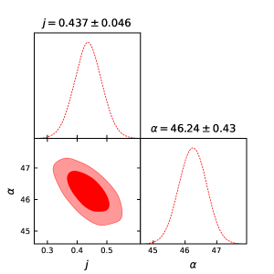
(a)

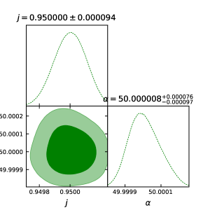
(b)

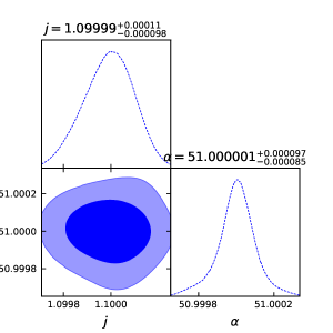
(c)

Figure 1: Figs. a, b, and c depict the likelihood contours for $H(z)$, $Pantheon$, and $H(z)+Pantheon$ dataset respectively corresponding to $1\sigma$ and $2\sigma$ confidence regions.

IV.3 Joint Datasets

To obtain the better constraint values of the model parameter, the joint dataset is used and the results are calculated by the $\chi_{HP}^{2}$ function, which is the sum of the functions $\chi_{Hub}^{2}$ and $\chi_{Pan}^{2}$ as

$$\chi_{HP}^{2}(j,\alpha)=\chi_{Hub}^{2}(j,\alpha)+\chi_{Pan}^{2}(j,\alpha).$$ (20)

The obtained values of $j$ and $\alpha$ from the above-mentioned observational datasets are placed in Table-1. According to the $\Lambda$CDM model, the present value of jerk parameter $j$ is $1$ and in our model, we obtained the best-fit value of $j$ which is close to 1 for the $Pantheon$ and joint datasets and for $H(z)$ dataset it is approximately $0.435$.

As the $\Lambda$CDM model is one of the standard models in cosmology and by comparing our model with the $\Lambda$CDM model we check the consistency of our model and for this purpose, error bar plots play a significant role. In our model, we have drawn the error bar plots for Hubble datasets and Type Ia Supernovae datasets. In Fig. 2(a) and Fig. 2(b), we observe the similarity between our model and the $\Lambda$CDM model with the error bar.

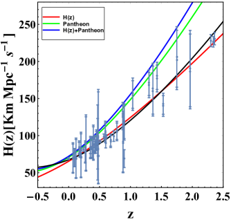
(a)

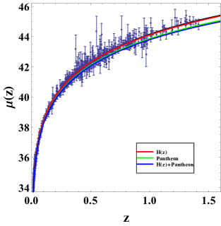
(b)

Figure 2: The error bar plots for $H(z)$ and Type Ia Supernovae datasets.

V Physical and Dynamical Components of the model

To explore the dynamical evolution of the universe, let us start with one of the essential parameters named as deceleration parameter ($q$). The deceleration parameter has been calculated in Eq. (5) and now we plot the curves for obtained best-fit values of $j$ and $\alpha$. For all three mentioned observational datasets, we perceive that $q$ is behaving alike i.e. in Fig. 3, at early times each trajectory is in the deceleration phase, and in late times as well as at present our model shows the accelerating phase of the universe. At present, the value of $q$ is $-0.25$ for $H(z)$, $Pantheon$, and joint datasets, and the value of redshift at the time of phase transition is $0.628$ for $H(z)$ dataset, $0.277$ for $Pantheon$ dataset and $0.239$ for $H(z)+Pantheon$ datasets which is clearly noticeable in the subplot of Fig. 3.

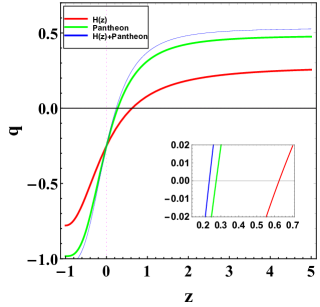
Figure 3: Plot of $q$  vs. $z$.

It is believed that after the Big Bang, the radiation-dominated era and matter-dominated era both are the major sections in the evolution of the Universe. The radiation-dominated era is required to anticipate primordial nucleosynthesis whereas in the matter-dominated era, element creation takes place. Therefore, keeping these points in mind we analyze the evolution of various physical parameters of our model.

For the fixed values of $\kappa=1$ and $\lambda=0.12$, the energy density and isotropic pressure have been plotted using Eqs. (14) and (15) in Fig. 4 for the obtained best-fit values of model parameters. Fig. 4(a) illustrates the evolution of energy density from high redshift to low redshift. As expected, the energy density decreases from early to late times for all datasets. In this model, the isotropic pressure is plotted in Fig. 4(b), which highlights that in the early universe, the value of pressure is highly positive and at present as well as in the future pressure is negative for all datasets. According to the standard cosmology, the negative pressure results expanding acceleration of the cosmos. The different value of EoS parameter ($\omega$) indicates the different forms of universe for example, $\omega=0$ $\to$ pressureless matter, $\omega\in(0,\frac{1}{3})$ $\to$ hot matter, $\omega=\frac{1}{3}$ $\to$ radiation, $\omega\in(\frac{1}{3},1)$ $\to$ hard universe, $\omega=1$ $\to$ stiff matter, $\omega>1$ $\to$ ekpyrotic matter, $\omega\in(0,-1)$ $\to$ quintessence universe, $\omega=-1$ $\to$ cosmological constant and $\omega<-1$ $\to$ Phantom universe. In our model, one can observe the different forms of the universe with respect to the changes in the value of $\omega$ (see Fig. 4(c)). Today and in the future, our model is a quintessence dark energy model.

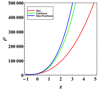
(a)

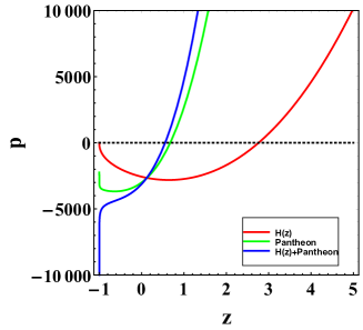
(b)

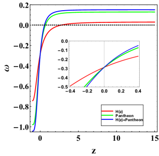
(c)

Figure 4: The graphs of $\rho$, $p$ and $\omega$  vs. $z$.

Besides phenomenal fields, there are some major points to explore such as the classification of singularities, casual structure, energy conditions, etc. In particular, energy conditions were originally formulated from the well-known Raychaudhuri equation. As it is valuable to explain the contribution of further geometrical terms in the stress-energy tensor such as effective pressure and effective energy density we study four energy conditions. The energy conditions are the diminution of time-like or null vector fields concerning the energy-momentum tensor and Einstein tensor obtained from Einstein field equations. Generally, four energy conditions are discussed in cosmological models namely, Weak energy condition (WEC), Null energy condition (NEC), Strong energy condition (SEC), and Dominant energy condition (DEC). These ECs are defined as: WEC: $\rho\geq 0,~{}\rho+p>0$, NEC: $\rho+p\geq 0$, SEC: $\rho+3p\geq 0$, and DEC: $\rho\geq|p|$.

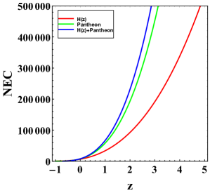
(a)

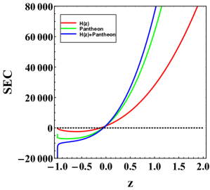
(b)

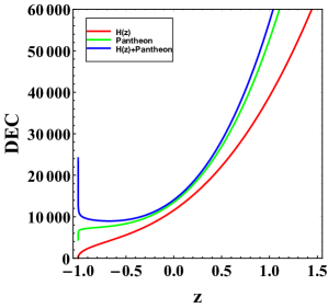
(c)

Figure 5: The plots for NEC, SEC, DEC.

In Fig. 5, we perceive that for all observational datasets NEC and DEC hold for the whole range of $z$, whereas SEC violates in the future.

VI Dynamical system stability

In this section, we employ the dynamical system technique to assess the stability of the system. To achieve this, we initially select a set of dimensionless variables as follows,

$$\Omega_{M}=\frac{\kappa\rho}{3H^{2}},\quad y=\frac{\kappa p}{H^{2}},\quad\delta=\kappa\lambda,$$ (21)

The variable $\Omega_{M}$ represents a time-dependent quantity, signifying the fractional energy density budget of the universe, while $y$ captures the dynamics of the corresponding pressure. We introduce a dimensionless constant, denoted as $\delta$, which can take any non-zero value. Utilizing Eq. (12) and Eq. (13), we express,

$$H^{2}=\frac{\kappa(3p\kappa\lambda-\rho+3\kappa\lambda\rho)}{-3+12\kappa\lambda},$$ (22)

and

$$\dot{H}=\frac{-\kappa}{2}(\rho+p).$$ (23)

Expressing Eq. (22) in terms of the dynamical variables that constrain $y$, we can represent this constraint in terms of $\Omega_{M}$ as,

$$y=\frac{-1+\Omega_{M}}{\delta}+4-3\Omega_{M}.$$ (24)

To analyze the dynamics of the system, we construct the autonomous system by calculating the first-order time derivative of the dynamical variable, as follows,

$$\Omega_{M}^{\prime}=\frac{d\Omega_{M}}{Hdt}=-(1-4\delta)(y+3\Omega_{M})-2\delta\left(j+\frac{3}{2}(y+3\Omega_{M})-1\right)+\Omega_{M}(y+3\Omega_{M}).$$ (25)

Here, $Hdt=dN=d\log a$. We have used $j=\frac{\dddot{a}}{aH^{3}}$ as a constant parameter. This constraint allows the evaluation of the system’s dynamics using a single parameter, resulting in a 1D phase space. The equation of state and deceleration parameter can then be expressed in terms of dynamical variables as,

$$\omega=\frac{p}{\rho}=\frac{y}{3\Omega_{M}},\quad q=-1+\frac{1}{2}(y+3\Omega_{M}).$$ (26)

We impose an additional constraint on the fractional energy density parameter, necessitating it to remain positive and bounded between $0$ and $1$,

$$0<\Omega_{M}\leq 1.$$ (27)

The critical points that satisfy this constraint are the only ones considered physically viable. The system produces two critical points, which are tabulated in Tab. 2. The qualitative behavior of these points is discussed in detail.

Table 2: The critical points and its nature.

Points	$\Omega_{M*}$	$\omega$	$d\Omega_{M}^{\prime}/d\Omega_{M}|_{\Omega_{M*}}$
$P_{1}$	$1-\frac{1}{2}\delta\left(\sqrt{8j+1}+5\right)$	Fig. LABEL:fig:eos_p1	$-\sqrt{8j+1}$
$P_{2}$	$\frac{1}{2}\delta\left(\sqrt{8j+1}-5\right)+1$	Fig. LABEL:fig:eos_p2	$\sqrt{8j+1}$

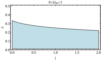
(a)

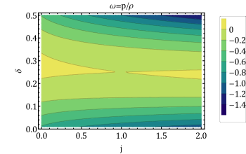
(b)

Figure 6: The plots for the constrained relation Eq. (27) and EoS $\omega$, in the parametric space of $(j,\delta)$ for the fixed point $P_{1}$.

• Point $P_{1}$: This critical point is dependent on both $j$ and $\delta$ and becomes a real point for $j>-1/8$. However, it cannot assume arbitrary values and must adhere to the constraint given by Eq. (27). The corresponding region of its existence has been plotted in Fig. LABEL:fig:x_existence_p1. The nature of the fixed point can be inferred from the equation of state $\omega$, as illustrated in Fig. LABEL:fig:eos_p1, further constraining the values of $j$ and $\delta$. The contour plot reveals that the point can exhibit both accelerating and non-accelerating solutions for $\delta<0.3$. However, for $\delta\geq 0.5$, the point yields a phantom solution; nevertheless, the fractional energy density violates the constraint relation. To assess the stability of the fixed point, we determined the first derivative $\frac{d\Omega_{M}^{\prime}}{d\Omega_{M}}\Big{|}_{\Omega_{M*}}$ at this point, resulting in a negative quantity. Following the stability discussion presented in Appendix A, we conclude that as $N\to+\infty$, the point becomes a stable fixed point corresponding to the future epoch of the universe. Conversely, at the past epoch, i.e., $N\to-\infty$, the point becomes unstable.

  

  (a)

  

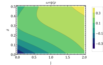
  (b)

  Figure 7: The plots for the constrained relation Eq. (27) and EoS parameter $\omega$, in the parametric space of $(j,\delta)$ for the fixed point $P_{2}$.

  

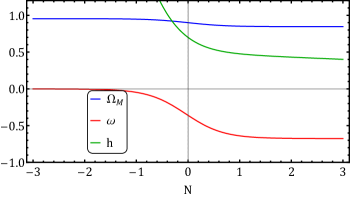
  (a)

  Figure 8: The evolution of cosmological parameters for $\delta=0.04,\ j=0.8$.

• Point $P_{2}$: The constraint of the point has been visualized in Fig. LABEL:fig:x_existence_p2, illustrating its existence for $j>-1/8$. The equation of state corresponding to this point is depicted in Fig. LABEL:fig:eos_p2, showing positive values and indicating non-accelerating characteristics. For $j>1.5$ and $\delta>0.4$, the point can mimic the radiation equation of state. However, within this range, the aforementioned point becomes unphysical. In the range $0.5<j<1.5$ and $0.01<\delta<0.2$, this point can exhibit characteristics of a pressure-less fluid. Upon evaluating stability, the derivative $\frac{d\Omega_{M}^{\prime}}{d\Omega_{M}}\Big{|}_{\Omega_{M*}}$ yields a positive value, indicating stability in the past epoch.

From the analysis of critical points and based on their characteristic properties, we have constrained $j$ and $\delta$. One of the critical points is found to be stable, producing an accelerating solution that represents the present epoch of the universe. To further analyze the system’s dynamics, we evaluate the evolution of cosmological parameters, i.e., $(\Omega_{M},\omega,h\equiv H/100)$ against $N=\log a$ in Fig. 8, spanning from the past epoch to the future epoch. We select benchmark points $(j=0.8,\delta=0.04)$ to ensure the existence of both fixed points simultaneously. In the past epoch, the fractional energy density dominates, and the corresponding equation of state is near $0$, indicating a matter-dominated phase of the universe. As the system evolves toward the present epoch, the equation of state increases towards negative values. In the future epoch, $\omega$ saturates to $-0.70$, and energy density saturates to $0.90$. Hence, the system exhibits quintessence-like behavior in the late-time epoch and produces matter characteristics in the past epoch of the universe. We have also depicted the evolution of the Hubble parameter $h(N)=H(N)/100$ using

$$\frac{dh}{dN}=-\frac{3}{2}h(N)\left(\frac{y}{3}+x\right).$$ (28)

The behavior indicates that in the past, the Hubble parameter increases, and as the system progresses into the future epoch, the Hubble parameter saturates to lower values.

VII Conclusion

In this work, we study Rastall’s theory of gravity, which is based on a variational principle. In this theory, we consider a non-minimal coupling between geometry and matter fields and discuss the recent theoretical developments in alternative theories of general relativity. This work is framed for the flat, isotropic, and homogeneous universe in the FLRW metric, where we have obtained the EFEs with the calculated value of the Hubble parameter in terms of the jerk parameter. Furthermore, we examine the essential physical and dynamical parameters one by one. We evaluate the best-fitted values of model parameters $\alpha$ and $j$ by the MCMC method, where we use the Hubble dataset, $Pantheon$ dataset, and their joint dataset.

The trajectories of the deceleration parameter for these best-fit values indicate the phase transition from deceleration to acceleration. At present, our model shows the accelerating universe.

Also, if we look at the behavior of energy density, it is monotonically decreased from high redshift to low redshift for all observational datasets. The isotropic pressure $p$ is positive in the early universe and holds a negative value at present as well as in the future, which indicates the presence of repulsive force and an accelerating expansion of the universe. According to the results of the EoS parameter, our model is a quintessence dark energy model at present. In Fig. 4, $\omega$ depicts the different dominating eras of the universe.

In this model, NEC and DEC both hold good but SEC violates which shows the existence of exotic matter in the universe. Hence, finally, we conclude that our model which is studied in Rastall gravity is a quintessence dark energy model.

Finally, we conducted a dynamical stability analysis of the system, treating the jerk parameter $j$ as a constant quantity, which imposes a vital constraint on the system. Our findings revealed a 1D phase space, with the system yielding two critical points. One critical point results in a stable accelerating solution in the future epoch, resembling the behavior of a quintessential dark energy model. The other critical point exhibits non-accelerating characteristics, similar to dark matter fluid, and stabilizes at the past epoch. Thus, the qualitative behavior of the system demonstrates that Rastall’s theory of gravity can consistently account for different phases, namely the matter-dominated and accelerating epochs of the universe.

Acknowledgements

J. K. Singh wishes to thank Joao Luis Rosa, Institute of Physics, University of Tartu, W. Ostwaldi 1, 50411 Tartu, Estonia for fruitful discussions.

Data Availability Statement No new data were created or analyzed in this study.

Appendix A Dynamical system in 1D

Consider the autonomous equation in 1D is:

$$\dfrac{dx}{dN}=\dot{x}=f(x).$$ (29)

Suppose $x_{0}\in\mathbb{R}^{n}$ is a fixed point of the autonomous equation such that $f(x_{0})=0$. To determine the stability of the system at this fixed point, we perturb the system around it as,

$$x=x_{0}+\epsilon,$$ (30)

where, $\epsilon\ll 1$. We expand $f(x)$ using Taylor’s series around the fixed point $x_{0}$ as,

$$f(x)=f(x_{0})+\dfrac{df}{dx}\Big{|}_{x_{0}}(x-x_{0})+......$$ (31)

Inserting it into the autonomous equation Eq. (29) and truncating the series after the first order, we obtain,

$$\begin{split}\dot{\epsilon}&=f^{\prime}(x_{0})\epsilon,\\ \implies\epsilon&=C\exp(f^{\prime}(x_{0})\,N).\end{split}$$ (32)

Here, $C$ is an integration constant. Observing Eq. (32), as $N\rightarrow+\infty$, the perturbation increases (decreases) when $f^{\prime}(x_{0})>0\ (<0)$, indicating the system becomes unstable (stable) at that point.

References

- [1] J. K. Singh, A. Singh, G. K. Goswami and J. Jena, Annals Phys. 443, 168958 (2022).
- [2] J. K. Singh, Shaily, A. Singh, A. Beesham and H. Shabani, Annals Phys. 455, 169382 (2023).
- [3] J. K. Singh, H. Balhara, K. Bamba and J. Jena, JHEP 03, 191 (2023) [erratum: JHEP 04, 049 (2023)].
- [4] J. K. Singh, K. Bamba, R. Nagpal and S. K. J. Pacif, Phys. Rev. D 97, 123536 (2018).
- [5] J. K. Singh, Shaily and K. Bamba, Chin. J. Phys. 84, 371-380 (2023).
- [6] J. K. Singh and R. Nagpal, Eur. Phys. J. C 80, no.4, 295 (2020).
- [7] J. K. Singh, A. Singh, Shaily and J. Jena, Chin. J. Phys. 86, 616-627 (2023).
- [8] R. Nagpal, S. K. J. Pacif, J. K. Singh, K. Bamba and A. Beesham, Eur. Phys. J. C 78, no.11, 946 (2018).
- [9] P. Rastall, Phys. Rev. D 6, 3357-3359 (1972).
- [10] L. Lindblom, W. A. Hiscock, J. Phys. A: Math. Gen. 15, 1827-1830 (1982).
- [11] M. Visser, Phys. Lett. B 782, 83-86 (2018).
- [12] F. Darabi, H. Moradpour, I. Licata, Y. Heydarzade and C. Corda, Eur. Phys. J. C 78, 25 (2018).
- [13] S. Santos Da Costa, F. V. Roig, J. S. Alcaniz, S. Capozziello, M. De Laurentis and M. Benetti, Class. Quant. Grav. 35, no.7, 075013 (2018).
- [14] G. J. Olmo, Phys. Rev. D 72, 083505 (2005).
- [15] L. K. Duchaniya, S. V. Lohakare, B. Mishra and S. K. Tripathy, Eur. Phys. J. C 82, no.5, 448 (2022).
- [16] G. Kofinas, G. Leon and E. N. Saridakis, Class. Quant. Grav. 31, 175011 (2014).
- [17] S. A. Kadam, B. Mishra and J. Said Levi, Eur. Phys. J. C 82, no.8, 680 (2022).
- [18] S. A. Kadam, N. P. Thakkar and B. Mishra, Eur. Phys. J. C 83, no.9, 809 (2023).
- [19] A. Stachowski and M. Szydłowski, Eur. Phys. J. C 76, no.11, 606 (2016).
- [20] N. Roy and N. Banerjee, Phys. Rev. D 95, no.6, 064048 (2017).
- [21] W. Khyllep, J. Dutta, E. N. Saridakis and K. Yesmakhanova, Phys. Rev. D 107, no.4, 044022 (2023).
- [22] W. Khyllep, J. Dutta, S. Basilakos and E. N. Saridakis, Phys. Rev. D 105, no.4, 043511 (2022).
- [23] R. G. Landim, Eur. Phys. J. C 79, no.11, 889 (2019).
- [24] A. Alho, C. Uggla and J. Wainwright, JCAP 09, 045 (2019).
- [25] A. Singh, G. P. Singh and A. Pradhan, Int. J. Mod. Phys. A 37, no.16, 2250104 (2022).
- [26] N. Roy and N. Banerjee, Annals Phys. 356, 452-466 (2015).
- [27] S. Das, S. Hussain, D. Nandi, R. O. Ramos and R. Silva, Phys. Rev. D 108, no.8, 083517 (2023).
- [28] S. Chakraborty, K. Bamba and A. Saa, Phys. Rev. D 99, no.6, 064048 (2019).
- [29] S. D. Odintsov and V. K. Oikonomou, Phys. Rev. D 96, no.10, 104049 (2017).
- [30] A. Alho, S. Carloni and C. Uggla, JCAP 08, 064 (2016).
- [31] S. Carloni, JCAP 09, 013 (2015).
- [32] S. D. Odintsov and V. K. Oikonomou, Phys. Rev. D 98, no.2, 024013 (2018).
- [33] V. K. Oikonomou and N. Chatzarakis, Nucl. Phys. B 956, 115023 (2020).
- [34] N. Roy and N. Banerjee, [arXiv:1412.0837 [gr-qc]].
- [35] S. Bahamonde, C. G. Böhmer, S. Carloni, E. J. Copeland, W. Fang and N. Tamanini, Phys. Rept. 775-777, 1-122 (2018).
- [36] H. Shabani and A. H. Ziaie, Eur. Phys. J. C 77, no.5, 282 (2017).
- [37] H. Shabani, A. De, T. H. Loo and E. N. Saridakis, [arXiv:2306.13324 [gr-qc]].
- [38] H. Shabani, A. De and T. H. Loo, Eur. Phys. J. C 83, no.6, 535 (2023).
- [39] V. K. Oikonomou, Int. J. Mod. Phys. D 27, no.05, 1850059 (2018).
- [40] N. Chatzarakis and V. K. Oikonomou, Annals Phys. 419, 168216 (2020).
- [41] L. K. Duchaniya, K. Gandhi and B. Mishra, [arXiv:2303.09076 [gr-qc]].
- [42] S. V. Lohakare, K. Rathore and B. Mishra, Class. Quant. Grav. 40, no.21, 215009 (2023).
- [43] S. A. Kadam, S. V. Lohakare and B. Mishra, Annals Phys. 460, 169563 (2024).
- [44] L. Pati, S. A. Narawade, S. K. Tripathy and B. Mishra, Eur. Phys. J. C 83, no.5, 445 (2023).
- [45] S. A. Narawade, M. Koussour and B. Mishra, Nucl. Phys. B 992, 116233 (2023).
- [46] R. Bhagat, S. A. Narawade, B. Mishra and S. K. Tripathy, Phys. Dark Univ. 42, 101358 (2023).
- [47] J. De-Santiago, J. L. Cervantes-Cota and D. Wands, Phys. Rev. D 87, no.2, 023502 (2013).
- [48] J. Dutta, W. Khyllep and H. Zonunmawia, Eur. Phys. J. C 79, no.4, 359 (2019).
- [49] S. Carloni, F. S. N. Lobo, G. Otalora and E. N. Saridakis, Phys. Rev. D 93, 024034 (2016).
- [50] C. G. Boehmer, N. Tamanini and M. Wright, Phys. Rev. D 91, no.12, 123003 (2015).
- [51] A. Chatterjee, S. Hussain and K. Bhattacharya, Phys. Rev. D 104, no.10, 2021 (2021).
- [52] S. Hussain, A. Chatterjee and K. Bhattacharya, Phys. Rev. D 108, no.10, 103502 (2023).
- [53] B. Mirza and F. Oboudiat, Int. J. Geom. Meth. Mod. Phys. 13, no.09, 1650108 (2016).
- [54] H. Shabani, A. H. Ziaie and H. Moradpour, Annals Phys. 444, 169058 (2022).
- [55] G. F. Silva, O. F. Piattella, J. C. Fabris, L. Casarini and T. O. Barbosa, Grav. Cosmol. 19, 156-162 (2013).
- [56] A. Singh, R. Raushan and R. Chaubey, Can. J. Phys. 99, no.12, 1073-1081 (2021).
- [57] H. Shabani, H. Moradpour and A. H. Ziaie, Phys. Dark Univ. 36, 101047 (2022).
- [58] W. Khyllep and J. Dutta, Phys. Lett. B 797, 134796 (2019).
- [59] S. Ghosh, S. Dey, A. Das, A. Chanda and B. C. Paul, JCAP 07, 004 (2021).
- [60] M. F. A. R. Sakti, A. Suroso and F. P. Zen, Annals Phys. 413, 168062 (2020).
- [61] M. F. A. R. Sakti, A. Suroso, A. Sulaksono and F. P. Zen, Phys. Dark Univ. 35, 100974 (2022).
- [62] S. Guo, K. J. He, G. R. Li and G. P. Li, Class. Quant. Grav. 38, no.16, 165013 (2021).
- [63] G. G. L. Nashed, Universe 8, no.10, 510 (2022).
- [64] D. J. Gogoi and U. D. Goswami, Phys. Dark Univ. 33, 100860 (2021).
- [65] C. Y. Shao, Y. J. Tan, C. G. Shao, K. Lin and W. L. Qian, Chin. Phys. C 46, no.10, 105103 (2022).
- [66] B. Narzilloev, I. Hussain, A. Abdujabbarov and B. Ahmedov, Eur. Phys. J. Plus 137, no.5, 645 (2022).
- [67] Y. Heydarzade, H. Moradpour and F. Darabi, Can. J. Phys. 95, no.12, 1253-1256 (2017).
- [68] A. Singh and K. C. Mishra, Eur. Phys. J. Plus 135, no.9, 752 (2020).
- [69] A. Singh and A. Pradhan, Indian J. Phys. 97, no.2, 631-641 (2023).
- [70] Chlouverakis, E. Konstantinos and J. C. Sprott, Chaos, Solitons & Fractals. 28, no.3, 739–746 (2006).
- [71] A. Al Mamon and K. Bamba, Eur. Phys. J. C 78, no.10, 862 (2018).
- [72] N. Myrzakulov, M. Koussour, A. H. A. Alfedeel and H. M. Elkhair, Chin. J. Phys. 86, 300-312 (2023).
- [73] L. Chimento and M. I. Forte, Phys. Lett. B 666, 205-211 (2008).
- [74] J. K. Singh, Shaily, S. Ram, J. R. L. Santos and J. A. S. Fortunato, Int. J. Mod. Phys. D 32, 2350040 (2023).
- [75] Shaily, A. Singh, J. K. Singh and S. Ray, [arXiv:2402.01780 [gr-qc]].
- [76] J. K. Singh, Shaily, H. Balhara, K. Bamba and J. Jena, Astron. Comput. 46 (2024), 100790.
- [77] J. K. Singh, H. Balhara, Shaily and P. Singh, Astron. Comput. 46 (2024), 100795.
- [78] H. Balhara, J. K. Singh and E. N. Saridakis, [arXiv:2312.17277 [gr-qc]].
- [79] Shaily, M. Zeyauddin and J. K. Singh, arXiv:220.05076 [gr-qc].
- [80] D. M. Scolnic et al. [Pan-STARRS1], Astrophys. J. 859, no.2, 101 (2018).
- [81] A. G. Riess, R. P. Kirshner, B. P. Schmidt, S. Jha, P. Challis, P. M. Garnavich, A. A. Esin, C. Carpenter, R. Grashius and R. E. Schild, et al. Astron. J. 117, 707-724 (1999).
- [82] S. Jha, R. P. Kirshner, P. Challis, P. M. Garnavich, T. Matheson, A. M. Soderberg, G. J. M. Graves, M. Hicken, J. F. Alves and H. G. Arce, et al. Astron. J. 131, 527-554 (2006).
- [83] M. Hicken, P. Challis, S. Jha, R. P. Kirsher, T. Matheson, M. Modjaz, A. Rest and W. M. Wood-Vasey, Astrophys. J. 700, 331-357 (2009).
- [84] C. Contreras, M. Hamuy, M. M. Phillips, G. Folatelli, N. B. Suntzeff, S. E. Persson, M. Stritzinger, L. Boldt, S. Gonzalez and W. Krzeminski, et al. Astron. J. 139, 519-539 (2010).
- [85] M. Sako et al. [SDSS], Publ. Astron. Soc. Pac. 130, no.988, 064002 (2018).