Model Assessment and Selection under Temporal Distribution Shift

Abstract

We investigate model assessment and selection in a changing environment, by synthesizing datasets from both the current time period and historical epochs. To tackle unknown and potentially arbitrary temporal distribution shift, we develop an adaptive rolling window approach to estimate the generalization error of a given model. This strategy also facilitates the comparison between any two candidate models by estimating the difference of their generalization errors. We further integrate pairwise comparisons into a single-elimination tournament, achieving near-optimal model selection from a collection of candidates. Theoretical analyses and numerical experiments demonstrate the adaptivity of our proposed methods to the non-stationarity in data.

Keywords: Model assessment, model selection, temporal distribution shift, adaptivity.

1 Introduction

Statistical learning theory is traditionally founded on the assumption of a static data distribution, where statistical models are trained and deployed in the same environment. However, this assumption is often violated in practice, where the data distribution keeps changing over time. The temporal distribution shift can lead to serious decline in model performance post-deployment, which underlines the critical need to monitor models and detect potential degradation.

Moreover, one often needs to choose among multiple candidate models originating from different learning algorithms (e.g., linear regression, random forests, neural networks) and hyperparameters (e.g., penalty parameter, step size, time window for training). Temporal distribution shift poses a major challenge to model selection, as past performance may not reliably predict future outcomes. Learners usually have to work with limited data from the current time period and abundant historical data, whose distributions may vary significantly.

Main contributions.

In this paper, we develop principled approaches to model assessment and selection under unknown temporal distribution shift.

• (Model assessment) We propose an adaptive window method for estimating a model’s generalization error by selectively utilizing historical data.

• (Model selection) The above method can be used to compare any pair of models when applied to the difference between their generalization errors. Based on this, we develop a single-elimination tournament scheme for selecting the best model from a pool of candidates.

Furthermore, we provide theoretical guarantees and numerical results to demonstrate the adaptivity of our methods to non-stationarity.

Related works.

Model assessment and selection are fundamental pillars in statistical learning (Hastie et al., 2009). Hold-out and cross-validation are arguably the most popular methods in practice. However, in the presence of distribution shift, the validation data may no longer accurately represent the test cases. This challenge has attracted considerable attention over the past two decades (Quinonero-Candela et al., 2022). Existing works mostly focused on the static scenario where the validation data comprises independent samples from a fixed distribution. These methods do not apply when the environment is continuously changing over time. Rolling windows offer a practical solution to this issue and have been widely adopted for learning under temporal changes (Bifet and Gavalda, 2007; Hanneke et al., 2015; Mohri and Muñoz Medina, 2012; Mazzetto and Upfal, 2023; Mazzetto et al., 2023; Huang and Wang, 2023). Our method automatically selects a window tailored to the underlying non-stationarity near a given time. The strategy is inspired by the Goldenshluger-Lepski method for bandwidth selection in non-parametric estimation (Goldenshluger and Lepski, 2008).

Adaptation to a non-stationary environment has emerged as a prominent area of study in online learning, where the goal is to attain a small cumulative error over an extended time horizon (Hazan and Seshadhri, 2009; Besbes et al., 2015; Daniely et al., 2015; Jadbabaie et al., 2015; Wei and Luo, 2021; Gibbs and Candes, 2021; Bai et al., 2022). A classical problem in this area is prediction from expert advice (Littlestone and Warmuth, 1994), which aims to track the best expert in the long run. In contrast, our approach focuses on evaluating a model or selecting from multiple candidates at a specific point in time, leveraging offline data collected from the past. Its performance is measured over the current data distribution. Consequently, our problem can be viewed as one of transfer learning, with source data from historical epochs and target data from the current distribution. We point out that our algorithms for the offline setting can be used as a sub-routine for online model selection, where the candidate models may vary across different time points.

Our problem also is different from change-point detection (Niu et al., 2016; Truong et al., 2020). The latter typically assumes that distribution shifts occur only at a small number of times called change points. Our setting allows changes to happen at every time period with arbitrary magnitudes, encompassing a much broader spectrum of shift patterns.

Notation.

Let $\mathbb{Z}_{+}=\{1,2,...\}$ be the set of positive integers. For $n\in\mathbb{Z}_{+}$, let $[n]=\{1,2,...,n\}$. For $x\in\mathbb{R}$, define $x_{+}=\max\{x,0\}$. For $a,b\in\mathbb{R}$, define $a\wedge b=\min\{a,b\}$. For non-negative sequences $\{a_{n}\}_{n=1}^{\infty}$ and $\{b_{n}\}_{n=1}^{\infty}$, we write $a_{n}=\mathcal{O}(b_{n})$ if there exists $C>0$ such that for all $n\in\mathbb{Z}_{+}$, $a_{n}\leq Cb_{n}$. Unless otherwise stated, $a_{n}\lesssim b_{n}$ also represents $a_{n}=\mathcal{O}(b_{n})$. We write $a_{n}=o(b_{n})$ if $a_{n}/b_{n}\to 0$ as $n\to\infty$.

2 Problem setup

Let $\mathcal{Z}$ and $\mathcal{F}$ be spaces of samples and models, respectively. Denote by $\ell:~{}\mathcal{F}\times\mathcal{Z}$ a loss function. The quantity $\ell(f,z)$ measures the loss incurred by a model $f\in\mathcal{F}$ on a sample $z\in\mathcal{Z}$. At time $t\in\mathbb{Z}_{+}$, the quality of a model $f$ is measured by its generalization error (also called risk or population loss) $L_{t}(f)=\mathbb{E}_{z\sim\mathcal{P}_{t}}\ell(f,z)$ over the current data distribution $\mathcal{P}_{t}$. When the environment changes over time, the distributions $\{\mathcal{P}_{t}\}_{t=1}^{\infty}$ can be different.

Suppose that at each time $t$, we receive a batch of $B_{t}\in\mathbb{Z}_{+}$ i.i.d. samples $\mathcal{B}_{t}=\{z_{t,i}\}_{i=1}^{B_{t}}$ from $\mathcal{P}_{t}$, independent of the history. We seek to solve the following two questions based on the data $\{\mathcal{B}_{j}\}_{j=1}^{t}$:

Problem 2.1 (Model assessment).

Given a model $f\in\mathcal{F}$, how to estimate its population loss $L_{t}(f)$?

Problem 2.2 (Model selection).

Given a collection of candidate models $\{f_{r}\}_{r=1}^{m}\subseteq\mathcal{F}$, how to select one with a small population loss? In other words, we want to choose $\widehat{r}\in[m]$ so that $L_{t}(f_{\widehat{r}})\approx\min_{r\in[m]}L_{t}(f_{r})$.

3 Model Assessment

In this section we study Problem 2.1, under the assumption that the loss $\ell$ is bounded.

Assumption 3.1 (Bounded loss).

The loss function $\ell$ takes values in a given interval $[a,b]$.

In fact, we will consider a more general problem.

Problem 3.1 (Mean estimation).

Let $\{\mathcal{Q}_{j}\}_{j=1}^{t}$ be probability distributions over $[a,b]$ and $\{\mathcal{D}_{j}\}_{j=1}^{t}$ be independent datasets, where $\mathcal{D}_{j}=\{u_{j,i}\}_{i=1}^{B_{j}}$ consists of $B_{j}$ i.i.d. samples from $\mathcal{Q}_{j}$. Given $\{\mathcal{D}_{j}\}_{j=1}^{t}$, how to estimate the mean $\mu_{t}$ of $\mathcal{Q}_{t}$?

Problem 2.1 is a special case of Problem 3.1 with $u_{j,i}=\ell(f,z_{j,i})$ and $\mu_{t}=L_{t}(f)$. To tackle Problem 3.1, a natural idea is to take a look-back window $k\in[t]$, and approximate $\mu_{t}$ by the sample average over the $k$ most recent periods:

$$\widehat{\mu}_{t,k}=\bigg{(}\sum_{j=t-k+1}^{t}B_{j}\bigg{)}^{-1}\sum_{j=t-k+1}^{t}\sum_{i=1}^{B_{j}}u_{j,i}.$$ (3.1)

To measure the quality of $\widehat{\mu}_{t,k}$, we invoke the Bernstein inequality (Boucheron et al., 2013). See Section A.1 for the proof of the version we use.

Lemma 3.1 (Bernstein bound).

Let $\{x_{i}\}_{i=1}^{n}$ be independent random variables taking values in $[a,b]$ almost surely. Define the average variance $\sigma^{2}=\frac{1}{n}\sum_{i=1}^{n}\operatorname{{\rm var}}(x_{i})$. For any $\delta\in(0,1)$, with probability at least $1-\delta$,

$$\bigg{|}\frac{1}{n}\sum_{i=1}^{n}(x_{i}-\mathbb{E}x_{i})\bigg{|}\leq\sigma\sqrt{\frac{2\log(2/\delta)}{n}}+\frac{2(b-a)\log(2/\delta)}{3n}.$$

Denote by $\mu_{j}$ and $\sigma_{j}^{2}$ the mean and the variance of $\mathcal{Q}_{j}$, respectively. Let $B_{t,k}=\sum_{j=t-k+1}^{t}B_{j}$,

$$\mu_{t,k}=\frac{1}{B_{t,k}}\sum_{j=t-k+1}^{t}B_{j}\mu_{j},\qquad\sigma_{t,k}^{2}=\frac{1}{B_{t,k}}\sum_{j=t-k+1}^{t}B_{j}\sigma_{j}^{2}.$$

From Lemma 3.1 and the triangle inequality

$$|\widehat{\mu}_{t,k}-\mu_{t}|\leq|\widehat{\mu}_{t,k}-\mu_{t,k}|+|\mu_{t,k}-\mu_{t}|,$$

we obtain the following bias-variance decomposition of the approximation error of $\widehat{\mu}_{t,k}$.

Corollary 3.1.

For $t\in\mathbb{Z}_{+}$, $k\in[t]$ and $\delta\in(0,1)$, define $M=b-a$,

$$\phi(t,k)=\max_{t-k+1\leq j\leq t}|\mu_{j}-\mu_{t}|,$$

$$\psi(t,k,\delta)=\begin{cases}M,&\ \text{if }B_{t,k}=1\\[4.0pt] \sigma_{t,k}\sqrt{\frac{2\log(2/\delta)}{B_{t,k}}}+\frac{2M\log(2/\delta)}{3B_{t,k}},&\ \text{if }B_{t,k}\geq 2\end{cases}.$$

With probability at least $1-\delta$,

$$|\widehat{\mu}_{t,k}-\mu_{t}|\leq\phi(t,k)+\psi(t,k,\delta).$$

Here $\phi(t,k)$ upper bounds the bias induced by using data from the $k$ most recent periods, and $\psi(t,k,\delta)$ upper bounds the stochastic error associated with $\widehat{\mu}_{t,k}$. We seek an answer to the following question:

How to find $\widehat{k}$ such that $|\widehat{\mu}_{t,\widehat{k}}-\mu_{t}|$ is comparable to $\min_{k\in[t]}\{\phi(t,k)+\psi(t,k,\delta)\}$?

Both $\phi$ and $\psi$ involve unknown quantities $\mu_{j}$ and $\sigma_{j}$, so direct minimization over $k\in[t]$ is infeasible. In the following, we will construct proxies for $\psi$ and $\phi$ that are computable from data.

We first work on $\psi(t,k,\delta)$. A natural approximation of $\sigma_{t,k}^{2}$ is the sample variance over the $k$ most recent periods, given by

$$\widehat{v}_{t,k}^{2}=\frac{1}{B_{t,k}-1}\sum_{j=t-k+1}^{t}\sum_{i=1}^{B_{j}}(u_{j,i}-\widehat{\mu}_{t,k})^{2}.$$ (3.2)

It has been used for deriving empirical versions of the Bernstein inequality (Audibert et al., 2007; Maurer and Pontil, 2009). Based on the estimate $\widehat{v}_{t,k}^{2}$, we define our proxy as

$$\widehat{\psi}(t,k,\delta)=\begin{cases}M,&\ \text{if }B_{t,k}=1\\[4.0pt] \widehat{v}_{t,k}\sqrt{\frac{2\log(2/\delta)}{B_{t,k}}}+\frac{8M\log(2/\delta)}{3(B_{t,k}-1)},&\ \text{if }B_{t,k}\geq 2\end{cases}.$$ (3.3)

As Lemma 3.2 shows, with high probability, $\widehat{\psi}$ is an upper bound on $\psi$, and is at the same time not too much larger than $\psi$. Its proof is deferred to Section A.2.

Lemma 3.2.

Choose any $\delta\in(0,1)$. If $B_{t,k}\geq 2$, define

$$\xi(t,k,\delta)=\sqrt{\frac{4\log(2/\delta)}{B_{t,k}}}\max_{t-k+1\leq j\leq t}|\mu_{j}-\mu_{t}|+\frac{13(b-a)\log(2/\delta)}{3(B_{t,k}-1)}.$$

If $B_{t,k}=1$, define $\xi(t,k,\delta)=0$. Then

$$\mathbb{P}\left(\psi(t,k,\delta)\leq\widehat{\psi}(t,k,\delta)\right)\geq 1-\delta$$

$$\mathbb{P}\left(\widehat{\psi}(t,k,\delta)\leq\psi(t,k,\delta)+\xi(t,k,\delta)\right)\geq 1-\delta.$$

Combining Corollary 3.1 with the first bound in Lemma 3.2 immediately gives the following useful corollary.

Corollary 3.2.

Let $\delta\in(0,1)$. With probability at least $1-2t\delta$, it holds

$$|\widehat{\mu}_{t,k}-\mu_{t}|\leq\phi(t,k)+\widehat{\psi}(t,k,\delta),\quad\forall k\in[t].$$ (3.4)

To construct a proxy for $\phi(t,k)$, we borrow ideas from the Goldenshluger-Lepski method for adaptive non-parametric estimation (Goldenshluger and Lepski, 2008). Define

$$\widehat{\phi}(t,k,\delta)=\max_{i\in[k]}\bigg{(}|\widehat{\mu}_{t,k}-\widehat{\mu}_{t,i}|-[\widehat{\psi}\left(t,k,\delta\right)+\widehat{\psi}\left(t,i,\delta\right)]\bigg{)}_{+}.$$ (3.5)

We now give an interpretation of $\widehat{\phi}$. In light of the bias-variance decomposition in Corollary 3.1, the quantity

$$|\widehat{\mu}_{t,k}-\widehat{\mu}_{t,i}|-[\widehat{\psi}\left(t,k,\delta\right)+\widehat{\psi}\left(t,i,\delta\right)]$$ (3.6)

can be viewed as a measure of the bias between the windows $k$ and $i$, where subtracting $\widehat{\psi}\left(t,k,\delta\right)$ and $\widehat{\psi}\left(t,i,\delta\right)$ eliminates the stochastic error and teases out the bias. Indeed, as the following lemma shows, $\widehat{\phi}(t,k,\delta)\leq 2\phi(t,k)$ holds with high probability. Its proof is given in Section A.3.

Lemma 3.3.

When the event (3.4) happens,

$$0\leq\widehat{\phi}(t,k,\delta)\leq 2\phi(t,k).$$

We take the positive part in (3.5) so that when the quantity (3.6) is negative, we regard the bias as dominated by the stochastic error and hence negligible. Taking maximum over all windows $i\in[k]$ makes sure that we detect all possible biases between window $k$ and the smaller windows.

Replacing $\psi$ and $\phi$ with their proxies $\widehat{\psi}$ and $\widehat{\phi}$ gives Algorithm 1. We note that the quantities $\widehat{\mu}_{t,k}$ and $\widehat{v}_{t,k}$ can be conveniently computed from summary statistics of individual datasets. Define empirical first and second moments in the $j$-th time period, $\widehat{\mu}_{j}=B_{j}^{-1}\sum_{i=1}^{B_{j}}u_{j,i}$ and $\widehat{\omega}_{j}=B_{j}^{-1}\sum_{i=1}^{B_{j}}u_{j,i}^{2}$. Then,

$$\widehat{\mu}_{t,k}=\frac{1}{B_{t,k}}\sum_{j=t-k+1}^{t}B_{j}\widehat{\mu}_{j},$$ (3.7)

$$\widehat{v}_{t,k}^{2}=\frac{B_{t,k}}{B_{t,k}-1}\cdot\bigg{(}\frac{1}{B_{t,k}}\sum_{j=t-k+1}^{t}B_{j}\widehat{\omega}_{j}-\widehat{\mu}_{t,k}^{2}\bigg{)}.$$ (3.8)

  Input: Data $\{\mathcal{D}_{j}\}_{j=1}^{t}$, hyperparameters $\delta$ and $M$.

  for $k=1,\cdots,t$ do

     Compute $\widehat{\mu}_{t,k}$, $\widehat{v}_{t,k}$, $\widehat{\psi}(t,k,\delta)$ and $\widehat{\phi}(t,k,\delta)$ according to (3.1), (3.2), (3.3) and (3.5).

  end for

  Choose any $\widehat{k}\in\mathop{\mathrm{argmin}}_{k\in[t]}\{\widehat{\phi}(t,k,\delta)+\widehat{\psi}(t,k,\delta)\}$.

  Output: $\widehat{\mu}_{t,\widehat{k}}$.

Algorithm 1 Adaptive Rolling Window for Mean Estimation (Problem 3.1)

We now present theoretical guarantees for Algorithm 1.

Theorem 3.1.

Let Assumption 3.1 hold. Choose $\delta\in(0,1)$. With probability at least $1-3t\delta$, the output of Algorithm 1 satisfies

$$|\widehat{\mu}_{t,\widehat{k}}-\mu_{t}|\lesssim\min_{k\in[t]}\{\phi(t,k)+\psi(t,k,\delta)\}.$$

Here $\lesssim$ only hides a logarithmic factor of $\delta^{-1}$.

Theorem 3.1 states that the selected window $\widehat{k}$ is near-optimal for the error bound in Corollary 3.1 derived from bias-variance decomposition. Before proving the theorem, let us use a toy example to illustrate this oracle property. Imagine that the environment remained unchanged over the past $K$ time periods but had been different before, i.e. $\mathcal{P}_{t-K}\neq\mathcal{P}_{t-K+1}=\cdots=\mathcal{P}_{t}$. If $K$ were known, one could take the window size $K$ and output $\widehat{\mu}_{t,K}$ as an estimate of $\mu_{t}$. Theorem 3.1 implies that $\widehat{\mu}_{t,\widehat{k}}$ is at least comparable to $\widehat{\mu}_{t,K}$ in terms of the estimation error. Therefore, Algorithm 1 automatically adapts to the local stationarity and is comparable to using $B_{t,K}$ i.i.d. samples. Up to logarithmic factors, we have a Bernstein-type bound

$$|\widehat{\mu}_{t,\widehat{k}}-\mu_{t}|\lesssim\frac{\sigma_{t}}{\sqrt{B_{t,K}}}+\frac{1}{B_{t,K}}.$$

We now turn to the proof of Theorem 3.1. A key ingredient is the following lemma, which can be seen as an empirical version of Theorem 3.1 with $\psi$ replaced by $\widehat{\psi}$.

Lemma 3.4.

Let the event (3.4) happen, which has probability at least $1-2t\delta$. Then the window $\widehat{k}$ satisfies

$$|\widehat{\mu}_{t,\widehat{k}}-\mu_{t}|\leq 3\min_{k\in[t]}\{\phi(t,k)+\widehat{\psi}(t,k,\delta)\}.$$

Proof.

For any $k\in[\widehat{k}]$,

$$|\widehat{\mu}_{t,\widehat{k}}-\mu_{t}|\leq|\widehat{\mu}_{t,\widehat{k}}-\widehat{\mu}_{t,k}|+|\widehat{\mu}_{t,k}-\mu_{t}|$$

$$\leq\left[\widehat{\phi}(t,\widehat{k},\delta)+\widehat{\psi}(t,\widehat{k},\delta)+\widehat{\psi}(t,k,\delta)\right]+\left[\phi(t,k)+\widehat{\psi}(t,k,\delta)\right]$$ (by (3.5) and (3.4) )

$$=\left[\widehat{\phi}(t,\widehat{k},\delta)+\widehat{\psi}(t,\widehat{k},\delta)\right]+\left[\phi(t,k)+2\widehat{\psi}(t,k,\delta)\right]$$

$$\leq\left[\widehat{\phi}(t,k,\delta)+\widehat{\psi}(t,k,\delta)\right]+\left[\phi(t,k)+2\widehat{\psi}(t,k,\delta)\right] \widehat{k}$$ (by the definition of )

$$\leq\left[2\phi(t,k)+\widehat{\psi}(t,k,\delta)\right]+\left[\phi(t,k)+2\widehat{\psi}(t,k,\delta)\right]$$ (by Lemma 3.3)

$$=3\left[\phi(t,k)+\widehat{\psi}(t,k,\delta)\right].$$

On the other hand, for any $k\in\{\widehat{k}+1,\cdots,t\}$,

$$|\widehat{\mu}_{t,\widehat{k}}-\mu_{t}|\leq\phi(t,\widehat{k})+\widehat{\psi}(t,\widehat{k},\delta)$$ (by (3.4))

$$\leq\phi(t,k)+\left[\widehat{\psi}(t,\widehat{k},\delta)+\widehat{\phi}(t,\widehat{k},\delta)\right]$$ (by Lemma 3.3)

$$\leq\phi(t,k)+\left[\widehat{\psi}(t,k,\delta)+\widehat{\phi}(t,k,\delta)\right] \widehat{k}$$ (by the definition of )

$$\leq 3\left[\phi(t,k)+\widehat{\psi}(t,k,\delta)\right].$$ (by Lemma 3.3)

The proof is finished by taking minimum over $k\in[t]$. ∎

Combining Lemma 3.4 and the second bound in Lemma 3.2 proves Theorem 3.1. We provide a full proof in Section A.4, along with a more precise bound.

4 Model Selection

In this section, we consider Problem 2.2. We will first study the case of selection between two models, and then extend the approach to the general case of $m\in\mathbb{Z}_{+}$ models.

4.1 Warmup: Model Comparison

We first consider the case $m=2$, where the goal is to compare two models $f_{1}$ and $f_{2}$, and choose the better one. As in Section 3, using a look-back window $k\in[t]$, we can estimate $L_{t}(f)$ by

$$\widehat{L}_{t,k}(f)=\frac{1}{B_{t,k}}\sum_{j=t-k+1}^{t}\sum_{i=1}^{B_{j}}\ell(f,z_{j,i}).$$

We will choose $k\in[t]$ and return

$$\widehat{r}_{k}\in\mathop{\mathrm{argmin}}_{r\in[2]}\widehat{L}_{t,k}(f_{r}).$$

Our approach is based on the following key observation, proved in Section B.1.

Lemma 4.1.

For every $k\in[t]$, the index $\widehat{r}_{k}$ satisfies

$$L_{t}(f_{\widehat{r}_{k}})-\min_{r\in[2]}L_{t}(f_{r})\leq\left|[\widehat{L}_{t,k}(f_{1})-\widehat{L}_{t,k}(f_{2})]-[L_{t}(f_{1})-L_{t}(f_{2})]\right|.$$

Define

$$\Delta_{j}=L_{j}(f_{1})-L_{j}(f_{2})$$

and $\widehat{\Delta}_{t,k}=\widehat{L}_{t,k}(f_{1})-\widehat{L}_{t,k}(f_{2})$. Then, $\Delta_{j}$ is the performance gap between $f_{1}$ and $f_{2}$ at time $j$, and $\widehat{\Delta}_{t,k}$ is a sample average. By Lemma 4.1, it suffices to choose $k$ such that $|\widehat{\Delta}_{t,k}-\Delta_{t}|$ is small. That is, an accurate estimate of the performance gap guarantees near-optimal selection.

This reduces the problem to Problem 3.1, with $u_{j,i}=\ell(f_{1},z_{j,i})-\ell(f_{2},z_{j,i})$ and thus $\mu_{t}=\Delta_{t}$. We can then readily apply Algorithm 1. The detailed description is given in Algorithm 2.

  Input: Models $f_{1}$ and $f_{2}$, data $\{\mathcal{B}_{j}\}_{j=1}^{t}$, hyperparameters $\delta$ and $M$.

  Let $u_{j,i}=\ell(f_{1},z_{j,i})-\ell(f_{2},z_{j,i})$ and $\mathcal{D}_{j}=\{u_{j,i}\}_{i=1}^{B_{j}}$.

  Run Algorithm 1 with inputs $\{\mathcal{D}_{j}\}_{j=1}^{t}$, $\delta$ and $M$ to obtain $\widehat{\Delta}_{t,\widehat{k}}$. Let $\widehat{r}_{\widehat{k}}=\begin{cases}1,&\quad\text{if }\widehat{\Delta}_{t,\widehat{k}}\leq 0\\ 2,&\quad\text{if }\widehat{\Delta}_{t,\widehat{k}}>0\end{cases}$.

  Output: $\widehat{f}=f_{\widehat{r}_{\widehat{k}}}$.

Algorithm 2 Adaptive Rolling Window for Model Comparison

Theorem 3.1 and Lemma 4.1 directly yield the following guarantee of Algorithm 2.

Theorem 4.1.

Let Assumption 3.1 hold. Choose $\delta\in(0,1)$. With probability at least $1-3t\delta$, Algorithm 2 outputs $\widehat{f}$ satisfying

$$L_{t}(\widehat{f})-\min_{r\in[2]}L_{t}(f_{r})\lesssim\min_{k\in[t]}\left\{\max_{t-k+1\leq j\leq t}|\Delta_{j}-\Delta_{t}|+\frac{\widetilde{\sigma}_{t,k}}{\sqrt{B_{t,k}}}+\frac{1}{B_{t,k}}\right\},$$

where

$$\widetilde{\sigma}_{t,k}^{2}=\frac{1}{B_{t,k}}\sum_{j=t-k+1}^{t}B_{j}\operatorname{{\rm var}}_{z\sim\mathcal{P}_{j}}[\ell(f_{1},z)-\ell(f_{2},z)]$$

and $\lesssim$ only hides a logarithmic factor of $\delta^{-1}$.

Consider again the case where $\mathcal{P}_{t-K}\neq\mathcal{P}_{t-K+1}=\cdots=\mathcal{P}_{t}$ for some $K$. Theorem 4.1 admits a similar interpretation as Theorem 3.1: Algorithm 2 selects $\widehat{f}$ satisfying

$$L_{t}(\widehat{f})-\min_{r\in[2]}L_{t}(f_{r})\lesssim\frac{\widetilde{\sigma}_{t}}{\sqrt{B_{t,K}}}+\frac{1}{B_{t,K}}\lesssim\frac{1}{\sqrt{B_{t,K}}},$$ (4.1)

where $\widetilde{\sigma}_{t}^{2}=\operatorname{{\rm var}}_{z\sim\mathcal{P}_{t}}\left(\ell(f_{1},z)-\ell(f_{2},z)\right)$.

In the setting of bounded regression without covariate shift, we may further improve the rate in (4.1). To state the results, we let $\mathcal{X}$ be a feature space and consider the following assumptions.

Assumption 4.1 (Bounded response).

For $j\in\mathbb{Z}_{+}$, a sample $z\sim\mathcal{P}_{j}$ takes the form $z=(x,y)$, where $x\in\mathcal{X}$ is the covariate and $y\in\mathbb{R}$ is the response. There exists $M_{0}>0$ such that $|y|\leq M_{0}$ holds for $(x,y)\sim\mathcal{P}_{j}$ and $j\in\mathbb{Z}_{+}$.

Assumption 4.2 (Bounded models).

The loss $\ell$ is given by $\ell(f,(x,y))=[f(x)-y]^{2}$. For all $x\in\mathcal{X}$, $|f_{1}(x)|\leq M_{0}$ and $|f_{2}(x)|\leq M_{0}$.

Assumption 4.3 (No covariate shift).

The distributions $\{\mathcal{P}_{j}\}_{j=1}^{\infty}$ have the same marginal distribution of the covariate, denoted by $\mathcal{P}$.

Assumptions 4.1 and 4.2 imply Assumption 3.1 with $a=0$ and $b=4M_{0}^{2}$. In Assumption 4.3, the distribution of the covariate $x_{j,1}$ stays constant, while the conditional distribution of $y_{j,1}$ given $x_{j,1}$ may experience shifts. The latter is commonly known as concept drift (Gama et al., 2014).

Before we state the result, we introduce a few notations. Define $f_{j}^{*}(\cdot)=\mathbb{E}(y_{j,1}|x_{j,1}=\cdot)$, which minimizes the mean square error $\mathbb{E}[f(x)-y]^{2}$ over the class of all measurable functions $f:\mathcal{X}\to\mathbb{R}$. For $h_{1},h_{2}\in\mathcal{F}$, define an inner product

$$\langle h_{1},h_{2}\rangle_{\mathcal{P}}=\mathbb{E}_{x\sim\mathcal{P}}\left[h_{1}(x)h_{2}(x)\right],$$

which induces a norm $\|h\|_{\mathcal{P}}=\sqrt{\langle h,h\rangle_{\mathcal{P}}}$. It can be readily checked that $L_{t}(f)-L_{t}(f_{t}^{*})=\|f-f_{t}^{*}\|_{\mathcal{P}}^{2}$ for all $f\in\mathcal{F}$. Thus, we may measure the performance of a model $f\in\mathcal{F}$ by

$$\|f-f_{t}^{*}\|_{\mathcal{P}}=\sqrt{L_{t}(f)-L_{t}(f_{t}^{*})},$$

which can be interpreted as both the distance between $f$ and $f_{t}^{*}$ under $\|\cdot\|_{\mathcal{P}}$, and the square root of the excess risk $L_{t}(f)-L_{t}(f_{t}^{*})$. For $j\neq t$, the quantity $\|f_{j}^{*}-f_{t}^{*}\|_{\mathcal{P}}$ serves as a measure of distribution shift between time $j$ and time $t$.

We are now ready to state our result. In Section B.2 we provide a more precise bound and its proof.

Theorem 4.2.

Let Assumptions 4.1, 4.2 and 4.3 hold. Let $M_{0}$ be a constant. Choose $\delta\in(0,1)$. With probability at least $1-3t\delta$, Algorithm 2 outputs $\widehat{f}$ satisfying

$$\|\widehat{f}-f_{t}^{*}\|_{\mathcal{P}}-\min_{r\in[2]}\|f_{r}-f_{t}^{*}\|_{\mathcal{P}}\lesssim\min_{k\in[t]}\left\{\max_{t-k+1\leq j\leq t}\|f_{j}^{*}-f_{t}^{*}\|_{\mathcal{P}}+\frac{1}{\sqrt{B_{t,k}}}\right\}.$$

Here $\lesssim$ only hides a logarithmic factor of $\delta^{-1}$.

The oracle inequality in Theorem 4.2 shares the same bias-variance structure as that of Theorem 4.1. By squaring both sides of the bound, we see that in the case of $\mathcal{P}_{t-K}\neq\mathcal{P}_{t-K+1}=\cdots=\mathcal{P}_{t}$,

$$L_{t}(\widehat{f})-L_{t}(f_{t}^{*})\lesssim\min_{r\in[2]}L_{t}(f_{r})-L_{t}(f_{t}^{*})+\frac{1}{B_{t,K}}.$$ (4.2)

When either $f_{1}$ or $f_{2}$ has a small excess risk so that $\min_{r\in[2]}L_{t}(f_{r})-L_{t}(f_{t}^{*})=o(1/\sqrt{B_{t,K}})$, (4.2) provides a much sharper guarantee on $L_{t}(\widehat{f})$ compared with (4.1). As the proof of Theorem 4.2 reveals, such an improvement relies crucially on the structure of $\operatorname{{\rm var}}\left(\ell(f_{1},z)-\ell(f_{2},z)\right)$ in the Bernstein bound. In particular, it cannot be achieved by the naïve method of applying Algorithm 1 to $f_{1}$ and $f_{2}$ separately and choosing the one with a lower estimated generalization error.

4.2 Selection from Multiple Candidates

We now consider the general case of selecting over $m\in\mathbb{Z}_{+}$ models $\{f_{r}\}_{r=1}^{m}$. We will use a straightforward single-elimination tournament procedure. In each round, we pair up the remaining models, and use Algorithm 2 to perform pairwise comparison. Within each pair, the model picked by Algorithm 2 advances to the next round. When there is only one model left, the procedure terminates and outputs the model. Algorithm 3 gives the detailed description.

  Input: Models $\{f_{r}\}_{r=1}^{m}$, data $\{\mathcal{B}_{j}\}_{j=1}^{t}$, hyperparameters $\delta$ and $M$

  Let $S=\lceil\log_{2}m\rceil$ and $\mathcal{F}_{1}=\{f_{r}:r\in[m]\}$.

  for $s=1,\cdots,S$ do

     Split $\mathcal{F}_{s}$ into disjoint groups:

$$\mathcal{F}_{s}=\mathcal{G}_{s,1}\cup\cdots\cup\mathcal{G}_{s,m_{s}}\cup\mathcal{G}_{s,m_{s}+1},$$

where $|\mathcal{G}_{s,i}|=2$ for $i\in[m_{s}]$, and $|\mathcal{G}_{s,m_{s}+1}|\in\{1,2\}$.

     for $i=1,\cdots,m_{s}+1$ do

        Run Algorithm 2 with inputs $\mathcal{G}_{s,i}$, $\{\mathcal{D}_{j}\}_{j=1}^{t}$, $\delta$ and $M$ to obtain $\widehat{g}_{s,i}\in\mathcal{G}_{s,i}$.

        If $|\mathcal{G}_{s,i}|=1$, simply take $\widehat{g}_{s,i}\in\mathcal{G}_{s,i}$.

     end for

     Let $\mathcal{F}_{s+1}=\{\widehat{g}_{s,i}:i\in[m_{s}+1]\}$.

  end for

  Output: The only model $\widehat{f}\in\mathcal{F}_{S}$.

Algorithm 3 Single-Elimination Tournament for Model Selection

Here $\mathcal{F}_{s+1}$ is the set of remaining models after round $s$. By design, Algorithm 3 eliminates about half of the remaining models in each round: $|\mathcal{F}_{s+1}|=\lceil|\mathcal{F}_{s}|/2\rceil$. Thus, only one model remains after $\lceil\log_{2}m\rceil$ rounds. Since each call of Algorithm 2 eliminates one model, then Algorithm 3 calls Algorithm 2 exactly $m-1$ times.

We now give the theoretical guarantee of Algorithm 3 in the setting of bounded regression. We provide a more precise bound and its proof in Section B.3.

Theorem 4.3.

Let Assumptions 4.1, 4.2 and 4.3 hold. Let $M_{0}$ be a constant. Choose $\delta\in(0,1)$. With probability at least $1-3t\delta$, Algorithm 3 outputs $\widehat{f}$ satisfying

$$\|\widehat{f}-f_{t}^{*}\|_{\mathcal{P}}-\min_{r\in[m]}\|f_{r}-f_{t}^{*}\|_{\mathcal{P}}\\ \lesssim\min_{k\in[t]}\left\{\max_{t-k+1\leq j\leq t}\|f_{j}^{*}-f_{t}^{*}\|_{\mathcal{P}}+\frac{1}{\sqrt{B_{t,k}}}\right\}.$$

Here $\lesssim$ hides a polylogarithmic factor of $m$ and $\delta^{-1}$.

We remark that Theorem 4.3 takes the same form as Theorem 4.2 up to a factor of $\log_{2}m$. Thus, in the case of $\mathcal{P}_{t-K}\neq\mathcal{P}_{t-K+1}=\cdots=\mathcal{P}_{t}$, the model $\widehat{f}$ selected by Algorithm 3 also enjoys a fast rate similar to (4.2):

$$L_{t}(\widehat{f})-L_{t}(f_{t}^{*})\lesssim\min_{r\in[m]}L_{t}(f_{r})-L_{t}(f_{t}^{*})+\frac{1}{B_{t,K}}.$$

5 Numerical Experiments

We test our main method, Algorithm 3 for Problem 2.2, on synthetic data and two real-world datasets. For simplicity, the hyperparameters $\delta$ and $M$ are set to be $0.1$ and $0$ throughout our numerical study. For notational convenience, we denote Algorithm 3 by $\mathcal{V}_{\rm ARW}$. We compare $\mathcal{V}_{\rm ARW}$ with fixed-window model selection procedures given by Algorithm 4 and denoted by $\mathcal{V}_{k}$, where $k$ is the window size taking values in $I=\{1,4,16,64,256\}$. The code and the results for the synthetic data experiment are available at https://github.com/eliselyhan/ARW.

  Input: Models $\{f_{r}\}_{r=1}^{m}$, data $\{\mathcal{B}_{j}\}_{j=1}^{t}$, window size $k$.

  Compute $s=\min\{t,k\}$.

  for $r=1,\cdots,m$ do

     $\widehat{L}_{t,k}(f_{r})=\frac{1}{B_{t,s}}\sum_{j=t-s+1}^{t}\sum_{i=1}^{B_{j}}\ell(f_{r},z_{j,i})$.

  end for

  Compute $\widehat{r}\in\mathop{\mathrm{argmin}}_{r\in[m]}\widehat{L}_{t,k}(f_{r})$.

  Output: $\widehat{f}_{k}=f_{\widehat{r}}$.

Algorithm 4 Fixed Window Model Selection Algorithm

5.1 Synthetic Data

We will start by training different models on synthetic data for a mean estimation task. Then, we deploy Algorithm 3 and Algorithm 4 to select top-performing models. Finally, we assess and compare their qualities. Throughout the simulations, we consider 100 time periods. Let $\sigma>0$ be a fixed number. At the $t$-th time period, we generate $\mu_{t}\in\mathbb{R}$ and a batch of i.i.d. samples $\mathcal{B}_{t}$ from $\mathcal{N}(\mu_{t},\sigma^{2})$. The goal is to estimate $\mu_{t}$.

For the $t$-th time period, we split $\mathcal{B}_{t}$ into a training set $\mathcal{B}_{t}^{\rm tr}$ and a validation set $\mathcal{B}_{t}^{\rm va}$. The validation batch size $|\mathcal{B}_{t}^{\rm tr}|$ is sampled uniformly from $\{2,3,4\}$. The training batch size is $|\mathcal{B}_{t}^{tr}|=3|\mathcal{B}_{t}^{\rm va}|$. To estimate the true parameter $\mu_{t}$, we construct $5$ estimates $\{{\mathcal{T}}(t,w)\}_{w\in I}$ using $\{\mathcal{B}_{j}^{\rm tr}\}_{j=1}^{t}$, where ${\mathcal{T}}(t,w)$ is the sample average of the data $\{\mathcal{B}_{j}^{\rm tr}\}_{j=t-w\wedge t+1}^{t}$ in the past $w$ time periods. Then, we select one of them using the validation data $\{\mathcal{B}_{j}^{\rm va}\}_{j=1}^{t}$. Its out-of-sample performance is measured by the excess risk (equivalent to squared estimation error). The following examples are used as testbeds for comparing $\mathcal{V}_{\rm ARW}$ with the fixed-window benchmarks $\{\mathcal{V}_{k}\}_{k\in I}$.

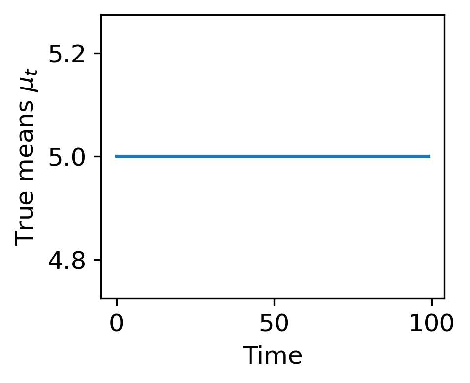
(a) Example 5.1

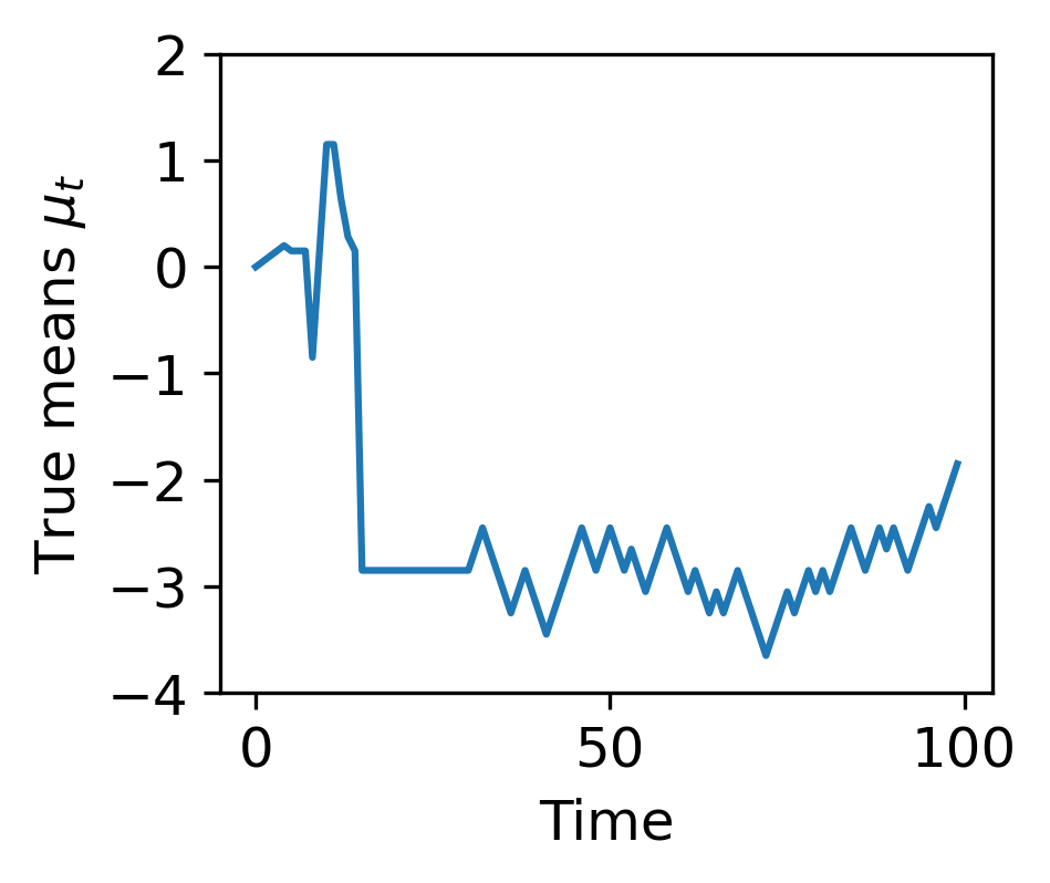
(b) Example 5.2

Figure 1: True means $\{\mu_{t}\}_{t=0}^{100}$ in synthetic data.

Example 5.1.

Figure 1(a) illustrates the stationary case where the true mean stays constant. We explore both low- and high-variance regimes with $\sigma^{2}=1$ and $10$. Table 1 records the average excess risks over 100 periods and 20 independent trials for $\mathcal{V}_{\rm ARW}$ and $\{\mathcal{V}_{k}\}_{k\in I}$. The first and second rows correspond to small and large $\sigma^{2}$. In both regimes, the adaptive $\mathcal{V}_{\rm ARW}$ can leverage the underlying stationarity, yielding excess risks comparable to using the larger $k$’s, whereas the smaller windows perform worse. In Figure 2, we plot the average excess risks over 20 trials at each time $t$ for $\mathcal{V}_{\rm ARW},\mathcal{V}_{1},\mathcal{V}_{256}$ in red, orange and blue.

Table 1: Mean excess risks of selection methods for Example 5.1.

$\mathcal{V}_{\rm ARW}$	$\mathcal{V}_{1}$	$\mathcal{V}_{4}$	$\mathcal{V}_{16}$	$\mathcal{V}_{64}$	$\mathcal{V}_{256}$
0.015	0.043	0.025	0.013	0.010	0.010
1.293	4.117	2.572	1.396	1.015	0.982

Example 5.2.

We carry out the same experiments in a scenario with sufficient non-stationarity. The true means $\{\mu_{t}\}_{t=1}^{100}$ in Figure 1(b) are generated using a randomized mechanism. See Section C.1 for a detailed description. Similar to that of Example 1, Table 2 summarizes the mean excess risks. When $\sigma^{2}=1$, the non-stationary of the underlying means is largely preserved, and $\mathcal{V}_{\rm ARW}$ outperforms all other $\mathcal{V}_{w}$’s, demonstrating its adaptive abilities. When $\sigma^{2}=10$, the large noise makes the non-stationarity less significant, so $\mathcal{V}_{w}$ with a larger $w$ will be more stable. Nevertheless, $\mathcal{V}_{\rm ARW}$ maintains a competitive performance. We also plot the average excess risks over 20 trials at each time $t$ in Figure 3.

Table 2: Mean excess risks of selection methods for Example 5.2.

$\mathcal{V}_{\rm ARW}$	$\mathcal{V}_{1}$	$\mathcal{V}_{4}$	$\mathcal{V}_{16}$	$\mathcal{V}_{64}$	$\mathcal{V}_{256}$
0.139	0.157	0.171	0.539	1.034	1.067
2.052	4.425	2.934	1.920	1.771	1.784

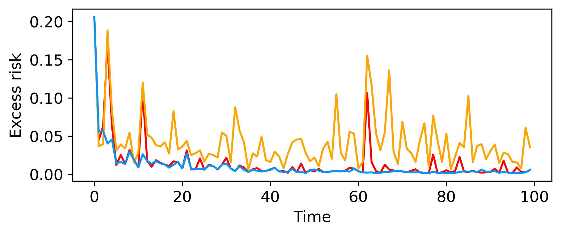
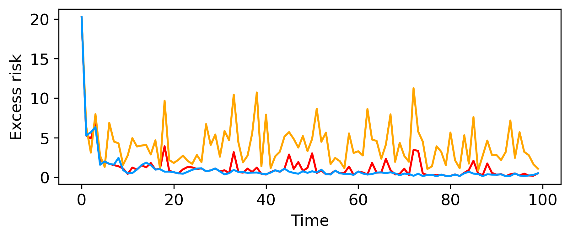
Figure 2: Excess risks in Example 1: $\sigma^{2}=1$ (up) and $\sigma^{2}=10$ (down). Red: $\mathcal{V}_{\rm ARW}$. Orange: $\mathcal{V}_{1}$. Blue: $\mathcal{V}_{256}$.

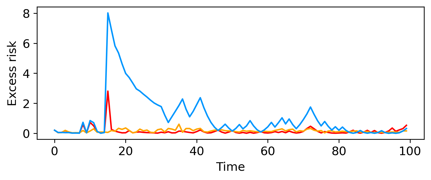
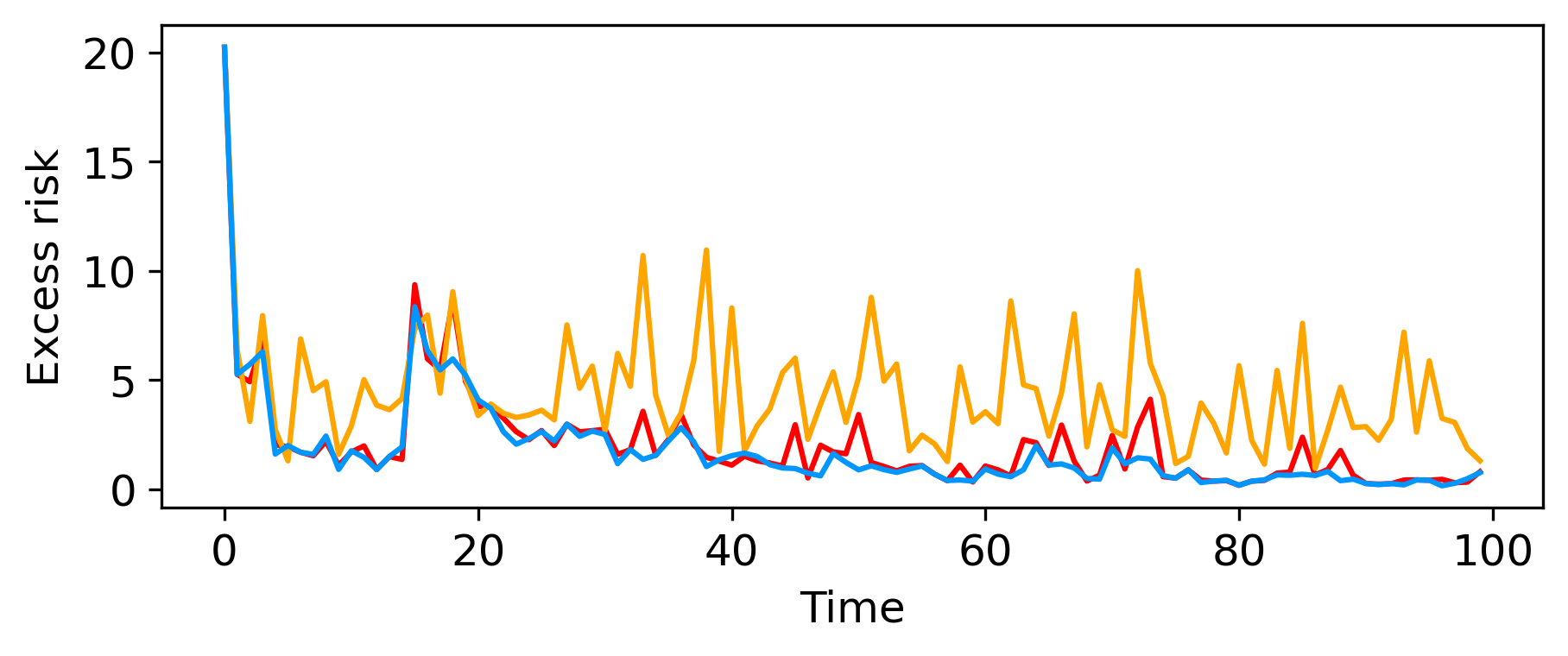
Figure 3: Excess risks in Example 2: $\sigma^{2}=1$ (up) and $\sigma^{2}=10$ (down). Red: $\mathcal{V}_{\rm ARW}$. Orange: $\mathcal{V}_{1}$. Blue: $\mathcal{V}_{256}$.

5.2 Real Data: Topic Frequency Estimation

We now analyze a real-world dataset collected from arXiv.org, which contains basic information of the submitted papers, such as title, abstract and categories. We study the topics of papers in the category cs.LG from March $1$st, $2020$ to December $31$st, $2023$. There are $118,883$ papers in total, and we would like to estimate the proportion of deep learning papers in this category. Each week is a time period, and there are $200$ weeks in total. We regard a paper as a deep learning paper if its abstract contains at least one of the words “deep”, “neural”, “dnn” and “dnns”. The data in each period is randomly split into training, validation and test sets. The training set $\mathcal{B}_{j}^{\rm tr}$ has $15$ samples, the validation set $\mathcal{B}_{j}^{\rm va}$ has $5$ samples and the rest of the samples $\mathcal{B}_{j}^{\rm te}$ are used for testing. Typically $|\mathcal{B}_{j}^{\rm te}|\in[300,1200]$. In Figure 6(a), we plot the frequencies over $200$ weeks estimated from $\{\mathcal{B}_{j}^{\rm te}\}_{j=1}^{200}$, which exhibits a slowly drifting pattern.

In each period $t$, we construct $5$ estimates $\{{\mathcal{T}}(t,w)\}_{w\in I}$, where ${\mathcal{T}}(t,w)$ computes the average frequency from the data $\{\mathcal{B}_{j}^{\rm tr}\}_{j=t-w\wedge t+1}^{t}$. The selection procedure is similar to that in the synthetic data experiment. To measure the quality of the selected model, we compute its excess risk (equivalent to squared estimation error) using $\mathcal{B}_{t}^{\rm te}$. We compare $\mathcal{V}_{\rm ARW}$ with the fixed-window benchmarks $\{\mathcal{V}_{k}\}_{k\in I}$. The average excess risks over 200 weeks and 20 independent runs are listed in Table 3. In Figure 4, we also plot the excess risks in every period. We observe that the performance of $\mathcal{V}_{\rm ARW}$ is comparable to that of the large-window benchmark $\mathcal{V}_{256}$, while the small-window model selection algorithm $\mathcal{V}_{1}$ performs poorly.

Table 3: Overall average excess risks ($\times 10^{-3}$) of selection methods on the arXiv data.

$\mathcal{V}_{\rm ARW}$	$\mathcal{V}_{1}$	$\mathcal{V}_{4}$	$\mathcal{V}_{16}$	$\mathcal{V}_{64}$	$\mathcal{V}_{256}$
2.4	6.7	4.5	2.4	1.7	1.9

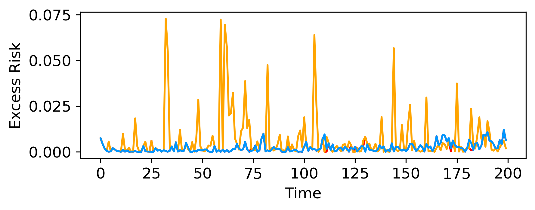
Figure 4: Error curves of different model selection methods on the arXiv data. Red: $\mathcal{V}_{\rm ARW}$. Orange: $\mathcal{V}_{1}$. Blue: $\mathcal{V}_{256}$.

5.3 Real Data: Housing Price Prediction

Finally, we test our method using a real estate dataset maintained by the Dubai Land Department. We study sales of apartments during the past 16 years (from January 1st, 2008 to December 31st, 2023). There are 211,432 samples (sales) in total, and we want to predict the final price given characteristics of an apartment (e.g., number of rooms, size, location). Each month is treated as a time period, and there are 192 of them in total. Our goal is to build a prediction model for each period using historical data. In Figure 6(b), we plot the monthly average prices. Compared with the arXiv data, the distribution shift in this case is more abrupt.

The data in each period is randomly split into training, validation and test sets with proportions 60%, 20% and 20%, respectively. We follow the standard practice to apply a logarithmic transform to the price and target that in our prediction. See Section C.3 for other details of preprocessing.

Table 4: Overall MSE of different methods on the housing data.

$\mathcal{V}_{\rm ARW}$	$\mathcal{V}_{1}$	$\mathcal{V}_{4}$	$\mathcal{V}_{16}$	$\mathcal{V}_{64}$	$\mathcal{V}_{256}$
0.072	0.072	0.071	0.072	0.090	0.095

For the $t$-th period, we use each of the 5 training windows $w\in I$ to perform random forest regression on training data $\{\mathcal{B}_{j}^{\rm tr}\}_{j=t-w\wedge t+1}^{t}$. This results in models $\{{\mathcal{T}}(t,w)\}_{w\in I}$. One of them is selected using validation data and finally evaluated on the test data $\mathcal{B}_{t}^{\rm te}$ by the mean squared error (MSE). For each model selection method, we compute the average MSE over all of the 192 time periods and 20 independent runs. We compare our proposed approach with fixed-window benchmarks $\{\mathcal{V}_{k}\}_{k\in I}$. The mean values are reported in Table 4. In addition, we also plot the test MSEs of our method, $\mathcal{V}_{1}$ and $\mathcal{V}_{256}$ in all individual time periods, see Figure 5. Due to the strong non-stationarity, model selection based on large windows does not work well. Our method still nicely adapts to the changes.

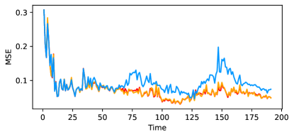
Figure 5: Error curves of different model selection methods on the housing data. Red: $\mathcal{V}_{\rm ARW}$. Orange: $\mathcal{V}_{1}$. Blue: $\mathcal{V}_{256}$.

6 Discussions

We developed adaptive window approaches to model assessment and selection in a changing environment. Theoretical analyses and numerical experiments demonstrate their adaptivity to unknown temporal distribution shift. Several further directions are worth exploring. First, our algorithms and analyses only apply to bounded losses. It is important both theoretically and practically to extend them to unbounded loss functions. Second, our model selection algorithm attains a fast rate in the setting of bounded regression without covariate shift. A natural question is whether a fast rate can still be achieved in other scenarios such as classification. Finally, another interesting direction is to extend our model selection algorithm to infinite model classes.

Appendix A Proofs for Section 3

A.1 Proof of Lemma 3.1

Inequality (2.10) in Boucheron et al. (2013) implies that for any $t\geq 0$,

$$\mathbb{P}\bigg{(}\frac{1}{n}\sum_{i=1}^{n}(x_{i}-\mathbb{E}x_{i})>t\bigg{)}\leq\exp\left(-\frac{nt^{2}/2}{\sigma^{2}+(b-a)t/3}\right).$$

Fix $\delta\in(0,1)$. Then,

$$\quad\exp\left(-\frac{nt^{2}/2}{\sigma^{2}+(b-a)t/3}\right)\leq\delta$$

$$\Leftrightarrow \quad\frac{nt^{2}}{2}\geq\sigma^{2}\log(1/\delta)+\frac{t(b-a)\log(1/\delta)}{3}$$

$$\Leftrightarrow \quad\frac{n}{2}\bigg{(}t-\frac{(b-a)\log(1/\delta)}{3n}\bigg{)}^{2}\geq\sigma^{2}\log(1/\delta)+\frac{n}{2}\bigg{(}\frac{(b-a)\log(1/\delta)}{3n}\bigg{)}^{2}$$

$$\Leftarrow \quad\bigg{(}t-\frac{(b-a)\log(1/\delta)}{3n}\bigg{)}^{2}\geq\bigg{(}\sigma\sqrt{\frac{2\log(1/\delta)}{n}}+\frac{(b-a)\log(1/\delta)}{3n}\bigg{)}^{2}$$

$$\Leftarrow \quad t\geq\sigma\sqrt{\frac{2\log(1/\delta)}{n}}+\frac{2(b-a)\log(1/\delta)}{3n}.$$

Hence,

$$\mathbb{P}\left(\frac{1}{n}\sum_{i=1}^{n}(x_{i}-\mathbb{E}x_{i})>\sigma\sqrt{\frac{2\log(1/\delta)}{n}}+\frac{2(b-a)\log(1/\delta)}{3n}\right)\leq\delta.$$

Replacing each $x_{i}$ by $-x_{i}$ gives bounds on the lower tail and the absolute deviation.

A.2 Proof of Lemma 3.2

The result is trivial when $B_{t,k}=1$ (i.e. $k=B_{t}=1$), as $\widehat{\psi}(t,k,\delta)=\psi(t,k,\delta)$. From now on, we assume that $B_{t,k}\geq 2$. We first present a useful lemma.

Lemma A.1.

Let $\{x_{i}\}_{i=1}^{n}$ be independent, $[0,1]$-valued random variables. Define the sample mean $\widehat{\mu}=\frac{1}{n}\sum_{i=1}^{n}x_{i}$ and the sample variance $\widehat{v}^{2}=\frac{1}{n-1}\sum_{i=1}^{n}(x_{i}-\widehat{\mu})^{2}$. Let $\mu=\frac{1}{n}\sum_{i=1}^{n}\mathbb{E}x_{i}$ and $v^{2}=\mathbb{E}\widehat{v}^{2}$. We have

$$v^{2}=\frac{1}{n-1}\sum_{i=1}^{n}(\mathbb{E}x_{i}-\mu)^{2}+\frac{1}{n}\sum_{i=1}^{n}\operatorname{{\rm var}}(x_{i})$$

and for any $\delta\in(0,1)$,

$$\mathbb{P}\bigg{(}v\leq\widehat{v}+\sqrt{\frac{2\log(1/\delta)}{n-1}}\bigg{)}\geq 1-\delta\qquad\text{and}\qquad\mathbb{P}\bigg{(}v\geq\widehat{v}-\sqrt{\frac{2\log(1/\delta)}{n-1}}\bigg{)}\geq 1-\delta.$$

Proof of Lemma A.1.

Define $\bm{x}=(x_{1},\cdots,x_{n})^{\top}$, $\bm{\mu}=\mathbb{E}\bm{x}$ and $\bm{\Sigma}={\rm diag}(\operatorname{{\rm var}}(x_{1}),\cdots,\operatorname{{\rm var}}(x_{n}))$. Let $\bm{1}_{n}$ be the $n$-dimensional all-one vector. We have $\widehat{\mu}=\bm{1}_{n}^{\top}\bm{x}/n$ and

$$\sum_{i=1}^{n}(x_{i}-\widehat{\mu})^{2}=\|(\bm{I}-\bm{1}_{n}\bm{1}_{n}^{\top}/n)\bm{x}\|_{2}^{2}=\bm{x}^{\top}(\bm{I}-\bm{1}_{n}\bm{1}_{n}^{\top}/n)\bm{x}.$$

Then,

$$(n-1)\mathbb{E}\widehat{v}^{2} =\langle\bm{\mu}\bm{\mu}^{\top}+\bm{\Sigma},\bm{I}-\bm{1}_{n}\bm{1}_{n}^{\top}/n\rangle=\bm{\mu}^{\top}(\bm{I}-\bm{1}_{n}\bm{1}_{n}^{\top}/n)\bm{\mu}+\langle\bm{\Sigma},\bm{I}-\bm{1}_{n}\bm{1}_{n}^{\top}/n\rangle$$

$$=\sum_{i=1}^{n}(\mathbb{E}x_{i}-\mu)^{2}+\bigg{(}1-\frac{1}{n}\bigg{)}\sum_{i=1}^{n}\operatorname{{\rm var}}(x_{i}).$$

This verifies the expression of $v^{2}$. The concentration bounds come from Theorem 10 in Maurer and Pontil (2009). ∎

We now come back to Lemma 3.2. It suffices to consider the special case $b-a=1$. From Lemma A.1 we immediately get $\mathbb{E}\widehat{v}_{t,k}^{2}=v_{t,k}^{2}$, where

$$v_{t,k}^{2}=\sigma^{2}_{t,k}+\frac{1}{B_{t,k}-1}\sum_{j=t-k+1}^{t}B_{j}(\mu_{j}-\mu_{t,k})^{2}.$$ (A.1)

In addition, for any $\delta\in(0,1)$,

$$\mathbb{P}\left(v_{t,k}\leq\widehat{v}_{t,k}+\sqrt{\frac{2\log(1/\delta)}{B_{t,k}-1}}\right)\geq 1-\delta\qquad\text{and}\qquad\mathbb{P}\left(v_{t,k}\geq\widehat{v}_{t,k}-\sqrt{\frac{2\log(1/\delta)}{B_{t,k}-1}}\right)\geq 1-\delta.$$

With probability at least $1-\delta$, we have $\sigma_{t,k}\leq v_{t,k}\leq\widehat{v}_{t,k}+\sqrt{\frac{2\log(1/\delta)}{B_{t,k}-1}}$ and thus

$$\psi(t,k,\delta) \leq\left(\widehat{v}_{t,k}+\sqrt{\frac{2\log(1/\delta)}{B_{t,k}-1}}\right)\sqrt{\frac{2\log(2/\delta)}{B_{t,k}}}+\frac{2\log(2/\delta)}{3(B_{t,k}-1)}$$

$$\leq\widehat{v}_{t,k}\sqrt{\frac{2\log(2/\delta)}{B_{t,k}}}+\frac{8\log(2/\delta)}{3(B_{t,k}-1)}=\widehat{\psi}(t,k,\delta).$$

To prove the second bound, note that

$$v_{t,k} =\bigg{(}\sigma^{2}_{t,k}+\frac{1}{B_{t,k}-1}\sum_{j=t-k+1}^{t}B_{j}(\mu_{j}-\mu_{t,k})^{2}\bigg{)}^{1/2}$$

$$\leq\sigma_{t,k}+\bigg{(}\frac{1}{B_{t,k}-1}\sum_{j=t-k+1}^{t}B_{j}(\mu_{j}-\mu_{t,k})^{2}\bigg{)}^{1/2}$$

$$=\sigma_{t,k}+\sqrt{\frac{B_{t,k}}{B_{t,k}-1}}\cdot\bigg{(}\frac{1}{B_{t,k}}\sum_{j=t-k+1}^{t}B_{j}(\mu_{j}-\mu_{t})^{2}\bigg{)}^{1/2}$$

$$\leq\sigma_{t,k}+\sqrt{\frac{B_{t,k}}{B_{t,k}-1}}\cdot\max_{t-k+1\leq j\leq t}|\mu_{j}-\mu_{t}|.$$

By Lemma A.1, with probability at least $1-\delta$, we have $v_{t,k}\geq\widehat{v}_{t,k}-\sqrt{\frac{2\log(1/\delta)}{B_{t,k}-1}}$ and thus

$$\widehat{v}_{t,k} \leq v_{t,k}+\sqrt{\frac{2\log(1/\delta)}{B_{t,k}-1}}\leq\sigma_{t,k}+\sqrt{\frac{B_{t,k}}{B_{t,k}-1}}\cdot\max_{t-k+1\leq j\leq t}|\mu_{j}-\mu_{t}|+\sqrt{\frac{2\log(1/\delta)}{B_{t,k}-1}}.$$

As a result,

$$\psi(t,k,\delta) \geq\sigma_{t,k}\sqrt{\frac{2\log(2/\delta)}{B_{t,k}}}+\frac{\log(2/\delta)}{3(B_{t,k}-1)}$$

$$\geq\bigg{(}\widehat{v}_{t,k}-\sqrt{\frac{B_{t,k}}{B_{t,k}-1}}\cdot\max_{t-k+1\leq j\leq t}|\mu_{j}-\mu_{t}|-\sqrt{\frac{2\log(1/\delta)}{B_{t,k}-1}}\bigg{)}\sqrt{\frac{2\log(2/\delta)}{B_{t,k}}}+\frac{\log(2/\delta)}{3(B_{t,k}-1)}$$

$$\geq\widehat{v}_{t,k}\sqrt{\frac{2\log(2/\delta)}{B_{t,k}}}-\sqrt{\frac{2\log(2/\delta)}{B_{t,k}-1}}\cdot\max_{t-k+1\leq j\leq t}|\mu_{j}-\mu_{t}|-\frac{5\log(2/\delta)}{3(B_{t,k}-1)}$$

$$=\bigg{(}\widehat{v}_{t,k}\sqrt{\frac{2\log(2/\delta)}{B_{t,k}}}+\frac{8\log(2/\delta)}{3(B_{t,k}-1)}\bigg{)}-\sqrt{\frac{2\log(2/\delta)}{B_{t,k}-1}}\cdot\max_{t-k+1\leq j\leq t}|\mu_{j}-\mu_{t}|-\frac{13\log(2/\delta)}{3(B_{t,k}-1)}$$

$$=\widehat{\psi}(t,k,\delta)-\sqrt{\frac{2\log(2/\delta)}{B_{t,k}-1}}\cdot\max_{t-k+1\leq j\leq t}|\mu_{j}-\mu_{t}|-\frac{13\log(2/\delta)}{3(B_{t,k}-1)}$$

$$\geq\widehat{\psi}(t,k,\delta)-\xi(t,k,\delta).$$

The first and last inequalities follow from the fact that $B_{t,k}\geq 2$.

A.3 Proof of Lemma 3.3

When the event (3.4) happens, for every $i\in[k]$,

$$|\widehat{\mu}_{t,k}-\widehat{\mu}_{t,i}|\leq|\widehat{\mu}_{t,k}-\mu_{t}|+|\widehat{\mu}_{t,i}-\mu_{t}|\leq\left[\phi(t,k)+\widehat{\psi}(t,k,\delta)\right]+\left[\phi(t,i)+\widehat{\psi}(t,i,\delta)\right],$$

so

$$|\widehat{\mu}_{t,k}-\widehat{\mu}_{t,i}|-\left[\widehat{\psi}(t,k,\delta)+\widehat{\psi}(t,i,\delta)\right]\leq\phi(t,k)+\phi(t,i)\leq 2\phi(t,k),$$

where we used $\phi(t,i)\leq\phi(t,k)$. Taking maximum over all $i\in[k]$ gives $\widehat{\phi}(t,k,\delta)\leq 2\phi(t,k)$.

A.4 Proof of Theorem 3.1

We will prove that with probability at least $1-3t\delta$,

$$|\widehat{\mu}_{t,\widehat{k}}-\mu_{t}|\leq 3\min_{k\in[t]}\left\{3\sqrt{\log(2/\delta)}\cdot\max_{t-k+1\leq j\leq t}|\mu_{j}-\mu_{t}|+\sigma_{t,k}\sqrt{\frac{2\log(2/\delta)}{B_{t,k}}}+\frac{10(b-a)\log(2/\delta)}{B_{t,k}}\right\}.$$

By Lemma 3.4,

$$\mathbb{P}\left(|\widehat{\mu}_{t,\widehat{k}}-\mu_{t}|\leq 3\min_{k\in[t]}\left\{\phi(t,k)+\widehat{\psi}(t,k,\delta)\right\}\right)\geq 1-2t\delta.$$ (A.2)

By the second bound in Lemma 3.2,

$$\mathbb{P}\bigg{(}\widehat{\psi}(t,k,\delta)\leq\psi(t,k,\delta^{\prime})+\xi(t,k,\delta),~{}\forall k\in[t]\bigg{)}\geq 1-t\delta.$$ (A.3)

By (A.2), (A.3) and the union bound, we obtain that with probability at least $1-3t\delta$,

$$|\widehat{\mu}_{t,\widehat{k}}-\mu_{t}|\leq 3\min_{k\in[t]}\bigg{\{}\phi(t,k)+\psi(t,k,\delta)+\xi(t,k,\delta)\bigg{\}}.$$

Finally, when $B_{t,k}\geq 2$,

$$\phi(t,k)+\psi(t,k,\delta)+\xi(t,k,\delta)$$

$$\leq\max_{t-k+1\leq j\leq t}|\mu_{j}-\mu_{t}|+\sigma_{t,k}\sqrt{\frac{2\log(2/\delta)}{B_{t,k}}}+\frac{2(b-a)\log(2/\delta)}{3(B_{t,k}-1)}$$

$$\qquad+\sqrt{\frac{4\log(2/\delta)}{B_{t,k}}}\cdot\max_{t-k+1\leq j\leq t}|\mu_{j}-\mu_{t}|+\frac{13(b-a)\log(2/\delta)}{3(B_{t,k}-1)}$$

$$\leq 3\sqrt{\log(2/\delta)}\cdot\max_{t-k+1\leq j\leq t}|\mu_{j}-\mu_{t}|+\sigma_{t,k}\sqrt{\frac{2\log(2/\delta)}{B_{t,k}}}+\frac{5(b-a)\log(2/\delta)}{B_{t,k}-1}$$

$$\leq 3\sqrt{\log(2/\delta)}\cdot\max_{t-k+1\leq j\leq t}|\mu_{j}-\mu_{t}|+\sigma_{t,k}\sqrt{\frac{2\log(2/\delta)}{B_{t,k}}}+\frac{10(b-a)\log(2/\delta)}{B_{t,k}}.$$

When $B_{t,k}=1$, we have $\phi(t,k)+\psi(t,k,\delta)=b-a$, which is dominated by the bound above. This finishes the proof.

Appendix B Proofs for Section 4

B.1 Proof of Lemma 4.1

Fix $k\in[t]$. For every $f\in\{f_{1},f_{2}\}$,

$$L_{t}(f_{\widehat{r}})-L_{t}(f) =\big{[}L_{t}(f_{\widehat{r}_{k}})-\widehat{L}_{t,k}(f_{\widehat{r}_{k}})\big{]}+\big{[}\widehat{L}_{t,k}(f_{\widehat{r}_{k}})-L_{t}(f)\big{]}$$

$$\leq\big{[}L_{t}(f_{\widehat{r}_{k}})-\widehat{L}_{t,k}(f_{\widehat{r}_{k}})\big{]}+\big{[}\widehat{L}_{t,k}(f)-L_{t}(f)\big{]}$$

$$=\big{[}\widehat{L}_{t,k}(f)-\widehat{L}_{t,k}(f_{\widehat{r}_{k}})\big{]}+\big{[}L_{t}(f_{\widehat{r}_{k}})-L_{t}(f)\big{]}$$

$$\leq\bigg{|}\big{[}\widehat{L}_{t,k}(f_{1})-\widehat{L}_{t,k}(f_{2})\big{]}+\big{[}L_{t}(f_{1})-L_{t}(f_{2})\big{]}\bigg{|}.$$

Taking minimum over $f\in\{f_{1},f_{2}\}$ yields

$$L_{t}(f_{\widehat{r}})-\min_{r\in[2]}L_{t}(f_{r})\leq\left|\big{[}\widehat{L}_{t,k}(f_{1})-\widehat{L}_{t,k}(f_{2})\big{]}+\big{[}L_{t}(f_{1})-L_{t}(f_{2})\big{]}\right|.$$

B.2 Proof of Theorem 4.2

We will prove that with probability at least $1-3t\delta$, Algorithm 2 outputs $\widehat{f}$ satisfying

$$\|\widehat{f}-f_{t}^{*}\|_{\mathcal{P}}-\min_{r\in[2]}\|f_{r}-f_{t}^{*}\|_{\mathcal{P}}\leq C^{\prime}\sqrt{\log(2+\delta^{-1})}\min_{k\in[t]}\left\{\max_{t-k+1\leq j\leq t}\|f_{j}^{*}-f_{t}^{*}\|_{\mathcal{P}}+\frac{M}{\sqrt{B_{t,k}}}\right\},$$

where $C^{\prime}>0$ is a universal constant.

Following the notation in Problem 3.1 with $u_{j,i}=\ell(f_{1},z_{j,i})-\ell(f_{2},z_{j,i})$, we define

$$\sigma_{j}^{2}=\operatorname{{\rm var}}(u_{j,1})=\operatorname{{\rm var}}\left(\ell(f_{1},z_{j,1})-\ell(f_{2},z_{j,1})\right)\quad\text{and}\quad\sigma_{t,k}^{2}=\frac{1}{B_{t,k}}\sum_{j=t-k+1}^{t}B_{j}\sigma_{j}^{2}.$$

By Lemma 4.1 and Theorem 3.1, with probability at least $1-3t\delta$,

$$L_{t}(\widehat{f})-\min_{r\in[2]}L_{t}(f_{r})\leq|\widehat{\Delta}_{t,\widehat{k}}-\Delta_{t}|$$

$$\leq 3\min_{k\in[t]}\left\{3\sqrt{\log(2/\delta)}\cdot\max_{t-k+1\leq j\leq t}|\Delta_{j}-\Delta_{t}|+\sigma_{t,k}\sqrt{\frac{2\log(2/\delta)}{B_{t,k}}}+\frac{40M_{0}^{2}\log(2/\delta)}{B_{t,k}}\right\}.$$ (B.1)

From now on suppose that (B.1) happens.

We first derive a bound for $|\Delta_{j}-\Delta_{t}|$. Since

$$\Delta_{j}=\|f_{1}-f_{j}^{*}\|_{\mathcal{P}}^{2}-\|f_{2}-f_{j}^{*}\|_{\mathcal{P}}^{2}=\langle f_{1}-f_{2},f_{1}+f_{2}-2f_{j}^{*}\rangle_{\mathcal{P}},$$

then for every $j\in\mathbb{Z}_{+}$,

$$|\Delta_{j}-\Delta_{t}|=2|\langle f_{1}-f_{2},f_{j}^{*}-f_{t}^{*}\rangle_{\mathcal{P}}|\leq 2\|f_{1}-f_{2}\|_{\mathcal{P}}\|f_{j}^{*}-f_{t}^{*}\|_{\mathcal{P}}.$$

Hence

$$\max_{t-k+1\leq j\leq t}|\Delta_{j}-\Delta_{t}|\leq 2\|f_{1}-f_{2}\|_{\mathcal{P}}\max_{t-k+1\leq j\leq t}\|f_{j}^{*}-f_{t}^{*}\|_{\mathcal{P}}.$$ (B.2)

Next, we bound $\sigma_{t,k}$. We have

$$\sigma_{j}^{2}\leq 2\operatorname{{\rm var}}\left([f_{1}(x_{j,1})-y_{j,1}]^{2}-[f_{j}^{*}(x_{j,1})-y_{j,1}]^{2}\right)+2\operatorname{{\rm var}}\left([f_{2}(x_{j,1})-y_{j,1}]^{2}-[f_{j}^{*}(x_{j,1})-y_{j,1}]^{2}\right).$$

For every $f\in\mathcal{F}$,

$$\operatorname{{\rm var}}\left([f(x_{j,1})-y_{j,1}]^{2}-[f_{j}^{*}(x_{j,1})-y_{j,1}]^{2}\right) \leq\mathbb{E}\left[\left([f(x_{j,1})-y_{j,1}]^{2}-[f_{j}^{*}(x_{j,1})-y_{j,1}]^{2}\right)^{2}\right]$$

$$=\mathbb{E}\left[\left(f(x_{j,1})-f_{j}^{*}(x_{j,1})\right)^{2}\left(f(x_{j,1}+f_{j}^{*}(x_{j,1})-2y_{j,1}\right)^{2}\right]$$

$$\lesssim M_{0}^{2}\|f-f_{j}^{*}\|_{\mathcal{P}}^{2}.$$

Thus,

$$\sigma_{j}\lesssim M_{0}\left(\|f_{1}-f_{j}^{*}\|_{\mathcal{P}}+\|f_{2}-f_{j}^{*}\|_{\mathcal{P}}\right)\lesssim M_{0}\left(\|f_{1}-f_{t}^{*}\|_{\mathcal{P}}+\|f_{2}-f_{t}^{*}\|_{\mathcal{P}}+\|f_{j}^{*}-f_{t}^{*}\|_{\mathcal{P}}\right),$$

which implies

$$\sigma_{t,k}\lesssim M_{0}\left(\|f_{1}-f_{t}^{*}\|_{\mathcal{P}}+\|f_{2}-f_{t}^{*}\|_{\mathcal{P}}+\max_{t-k+1\leq j\leq t}\|f_{j}^{*}-f_{t}^{*}\|_{\mathcal{P}}\right).$$ (B.3)

Substituting (B.2) and (B.3) into (B.1), there exists a universal constant $C>0$ such that for every $k\in[t]$,

$$L_{t}(\widehat{f})-\min_{r\in[2]}L_{t}(f_{r}) \leq C\Bigg{[}\sqrt{\log(2+\delta^{-1})}\left(\|f_{1}-f_{2}\|_{\mathcal{P}}+\frac{M_{0}}{\sqrt{B_{t,k}}}\right)\max_{t-k+1\leq j\leq t}\|f_{j}^{*}-f_{t}^{*}\|_{\mathcal{P}}$$

$$\qquad+M_{0}\sqrt{\frac{\log(2+\delta^{-1})}{B_{t,k}}}\left(\|f_{1}-f_{t}^{*}\|_{\mathcal{P}}+\|f_{2}-f_{t}^{*}\|_{\mathcal{P}}\right)+\frac{M_{0}^{2}\log(2+\delta^{-1})}{B_{t,k}}\Bigg{]}$$

$$=C\bigg{[}2\Phi(t,k)\left(\|f_{1}-f_{t}^{*}\|_{\mathcal{P}}+\|f_{2}-f_{t}^{*}\|_{\mathcal{P}}\right)+\Psi(t,k)\bigg{]},$$ (B.4)

where

$$\Phi(t,k)=\frac{1}{2}\sqrt{\log(2+\delta^{-1})}\left(\max_{t-k+1\leq j\leq t}\|f_{j}^{*}-f_{t}^{*}\|_{\mathcal{P}}+\frac{M_{0}}{\sqrt{B_{t,k}}}\right),$$

$$\Psi(t,k)=M_{0}\sqrt{\frac{\log(2+\delta^{-1})}{B_{t,k}}}\max_{t-k+1\leq j\leq t}\|f_{j}^{*}-f_{t}^{*}\|_{\mathcal{P}}+\frac{M_{0}^{2}\log(2+\delta^{-1})}{B_{t,k}},$$

and we used the triangle inequality $\|f_{1}-f_{2}\|_{\mathcal{P}}\leq\|f_{1}-f_{t}^{*}\|_{\mathcal{P}}+\|f_{2}-f_{t}^{*}\|_{\mathcal{P}}$.

Without loss of generality, assume $L_{t}(f_{1})\geq L_{t}(f_{2})$. When $\widehat{r}_{\widehat{k}}=1$, we have $\widehat{f}=f_{1}$. Then (B.4) yields

$$\|f_{1}-f_{t}^{*}\|_{\mathcal{P}}^{2}-\|f_{2}-f_{t}^{*}\|_{\mathcal{P}}^{2}=L_{t}(\widehat{f})-\min_{r\in[2]}L_{t}(f_{r})\leq C\bigg{[}2\Phi(t,k)\left(\|f_{1}-f_{t}^{*}\|_{\mathcal{P}}+\|f_{2}-f_{t}^{*}\|_{\mathcal{P}}\right)+\Psi(t,k)\bigg{]}.$$

Completing the squares gives

$$\bigg{[}\|f_{1}-f_{t}^{*}\|_{\mathcal{P}}-C\Phi(t,k)\bigg{]}^{2}\leq\bigg{[}\|f_{2}-f_{t}^{*}\|_{\mathcal{P}}+C\Phi(t,k)\bigg{]}^{2}+C\Psi(t,k).$$

Hence

$$\|f_{1}-f_{t}^{*}\|_{\mathcal{P}} \leq\|f_{2}-f_{t}^{*}\|_{\mathcal{P}}+2C\Phi(t,k)+\sqrt{C\Psi(t,k)}$$

$$\leq\|f_{2}-f_{t}^{*}\|_{\mathcal{P}}+C^{\prime}\sqrt{\log(2+\delta^{-1})}\left(\max_{t-k+1\leq j\leq t}\|f_{j}^{*}-f_{t}^{*}\|_{\mathcal{P}}+\frac{M_{0}}{\sqrt{B_{t,k}}}\right)$$

for some universal constant $C^{\prime}>0$. Since this holds for all $k\in[t]$, we get

$$\|\widehat{f}-f_{t}^{*}\|_{\mathcal{P}}-\min_{r\in[2]}\|f_{r}-f_{t}^{*}\|_{\mathcal{P}}$$

$$=\|f_{1}-f_{t}^{*}\|_{\mathcal{P}}-\|f_{2}-f_{t}^{*}\|_{\mathcal{P}}$$

$$\leq C^{\prime}\sqrt{\log(2+\delta^{-1})}\min_{k\in[t]}\left\{\max_{t-k+1\leq j\leq t}\|f_{j}^{*}-f_{t}^{*}\|_{\mathcal{P}}+\frac{M_{0}}{\sqrt{B_{t,k}}}\right\}.$$ (B.5)

We have proved this bound for the case $\widehat{r}_{\widehat{k}}=1$. When $\widehat{r}_{\widehat{k}}=2$, we have $\widehat{f}=f_{2}$ and hence $\|\widehat{f}-f_{t}^{*}\|_{\mathcal{P}}-\min_{r\in[2]}\|f_{r}-f_{t}^{*}\|_{\mathcal{P}}=0$, so the bound (B.5) continues to hold.

B.3 Proof of Theorem 4.3

We will prove that with probability at least $1-3t\delta$, Algorithm 3 outputs $\widehat{f}$ satisfying

$$\|\widehat{f}-f_{t}^{*}\|_{\mathcal{P}}-\min_{r\in[m]}\|f_{r}-f_{t}^{*}\|_{\mathcal{P}}\leq C^{\prime}\sqrt{(\log m)\log(m+\delta^{-1})}\min_{k\in[t]}\left\{\max_{t-k+1\leq j\leq t}\|f_{j}^{*}-f_{t}^{*}\|_{\mathcal{P}}+\frac{M_{0}}{\sqrt{B_{t,k}}}\right\}$$

for some universal constant $C^{\prime}>0$.

Denote Algorithm 2 with data $\{\mathcal{B}_{j}\}_{j=1}^{t}$ by $\mathcal{A}$, which takes as input two models $f^{\prime},f^{\prime\prime}\in\mathcal{F}$ and outputs the selected model $\mathcal{A}(\{f^{\prime},f^{\prime\prime}\})\in\{f^{\prime},f^{\prime\prime}\}$. For notational convenience, we set $\mathcal{A}(\{f\})=f$ for every $f\in\mathcal{F}$. By Theorem 4.2 and the union bound, with probability at least $1-3t\delta$, the following holds for all $f^{\prime},f^{\prime\prime}\in\{f_{r}\}_{r=1}^{m}$:

$$\|\mathcal{A}(\{f^{\prime},f^{\prime\prime}\})-f_{t}^{*}\|_{\mathcal{P}}-\min_{f\in\{f^{\prime},f^{\prime\prime}\}}\|f-f_{t}^{*}\|_{\mathcal{P}}\\ \leq C\sqrt{\log(m+\delta^{-1})}\min_{k\in[t]}\left\{\max_{t-k+1\leq j\leq t}\|f_{j}^{*}-f_{t}^{*}\|_{\mathcal{P}}+\frac{M_{0}}{\sqrt{B_{t,k}}}\right\},$$ (B.6)

where $C>0$ is a universal constant. From now on, suppose that this event happens.

For each $s\in[S+1]$, let

$$g_{s}\in\mathop{\mathrm{argmin}}_{g\in\mathcal{F}_{s}}L_{t}(g)=\mathop{\mathrm{argmin}}_{g\in\mathcal{F}_{s}}\|g-f_{t}^{*}\|_{\mathcal{P}}.$$

Since $\mathcal{F}=\mathcal{F}_{1}\supseteq\cdots\supseteq\mathcal{F}_{S}\supseteq\mathcal{F}_{S+1}=\{\widehat{f}\}$, then

$$\|\widehat{f}-f_{t}^{*}\|_{\mathcal{P}}-\min_{r\in[m]}\|f_{r}-f_{t}^{*}\|_{\mathcal{P}}=\sum_{s=1}^{S}\big{(}\|g_{s+1}-f_{t}^{*}\|_{\mathcal{P}}-\|g_{s}-f_{t}^{*}\|_{\mathcal{P}}\big{)}.$$

For each $s\in[S]$, there exists $i_{s}\in[m_{s}+1]$ such that $g_{s}\in\mathcal{G}_{s,i_{s}}$. Let $\widehat{g}_{s}=\mathcal{A}(\mathcal{G}_{s,i_{s}})$ be the model selected from $\mathcal{G}_{s,i_{s}}$ in Algorithm 3. By (B.6) and the definition of $g_{s}$,

$$\|\widehat{g}_{s}-f_{t}^{*}\|_{\mathcal{P}}-\|g_{s}-f_{t}^{*}\|_{\mathcal{P}}\leq C\sqrt{\log(m+\delta^{-1})}\min_{k\in[t]}\left\{\max_{t-k+1\leq j\leq t}\|f_{j}^{*}-f_{t}^{*}\|_{\mathcal{P}}+\frac{M_{0}}{\sqrt{B_{t,k}}}\right\}.$$

Moreover, since $\widehat{g}_{s}\in\mathcal{F}_{s+1}$, then $\|g_{s+1}-f_{t}^{*}\|_{\mathcal{P}}\leq\|\widehat{g}_{s}-f_{t}^{*}\|_{\mathcal{P}}$. Therefore,

$$\|\widehat{f}-f_{t}^{*}\|_{\mathcal{P}}-\min_{r\in[m]}\|f_{r}-f_{t}^{*}\|_{\mathcal{P}} =\sum_{s=1}^{S}\big{(}\|g_{s+1}-f_{t}^{*}\|_{\mathcal{P}}-\|g_{s}-f_{t}^{*}\|_{\mathcal{P}}\big{)}$$

$$\leq\sum_{s=1}^{S}\big{(}\|\widehat{g}_{s}-f_{t}^{*}\|_{\mathcal{P}}-\|g_{s}-f_{t}^{*}\|_{\mathcal{P}}\big{)}$$

$$\leq\sum_{s=1}^{S}C\sqrt{\log(m+\delta^{-1})}\min_{k\in[t]}\left\{\max_{t-k+1\leq j\leq t}\|f_{j}^{*}-f_{t}^{*}\|_{\mathcal{P}}+\frac{M_{0}}{\sqrt{B_{t,k}}}\right\}$$

$$\leq C^{\prime}\sqrt{(\log m)\log(m+\delta^{-1})}\min_{k\in[t]}\left\{\max_{t-k+1\leq j\leq t}\|f_{j}^{*}-f_{t}^{*}\|_{\mathcal{P}}+\frac{M_{0}}{\sqrt{B_{t,k}}}\right\}$$

for some universal constant $C^{\prime}>0$.

Appendix C Numerical Experiments: Additional Details

C.1 Example 5.2 of the Synthetic Data

We give an outline of how the true mean sequence $\{\mu_{t}\}$ used in Figure 1(b) is generated. The sequence is constructed by combining 4 parts, each representing a distribution shift pattern. In the first part, we create big shifts in the sequence values. Then, we switch to a sinusoidal pattern. Following that, we introduce a horizontal line. Finally, we will take a random step every period, where the step sizes are independently sampled from $\{1,-1\}$ with equal probability and scaled with a constant. The function takes in 3 parameters $(N,n,seed)$ where $N$ is the total number of periods, $n$ is the parameter determining the splitting points of the 4 parts, and $seed$ is the random seed we use for code reproducibility. In our experiment, we used $N=100$, $n=2$, and $seed=2024$. The exact function can be found in our code.

C.2 Non-Stationarity in arXiv and Housing Data

See Figure 6(a) and Figure 6(b).

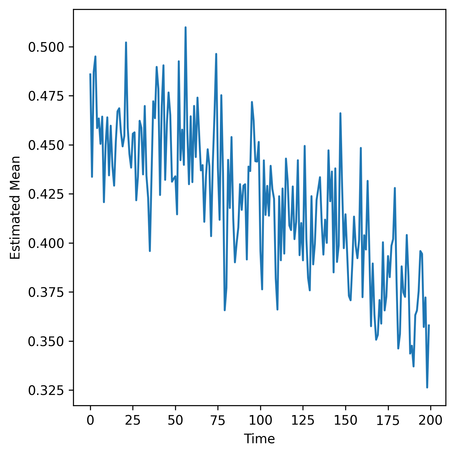
(a) arXiv data

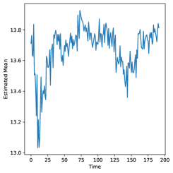
(b) Dubai housing data

Figure 6: Two patterns of temporal distribution shift: slow drift and abrupt changes.

C.3 Experiment on the Housing Data

We focus on transactions of studios and apartments with 1 to 4 bedrooms, between January 1st, 2008 and December 31st, 2023. We import variables instance_date (transaction date), area_name_en (English name of the area where the apartment is located in), rooms_en (number of bedrooms), has_parking (whether or not the apartment has a parking spot), procedure_area (area in the apartment), actual_worth (final price) from the data.

We use instance_date (transaction date) to construct monthly datasets. The target for prediction is the logarithmic of actual_worth. The predictors are area_name_en, rooms_en, has_parking and procedure_area. area_name_en has 58 possible values and encoded as an integer variable.

We remove a sample if its actual_worth or procedure_area is among the largest or smallest 2.5% of the population, whichever is true. After the procedure, $91.6\%$ of the data remain.

We run random forest regression using the function RandomForestRegressor in the Python library scikit-learn. We set random_state = 0 and do not change any other default parameters.

References

- Audibert et al. (2007) Audibert, J.-Y., Munos, R. and Szepesvári, C. (2007). Tuning bandit algorithms in stochastic environments. In Algorithmic Learning Theory (M. Hutter, R. A. Servedio and E. Takimoto, eds.). Springer Berlin Heidelberg, Berlin, Heidelberg.
- Bai et al. (2022) Bai, Y., Zhang, Y.-J., Zhao, P., Sugiyama, M. and Zhou, Z.-H. (2022). Adapting to online label shift with provable guarantees. Advances in Neural Information Processing Systems 35 29960–29974.
-
Besbes et al. (2015)
Besbes, O., Gur, Y. and Zeevi, A. (2015).
Non-stationary stochastic optimization.
Operations Research 63 1227–1244.
URL http://www.jstor.org/stable/24540443 - Bifet and Gavalda (2007) Bifet, A. and Gavalda, R. (2007). Learning from time-changing data with adaptive windowing. In Proceedings of the 2007 SIAM international conference on data mining. SIAM.
-
Boucheron et al. (2013)
Boucheron, S., Lugosi, G. and Massart, P. (2013).
Concentration Inequalities: A Nonasymptotic Theory of
Independence.
Oxford University Press.
URL https://doi.org/10.1093/acprof:oso/9780199535255.001.0001 -
Daniely et al. (2015)
Daniely, A., Gonen, A. and Shalev-Shwartz, S.
(2015).
Strongly adaptive online learning.
In Proceedings of the 32nd International Conference on
Machine Learning (F. Bach and D. Blei, eds.), vol. 37 of Proceedings
of Machine Learning Research. PMLR, Lille, France.
URL https://proceedings.mlr.press/v37/daniely15.html -
Gama et al. (2014)
Gama, J. a., Žliobaitundefined, I., Bifet, A.,
Pechenizkiy, M. and Bouchachia, A. (2014).
A survey on concept drift adaptation.
ACM Comput. Surv. 46.
URL https://doi.org/10.1145/2523813 - Gibbs and Candes (2021) Gibbs, I. and Candes, E. (2021). Adaptive conformal inference under distribution shift. Advances in Neural Information Processing Systems 34 1660–1672.
- Goldenshluger and Lepski (2008) Goldenshluger, A. and Lepski, O. (2008). Universal pointwise selection rule in multivariate function estimation .
- Hanneke et al. (2015) Hanneke, S., Kanade, V. and Yang, L. (2015). Learning with a drifting target concept. In Algorithmic Learning Theory (K. Chaudhuri, C. GENTILE and S. Zilles, eds.). Springer International Publishing, Cham.
- Hastie et al. (2009) Hastie, T., Tibshirani, R., Friedman, J. H. and Friedman, J. H. (2009). The elements of statistical learning: data mining, inference, and prediction, vol. 2. Springer.
- Hazan and Seshadhri (2009) Hazan, E. and Seshadhri, C. (2009). Efficient learning algorithms for changing environments. In Proceedings of the 26th annual international conference on machine learning.
- Huang and Wang (2023) Huang, C. and Wang, K. (2023). A stability principle for learning under non-stationarity. arXiv preprint arXiv:2310.18304 .
-
Jadbabaie et al. (2015)
Jadbabaie, A., Rakhlin, A., Shahrampour, S. and
Sridharan, K. (2015).
Online Optimization : Competing with Dynamic Comparators.
In Proceedings of the Eighteenth International Conference on
Artificial Intelligence and Statistics (G. Lebanon and S. V. N.
Vishwanathan, eds.), vol. 38 of Proceedings of Machine Learning
Research. PMLR, San Diego, California, USA.
URL https://proceedings.mlr.press/v38/jadbabaie15.html - Littlestone and Warmuth (1994) Littlestone, N. and Warmuth, M. K. (1994). The weighted majority algorithm. Information and computation 108 212–261.
- Maurer and Pontil (2009) Maurer, A. and Pontil, M. (2009). Empirical Bernstein bounds and sample variance penalization. In Conference on Learning Theory.
- Mazzetto et al. (2023) Mazzetto, A., Esfandiarpoor, R., Upfal, E. and Bach, S. H. (2023). An adaptive method for weak supervision with drifting data. arXiv preprint arXiv:2306.01658 .
-
Mazzetto and Upfal (2023)
Mazzetto, A. and Upfal, E. (2023).
An adaptive algorithm for learning with unknown distribution drift.
In Thirty-seventh Conference on Neural Information Processing
Systems.
URL https://openreview.net/forum?id=exiXmAfuDK - Mohri and Muñoz Medina (2012) Mohri, M. and Muñoz Medina, A. (2012). New analysis and algorithm for learning with drifting distributions. In Algorithmic Learning Theory: 23rd International Conference, ALT 2012, Lyon, France, October 29-31, 2012. Proceedings 23. Springer.
-
Niu et al. (2016)
Niu, Y. S., Hao, N. and Zhang, H. (2016).
Multiple change-point detection: A selective overview.
Statistical Science 31 611–623.
URL http://www.jstor.org/stable/26408091 - Quinonero-Candela et al. (2022) Quinonero-Candela, J., Sugiyama, M., Schwaighofer, A. and Lawrence, N. D. (2022). Dataset Shift in Machine Learning. MIT Press.
-
Truong et al. (2020)
Truong, C., Oudre, L. and Vayatis, N. (2020).
Selective review of offline change point detection methods.
Signal Processing 167 107299.
URL https://www.sciencedirect.com/science/article/pii/S0165168419303494 -
Wei and Luo (2021)
Wei, C.-Y. and Luo, H. (2021).
Non-stationary reinforcement learning without prior knowledge: an
optimal black-box approach.
In Proceedings of Thirty Fourth Conference on Learning
Theory (M. Belkin and S. Kpotufe, eds.), vol. 134 of Proceedings of
Machine Learning Research. PMLR.
URL https://proceedings.mlr.press/v134/wei21b.html