Are Semi-Dense Detector-Free Methods Good at Matching Local Features?

Abstract

Semi-dense detector-free approaches (SDF), such as LoFTR, are currently among the most popular image matching methods. While SDF methods are trained to establish correspondences between two images, their performances are almost exclusively evaluated using relative pose estimation metrics. Thus, the link between their ability to establish correspondences and the quality of the resulting estimated pose has thus far received little attention. This paper is a first attempt to study this link. We start with proposing a novel structured attention-based image matching architecture (SAM). It allows us to show a counter-intuitive result on two datasets (MegaDepth and HPatches): on the one hand SAM either outperforms or is on par with SDF methods in terms of pose/homography estimation metrics, but on the other hand SDF approaches are significantly better than SAM in terms of matching accuracy. We then propose to limit the computation of the matching accuracy to textured regions, and show that in this case SAM often surpasses SDF methods. Our findings highlight a strong correlation between the ability to establish accurate correspondences in textured regions and the accuracy of the resulting estimated pose/homography. Our code will be made available.

LoFTR+QuadTree            SAM (ours)

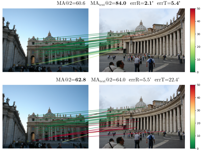
Figure 1: Given query locations within textured regions of the source image (left), we show their predicted correspondents in the target image (right) for: (Top row) SAM (Proposed) - Structured Attention-based image Matching, (Bottom row) LoFTR [Sun et al., 2021]+QuadTree [Tang et al., 2022] - a semi-dense detector-free approach (line colors indicate the distance in pixels with respect to the ground truth correspondent). We report: (MA@2) - the matching accuracy at 2 pixels computed on all the semi-dense locations of the source image with available ground truth correspondent (which includes both textured and uniform regions), (MA${}_{\text{text}}$@2) - the matching accuracy at 2 pixels computed on all the textured semi-dense locations of the source image with available ground truth correspondent (i.e., uniform regions are ignored), (errR and errT) - the relative pose error. SAM has a better pose estimation but a lower matching accuracy (MA@2), which seems counter-intuitive. However, if we consider only textured regions (MA${}_{\text{text}}$@2), then SAM outperforms LoFTR+QuadTree.

1 Introduction

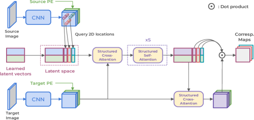
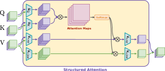
(a) SAM architecture	(b) Structured Attention

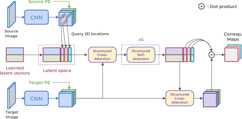
(a) SAM architecture

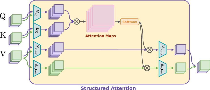
(b) Structured Attention

Figure 2: RG: Overview of the proposed Perceiver-based On-Demand (SAM) method. (Left) The matching architecture is simple and efficient using attention mechanisms, without any dense attention layer (at any resolution), contrary to SDF and FCO methods. (Right) For all attentions layers (self, cross) in our architecture, we use a new formulation of the attention mechanism called Structured attention that constrains the lower half of each output vector to only contain a linear transformation of the positional encodings. See text for details.

Figure 3: Overview of the proposed Structured Attention-based image Matching (SAM) method. (a) The matching architecture first extracts features from both source and target images at resolution 1/4. Then it uses a set of learned latent vectors alongside the descriptors of the query locations, and performs an input structured cross-attention with the dense features of the target. The latent space is then processed through a succession of structured self-attention layers. An output structured cross-attention is applied to update the target features with the information from the latent space. Finally, the correspondence maps are obtained using a dot product. (b) Proposed structured attention layer. See text for details.

Image matching is the task of establishing correspondences between two partially overlapping images. It is considered to be a fundamental problem of 3D computer vision, as establishing correspondences is a precondition for several downstream tasks such as structure from motion [Heinly et al., 2015, Schönberger and Frahm, 2016], visual localisation [Svärm et al., 2017, Sattler et al., 2017, Taira et al., 2018] or simultaneous localization and mapping [Strasdat et al., 2011, Sarlin et al., 2022]. Despite the abundant work dedicated to image matching over the last thirty years, this topic remains an unsolved problem for challenging scenarios, such as when images are captured from strongly differing viewpoints [Arnold et al., 2022] [Jin et al., 2020], present occlusions [Sarlin et al., 2022] or feature day-to-night changes [Zhang et al., 2021].

An inherent part of the problem is the difficulty to evaluate image matching methods. In practice, it is often tackled with a proxy task such as relative or absolute camera pose estimation, or 3D reconstruction.
In this context, image matching performances were recently significantly improved with the advent of attention layers [Vaswani et al., 2017]. Cross-attention layers are mainly responsible for this breakthrough [Sarlin et al., 2020] as they enable the local features of detected keypoints in both images to communicate and adjust with respect to each other. Prior siamese architectures [Yi et al., 2016, Ono et al., 2018, Dusmanu et al., 2019], [Revaud et al., 2019], [Germain et al., 2020, Germain et al., 2021] had so far prevented this type of communication. Shortly after this breakthrough, a second significant milestone was reached [Sun et al., 2021] by combining the usage of attention layers [Sarlin et al., 2020] with the idea of having a detector-free method [Rocco et al., 2018, Rocco et al., 2020a, Rocco et al., 2020b, Li et al., 2020], [Zhou et al., 2021, Truong et al., 2021]. In LoFTR [Sun et al., 2021], low-resolution dense cross-attention layers are employed that allow semi-dense low-resolution features of the two images to communicate and adjust to each other. Such a method is said to be detector-free, as it matches semi-dense local features instead of sparse sets of local features coming from detected keypoint locations [Lowe, 1999].

Semi-dense Detector-Free (SDF) methods [Chen et al., 2022, Giang et al., 2023, Wang et al., 2022, Sun et al., 2021], [Mao et al., 2022, Tang et al., 2022], such as LoFTR, are among the best performing image matching approaches in terms of pose estimation metrics. However, to the best of our knowledge, the link between their ability to establish correspondences and the quality of the resulting estimated pose has thus far received little attention. This paper is a first attempt to study this link.

Contributions - We start with proposing a novel Structured Attention-based image Matching architecture (SAM). We evaluate SAM and 6 SDF methods on 3 datasets (MegaDepth - relative pose estimation and matching, HPatches - homography estimation and matching, ETH3D - matching).

We highlight a counter-intuitive result on two datasets (MegaDepth and HPatches): on the one hand SAM either outperforms or is on par with SDF methods in terms of pose/homography estimation metrics, but on the other hand SDF approaches are significantly better than SAM in terms of Matching Accuracy (MA). Here the MA is computed on all the semi-dense locations (of the source image) with available ground truth correspondent, which includes both textured and uniform regions.

We propose to limit the computation of the matching accuracy to textured regions, and show that in this case SAM often surpasses SDF methods. Our findings highlight a strong correlation between the ability to establish accurate correspondences in textured regions and the accuracy of the resulting estimated pose/homography (see Figure 1).

Organization of the paper - Sec. 2 discusses the related work. The proposed SAM architecture is introduced in Sec. 4 and the experiments in Sec. 5.

2 Related work

Since this paper focuses on the link between the ability of SDF methods to establish correspondences and the quality of the resulting estimated pose, we only present SDF methods in this literature review and refer the reader to [Edstedt et al., 2023, Zhu and Liu, 2023, Ni et al., 2023] for a broader literature review. An extended related work section, including [Zhu and Liu, 2023, Ni et al., 2023, yu2023adaptive, Edstedt et al., 2023, jiang2021cotr, tan2022eco], is provided in the supplementary material.

To the best of our knowledge, LoFTR [Sun et al., 2021] was the first method to perform attention-based detector-free matching. A siamese CNN is first applied on the source/target image pair to extract fine dense features of resolution 1/2 and coarse dense features of resolution 1/8. The source and target coarse features are fed into a dense attention-based module, interleaving self-attention layers with cross-attention layers as proposed in [Sarlin et al., 2020]. To reduce the computational complexity of these dense attention layers, Linear Attention [Katharopoulos et al., 2020] is used instead of vanilla softmax attention [Vaswani et al., 2017]. The resulting features are matched to obtain coarse correspondences. Each coarse correspondence is then refined by cropping $5\!\times\!5$ windows into the fine features and applying another attention-based module. Thus for each location of the semi-dense (factor of 1/8) source grid, a correspondent is predicted. In practice, a Mutual Nearest Neighbor (MNN) step is applied at the end of the coarse matching stage to remove outliers.

In [Tang et al., 2022], a QuadTree attention module is proposed to reduce the computational complexity of vanilla softmax attention from quadratic to linear while keeping its power, as opposed to Linear Attention [Katharopoulos et al., 2020] which was shown to underperform on local feature matching [Germain et al., 2022]. The QuadTree attention module is used as a replacement for Linear Attention module in LoFTR. An architecture called ASpanFormer is introduced in [Chen et al., 2022] that employs the same refinement stage as LoFTR but a different coarse stage architecture. Instead of classical cross-attention layers, the coarse stage uses global-local cross-attention layers that have the ability to focus on regions around current potential correspondences. MatchFormer [Wang et al., 2022] proposes an attention-based backbone, interleaving self and cross-attention layers, to progressively transform a tensor of size $2\!\times\!H\!\times\!W\!\times\!3$ into a tensor of size $2\!\times\!\frac{H}{16}\!\times\!\frac{W}{16}\!\times\!C$. Efficient attention layers such as Spatial Efficient Attention [Wang et al., 2021, Xie et al., 2021] and Linear Attention [Katharopoulos et al., 2020] are employed. A feature pyramid network-like decoder [Lin et al., 2017] is used to output a fine tensor of size $2\!\times\!\frac{H}{2}\!\times\!\frac{W}{2}\!\times\!C_{f}$ and a coarse tensor of size $2\!\times\!\frac{H}{8}\!\times\!\frac{W}{8}\!\times\!C_{c}$, and the matching is performed as in LoFTR. TopicFM [Giang et al., 2023] follows the same global architecture as LoFTR with a different coarse stage. Here, topic distributions (latent semantic instances) are inferred from coarse CNN features using cross-attention layers with topic embeddings. These topic distributions are used to augment the coarse CNN features with self and cross-attention layers. In [Mao et al., 2022], a method called 3DG-STFM proposes to train the LoFTR architecture with a student-teacher method. The teacher is first trained on RGB-D image pairs. The teacher model then guides the student model to learn RGB-induced depth information.

3 On-demand matching paradigm

The ability of SDF methods to match local features is thoroughly evaluated against FCO methods, in Sec. 5, and shows that SDF architectures are generally outperformed (see Tab. 6). However, the results also indicate that the FCO approaches, especially COTR, have an unreasonable computational time. This observation raises the following question: Is it possible to design an architecture that reaches similar performances, with a reasonable run time? To address this question, we first need to formalize the ODM paradigm.

MV:

• The question raised is not related to this section. It may make you think that we design this paradigm because it works better for our architecture.

• Reformulate to make it clear that this paradigm it a good evaluation of the feature matching performances of any architecture.

3.1 Definition

Given a set of MV: L 2D query locations $\left\{\mathbf{p}_{\text{s},i}\right\}_{i=1...L}$ in a source image $\mathtt{I}_{\text{s}}$, ODM consists in finding their MV: L 2D correspondent locations $\left\{\hat{\mathbf{p}}_{\text{t},i}\right\}_{i=1...L}$ in a target image $\mathtt{I}_{\text{t}}$. Thus a method $\mathcal{M}$ that implements ODM can be written as follows:

$$\left\{\hat{\mathbf{p}}_{\text{t},i}\right\}_{i=1...L}=\mathcal{M}\left(\mathtt{I}_{\text{s}},\mathtt{I}_{\text{t}},\left\{\mathbf{p}_{\text{s},i}\right\}_{i=1...L}\right).$$ (1)

Let us highlight that SDF and FCO approaches can be viewed as two extreme implementations of ODM. A FCO method implements ODM by predicting the $L$ correspondents $\left\{\hat{\mathbf{p}}_{\text{t},i}\right\}_{i=1...L}$ of $\left\{\mathbf{p}_{\text{s},i}\right\}_{i=1...L}$ independently. This is an extreme implementation as, on the one hand, it makes the approach elegant, but on the other hand, it makes the computational time unreasonable. An SDF approach can be used to implement ODM since its coarse attention-based matching stage produces dense features for the source and target images. Let us recall that at training time, these features are used to compute a coarse 4D correlation volume using a simple dot product between the source and target features to produce coarse dense correspondences. Thus, in the ODM context, for each query $\mathbf{p}_{\text{s},i}$, a feature vector can be interpolated at location $\mathbf{p}_{\text{s},i}$ in the source features, and a simple dot product between this feature vector and the target features allows one to find a coarse correspondent $\hat{\mathbf{p}}_{\text{t},i}$. This correspondence can then be refined by the fine matching stage. This implementation of ODM seems also extreme as it consists in solving the problem for every source image pixels (at a coarse resolution), and then just querying the results for the $L$ query locations using a simple dot product. This analysis will help us to consider a network architecture significantly different from both SDF and FCO architectures. MV: May suggest POD $\implies$ ODM. Reformulate more ODM centered.

3.2 Test set

In order to evaluate the performance of a given method that implements ODM, pairs of source/target images $\left\{\mathtt{I}_{\text{s}_{k}},\mathtt{I}_{\text{t}_{k}}\right\}_{k=1...K}$ with sets of ground truth correspondences $\left\{\mathbf{p}_{\text{s}_{k},i},\mathbf{p}_{\text{t}_{k},i}\right\}_{i=1...L_{k}}$ are needed. However, some MV: special care must be taken with the sets of ground truth correspondences. For a given query location $\mathbf{p}_{\text{s}_{k},i}$, its correspondent $\mathbf{p}_{\text{t}_{k},i}$ might be 1) outside the target image, 2) occluded or 3) covisible. On the one hand, we are mainly interested in evaluating the ability of a given method to find the correspondent $\mathbf{p}_{\text{t}_{k},i}$ of $\mathbf{p}_{\text{s}_{k},i}$, when $\mathbf{p}_{\text{t}_{k},i}$ is covisible. This would speak in favor of building a test set where each $\mathbf{p}_{\text{t}_{k},i}$ is covisible in the target image. On the other hand, building a test set where each $\mathbf{p}_{\text{t}_{k},i}$ is covisible in the target image implies that each $\mathbf{p}_{\text{s}_{k},i}$ conveys a covisibility information (see eq. 3) as input to the method, it indicates the region of the source image that overlaps with the target image. Thus, an architecture that is tailored for ODM (as the architecture we propose in Sec. 4) could leverage that additional information, while SDF and FCO architectures can not. This would lead to unfair comparisons. MV: Reformulate : To avoid this bias and for fair comparaison … To prevent the query locations $\left\{\mathbf{p}_{\text{s},i}\right\}_{i=1...L}$ to convey this information, we opt for a test set where each $\mathbf{p}_{\text{t}_{k},i}$ may or may not be covisible, and add a binary covisibility variable $v_{\text{t}_{k},i}$, where $\left[v_{\text{t}_{k},i}=1\right]$ indicates that $\mathbf{p}_{\text{t}_{k},i}$ is covisible in the target image ($\left[\cdot\right]$ is the Iverson bracket). More precisely, in practice, for each image pair of each test set, we set $L_{k}$ to 64 and randomly sample (uniformly) the number of covisible correspondences between 1 and 32. Consequently, a test set can be defined as follows:

$$\mathcal{D_{\text{test}}}=\left\{\mathtt{I}_{\text{s}_{k}},\mathtt{I}_{\text{t}_{k}},\left\{\mathbf{p}_{\text{s}_{k},i},\mathbf{p}_{\text{t}_{k},i},v_{\text{t}_{k},i}\right\}_{i=1...L_{k}}\right\}_{k=1...K}.$$ (2)

Source Image

Target Image

Average query map

Average latent map

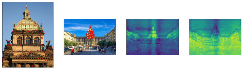
Figure 4: Visualization of the learned latent vectors of SAM. The average query map is obtained by averaging 64 correspondence maps of 64 query locations (Red crosses) while the average latent map is obtained by averaging the 128 correspondence maps of the 128 learned latent vectors. We observe that the average query map is mainly activated around the correspondents, whereas these regions are less activated in the average latent map.

4 Structured attention-based image matching architecture

In the following section, we present our novel Structured Attention-based image Matching architecture (SAM), whose architecture is illustrated in Figure 3.

4.1 Background and notations

Image matching - Given a set of 2D query locations $\left\{\mathbf{p}_{\text{s},i}\right\}_{i=1...L}$ in a source image $\mathtt{I}_{\text{s}}$, we seek to find their 2D correspondent locations $\left\{\hat{\mathbf{p}}_{\text{t},i}\right\}_{i=1...L}$ in a target image $\mathtt{I}_{\text{t}}$:

$$\left\{\hat{\mathbf{p}}_{\text{t},i}\right\}_{i=1...L}=\mathcal{M}\left(\mathtt{I}_{\text{s}},\mathtt{I}_{\text{t}},\left\{\mathbf{p}_{\text{s},i}\right\}_{i=1...L}\right).$$ (3)

Here $\mathcal{M}$ is the image matching method. In the case of semi-dense detector-free methods, the query locations $\left\{\mathbf{p}_{\text{s},i}\right\}_{i=1...L}$ are defined as the source grid locations using a stride of 8. As we will see, SAM is more flexible and can process any set of query locations. However, for a fair comparison, in the experiments all the methods (including SAM) will use source grid locations using a stride of 8 as query locations.

Vanilla softmax attention - A cross-attention operation, with $H$ heads, between a $D$-dimensional query vector $\mathbf{x}$ and a set of $D$-dimensional vectors $\left\{\mathbf{y}_{n}\right\}_{n=1...N}$ can be written as follows:

$$\sum_{h=1}^{H}\sum_{n=1}^{N}{\color[rgb]{0.5,0.5,0.5}\overbrace{{\color[rgb]{0.0,0.0,0}s_{h,n}}}^{1{\times}1}}{\color[rgb]{0.5,0.5,0.5}\overbrace{{\color[rgb]{0.0,0.0,0}\mathtt{W}_{\text{o},h}}}^{D\times D_{H}}}{\color[rgb]{0.5,0.5,0.5}\overbrace{{\color[rgb]{0.0,0.0,0}\mathtt{W}_{\text{v},h}}}^{D_{H}{\times}D}}{\color[rgb]{0.5,0.5,0.5}\overbrace{{\color[rgb]{0.0,0.0,0}\mathbf{y}_{n}}}^{D\times 1}},$$ (4)

where $$\quad s_{h,n}=\frac{\exp({\color[rgb]{0.5,0.5,0.5}\overbrace{{\color[rgb]{0.0,0.0,0}\mathbf{x}^{\top}}}^{1\times D}}{\color[rgb]{0.5,0.5,0.5}\overbrace{{\color[rgb]{0.0,0.0,0}\mathtt{W}_{\text{q},h}^{\top}}}^{D\times D_{H}}}{\color[rgb]{0.5,0.5,0.5}\overbrace{{\color[rgb]{0.0,0.0,0}\mathtt{W}_{\text{k},h}^{\phantom{\top}}}}^{D_{H}\times D}}{\color[rgb]{0.5,0.5,0.5}\overbrace{{\color[rgb]{0.0,0.0,0}\mathbf{y}_{n}^{\top}}}^{D\times 1}})}{\sum_{m=1}^{N}\exp(\mathbf{x}^{\top}\mathtt{W}_{\text{q},h}^{\top}\mathtt{W}_{\text{k},h}\mathbf{y}_{m})}.$$ (5)

In practice, all the matrices $\mathtt{W}_{\cdot,\cdot}$ are learned. Usually $D_{H}=\frac{D}{H}$. The output is a linear combination (with coefficients $s_{h,n}$) of the linearly transformed set of vectors $\left\{\mathbf{y}_{n}\right\}_{n=1...N}$. This operation allows to extract the relevant information in $\left\{\mathbf{y}_{n}\right\}_{n=1...N}$ from the point of view of the query $\mathbf{x}$. The query $\mathbf{x}$ is not an element of that linear combination. As a consequence, a residual connection is often added, usually followed by a layer normalization and a 2-layer MLP (with residual connection) [Vaswani et al., 2017].

In practice, a cross-attention layer between a set of query vectors $\left\{\mathbf{x}_{n}\right\}_{n=1...Q}$ and $\left\{\mathbf{y}_{n}\right\}_{n=1...N}$ is performed in parallel, which is often computationally demanding since, for each head, the coefficients are stored in a $Q\!\times\!N$ matrix. A self-attention layer is a cross-attention layer where $\left\{\mathbf{y}_{n}\right\}_{n=1...N}=\left\{\mathbf{x}_{n}\right\}_{n=1...Q}$.

4.2 Feature extraction stage

Our method takes as input a source image $\mathtt{I}_{\text{s}}$ ($H_{\text{s}}\!\times\!W_{\text{s}}\!\times 3$), a target image $\mathtt{I}_{\text{t}}$ ($H_{\text{t}}\!\times\!W_{\text{t}}\!\times 3$) and a set of 2D query locations ${\left\{\mathbf{p}_{\text{s},i}\right\}_{i=1...L}}$. The first stage of SAM is a classical feature extraction stage. From the source image $\mathtt{I}_{\text{s}}$ ($H_{\text{s}}\!\times\!W_{\text{s}}\!\times 3$) and the target image $\mathtt{I}_{\text{t}}$ ($H_{\text{t}}\!\times\!W_{\text{t}}\!\times 3$), dense visual source features $\mathtt{F}_{\text{s}}$ ($\frac{H_{\text{s}}}{4}\!\times\!\frac{W_{\text{s}}}{4}\!\times 128$) and target features $\mathtt{F}_{\text{t}}$ ($\frac{H_{\text{t}}}{4}\!\times\!\frac{W_{\text{t}}}{4}\!\times 128$) are extracted using a siamese CNN backbone. The Positional Encodings (PE) of the source and target are computed, using an MLP [Sarlin et al., 2020], and concatenated with the visual features of the source and target to obtain two tensors $\mathtt{H}_{\text{s}}$ ($\frac{H_{\text{s}}}{4}\!\times\!\frac{W_{\text{s}}}{4}\!\times 256$) and $\mathtt{H}_{\text{t}}$ ($\frac{H_{\text{t}}}{4}\!\times\!\frac{W_{\text{t}}}{4}\!\times 256$). For each 2D query point $\mathbf{p}_{\text{s},i}$, a descriptor $\mathbf{h}_{\text{s},i}$ of size 256 is extracted from $\mathtt{H}_{\text{s}}$. In practice, we use integer query locations thus there is no need for interpolation here. Technical details concerning this stage are provided in the appendix.

4.3 Latent space attention-based stage

In order to allow for the descriptors ${\left\{\mathbf{h}_{\text{s},i}\right\}_{i=1...L}}$ (at training-time we use $L=1024$) to communicate and adjust with respect to $\mathtt{H}_{\text{t}}$, we draw inspiration from Perceiver [Jaegle et al., 2021, Jaegle et al., 2022], and consider a set of $N\!=\!M\!+\!L$ latent vectors, composed of $M$ learned latent vectors $\left\{\mathbf{m}_{i}\right\}_{i=1...M}$ and the $L$ descriptors $\left\{\mathbf{h}_{\text{s},i}\right\}_{i=1...L}$. These latent vectors $\left\{\left\{\mathbf{m}_{i}\right\}_{i=1...M},\left\{\mathbf{h}_{\text{s},i}\right\}_{i=1...L}\right\}$ are used as queries in an input cross-attention layer to extract the relevant information from $\mathtt{H}_{\text{t}}$, and finally obtain an updated set of latent vectors $\left\{\left\{\mathbf{m}^{(0)}_{i}\right\}_{i=1...M},\left\{\mathbf{h}^{(0)}_{\text{s},i}\right\}_{i=1...L}\right\}$. On the one hand, the outputs $\left\{\mathbf{h}^{(0)}_{\text{s},i}\right\}_{i=1...L}$ contain the information relevant to find their respective correspondents within $\mathtt{H}_{\text{t}}$. On the other hand, the outputs $\left\{\mathbf{m}^{(0)}_{i}\right\}_{i=1...M}$ extracted a general representation of $\mathtt{H}_{\text{t}}$ since they are not aware of the query 2D locations. In practice, we set $M$ to 128. Afterward, a series of $S$ self-attention layers are applied to the latent vectors to get $\left\{\left\{\mathbf{m}^{(S)}_{i}\right\}_{i=1...M},\left\{\mathbf{h}^{(S)}_{\text{s},i}\right\}_{i=1...L}\right\}$. In these layers, all latent vectors can communicate and adjust with respect to each other. For instance, the set $\left\{\mathbf{m}^{(s)}_{i}\right\}_{i=1...M}$ can be used to disambiguate certain correspondences. Then, $\mathtt{H}_{\text{t}}$ is used as a query in an output cross-attention layer to extract the relevant information from the latent vectors. The resulting tensor is written $\mathtt{H}^{\text{out}}_{\text{t}}$. For each updated descriptor $\mathbf{h}^{(S)}_{\text{s},i}$, a correspondence map $\mathtt{C}_{\text{t},i}$ (of size $\frac{H_{\text{t}}}{4}\!\times\!\frac{W_{\text{t}}}{4}$) is obtained by computing the dot product between $\mathbf{h}^{(S)}_{\text{s},i}$ and $\mathtt{H}^{\text{out}}_{\text{t}}$. Finally, for each 2D query location $\mathbf{p}_{\text{s},i}$, the predicted 2D correspondent location $\hat{\mathbf{p}}_{\text{t},i}$ is defined as the argmax of $\mathtt{C}_{\text{t},i}$.

In Figure 4, we propose a visualization of the learned latent vectors of SAM. For visualization purposes, we used $L=64$. Thus the average query map is obtained by averaging the 64 correspondence maps of the 64 query locations, while the average latent map is obtained by averaging the 128 correspondence maps of the 128 learned latent vectors. We observe that the average query map is mainly activated around the correspondents, whereas these regions are less activated in the average latent map.

Source Image                   Target Image               Visio-positional map               Positional map

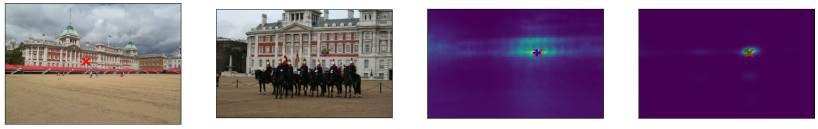
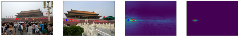
Figure 5: Visualization - Structured attention. The visio-positional and positional maps are computed before the output cross-attention. Red crosses represent the ground-truth correspondences. Blue and Green crosses are the maxima of the visio-positional and positional maps, respectively. One can see that the visio-positional maps are highly multimodal (i.e., sensitive to repetitive structures) while the positional maps are almost unimodal.

4.4 Structured attention

At the end of the feature extraction stage, the upper half of each vector is visual features, while the lower half is positional encodings. In each attention layer (input cross-attention, self-attention and output cross-attention), we found it important to structure the linear transformation matrices $\mathtt{W}_{\text{o},h}$ and $\mathtt{W}_{\text{v},h}$ to constrain the lower half of each output vector to only contain a linear transformation of the positional encodings:

$${\color[rgb]{0.5,0.5,0.5}\overbrace{{\color[rgb]{0.0,0.0,0}\mathtt{W}_{\text{o},h}}}^{D\times D_{H}}}=\bigg{[}{\begin{array}[]{ccc}\lx@intercol\hfil{\color[rgb]{0.5,0.5,0.5}\overbrace{{\color[rgb]{0.0,0.0,0}\mathtt{W}_{\text{o},h,\text{up}}}}^{\frac{D}{2}\times D_{H}}}\hfil\lx@intercol\\ \hline\cr{\color[rgb]{0.5,0.5,0.5}\underbrace{{\color[rgb]{0.0,0.0,0}\mathtt{0}}}_{\ \frac{D}{2}\times\frac{D_{H}}{2}}}&\!|\!&{\color[rgb]{0.5,0.5,0.5}\underbrace{{\color[rgb]{0.0,0.0,0}\mathtt{W}_{\text{o},h,\text{low}}}}_{\frac{D}{2}\times\frac{D_{H}}{2}}}\end{array}}\bigg{]}.$$ (8)

The matrices $\mathtt{W}_{\text{v},h}$ and the fully connected layers within the MLP (at the end of each attention module) are structured the exact same way. Consequently, throughout the network, the lower half of each latent vector only contains transformations of positional encodings, but no visual feature.

In Figure 5 we propose a visualization of two different correspondence maps before the output cross-attention.

The first map is produced using the first 128 dimensions of the feature representation and contains high-level visio-positional features. The second map is produced using the 128 last dimensions of the feature representation and contains only positional encodings. By building these distinct correspondence maps we can observe that while the visio-positional representation is sensitive to repetitive structures, the purely positional representation tends to be only activated in the areas neighbouring the match.

4.5 Loss

At training time, we use a cross-entropy (CE) loss function [Germain et al., 2020] on each correspondence map $\mathtt{C}_{\text{t},i}$ in order to maximise its score at the ground truth location $\mathbf{p}_{\text{t},i}$:

$$\text{CE}\left(\mathtt{C}_{\text{t},i},\mathbf{p}_{\text{t},i}\right)=-\ln\left(\frac{\exp\,\mathtt{C}_{\text{t},i}\left(\mathbf{p}_{\text{t},i}\right)}{\sum_{\mathbf{q}}\exp\,\mathtt{C}_{\text{t},i}\left(\mathbf{q}\right)}\right).$$ (9)

4.6 Refinement

The previously described architecture produces coarse correspondence maps of resolution 1/4. Thus the predicted correspondents ${\left\{\hat{}\mathbf{p}_{\text{t},i}\right\}_{i=1...L}}$ need to be refined. To do so, we simply use a second siamese CNN that outputs dense source and target features at full resolution. For each 2D query location $\mathbf{p}_{\text{s},i}$, a correspondence map is computed on a window of size 11 centered around the coarse prediction. The predicted 2D correspondent location $\hat{\mathbf{p}}_{\text{t},i}$ is defined as the argmax of this correspondence map. This refinement network is trained separately using the same cross-entropy loss eq. 9. Technical details are provided in the appendix.

Table 1: Evaluation on MegaDepth1500 [Sarlin et al., 2020]. We report Matching Accuracy (11) for several thresholds $\eta$, computed on the set of all the semi-dense query locations (source grid with stride 8) with available ground truth correspondents (MA), and on a subset containing only query locations that are within a textured region of the source image (MA${}_{\text{text}}$). Concerning the pose estimation metrics, we report the classical AUC at 5, 10 and 20 degrees. The proposed SAM method outperforms SDF methods in terms of pose estimation, while SDF methods are significantly better in terms of MA. However, when uniform regions are ignored (MA${}_{\text{text}}$), SAM often surpasses SDF methods. These results highlight a strong correlation between the ability to establish precise correspondences in textured regions and the accuracy of the resulting estimated pose.

Method	Matching Accuracy (MA) (11) $\uparrow$							Matching Accuracy							Pose estimation on
								on textured regions (MA${}_{\text{text}}$) (11) $\uparrow$							1/8 grid (AUC) $\uparrow$
	$\eta$=$1$	$\eta$=$2$	$\eta$=$3$	$\eta$=$5$	$\eta$=$10$	$\eta$=$20$		$\eta$=$1$	$\eta$=$2$	$\eta$=$3$	$\eta$=$5$	$\eta$=$10$	$\eta$=$20$		$@5^{\text{o}}$	$@10^{\text{o}}$	$@20^{\text{o}}$
LoFTR [Sun et al., 2021]	49.7	73.2	81.6	87.4	90.5	91.8		55.3	75.2	81.6	86.9	89.9	91.9		52.8	69.2	82.0
MatchFormer [Wang et al., 2022]	51.1	73.4	81.0	86.9	89.5	90.9		56.5	75.6	81.8	87.1	89.6	90.9		52.9	69.7	82.0
TopicFM [Giang et al., 2023]	51.4	75.4	83.7	89.9	92.9	93.5		59.8	77.6	84.8	90.4	92.9	93.7		54.1	70.1	81.6
3DG-STFM[Mao et al., 2022]	51.6	73.7	80.7	86.4	89.0	90.7		57.0	75.8	81.8	86.8	88.8	90.5		52.6	68.5	80.0
ASpanFormer [Chen et al., 2022]	52.0	76.2	84.5	90.7	93.7	94.8		62.2	80.3	85.9	91.0	93.7	94.7		55.3	71.5	83.1
LoFTR+QuadTree [Tang et al., 2022]	51.6	75.9	84.1	90.2	93.1	94.0		61.7	79.9	85.5	90.5	93.3	94.1		54.6	70.5	82.2
SAM (ours)	48.5	70.4	78.0	83.0	85.4	86.4		67.9	83.8	87.3	90.6	93.6	95.2		55.8	72.8	84.2

Table 2: Evaluation on HPatches [Balntas et al., 2017]. We report Matching Accuracy (11) for several thresholds $\eta$, computed on the set of all the semi-dense query locations (source grid with stride 8) with available ground truth correspondents (MA), and on a subset containing only query locations that are within a textured region of the source image (MA${}_{\text{text}}$). Concerning the homography estimation metrics, we report the classical AUC at 3, 5 and 10 pixels. The proposed SAM method is on par with SDF methods in terms of homography estimation, while SDF methods are significantly better in terms of MA. However, when uniform regions are ignored (MA${}_{\text{text}}$), SAM matches SDF performances. These results highlight a strong correlation between the ability to establish precise correspondences in textured regions and the accuracy of the resulting estimated homography.

Method	Matching Accuracy				Matching Accuracy on				Homography estimation
	(MA) (11) $\uparrow$				textured regions (MA${}_{\text{text}}$) (11) $\uparrow$				(AUC) $\uparrow$
	$\eta$=$3$	$\eta$=$5$	$\eta$=$10$		$\eta$=$3$	$\eta$=$5$	$\eta$=$10$		$@3\text{px}$	$@5\text{px}$	$@10\text{px}$
LoFTR [Sun et al., 2021]	66.8	74.3	77.3		67.6	75.3	78.4		65.9	75.6	84.6
MatchFormer [Wang et al., 2022]	66.2	74.9	78.2		67.7	75.8	79.1		65.0	73.1	81.2
TopicFM [Giang et al., 2023]	72.7	85.0	87.5		74.0	86.0	88.5		67.3	77.0	85.7
3DG-STFM[Mao et al., 2022]	64.9	75.1	78.2		66.2	74.3	77.6		64.7	73.1	81.0
ASpanFormer [Chen et al., 2022]	76.2	86.2	88.7		73.9	85.8	88.4		67.4	76.9	85.6
LoFTR+QuadTree [Tang et al., 2022]	70.2	83.1	85.9		73.5	84.3	86.9		67.1	76.1	85.3
SAM (ours)	62.4	70.9	74.2		73.4	86.6	89.3		67.1	76.9	85.9

Table 3: Evaluation on ETH3D [Schöps et al., 2019] for different frame interval sampling rates $r$. We report Matching Accuracy (11) for several thresholds $\eta$, computed on the set of all the semi-dense query locations (source grid with stride 8) with available ground truth correspondents (MA). For ETH3D, ground truth correspondents are based on structure from motion tracks. Consequently, the MA already ignores untextured regions of the source images which explains why SAM is able to outperform SDF methods.

Method	Matching Accuracy (MA) (11) $\uparrow$
	$r=3$						$r=7$						$r=15$
	$\eta$=$1$	$\eta$=$2$	$\eta$=$3$	$\eta$=$5$	$\eta$=$10$		$\eta$=$1$	$\eta$=$2$	$\eta$=$3$	$\eta$=$5$	$\eta$=$10$		$\eta$=$1$	$\eta$=$2$	$\eta$=$3$	$\eta$=$5$	$\eta$=$10$
LoFTR [Sun et al., 2021]	44.8	76.5	88.4	97.0	99.4		39.7	73.1	87.6	95.9	98.5		33.3	66.2	84.8	92.5	96.3
MatchFormer [Wang et al., 2022]	45.5	77.1	89.2	97.2	99.7		40.4	73.8	87.8	96.6	99.0		34.2	66.7	84.9	93.5	97.0
TopicFM [Giang et al., 2023]	45.1	76.9	89.0	97.2	99.6		39.9	73.5	87.9	96.4	99.0		33.8	66.4	85.0	92.8	96.5
3DG-STFM[Mao et al., 2022]	43.9	76.3	88.0	96.9	99.3		39.3	72.7	87.4	95.5	98.3		32.4	65.7	84.7	92.0	96.0
ASpanFormer [Chen et al., 2022]	45.8	77.6	89.6	97.8	99.8		40.6	73.8	88.1	96.8	99.0		34.3	66.8	85.3	93.9	97.3
LoFTR+QuadTree [Tang et al., 2022]	45.9	77.5	89.5	97.8	99.7		40.8	74.0	88.3	97.0	99.2		34.5	66.8	85.4	94.0	97.3
SAM (ours)	53.4	79.9	91.5	98.0	99.8		48.6	78.6	91.7	98.2	99.4		40.1	70.2	87.8	95.4	97.8

5 Experiments

In these experiments, we focus on evaluating six SDF networks (LoFTR [Sun et al., 2021], QuadTree [Tang et al., 2022], ASpanFormer [Chen et al., 2022], 3DG-STFM [Mao et al., 2022], MatchFormer [Wang et al., 2022], TopicFM [Giang et al., 2023]) and our proposed architecture SAM. In all the following Tables, best and second best results are respectively bold and underlined.

Implementations - For each network, we employ the code and weights (trained on MegaDepth) made available by the authors. Concerning SAM, we train it similarly to the SDF networks on MegaDepth [Li and Snavely, 2018], during 100 hours, on four GeForce GTX 1080 Ti (11GB) GPUs (see the appendix for details). Our code will be made available.

Query locations - Concerning SDF methods, the query locations are defined as the source grid locations using a stride of 8. Thus, in order to be able to compare the performances of SAM against such methods, we use the exact same query locations. To do so (recall that SAM was trained with $L=1024$ query locations), we simply shuffle the source grid locations (with stride 8) and feed them to SAM by batch of size 1024 (the CNN features are cached making the processing of each minibatch very efficient).

Evaluation criteria - Regarding the pose and homography estimation metrics, we use the classical AUC metrics for each dataset. Thus in each Table, the pose/homography results we obtained for SDF methods (we re-evaluated each method) are the same as the results published in the respective papers. Concerning SAM, the correspondences are classically filtered (similarly to what SDF methods do) before the pose/homography estimator using a simple Mutual Nearest Neighbor with a threshold of 5 pixels.

In order to evaluate the ability of each method to establish correspondences, we consider the Matching Accuracy (MA) as in [Truong et al., 2020], i.e., the average on all images of the ratio of correct matches, for different pixel error thresholds ($\eta$):

$$\text{MA}\left(\eta\right)=\frac{1}{K}\sum_{k=1}^{K}\frac{\sum_{i=1}^{L_{k}}\left[\left\lVert\hat{\mathbf{p}}_{\text{t}_{k},i}-\mathbf{p}^{\text{GT}}_{\text{t}_{k},i}\right\rVert_{2}<\eta\right]}{L_{k}},$$ (10)

where $K$ is the number of pairs of images, $L_{k}$ is the number of ground truth correspondences available for the image pair $\#k$ and $\left[\cdot\right]$ is the Iverson bracket. We refer to this metric as MA and not ”Percentage of Correct Keypoints” because we found this term misleading in cases where the underlying ground truth correspondences are not based on keypoints, as it is the case in MegaDepth and HPatches.

We also propose to introduce the Matching Accuracy in textured regions (MA${}_{\text{text}}$) that consists in ignoring, in eq. (11), ground truth correspondences whose query location is within a low-contrast region of the source image, i.e., an almost uniform region of the source image.

Note that SAM’s MNN (and the MNN of SDF methods) is only used for the pose/homography estimation, i.e., it is not used to compute matching accuracies, otherwise the set of correspondences would not be the same for each method.

5.1 Evaluation on MegaDepth

We consider the MegaDepth1500 [Sarlin et al., 2020] benchmark. We use the exact same settings as those used by SDF methods, such as an image resolution of 1200. The results are provided in Table 6. We report Matching Accuracy (11), for several thresholds $\eta$, computed on the set of all the semi-dense query locations (source grid with stride 8) with available ground truth correspondents (MA). The ground truth correspondents are obtained using the available depth maps and camera poses. Consequently, many query locations located in untextured regions have a ground truth correspondent. Thus, we also report the matching accuracy computed only on query locations that are within a textured region of the source image (MA${}_{\text{text}}$). Concerning the pose estimation metrics, we report the classical AUC at 5, 10 and 20 degrees. The proposed SAM method outperforms SDF methods in terms of pose estimation, while SDF methods are significantly better in terms of MA. However, when uniform regions are ignored (MA${}_{\text{text}}$), SAM often surpasses SDF methods. These results highlight a strong correlation between the ability to establish precise correspondences in textured regions and the accuracy of the resulting estimated pose.

In Figure 10, we report qualitative results that visually illustrate the previous findings.

5.2 Evaluation on HPatches

We evaluate the different architectures on HPatches [Balntas et al., 2017] (see Table 8). We use the exact same settings as those used by SDF methods. We report Matching Accuracy (11) for several thresholds $\eta$, computed on the set of all the semi-dense query locations (source grid with stride 8) with available ground truth correspondents (MA). The ground truth correspondents are obtained using the available homography matrices. Consequently, many query locations located in untextured regions have a ground truth correspondent. Thus, we also report the matching accuracy computed only on query locations that are within a textured region of the source image (MA${}_{\text{text}}$). Concerning the homography estimation metrics, we report the classical AUC at 3, 5 and 10 pixels. The proposed SAM method is on par with SDF methods in terms of homography estimation, while SDF methods are significantly better in terms of MA. However, when uniform regions are ignored (MA${}_{\text{text}}$), SAM matches SDF performances. These results highlight a strong correlation between the ability to establish precise correspondences in textured regions and the accuracy of the resulting estimated homography.

In Figure 7, we report qualitative results that visually illustrate the previous findings.

5.3 Evaluation on ETH3D

We evaluate the different networks on several sequences of the ETH3D dataset [Schöps et al., 2019] as proposed in [Truong et al., 2020]. Different frame interval sampling rates $r$ are considered. As the rate $r$ increases, the overlap between the image pairs reduces, hence making the matching problem more difficult. The results are provided in Table  7. We report Matching Accuracy (11) for several thresholds $\eta$, computed on the set of all the semi-dense query locations (source grid with stride 8) with available ground truth correspondents (MA). For ETH3D, ground truth correspondents are based on structure from motion tracks. Consequently, the MA ignores untextured regions of the source images which explains why SAM is able to outperform SDF methods in terms of MA.

In Figure 8, we report qualitative results that illustrate the accuracy of the proposed SAM method.

5.4 Ablation study

Table 4: Ablation study of proposed SAM method (MegaDepth validation set).

Method	MA${}_{\text{text}}$$\uparrow$
	$\eta$=$1$	$\eta$=$2$	$\eta$=$5$	$\eta$=$10$	$\eta$=$20$	$\eta$=$50$
Siamese CNN	0.029	0.112	0.436	0.581	0.622	0.687
+ Input CA and SA (x16)	0.137	0.321	0.671	0.734	0.767	0.822
+ Learned LV and output CA	0.132	0.462	0.823	0.871	0.898	0.935
+ PE concatenated	0.121	0.419	0.796	0.868	0.902	0.939
+ Structured AM	0.140	0.487	0.857	0.902	0.922	0.947
+ Refinement (Full model)	0.673	0.791	0.870	0.902	0.921	0.946

Table 5: Ablation study of proposed SAM method (MegaDepth validation set).

Method	Matching accuracy MA (11) $\uparrow$
	$\eta$=$1$	$\eta$=$2$	$\eta$=$5$	$\eta$=$10$	$\eta$=$20$	$\eta$=$50$
Siamese CNN	0.029	0.112	0.436	0.581	0.622	0.687
+ Input cross-attention (CA)	0.137	0.321	0.671	0.734	0.767	0.822
+ Self-attention (x16)	0.131	0.453	0.811	0.864	0.895	0.933
+ Learned LV and output CA	0.132	0.462	0.823	0.871	0.898	0.935
+ PE concatenated	0.121	0.419	0.796	0.868	0.902	0.939
+ Structured AM	0.140	0.487	0.857	0.902	0.922	0.947
+ Refinement (Full model)	0.673	0.791	0.870	0.902	0.921	0.946

SAM (ours)	LoFTR+QuadTree [Tang et al., 2022]
MA@2=60.6 MA${}_{\text{text}}$@2=84.0 errR=2.1’ errT=5.4’	MA@2=62.8 MA${}_{\text{text}}$@2=64.0 errR=5.5’ errT=22.4’
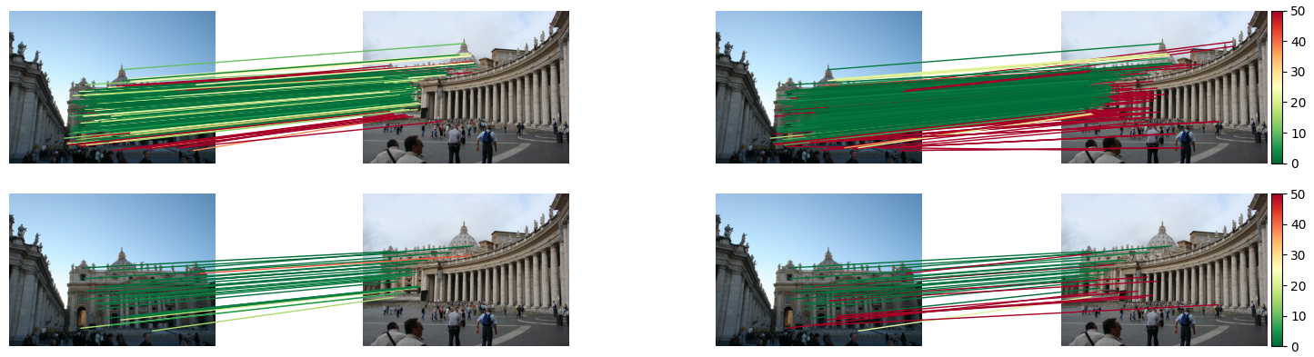
MA@2=62.3 MA${}_{\text{text}}$@2=81.1 errR=1.9’ errT=5.5’	MA@2=66.2 MA${}_{\text{text}}$@2=67.5 errR=2.1’ errT=9.4’
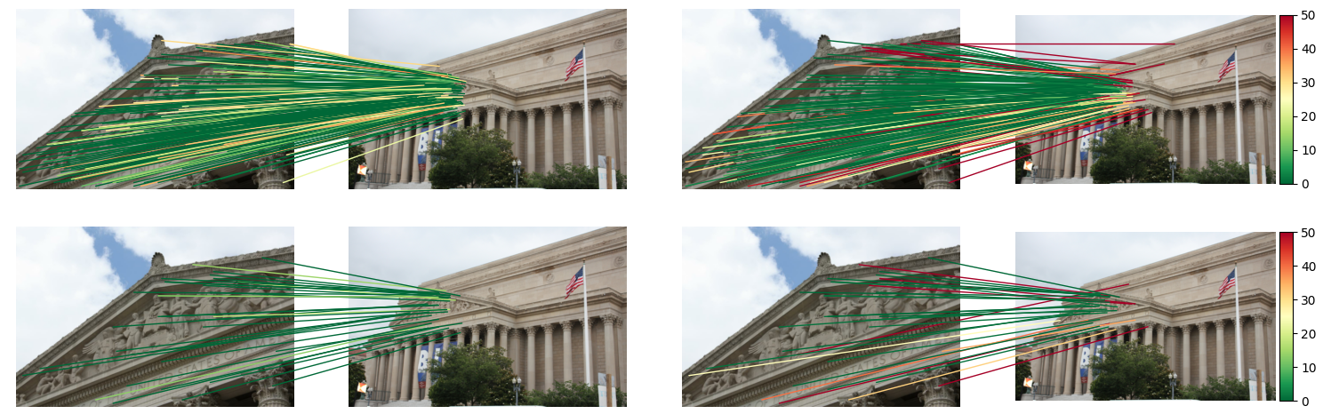
MA@2=79.0 MA${}_{\text{text}}$@2=83.1 errR=1.5’ errT=3.9’	MA@2=79.9 MA${}_{\text{text}}$@2=78.7 errR=2.0’ errT=6.4’
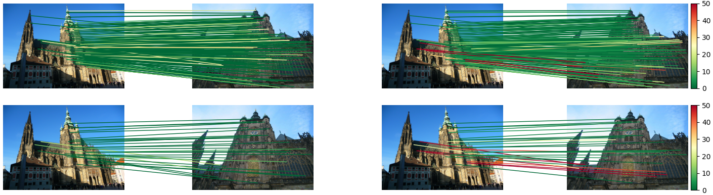
MA@5=69.1 MA${}_{\text{text}}$@5=78.0 errR=3.8’ errT=15.4’	MA@5=70.7 MA${}_{\text{text}}$@5=72.1 errR=4.9’ errT=19.6’

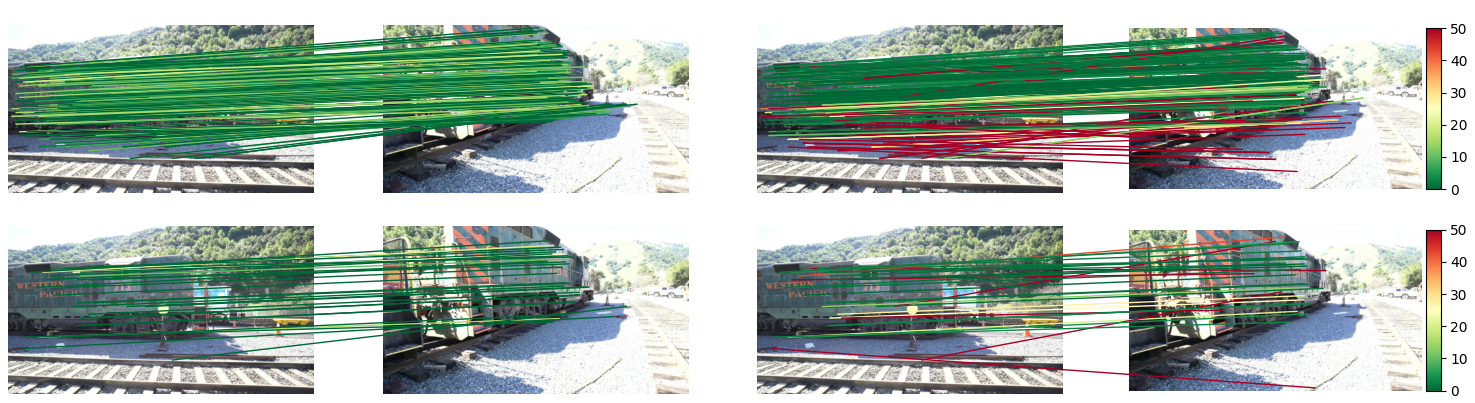
Figure 6: Qualitative results on MegaDepth1500. For each image pair: (top row) Visualization of established correspondences used to compute the MA, (bottom row) Visualization of established correspondences used to compute the MA${}_{\text{text}}$. Line colors indicate the distance in pixels with respect to the ground truth correspondent.

In Table 9, we propose an ablation study of SAM to evaluate the impact of each part of our architecture. This study is performed on MegaDepth validation scenes. Starting from a standard siamese CNN, we show that a significant gain in performance can simply be obtained with the input cross-attention layer (here the PE is added and not concatenated) and self-attention layers. We then add learned latent vectors (LV) in the latent space and use an output cross-attention which again significantly improves the performance. Concatenating the positional encoding information instead of adding it to the visual features reduces the matching accuracy at $\eta=2$ and $\eta=5$. However, combining it with structured attention leads to a significant improvement in terms of MA. Finally, as expected, the refinement step improves the matching accuracy for small pixel error thresholds.

In the supp. mat., we also provide a technical study showing that reducing the resolution from 1/4 to 1/8 significantly reduces the matching accuracy. On the contrary, augmenting the resolution from 1/4 to 1/2 only improves the matching accuracy for small values of $\eta$. This observation suggests that SDF methods, that process features with a resolution of 1/8, could significantly improve their ability to match local features by considering a resolution of 1/4.

Additional results are available in the supp. mat.

SAM (ours)	LoFTR+QuadTree [Tang et al., 2022]
MA@5=69.7 MA${}_{\text{text}}$@5=88.6 AUC@5=77.4	MA@5=72.1 MA${}_{\text{text}}$@5=76.6 AUC@5=76.1
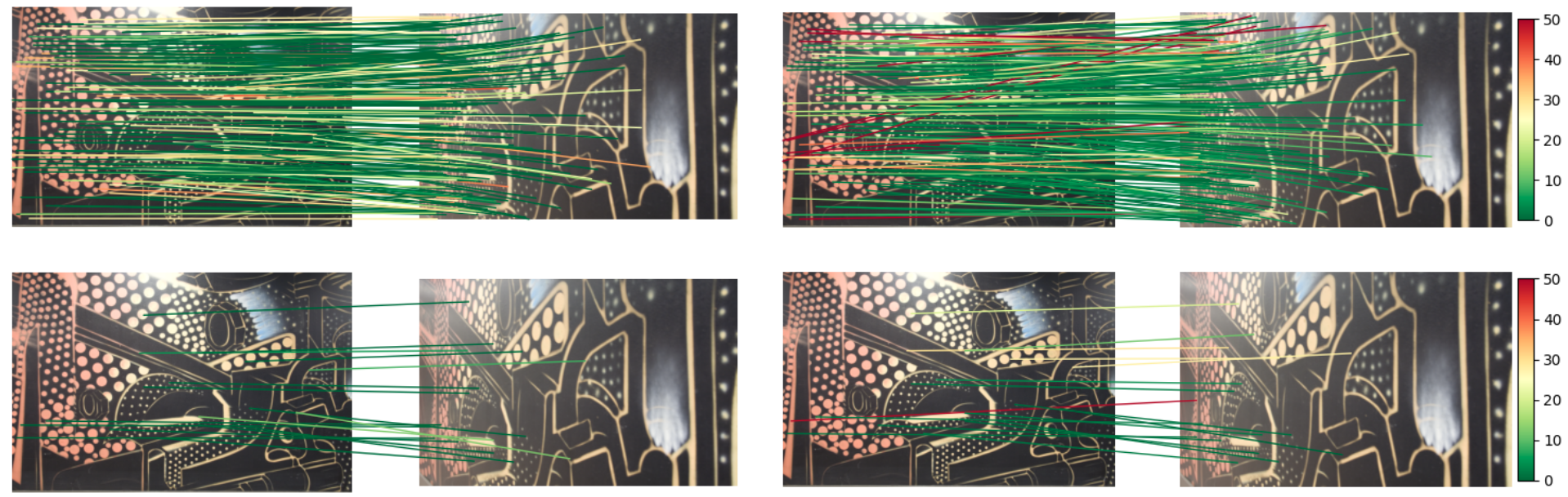
MA@5=74.4 MA${}_{\text{text}}$@5=86.2 AUC@5=81.5	MA@5=77.1 MA${}_{\text{text}}$@5=42.8 AUC@5=75.9

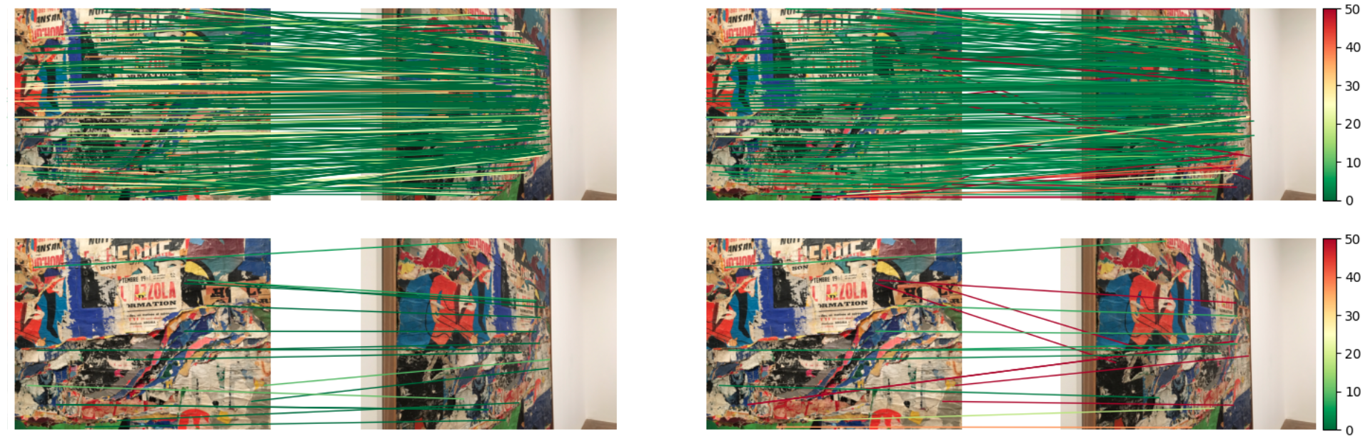
Figure 7: Qualitative results on HPatches. Line colors indicate the distance in pixels to the ground truth correspondent.

SAM (ours)	LoFTR+QuadTree [Tang et al., 2022]
MA${}_{\text{text}}$@2=75.0	MA${}_{\text{text}}$@2=68.8
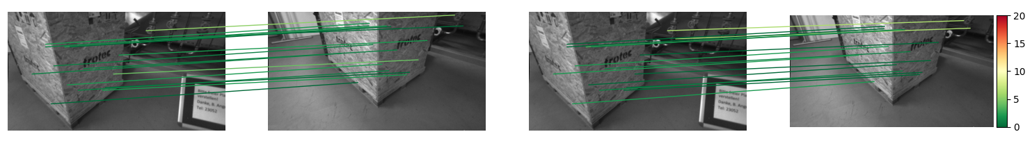
MA${}_{\text{text}}$@2=65.4	MA${}_{\text{text}}$@2=61.5
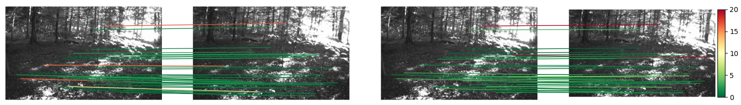
MA${}_{\text{text}}$@2=80.0	MA${}_{\text{text}}$@2=68.0
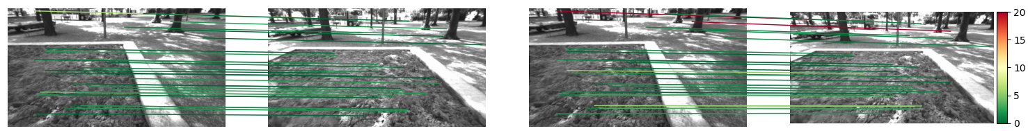
MA${}_{\text{text}}$@2=87.2	MA${}_{\text{text}}$@2=69.2

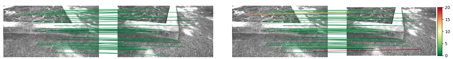
Figure 8: Qualitative results on ETH3D. Line colors indicate the distance in pixels to the ground truth correspondent.

SAM (ours)	LoFTR+QuadTree [Tang et al., 2022]
MA@2=60.6 MA${}_{\text{text}}$@2=84.0 errR=2.1’ errT=5.4’	MA@2=62.8 MA${}_{\text{text}}$@2=64.0 errR=5.5” errT=22.4’
MA@2=64.2 MA${}_{\text{text}}$@2=71.9 errR=5.4’ errT=4.3’	MA@2=68.8 MA${}_{\text{text}}$@2=69.5 errR=9.4’ errT=19.7’
MA@2=69.6 MA${}_{\text{text}}$@2=83.3 errR=1.5’ errT=1.4’	MA@2=70.2 MA${}_{\text{text}}$@2=75.8 errR=2.4’ errT=4.1’
MA@2=68.2 MA${}_{\text{text}}$@2=82.4 errR=2.4’ errT=9.5’	MA@2=73.3 MA${}_{\text{text}}$@2=76.5 errR=5.3’ errT=15.2’

Figure 9: Qualitative comparison of the ability to match local features: (left) SAM, (right) LoFTR+QuadTree [Tang et al., 2022] (line colors indicate the distance in pixels with respect to the ground truth correspondent).

In these experiments, we focus on evaluating the ability of six SDF networks (LoFTR [Sun et al., 2021], QuadTree [Tang et al., 2022], ASpanFormer [Chen et al., 2022], 3DG-STFM [Mao et al., 2022], MatchFormer [Wang et al., 2022], TopicFM [Giang et al., 2023]) and two FCO methods (COTR [jiang2021cotr] and ECO-TR [tan2022eco]) to match local features. We also evaluate SAM, our proposed architecture. In all the following Tables, best and second best results are respectively bold and underlined.

Implementations - For each network, we employ the code and weights (trained on MegaDepth) made available by the authors. Concerning SAM, we train it similarly to the aforementioned SDF and FCO networks on MegaDepth [Li and Snavely, 2018], during 100 hours, on four GeForce GTX 1080 Ti (11GB) GPUs (see supp. mat. for details).

Evaluation datasets - We consider three different widely used datasets to evaluate the ability of the methods to match local features: MegaDepth [Li and Snavely, 2018], HPatches [Balntas et al., 2017] and ETH3D [Schöps et al., 2019]. In order to fairly evaluate the different methods, we proceed as explained in Sec. 3.2 to obtain test sets. In particular, each method processes the same pairs of source/target images (with the same resolution) and is evaluated on the same 2D query locations. Our evaluation code and test sets will be made available.

Evaluation criteria - Given a test set $\mathcal{D_{\text{test}}}$ (see eq. 2), a method $\mathcal{M}$ to be evaluated first processes each sample of $\mathcal{D_{\text{test}}}$ (see eq. 3). For each prediction $\hat{\mathbf{p}}_{\text{t}_{k},i}$, the Euclidean distance $d_{k,i}$ with respect to the ground truth 2D location $\mathbf{p}_{\text{t}_{k},i}$ can be computed: $d_{k,i}=\left\lVert\hat{\mathbf{p}}_{\text{t}_{k},i}-\mathbf{p}_{\text{t}_{k},i}\right\rVert_{2}$. SDF methods are trained to detect or filter cases where the correspondent $\mathbf{p}_{\text{t}_{k},i}$ of $\mathbf{p}_{\text{s}_{k},i}$ is not covisible in the target image. Consequently, as evaluation criterion, we ignore predictions that are not tagged as visible ($\left[v_{\text{t}_{k},i}=0\right]$) and consider Matching Accuracies (MA) as in [Truong et al., 2020], the average on all images of the ratio of correct matches, for different pixel error thresholds ($\eta$):

$$\text{MA}\left(\eta\right)=\frac{1}{K}\sum_{k=1}^{K}\frac{\sum_{i=1}^{L_{k}}\left[v_{\text{t}_{k},i}=1\right]\left[d_{k,i}<\eta\right]}{\sum_{i=1}^{L_{k}}\left[v_{\text{t}_{k},i}=1\right]}.$$ (11)

RG: parler de MA${}_{\text{text}}$

RG: faire le lien avec PCK ?

Table 6: RG: Evaluation of the ability to match local features on MegaDepth1500 [Li and Snavely, 2018]. We report Matching Accuracy (11) for several thresholds $\eta$, computed on the set of all the semi-dense locations of the source image with available ground truth correspondent (MA), and on a subset containing only textured semi-dense locations (MA${}_{\text{text}}$), i.e., uniform regions are ignored. We also report the pose estimation accuracy. The proposed SAM method outperforms SDF methods in terms of pose estimation by establishing precise correspondences on textured regions while having a general lower accuracy.

Method	Matching Accuracy (MA) (11) $\uparrow$							Matching Accuracy							Pose estimation on
								on textured regions (MA${}_{\text{text}}$) (11) $\uparrow$							1/8 grid (AUC) $\uparrow$
	$\eta$=$1$	$\eta$=$2$	$\eta$=$3$	$\eta$=$5$	$\eta$=$10$	$\eta$=$20$		$\eta$=$1$	$\eta$=$2$	$\eta$=$3$	$\eta$=$5$	$\eta$=$10$	$\eta$=$20$		$@5^{\text{o}}$	$@10^{\text{o}}$	$@20^{\text{o}}$
LoFTR [Sun et al., 2021]	49.7	73.2	81.6	87.4	90.5	91.8		55.3	75.2	81.6	86.9	89.9	91.9		52.8	69.2	82.0
MatchFormer [Wang et al., 2022]	51.1	73.4	81.0	86.9	89.5	90.9		56.5	75.6	81.8	87.1	89.6	90.9		52.9	69.7	82.0
TopicFM [Giang et al., 2023]	51.4	75.4	83.7	89.9	92.9	93.5		59.8	77.6	84.8	90.4	92.9	93.7		54.1	70.1	81.6
3DG-STFM[Mao et al., 2022]	51.6	73.7	80.7	86.4	89.0	90.7		57.0	75.8	81.8	86.8	88.8	90.5		52.6	68.5	80.0
ASpanFormer [Chen et al., 2022]	52.0	76.2	84.5	90.7	93.7	94.8		62.2	80.3	85.9	91.0	93.7	94.7		55.3	71.5	83.1
LoFTR+QuadTree [Tang et al., 2022]	51.6	75.9	84.1	90.2	93.1	94.0		61.7	79.9	85.5	90.5	93.3	94.1		54.6	70.5	82.2
SAM (ours)	48.5	70.4	78.0	83.0	85.4	86.4		67.9	83.8	87.3	90.6	93.6	95.2		55.8	72.8	84.2

5.5 Evaluation on MegaDepth [Li and Snavely, 2018]

We consider MegaDepth validation scenes and create two different test sets: a mixed test set composed of 5000 pairs of images randomly sampled, and a hard test set of 1500 pairs exclusively sampled among pairs that display low visual overlaps. More details are provided in the supp. mat. We report in Tab. 6, RMSE and Matching Accuracy (eq. (11)) results for all the different methods. On both test sets, COTR significantly outperforms all the SDF methods in terms of matching accuracy. In terms of RMSE, COTR outperforms the SDF methods on the hard test set but is on par with them on the mixed test set, which indicates that all these methods exhibit a similar robustness. While ECO-TR and COTR have almost the same RMSE on both test sets, one can see that ECO-TR is significantly outperformed by COTR in terms of matching accuracy.

Concerning SAM, on both test sets, it is on par with COTR in terms of matching accuracy but significantly outperforms it in terms of RMSE, which suggest that SAM is more robust. SAM is also significantly faster than FCO architectures. In Figure 10, we qualitatively compare the ability of LoFTR+QuadTree and SAM to match local features on several image pairs.

Table 7: Evaluation of the ability to match local features on the ETH3D dataset [Schöps et al., 2019]. The results are reported for different frame interval sampling rates $r$. RG: preciser les tailles ? 640 RG: quelles colonnes on garde ? egalites de valeurs ?

Method	Matching Accuracy on textured regions (MA${}_{\text{text}}$) (11) $\uparrow$ ??? (ou on met ça dans la caption pour pas insister)
	$r=3$						$r=7$						$r=15$
	$\eta$=$1$	$\eta$=$2$	$\eta$=$3$	$\eta$=$5$	$\eta$=$10$		$\eta$=$1$	$\eta$=$2$	$\eta$=$3$	$\eta$=$5$	$\eta$=$10$		$\eta$=$1$	$\eta$=$2$	$\eta$=$3$	$\eta$=$5$	$\eta$=$10$
LoFTR [Sun et al., 2021]	44.8	76.5	88.4	97.0	99.4		39.7	73.1	87.6	95.9	98.5		33.3	66.2	84.8	92.5	96.3
MatchFormer [Wang et al., 2022]	45.5	77.1	89.2	97.2	99.7		40.4	73.8	87.8	96.6	99.0		34.2	66.7	84.9	93.5	97.0
TopicFM [Giang et al., 2023]	45.1	76.9	89.0	97.2	99.6		39.9	73.5	87.9	96.4	99.0		33.8	66.4	85.0	92.8	96.5
3DG-STFM[Mao et al., 2022]	43.9	76.3	88.0	96.9	99.3		39.3	72.7	87.4	95.5	98.3		32.4	65.7	84.7	92.0	96.0
ASpanFormer [Chen et al., 2022]	45.8	77.6	89.6	97.8	99.8		40.6	73.8	88.1	96.8	99.0		34.3	66.8	85.3	93.9	97.3
LoFTR+QuadTree [Tang et al., 2022]	45.9	77.5	89.5	97.8	99.7		40.8	74.0	88.3	97.0	99.2		34.5	66.8	85.4	94.0	97.3
SAM (ours)	53.4	79.9	91.5	98.0	99.8		48.6	78.6	91.7	98.2	99.4		40.1	70.2	87.8	95.4	97.8

5.6 Evaluation on ETH3D [Schöps et al., 2019]

We evaluate the different networks, trained on MegaDepth, on several sequences of the ETH3D dataset [Schöps et al., 2019] as proposed in [Truong et al., 2020]. Different frame interval sampling rates $r$ are considered. As the rate $r$ increases, the overlap between the image pairs reduces, hence making the matching problem more difficult. In Tab. 7, the RMSE obtained for each network is reported. All the methods obtain a low RMSE, which suggests that the image pairs are not very challenging. Nevertheless, one can see that ECO-TR outperforms all the SDF methods, while COTR surprisingly obtains among the worst results. SAM obtains either the best or second-best RMSE results for all rates.

Table 8: Evaluation of the ability to match local features on the HPatches dataset [Balntas et al., 2017]. RG: 2 soulignés en cas d’égalité ? Homography 5px

Method	Matching Accuracy				Matching Accuracy on				Homography estimation
	(MA) (11) $\uparrow$				textured regions (MA${}_{\text{text}}$) (11) $\uparrow$				(AUC) $\uparrow$
	$\eta$=$3$	$\eta$=$5$	$\eta$=$10$		$\eta$=$3$	$\eta$=$5$	$\eta$=$10$		$@3\text{px}$	$@5\text{px}$	$@10\text{px}$
LoFTR [Sun et al., 2021]	66.8	74.3	77.3		67.6	75.3	78.4		65.9	75.6	84.6
MatchFormer [Wang et al., 2022]	66.2	74.9	78.2		67.7	75.8	79.1		65.0	73.1	81.2
TopicFM [Giang et al., 2023]	72.7	85.0	87.5		74.0	86.0	88.5		67.3	77.0	85.7
3DG-STFM[Mao et al., 2022]	64.9	75.1	78.2		66.2	74.3	77.6		64.7	73.1	81.0
ASpanFormer [Chen et al., 2022]	76.2	86.2	88.7		73.9	85.8	88.4		67.4	76.9	85.6
LoFTR+QuadTree [Tang et al., 2022]	70.2	83.1	85.9		73.5	84.3	86.9		67.1	76.1	85.3
SAM (ours)	62.4	70.9	74.2		73.4	86.6	89.3		67.1	76.9	85.9

5.7 Evaluation on HPatches [Balntas et al., 2017]

We evaluate the different architectures on HPatches [Balntas et al., 2017]. The results are provided in Tab. 8. Again, FCO networks outperform all the SDF methods. COTR, ECO-TR and SAM obtain very similar performances for $\eta=5,10,20$. However, the simple refinement stage of SAM seems less efficient on this dataset as we can see that it is outperformed by COTR and ECO-TR for $\eta=1,2$. Nevertheless, SAM obtains the lowest RMSE.

5.8 Ablation study

Table 9: Ablation study of proposed SAM method (MegaDepth).

Method	Matching accuracy MA (11) $\uparrow$
	$\eta$=$1$	$\eta$=$2$	$\eta$=$5$	$\eta$=$10$	$\eta$=$20$	$\eta$=$50$
Siamese CNN	0.029	0.112	0.436	0.581	0.622	0.687
+ Input cross-attention (CA)	0.137	0.321	0.671	0.734	0.767	0.822
+ Self-attention (x16)	0.131	0.453	0.811	0.864	0.895	0.933
+ Learned LV and output CA	0.132	0.462	0.823	0.871	0.898	0.935
+ PE concatenated	0.121	0.419	0.796	0.868	0.902	0.939
+ Structured AM	0.140	0.487	0.857	0.902	0.922	0.947
+ Refinement (Full model)	0.673	0.791	0.870	0.902	0.921	0.946

In Tab. 9, we propose an ablation study of SAM to evaluate the impact of each contribution in our architecture. This study is performed are on MegaDepth validation scenes (see supp. mat for details). Starting from a standard siamese CNN, we show that a significant gain in performance can simply be obtained with the input cross-attention layer (here the PE is added and not concatenated). Then, the successive self-attentions are also useful by allowing the query vectors to communicate with each other.

We then add learned latent vectors (LV) in the latent space and use an output cross-attention which only slightly improves the performance.

Concatenating the positional encoding information instead of adding it to the visual features reduces the matching accuracy at $\eta=2$ and $\eta=5$. However, combining it with structured attention, leads to a significant improvement of the matching accuracy.

Finally, as expected, the refinement step improves the matching accuracy for small pixel error thresholds.

In the supp. mat., we also provide a technical study showing that reducing the resolution from 1/4 to 1/8 significantly reduces the matching accuracy. On the contrary, augmenting the resolution from 1/4 to 1/2 only improves the matching accuracy for small values of $\eta$. This observation suggests that SDF methods, that process features with a resolution of 1/8, could significantly improve their ability to match local features by considering a resolution of 1/4.

Additional results are available in the supp. mat.

SAM (ours)	LoFTR+QuadTree [Tang et al., 2022]
MA@2=60.6 MA${}_{\text{text}}$@2=84.0 errR=2.1’ errT=5.4’	MA@2=62.8 MA${}_{\text{text}}$@2=64.0 errR=5.5” errT=22.4’
MA@2=64.2 MA${}_{\text{text}}$@2=71.9 errR=5.4’ errT=4.3’	MA@2=68.8 MA${}_{\text{text}}$@2=69.5 errR=9.4’ errT=19.7’
MA@2=69.6 MA${}_{\text{text}}$@2=83.3 errR=1.5’ errT=1.4’	MA@2=70.2 MA${}_{\text{text}}$@2=75.8 errR=2.4’ errT=4.1’
MA@2=68.2 MA${}_{\text{text}}$@2=82.4 errR=2.4’ errT=9.5’	MA@2=73.3 MA${}_{\text{text}}$@2=76.5 errR=5.3’ errT=15.2’

Figure 10: Qualitative comparison of the ability to match local features: (left) SAM, (right) LoFTR+QuadTree [Tang et al., 2022] (line colors indicate the distance in pixels with respect to the ground truth correspondent).

6 Conclusion

We proposed a novel Structured Attention-based image Matching architecture (SAM). The flexibility of this novel architecture allowed us to fairly compare it against SDF methods, i.e., in all the experiments we used the same query locations (source grid with stride 8). The experiments highlighted a counter-intuitive result on two datasets (MegaDepth and HPatches): on the one hand SAM either outperforms or is on par with SDF methods in terms of pose/homography estimation metrics, but on the other hand SDF approaches are significantly better than SAM in terms of Matching Accuracy (MA). Here the MA is computed on all the semi-dense locations of the source image with available ground truth correspondent, which includes both textured and uniform regions. We proposed to limit the computation of the matching accuracy to textured regions, and showed that in this case SAM often surpasses SDF methods. These findings highlighted a strong correlation between the ability to establish precise correspondences in textured regions and the accuracy of the resulting estimated pose/homography. We also evaluated the aforementioned methods on ETH3D which confirmed, on a third dataset, that SAM has a strong ability to establish correspondences in textures regions. We finally performed an ablation study of SAM to demonstrate that each part of the architecture is important to obtain such a strong matching capacity.

APPENDIX

7 Extended related work

!!!!!!!!!!!!!! TODO TODO TODO !!!!!!!!!!!!!!!!!!!!!!

RG: Finally, note that very recent methods such as zhu2023pmatch, ni2023pats, yu2023adaptive or edstedt2023dkm have been proposed to perform dense matching.

RG: PMatch zhu2023pmatch (PMatch: Paired Masked Image Modeling for Dense Geometric Matching)
PATS ni2023pats (PATS: Patch area transportation with subdivision for local feature matching)
ASTR yu2023adaptive (Adaptive Spot-Guided Transformer for Consistent Local Feature Matching)
DKM edstedt2023dkm (Dense kernelized feature matching for geometry estimation) A functional correspondence model [jiang2021cotr, tan2022eco] takes as input a pair of source/target images, as well as a 2D query location in the source image, and predicts its 2D correspondent location in the target image. COTR [jiang2021cotr] was the first method to propose such a FCO model. Each image of the source/target image pair is first cropped and resized into a $256\!\times\!256\!\times\!3$ tensor and fed to a CNN backbone to obtain coarse features of size $16\!\times\!16\!\times\!256$. These coarse features are horizontally concatenated into a $16\!\times\!32\!\times\!256$ tensor and fed to a self-attention-based encoder. The output tensor of this encoder is fed to a cross-attention-based decoder using the 2D query location vector embedding (in the source image) as query. The resulting vector is finally decoded by an MLP into a 2D correspondent location in the target image. This 2D prediction is highly inaccurate, as the input features have a coarse resolution of 1/16. Therefore, the previously described functional network is recursively applied by zooming in on both images at the previously estimated correspondence locations. Although elegant, this functional approach makes the computational time of COTR unreasonable.

To reduce this run time, ECO-TR [tan2022eco] proposes a different functional correspondence architecture. They report performances that are on par with those of COTR while significantly reducing their computational time. Nevertheless, their run time remains excessively slow compared to SDF architectures.

8 Additional results

Matching accuracy curve.

In Fig. LABEL:fig:cumulative_fig, we report the matching accuracy curve for $\eta=1,2,...,49,50$ pix on the mixed MegaDepth test set. These results are an extended version of Tab. 2 in the main paper.

Performance/Inference time.

In Fig. LABEL:fig:efficiency_fig, we report the matching accuracy at distance thresholds $\eta=2$ and $\eta=50$ w.r.t. the inference time.

AEPE results.

In Tab. 7, we report the Average End Point Error (AEPE) results on the ETH3D dataset. This is the same experiment as Tab. 3 in the main paper except that we compute the AEPE instead of the RMSE.

Technical study

In Tab. 10, we provide a comparison of multiple SAM models trained to perform feature matching at 1/8, 1/4 and 1/2 of the original image resolution. We also include the results of a model using linear attention instead of softmax attention. The baseline model in this study corresponds to the fourth line in the Tab. 5 of the main paper, the SAM architecture with input cross-attention, self-attentions and learned latent vectors with output cross-attention. We observe that the matching resolution has a strong impact on the final matching accuracy. Matching at 1/8 reduces the overall accuracy compared to matching at 1/4. On the other hand matching at 1/2 improves the precision over the 1/4 model but does not bring any improvement in robustness. However, matching at 1/2 of the original resolution leads to significant increases in computational costs. Lastly, linear attention offers a noticeable drop in complexity, but yields much less accurate results than the original softmax attention.

These results suggest ADF methods, that process features with a resolution of 1/8, could significantly improve their ability to match local features by considering a resolution of 1/4.

Table 10: Technical study of proposed SAM method on MegaDepth validation scenes. We find that the 1/4 model provides the best compromise between performance and computational cost.

Method	Matching accuracy MA $\uparrow$
	$\eta$=$1$	$\eta$=$2$	$\eta$=$5$	$\eta$=$10$	$\eta$=$20$	$\eta$=$50$
SAM baseline 1/8	0.030	0.119	0.529	0.791	0.856	0.906
SAM baseline 1/4	0.132	0.462	0.823	0.871	0.898	0.935
SAM baseline 1/2	0.447	0.758	0.842	0.865	0.892	0.932
SAM bseline 1/4 linear attention	0.114	0.382	0.717	0.772	0.808	0.867

Structured attention discussion.

In Fig. 5 we propose a visualization of two different correspondence maps (before the ”output” cross-attention).

The first map is produced using the first 128 dimensions of the feature representation and contains high-level visio-positional features. The second map is produced using the 128 last dimensions of the feature representation and contains only positional encodings. By building these distinct correspondence maps we can observe that while the visio-spatial representation is sensitive to repetitive structures, the purely positional representation tends to be only activated in the areas neighbouring the match.

Learned latent space visualization.

In Fig. 4, we propose a visualization of the learned latent vectors of SAM. The average query map is obtained by averaging the 64 correspondence maps of the 64 query locations, while the average latent map is obtained by averaging the 128 correspondence maps of the 128 learned latent vectors. We observe that the average query map is mainly activated around the correspondents, whereas these regions are less activated in the average latent map.

SAM architecture.

Each attention layer in SAM is a classical series of softmax attention, normalization, MLP and normalization layers with residual connections, except for the ”output” cross-attention where we removed the MLP, the last normalization and the residual connection.

We empirically choose a combination of 16 self-attention layers and 128 vectors in the learned latent space. We found this combination to be a good trade-off between performance and computational cost.

Backbone description.

We use a modified ResNet-18 as our feature extraction backbone. We extract the feature map after the last ResBlock in which we removed the last ReLU. The features are reduced to ${\frac{1}{4}}^{th}$ of the image resolution ($3\times H\times W$) by applying a stride of 2 in the first and third layer. The feature representation built by the backbone is of size $128\times\frac{1}{4}H\times\frac{1}{4}W$.

Refinement description.

The previous CNN backbone is used for refinement. We simply added a FPN (Feature Pyramid Network) module to extract the feature maps after the first convolutional layer and each ResNet layer. It leaves us with a feature map of size $128\times H\times W$ on which the refinement stage is performed.

Structured attention.

In our implementation, $D=256$, we use 8 heads, thus $D_{H}=32$.

Training details.

The first part of the model to be trained is the refinement model (CNN+FPN). It is trained during 50 hours on 4 Nvidia GTX1080 Ti GPUs using Adam optimizer, a constant learning rate of $10^{-3}$ and a batch size of 1 (Figure 11). We minimize the cross-entropy of the full resolution correspondence maps produced using the FPN.

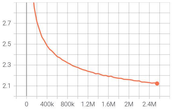
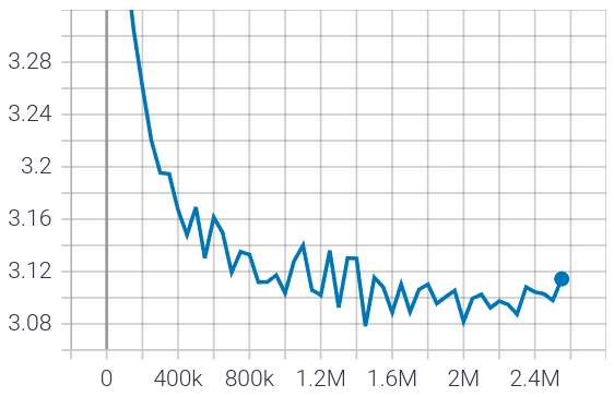
Figure 11: Training (left) and Validation (right) loss for refinement ResNet-18+FPN. x-axis represent the number of mini-batches seen by the model and y-axis the cross-entropy value.

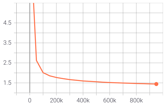
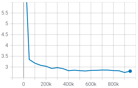
Figure 12: Training (left) and Validation (right) loss for SAM. x-axis represent the number of mini-batches seen by the model and y-axis the cross-entropy value.

The CNN backbone of SAM is initialized with the weights of the previously trained network. We train SAM for 100 hours. The same setup with 4 Nvidia GTX1080 Ti GPUs, Adam optimizer and a batch size of 1 is used. Concerning the learning rate schedule, we use a linear warm-up of 5000 steps (from $0$ to $10^{-4}$) and then an exponential decay (towards $10^{-5}$) (Figure 12). We minimize the cross-entropy of the $\frac{1}{4}$ resolution correspondence maps produced by SAM.

SAM (ours)	LoFTR+QuadTree [Tang et al., 2022]
MA@2=62.3 MA${}_{\text{text}}$@2=81.1 errR=1.9’ errT=5.5’	MA@2=66.2 MA${}_{\text{text}}$@2=67.5 errR=2.1’ errT=9.4’
MA@2=80.4 MA${}_{\text{text}}$@2=87.3 errR=1.1’ errT=4.2’	MA@2=82.6 MA${}_{\text{text}}$@2=83.1 errR=1.5’ errT=6.3’
MA@2=71.5 MA${}_{\text{text}}$@2=88.4 errR=2.1’ errT=2.7’	MA@2=78.2 MA${}_{\text{text}}$@2=83.8 errR=2.4’ errT=3.3’
MA@2=79.0 MA${}_{\text{text}}$@2=83.1 errR=1.5’ errT=3.9’	MA@2=79.9 MA${}_{\text{text}}$@2=78.7 errR=2.0’ errT=6.4’

Figure 13: Qualitative results on MegaDepth. For each image pair: (top row) Visualization of established correspondences used to compute the MA, (bottom row) Visualization of established correspondences used to compute the MA${}_{\text{text}}$. Line colors indicate the distance in pixels with respect to the ground truth correspondent.

SAM (ours)	LoFTR+QuadTree [Tang et al., 2022]
MA@5=81.7 MA${}_{\text{text}}$@5=85.9 errR=0.9’ errT=2.9’	MA@5=82.0 MA${}_{\text{text}}$@5=82.4 errR=1.8’ errT=3.4’
MA@5=73.4 MA${}_{\text{text}}$@5=83.9 errR=2.1’ errT=5.6’	MA@5=78.9 MA${}_{\text{text}}$@5=81.6 errR=2.6’ errT=6.8’
MA@5=69.1 MA${}_{\text{text}}$@5=78.0 errR=3.8’ errT=15.4’	MA@5=70.7 MA${}_{\text{text}}$@5=72.1 errR=4.9’ errT=19.6’
MA@5=78.8 MA${}_{\text{text}}$@5=83.1 errR=1.9’ errT=7.4’	MA@5=80.3 MA${}_{\text{text}}$@5=81.2 errR=2.2’ errT=8.0’

Figure 14: Qualitative results on MegaDepth. For each image pair: (top row) Visualization of established correspondences used to compute the MA, (bottom row) Visualization of established correspondences used to compute the MA${}_{\text{text}}$. Line colors indicate the distance in pixels to the ground truth correspondent.

9 Datasets details

For MegaDepth we use different splits for validation, training and testing. The splits are reported in Tab. 11.

Images are resized so that the largest dimension is equal to 640 pixels.

We created two test sets:
- a Mixed test set, by randomly sampling 5000 overlapping pairs of images within the test scenes.
- a Hard test set, by randomly sampling 1500 overlapping pairs of images within the test scenes, such that the overlap between two images is at most 20%.

On all benchmarks (MegaDepth, ETH3D and HPatches), for a fair comparison, for each pair of images, we randomly sampled (uniformly) the number $R$ of covisible correspondences between 1 and 32. This gave us $R$ query locations in the source image and $R$ ground truth correspondents in the target image. The remaining $64-R$ query locations in the source image were randomly sampled.

Table 11: MegaDepth scenes used for training, validation and test.

Training	Validation	Test
0, 1, 2, 3, 4, 5, 7, 8, 11, 12, 13, 15, 17, 19, 20, 21, 22, 23, 24, 25, 26, 27, 32, 35, 36, 37, 39, 42, 43, 46, 48, 50, 56, 57, 60, 61, 63, 65, 70, 80, 83, 86, 87, 95, 98, 100, 101, 103, 104, 105, 107, 115, 117, 122, 130, 137, 143, 147, 148, 149, 150, 156, 160, 176, 183, 189, 190, 200, 214, 224, 235, 237, 240, 243, 258, 265, 269, 299, 312, 326, 327, 331, 335, 341, 348, 366, 377, 380, 394, 407, 411, 430, 446, 455, 472, 474, 476, 478, 493, 494, 496, 505, 559, 733, 860, 1017, 1589, 4541, 5004, 5005, 5006, 5007, 5009, 5010, 5012, 5013, 5017	16, 33, 34, 41, 44, 47, 49, 58, 62, 64, 67, 71, 76, 78, 90, 94, 99, 102, 121, 129, 133, 141, 151, 162, 168, 175, 177, 178, 181, 185, 186, 197, 204, 205, 209, 212, 217, 223, 229, 231, 238, 252, 257, 271, 275, 277, 281, 285, 286, 290, 294, 303, 306, 307, 323, 349, 360, 387, 389, 402, 406, 412, 443, 482, 768, 1001, 3346, 5000, 5001, 5002, 5003, 5008, 5011, 5014, 5015, 5016, 5018	204, 252, 257, 271, 275, 277, 281, 285, 286, 290, 294, 303, 306, 307, 323, 349, 360, 387, 389, 402, 406, 412, 443, 482, 768, 1001, 3346, 5000, 5001, 5002, 5003, 5008, 5011, 5014, 5015, 5016, 5018

REFERENCES

- Arnold et al., 2022 Arnold, E., Wynn, J., Vicente, S., Garcia-Hernando, G., Monszpart, Á., Prisacariu, V. A., Turmukhambetov, D., and Brachmann, E. (2022). Map-free visual relocalization: Metric pose relative to a single image. In ECCV.
- Balntas et al., 2017 Balntas, V., Lenc, K., Vedaldi, A., and Mikolajczyk, K. (2017). Hpatches: A benchmark and evaluation of handcrafted and learned local descriptors. In CVPR.
- Chen et al., 2022 Chen, H., Luo, Z., Zhou, L., Tian, Y., Zhen, M., Fang, T., McKinnon, D., Tsin, Y., and Quan, L. (2022). Aspanformer: Detector-free image matching with adaptive span transformer. In ECCV.
- Dusmanu et al., 2019 Dusmanu, M., Rocco, I., Pajdla, T., Pollefeys, M., Sivic, J., Torii, A., and Sattler, T. (2019). D2-net: A trainable CNN for joint description and detection of local features. In CVPR.
- Edstedt et al., 2023 Edstedt, J., Athanasiadis, I., Wadenbäck, M., and Felsberg, M. (2023). Dkm: Dense kernelized feature matching for geometry estimation. In Proceedings of the IEEE/CVF Conference on Computer Vision and Pattern Recognition, pages 17765–17775.
- Germain et al., 2020 Germain, H., Bourmaud, G., and Lepetit, V. (2020). S2DNet: learning image features for accurate sparse-to-dense matching. In ECCV.
- Germain et al., 2021 Germain, H., Lepetit, V., and Bourmaud, G. (2021). Neural reprojection error: Merging feature learning and camera pose estimation. In CVPR.
- Germain et al., 2022 Germain, H., Lepetit, V., and Bourmaud, G. (2022). Visual correspondence hallucination. In ICLR.
- Giang et al., 2023 Giang, K. T., Song, S., and Jo, S. (2023). TopicFM: Robust and interpretable feature matching with topic-assisted. In AAAI.
- Heinly et al., 2015 Heinly, J., Schönberger, J. L., Dunn, E., and Frahm, J.-M. (2015). Reconstructing the World* in Six Days *(as Captured by the Yahoo 100 Million Image Dataset). In CVPR.
- Jaegle et al., 2022 Jaegle, A., Borgeaud, S., Alayrac, J.-B., Doersch, C., Ionescu, C., Ding, D., Koppula, S., Zoran, D., Brock, A., Shelhamer, E., Henaff, O. J., Botvinick, M., Zisserman, A., Vinyals, O., and Carreira, J. (2022). Perceiver IO: A general architecture for structured inputs & outputs. In ICLR.
- Jaegle et al., 2021 Jaegle, A., Gimeno, F., Brock, A., Vinyals, O., Zisserman, A., and Carreira, J. (2021). Perceiver: General perception with iterative attention. In ICML.
- Jin et al., 2020 Jin, Y., Mishkin, D., Mishchuk, A., Matas, J., Fua, P., Yi, K. M., and Trulls, E. (2020). Image Matching across Wide Baselines: From Paper to Practice. IJCV.
- Katharopoulos et al., 2020 Katharopoulos, A., Vyas, A., Pappas, N., and Fleuret, F. (2020). Transformers are RNNs: Fast autoregressive transformers with linear attention. In ICML.
- Li et al., 2020 Li, X., Han, K., Li, S., and Prisacariu, V. (2020). Dual-resolution correspondence networks. NeurIPS.
- Li and Snavely, 2018 Li, Z. and Snavely, N. (2018). Megadepth: Learning single-view depth prediction from internet photos. In CVPR.
- Lin et al., 2017 Lin, T.-Y., Dollár, P., Girshick, R., He, K., Hariharan, B., and Belongie, S. (2017). Feature pyramid networks for object detection. In CVPR.
- Lowe, 1999 Lowe, D. G. (1999). Object recognition from local scale-invariant features. In ICCV.
- Mao et al., 2022 Mao, R., Bai, C., An, Y., Zhu, F., and Lu, C. (2022). 3DG-STFM: 3D geometric guided student-teacher feature matching. In ECCV.
- Ni et al., 2023 Ni, J., Li, Y., Huang, Z., Li, H., Bao, H., Cui, Z., and Zhang, G. (2023). PATS: Patch area transportation with subdivision for local feature matching. In Proceedings of the IEEE/CVF Conference on Computer Vision and Pattern Recognition, pages 17776–17786.
- Ono et al., 2018 Ono, Y., Trulls, E., Fua, P., and Yi, K. M. (2018). LF-Net: learning local features from images. NeurIPS.
- Revaud et al., 2019 Revaud, J., De Souza, C., Humenberger, M., and Weinzaepfel, P. (2019). R2D2: reliable and repeatable detector and descriptor. NeurIPS.
- Rocco et al., 2020a Rocco, I., Arandjelović, R., and Sivic, J. (2020a). Efficient neighbourhood consensus networks via submanifold sparse convolutions. In ECCV.
- Rocco et al., 2018 Rocco, I., Cimpoi, M., Arandjelović, R., Torii, A., Pajdla, T., and Sivic, J. (2018). Neighbourhood consensus networks. NeurIPS.
- Rocco et al., 2020b Rocco, I., Cimpoi, M., Arandjelović, R., Torii, A., Pajdla, T., and Sivic, J. (2020b). NCNet: neighbourhood consensus networks for estimating image correspondences. PAMI.
- Sarlin et al., 2020 Sarlin, P.-E., DeTone, D., Malisiewicz, T., and Rabinovich, A. (2020). Superglue: Learning feature matching with graph neural networks. In CVPR.
- Sarlin et al., 2022 Sarlin, P.-E., Dusmanu, M., Schönberger, J. L., Speciale, P., Gruber, L., Larsson, V., Miksik, O., and Pollefeys, M. (2022). LaMAR: Benchmarking Localization and Mapping for Augmented Reality. In ECCV.
- Sattler et al., 2017 Sattler, T., Torii, A., Sivic, J., Pollefeys, M., Taira, H., Okutomi, M., and Pajdla, T. (2017). Are large-scale 3D models really necessary for accurate visual localization? In CVPR.
- Schönberger and Frahm, 2016 Schönberger, J. L. and Frahm, J.-M. (2016). Structure-from-motion revisited. In CVPR.
- Schöps et al., 2019 Schöps, T., Sattler, T., and Pollefeys, M. (2019). BAD SLAM: Bundle adjusted direct RGB-D SLAM. In CVPR.
- Strasdat et al., 2011 Strasdat, H., Davison, A. J., Montiel, J. M., and Konolige, K. (2011). Double window optimisation for constant time visual slam. In ICCV.
- Sun et al., 2021 Sun, J., Shen, Z., Wang, Y., Bao, H., and Zhou, X. (2021). LoFTR: detector-free local feature matching with transformers. In CVPR.
- Svärm et al., 2017 Svärm, L., Enqvist, O., Kahl, F., and Oskarsson, M. (2017). City-scale localization for cameras with known vertical direction. PAMI.
- Taira et al., 2018 Taira, H., Okutomi, M., Sattler, T., Cimpoi, M., Pollefeys, M., Sivic, J., Pajdla, T., and Torii, A. (2018). InLoc: Indoor visual localization with dense matching and view synthesis. In CVPR.
- Tang et al., 2022 Tang, S., Zhang, J., Zhu, S., and Tan, P. (2022). Quadtree attention for vision transformers. In ICLR.
- Truong et al., 2020 Truong, P., Danelljan, M., and Timofte, R. (2020). Glu-net: Global-local universal network for dense flow and correspondences. In CVPR.
- Truong et al., 2021 Truong, P., Danelljan, M., Van Gool, L., and Timofte, R. (2021). Learning accurate dense correspondences and when to trust them. In CVPR.
- Vaswani et al., 2017 Vaswani, A., Shazeer, N., Parmar, N., Uszkoreit, J., Jones, L., Gomez, A. N., Kaiser, Ł., and Polosukhin, I. (2017). Attention is all you need. NeurIPS.
- Wang et al., 2022 Wang, Q., Zhang, J., Yang, K., Peng, K., and Stiefelhagen, R. (2022). Matchformer: Interleaving attention in transformers for feature matching. In ACCV.
- Wang et al., 2021 Wang, W., Xie, E., Li, X., Fan, D.-P., Song, K., Liang, D., Lu, T., Luo, P., and Shao, L. (2021). Pyramid vision transformer: A versatile backbone for dense prediction without convolutions. In ICCV.
- Xie et al., 2021 Xie, E., Wang, W., Yu, Z., Anandkumar, A., Alvarez, J. M., and Luo, P. (2021). Segformer: Simple and efficient design for semantic segmentation with transformers. NeurIPS.
- Yi et al., 2016 Yi, K. M., Trulls, E., Lepetit, V., and Fua, P. (2016). LIFT: Learned invariant feature transform. In ECCV.
- Zhang et al., 2021 Zhang, Z., Sattler, T., and Scaramuzza, D. (2021). Reference pose generation for long-term visual localization via learned features and view synthesis. IJCV.
- Zhou et al., 2021 Zhou, Q., Sattler, T., and Leal-Taixe, L. (2021). Patch2Pix: Epipolar-guided pixel-level correspondences. In CVPR.
- Zhu and Liu, 2023 Zhu, S. and Liu, X. (2023). Pmatch: Paired masked image modeling for dense geometric matching. In Proceedings of the IEEE/CVF Conference on Computer Vision and Pattern Recognition, pages 21909–21918.