Finite density QCD equation of state: critical point and lattice-based $T^{\prime}$-expansion

Abstract

We present a novel construction of the QCD equation of state (EoS) at finite baryon density. Our work combines a recently proposed resummation scheme for lattice QCD results with the universal critical behavior at the QCD critical point. This allows us to obtain a family of equations of state in the range $0\leq\mu_{B}\leq 700$ MeV and 25 MeV $\leq T\leq 800$ MeV, which match lattice QCD results near $\mu_{B}=0$ while featuring a critical point in the 3D Ising model universality class. The position of the critical point can be chosen within the range accessible to beam-energy scan heavy-ion collision experiments. The strength of the singularity and the shape of the critical region are parameterized using a standard parameter set. We impose stability and causality constraints and discuss the available ranges of critical point parameter choices, finding that they extend beyond earlier parametric QCD EoS proposals. We present thermodynamic observables, including baryon density, pressure, entropy density, energy density, baryon susceptibility and speed of sound, that cover a wide range in the QCD phase diagram relevant for experimental exploration.

I Introduction

The determination of the multi-dimensional QCD phase diagram is one of the main ingredients in understanding matter under extreme conditions of temperature and density, such as those created in heavy-ion collision experiments taking place at the Relativistic Heavy Ion Collider (RHIC) and the Large Hadron Collider (LHC). In nature, this kind of matter could be present in the core of neutron stars, and also in a primordial phase that permeated the universe a few microseconds after the Big Bang. To determine the QCD phase diagram we need to explore the thermodynamic behavior of strongly interacting matter, including its phase structure, equation of state (EoS) and critical phenomena [1].

In its most common representation [2, 3], which involves temperature and baryon chemical potential or baryon density, the EoS at low net-baryon density is well understood. It exhibits a smooth crossover from a hadron gas to a quark-gluon plasma [4, 5, 6, 7, 8] with a pseudo-critical temperature of $T_{0}=158.0\pm 0.6$ MeV [9], and can be determined from first principles through lattice QCD simulations [5, 10, 11, 12, 13, 14, 15]. Several QCD models predict that the smooth crossover can turn into a first-order phase transition at high densities, thus implying the existence of a critical point on the QCD phase diagram [16, 17, 18, 19]. The search for the critical point is at the core of the Beam Energy Scan II (BESII) at RHIC, which completed data taking recently. The role of theorists in this program is to provide crucial tools to simulate and interpret the data. The equation of state is one of the fundamental quantities needed in the hydrodynamic description of the heavy-ion collision evolution.

Lattice simulations at finite chemical potential face challenges because of the fermion sign problem [20, 21, 22, 23], which renders traditional numerical techniques prohibitively costly. Despite recent developments in methods to directly simulate at finite chemical potentials, such as reweighting [24, 25, 26], these are still limited to small volumes and rather coarse lattices. This has so far prevented realistic direct simulations in the most intriguing region of the QCD phase diagram. Therefore, the expected first-order phase transition from hadron gas to quark-gluon plasma at high density, as well as the critical point terminating this transition [18, 1] are still out of the reach of lattice simulations. Extrapolation techniques, such as Taylor expansion [27, 28, 29, 30, 31, 32, 8, 33], analytic continuation from imaginary chemical potential [34, 35, 36, 37, 6, 38, 39, 12, 9] and Padé approximation [40, 15], are usually employed to extend lattice QCD thermodynamic results to finite densities. However, they are limited in their applicability to small chemical potentials.

An important tool for the theoretical interpretation of experimental results are hydrodynamic simulations

[41, 42, 43, 44, 45, 46, 47, 48], which describe the evolution of the fireball produced in heavy-ion collisions. Although modifications to the relativistic viscous hydrodynamic approach are required close to the critical point [41, 49], it is crucial that the equation of state (EoS) used in these simulations encompasses all existing theoretical knowledge and accurately represents the singularity related to the QCD critical point in a predetermined and adjustable way. Moreover, the EoS as well as the properties of partons and their interactions are probed directly within microscopic transport approaches, wherein partonic and hadronic degrees of freedom are propagated explicitly [50].

In an attempt to provide a tool to address these issues, the BEST collaboration developed a family of equations of state, based on the lattice QCD Taylor expansion, with a 3D Ising model critical point which matches lattice results at low chemical potential [51, 52, 53, 54]. However, this approach is limited to $\mu_{B}\leq 450$ MeV, because unphysical oscillation inherited from the Taylor expansion appear in some observables at large $\mu_{B}$ [55, 51].

It is important to note that the temperature of the hypothetical chiral critical point should not exceed the critical temperature of the chiral phase transition (for $m_{u}=m_{d}=0$) $T^{0}_{c}=132^{+3}_{-6}$ MeV [56, 57]. Lattice QCD simulations disfavor the existence of the critical point at $\mu_{B}\leq 300$ MeV [9]. Besides, several recent results seem to converge in predicting a critical point location at $560\leq\mu_{B}\leq 650$ MeV [58, 59, 60, 61, 62]. For this reason, and to properly support the BESII at RHIC that can cover a range up to $\mu_{B}\lesssim 700$ MeV, the BEST collaboration EoS needs to be extended to larger values of $\mu_{B}$. While some results exist in the literature [63], where a critical scaling function was developed on top of an EoS with a smooth crossover between hadrons and quarks, here we follow the same strategy as the BEST collaboration EoS: we introduce the 3D Ising critical point into a lattice-QCD-based EoS. However, instead of using the Taylor expansion method, we build our EoS on the basis of the new expansion scheme developed in [13, 14]. This will allow us to reach a value of chemical potential $\mu_{B}\sim 700$ MeV.

The manuscript is organized as follows. In section II we recall the lattice QCD approaches: Taylor expansion and alternative $T$-expansion scheme developed by the Wuppertal-Budapest lattice QCD collaboration in [13, 14]. Section III focuses on the mapping of the 3D Ising model onto the QCD coordinates. Moving on to section IV, we discuss the merging of the lattice QCD equation of state with the critical one. In section V, we present the thermodynamic quantities with a critical point, and in section VI we explore the constraints on the parameter space. Conclusions and outlook will be provided in section VII. Finally, in Appendix A,B and C we provide detailed derivation for the formulas used. The code that generates the family of equations of state presented in this paper can be downloaded from [64].

II Lattice Equation of State

II.1 Taylor Expansion

Taylor expansion is the most straightforward way to extend the equation of state to finite $\mu_{B}$. It consists of a sum of all pressure derivatives (susceptibilities), computed on the lattice at $\mu_{B}=0$, multiplied by powers of a dimensionless expansion parameter $\left(\frac{\mu_{B}}{T}\right)$. Because of charge conjugation symmetry, only even susceptibilities contribute

$$\frac{P(T,\mu_{B})}{T^{4}}=\sum_{n=0}{\frac{1}{2n!}\chi_{2n}(T,\mu_{B}=0)\left(\frac{\mu_{B}}{T}\right)^{2n}}\,\,,$$ (1)

where the coefficients are:

$$\chi_{n}(T)=\left(\frac{\partial^{n}}{\partial(\mu_{B}/T)^{n}}\frac{P(T,\mu_{B})}{T^{4}}\right)_{\mu_{B}=0}\,\,.$$

In this paper, we will focus on the baryon density, which is defined as the first derivative of the pressure with respect to $\mu_{B}$:

$$\frac{n_{B}(T,\mu_{B})}{T^{3}} = \frac{\partial}{\partial(\mu_{B}/T)}\frac{P(T,\mu_{B})}{T^{4}}$$ (2)

$$= \sum_{n=1}^{\infty}\frac{1}{(2n-1)!}\chi_{2n}(T)\left(\frac{\mu_{B}}{T}\right)^{2n-1}.$$

To completely evaluate the baryon density in Eq. (2), we would need all the coefficients computed on the lattice, which are not readily available due to limitations in computational power. Currently, coefficients are available at finite lattice spacing up to order $\mathcal{O}\left(\frac{\mu_{B}}{T}\right)^{6}$ [65, 66] and even $\mathcal{O}\left(\frac{\mu_{B}}{T}\right)^{8}$ [12, 15], and in the continuum limit in a smaller volume [67], which leads to the following limitations of the method:

• The chemical potential range is limited to $\frac{\mu_{B}}{T}<3$, despite large computational power [40, 15].

• At large $\mu_{B}/T$, some observables exhibit unphysical, “wiggly” behavior due to the truncation of the Taylor series [55, 51].

• The inclusion of an additional higher-order term does not improve this behavior.

• The Taylor expansion struggles to account for a transition temperature that depends on the chemical potential, since it is performed at constant temperature. In [68], the Taylor expansion was tested for finite isospin chemical potential by comparing it to the direct lattice simulation, and a breakdown was observed at the critical chemical potential.

The above limitations make it difficult to model and constrain the existence of the critical point if it is located at high density. In [51, 52, 53, 54], the BEST collaboration exploited the universality class of the 3D Ising model to introduce a critical point into the equation of state by separating the free energy density into a critical contribution and a non-critical one, so that the sum of the Taylor expansion coefficients up to $\mathcal{O}((\mu_{B}/T)^{4})$ reproduces the lattice results. For the baryon density, this procedure works as follows

$$n_{B}(T,\mu_{B}) =T^{3}\sum_{n=1}^{2}\frac{1}{(2n-1)!}\chi_{2n}^{\rm non-Ising}(T)\left(\frac{\mu_{B}}{T}\right)^{2n-1}$$

$$~{}~{}~{}~{}~{}~{}~{}~{}~{}~{}~{}~{}~{}~{}~{}~{}~{}~{}~{}~{}~{}~{}~{}~{}~{}~{}~{}~{}+\frac{T_{C}^{4}}{T}n_{B}^{\rm Ising}(T,\mu_{B})$$ (3)

where $n_{B}^{\rm Ising}$ is the contribution to the baryon density with the singular behavior appropriate for the 3D Ising critical point, and the coefficients $\chi_{n}^{\rm non-Ising}(T)$ satisfy

$$\chi_{n}^{\rm lat}(T)=\chi_{n}^{\rm non-Ising}(T)+\frac{T_{C}^{4}}{T^{4}}\chi_{n}^{\rm Ising}(T)$$

for $n=0,~{}2,~{}4$, where $\chi_{n}^{\rm lat}(T)$ are the input from lattice QCD and $\chi_{n}^{\rm Ising}(T)$ represent the critical contribution to the expansion coefficients. Although this construction works well, it was observed that at large values of $\mu_{B}$, wiggles appear in the thermodynamic observables, particularly the baryon density and speed of sound, for some parameter choices. This is due to the truncation in the Taylor expansion of the non-Ising contribution to the observables, which limits the current applicability of this equation of state.

II.2 $T^{\prime}$-Expansion Scheme

To address some of the limitations of the Taylor expansion outlined above, the Wuppertal-Budapest lattice QCD collaboration developed a novel resummation scheme, which can reach higher values of chemical potential and handle the QCD transition line [13, 14]. The scheme is based on the observation [13] that the crossover in terms of the scaled baryon density $T\chi_{1}^{B}/\mu_{B}$ as a function of $T$ looks very similar at different (imaginary) values of scaled chemical potential $\mu_{B}/T$, with most of the difference being a $\mu_{B}$-dependent shift of $T$ – see Fig.1.

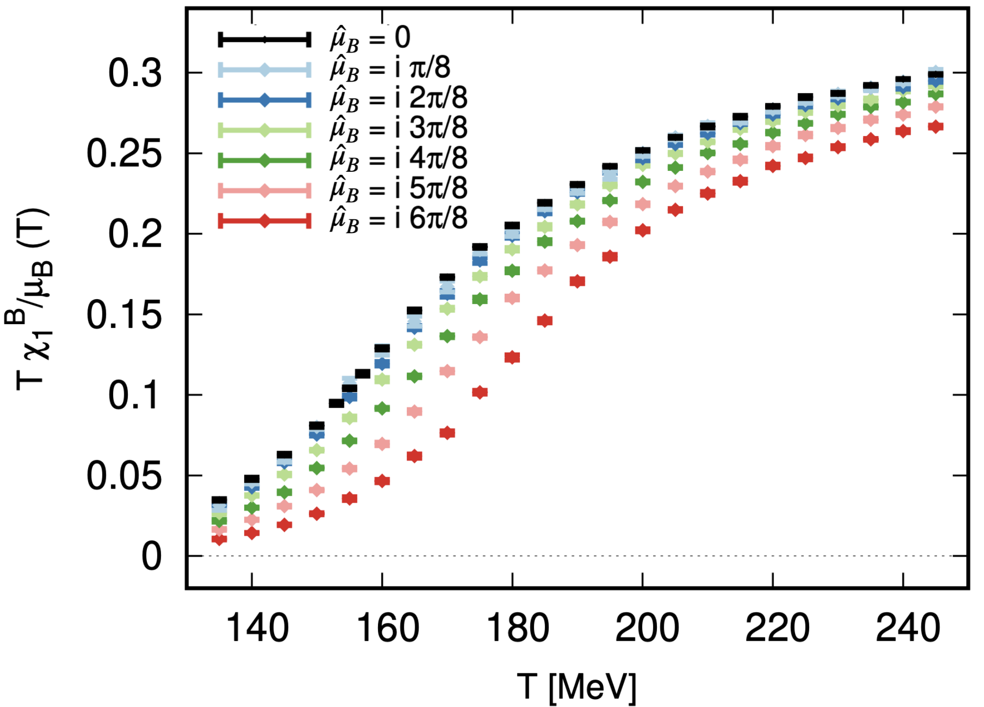
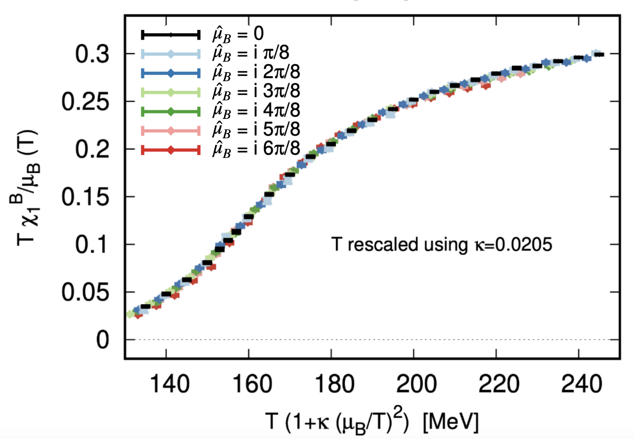
Figure 1: Upper panel: scaled baryon density ${\chi_{1}^{B}(T,\mu_{B})}/{\hat{\mu}_{B}}$, as a function of temperature for different values of scaled imaginary baryon chemical potential $\hat{\mu}_{B}\equiv{\mu_{B}}/{T}$ (labeled using different colors). Lower panel: the same quantity, but with the temperature rescaled by a factor $1+\kappa\hat{\mu}_{B}^{2}$, with $\kappa=0.0205$. In terms of the rescaled temperature the curves representing different $\hat{\mu}_{B}$ collapse onto the same curve. The points labeled $\hat{\mu}_{B}=0$ correspond to the limit $\mu_{B}\to 0$ which is the baryon number susceptibility $\chi^{B}_{2}(T,0)$ (The figure is taken from Ref. [13]).

This observation can be formalized by expressing baryon density $n_{B}\equiv\chi_{1}^{B}T^{3}$ in the form

$$T\frac{\chi_{1}^{B}(T,\mu_{B})}{\mu_{B}}=\chi_{2}^{B}(T^{\prime},0)$$ (4)

which defines the “rescaled temperature” $T^{\prime}(T,\mu_{B})$. At $\mu_{B}=0$, $T^{\prime}$ is the same as $T$. At non-zero $\mu_{B}$ function $T^{\prime}(T,\mu_{B})$ is such that the crossover in terms of $T{\chi_{1}^{B}(T,\mu_{B})}/{\mu_{B}}$ occurs at the same $T^{\prime}$ and has the same shape. The function $T^{\prime}$ can be then expanded in powers of $\mu_{B}/T$ at fixed $T$:

$$T^{\prime}(T,\mu_{B})=T\left[1+\kappa_{2}^{BB}(T)\left(\frac{\mu_{B}}{T}\right)^{2}+\kappa_{4}^{BB}(T)\left(\frac{\mu_{B}}{T}\right)^{4}+...\right]\,$$ (5)

where the Taylor expansion coefficients $\kappa_{2}^{BB}$, etc. are almost constant as functions of $T$ in the transition region, while the rapid changes in EoS associated with the crossover are mostly captured by the function $\chi_{2}(T^{\prime},0)$ (see Fig.2 below.).

The “$T^{\prime}$-expansion” scheme is essentially a re-shuffling of the Taylor expansion in Eq.(2), and the coefficients $\kappa_{n}^{BB}(T)$ can be expressed in terms of the susceptibilities $\chi_{2n}(T)$:

$$\kappa_{2}^{BB}(T) =\frac{1}{6T}\frac{\chi_{4}^{B}(T)}{{\chi_{2}^{B}}^{\prime}(T)}$$ (6)

$$\kappa_{4}^{BB}(T) =\frac{1}{130T{\chi_{2}^{B}}^{\prime}(T)^{3}}\left(3{\chi_{2}^{B}}^{\prime}(T)^{2}\chi_{6}^{B}(T)-5{\chi_{5}^{B}}^{\prime\prime}\chi_{4}^{B}(T)^{4}\right).$$

These coefficients were obtained in high-statistics lattice QCD simulations [13]. As expected, compared to the sharply rising $\chi_{2}^{B}(T)$, $\kappa_{2}^{BB}$ shows a very mild temperature dependence around the transition region, which makes the $T^{\prime}$-expansion scheme more favorable than the Taylor expansion since it does not introduce the wiggly behavior in the EoS at large $\mu_{B}$. Moreover, the fact that $\kappa_{4}$ is shown in [13] to be consistent with zero hints at a faster convergence compared to the Taylor series.

These results agree with the one used in [32] for “lines of constant physics” calculated up to $\mathcal{O}(\mu_{B}^{4})$. As suggested in [13], as long as $\chi_{1}^{B}/\hat{\mu}_{B}$ is a monotonic function of $T$, the finite-density physics can be encoded into the $T^{\prime}(T,\mu_{B})$ function. As a result, we can embed the singularity associated with the critical point and the first-order phase transition into $T^{\prime}(T,\mu_{B})$, as we will show in Section IV.

II.3 Lattice data

Lattice results for the susceptibility $\chi_{2}^{B}(T,0)\equiv\chi_{2}^{B}(T)$ and coefficients $\kappa_{2}^{BB}(T)$ are available only over a limited range of (discrete) temperatures. To obtain a smooth description of the equation of state in the temperature range $25\,\text{MeV}\leq T\leq 800$ MeV, we first merge the lattice results at finite temperature and $\mu_{B}=0$ with 2+1 flavors and physical quark masses from the Wuppertal-Budapest Collaboration [5, 10, 30, 12] with the hadron resonance gas (HRG) model results [69], which provide a good description of the thermodynamics up to $T=120$ MeV, using the most up to date particle list (list PDG2021+) [70, 71]. We then fit these results to cover a large range of temperatures.

For convenience we introduce an auxiliary variable $x=\frac{T}{200\,\text{MeV}}$. For $\chi_{2,\text{lat}}^{B}(T)$, we employ four free parameters $d_{i}$, such that the crossover occurs at $x\approx d_{1}$, and its width $\Delta x\sim d_{1}/d_{2}$ is controlled by $d_{2}\gg 1$, while $d_{3}\left(1-\frac{d_{4}^{2}}{x^{2}}\right)$ provides large-$x$ asymptotics:

$$\chi_{2,\rm lat}^{B}(T)=\left(\frac{2m_{p}}{\pi x}\right)^{3/2}\frac{e^{-m_{p}/x}}{1+\left(\frac{x}{d_{1}}\right)^{d_{2}}}+d_{3}\frac{e^{-d_{4}^{2}/x^{2}-d_{5}^{4}/x^{4}}}{1+\left(\frac{x}{d_{1}}\right)^{-d_{2}}}$$ (7)

where, $m_{p}$ denotes the proton mass (in units of 200 MeV), and the first term, typically very small, yields the correct low-temperature asymptotics for $\chi_{2}^{B}$ in QCD, representing the nonrelativistic contribution of nucleons/antinucleons. Best-fit coefficients for $\chi_{2,\text{lat}}^{B}(T)$ are listed in Table 1, and the resulting parametrization is shown in the top panel of Fig. 2.

$d_{1}$	$d_{2}$	$d_{3}$	$d_{4}$	$d_{5}$
$0.73$	$11.19$	$0.32$	$0.20$	$0.69$

Table 1: Coefficients of the parameterized $\chi_{2,\text{lat}}^{B}(T)$ in Eq. (7) for $25~{}\text{MeV}\leq T\leq 800~{}\text{MeV}$

For $\kappa_{2}^{BB}$, we employ a rational fit, enforcing the expected small-$x$ linear behaviour and the large-$x$ $\kappa_{2}^{BB}\sim A\,x^{2}$ dependence, with $A=\chi_{4,\rm SB}^{B}/(12d_{3}d_{4}^{2})$, where $\chi_{4,\rm SB}^{B}$ is the fourth baryon susceptibility in the infinite-temperature limit.

$$\kappa_{2}^{BB}(T)=\frac{a_{1}x+a_{2}x^{2}+a_{3}x^{3}+a_{4}x^{4}+a_{5}x^{5}}{b_{0}+b_{1}x+b_{2}x^{2}+a_{5}/A\,x^{3}}$$ (8)

and again $x=\frac{T}{200\,\rm MeV}$. Best-fit parameters for $\kappa_{2}^{BB}(T)$ are listed in Table 2, and the resulting parametrization is shown in the bottom panel of Fig. 2.

$a_{1}$	$a_{2}$	$a_{3}$	$a_{4}$	$a_{5}$	$b_{0}$	$b_{1}$	$b_{2}$	$b_{3}$
0.48	-0.64	0.52	-0.78	0.53	11.9	-9.62	-7.51	10.8

Table 2: Coefficients of the parameterized form for $\kappa^{B}_{2}(T)$ from Eq (8) for $25~{}\text{MeV}\leq T\leq 800~{}\text{MeV}$ given as a ratio.

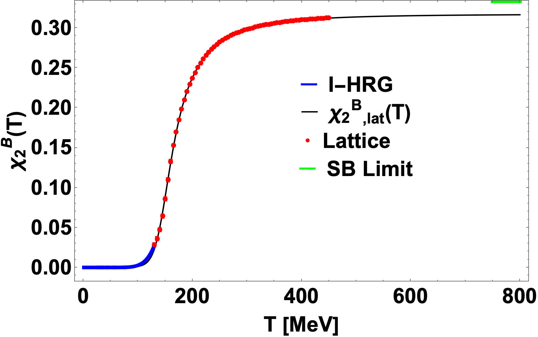
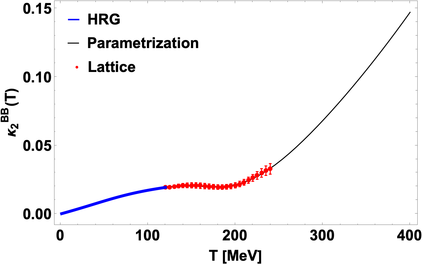
Figure 2: Top panel: parameterized baryon susceptibility $\chi^{B}_{2,\rm lat}(T)$ (black curve), in the range $25\,\text{MeV}<T<800\text{MeV}$. The Stefan-Boltzmann (SB) limit value is shown in green. Bottom panel: parametrized alternative expansion coefficient as a function of the temperature. In both panels, the solid blue curve corresponds to the hadron resonance gas (HRG) model prediction, while the red dots represent continuum extrapolated lattice QCD results.

III Mapping the 3D Ising model to QCD

Close to the critical point, the correlation length of a thermodynamic system diverges, making microscopic (short-distance) features irrelevant. Consequently, systems with similar global symmetries exhibit similar, universal behavior, even though they may differ in their microscopic degrees of freedom. Well-known examples of this phenomenon include liquid-gas and ferromagnetism, which share critical exponents within the same universality class as the 3D Ising model [72, 73]. The critical point of Quantum Chromodynamics (QCD), if it exists, also belongs to the 3D Ising model universality class [74]. Hence, its critical behavior is characterized by the same critical exponents, which describe the scaling of physical quantities in the thermodynamic variables near the critical point [74].

III.1 Scaling: 3D Ising Model

In this work, we employ the same form of the scaling equation of state as used in the BEST collaboration equation of state. The parameterization of magnetization, denoted by $M$, reduced temperature ($r$) and external magnetic field ($h$) in terms of additional scaling variables $R$ and $\theta$, is given as follows [51, 75, 76, 77, 78, 79, 80]:

$$M=~{} M_{0}R^{\beta}\theta$$ (9)

$$h=~{} h_{0}R^{\beta\delta}\tilde{h}(\theta)$$ (10)

$$r=~{} R(1-\theta^{2}).$$ (11)

The given parameterization involves an odd function $\tilde{h}(\theta)=\theta(1+a\theta^{2}+b\theta^{4})$, where $a=-0.76201$ and $b=0.00804$. The critical exponents for the 3D Ising model are $\beta=0.326$ and $\delta=4.80$. It’s worth noting that $R$ is required to be non-negative ($R\geq 0$), and $|\theta|$ should be less than or equal to the first non-trivial zero of $\tilde{h}(\theta)$, denoted as $\theta_{0}\simeq 1.154$. To fix the values of the normalization constants $M_{0}$ and $h_{0}$, two conditions $M(r=-1,h=0^{+})=1$ and $M(r=0,h=1)\propto\text{sgn}(h)|h|^{1/\delta}$ are used. These conditions result in $M_{0}=0.605$ and $h_{0}=0.394$. It is important to note that this parametric representation gives a non-globally invertible mapping from $(R,\theta)\mapsto(r,h)$. The critical point is located at $(r=0,h=0)$, and when $r<0$, there is a smooth transition (crossover), while $r>0$ corresponds to a first-order phase transition.

In this parameterization form, the pressure is defined in terms of the most singular part of the Ising Gibbs free energy $G(R,\theta)$:

$$G(R,\theta)=h_{0}M_{0}R^{2-\alpha}(\theta\tilde{h}(\theta)-g(\theta))\;,$$ (12)

where

$$g(\theta)= ~{}c_{0}+c_{1}(1-\theta^{2})+c_{2}(1-\theta^{2})^{2}+c_{3}(1-\theta^{2})^{3}\;,$$

$$c_{0}= \frac{\beta}{2-\alpha}(1+a+b)\;,$$

$$c_{1}= -\frac{1}{2}\frac{1}{\alpha-1}((1-2\beta)(1+a+b)-2\beta(a+2b)\;,$$

$$c_{2}= -\frac{1}{2\alpha}(2\beta b-(1-2\beta)(a+2b))\;,$$

$$c_{3}= -\frac{1}{2(\alpha+1)}b(1-2\beta)\;,$$

with $\alpha=0.11$ another critical exponent, related to $\beta,\delta$ by the relation $2-\alpha=\beta(\delta+1)$.

III.2 Mapping 3D Ising coordinates to QCD coordinates

To map from the 3D Ising model to QCD, we employ a two-step non-universal mapping, as shown in Fig. 3. This process involves transforming the 3D Ising control parameters, namely the reduced temperature ($r$) and the external magnetic field ($h$), initially into the $T^{\prime}$-expansion scheme coordinates represented by the ”rescaled temperature” ($T^{\prime}$) and the squared baryon chemical potential ($\mu_{B}^{2}$) using Eq. (13) below. Subsequently, using the relation between $T$ and $T^{\prime}$, we map these coordinates to the QCD parameters, specifically the temperature ($T$) and the baryon chemical potential ($\mu_{B}$). To ensure that the transition of the Ising model $(h=0)$ aligns with the QCD crossover line, we apply the following transformation:

$$\frac{T^{\prime}-T_{0}}{T_{C}T^{\prime}_{,T}} = -w^{\prime}h\sin\alpha^{\prime}_{12}$$

$$\frac{\mu_{B}^{2}-\mu_{BC}^{2}}{2\mu_{BC}T_{C}} = w^{\prime}(-r\rho^{\prime}-h\cos\alpha^{\prime}_{12})$$ (13)

where $T_{0}$ is the transition temperature at $\mu_{B}=0$, $T_{C}$ and $\mu_{BC}$ are the temperature and chemical potential at the critical point, $T^{\prime}_{,T}\equiv(\partial T^{\prime}/\partial T)_{\mu}$ at the critical point, and the free parameters $w^{\prime},\rho^{\prime}$, and $\alpha^{\prime}_{12}$ act as scaling factors for variables $r$ and $h$. $w^{\prime}$ determines the size of the critical region, and $\rho^{\prime}$ modifies its shape. The scaling can also be accomplished by modifying the angle $\alpha^{\prime}_{12}$. These free parameters can easily be related to the ones used by the BEST Collaboration [51] in the linear mapping shown in Eq. (37). By linearizing Eq. (13) around the critical point, and comparing to the coefficients of $r$ and $h$ in Eq. (37), we obtain the following relations between $w^{\prime}$, $\rho^{\prime}$, $\alpha^{\prime}_{12}$ and $w$, $\rho$, $\alpha_{1}$, $\alpha_{2}$:

$$\tan\alpha_{12}^{\prime} =\tan\alpha_{1}-\tan\alpha_{2}$$ (14a)

$$w^{\prime} =w\frac{1}{\cos\alpha_{1}}{\sqrt{(\cos\alpha_{1}\cos\alpha_{2})^{2}+(\sin\alpha_{12})^{2}}}$$ (14b)

$$\rho^{\prime} =\rho\frac{\cos^{2}\alpha_{1}}{\sqrt{(\cos\alpha_{1}\cos\alpha_{2})^{2}+(\sin\alpha_{12})^{2}}}.$$ (14c)

The parameters $(w,\rho)$ act as scaling factors for the variables $r$ and $h$, where $w$ determines the size of the critical region, and $\rho$ modifies its shape. The difference $\alpha_{12}$ between $\alpha_{2}$ and $\alpha_{1}$ also controls the strength of the discontinuity. Equations (14) can be inverted to give:

$$\tan\alpha_{2} =\tan\alpha_{1}-\tan\alpha_{12}^{\prime};$$ (15a)

$$w =w^{\prime}\cos\alpha_{12}^{\prime}\sqrt{1+\left(\tan\alpha_{1}-\tan\alpha_{12}^{\prime}\right)^{2}};$$ (15b)

$$\rho =\rho^{\prime}\frac{1}{\cos\alpha_{1}\cos\alpha_{12}^{\prime}\sqrt{1+\left(\tan\alpha_{1}-\tan\alpha_{12}^{\prime}\right)^{2}}}.$$ (15c)

A more concise way of converting from one set of parameters to another is as follows. First, find $\alpha_{12}^{\prime}$ from $\alpha_{2}$ using Eq. (15a). Then use it to find $w^{\prime}$ from

$$w^{\prime}\cos\alpha_{12}^{\prime}=w\cos\alpha_{2}\,.$$ (16)

Then find $\rho^{\prime}$ by solving

$$\rho^{\prime}w^{\prime}=\rho w\cos\alpha_{1}\,.$$ (17)

It is also important to identify the parameters that control the strength of the discontinuity, which can be clearly seen in the expansion of the specific heat at constant pressure $C_{p}$. The leading singular behavior of $C_{p}$ is given by:

$$C_{p}=T^{3}\left(\frac{(s_{c}/n_{c})\sin\alpha_{1}-\cos\alpha_{1}}{w\sin\alpha_{12}}\right)^{2}G_{hh}\left(1+\mathcal{O}(r^{\beta\delta-1})\right)$$ (18)

in terms of the standard BEST collaboration parameters [51], where $G_{hh}$ is the order parameter susceptibility in the Ising model, while $s_{c}$ and $n_{c}$ are the critical entropy and baryon density respectively. Since $G_{hh}$ is the same for all mapping parameters, we can use the coefficient in front of it as a “universal” measure of the strength of the singularity. It is then obvious that the strength measured that way depends on $\alpha_{12}$ and $w$ (at fixed $\alpha_{1}$) only via the combination $w\sin\alpha_{12}$.

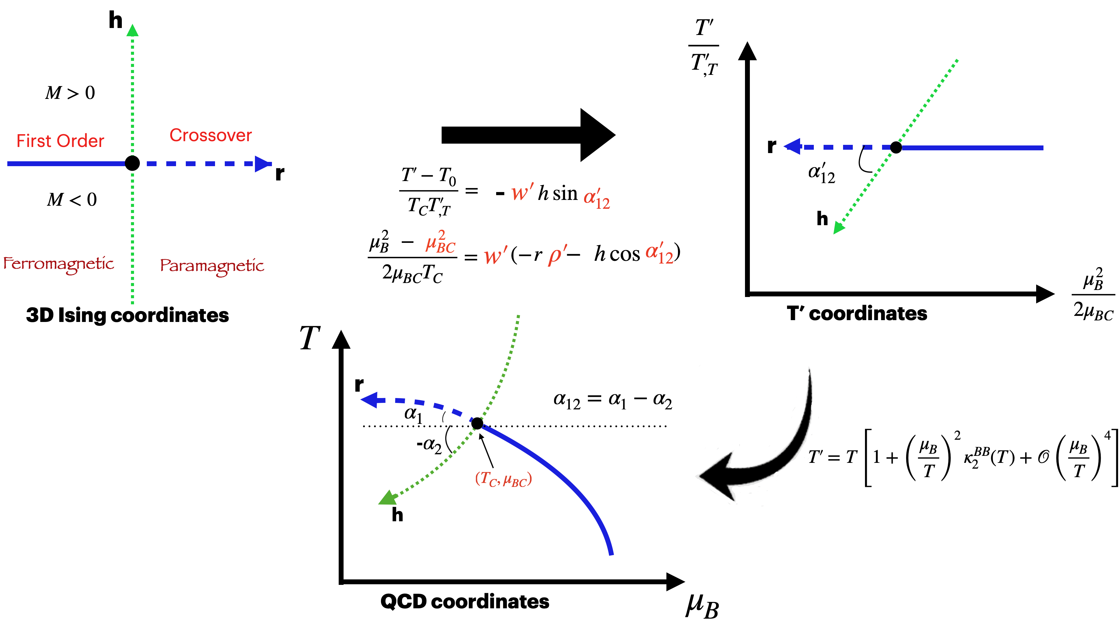
Figure 3: The top-left plot represents the 3D Ising model axes, with a critical point located at $(r=0,h=0)$. The top-right plot displays the $T^{\prime}$-expansion scheme coordinates, with a critical point at $(T^{\prime}=T_{0},\mu_{B}=\mu_{BC})$. Finally, the bottom plot corresponds to the QCD coordinates, featuring a critical point located at $(T_{C},\mu_{BC})$. The parameters in red $\mu_{BC}$, $w^{\prime}$,$\ \rho^{\prime}$ and $\alpha^{\prime}_{12}$ are the free parameters.

The mapping in Fig. 3 comes with inherent advantages. The tunable free parameters can be guided by physics, such as the physical value of the quark masses, stability, and causality of the equation of state [73]. This feature enables us to transport any physical quantity in 3D Ising to any point in the QCD phase diagram, and as the mapping is an even function in the baryon chemical potential, it ensures the expected charge conjugation symmetry.

III.3 Transition Line

With the mapping defined in Eq.(13), the location of the transition line in the phase diagram is naturally determined. The transition line $T_{C}(\mu_{BC})$ is such that $T_{C}$ and $\mu_{BC}$ have to satisfy $T^{\prime}(T,\mu_{B})=T_{0}$, where $T_{0}$ is the crossover temperature at $\mu_{B}=0$. For convenience, we use the pseudo-critical temperature related to chiral symmetry restoration $T_{0}=158$ MeV computed from the lattice in [9]. In addition, for simplicity, we identify $T^{\prime}$ with $T^{\prime}_{\text{lat}}(T,\mu_{B})$ in [13] up to second order in $\mu_{B}/T$. From Eq. (12), we make use of the mapping to express the critical pressure $P^{\rm crit}$ as a function of temperature and chemical potential:

$$P^{\rm crit}(T,\mu_{B})=-T^{4}G(R(T,\mu_{B}),\theta(T,\mu_{B}))\,\,.$$ (19)

The critical baryon density is then defined as

$$\chi_{1}^{\rm crit}=\frac{n_{B}^{\rm crit}(T,\mu_{B})}{T^{3}}=\frac{\partial(P^{\rm crit}(T,\mu_{B})/T^{4})}{\partial(\mu_{B}/T)}\Big{|}_{T}\,\,.$$ (20)

With this mapping the critical point is also forced to sit on the transition line by construction. Therefore, the number of free parameters is reduced since the critical temperature follows from the choice of critical chemical potential, and the angle $\alpha_{1}$ is given by the slope of the transition line at the critical point:

$$\alpha_{1}=\tan^{-1}\left(\frac{2\kappa_{2}(T_{C})\mu_{BC}}{T_{C}T^{\prime}_{,T}}\right)\;.$$ (21)

In this paper, we illustrate two choices of critical baryon chemical potential. The first one, used mainly for comparison with the BEST collaboration EoS, is $\mu_{BC}=350~{}\text{MeV}$, giving $T_{C}=140~{}\text{MeV}$ and $\alpha_{1}=6.7^{\circ}$. For the first choice of parameters, we show in Fig. 4 contours of equal normalized critical pressure, in the $r-h$, $T^{\prime}-\mu_{B}^{2}$ and $T-\mu_{B}$ planes. The first order transition line is shown as a red solid line, and the critical point corresponds to a black dot. We show positive and negative values of $\mu_{B}$, corresponding to positive and negative baryon chemical potentials, to illustrate the symmetry of QCD under baryon-and-antibaryon exchange. This symmetry arises naturally from the selection of a quadratic mapping of the chemical potential in Eq. (13). For the same choice of parameters, in Fig. 5 we show the critical baryon density, which develops a discontinuity for $\mu_{B}>\mu_{BC}$, as required for a first order transition. With the second choice we place the critical point in a region which goes beyond the limits of the BEST collaboration EoS: we choose $\mu_{BC}=500~{}\text{MeV}$, corresponding to $T_{C}=116~{}\text{MeV}$ and $\alpha_{1}=11.2^{\circ}$.

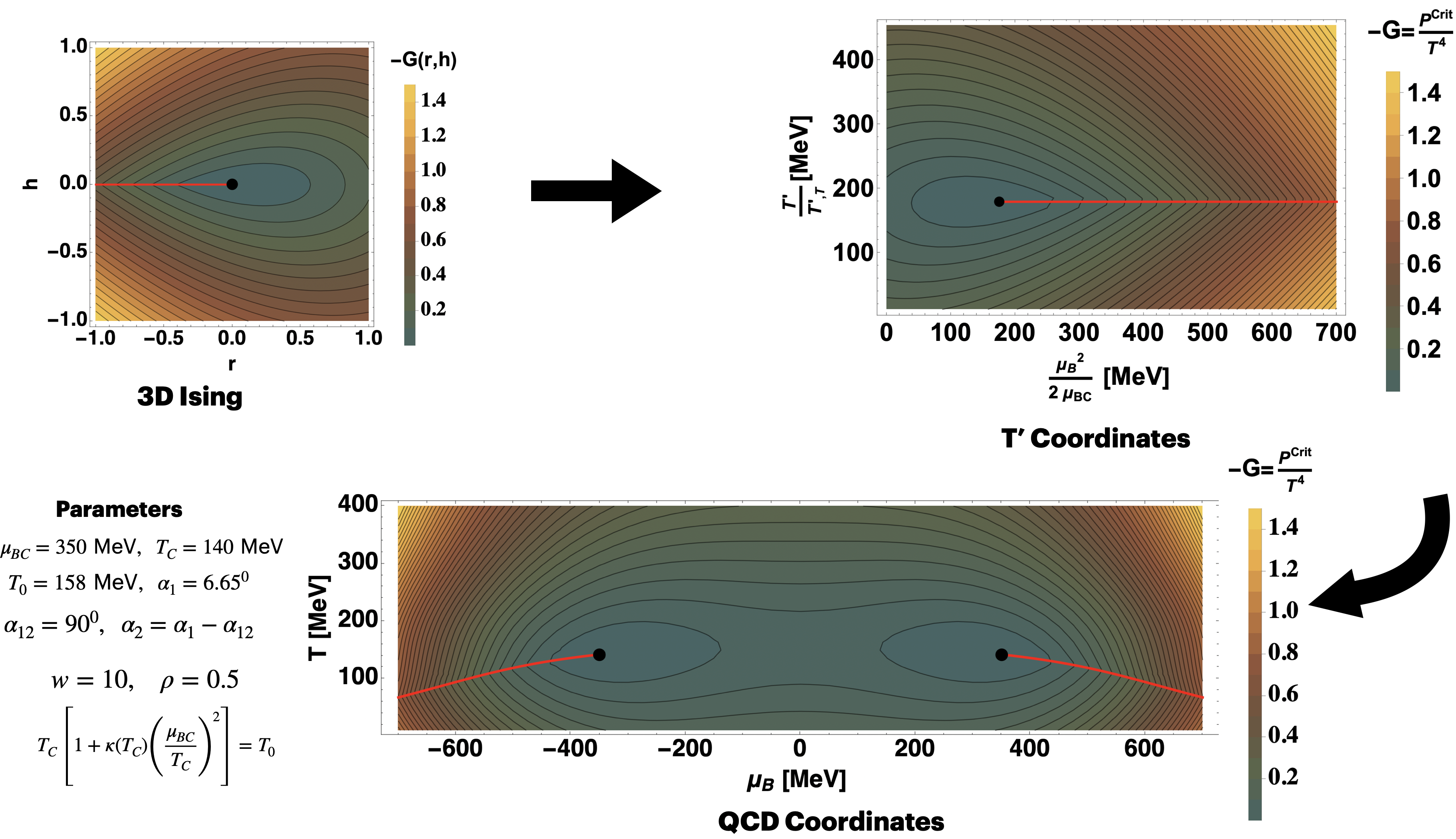
Figure 4: The figure comprises three contour plots of the critical (singular) contribution to pressure, in three different coordinate systems related to each other by transformations shown in Fig.3. The top-left plot uses the Ising model coordinates $(h,~{}r)$, with the critical point located at $(0,0)$. The top-right plot uses coordinates $(T/T^{\prime}_{,T},\mu_{B}^{2}/(2\mu_{BC}))$, with the critical point at $(T_{0}/T^{\prime}_{,T},\mu_{BC}/2)$. The bottom plot shows the same pressure in QCD coordinates $(\mu,T)$, featuring critical points located at $(\mu_{BC}=\pm 350~{}\text{MeV},~{}~{}T_{C}=140.1~{}\text{MeV})$. In all panels, the black dot represents the critical point and the red solid line denotes the first-order transition line.

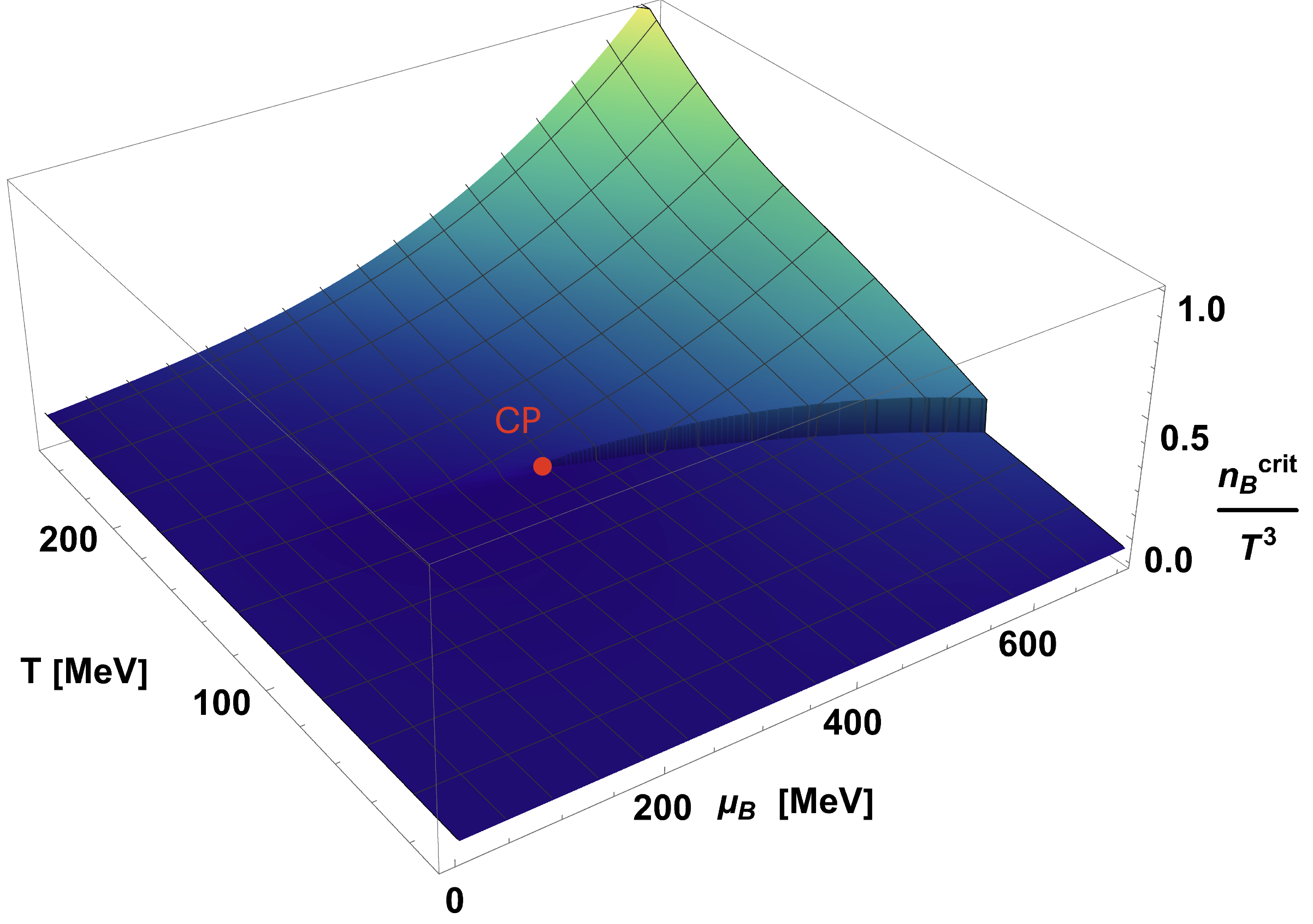
Figure 5: Critical baryon density for the chosen parameters $w=2,\rho=2$, $\alpha_{12}=90^{0}$ with the critical point at $\mu_{BC}=350$ MeV and $T_{C}=140~{}\text{MeV}$. For $\mu_{B}<\mu_{BC}$, no significant changes occur, indicating a smooth crossover transition. However, for $\mu_{B}>\mu_{BC}$, a distinct jump appears, marking the transition as first-order.

IV Equation of State: Merging the lattice data and the critical point singularity

It is important to keep in mind that equation (4) is the definition of $T^{\prime}(T,\mu_{B})$. Since the function $\chi_{2}^{B}(T^{\prime},0)$ is analytic (smooth crossover), the singularity in $n_{B}$ due to the critical point and the first-order transition must be carried by $T^{\prime}(T,\mu_{B})$. Since the singularity of $n_{B}$ is inherited from the singularity of the pressure via Eq. (20), we can determine the corresponding singularity in $T^{\prime}$ via equation (4).

We shall separate the baryon density into a regular and singular parts: $n_{B}=n_{B}^{\rm reg}+n_{B}^{\rm crit}$, where $n_{B}^{\rm crit}$ is defined by Eq.(20). Similarly, we separate $T^{\prime}$: $T^{\prime}=T^{\prime}_{\rm reg}+T^{\prime}_{\rm crit}$. Since $n_{B}^{\rm crit}$ vanishes at the critical point we can expand $\chi_{2}^{B}$ in Eq.(4) and obtain the relationship between $T^{\prime}_{\rm crit}$ and $n_{B}^{\rm crit}$:

$$T^{\prime}_{\rm crit}(T,\mu_{B})=\left(\frac{\partial\chi^{B}_{2}(T,0)}{\partial T}\Big{|}_{T_{0}}\right)^{-1}\frac{n^{\rm crit}_{B}(T,\mu_{B})}{T^{3}\times(\mu_{B}/T)}$$ (22)

Of course, the Taylor expansion of $T^{\prime}_{\rm crit}$ is different from Eq.(5) inferred from lattice data. However, we can always choose the regular $T^{\prime}_{\rm reg}$ contribution so that the Taylor expansion of the full $T^{\prime}$ agrees with the lattice. To match lattice results at low $(\mu_{B}/T)$, since $\kappa_{4}^{BB}(T)$ is consistent with zero, we can truncate the Taylor expansion in Eq.(5) and define

$$T^{\prime}_{\rm lat}(T,\mu_{B})=T\left(1+\kappa_{2}^{BB}(T)\left(\frac{\mu_{B}}{T}\right)^{2}\right).$$ (23)

We can then write

$$T^{\prime}(T,\mu_{B}) =\underbrace{T^{\prime}_{\rm lat}(T,\mu_{B})}_{\text{lowest orders in $(\mu_{B}/T)$ }}+$$

$$\qquad\underbrace{T^{\prime}_{\rm crit}(T,\mu_{B})-\text{Taylor}_{n\leq 2}[T^{\prime}_{\text{\rm crit}}(T,\mu_{B})]}_{\text{higher orders in $(\mu_{B}/T)$ }}\,\,,$$ (24)

which has the same singularity as $T^{\prime}_{\rm crit}$ and the same truncated Taylor expansion as $T^{\prime}_{\rm lat}$.

The last term in Eq.(24) represents the Taylor-expansion of $T^{\prime}_{\rm crit}(T,\mu_{B})$, which we will carry out to order $\mathcal{O}((\mu_{B}/T)^{2})$ and truncate beyond that order. Using Eq.(22) we find:

$$\text{Taylor}_{n\leq 2}[T^{\prime}_{\text{\rm crit}}] =\left(\frac{\partial\chi_{2,\rm lat}^{B}(T)}{\partial T}\bigg{|}_{T_{0}}\right)^{-1}\bigg{[}\frac{\partial n_{B}^{\text{\rm crit}}/T^{3}}{\partial(\mu_{B}/T)}\bigg{|}_{\hat{\mu}_{B}=0}$$

$$\quad+\frac{1}{3!}\frac{\partial^{3}n_{B}^{\text{\rm crit}}/T^{3}}{\partial(\mu_{B}/T)^{3}}\bigg{|}_{\hat{\mu}_{B}=0}\left(\frac{\mu_{B}}{T}\right)^{2}\bigg{]}.$$ (25)

One can thus identify the regular contribution $T^{\prime}_{\rm reg}$, using Eq.(24), as $T^{\prime}_{\rm reg}=T^{\prime}_{\rm lat}-\text{Taylor}_{n\leq 2}[T^{\prime}_{\text{\rm crit}}]$.

At this point, inserting Eq. (24) in (4) completely defines the baryon density with a critical point for a chosen set of critical point parameters. As an example, we show in Fig. 6 the baryon density as a function of the temperature, for different values of $\mu_{B}/T$, for a critical point located at $\mu_{BC}=350$ MeV, resulting in $T_{C}=140$ MeV, $\alpha_{1}=6.65^{\circ}$, with $\alpha_{2}=\alpha_{1}-\alpha_{12}$, $\alpha_{12}=90^{\circ}$, $w=2$ and $\rho=2$. We compare these results with lattice QCD results obtained in Ref. [13] from the alternative expansion scheme. Notably, we can see that our results are not in tension, within error bars, with the lattice ones, even when a critical point is placed in the chemical potential regime accessible to the extrapolation.

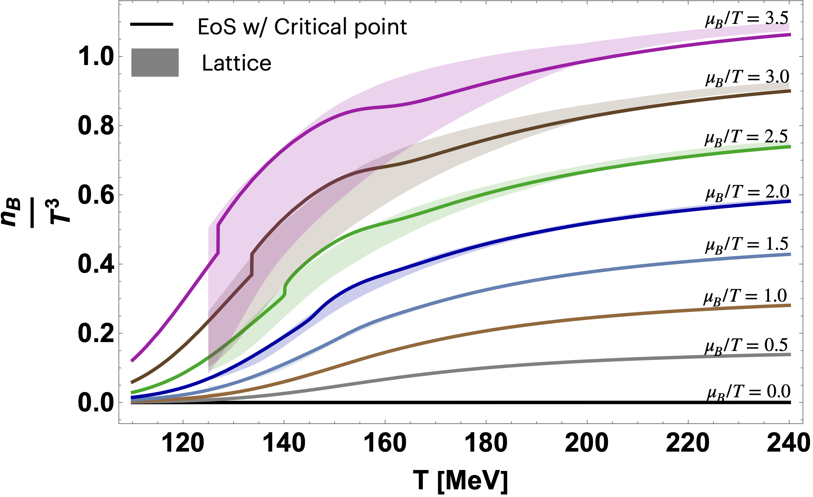
Figure 6: Baryon density as a function of the temperature, for different values of $\mu_{B}/T$. Solid lines correspond to the equation of state with a critical point located at $\mu_{BC}=350$ MeV resulting in $T_{C}=140~{}\text{MeV},~{}\alpha_{1}=6.65^{0}$, with $\alpha_{2}=\alpha_{1}-\alpha_{12},~{}\alpha_{12}=90^{0},~{}w=2$ and $\rho=2$. They are compared to lattice QCD results from Ref. [13] obtained using the $T^{\prime}$-expansion scheme, shown as bands indicating the errors due to Taylor expansion truncation.

V Results : Thermodynamics

In this section, we calculate all thermodynamic observables. From Eq. (4), the baryon density $n_{B}(T,\mu_{B})$ in temperature and chemical potential is readily provided, and the pressure $P(T,\mu_{B})$ is obtained through simple integration:

$$\frac{P(T,\mu_{B})}{T^{4}}=\chi_{0,\rm lat}^{B}(T,0)+\frac{1}{T}\int_{0}^{\mu_{B}}d\mu_{B}^{\prime}\frac{n_{B}(T,\mu_{B}^{\prime})}{T^{3}}\,\,.$$ (26)

The integration constant $\chi_{0,\rm lat}^{B}(T,0)$ is the pressure at $\mu_{B}=0$, for which we employ lattice QCD results from Ref. [10].

Entropy density, energy density and second baryon susceptibility are derivatives of pressure and baryon density, defined as:

$$\frac{s(T,\mu_{B})}{T^{3}} =\frac{1}{T^{3}}\frac{\partial P(T,\mu_{B})}{\partial T}\Big{|}_{\mu_{B}}$$ (27)

$$\frac{\epsilon(T,\mu_{B})}{T^{4}} =-\frac{P(T,\hat{\mu}_{B})}{T^{4}}+\frac{s(T,\hat{\mu}_{B})}{T^{3}}+\hat{\mu}_{B}\frac{n_{B}(T,\hat{\mu}_{B})}{T^{3}}$$ (28)

$$\chi_{2}^{B}(T,\mu_{B}) =\frac{\partial({n_{B}(T,\mu_{B})}/T^{3})}{\partial\mu_{B}/T}\bigg{|}_{T}$$ (29)

which we implement through Eqs. (34) and (35). In Figs. 7, 8, 9, and 10 we show the baryon density, pressure, second baryon susceptibility and energy density, respectively, as functions of the temperature, for different values of the baryon chemical potential. These correspond to a critical point located at $\mu_{BC}=500~{}\text{MeV}$, resulting in $T_{C}=117~{}\text{MeV}$ and $\alpha_{1}=11^{\circ}$. Additionally, we have $w=15$, $\rho=0.3$, and $\alpha_{12}=\alpha_{1}$, meaning $\alpha_{2}=\alpha_{1}-\alpha_{12}=0$.

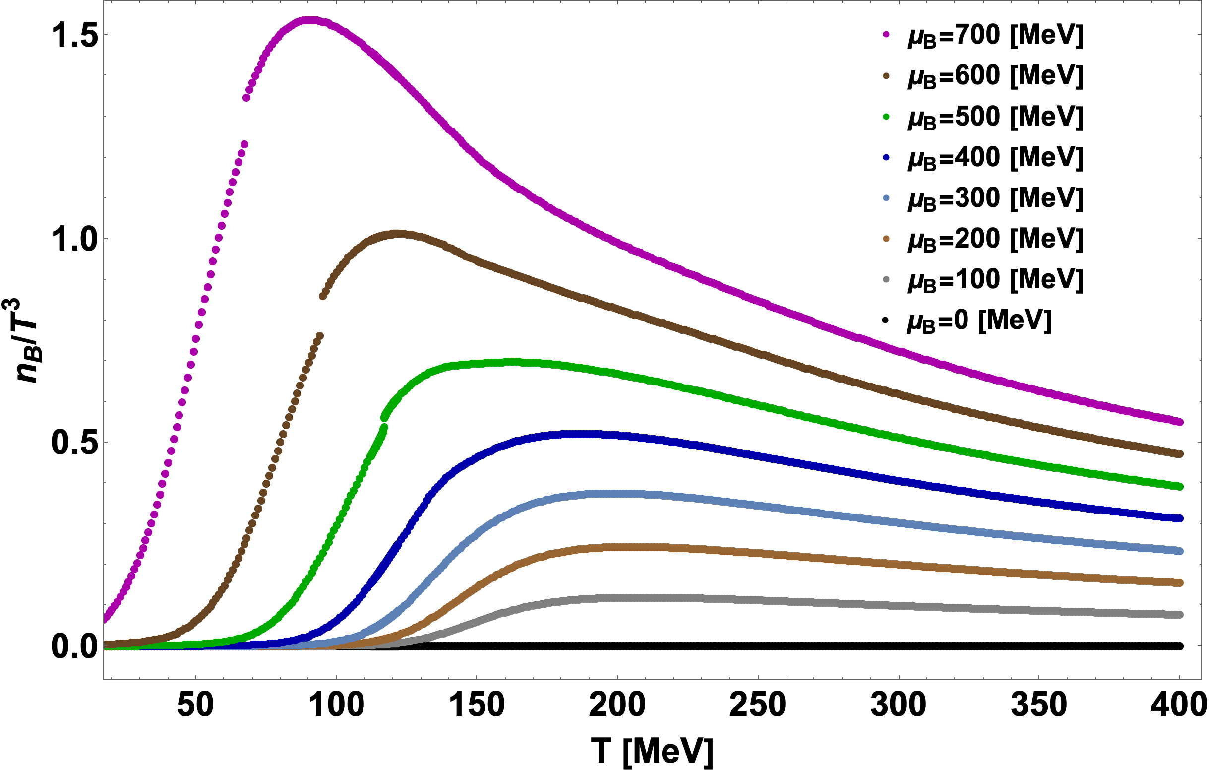
Figure 7: Baryon density as a function of the temperature for different baryon chemical potentials. As expected, a discontinuity appears when $\mu_{B}>\mu_{BC}$, where the transition is first order. The critical point is located at $\mu_{BC}=500~{}\text{MeV}$, resulting in $T_{C}=117~{}\text{MeV}$ and $\alpha_{1}=11^{\circ}$. Additionally, we have $w=15$, $\rho=0.3$, and $\alpha_{12}=\alpha_{1}$, meaning $\alpha_{2}=\alpha_{1}-\alpha_{12}=0$.

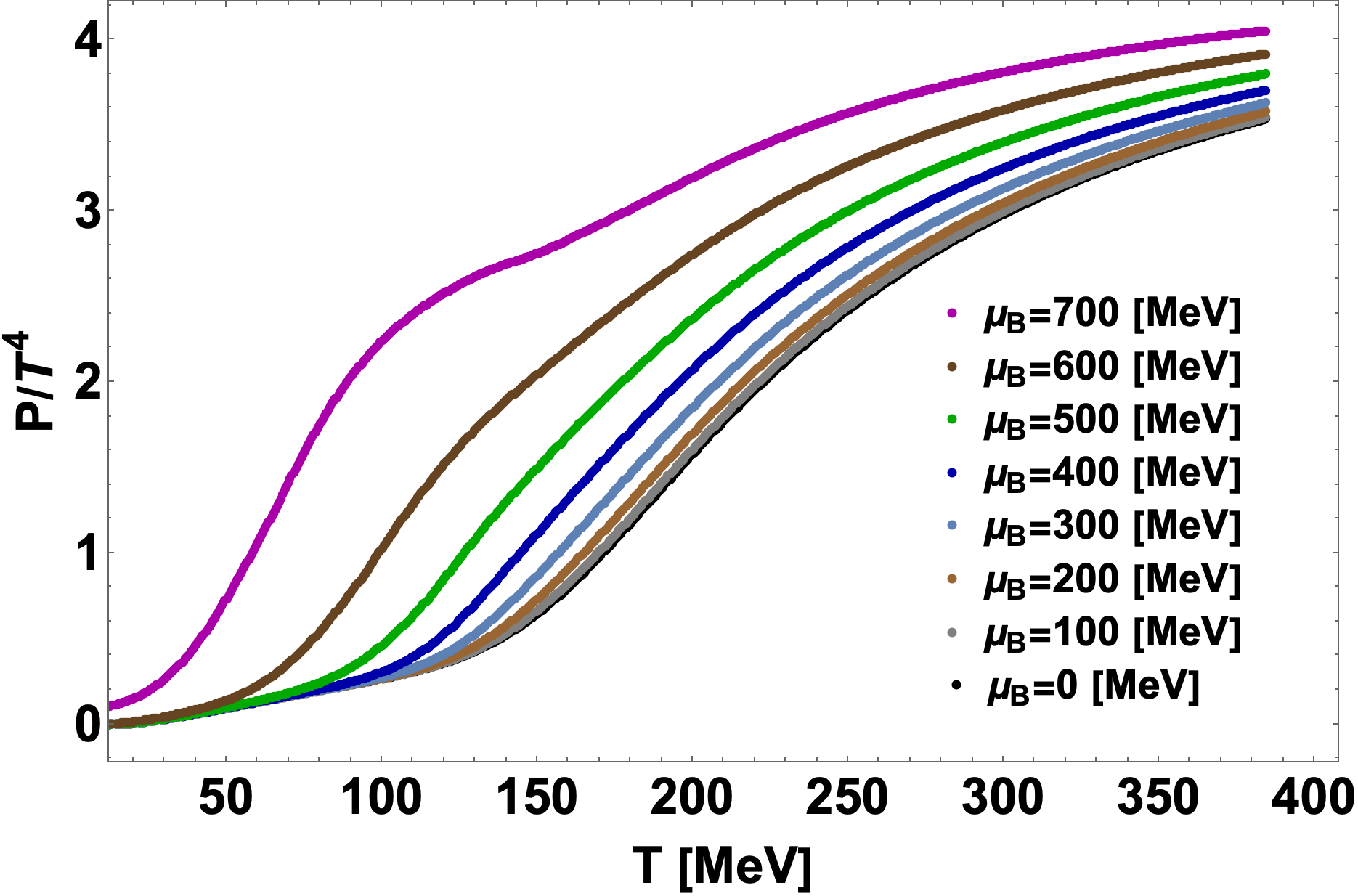
Figure 8: Pressure as a function of the temperature for different baryon chemical potentials. The critical point manifests itself less clearly in the pressure, which only develops a kink for $\mu_{B}>\mu_{BC}$. The plot corresponds to the same parameters as the ones used in Fig. 7.

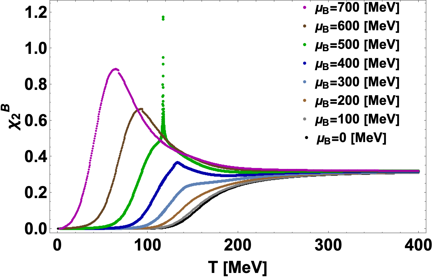
Figure 9: Second order baryon susceptibility as a function of the temperature for different baryon chemical potentials. This quantity represents the measure of how baryon density reacts to an increase in chemical potential. A divergence is expected at the critical point, which can be seen for $\mu_{B}=\mu_{BC}=500\,\text{MeV}$. The plot corresponds to the same parameters as the ones used in Fig. 7.

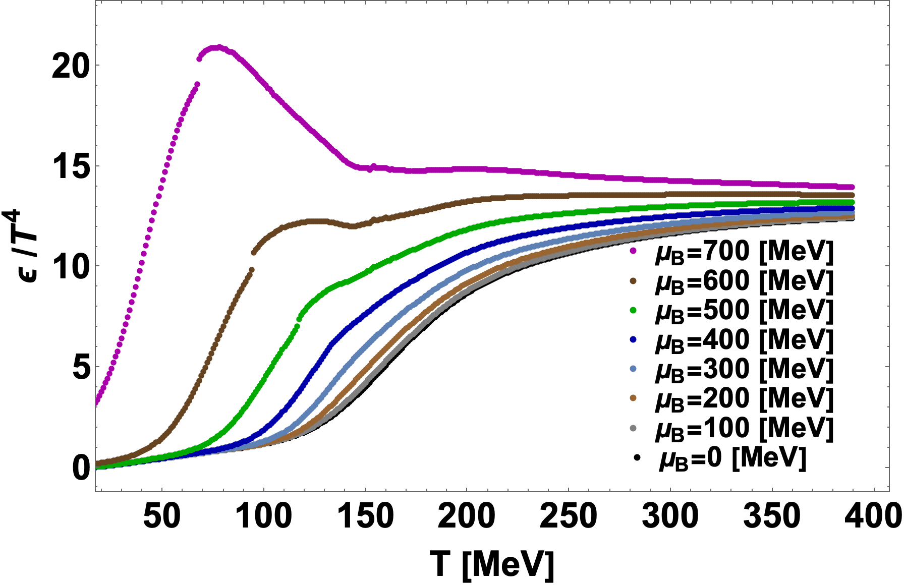
Figure 10: Energy density as a function of the temperature for different baryon chemical potentials. This quantity also shows a discontinuity for $\mu_{B}>\mu_{BC}$. The plot corresponds to the same parameters as the ones used in Fig. 7.

VI Constraints on the EoS

In this manuscript, we obtain a family of equations of state which depend on the free parameters $\mu_{BC}$, $w$, $\rho$ and $\alpha_{12}$ introduced by the mapping in Eq. (3). However, the values of these parameters can be guided by physics and the current knowledge from experiments, in order to constrain them and obtain a physical equation of state that describes strongly interacting matter.

VI.1 Lattice Results

While our equations of state depend on the free parameters at high $\mu_{B}$, we require that they all reproduce lattice QCD results for pressure and its $\mu_{B}$ derivatives up to 4th order at $\mu_{B}=0$. This can be inferred from Fig. 6, where we compare our baryon density (exhibiting a discontinuity at $\mu_{B}>\mu_{BC}$) with the lattice QCD results from Ref. [13]: within error-bars, our discontinuity does not contradict the results from lattice QCD.

VI.2 Physical Quark masses

In Ref. [73], a thorough investigation was conducted regarding the linear mapping from Ising to QCD introduced in Refs. [51, 81]. This study effectively explored the scenario in which the critical point closely approaches the tricritical point, revealing a universal dependence of the mapping parameters on the quark mass $m_{q}$. Notably, when the critical point resides in the proximity of the tricritical point, the angle denoted as $\alpha_{12}$ between the lines of $r=0$ and $h=0$ within the $(T,\mu_{B})$ plane decreases, exhibiting a behavior proportional to $m_{q}^{2/5}$. For a physical quark mass $m_{q}$, the angle $\alpha_{12}\approx\alpha^{\prime}_{12}$ as in (43a) needs to be small, approximately equal to $\alpha_{1}$.

VI.3 Stability and Causality

The non-universal mapping from $(r,h)$ to $(T,\mu_{B})$ leaves open the selection of free parameters. While the angle $\alpha_{12}$ can be constrained by the physical value of the quark masses, there is no physical guidance for the scaling parameters $(w,\rho)$. Potentially, some choices of parameters would lead to an unstable equation of state.

For a valid equation of state, certain conditions must be met. We require that the pressure is a monotonically increasing function of $T$ and $\mu_{B}$, which means positivity of baryon density, entropy density, energy density, speed of sound, and baryon number susceptibility everywhere in the $(T,\mu_{B})$ plane [82] ranging from $0<\mu_{B}<700$ MeV and $25\,\text{MeV}<T<800$ MeV. This can be summarized in two conditions: positivity of the second baryon susceptibility $\chi_{2}$ and of the specific heat at constant volume $c_{V}$, which can be written as [83]:

$$c_{V}(T,\mu_{B})= \frac{T}{\chi_{2}^{B}}\left[\frac{\partial s}{\partial T}\chi_{2}^{B}-\left(\frac{\partial n_{B}}{\partial T}\right)^{2}\right]\,\,.$$ (30)

Additionally, to uphold causality, the speed of sound

$$c_{s}^{2}(T,\mu_{B})=\left(\frac{\partial p}{\partial\epsilon}\right)_{s/n}=\frac{n^{2}\frac{\partial^{2}p}{\partial T^{2}}-2sn\frac{\partial^{2}p}{\partial T\partial\mu_{B}}+s^{2}\frac{\partial^{2}p}{\partial\mu_{B}^{2}}}{(\epsilon+p)\left(\frac{\partial^{2}p}{\partial T^{2}}\frac{\partial^{2}p}{\partial\mu_{B}^{2}}-\left(\frac{\partial^{2}p}{\partial T\partial\mu_{B}}\right)^{2}\right)}\,\,$$

must fall within the range $0\leq c_{s}^{2}\leq 1$. The behavior of the speed of sound as a function of $T$ and $\mu_{B}$ can be seen in Fig. 11. It exhibits a dip at the critical point, where it vanishes. We show in Fig. 12 a landscape of acceptable (blue triangles) and pathological (red squares) choices for the parameters $w$ and $\rho$, for a critical point located at $\mu_{BC}=500~{}\text{MeV}$, which corresponds to $T_{C}=117~{}\text{MeV}$ and $\alpha_{1}=11^{\circ}$. Additionally, we have $\alpha_{12}=\alpha_{1}$, meaning $\alpha_{2}=\alpha_{1}-\alpha_{12}$, while $w$ and $\rho$ are varied in the range $w=2.5-22.5$, $\rho=0.1-1.3$. Similar plots, comparing our parameter landscapes to the ones from the BEST collaboration EoS, are discussed in Appendix C.

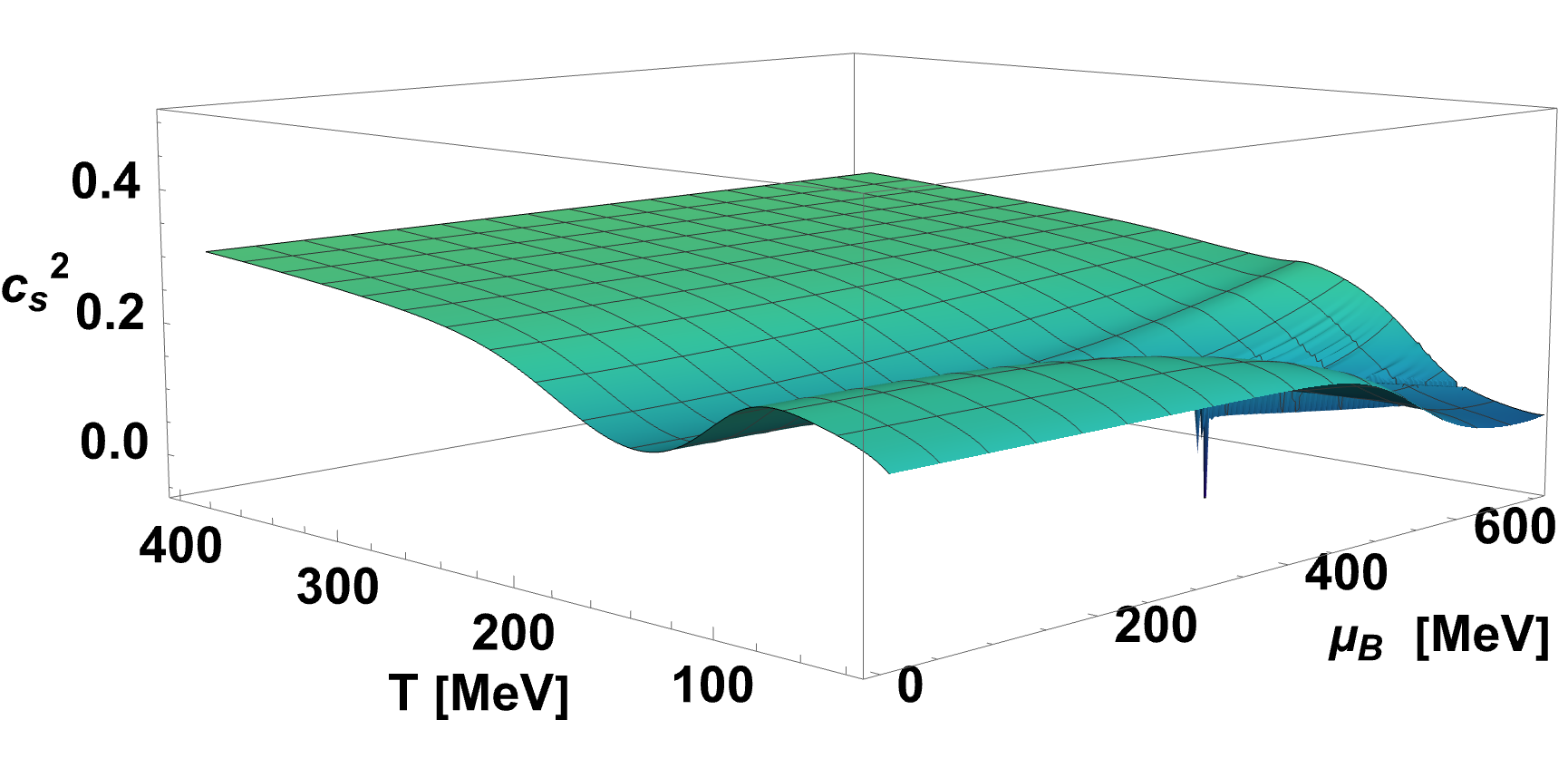
Figure 11: Speed of sound as a function of temperature and baryon chemical potential. This quantity shows a pronounced at the critical point. The plot corresponds to the same parameters as the ones used in Fig: 7.

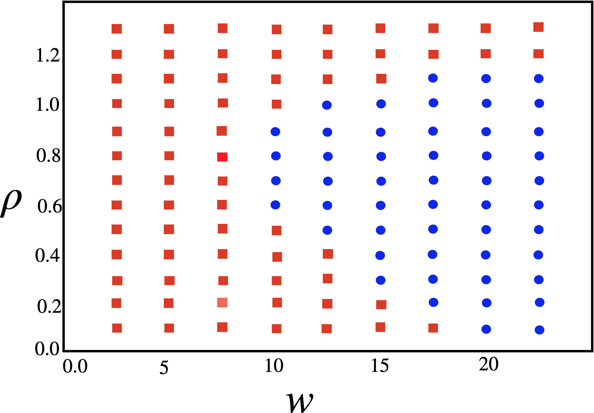
Figure 12: Landscape plot in the range $w=2.5-22.5$, $\rho=0.1-1.3$ at fixed values of $\mu_{BC}=500~{}\text{MeV},~{}T_{C}=117~{}\text{MeV},~{}\alpha_{1}=11^{0}$ and $\alpha_{12}=\alpha_{1}$. Red squares correspond to a pathological choice of parameters in the range $\mu_{B}=\{0,700~{}\text{MeV}\}$, while the blue dots represent acceptable ones.

VII Summary and Conclusions

Determining the QCD equation of state, in particular, establishing the existence of the QCD critical point and pinning down its location, is a major goal of heavy-ion collision experiments. The strategy based on comparing predictions of hydrodynamics sensitive to EoS with experiment requires a parametric family of EoS which can be fed into a hydrodynamic code. In this paper, we introduced a novel framework for constructing such a family of QCD equations of state.

Our framework improves on the BEST collaboration approach [51] by introducing several significant innovations. This allows us to achieve coverage over a wider range of the QCD phase diagram relevant for critical point searches.

The main innovation in our paper is merging the universal critical point singularity with the implementation of the $T^{\prime}$-expansion scheme [13]. The $T^{\prime}$-expansion scheme takes into account the observation that the temperature driven crossover looks remarkably similar at different chemical potentials, the main difference being a shift of the crossover temperature with increasing $\mu_{B}$. The “rescaled temperature” $T^{\prime}(T,\mu_{B})$ defined in Eq.(4) carries information about the dependence of the position and the shape of the crossover at different $\mu_{B}$. Since this dependence is relatively slow, the expansion of $T^{\prime}$, as in Eq.(5), is much better controlled than the expansion of quantities such as $\chi_{2}^{B}$, which vary rapidly at the crossover.

We introduce the critical singularity into the function $T^{\prime}(T,\mu_{B})$, while making sure that the Taylor expansion coefficients (at $\mu_{B}=0$) still agree with the lattice data.

Another innovation, relative to the BEST EoS framework, is the mapping of the Ising coordinates $r$ and $h$ into QCD coordinates $T$ and $\mu_{B}^{2}$, instead of $\mu_{B}$. This takes care of the charge conjugation symmetry and the associated curvature of the QCD pseudocritical line.

We check the novel framework by calculating quantities which must obey thermodynamic inequalities. Of course, for sufficiently large $\mu_{B}$ or for sufficiently strong critical point singularity, the framework will show its limitations by violating these inequalities. However, the range of parameters where the novel framework is thermodynamically consistent is larger than the same range for the BEST collaboration EoS family.

In particular, our framework allows us to provide thermodynamically consistent EoS in the range $\mu_{B}=0-700$ MeV, extending beyond the BEST EoS range $\mu_{B}=0-450$ MeV. In addition, the range for critical point parameters $w$ and $\rho$ is also extended compared to the one for the BEST EoS at similar values of $T$ and $\mu_{B}$.

There are several potential avenues for further improvement. Since the approach is still based on the Taylor expansion, necessarily truncated based on the availability of the lattice data, it inevitably breaks down at sufficiently large $\mu_{B}$. It might be possible to introduce additional resummation techniques dealing with these limitations at larger $\mu_{B}$. In addition, the true EoS of QCD possesses the well known periodicity in the complex plane: $\mu_{B}\to\mu_{B}+2\pi Ti$ due to the quantization of the baryon number. This periodicity could also be implemented. We leave these and further improvements to future work.

Appendix A Taylor expansion of the critical contribution

Here we present the formula and derivation for $\text{Taylor}[T^{\prime}_{\rm crit}(T,\mu_{B})]$. Since in our approach $T^{\prime}_{\rm lat}(T,\mu_{B})$ is truncated up to $\kappa_{2}(T)$, we need the $\text{Taylor}[T^{\prime}_{crit}(T,\mu_{B}),n=2]=a_{0}(T)+a_{2}(T)\left(\frac{\mu_{B}}{T}\right)^{2}$, such that we match that same order by construction, while the higher order contributions come from the critical part. The coefficients $a_{0}$ and $a_{2}$ are then given by;

$$a_{0}(T) =\left(\frac{\partial\chi_{2}}{\partial T}\bigg{|}_{T_{0}}\right)\left(\frac{\partial n_{B}^{\rm crit}(T,\mu_{B})}{\partial(\mu_{B}/T)}\right)\bigg{|}_{\mu_{B}/T=0}$$ (32)

$$a_{2}(T) =\left(\frac{\partial\chi_{2}}{\partial T}\bigg{|}_{T_{0}}\right)\left(\frac{1}{3!}\frac{\partial^{3}n_{B}^{\rm crit}(T,\mu_{B})}{\partial(\mu_{B}/T)^{3}}\right)\bigg{|}_{\mu_{B}/T=0}$$ (33)

Appendix B Computing thermodynamics

From Eq. (4), we obtain Eq. (34) and Eq. (35), which are derivatives of the baryon density with respect to chemical potential and temperature, respectively

$$\frac{\partial n_{B}(T,\mu_{B})}{\partial(\mu_{B}/T)}=\chi_{2,\rm lat}^{B}(T^{\prime})T^{3}+$$

$$\frac{\mu_{B}}{T}\frac{\partial\chi_{2,\rm lat}^{B}(T)}{\partial T}\bigg{|}_{T^{\prime}}\frac{\partial T^{\prime}}{\partial(\mu_{B}/T)}T^{3}$$ (34)

$$\frac{\partial n_{B}(T,\mu_{B})}{\partial T}=2\frac{n_{B}(T,\mu_{B})}{T}+$$

$$\frac{\mu_{B}}{T}\frac{\partial\chi_{2,\rm lat}(T)}{\partial T}\frac{\partial T^{\prime}}{\partial T}T^{3}$$ (35)

Then entropy is computed from the integral of Eq. (35) using

$$s(T,\mu_{B}) =4T^{3}\chi_{0,\rm lat}^{B}(T)+T^{4}\frac{\chi_{0,\rm lat}^{B}(T)}{dT}$$

$$\int_{0}^{{\mu}_{B}}d{\mu}_{B}^{\prime}\frac{\partial n_{B}(T,\mu_{B}^{\prime})}{\partial T}$$ (36)

All thermodynamic quantities, calculated in this paper as functions of temperature and chemical potential, are shown in Figures 7-10 and 13-16 for slices at constant $\mu_{B}$ in the main text and 3D plots in the Appendix, respectively.

Appendix C Comparison with BEST EoS

In [51, 73, 82], a linear map from Ising to QCD with six parameters was utilized.

$$T-T_{C} = T_{C}w(r\rho\sin\alpha_{1}+h\sin\alpha_{2})$$

$$\mu_{B}-\mu_{BC} = T_{C}w(-r\rho\cos\alpha_{1}-h\cos\alpha_{2}).$$ (37)

By making use of the following equations for the slopes at the critical point:

$$\frac{dT}{d\mu_{B}}\Big{|}_{h=0} =-\tan\alpha_{1}$$ (38)

$$\frac{dT}{d\mu_{B}}\Big{|}_{r=0} =-\tan\alpha_{2}$$ (39)

and linearizing Eq. (13) around the critical point and using $T^{\prime}_{\text{lat}}=T\left(1+\kappa_{2}(T)\left(\frac{\mu_{B}}{T}\right)^{2}\right)$,

$$\frac{1}{T^{\prime}_{,T}}\frac{\Delta T^{\prime}}{\Delta\mu_{B}}=\frac{\Delta T}{\Delta\mu_{B}}+\frac{2\kappa_{2}(T)\mu_{B}}{T^{\prime}_{,T}T}$$ (40)

At $h=0$, we get Eq.(21):

$$\tan\alpha_{1}=\frac{2\kappa_{2}(T_{C})\mu_{BC}}{T^{\prime}_{,T}T_{C}}$$ (41)

At $r=0$, we get Eq. (14a):

$$\tan\alpha^{\prime}_{12}=\tan\alpha_{1}-\tan\alpha_{2}$$ (42)

Using simple trigonometric relations and Eq.(16) and Eq.(17), we find (14b) and (14c).

Then, we approximate for either small angles or large angles:

• For small angles:

  $$\alpha_{12}^{\prime}\approx\alpha_{12}\,;$$ (43a)

  $$w^{\prime}\approx w\,;$$ (43b)

  $$\rho^{\prime}\approx\rho\,;$$ (43c)

• For $\alpha_{1}\ll 1$ and $\alpha_{12}=90^{\circ}$:

  $$\alpha_{12}^{\prime} \approx 90^{\circ}-\alpha_{1}\,;$$ (44a)

  $$w^{\prime} \approx w\,;$$ (44b)

  $$\rho^{\prime} \approx\rho\,.$$ (44c)

In Figures 17 and 18, we compare the stability parameter landscape in $w$ and $\rho$ for our approach to the ones from the BEST collaboration EoS. In Fig. 17, the Ising model axes are chosen to be orthogonal to each other. However, since physically motivated values of the angle $\alpha_{12}$, characterizing the shape of the critical region, are small [73], it is important that the improvement in the $w$ and $\rho$ ranges is especially pronounced for small angle $\alpha_{12}$, as shown in Fig.18 for $\alpha_{2}=0$, i.e., $\alpha_{12}=\alpha_{1}$. From these figures it is clear that the quadratic mapping in Fig: 3 has more acceptable points than the linear mapping in [51].

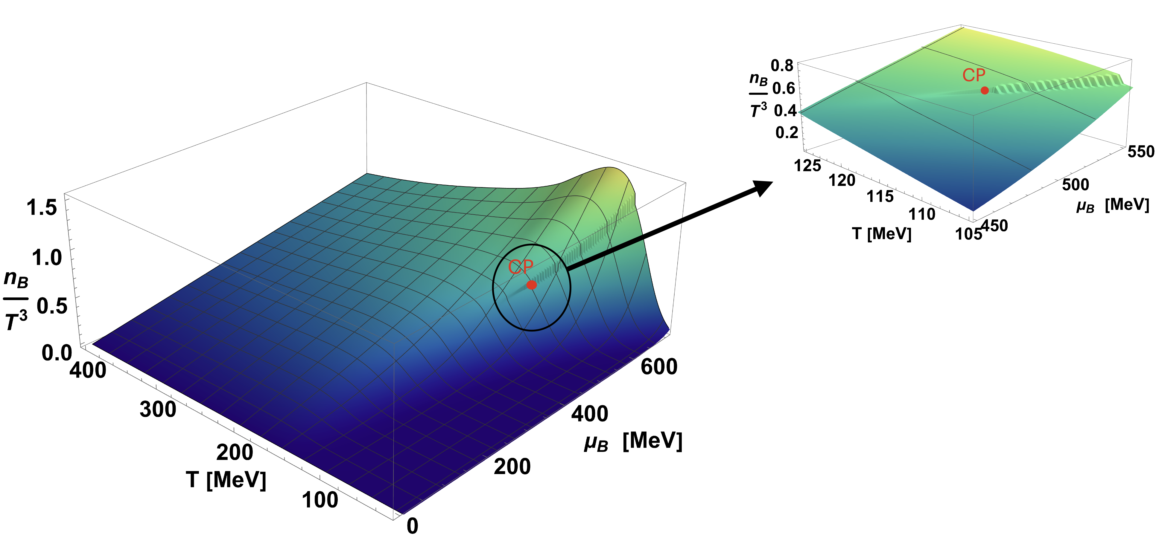
Figure 13: Baryon density as a function of temperature and chemical potential for the same parameters as in Fig. 7, with a zoom into the critical region.

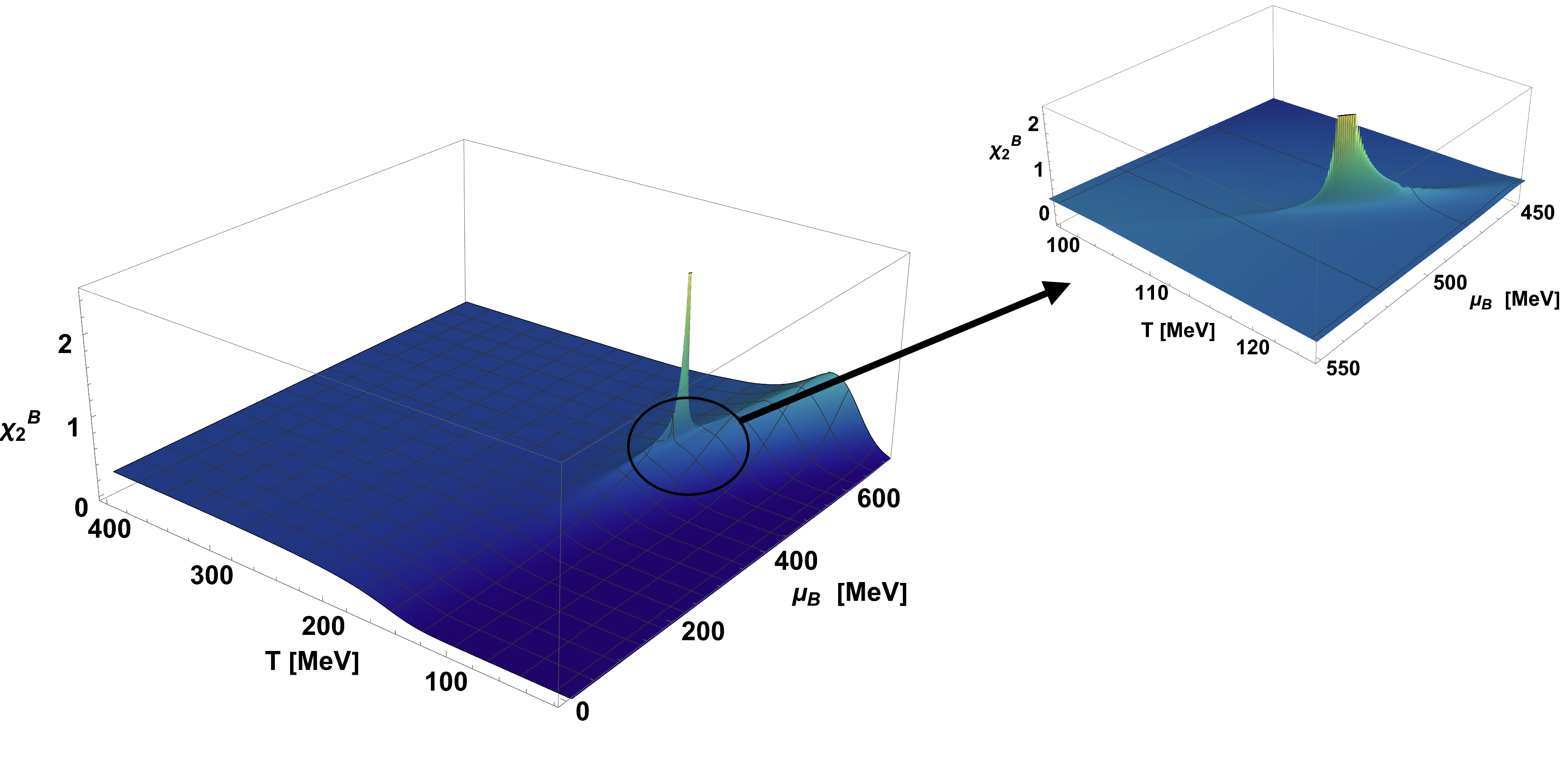
Figure 14: Second baryon number susceptibility as a function of temperature and chemical potential for the same parameters as in Fig. 7, with a zoom into the critical region

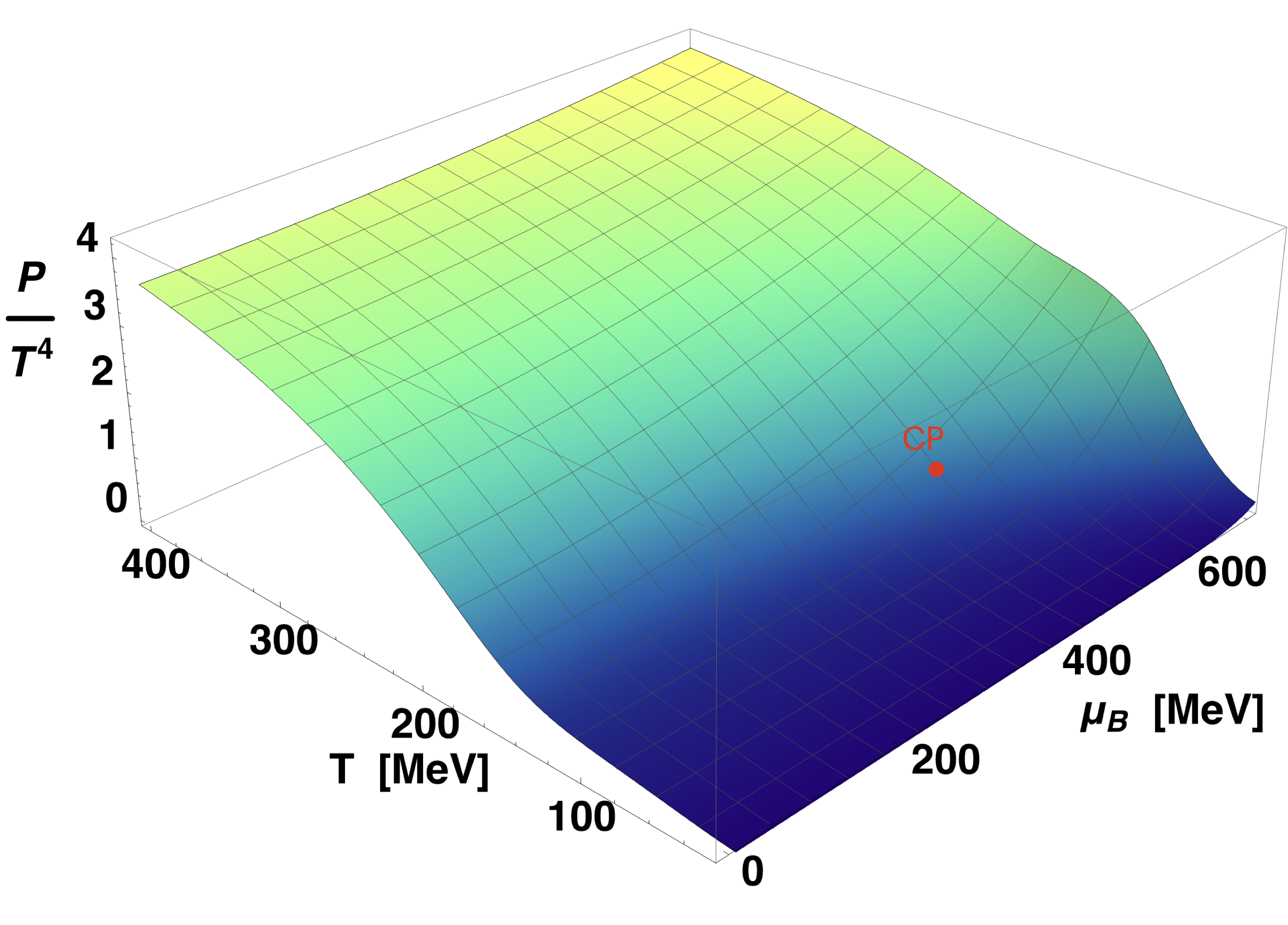
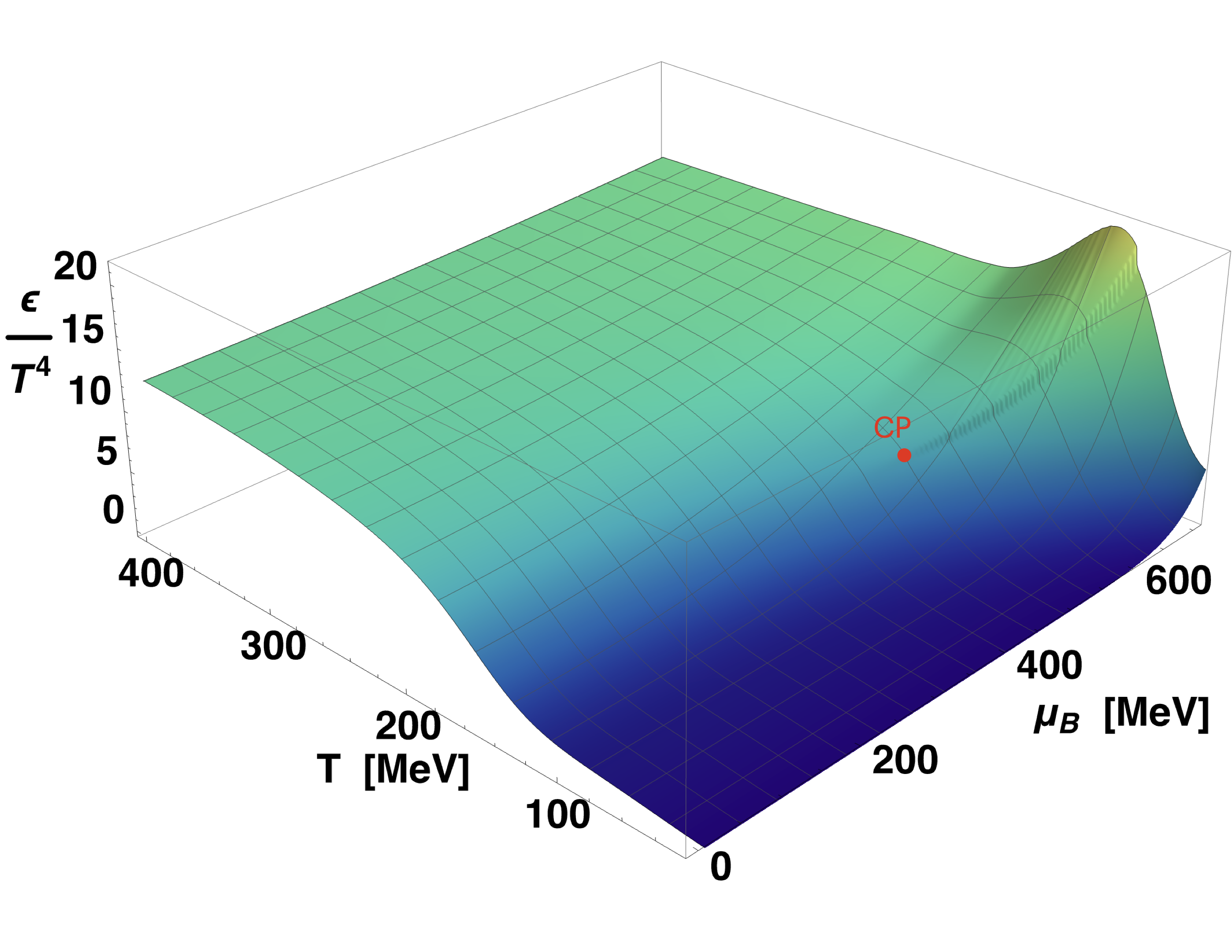
Figure 15: Pressure on the left panel and Energy density on the right panel with a red point representing a critical point for the same parameters as in Fig. 7

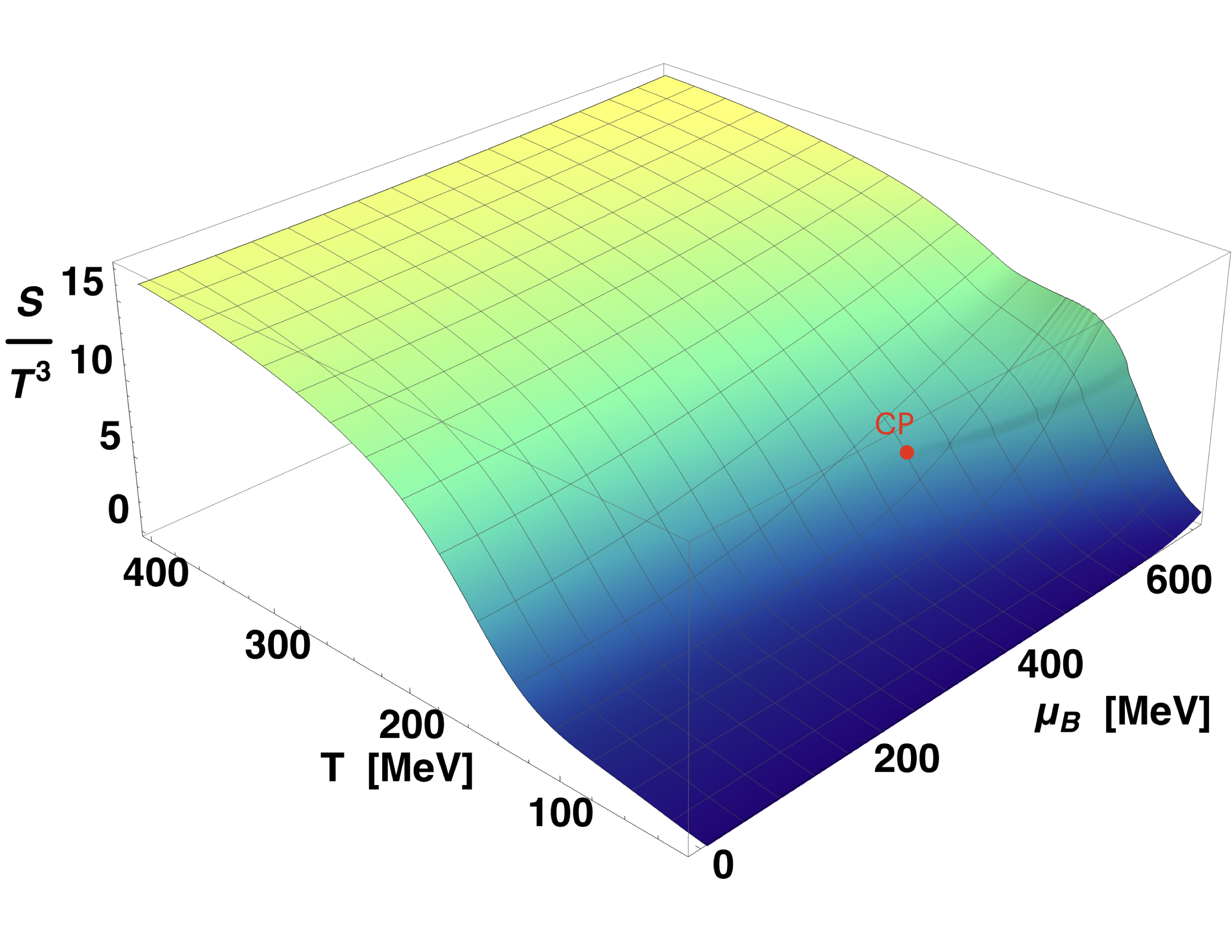
Figure 16: Entropy density as a function of temperature and chemical potential with a red point representing a critical point for the same parameters as in Fig. 7

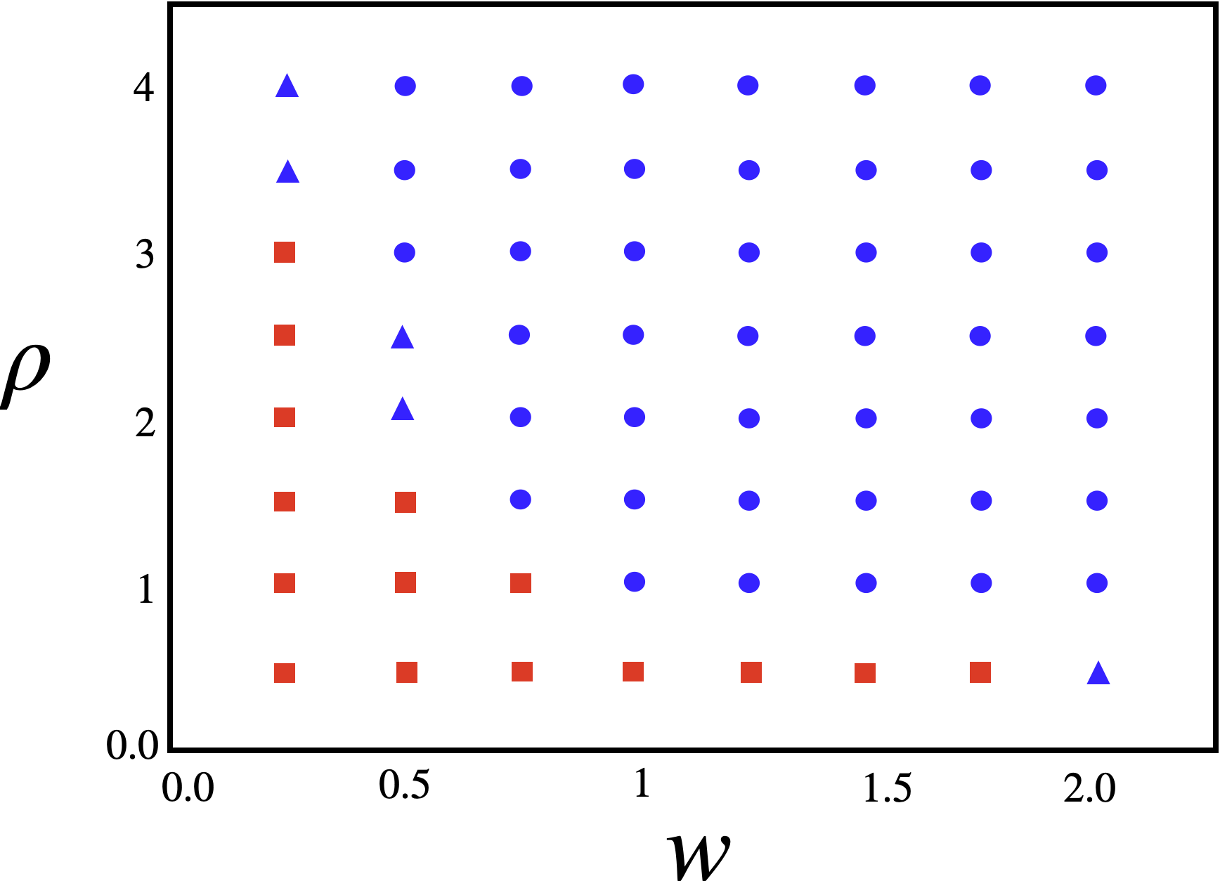
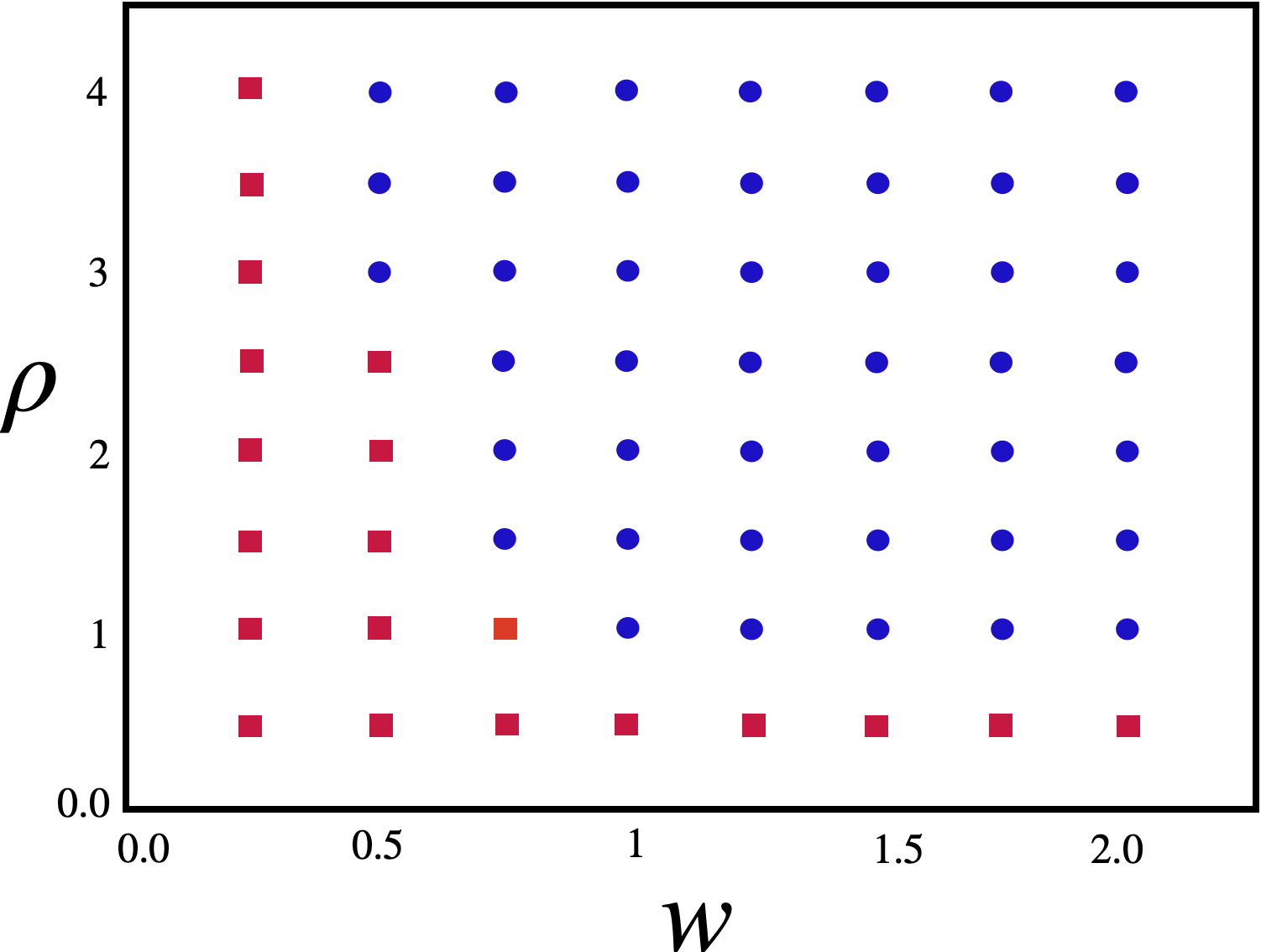
Figure 17: Comparison of the stability plots for $w$ and $\rho$ with the new mapping (Quadratic) on the left panel and the BEST mapping (Linear) [51] on the right. The blue points represent acceptable parameters, while the red points denote unacceptable ones for $\mu_{BC}=350\,\text{MeV},T_{C}=140.073\,\text{MeV},\alpha_{1}=6.653^{\circ},\kappa=0.02633$ with $\alpha_{12}=90^{\circ}$ for $\mu_{B}=\{0,450\text{MeV}\}$. Blue triangles on the left panel indicate parameters that are acceptable in the new mapping, while they were not in the BEST collaboration mapping.

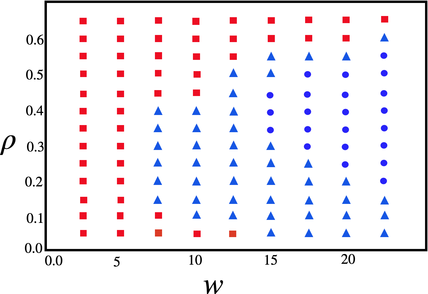
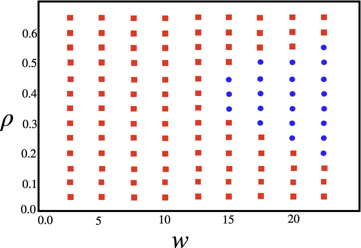
Figure 18: Comparison of the stability plots for $w$ and $\rho$ with the new mapping (Quadratic) on the left panel and the BEST collaboration mapping (Linear) [51] on the right. The blue points represent acceptable parameters, while the red points denote unacceptable ones for $\mu_{BC}=350\,\text{MeV},T_{C}=140.073\,\text{MeV},\alpha_{1}=6.653^{\circ},\kappa=0.02633$ with $\alpha_{2}=0$, i.e., $\alpha_{12}^{\prime}=\alpha_{12}=\alpha_{1}$ for $\mu_{B}=\{0,450\text{MeV}\}$. Blue triangles on the left panel indicate parameters that are acceptable in the new mapping, while they were not in the BEST collaboration mapping.

References

- Stephanov [2004] M. A. Stephanov, QCD phase diagram and the critical point, Prog. Theor. Phys. Suppl. 153, 139 (2004), arXiv:hep-ph/0402115 .
- Ratti [2023] C. Ratti, Equation of state for QCD from lattice simulations, Prog. Part. Nucl. Phys. 129, 104007 (2023).
- [3] R. Kumar et al. (MUSES), Theoretical and Experimental Constraints for the Equation of State of Dense and Hot Matter, arXiv:2303.17021 [nucl-th] .
- Aoki et al. [2006] Y. Aoki, G. Endrodi, Z. Fodor, S. D. Katz, and K. K. Szabo, The Order of the quantum chromodynamics transition predicted by the standard model of particle physics, Nature 443, 675 (2006), arXiv:hep-lat/0611014 .
- Borsanyi et al. [2010] S. Borsanyi, G. Endrodi, Z. Fodor, A. Jakovac, S. D. Katz, S. Krieg, C. Ratti, and K. K. Szabo, The QCD equation of state with dynamical quarks, JHEP 11, 077, arXiv:1007.2580 [hep-lat] .
- Bellwied et al. [2015a] R. Bellwied, S. Borsanyi, Z. Fodor, J. Günther, S. D. Katz, C. Ratti, and K. K. Szabo, The QCD phase diagram from analytic continuation, Phys. Lett. B 751, 559 (2015a), arXiv:1507.07510 [hep-lat] .
- Bazavov et al. [2012] A. Bazavov et al., The chiral and deconfinement aspects of the QCD transition, Phys. Rev. D 85, 054503 (2012), arXiv:1111.1710 [hep-lat] .
- Bazavov et al. [2019] A. Bazavov et al. (HotQCD), Chiral crossover in QCD at zero and non-zero chemical potentials, Phys. Lett. B 795, 15 (2019), arXiv:1812.08235 [hep-lat] .
- Borsanyi et al. [2020] S. Borsanyi, Z. Fodor, J. N. Guenther, R. Kara, S. D. Katz, P. Parotto, A. Pasztor, C. Ratti, and K. K. Szabo, QCD Crossover at Finite Chemical Potential from Lattice Simulations, Phys. Rev. Lett. 125, 052001 (2020), arXiv:2002.02821 [hep-lat] .
- Borsanyi et al. [2014] S. Borsanyi, Z. Fodor, C. Hoelbling, S. D. Katz, S. Krieg, and K. K. Szabo, Full result for the QCD equation of state with 2+1 flavors, Phys. Lett. B 730, 99 (2014), arXiv:1309.5258 [hep-lat] .
- Bazavov et al. [2014] A. Bazavov et al. (HotQCD), Equation of state in ( 2+1 )-flavor QCD, Phys. Rev. D 90, 094503 (2014), arXiv:1407.6387 [hep-lat] .
- Borsanyi et al. [2018] S. Borsanyi, Z. Fodor, J. N. Guenther, S. K. Katz, K. K. Szabo, A. Pasztor, I. Portillo, and C. Ratti, Higher order fluctuations and correlations of conserved charges from lattice QCD, JHEP 10, 205, arXiv:1805.04445 [hep-lat] .
- Borsányi et al. [2021] S. Borsányi, Z. Fodor, J. N. Guenther, R. Kara, S. D. Katz, P. Parotto, A. Pásztor, C. Ratti, and K. K. Szabó, Lattice QCD equation of state at finite chemical potential from an alternative expansion scheme, Phys. Rev. Lett. 126, 232001 (2021), arXiv:2102.06660 [hep-lat] .
- Borsanyi et al. [2022a] S. Borsanyi, J. N. Guenther, R. Kara, Z. Fodor, P. Parotto, A. Pasztor, C. Ratti, and K. K. Szabo, Resummed lattice QCD equation of state at finite baryon density: Strangeness neutrality and beyond, Phys. Rev. D 105, 114504 (2022a), arXiv:2202.05574 [hep-lat] .
- Bollweg et al. [2023] D. Bollweg, D. A. Clarke, J. Goswami, O. Kaczmarek, F. Karsch, S. Mukherjee, P. Petreczky, C. Schmidt, and S. Sharma (HotQCD), Equation of state and speed of sound of (2+1)-flavor QCD in strangeness-neutral matter at nonvanishing net baryon-number density, Phys. Rev. D 108, 014510 (2023), arXiv:2212.09043 [hep-lat] .
- Berges and Rajagopal [1999] J. Berges and K. Rajagopal, Color superconductivity and chiral symmetry restoration at nonzero baryon density and temperature, Nucl. Phys. B 538, 215 (1999), arXiv:hep-ph/9804233 .
- Halasz et al. [1998] A. M. Halasz, A. D. Jackson, R. E. Shrock, M. A. Stephanov, and J. J. M. Verbaarschot, On the phase diagram of QCD, Phys. Rev. D 58, 096007 (1998), arXiv:hep-ph/9804290 .
- Stephanov et al. [1998] M. A. Stephanov, K. Rajagopal, and E. V. Shuryak, Signatures of the tricritical point in QCD, Phys. Rev. Lett. 81, 4816 (1998), arXiv:hep-ph/9806219 .
- Bzdak et al. [2020] A. Bzdak, S. Esumi, V. Koch, J. Liao, M. Stephanov, and N. Xu, Mapping the Phases of Quantum Chromodynamics with Beam Energy Scan, Phys. Rept. 853, 1 (2020), arXiv:1906.00936 [nucl-th] .
- Splittorff and Verbaarschot [2007] K. Splittorff and J. J. M. Verbaarschot, The QCD Sign Problem for Small Chemical Potential, Phys. Rev. D 75, 116003 (2007), arXiv:hep-lat/0702011 .
- Hsu and Reeb [2010] S. D. H. Hsu and D. Reeb, On the sign problem in dense QCD, Int. J. Mod. Phys. A 25, 53 (2010).
- Aarts [2012] G. Aarts, Complex Langevin dynamics and other approaches at finite chemical potential, PoS LATTICE2012, 017 (2012), arXiv:1302.3028 [hep-lat] .
- Nagata [2022] K. Nagata, Finite-density lattice QCD and sign problem: Current status and open problems, Prog. Part. Nucl. Phys. 127, 103991 (2022), arXiv:2108.12423 [hep-lat] .
- Giordano et al. [2020] M. Giordano, K. Kapas, S. D. Katz, D. Nogradi, and A. Pasztor, New approach to lattice QCD at finite density; results for the critical end point on coarse lattices, JHEP 05, 088, arXiv:2004.10800 [hep-lat] .
- Borsanyi et al. [2022b] S. Borsanyi, Z. Fodor, M. Giordano, S. D. Katz, D. Nogradi, A. Pasztor, and C. H. Wong, Lattice simulations of the QCD chiral transition at real baryon density, Phys. Rev. D 105, L051506 (2022b), arXiv:2108.09213 [hep-lat] .
- Borsanyi et al. [2023] S. Borsanyi, Z. Fodor, M. Giordano, J. N. Guenther, S. D. Katz, A. Pasztor, and C. H. Wong, Equation of state of a hot-and-dense quark gluon plasma: Lattice simulations at real B vs extrapolations, Phys. Rev. D 107, L091503 (2023), arXiv:2208.05398 [hep-lat] .
- Gavai and Gupta [2003] R. V. Gavai and S. Gupta, Pressure and nonlinear susceptibilities in QCD at finite chemical potentials, Phys. Rev. D 68, 034506 (2003), arXiv:hep-lat/0303013 .
- Allton et al. [2005] C. R. Allton, M. Doring, S. Ejiri, S. J. Hands, O. Kaczmarek, F. Karsch, E. Laermann, and K. Redlich, Thermodynamics of two flavor QCD to sixth order in quark chemical potential, Phys. Rev. D 71, 054508 (2005), arXiv:hep-lat/0501030 .
- Borsanyi et al. [2012] S. Borsanyi, G. Endrodi, Z. Fodor, S. D. Katz, S. Krieg, C. Ratti, and K. K. Szabo, QCD equation of state at nonzero chemical potential: continuum results with physical quark masses at order , JHEP 08, 053, arXiv:1204.6710 [hep-lat] .
- Bellwied et al. [2015b] R. Bellwied, S. Borsanyi, Z. Fodor, S. D. Katz, A. Pasztor, C. Ratti, and K. K. Szabo, Fluctuations and correlations in high temperature QCD, Phys. Rev. D 92, 114505 (2015b), arXiv:1507.04627 [hep-lat] .
- Ding et al. [2015] H. T. Ding, S. Mukherjee, H. Ohno, P. Petreczky, and H. P. Schadler, Diagonal and off-diagonal quark number susceptibilities at high temperatures, Phys. Rev. D 92, 074043 (2015), arXiv:1507.06637 [hep-lat] .
- Bazavov et al. [2017a] A. Bazavov et al., The QCD Equation of State to from Lattice QCD, Phys. Rev. D 95, 054504 (2017a), arXiv:1701.04325 [hep-lat] .
- Bazavov et al. [2020] A. Bazavov et al., Skewness, kurtosis, and the fifth and sixth order cumulants of net baryon-number distributions from lattice QCD confront high-statistics STAR data, Phys. Rev. D 101, 074502 (2020), arXiv:2001.08530 [hep-lat] .
- de Forcrand and Philipsen [2002] P. de Forcrand and O. Philipsen, The QCD phase diagram for small densities from imaginary chemical potential, Nucl. Phys. B 642, 290 (2002), arXiv:hep-lat/0205016 .
- D’Elia and Lombardo [2003] M. D’Elia and M.-P. Lombardo, Finite density QCD via imaginary chemical potential, Phys. Rev. D 67, 014505 (2003), arXiv:hep-lat/0209146 .
- D’Elia and Sanfilippo [2009] M. D’Elia and F. Sanfilippo, Thermodynamics of two flavor QCD from imaginary chemical potentials, Phys. Rev. D 80, 014502 (2009), arXiv:0904.1400 [hep-lat] .
- Bonati et al. [2015] C. Bonati, M. D’Elia, M. Mariti, M. Mesiti, F. Negro, and F. Sanfilippo, Curvature of the chiral pseudocritical line in QCD: Continuum extrapolated results, Phys. Rev. D 92, 054503 (2015), arXiv:1507.03571 [hep-lat] .
- D’Elia et al. [2017] M. D’Elia, G. Gagliardi, and F. Sanfilippo, Higher order quark number fluctuations via imaginary chemical potentials in QCD, Phys. Rev. D 95, 094503 (2017), arXiv:1611.08285 [hep-lat] .
- Bonati et al. [2018] C. Bonati, M. D’Elia, F. Negro, F. Sanfilippo, and K. Zambello, Curvature of the pseudocritical line in QCD: Taylor expansion matches analytic continuation, Phys. Rev. D 98, 054510 (2018), arXiv:1805.02960 [hep-lat] .
- Bollweg et al. [2022] D. Bollweg, J. Goswami, O. Kaczmarek, F. Karsch, S. Mukherjee, P. Petreczky, C. Schmidt, and P. Scior (HotQCD), Taylor expansions and Padé approximants for cumulants of conserved charge fluctuations at nonvanishing chemical potentials, Phys. Rev. D 105, 074511 (2022), arXiv:2202.09184 [hep-lat] .
- Jeon and Heinz [2015] S. Jeon and U. Heinz, Introduction to Hydrodynamics, Int. J. Mod. Phys. E 24, 1530010 (2015), arXiv:1503.03931 [hep-ph] .
- Luzum and Romatschke [2008] M. Luzum and P. Romatschke, Conformal Relativistic Viscous Hydrodynamics: Applications to RHIC results at s(NN)**(1/2) = 200-GeV, Phys. Rev. C 78, 034915 (2008), [Erratum: Phys.Rev.C 79, 039903 (2009)], arXiv:0804.4015 [nucl-th] .
- Gale et al. [2013] C. Gale, S. Jeon, B. Schenke, P. Tribedy, and R. Venugopalan, Event-by-event anisotropic flow in heavy-ion collisions from combined Yang-Mills and viscous fluid dynamics, Phys. Rev. Lett. 110, 012302 (2013), arXiv:1209.6330 [nucl-th] .
- Karpenko et al. [2015] I. A. Karpenko, P. Huovinen, H. Petersen, and M. Bleicher, Estimation of the shear viscosity at finite net-baryon density from collision data at GeV, Phys. Rev. C 91, 064901 (2015), arXiv:1502.01978 [nucl-th] .
- Niemi et al. [2016] H. Niemi, K. J. Eskola, R. Paatelainen, and K. Tuominen, Pinning down QCD-matter shear viscosity in A + A collisions via EbyE fluctuations using pQCD + saturation + hydrodynamics, Nucl. Phys. A 956, 312 (2016), arXiv:1512.05132 [hep-ph] .
- [46] P. Carzon, M. Martinez, J. Noronha-Hostler, P. Plaschke, S. Schlichting, and M. Sievert, Pre-Equilibrium Evolution of Conserved Charges with ICCING Initial Conditions, arXiv:2301.04572 [nucl-th] .
- Aguiar et al. [2007] C. E. Aguiar, T. Kodama, T. Koide, and Y. Hama, Hydrodynamic evolution near QCD critical point, Braz. J. Phys. 37, 95 (2007).
- Dore et al. [2020] T. Dore, J. Noronha-Hostler, and E. McLaughlin, Far-from-equilibrium search for the QCD critical point, Phys. Rev. D 102, 074017 (2020), arXiv:2007.15083 [nucl-th] .
- Stephanov and Yin [2018] M. Stephanov and Y. Yin, Hydrodynamics with parametric slowing down and fluctuations near the critical point, Phys. Rev. D 98, 036006 (2018), arXiv:1712.10305 [nucl-th] .
- Moreau et al. [2019] P. Moreau, O. Soloveva, L. Oliva, T. Song, W. Cassing, and E. Bratkovskaya, Exploring the partonic phase at finite chemical potential within an extended off-shell transport approach, Phys. Rev. C 100, 014911 (2019), arXiv:1903.10257 [nucl-th] .
- Parotto et al. [2020] P. Parotto, M. Bluhm, D. Mroczek, M. Nahrgang, J. Noronha-Hostler, K. Rajagopal, C. Ratti, T. Schäfer, and M. Stephanov, QCD equation of state matched to lattice data and exhibiting a critical point singularity, Phys. Rev. C 101, 034901 (2020), arXiv:1805.05249 [hep-ph] .
- Mroczek et al. [2021] D. Mroczek, A. R. Nava Acuna, J. Noronha-Hostler, P. Parotto, C. Ratti, and M. A. Stephanov, Quartic cumulant of baryon number in the presence of a QCD critical point, Phys. Rev. C 103, 034901 (2021), arXiv:2008.04022 [nucl-th] .
- An et al. [2022] X. An et al., The BEST framework for the search for the QCD critical point and the chiral magnetic effect, Nucl. Phys. A 1017, 122343 (2022), arXiv:2108.13867 [nucl-th] .
- Karthein et al. [2021] J. M. Karthein, D. Mroczek, A. R. Nava Acuna, J. Noronha-Hostler, P. Parotto, D. R. P. Price, and C. Ratti, Strangeness-neutral equation of state for QCD with a critical point, Eur. Phys. J. Plus 136, 621 (2021), arXiv:2103.08146 [hep-ph] .
- Ratti et al. [2007] C. Ratti, S. Roessner, and W. Weise, Quark number susceptibilities: Lattice QCD versus PNJL model, Phys. Lett. B 649, 57 (2007), arXiv:hep-ph/0701091 .
- Karsch [2019] F. Karsch, Critical behavior and net-charge fluctuations from lattice QCD, PoS CORFU2018, 163 (2019), arXiv:1905.03936 [hep-lat] .
- Ding et al. [2019] H. T. Ding et al. (HotQCD), Chiral Phase Transition Temperature in ( 2+1 )-Flavor QCD, Phys. Rev. Lett. 123, 062002 (2019), arXiv:1903.04801 [hep-lat] .
- Fu et al. [2020] W.-j. Fu, J. M. Pawlowski, and F. Rennecke, QCD phase structure at finite temperature and density, Phys. Rev. D 101, 054032 (2020), arXiv:1909.02991 [hep-ph] .
- Gao and Pawlowski [2020] F. Gao and J. M. Pawlowski, Qcd phase structure from functional methods, Physical Review D 102, 10.1103/physrevd.102.034027 (2020).
- Gao and Pawlowski [2021] F. Gao and J. M. Pawlowski, Chiral phase structure and critical end point in qcd, Physics Letters B 820, 136584 (2021).
- Gunkel and Fischer [2021] P. J. Gunkel and C. S. Fischer, Locating the critical endpoint of qcd: Mesonic backcoupling effects, Physical Review D 104, 10.1103/physrevd.104.054022 (2021).
- [62] M. Hippert, J. Grefa, T. A. Manning, J. Noronha, J. Noronha-Hostler, I. Portillo Vazquez, C. Ratti, R. Rougemont, and M. Trujillo, Bayesian location of the QCD critical point from a holographic perspective, arXiv:2309.00579 [nucl-th] .
- Kapusta et al. [2022] J. Kapusta, T. Welle, and C. Plumberg, Embedding a Critical Point in a Hadron to Quark–Gluon Crossover Equation of State, Phys. Rev. C 106, 014909 (2022), arXiv:2112.07563 [nucl-th] .
- [64] The code on which this work is based can be downloaded at the following link, https://doi.org/10.5281/zenodo.10652327.
- Bazavov et al. [2017b] A. Bazavov et al. (HotQCD), Skewness and kurtosis of net baryon-number distributions at small values of the baryon chemical potential, Phys. Rev. D 96, 074510 (2017b), arXiv:1708.04897 [hep-lat] .
- Guenther et al. [2017] J. N. Guenther, R. Bellwied, S. Borsanyi, Z. Fodor, S. D. Katz, A. Pasztor, C. Ratti, and K. K. Szabó, The QCD equation of state at finite density from analytical continuation, Nucl. Phys. A 967, 720 (2017), arXiv:1607.02493 [hep-lat] .
- [67] S. Borsányi, Z. Fodor, J. N. Guenther, S. D. Katz, P. Parotto, A. Pásztor, D. Pesznyák, K. K. Szabó, and C. H. Wong, Continuum extrapolated high order baryon fluctuations, arXiv:2312.07528 [hep-lat] .
- Brandt and Endrodi [2019] B. B. Brandt and G. Endrodi, Reliability of Taylor expansions in QCD, Phys. Rev. D 99, 014518 (2019), arXiv:1810.11045 [hep-lat] .
- Vovchenko and Stoecker [2019] V. Vovchenko and H. Stoecker, Thermal-FIST: A package for heavy-ion collisions and hadronic equation of state, Comput. Phys. Commun. 244, 295 (2019), arXiv:1901.05249 [nucl-th] .
- Zyla et al. [2020] P. Zyla et al. (Particle Data Group), Review of Particle Physics, PTEP 2020, 083C01 (2020), and 2021 update.
- San Martin et al. [2023] J. S. San Martin, R. Hirayama, J. Hammelmann, J. M. Karthein, P. Parotto, J. Noronha-Hostler, C. Ratti, and H. Elfner, Thermodynamics of an updated hadronic resonance list and influence on hadronic transport, (2023), arXiv:2309.01737 [nucl-th] .
- Fisher [1974] M. E. Fisher, Critical point phenomena — the role of series expansions, The Rocky Mountain Journal of Mathematics , 181 (1974).
- Pradeep and Stephanov [2019] M. S. Pradeep and M. Stephanov, Universality of the critical point mapping between Ising model and QCD at small quark mass, Phys. Rev. D 100, 056003 (2019), arXiv:1905.13247 [hep-ph] .
- Rajagopal and Wilczek [1993] K. Rajagopal and F. Wilczek, Static and dynamic critical phenomena at a second order QCD phase transition, Nucl. Phys. B 399, 395 (1993), arXiv:hep-ph/9210253 .
- Guida and Zinn-Justin [1997] R. Guida and J. Zinn-Justin, 3-D Ising model: The Scaling equation of state, Nucl. Phys. B 489, 626 (1997), arXiv:hep-th/9610223 .
- Caselle and Sorba [2020] M. Caselle and M. Sorba, Charting the scaling region of the Ising universality class in two and three dimensions, Phys. Rev. D 102, 014505 (2020), arXiv:2003.12332 [hep-lat] .
- Nonaka and Asakawa [2005] C. Nonaka and M. Asakawa, Hydrodynamical evolution near the QCD critical end point, Phys. Rev. C 71, 044904 (2005), arXiv:nucl-th/0410078 .
- Kapusta and Welle [2022] J. I. Kapusta and T. Welle, Extending a scaling equation of state to QCD, Phys. Rev. C 106, 044901 (2022), arXiv:2205.12150 [nucl-th] .
- Schofield [1969] P. Schofield, Parametric Representation of the Equation of State Near A Critical Point, Phys. Rev. Lett. 22, 606 (1969).
- [80] Y. Lu, F. Gao, B.-C. Fu, H.-C. Song, and Y.-X. Liu, Constructing the Equation of State of QCD in a functional QCD based scheme, arXiv:2310.16345 [hep-ph] .
- Karthein et al. [2022] J. M. Karthein, D. Mroczek, J. Noronha-Hostler, P. Parotto, C. Ratti, A. R. N. Acuna, and D. R. P. Price, Strangeness neutral equation of state with a critical point, PoS CPOD2021, 008 (2022), arXiv:2110.00622 [nucl-th] .
- Mroczek et al. [2023] D. Mroczek, M. Hjorth-Jensen, J. Noronha-Hostler, P. Parotto, C. Ratti, and R. Vilalta, Mapping out the thermodynamic stability of a QCD equation of state with a critical point using active learning, Phys. Rev. C 107, 054911 (2023), arXiv:2203.13876 [nucl-th] .
- Floerchinger and Martinez [2015] S. Floerchinger and M. Martinez, Fluid dynamic propagation of initial baryon number perturbations on a Bjorken flow background, Phys. Rev. C 92, 064906 (2015), arXiv:1507.05569 [nucl-th] .