Maxwell construction for a nonreciprocal Cahn-Hilliard model

Abstract

We consider a class of continuum models with a spurious gradient dynamics structure that form a bridge between passive and active systems: They formally maintain variational properties similar to passive systems, but describe certain active systems with sustained out-of-equilibrium dynamics as, e.g., oscillatory instabilities. After introducing the general class of systems, we focus on the example of a nonreciprocal Cahn-Hilliard (NRCH) model, present a Maxwell construction for coexisting states as well as resulting phase diagrams in the thermodynamic limit. These are then related to the bifurcation structures of corresponding finite-size systems. Our considerations directly apply to crystalline phases and also indicate the coexistence of uniform stationary and oscillatory phases.

Thermodynamic out-of-equilibrium processes like diffusion or phase separation are often described in terms of gradient dynamics models, i.e., with continuum theories that describe the overdamped time evolution of order parameter fields such as concentrations. Such models incorporate the underlying thermodynamic potential as a Lyapunov functional and predict monotonic behavior, i.e., the system is relaxational and approaches an equilibrium, i.e., a local or global extremum of the thermodynamic potential. Under the constraint of conservation laws like mass conservation, this may imply that different phases coexists, e.g., low- and high-concentration phases in the case of a decomposing binary mixture as described by the classical Cahn-Hilliard (CH) model [1] – model B in the classification of Ref. [2]. In the thermodynamic limit the coexisting phases obey a Maxwell construction [3], i.e., a common-tangent construction on the Helmholtz free energy density.

Recently, active (multi-species) mixtures that remain permanently out of equilibrium, e.g., due to an underlying chemo-mechanical coupling, have gained much attention. Descriptions by continuum theories arise from coarse-graining the dynamics of active particles [4, 5, 6], as minimal phenomenological models [7, 8, 9], and as order amplitude equations valid in the vicinity of certain instabilities [10, 11, 12]. Important examples like active models B and B+ (AMB) [13, 14, 15] and the nonreciprocal Cahn-Hilliard (NRCH) model [8, 7, 9] correspond to nonvariational generalizations of CH models that preserve mass conservation of all species as well as homogeneity of space and time. Thereby, AMB is a single-species model that arises in the context of motility-induced phase separation [5] while NRCH models are multi-species models for active ternary or higher order mixtures. Remarkably, for the single-species AMB case Refs. [13, 16] showed and systematically analyzed a Maxwell construction that predicts coexisting densities for motility-induced phase-separated states even though the system is nonvariational.

Here, we show that a Maxwell construction and resulting phase diagrams can be systematically obtained for the much larger class of active systems models that one can transform into a spurious gradient dynamics model as defined in Ref. [17]. For the conserved quantities $\bm{u}=(u_{1},u_{2},\dots,u_{N})$ that are of interest here this corresponds to the usual gradient form

$$\partial_{t}\bm{u}=\vec{\nabla}\cdot\left[\bm{\underline{M}}\vec{\nabla}\frac{\delta\mathcal{F}}{\delta\bm{u}},\right]$$ (1)

where, however, in contrast to a proper gradient dynamics, the functional $\mathcal{F}$ is not a Lyapunov functional because it is not necessarily bounded from below, and the mobility matrix $\bm{\underline{M}}$ is not necessarily positive definite, i.e., it does not ensure positive entropy production. We note that, nevertheless, Eq. (1) guarantees the existence of a Maxwell construction. Examples of such spurious gradient dynamics include selected one- and two-component active phase-field-crystal (PFC) and NRCH models [17]. In the following we discuss the determination of the Maxwell construction, the resulting phase diagrams, and their limitations employing a linearly coupled NRCH model as a convenient example of rather general interest. In particular, we consider the case of two interacting concentration fields that represent the two independent order parameters in a description of a ternary mixture. The interaction between the two components breaks Newton’s third law, in other words, it is nonreciprocal similar to a predator-prey attraction-repulsion interaction in population models. As a result, the NRCH model shows features like conserved Hopf and Turing instabilities [10, 18], suppression of coarsening [9], localized steady patterns [19], sustained traveling/standing waves [8, 9, 20], and more complex spatiotemporal patterns [7, 9] that are all not possible in classical passive CH models (for any number of components). Although, the nonequilibrium phase behavior has in part been numerically investigated [7], to our knowledge, the results have not yet been related to an exact Maxwell construction that reflects (a spurious but instructive) thermodynamic limit. This is particularly interesting as beside the large-scale Cahn-Hilliard type instability (related to phase separation, and also occurring in AMB) there exists the small-scale conserved-Turing instability (related to crystal-like patterns, and not found in AMB). The Maxwell construction allows us to predict the coexistences of uniform phases as well as of uniform with crystalline phases. It also hints at the coexistence of a uniform and an oscillatory phase resulting from a conserved-Hopf bifurcation.

Our work is structured as follows. After introducing the exemplary NRCH model and reviewing the linear stability of uniform states, we reformulate the model as spurious gradient dynamics. We then derive the corresponding Maxwell construction, and discuss the resulting phase coexistences represented by phase diagrams for different levels of nonreciprocity. Subsequently, we investigate selected finite-size systems, show that bifurcation and phase diagrams may be related in a similar way as for the passive case, see Ref. [21].

The considered NRCH model is a two-field model ($N=2$) that describes a mixture of nonreciprocally interacting species of concentrations ${\bm{u}=(u_{1}(\vec{x},t),u_{2}(\vec{x},t))}$. In the limiting case without interspecies interaction, each component $u_{i}$ ($i=1,2$) follows a decoupled (proper) gradient dynamics $\partial_{t}u_{i}=\vec{\nabla}\cdot[M_{ii}\vec{\nabla}\frac{\delta\mathcal{F}}{\delta u_{i}}]$ on the underlying single-species Cahn-Hilliard energy functional $\mathcal{F}_{i}[u_{i}]=\int_{\Omega}\left[\frac{\kappa_{i}}{2}|\vec{\nabla}u_{i}|^{2}+f_{i}(u_{i})\right]\mathrm{d}^{n}x$ with $f_{i}(u_{i})=\frac{a_{i}}{2}u_{i}^{2}+\frac{b_{i}}{4}u_{i}^{4}$ [22, 23, 2]. Here, the two $M_{ii}$ represent diffusional mobilities for the two species (cross-diffusion is neglected: $M_{12}=M_{21}=0$). By scaling space, time and both fields we set $b_{1},b_{2},\kappa_{1}$ and $M_{11}$ to one. Then, $\kappa=\kappa_{2}/\kappa_{1}$ represents the interface rigidity ratio. For simplicity, here we further set $a_{1}=a_{2}=a$ and $M_{22}=1$, and $n$ is the number of spatial dimensions. Adding general linear interactions such that mass conservation of the two components is retained ($\partial_{t}u_{i}=-\vec{\nabla}\cdot\vec{j}_{i}$) we obtain the specific NRCH model

$$\begin{split}\partial_{t}u_{1}&=\vec{\nabla}^{2}\left(\frac{\delta\mathcal{F}_{1}[u_{1}]}{\delta u_{1}}-(\rho+\alpha)u_{2}\right)\\ \partial_{t}u_{2}&=\vec{\nabla}^{2}\left(\frac{\delta\mathcal{F}_{2}[u_{2}]}{\delta u_{2}}-(\rho-\alpha)u_{1}\right)\end{split}$$ (2)

where the reciprocal and nonreciprocal part of the interaction are parametrized through respective symmetric ($\rho$) and antisymmetric ($\alpha$) coupling strengths. Then, $\xi=\alpha^{2}-\rho^{2}$ represents a nonreciprocity parameter that distinguishes cases of dominant reciprocal ($\xi<0$) and dominant nonreciprocal ($\xi>0$) coupling. In the case of purely reciprocal coupling ($\alpha=0$), Eqs. (2) still represent a proper gradient dynamics (1) on the energy $\mathcal{F}=\mathcal{F}_{1}[u_{1}]+\mathcal{F}_{2}[u_{2}]+\mathcal{F}_{12}[u_{1},u_{2}]$ with $\mathcal{F}_{12}=\int_{\Omega}f_{12}\mathrm{d}^{n}x$ and $f_{12}=-\rho u_{1}u_{2}$ (still a Lyapunov functional) with $\bm{\underline{M}}$ being the identity matrix.

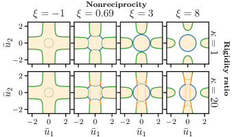
Figure 1: Linear stability thresholds for uniform steady states in the plane of mean concentrations for the NRCH model for increasing nonreciprocity parameter $\xi=\alpha^{2}-\rho^{2}$ (left to right) as well as equal ($\kappa=1$, top row) and unequal ($\kappa=20$) rigidity, i.e., without and with a conserved Turing instability, respectively. Further, $a=-1.5$. Linear instability is indicated by orange shading. Green, orange and blue thick [thin] lines indicate primary [secondary] Cahn-Hilliard, conserved Turing and conserved Hopf instabilities, respectively.

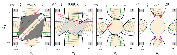
Figure 2: Phase diagrams in the ($\bar{u}_{1},\bar{u}_{2}$)-plane for the NRCH model for increasing nonreciprocity parameter $\xi=\alpha^{2}-\rho^{2}$ (left to right) as well as (a)-(c) equal ($\kappa=1$) and (d) unequal ($\kappa=20$) rigidity. For coexisting uniform phases, solid black and gray lines represent (stable and metastable) binodals and corresponding tie lines, respectively. Purple lines in (d) represent binodals for the coexistence of a uniform and a crystalline phase (tie lines are pink). Dashed black lines indicate unstable binodals, i.e., the coexisting state is linearly unstable. The dark [light] gray area in (a) [(b)] marks a stable [unstable] three-phase coexistence region. The white areas in the four corners are single phase regions, e.g., at the top left of the $\downarrow\uparrow$-phase (low $u_{1}$, high $u_{2}$). The spinodals are colored as in Fig. 1. Remaining parameters are $\rho=1$ and $a=-1.5$. The red lines indicate tie lines that are further analyzed in Figs. 3 to 5 and in section S3 of the SM as indicated.

As Eqs. (2) are conservation laws, they are solved by any uniform steady state $(u_{1},u_{2})=(\bar{u}_{1},\bar{u}_{2})$. However, these states may be unstable with respect to small perturbations. A linear stability analysis [9, 10, 18] gives the thresholds (spinodals) shown in Fig. 1. Following [10], we distinguish a Cahn-Hilliard (large-scale stationary), a conserved-Hopf (large-scale oscillatory), and a conserved-Turing (small-scale stationary) instability. The first is well known from phase separation in passive systems, but the latter two only occur for dominant nonreciprocity, i.e., for $\xi>0$. In analogy to usual two-species reaction-diffusion (RD) systems the Turing instability only occurs for unequal rigidities ($\kappa\neq 1$) that take the role diffusion constants have in RD systems, for details see [18].

At first sight, one might assume that coexisting states (binodals) can only be obtained via a Maxwell construction in the passive case, i.e., with completely reciprocal coupling (${\alpha=0}$) where Eqs. (2) still corresponds to a proper gradient dynamics. However, this can be achieved even for the case of Eqs. (2) with nonreciprocal coupling ($\alpha\neq 0$), i.e., for a broken gradient dynamics structure: Introducing an amended formal energy and mobility matrix as

$$\begin{split}\tilde{\mathcal{F}}&=\frac{\rho}{\rho+\alpha}\mathcal{F}_{1}+\frac{\rho}{\rho-\alpha}\mathcal{F}_{2}+\mathcal{F}_{\mathrm{12}}\\ \text{and}\quad\bm{\underline{\tilde{M}}}&=\begin{pmatrix}\frac{\rho+\alpha}{\rho}&0\\ 0&\frac{\rho-\alpha}{\rho}\end{pmatrix},\end{split}$$ (3)

respectively, Eqs. (2) can be written in the form of Eq. (1). This directly implies that one may use a Maxwell construction on $\tilde{\mathcal{F}}$ to obtain coexisting states and, in consequence, phase diagrams. However, one needs to take into account that for $\xi>0$ one solely has obtained a spurious gradient dynamics [17] as for dominating nonreciprocity $\tilde{\mathcal{F}}$ is not bounded from below and $\bm{\underline{\tilde{M}}}$ is not positive definite, i.e., basic thermodynamic principles are not fulfilled. As a result, the system may not approach an equilibrium, i.e., persistent oscillatory behavior may occur, implying that the spurious Maxwell construction, although powerful, only provides part of the picture.

The binodals for two coexisting phases A and B are determined via

$$\tilde{\mu}_{1}(\bm{u}^{(A)}) =\tilde{\mu}_{1}(\bm{u}^{(B)}),\quad\tilde{\mu}_{2}(\bm{u}^{(A)})=\tilde{\mu}_{2}(\bm{u}^{(B)})$$

$$\quad\text{and}\quad\tilde{p}(\bm{u}^{(A)}) =\tilde{p}(\bm{u}^{(B)}),$$ (4)

where $\bm{u}^{(A)}$ and $\bm{u}^{(B)}$ are the respective concentrations, the chemical potentials are $\tilde{\mu}_{i}=\partial\tilde{f}/\partial u_{i}$ with $\tilde{f}=\frac{\rho}{\rho+\alpha}f_{1}+\frac{\rho}{\rho-\alpha}f_{2}+f_{12}$, and the pressure is $\tilde{p}=\tilde{\mu}_{1}u_{1}+\tilde{\mu}_{2}u_{2}-\tilde{f}$. A derivation as well as the generalization for spatially periodic (crystalline) phases and a discussion of how the Maxwell approach developed in Ref. [16] for AMB can be accommodated is given in sections S1 and S5 of the Supplementary Material (SM). The resulting binodals we obtain by numerical continuation [24].

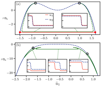
Figure 3: Bifurcation diagrams are given in terms of the pressure $\tilde{p}$ over $\bar{u}_{1}$ for $\alpha=0$ (reciprocal limit) for a finite domain size ($L=20\pi$). Panels (a) and (b) show the behavior along the two tie lines [(a) $\bar{u}_{2}=\bar{u}_{1}-0.151$ and (b) $\bar{u}_{2}=1.116\,\bar{u}_{1}+1.153$] marked in Fig. 2(a). Blue [green] lines correspond to branches of uniform [phase-separated] states while solid [dashed] lines indicate stability [instability]. Circles mark pitchfork bifurcations, and insets show typical concentration profiles for two- and three-phase coexistence.

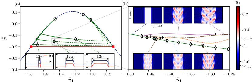
Figure 4: (a) Bifurcation diagram in terms of the (mean) pressure $\bar{\tilde{p}}$ over $\bar{u}_{1}$ along a path through Fig. 2(c) that corresponds to the marked tie line [$\bar{u}_{2}=1.116\bar{u}_{1}+1.081$]. Branches of uniform and phase-separated states are given as blue and green lines, respectively. For the latter, curves are shown for three domain sizes $L=20\pi,40\pi$ and $160\pi$ (top to bottom). Insets give the profiles at the Hopf bifurcations on the three branches for different $L$. (b) Magnification of the branch of stationary phase-separated states for $L=40\pi$ including more Hopf bifurcations than (a) and the first emerging branches of time-periodic states. The insets show corresponding space-time plots indicating the different localized oscillatory states (two periods are shown). Solid [dashed] lines indicate linearly stable [unstable] states. Circles [diamonds] mark Cahn-Hilliard [conserved-Hopf] instabilities. Small diamonds in (b) indicate torus bifurcations, i.e. Hopf bifurcations of limit cycles.

The obtained spinodals and binodals are combined into phase diagrams, as presented in Fig. 2(a) for the reciprocal case and in Fig. 2(b)-(d) for nonreciprocal cases of increasing $\xi$. The reciprocal case that is extensively analyzed elsewhere [9] allows for five two- and two three-phase coexistences of the four uniform phases characterized by the arrows in the four corners (e.g., $\uparrow\downarrow$ indicates high $u_{1}$ and low $u_{2}$). The bifurcation structure along the two highlighted lines in Fig. 2(a) is given in Fig. 3 in terms of the pressure $\tilde{p}$ and consists of branches of uniform and phase-separated states. For two-phase [three-phase] coexistence, Fig. 3(a) [Fig. 3(b)] follows a tie line [crosses a triple point region]. Although the considered domain is not very large (see insets), Fig. 3(a) nicely indicates how the Maxwell line (in red) is approached (cf. [21]) and all insets of Fig. 3 show the step-like fronts between phases.

The nonreciprocal cases in Fig. 2(b)-(d) do not show the field exchange symmetry ($u_{1}\leftrightarrow u_{2}$) of Fig. 2(a) as $\alpha\neq 0$, however field inversion [$(u_{1},u_{2})\leftrightarrow(-u_{1},-u_{2})$] is retained. The outer regions where at least one $|u_{i}|$ is large, are qualitatively as in Fig. 2(a) as the nonlinear parts of the $f_{i}$ dominate. Changes are strongest in the central region of low $|u_{i}|$. In Fig. 2(b) ($\xi=0.69$) the three-phase coexistence has become unstable as the coexisting phase of lowest $|u_{i}|$ has crossed the conserved-Hopf threshold. Further, the stable coexistence of $\downarrow\downarrow$- and $\uparrow\uparrow$-phase has disappeared. Bifurcation diagrams along the marked tie lines in Fig. 2(b) and corresponding concentration profiles with nonmonotonic front profiles are discussed in section S3 of the SM.

Then, at larger nonreciprocity ($\xi=3$), see Fig. 2(c), the four binodals have entirely separated from each other, triple point region and $\downarrow\downarrow$-$\uparrow\uparrow$ coexistence have disappeared, and the Hopf instability threshold now forms a closed curve and renders part of the binodals unstable. This results in a formal coexistence of a stable and an oscillatory unstable uniform state. Consequences for the bifurcation diagram are dramatic as can be appreciated in Fig. 4 (a). It follows the marked tie line in Fig. 2 (c). Now, the binodal at small $|u_{i}|$ is located in the central region where the $\downarrow\uparrow$-phase is Hopf-unstable. Again, a branch of phase-separated states (green, shown for three different domain sizes $L$) emerges from the branch of uniform states (blue) at the spinodals, undergoes saddle-node bifurcations (on the left and on the right). For large domains the almost horizontal central part again approaches the Maxwell line as for a reciprocal system. However, in stark contrast, here, when increasing $\bar{u}_{1}$ the phase-separated state becomes oscillatory unstable at a secondary Hopf bifurcation. For all considered $L$ this occurs when the unstable $\downarrow\uparrow$-phase has grown to an extend of $\approx 12\pi$ [insets of Fig. 4(a)], i.e., for larger $L$ it moves towards smaller $\bar{u}_{1}$. More such bifurcations follow and result in the emergence of several branches of time-periodic states, as shown in Fig. 4(b). Intriguingly, this results in the stable coexistence of a uniform $\downarrow\downarrow$-phase with an oscillatory $\downarrow\uparrow$-phase that is strictly confined to a region defined by the lever rule (branch in Fig. 4(b) that bifurcates supercritically at $\bar{u}_{1}\approx-1.47$, and eventually destabilizes at a Torus bifurcation). Additional windows of stability exist for other branches and are discussed together with corresponding time-simulations in section S4 of the SM. For large domains, we observe intricate irregular oscillatory motion that coexists with a stable uniform phase and is confined by stable domain boundaries.

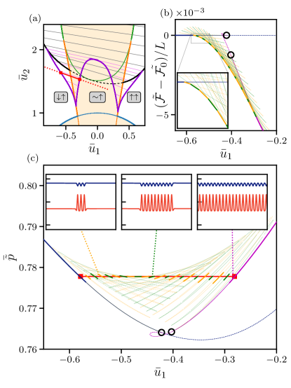
Figure 5: Panel (a) magnifies part of Fig. 2(d) focusing on the coexistence region of uniform and crystalline phases. Panels (b) and (c) analyze the bifurcation structure along the red tie line in (a) providing mean energy and pressure $\bar{\tilde{p}}$ over $\bar{u}_{1}$, respectively, Shown are uniform (blue), periodic (magenta), and even/odd (green/yellow) localized states, i.e., crystallites. Panels (b) and (c) highlight the states of lowest energy as piecewise thick lines, thereby in (c) illustrating how the Maxwell line (red horizontal) is approached. Parameters are as in Fig. 5 (d) and $L=80\pi$.

Further increasing $\xi$ entirely separates the binodals from the inner Hopf-unstable region [Fig. 2(d)]. In contrast to the previous cases, Fig. 2(d) considers unequal rigidities ($\kappa\neq 1$) allowing for a conserved-Turing instability. This directly results in the existence of crystalline phases and, in consequence, in four pairs of binodals (purple lines) that represent their coexistence with uniform phases. Such a region is magnified in Fig. 5(a). Following the binodals with increasing $|\bar{u}_{2}|$, the period of the involved crystalline states increases and finally diverges at $(\bar{u}_{1},\bar{u}_{2})\approx(0,1.9)$ (not shown). In other words, the crystalline phase transforms into a phase-separated state corresponding to the tangential convergence of the outer line of the uniform-crystal binodal (purple) onto the binodal for standard phase separation (black). In contrast, when decreasing $|\bar{u}_{2}|$ the coexistence ranges shrink till they terminate in cusps that represent tricritical points where the phase transition changes from first to second order (not very far from the Hopf threshold). The involved bifurcation structure along the red tie line in Fig. 5(a) is presented in Figs. 5(b) and 5(c) in terms of mean energy and pressure as a function of $\bar{u}_{1}$ ($\bar{u}_{2}=-0.353\,\bar{u}_{1}+1.431$). Overall, the behavior of this strongly nonreciprocal system indeed resembles the one known from passive phase-field-crystal (PFC) models [25, 26, 21]: Where the uniform state (stable at small $\bar{u}_{1}$) undergoes the conserved-Turing instability, a branch of periodic (crystalline) states emerges, itself soon spawning two branches of localized states that build up a “snakes and ladders” bifurcation structure (known as homoclinic snaking [27, 28, 29]). The snaking results in a large parameter range of multistability that overall represents phase coexistence. Figs. 5(b) and (c) highlight as heavy lines the states that correspond to the minima of the energy $\tilde{\mathcal{F}}$, i.e., pieces of the branches of uniform, crystalline and various localized states. Then, Fig. 5(c) reveals that, as shown in Ref. [21] for the passive PFC model, also for the NRCH model the piecewise curve defines a narrow horizontal band centered about the coexistence pressure. With increasing domain size the band will become smaller and approach the Maxwell line.

In other words, even for the considered linearly coupled NRCH model where crystalline states only emerge due to nonreciprocity, analyses based on equilibrium considerations can be applied when combined with further stability considerations.

In the present work, we have analyzed the direct application of aspects of equilibrium thermodynamics to a subclass of models for active systems, namely, models that can be transformed into a spurious gradient dynamics as defined in [17]. In particular, we have shown at the example of a linearly coupled two-field NRCH model for a ternary mixture with species-wise mass conservation that its nonequilibrium phase behavior is captured by a (spurious) Maxwell construction. This has allowed us to determine phase diagrams valid in the thermodynamic limit and to show that the Maxwell construction emerges from finite-domain bifurcation diagrams in overall similar ways to the known reciprocal cases [21]. This includes the case of crystalline states that for the NRCH model only emerge due to nonreciprocity and their coexistence with uniform states. However, as the underlying system is nonreciprocal also oscillatory modes may occur, e.g., resulting from the conserved-Hopf instability of uniform states [18, 10]. Intriguingly, we have found that the Maxwell construction may still be used to predict the coexistence of uniform and oscillatory states.

Our analysis of the specific NRCH model already indicates the validity of the approach for other models in the class of spurious gradient dynamics [17], like active PFC models [30, 31, 32], coupled Cahn-Hilliard and Swift-Hohenberg models [17], and the FitzHugh-Nagumo reaction-diffusion model [33]. These could all be (re-)investigated defining corresponding nonequilibrium chemical potentials $\tilde{\mu}_{i}$ and pressures $\tilde{p}$. The resulting Maxwell construction may then be employed to further elucidate the interplay of conservation laws and nonreciprocity.

References

- Cahn and Hilliard [1959] J. W. Cahn and J. E. Hilliard, Free energy of a nonuniform system. 3. Nucleation in a 2-component incompressible fluid, J. Chem. Phys. 31, 688 (1959).
- Hohenberg and Halperin [1977] P. C. Hohenberg and B. I. Halperin, Theory of dynamic critical phenomena, Rev. Mod. Phys. 49, 435 (1977).
- Clerk-Maxwell [1875] J. Clerk-Maxwell, On the dynamical evidence of the molecular constitution of bodies, Nature 11, 357 (1875).
- Dinelli et al. [2023] A. Dinelli, J. O’Byrne, A. Curatolo, Y. Zhao, P. Sollich, and J. Tailleur, Non-reciprocity across scales in active mixtures, Nat. Commun. 14, 10.1038/s41467-023-42713-5 (2023).
- Cates and Tailleur [2015] M. E. Cates and J. Tailleur, Motility-induced phase separation, Annu. Rev. Condens. Matter Phys. 6, 219 (2015).
- te Vrugt et al. [2023] M. te Vrugt, J. Bickmann, and R. Wittkowski, How to derive a predictive field theory for active brownian particles: a step-by-step tutorial, J. Phys.: Condens. Matter 35, 313001 (2023).
- Saha et al. [2020] S. Saha, J. Agudo-Canalejo, and R. Golestanian, Scalar active mixtures: The non-reciprocal Cahn-Hilliard model, Phys. Rev. X 10, 041009 (2020).
- You et al. [2020] Z. H. You, A. Baskaran, and M. C. Marchetti, Nonreciprocity as a generic route to traveling states, Proc. Natl. Acad. Sci. U. S. A. 117, 19767 (2020).
- Frohoff-Hülsmann et al. [2021] T. Frohoff-Hülsmann, J. Wrembel, and U. Thiele, Suppression of coarsening and emergence of oscillatory behavior in a Cahn-Hilliard model with nonvariational coupling, Phys. Rev. E 103, 042602 (2021).
- Frohoff-Hülsmann and Thiele [2023] T. Frohoff-Hülsmann and U. Thiele, Nonreciprocal cahn-hilliard model emerges as a universal amplitude equation, Phys. Rev. Lett. 131, 107201 (2023).
- Bergmann et al. [2018] F. Bergmann, L. Rapp, and W. Zimmermann, Active phase separation: a universal approach, Phys. Rev. E 98, 020603 (2018).
- Rapp et al. [2019] L. Rapp, F. Bergmann, and W. Zimmermann, Systematic extension of the Cahn-Hilliard model for motility-induced phase separation, Eur. Phys. J. E 42, 57 (2019).
- Wittkowski et al. [2014] R. Wittkowski, A. Tiribocchi, J. Stenhammar, R. J. Allen, D. Marenduzzo, and M. E. Cates, Scalar field theory for active-particle phase separation, Nat. Commun. 5, 4351 (2014).
- Tjhung et al. [2018] E. Tjhung, C. Nardini, and M. E. Cates, Cluster phases and bubbly phase separation in active fluids: reversal of the Ostwald process, Phys. Rev. X 8, 031080 (2018).
- Bickmann and Wittkowski [2020] J. Bickmann and R. Wittkowski, Collective dynamics of active Brownian particles in three spatial dimensions: A predictive field theory, Phys. Rev. Res. 2, 033241 (2020).
- Solon et al. [2018] A. P. Solon, J. Stenhammar, M. E. Cates, Y. Kafri, and J. Tailleur, Generalized thermodynamics of phase equilibria in scalar active matter, Phys. Rev. E 97, 020602 (2018).
- Frohoff-Hülsmann et al. [2023] T. Frohoff-Hülsmann, M. P. Holl, E. Knobloch, S. V. Gurevich, and U. Thiele, Stationary broken parity states in active matter models, Phys. Rev. E 107, 10.1103/physreve.107.064210 (2023).
- Frohoff-Hülsmann et al. [2023] T. Frohoff-Hülsmann, U. Thiele, and L. M. Pismen, Non-reciprocity induces resonances in a two-field cahn-hilliard model, Philos. Trans. R. Soc. A-Math. Phys. Eng. Sci. 381, 10.1098/rsta.2022.0087 (2023).
- Frohoff-Hülsmann and Thiele [2021] T. Frohoff-Hülsmann and U. Thiele, Localised states in coupled Cahn-Hilliard equations, IMA J. Appl. Math. 86, 924 (2021).
- Brauns and Marchetti [2023] F. Brauns and M. C. Marchetti, Non-reciprocal pattern formation of conserved fields, arxiv (2023), 2306.08868v3 .
- Thiele et al. [2019] U. Thiele, T. Frohoff-Hülsmann, S. Engelnkemper, E. Knobloch, and A. J. Archer, First order phase transitions and the thermodynamic limit, New J. Phys. 21, 123021 (2019).
- Cahn and Hilliard [1958] J. W. Cahn and J. E. Hilliard, Free energy of a nonuniform system. 1. Interfacial free energy, J. Chem. Phys. 28, 258 (1958).
- Cahn [1965] J. W. Cahn, Phase separation by spinodal decomposition in isotropic systems, J. Chem. Phys. 42, 93 (1965).
- Holl et al. [2021a] M. P. Holl, A. J. Archer, and U. Thiele, Efficient calculation of phase coexistence and phase diagrams: Application to a binary phase-field crystal model, J. Phys.: Condens. Matter 33, 115401 (2021a).
- Emmerich et al. [2012] H. Emmerich, H. Löwen, R. Wittkowski, T. Gruhn, G. I. Tóth, G. Tegze, and L. Gránásy, Phase-field-crystal models for condensed matter dynamics on atomic length and diffusive time scales: an overview, Adv. Phys. 61, 665 (2012).
- Thiele et al. [2013] U. Thiele, A. J. Archer, M. J. Robbins, H. Gomez, and E. Knobloch, Localized states in the conserved Swift-Hohenberg equation with cubic nonlinearity, Phys. Rev. E 87, 042915 (2013).
- Burke and Knobloch [2006] J. Burke and E. Knobloch, Localized states in the generalized Swift-Hohenberg equation, Phys. Rev. E 73, 056211 (2006).
- Knobloch [2016] E. Knobloch, Localized structures and front propagation in systems with a conservation law, IMA J. Appl. Math. 81, 457 (2016).
- Holl et al. [2021b] M. P. Holl, A. J. Archer, S. V. Gurevich, E. Knobloch, L. Ophaus, and U. Thiele, Localized states in passive and active phase-field-crystal models, IMA J. Appl. Math. 86, 896 (2021b).
- Menzel and Löwen [2013] A. M. Menzel and H. Löwen, Traveling and resting crystals in active systems, Phys. Rev. Lett. 110, 055702 (2013).
- Ophaus et al. [2018] L. Ophaus, S. V. Gurevich, and U. Thiele, Resting and traveling localized states in an active phase-field-crystal model, Phys. Rev. E 98, 022608 (2018).
- te Vrugt et al. [2022] M. te Vrugt, M. P. Holl, A. Koch, R. Wittkowski, and U. Thiele, Derivation and analysis of a phase field crystal model for a mixture of active and passive particles, Modelling Simul. Mater. Sci. Eng. 30, 084001 (2022).
- Schütz et al. [1995] P. Schütz, M. Bode, and H. G. Purwins, Bifurcations of front dynamics in a reaction-diffusion system with spatial inhomogeneities, Physica D 82, 382 (1995).
- Kuwamura and Yanagida [2003] M. Kuwamura and E. Yanagida, The Eckhaus and zigzag instability criteria in gradient/skew-gradient dissipative systems, Physica D 175, 185 (2003).