Bruno Buonomo^1,∗, Eleonora Messina^1,∗, Claudia Panico^1,∗, Antonia Vecchio^2,∗

¹ Department of Mathematics and Applications, University of Naples Federico II,
via Cintia, I-80126 Naples Italy.
²National Research Council of Italy, Institute for Computational Application ``M. Picone'',
Via P. Castellino, 111 - I-80131 Naples, Italy.

Abstract

We propose an integral model describing an epidemic of an infectious disease. The model is behavioural in the sense that the constitutive law for the force of infection includes a distributed delay, called information index, that describes the opinion-driven human behavioural changes. The information index, in turn, contains a memory kernel to mimic how the individuals maintain memory of the past values of the infection. We obtain sufficient conditions for the endemic equilibrium to be locally stable. In particular, we show that when the infectivity function is represented by an exponential distribution, stability is guaranteed by the weak Erlang memory kernel. However, through numerical simulations, we show that self-sustained oscillations may arise when the memory is more focused in the disease's past history, as exemplified by the strong Erlang kernel. We also show the model solutions in cases of different infectivity functions describing infectious diseases like influenza and SARS.

Keywords: mathematical epidemiology, renewal equations, stability, information, human behaviour

1 Introduction

Models of Mathematical Epidemiology (ME) have proved to be an effective tool for understanding epidemic dynamics and for identifying the best intervention and mitigation strategies. Many noteworthy cases can be cited where models of ME have been applied to recent diseases and parametrized with official data. Clear examples are the recent COVID-19 pandemic [17, 27, 29, 42], the transmission of Middle East Respiratory Syndrome (MERS) in South Korea and Saudi Arabia [46], and the spread of the West Nile virus in Italy [28].

In all of the above-mentioned cases, compartmental models were used in which the individuals of a given population were divided in mutually exclusive groups (the compartments) according to their respective disease status. Although compartmental models applied to real epidemics often have a complex structure, they are in fact extensions of minimal epidemic models. By `minimal', we mean models with a reduced mathematical complexity where the epidemic is described through slight variants of the basic SIR (Susceptible–Infectious–Removed) or SEIR (Susceptible–Exposed–Infectious–Removed) models. Study of these minimal models have attracted the attention of researchers for many years and may prove critical as paradigmatic models of specific dynamical outcomes such as bifurcations, hysteresis and oscillations [15, 16, 38]. It is well known that the minimal compartmental models refer back to the work of Kermack and McKendrick. In 1927, they published a celebrated paper in which an integral renewal equation (i.e. a model for epidemic propagation based on the individual infectiousness) was introduced [31] (see also the reprint [32]). Many researchers have made substantial contributions to the development of integral epidemic models in the field of epidemiology. An in-depth coverage of integral models in the mathematical modeling of infectious diseases can be found in current classical books on ME [7, 19]. Applications of integral epidemic models to actual diseases, such as influenza and Severe Acute Respiratory Syndrome (SARS), were provided by M. G. Roberts and coworkers [44, 45]. O. Diekmann and coworkers proposed mathematical formulations for a wide range of epidemic models that incorporate demography and non-permanent immunity as a scalar renewal equation for the Force of Infection (FoI), i.e. the rate at which a susceptible becomes infected [9]. In such a paper, the concept is introduced of infectivity function, which represents the expected contribution to the FoI by an individual infected since $\tau$ units of time. Kermack and McKendrick’s integral renewal equation reduces to classical models, such as SIR and SEIR, when the infectivity function assumes specific forms [18, 21].

Both renewal equations and compartmental models of ME do exhibit a notable limitation, however, that in many cases cannot be disregarded: they do not take into account the feedback effects produced by the behavioural change of individuals during an epidemic. Classical compartmental models have been revisited in recent years within the framework of a new field called Behavioural Epidemiology of Infectious Disease (BEID) [37, 50]. Among the possible approaches within the BEID, the one based on the so-called information index (i.e. a distributed delay which describes the opinion-driven changes of behaviour of individuals) is particularly promising and increasingly used [2, 33, 35]. The first studies on minimal epidemic models embedding the information index date back to 2007 with A. d'Onofrio and coworkers [25]. Generally speaking, scholars working on models of BEID focus on potential complex dynamics caused by the presence of behavioural effects. For example, it has been proven that the opinion-driven change of behaviour, modeled through the information index, can induce oscillatory dynamics that go uncaptured by analogous non-behavioural models [22, 25, 37, 50]. A key factor in the occurrence of oscillations is the type of memory kernel (i.e. the function used to model how a population keeps memory of information and rumours regarding a disease [22, 24, 25]). Recently, minimal epidemic models, including the information index, have been extended to incorporate more complex models for the study of vaccine hesitancy [12] and to obtain the value of the information-related parameters by using official data released by public health authorities [10, 11]. It is worth mentioning that in several papers, an awareness variable is employed to represent behavioural responses due to information. Such a variable can be considered as a special case of the information index [34, 47, 52].

In this paper, motivated by the recent promising advances of BEID, we offer a new contribution to the theory of integral renewal equations in ME. We propose a behavioural renewal equation where the FoI incorporates the information index and the model therefore takes into account human behavioural feedback. As far as we know, this is the first investigation on integral renewal equations that embed the information index.

Our approach provides a qualitative analysis of the model based on stability theory. That is, we obtain sufficient conditions for the endemic equilibrium to be locally stable. Such conditions are written in terms of the memory kernel, the infectivity function and the so-called message function, which describes the information that forms the opinion of individuals. Moreover, through numerical simulations based on a non-standard method, we show how the memory kernel affects the dynamical outcomes of the model. We also show the model solutions in case of some different infectivity functions describing infectious diseases, like Influenza and SARS. Since the renewal equation is a generalization of epidemic models ruled by Ordinary Differential Equations (ODEs), this study also extends the results concerning the minimal behavioural models to more general (and potentially more realistic) cases.

The paper is organized as follows: in Section 2, we introduce the constitutive equation for the FoI incorporating human behavioural feedback. We also describe the renewal equation model in detail. Section 3 focuses on the basic properties of the solution, including positivity and boundedness. We prove that the system admits two equilibria under specific assumptions. In Section 4, we derive the characteristic equation as a preliminary for the stability analysis. Section 5 is devoted to the local stability analysis of the equilibria. In Section 6, we shortly discuss the non-standard method built for the problem at hand and show some applications using infectivity functions proposed for specific infectious diseases. Finally, conclusions and future prospectives are provided in Section 7.

2 The behavioural renewal equation

In the formulation of the Kermack and McKendrick's integral renewal equation [9], the FoI at time $t$, denoted by $F(t)$, is introduced through the following constitutive equation:

$$F(t)=\int_{0}^{\infty}S(t-\tau)F(t-\tau)A_{\mu}(\tau)d\tau.$$ (1)

Here, $S$ denotes the size of the susceptible compartment and $A_{\mu}$ is the Infectivity Function with Demography (IFD). The IFD is defined as $A_{\mu}(\tau)=e^{-\mu\tau}A(\tau)$, where $e^{-\mu\tau}$ represents the probability that an individual stays alive for at least $\tau$ units of time; $\mu$ is the per capita natural death rate and $A(\tau)$ is the Infectivity Function (IF). The IF is defined as the expected contribution to the force of infection by an individual that was itself infected $\tau$ units of time ago. It is assumed to be an $L^{1}$ function from $[0,\infty)$ to $[0,\infty)$.

It is well known that compartmental models can be derived from the renewal equation (1) (see [18, 21]). In this regard, a key role is played by the IF. For example, if $A(\tau)$ is an exponential function or a linear combination of exponential functions, from (1) one can derive the classical SIR and SEIR compartmental models ruled by three and four ODEs, respectively.

In the behavioural formulation of epidemic models based on the information index it is explicitly taken into account that the transmission of information and rumours about the disease are often preceded by articulated routine procedures so that public awareness regarding the disease takes time to build [37, 50]. Moreover, people keeps memory of the past values of the infection. Therefore, delay and memory are two major aspects of the opinion-driven change of behaviour. The information index, $M(t)$, summarizes these aspects and is defined as the following distributed delay:

$$M(t)=\int_{0}^{\infty}H(t-\tau)\,g\big{(}x_{1}(t-\tau),x_{2}(t-\tau),\dots,x_{n}(t-\tau)\big{)}\,K(\tau)\,d\tau,$$

where $H(\cdot)$ is the Heaviside step function and

• the quantities $x_{1},x_{2},\dots,x_{n}$ are the state variables of the epidemic model under consideration;

• the message function $g$ describes the individuals' perceived risks associated to the disease. In principle, it may depend on all the state variables, but, in practice, it is assumed to depend only on some specific quantities as, for example, the incidence and the prevalence of the disease;

• $K(\cdot)$ is the memory kernel, such that $K(t)>0$ and $\int_{0}^{\infty}K(t)dt=1$. For example, the memory kernel can be chosen to be a Dirac delta $K(t)=\delta(t)$, which represents the instantaneous propagation of the information, or an Erlang distribution with rate parameter $a$ and shape parameter $n$,

  $$K(t)=Erl_{n,a}(t)=\frac{a^{n}}{(n-1)!}t^{n-1}e^{-nt},\quad a\in\mathbb{R^{+}},\quad n\in\mathbb{N^{+}},$$

  which includes both the cases of unimodal kernels (when $n>1$) and of exponentially fading memory (when $n=1$) in which the memory of the mean individual decays with characteristic length $T=1/a$, see [37, 50].

Now we propose the following variation of the constitutive law (1) for the FoI

$$F(t)=\int_{0}^{\infty}\beta\big{(}M(t-\tau)\big{)}S(t-\tau)F(t-\tau)A_{\mu}(\tau)d\tau.$$ (2)

Here, the function $\beta(M)$ describes the inhibitory contribution to the FoI due to the information and rumours regarding the disease status. It is reasonable to assume that: $\beta(M)>0$, $\beta(0)=1$ and $\beta^{\prime}(M)<0$. In the context of the renewal equation formulation, we propose that the message function $g$ depends on the FoI and set

$$M(t)=\int_{0}^{\infty}H(t-\tau)g\big{(}F(t-\tau)\big{)}\,K(\tau)\,d\tau,$$ (3)

where $g(0)=0$, $g(F)\geq 0$ and $g^{\prime}(F)>0$. Denoting by $\lambda$ the net inflow of susceptibles in the population, the balance equation for the susceptibles is given by

$$\dot{S}(t)=\lambda-\mu S(t)-\beta(M(t))S(t)F(t),$$ (4)

where the upper dot denotes the time derivative and $F(t)$ is defined through the constitutive equation (2). Collecting together (2), (3) and (4), the complete model reads

$$\dot{S}(t)=\lambda-\mu S(t)-\beta(M(t))S(t)F(t),$$ (5)

$$F(t)=\int_{0}^{\infty}\beta\big{(}M(t-\tau)\big{)}S(t-\tau)F(t-\tau)A_{\mu}(\tau)d\tau,$$

$$M(t)=\int_{0}^{\infty}H(t-\tau)g\big{(}F(t-\tau)\big{)}K(\tau)d\tau.$$

For the sake of clarity, we report in Table 1 the definition of the parameters and quantities related to model (5) and in Table 2 the assumptions on the functions involved in model (5), which we suppose to hold from now on.

Symbol	Meaning
$\lambda$	Net inflow of susceptibles
$\mu$	Natural death rate
$R_{0}$	Basic Reproduction Number
$N$	Total population size
$S_{0}$	Initial susceptible population

Table 1: Description of the parameters and quantities related to model (5). Note that $N=\lambda/\mu$.

Function	Meaning	Assumptions
$A$	Infectivity function	$A(t)\geq 0$
$A_{\mu}$	Infectivity function with demography	$\hat{A}_{\mu}(0):=\int_{0}^{\infty}A_{\mu}(t)dt<+\infty$
$\beta$	Inhibition function	$\beta(0)=1$, $\beta(M)>0$, $\beta^{\prime}(M)<0$
$g$	Message function	$g(0)=0$, $g(\cdot)\geq 0$, $g^{\prime}(\cdot)>0$
$K$	Memory kernel	$K(\tau)>0$, $\int_{0}^{\infty}K(\tau)d\tau=1$

Table 2: Functions involved in model (5) and the related assumptions.

We conclude the section by showing that the renewal equation model (5) is a generalization of behavioural compartmental models.

Proposition 2.1.

If the IF is exponentially distributed, then model (5) is the behavioural SIR–M model introduced in [22].

Proof.

Let us take $A(\tau)=\beta_{0}e^{-\nu\tau}$, where $\beta_{0}$ and $\nu$ are two positive constants representing the transmission rate and the average duration of the infectious period, respectively. Set

$$I(t)=\int_{0}^{\infty}e^{-(\mu+\nu)\tau}\beta(M(t-\tau))F(t-\tau)S(t-\tau)d\tau,$$

substitution of $A_{\mu}(\tau)=\beta_{0}e^{-(\mu+\nu)\tau}$ into equation (2) leads to $F(t)=\beta_{0}I(t)$. It follows:

$$\frac{dI(t)}{dt} =-(\mu+\nu)\int_{0}^{\infty}e^{-(\mu+\nu)\tau}\beta(M(t-\tau))F(t-\tau)S(t-\tau)d\tau+\beta(M(t))F(t)S(t)$$

$$=-(\mu+\nu)I(t)+\beta_{0}\beta(M(t))I(t)S(t).$$

By denoting $\hat{\beta}(M)=\beta_{0}\beta(M)$, then

$$\dot{I}=-(\mu+\nu)I+\hat{\beta}(M)SI.$$ (6)

Equations (3),(4) and (6) constitutes the extensively studied behavioural SIR–M model introduced by d'Onofrio et al [22]. ∎

Remark 2.1.

In the early epidemic model by Kermack and McKendrick [31, 32], it is assumed that factors such as infectivity, recovery, and mortality depend on the age-of-infection, i.e. the time elapsed by the infection. It is worth to mention that the infectious individuals may be further distinguished (say structured) according to their age-of-infection. This assumption lead to consider the age-of-infection as an independent variable and the corresponding models are integro-differential models involving partial differential equations. Time-since-infection (and time-since-recovery) structured epidemic models have been studied by several authors (see e.g. [26, 38]). A time-since-infection behavioural model has been recently studied, where the individuals' decisions regarding vaccination is driven by imitation dynamics [51].

3 Basic properties and existence of equilibria

In order to study the solution $\textbf{u}(t)=(S(t),F(t),M(t))$ of model (5), we assume that, over the interval $(-\infty,0]$, the state variables $S$, $F$ and $M$ are bounded functions and $0<S(t)\leq\lambda/\mu$, $F(t)\geq 0$, $M(t)\geq 0$. These properties hold true for all $t\in\mathbb{R}$, in view of the following two theorems.

Theorem 3.1.

The inequalities $S(t)>0$, $F(t)\geq 0$, $M(t)\geq 0$ hold true for all $t>0$.

Proof.

From the first equation of (5) we deduce that

$$S(t)=e^{-\int_{0}^{t}\left[\mu+\beta(M(\tau))F(\tau)\right]d\tau}\Big{(}S_{0}+\int_{0}^{t}\lambda e^{\int_{0}^{s}\left[\mu+\beta(M(\tau))F(\tau))\right]d\tau}ds\Big{)}.$$

Being $S(0)=S_{0}>0$, it easily follows that $S(t)>0$, $\forall t\geq 0$. The non-negativity of $F(t)$ and $M(t)$ follows from the non-negativity of the functions $A$, $\beta$, $g$ and $K$ (see the assumptions in Table 2). ∎

Theorem 3.2.

Assume that $A^{\prime}(\tau)\in L^{1}([0,\infty))$ and $\lim_{\tau\rightarrow\infty}A(\tau)=0,$ then $S(t)\leq S_{\max}$, $F(t)\leq F_{\max}$, $M(t)\leq M_{\max},$ for all $t>0$, where

$$S_{\max}=\frac{\lambda}{\mu},\quad F_{\max}=\lambda\hat{A}_{\mu}(0)+\frac{\lambda}{\mu}\int_{0}^{\infty}|A_{\mu}^{\prime}(\tau)|d\tau,\quad M_{\max}=g(F_{max}).$$ (7)

Proof.

The non-negativity of $S(t)$, $F(t)$ and $\beta(M(t))$ implies that $\dot{S}(t)\leq\lambda-\mu S(t)$. Thus, using the comparison theorem, we obtain

$$S(t) \leq e^{-\mu t}\left(S_{0}+\lambda\int_{0}^{t}e^{\mu s}ds\right)=\frac{\lambda}{\mu}+\left(S_{0}-\frac{\lambda}{\mu}\right)e^{-\mu t}.$$

Since $S_{0}\leq\lambda/\mu$, we obtain the first bound. From the first and the second equation in (5), we have

$$F(t) =\lambda\int_{0}^{\infty}A_{\mu}(\tau)d\tau-\mu\int_{0}^{\infty}S(t-\tau)A_{\mu}(\tau)d\tau-\int_{0}^{\infty}\dot{S}(t-\tau)A_{\mu}(\tau)d\tau.$$

Thus, since $\int_{0}^{\infty}S(t-\tau)A_{\mu}(\tau)d\tau\geq 0$, we deduce that

$$F(t)\leq\lambda\int_{0}^{\infty}A_{\mu}(\tau)d\tau-\int_{0}^{\infty}\dot{S}(t-\tau)A_{\mu}(\tau)d\tau.$$ (8)

Integrating by parts the second term in the r.h.s of (8), taking into account the non-negativity of the functions involved and that $\lim_{\tau\rightarrow\infty}A(\tau)=0$, we obtain the following bound for $F(t)$:

$$F(t) \leq\lambda\hat{A}_{\mu}(0)+\frac{\lambda}{\mu}\int_{0}^{\infty}|A_{\mu}^{\prime}(\tau)|d\tau,$$

where $\hat{A}_{\mu}(0):=\int_{0}^{\infty}A_{\mu}(\tau)d\tau$. Finally, from the third equation in (5), since $g$ is increasing and $\int_{0}^{\infty}K(\tau)d\tau=1$, we have

$$M(t)=\int_{0}^{\infty}H(t-\tau)g\big{(}F(t-\tau)\big{)}K(\tau)d\tau\leq g(F_{max})\int_{0}^{\infty}K(\tau)d\tau=g(F_{max}).$$

∎

The analysis of equilibria begins by observing that model (5) admits a unique Disease-Free Equilibrium (DFE) given by

$$DFE=(\bar{S}_{0},0,0),$$ (9)

where $\bar{S}_{0}=\lambda/\mu$. Denote by

$$EE=(S_{e},F_{e},M_{e}),$$ (10)

the generic Endemic Equilibrium (EE) of model (5), i.e. equilibria where $F_{e}>0$. Endemic equilibria are obtained from conditions

$$\begin{array}[]{ll}\lambda-\mu S-\beta(M)SF=0,\quad\beta(M)S\hat{A}_{\mu}(0)=1,\quad M=g(F).\end{array}$$ (11)

Introduce

$$R_{0}=\frac{\lambda}{\mu}\hat{A}_{\mu}(0).$$ (12)

Theorem 3.3.

If the assumptions of Theorem 3.2 hold, then: (i) if $R_{0}<1$, then model (5) has no endemic equilibria; (ii) if $R_{0}>1$, then model (5) has a unique endemic equilibrium.

Proof.

The EE is defined by the following conditions

$$M_{e}=g(F_{e}),\quad\quad S_{e}=\frac{\lambda}{\mu R_{0}\beta(g(F_{e}))},$$ (13)

and $F_{e}>0$ is the zero of the non linear function

$$G(x)=x-\mu R_{0}+\frac{\mu}{\beta(g(x))},$$ (14)

in the interval $[0,F_{max}]$, where $F_{\max}$ is introduced in (7). We observe that

$$G(0)=-\mu(R_{0}-1),$$

$$G(F_{max})=\lambda\int_{0}^{\infty}|A_{\mu}^{\prime}(\tau)|d\tau+\frac{\mu}{\beta(g(F_{max}))}>0,$$

$$G^{\prime}(x)=1-\frac{\mu\beta^{\prime}(g(x))g^{\prime}(x)}{[\beta(g(x))]^{2}\hat{A}_{\mu}(0)}>0,$$

where the last inequality holds since $\beta^{\prime}(\cdot)<0.$ Thus, when $R_{0}>1$, it is $G(0)<0$ and $G(x)$ in (14) has a unique zero in $[0,F_{\max}].$ Furthermore, if $R_{0}<1$, then $G(x)$ has no zeros in $[0,F_{max}].$

∎

Remark 3.1.

The quantity denoted by $R_{0}$ and introduced in (12) assumes the meaning of Basic Reproduction Number and it is an important indicator for analyzing the behaviour of epidemic models. In (12), $\hat{A}_{\mu}(0)$ represents the ability to generate secondary cases of infection from an individual within a population (in fact, if $A_{\mu}(\tau)=\beta_{0}e^{-(\mu+\nu)\tau}$, the quantity $\hat{A}_{\mu}(0)$ reduces to the transmission rate $\beta_{0}$ multiplied by the average infectious period $1/(\mu+\nu)$).

If $\hat{A}_{\mu}(0)$ is multiplied by the total population size $N=\lambda/\mu$, the meaning of $R_{0}$, that is the average number of secondary cases produced by one primary infection over the course of the infectious period in a fully susceptible population, is obtained.

4 Preliminaries for stability

In this section we derive the characteristic equation as preliminary step of the local stability analysis of the equilibria. We use the linearization theory for Volterra integral equations [41]. We begin by observing that model (5) can be written in integral form as

$$S(t) =S_{0}+\int_{0}^{t}\big{(}\lambda-\mu S(t-\tau)-\beta(M(t-\tau))S(t-\tau)F(t-\tau)\big{)}d\tau,$$

$$F(t) =F_{0}(t)+\int_{0}^{t}\beta(M(t-\tau))S(t-\tau)F(t-\tau)A_{\mu}(\tau)d\tau,$$ (15)

$$M(t) =M_{0}(t)+\int_{0}^{t}g(F(t-\tau))K(\tau)d\tau,$$

where the functions $F_{0}(t)$ and $M_{0}(t)$ are defined by

$$F_{0}(t) =\int_{t}^{\infty}\beta(M(t-\tau))S(t-\tau)F(t-\tau)A_{\mu}(\tau)d\tau,$$ (16)

$$M_{0}(t) =\int_{t}^{\infty}H(t-\tau)g(F(t-\tau))K(\tau)d\tau=g(F(0))K(t).$$

Consider the perturbations $(W,V,Z)$ to the generic equilibrium $\tilde{E}=(\tilde{S},\tilde{F},\tilde{M})$

$$S=\tilde{S}+W,\quad F=\tilde{F}+V,\quad M=\tilde{M}+Z.$$

Linearization of (4) about the equilibrium solution leads to the following system:

$$\textbf{y}(t)=\textbf{f}(t)+\int_{0}^{t}\mathcal{\textbf{Q}}(t-\tau)\textbf{y}(\tau)d\tau,$$ (17)

where

$$\textbf{y}(t)=\begin{bmatrix}W(t)\\ V(t)\\ Z(t)\end{bmatrix},\quad\textbf{f}(t)=\begin{bmatrix}W(0)\\ V_{0}(t)\\ Z_{0}(t)\end{bmatrix},$$

and

$$\mathcal{\textbf{Q}}(t)=\begin{bmatrix}-\mu-\beta(\tilde{M})\tilde{F}&-\beta(\tilde{M})\tilde{S}&-\beta^{\prime}(\tilde{M})\tilde{F}\tilde{S}\\ \beta(\tilde{M})\tilde{F}A_{\mu}(t)&\beta(\tilde{M})\tilde{S}A_{\mu}(t)&\beta^{\prime}(\tilde{M})\tilde{S}\tilde{F}A_{\mu}(t)\\ 0&K(t)g^{\prime}(\tilde{F})&0\end{bmatrix}.$$

Furthermore, the forcing terms are

$$V_{0}(t)=\int_{t}^{\infty}\bigg{[}\beta\big{(}M(t-\tau)\big{)}S(t-\tau)F(t-\tau)-\beta(\tilde{M})\tilde{S}\tilde{F}\bigg{]}A_{\mu}(\tau)d\tau,$$

$$Z_{0}(t)=\big{[}g(F(0))-g(\tilde{F})\big{]}K(t).$$

In order to study the stability of $\tilde{E}$, we refer to an extension of the classical Paley-Wiener theorem. This extension is recalled in Appendix B (Theorem B.1), to which we refer for the meaning of the symbols. System (17) fits into the form (35)-(36) with $l=1$, $k=2$, and

$$f_{0}(t) =W(0),$$

$$\textbf{{f}}_{1}(t) ={\small\begin{bmatrix}\displaystyle\int_{t}^{\infty}\big{[}\beta\big{(}M(t-\tau)\big{)}S(t-\tau)F(t-\tau)-\beta(\tilde{M})\tilde{S}\tilde{F}\big{]}A_{\mu}(\tau)d\tau\\ \big{[}g(F(0))-g(\tilde{F})\big{]}K(t)\end{bmatrix},}$$

$$\mathbf{A_{\infty}^{1}} =[-\mu-\beta(\tilde{M})\tilde{F},\quad-\beta(\tilde{M})\tilde{S},\quad-\beta^{\prime}(\tilde{M})\tilde{F}\tilde{S}].$$

Let $\hat{A}_{\mu}$ and $\hat{K}$ denote the Laplace transforms

$$\hat{A}_{\mu}(w)=\int_{0}^{\infty}e^{-wt}A_{\mu}(t)dt,\quad\hat{K}(w)=\int_{0}^{\infty}e^{-wt}K(t)dt,$$ (18)

with $w\in\mathbb{C}$. If $Re(w)>0$, the characteristic equation of system (17) takes the form

$$det\begin{bmatrix}w+\mu+\beta(\tilde{M})\tilde{F}&\beta(\tilde{M})\tilde{S}&\beta^{\prime}(\tilde{M})\tilde{F}\tilde{S}\\ -\beta(\tilde{M})\tilde{F}\hat{A}_{\mu}(w)&1-\beta(\tilde{M})\tilde{S}\hat{A}_{\mu}(w)&-\beta^{\prime}(\tilde{M})\tilde{S}\tilde{F}\hat{A}_{\mu}(w)\\ 0&-g^{\prime}(\tilde{F})\hat{K}(w)&1\end{bmatrix}=0.$$ (19)

Under the assumptions of Theorem 3.2, we have that the functions $f_{0}$ and $\textbf{{f}}_{1}$ satisfy the hypothesis of Theorem B.1. The following theorem gives a sufficient condition for the local asymptotic stability of the equilibria.

Theorem 4.1.

Any equilibrium $\tilde{E}=(\tilde{S},\tilde{F},\tilde{M})$ of model (5) is locally asymptotically stable if the characteristic equation

$$\beta(\tilde{M})\tilde{S}\hat{A}_{\mu}(w)\bigg{(}1+\frac{g^{\prime}(\tilde{F})\beta^{\prime}(\tilde{M})\tilde{F}\hat{K}(w)}{\beta(\tilde{M})}\bigg{)}=1+\frac{\beta(\tilde{M})\tilde{F}}{w+\mu},$$ (20)

has no solution for $Re(w)\geq 0$.

Proof.

(Sketch) The proof is a straightforward application of Theorem B.1, after observing that the transcendental equation (20) is equivalent to (19). ∎

We conclude the section by noting that the information dependent parameters affect the location of the equilibrium EE only through the message function (see the term $g(F_{e})$ in (13), (14)), while its stability properties depend also on the memory kernel $K$.

5 Local stability analysis of equilibria

In this section we analyze the stability properties of the equilibria DFE and EE, by applying Theorem 4.1 to some special cases of interest. In our analysis we assume that $Re(w)>0$. All the results can be easily extended to $Re(w)\geq 0$, by passing to the limit for $\tilde{w}\rightarrow w$ with $Re(\tilde{w})>0$.

At the DFE (9) the characteristic equation (20) simply reduces to $\bar{S}_{0}\hat{A}_{\mu}(w)=1$ and $Re(w)>0$ implies

$$\bigg{|}\frac{\lambda}{\mu}\hat{A}_{\mu}(w)\bigg{|}\leq\frac{\lambda}{\mu}\hat{A}_{\mu}(0).$$

Therefore, from Theorem 4.1 and (12) the DFE is locally asymptotically stable if $R_{0}<1$.

Regarding the equilibrium EE (10), from the characteristic equation (20) we obtain sufficient stability conditions in some specific cases. Generally speaking, the study of the roots of the characteristic equation is based on the following considerations: when $Re(w)>0$ it is

$$|\beta(M_{e})S_{e}\hat{A}_{\mu}(w)|\leq 1,\quad Re\bigg{(}1+\frac{\beta(M_{e})F_{e}}{w+\mu}\bigg{)}>1,$$ (21)

where the first inequality comes from condition (11)₂ and the second one is a direct consequence of $Re(w)>0$. Given (21), a sufficient condition guaranteeing that the characteristic equation (20) does not have roots $w$ such that $Re(w)\geq 0$ (as required by Theorem 4.1) is given by

$$\bigg{|}1+\frac{g^{\prime}(\tilde{F})\beta^{\prime}(\tilde{M})\tilde{F}\hat{K}(w)}{\beta(\tilde{M})}\bigg{|}\leq 1.$$ (22)

In the following, we discuss three noteworthy cases according to the form of the memory kernel $K$: no-delay; exponentially fading memory; unimodal memory.

Case (i): no-delay (Dirac's delta memory kernel, $K=\delta$). From (20) we get

$$g^{\prime}(F_{e})\beta^{\prime}(M_{e})F_{e}S_{e}\hat{A}_{\mu}(w)+\beta(M_{e})S_{e}\hat{A}_{\mu}(w)=1+\frac{\beta(M_{e})F_{e}}{w+\mu}.$$ (23)

Theorem 5.1.

If $K(\tau)=\delta(\tau)$ and $A_{\mu}(\tau)$ is a positive definite function, then EE is LAS for any choice of the functions $\beta$ and $g$.

Proof.

Let be $Re(w)>0$. For the Bochner characterization of positive definite functions (see Section 8.2 in [36]), it is $Re\big{(}\hat{A}_{\mu}(w)\big{)}\geq 0.$

Thus, in view of (21), since $g^{\prime}(\cdot)>0$ and $\beta^{\prime}(\cdot)<0$, the real part of the left-hand side of (23) is less than 1, while the real part of the r.h.s. is strictly greater than 1. Therefore equation (23) can never be satisfied. ∎

Remark 5.1.

An example of positive definite infectivity function is $A_{\mu}(\tau)=e^{-(\mu+\nu)\tau}$, for which model (5) is the $SIR-M$ model (4)-(6), as shown in Proposition 2.1. More generally, any non-negative, non-increasing infectivtiy function, convex on $[0,\infty)$, is positive definite [36] and thus Theorem 5.1 applies.

Theorem 5.2.

If $K(\tau)=\delta(\tau)$, $A^{\prime}(\tau)<0$, and the functions $\beta$ and $g$ are such that

$$g^{\prime}(F_{e})\beta^{\prime}(M_{e})F_{e}\leq-\beta(M_{e}),$$

then EE is LAS.

Proof.

Let be $\omega=x+iy$, with $x>0.$ We treat the three cases $y=0,$ $y>0,$ and $y<0$ separately.

• If $y=0,$ we consider equation (23) for which the inequalities (21) hold. Since in this case $g^{\prime}(F_{e})\beta^{\prime}(M_{e})F_{e}S_{e}\hat{A}_{\mu}(w)<0,$ for the assumptions on $\beta$ and $g$ in Table 2, the left-hand-side is less than one and cannot be equal to the r.h.s., which is in turn greater than one. So, equation (23) has no roots with positive real part.

• If $y>0,$ we write the imaginary part of equation (23) as

  $$\bigg{(}1+\frac{g^{\prime}(F_{e})\beta^{\prime}(M_{e})F_{e}}{\beta(M_{e})}\bigg{)}y\int_{0}^{\infty}e^{-xt}\sin(yt)A_{\mu}(t)dt=\frac{\beta(M_{e})F_{e}y^{2}}{(x+\mu)^{2}+y^{2}}.$$ (24)

  Inspired by the proof of [48, Lemma 1] we observe that, since, for the theorem assumption, $e^{-xt}A_{\mu}(t)$ is a strictly decreasing function, it is

  $$\int_{0}^{\infty}e^{-xt}\sin{(yt)}A_{\mu}(t)dt=\sum_{j=0}^{+\infty}\int_{\frac{2\pi j}{y}}^{\frac{2\pi(j+1/2)}{y}}(e^{-xt}A_{\mu}(t)-e^{-x(t+\pi/y)}A_{\mu}(t+\pi/y))\sin{(yt)}dt>0.$$

  It follows that

  $$y\int_{0}^{\infty}e^{-xt}\sin(yt)A_{\mu}(t)dt>0.$$

  The positivity of r.h.s. of (24) implies that the characteristic equation (23) can never be satisfied if

  $$1+\frac{g^{\prime}(F_{e})\beta^{\prime}(M_{e})F_{e}}{\beta(M_{e})}\leq 0.$$

• If $y=-z<0,$ then $\sin{(yt)}=-\sin{(zt)}$. This case is treated as the previous one since

  $$\int_{0}^{\infty}e^{-xt}\sin{(yt)}A_{\mu}(t)dt=-\int_{0}^{\infty}e^{-xt}\sin{(zt)}A_{\mu}(t)dt<0.$$

∎

Case (ii): exponentially fading memory (weak Erlang memory kernel, $K(\tau)=ae^{-a\tau}$). The Laplace transform in (18) reads $\hat{K}(w)=a/(a+w)$. Therefore, the sufficient condition (22) can be written as

$$\bigg{|}1+\frac{ag^{\prime}(F_{e})\beta^{\prime}(M_{e})F_{e}}{\beta(M_{e})(a+w)}\bigg{|}\leq 1.$$ (25)

Theorem 5.3.

If $K(\tau)=ae^{-a\tau}$ and the functions $\beta$ and $g$ satisfy the inequality

$$g^{\prime}(F_{e})\beta^{\prime}(M_{e})F_{e}\geq-2\beta(M_{e}),$$ (26)

then EE is LAS for any choice of $A_{\mu}(\tau)$.

Proof.

Let us set $w=x+iy$, with $x>0$, and $c=\frac{g^{\prime}(F_{e})\beta^{\prime}(M_{e})F_{e}}{\beta(M_{e})}$. It is

$$\bigg{|}1+\frac{ag^{\prime}(F_{e})\beta^{\prime}(M_{e})F_{e}}{\beta(M_{e})(a+w)}\bigg{|}^{2}=1+\frac{ca}{(a+x)^{2}+y^{2}}\bigg{(}ca+2(a+x)\bigg{)}.$$

Therefore, the sufficient condition (25) is satisfied if and only if

$$-1\leq\frac{ca}{(a+x)^{2}+y^{2}}\bigg{(}ca+2(a+x)\bigg{)}\leq 0.$$

Taking into account that $\beta^{\prime}(\cdot)<0$, this condition is always satisfied if $-c\leq 2$, which is equivalent to (26).

∎

Remark 5.2.

The result given in Theorem 5.3 remains valid in the no-delay case $K(\tau)=\delta(\tau)$. As matter of fact, the sufficient condition (22) turns out to be

$$\bigg{|}1+\frac{g^{\prime}(F_{e})\beta^{\prime}(M_{e})F_{e}}{\beta(M_{e})}\bigg{|}\leq 1,$$

which is equivalent to (26), since $\beta^{\prime}(M_{e})<0$.

Case (iii): unimodal memory (strong Erlang memory kernel, $K(\tau)=a^{2}\tau e^{-a\tau}$). The Laplace transform in (18) reads $\hat{K}(w)=\frac{a^{2}}{(a+w)^{2}}$. Therefore, the sufficient condition (22) is

$$\bigg{|}1+\frac{a^{2}g^{\prime}(F_{e})\beta^{\prime}(M_{e})F_{e}}{\beta(M_{e})(a+w)^{2}}\bigg{|}\leq 1.$$ (27)

Reasoning as in the proof of Theorem 5.3, let us set $w=x+iy$, with $x>0$, and $c=\frac{g^{\prime}(F_{e})\beta^{\prime}(M_{e})F_{e}}{\beta(M_{e})}$. It is

$$\bigg{|}1+\frac{\hat{K}(w)g^{\prime}(F_{e})\beta^{\prime}(M_{e})F_{e}}{\beta(M_{e})}\bigg{|}^{2} =1+2ca^{2}\frac{a^{2}((a+x)^{2}-y^{2})}{((a+x)^{2}+y^{2})^{2}}+\frac{c^{2}a^{4}}{((x+a)^{2}+y^{2})^{2}}.$$

Since $\beta^{\prime}(\cdot)<0$, it follows that (27) is satisfied if and only if

$$-1\leq 2ca^{4}\frac{((a+x)^{2}-y^{2})}{((a+x)^{2}+y^{2})^{2}}+\frac{c^{2}a^{4}}{((x+a)^{2}+y^{2})^{2}}\leq 0.$$

We observe that, while the left inequality is obviously accomplished, the right one can be written as

$$2(a+x)^{2}\geq-ca^{2}+2y^{2},$$

which is not true for any $w$ with $Re(w)\geq 0$, as required by Theorem 4.1. Therefore, instability of the equilibrium EE may take place in principle. In the next section, through numerical simulation, we will show that self-sustained oscillations may occur indeed.

6 Applications

6.1 Preliminaries

The integro-differential system (5) cannot be completely solved by analytical methods and thus numerical simulations are essential for gaining insights into the qualitative properties of the solutions and for providing quantitative assessment on relevant quantities, like, e.g., epidemic peaks. In the literature, this problem has been faced for renewal equations describing epidemics where the demographic turnover and the behavioural response of the population are neglected [39, 40]. In such cases a non-standard method was built ad hoc for the problem at hand, in order to preserve the positivity of the solution and the asymptotic behaviour of the continuous model, without any restriction on the discretization stepsize. Here, we build a new version of the non-standard method to deal with the behavioural integral epidemic model with demographic turnover (5). Some details on the discretization scheme are reported in Appendix A.

We finally remark that model (5) requires the initial condition $S_{0}=S(0)$ and the forcing functions $F_{0}(t)$ and $M_{0}(t)$ defined in (16), which depend on the entire past history of $S,F$ and $M$ over $(-\infty,0]$. Here, it is supposed that the opinion-driven changes in individuals' behaviour are considered from $t=0$, which is the time when the force of infection reaches a sufficiently large value to trigger a reaction in the population. We use the approximation proposed by F. Brauer [5] and assume that $S(t)=N$ for $t<0$ and $S$ jumps down at $t=0$, the time when the process starts. In our context, this approximation represents the circumstance that, for $t<0$, individuals do not perceive the risk arising from the disease. This situation is mathematically represented by the Heaviside function in the constitutive equation for the FoI

$$F(t)=\int_{0}^{\infty}S(t-\tau)F(t-\tau)\beta(M(t-\tau))H(t-\tau)A_{\mu}(\tau)d\tau,$$

which leads to

$$F_{0}(t)=(N-S_{0})(\mu+1)A_{\mu}(t).$$ (28)

6.2 Measles

Measles is a highly contagious childhood infection caused by measles virus. Nowadays it is a vaccine-preventable infectious disease but before the advent of vaccination it had long been endemic around the world. Due to the efficacy of immunization campaigns, the importance of vaccination behaviour is a crucial factor influencing the spread of the disease. In the first decade of the 2000s, A. d'Onofrio, P. Manfredi and coworkers introduced some SIR–like models with information index where the individuals change their propensity to vaccinate their children depending on the perceived risk of infection and disease [25]. They also considered the case where such perceived risk change the social contact patterns of individuals [22]. These two aspects, namely, the information–dependent vaccination rate and the information–dependent contact rate, were considered together in a subsequent paper [23].

As first case, we consider an exponential IFD

$$A_{\mu}(\tau)=\beta_{0}e^{-(\mu+\nu)\tau},$$ (29)

where $\beta_{0}=R_{0}(\mu+\nu)/N$ is the transmission rate. As it has been observed in Proposition 2.1, model (5), under this assumption, becomes the SIR–M model studied by d'Onofrio and Manfredi [22]. Here, and in all the subsequent subsections, we choose the message function and the inhibition function as follows:

$$g(F)=F,\quad\quad\beta(M)=\frac{1}{1+\alpha M},$$

where $\alpha>0$ is a decline factor due to voluntary social distancing.

We use some parameter values from [22] as baseline values for the numerical simulations. We take: $R_{0}=20$, $\nu=1/7\text{ days}^{-1}$, $N=5\cdot 10^{7}$, $\mu=1/75\text{ years}^{-1},$ and $\alpha=5\cdot 10^{3}$. It is well known that the endemic equilibrium of SIR–M model is globally asymptotically stable when the memory kernel is a weak Erlang kernel or a Dirac delta [22, 49]. Both these kernels satisfy the sufficient condition for the asymptotic local stability given in Theorem 5.1 and 5.3.

The numerical simulations enable the visualization of the theoretical results. Taking $K(\tau)=ae^{-a\tau}$ with $a=1/30\text{ days}^{-1}$, we observe in Figure 1, left panel, an asymptotic convergence to the endemic equilibrium. In order to show the algorithm's robustness with respect to perturbations of the initial value, we consider four different scenarios: high and low perturbation of the DFE, i.e. $S_{0}=0.90N$ and $S_{0}=0.99N$; high and low perturbation of the EE, i.e. $S_{0}=0.90S_{e}$ and $S_{0}=0.99S_{e}.$ In all of these scenarios, the stability result is confirmed, although perturbations far from the endemic equilibrium show a very slow convergence.

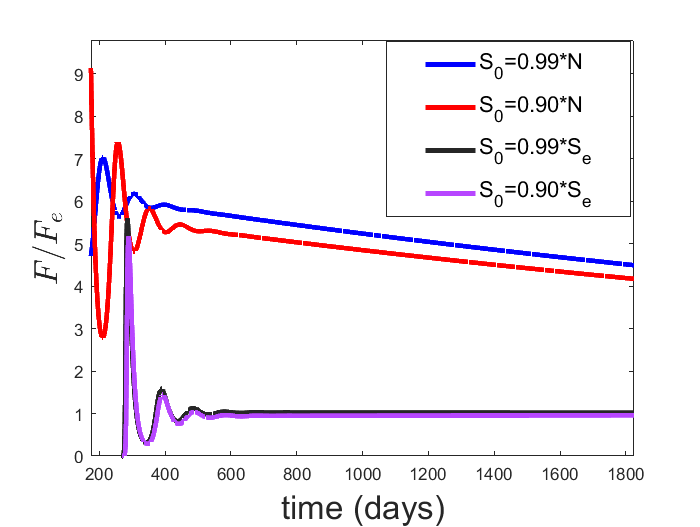
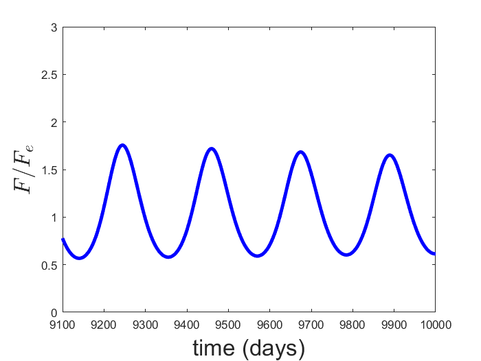
Figure 1: Time profile of the ratio $F/F_{e}$ as predicted by model (5). Left panel: case with weak Erlang memory, i.e. $K(\tau)=ae^{-a\tau}$ and exponential IFD (29). Four different initial data are reported: $S_{0}=0.90N$, $S_{0}=0.99N$, $S_{0}=0.90S_{e}$ and $S_{0}=0.99S_{e}.$ Right panel: case with strong Erlang memory kernel, i.e. $K(\tau)=a^{2}\tau e^{-a\tau}$ and IFD given by (30) (initial data $S_{0}=0.7N$). Parameter values: see the text.

Now, let us assume that the memory kernel has a strong Erlang distribution $(n=2)$ $K(\tau)=a^{2}\tau e^{-a\tau}.$ Under such hypothesis it has been shown that, when the IFD is given by (29), the endemic equilibrium of the associated SIR–M model can be destabilized via Hopf bifurcations yielding to stable recurrent oscillations [22, 24]. We recall that sufficient conditions (27) guaranteeing the local asymptotic stability of the endemic equilibrium cannot be satisfied in this case. The integral formulation of the renewal equation (5) allows to verify that the occurrence of oscillations can be observed not only when the IFD is given by (29), as already established in [22], but also in unimodal cases. As an example, consider the following IFD:

$$A_{\mu}(\tau)=\beta_{0}(\mu+\nu)^{2}\tau e^{-(\mu+\nu)\tau}.$$ (30)

We see that in this case recurrent measles waves are predicted by model (5) (see Figure 1, right panel).

6.3 SARS

In 2006, M. G. Roberts proposed an integral equation model for describing the transmission of a generic infectious disease invading a susceptible population [44]. The model was motivated by the global epidemic risk of SARS in 2003. Roberts assumed that the IF, $A(\tau),$ can be represented by the following trapezoidal distribution, requiring minimal data for its description:

$$A(\tau)=\begin{cases}p_{0}\frac{\tau-\tau_{a}}{(\tau_{b}-\tau_{a})}&\tau_{a}<\tau<\tau_{b}\\ p_{0}&\tau_{b}<\tau<\tau_{c}\\ p_{0}\frac{\tau_{d}-\tau}{(\tau_{d}-\tau_{c})}&\tau_{c}<\tau<\tau_{d}\\ 0&\text{otherwise}\end{cases}.$$ (31)

In (31), the parameter $p_{0}$ weights the contacts between the infected and susceptible individuals. It is assumed that all infected individuals have the ability to transmit the infection between time intervals $\tau_{b}$ and $\tau_{c}$ after their own infection, while no transmission occurs before time $\tau_{a}$ and after time $\tau_{d}$. The transmission probabilities between time intervals $\tau_{a}$ and $\tau_{b}$, as well as between times $\tau_{c}$ and $\tau_{d}$, are estimated through linear interpolation. Function (31) was introduced for the first time by Aldis and Roberts in order to study potential smallpox epidemics [1].

Here we employ the IF (31) into the integral model (5). We also assume that a strong Erlang distribution describes the memory of the population, $K(\tau)=a^{2}\tau e^{-a\tau}.$ Such a kernel means that the current information is un-available and the maximum weight is assigned at the information arrived to the public after a characteristic time $T=2/a$. This appears to be somehow coherent with the fact that the available information about SARS was scarce at the time it broke out.

According to [44], we take: $R_{0}=3.3$ and $(\tau_{a},\tau_{b},\tau_{c},\tau_{d})=(4,7,11,14)$ days. We also take the information parameter values $\alpha=5\cdot 10^{4}$, $a=1/30$ and the demographic parameter values $S_{0}=0.7N$, $\mu=1/75\text{ years}^{-1},$ and $N=5\cdot 10^{7}$. The parameter $p_{0}$, which can be obtained from (12), is $p_{0}=9.4\cdot 10^{-9}$.

In Figure 2, left panel, it is shown that the interplay between trapezoidal distribution (31) and the strong Erlang memory kernel produces self-sustained oscillations.

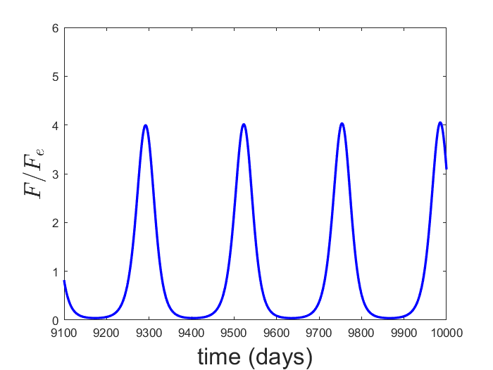
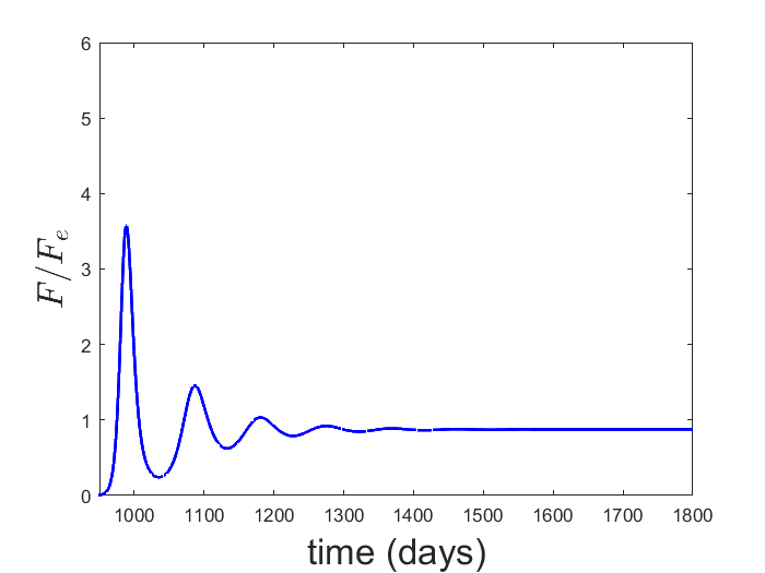
Figure 2: Time profile of the ratio $F/F_{e}$ as predicted by model (5). Left panel: case with strong Erlang memory kernel, i.e. $K(\tau)=a^{2}\tau e^{-a\tau}$ and IF given by (31). Right panel: case with weak Erlang memory kernel, i.e. $K(\tau)=ae^{-a\tau}$ and IF given by (32). The initial data is $S_{0}=0.7N$. Parameter values: see the text.

6.4 Influenza

In 2007, Roberts and coworkers [45] studied the transmission of influenza within a population by using the following IF:

$$\tilde{A}(\tau)=\frac{1}{T_{I}}A(\tau),$$ (32)

where $A(\tau)$ is given by (31) and $T_{I}$ is the mean infectious period, $T_{I}=(\tau_{d}+\tau_{c}-\tau_{a}-\tau_{b})/2$.

Here, we assume that a weak Erlang distribution describes the memory of the population, $K(\tau)=ae^{-a\tau}.$ Such a kernel means that the maximum weight is given to the current information.

According to [45], we take: $R_{0}=3$ and $(\tau_{a},\tau_{b},\tau_{c},\tau_{d})=(1.2,2.0,5.3,6.1)$ days. All the other parameter values are as in Subsection 6.3. The parameter $p_{0}$, which can be obtained from (12), is $p_{0}=6.0\cdot 10^{-8}$.

In Figure 2, right panel, it can be observed that the fraction $F/F_{e}$ slowly converges after dumped oscillations, in agreement with Theorem 5.3.

6.5 Influenza transmission within households

Glass and Becker studied the influenza transmission within households by assuming that changes in the infectiousness of individuals may be described by a deterministic birth–death process for the growth of the virus population [30]. The death rate applies once the immune system becomes active, $T_{I}$ days after infection, where $T_{I}$ is assumed to correspond to the time when symptoms first appear. The proposed infectiousness profile can be obtained, for example, by the following IF:

$$A(\tau)=\begin{cases}p_{0}e^{-2}e^{2.4\tau}&\tau\leq T_{I}\\ p_{0}e^{5}e^{-\tau}&\tau>T_{I}\end{cases},$$ (33)

We take $T_{I}=2$ and all the other parameter values are as in Subsection 6.4. The parameter $p_{0}$, which can be obtained from (12), is $p_{0}=2.2\cdot 10^{-9}$. In Figure 3, it is shown the time profile of the quantity $F(t)/F_{e}$: in the left panel we can see the epidemic waves produced by the strong Erlang memory, $K(\tau)=a^{2}\tau e^{-a\tau}$; in the right panel dumped oscillations towards a stable equilibrium may be seen in case of weak Erlang memory, $K(\tau)=ae^{-a\tau}$.

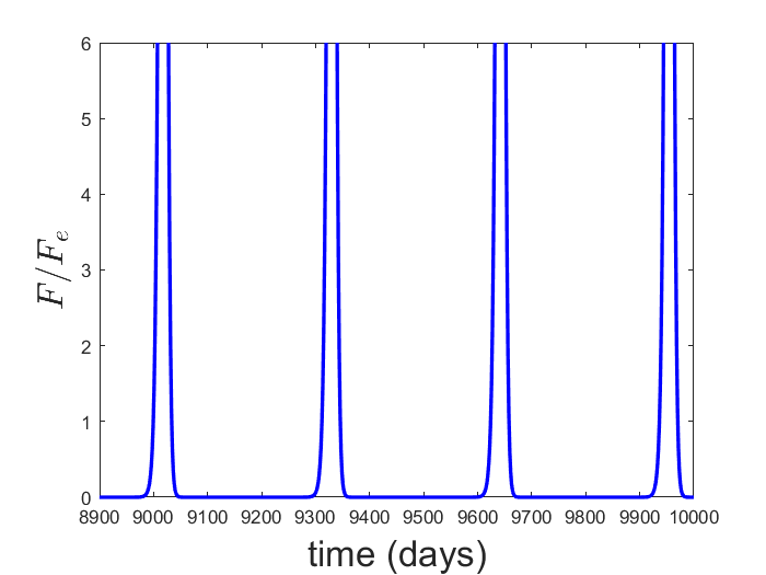
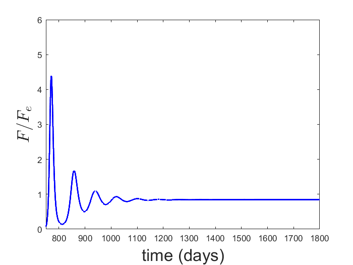
Figure 3: Time profile of the Force of infection $F$ according to model (5). Left panel: case with strong Erlang memory kernel, i. e. $K(\tau)=a^{2}\tau e^{-a\tau}$ and IF given by (33). Right panel: case with weak Erlang memory kernel, i. e. $K(\tau)=ae^{-a\tau}$ and IF given by (33). Parameter values: $R_{0}=3$, $a=1/30$, $S_{0}=0.7N$ and $N=5\cdot 10^{7}$.

7 Conclusions and future perspectives

In the field of ME, a vast portion of literature is based on the use of compartmental epidemic models that remain a natural extension of the SIR compartmental model proposed by Kermack and McKendrick. However, the early model credited to Kermack and McKendrick is well recognized as a renewal equation with an integral formulation that is more general than many compartmental models ruled by ODEs. Consequently, before building a compartmental model, it may be advisable to first attempt to formulate the problem in terms of an integral renewal equation [21]. This formulation is very significant for models incorporating the opinion-driven change of human behaviour. In fact, behavioural effects can often serve as the primary determinant in shaping the progression of an epidemic. In particular, how the population keeps memory of information and rumours regarding the disease may influence the solution of the epidemic models, thereby inducing, for example, stable recurrent oscillations which, in turn, may be interpreted as multiple epidemic waves.

In this paper, we have proposed an integral renewal equation describing the epidemic propagation of infectious diseases. The equation is behavioural in the sense that the constitutive law for the force of infection includes the information index to account for the “human element”, namely how individuals modify their risky contact according to information and rumours regarding the disease. The main results are the following:

(a) we obtain sufficient conditions, written in terms of the information parameters and functions, for the endemic equilibrium of the behavioural integral epidemic model to be locally stable. In particular, we show that the model admits a stable endemic equilibrium when the memory kernel is a weak Erlang kernel;

(b) with the aid of numerical simulations based on a non-standard numerical method, we show that the model may admit self sustained oscillations when the memory is more focused in the disease's past history, as exemplified by the strong Erlang kernel. This result is in agreement with the analysis provided by A. d'Onofrio and P. Manfredi, who proved that oscillations may be induced by information-related changes in contact patterns when the disease spread is described by a SIR model with information–dependent contact pattern [22];

(c) we also consider some different infectivity functions taken from the literature to describe infectious disease like Influenza and SARS. Still, in such cases, we show that a weak Erlang memory leads to convergence to an endemic equilibrium, while a strong Erlang memory can determine the appearance of oscillations.

Our work has, of course, a number of limitations. The qualitative analysis is limited to local stability, while global stability results are still an open problem. Another limitation is that we have considered only Erlang memory kernels, while non-Erlang distributions could be required to represent the lower time-scale of the process of formation and acquisition of information has, as compared to the memory fading of acquired information [24]. We also remark that in this paper, we extend minimal behavioural epidemic models that, while interesting as prototypes of phenomena that are not captured by the corresponding non-behavioural analogues, are unable to describe complex dynamics such as those produced, for example, by the spread of SARS-CoV-2. Future work will be devoted to the extension of more complex models: we plan to consider also the case of models, including non-mandatory pharmaceutical interventions (e.g. vaccination and treatments) whose adoption by individuals is usually strongly affected by opinion-driven change of human behaviour. Finally, the impact of host heterogeneity on epidemic dynamics has long been acknowledged [6, 20]. Recent literature introduces general Kermack and McKendrick's epidemic models that consider heterogeneity, for a population characterized by different traits, with different activity levels or disease parameters [3, 4, 8]. The provided formula expresses the FoI, delineating contributions from individuals infected at a specific time and with a particular trait. This suggests, as a natural extension, a generalization of the constitutive law for the FoI with an information index aimed at exploring how heterogeneity influences epidemic aspects in a model that incorporates human behaviour and broadens the analysis presented in this paper.

Acknowledgements

This work has been performed under the auspices of the Italian National Group for Scientific Computing (GNCS) and the Italian National Group for Mathematical Physics (GNFM) of the National Institute for Advanced Mathematics (INdAM).
B.B. acknowledges EU funding within the NextGenerationEU—MUR PNRR Extended Partnership initiative on Emerging Infectious Diseases (Project no. PE00000007, INF-ACT).
B.B. also acknowledges PRIN 2020 project (No. 2020JLWP23) ``Integrated Mathematical Approaches to Socio–Epidemiological Dynamics''.

Appendix A Discretization scheme

Consider an uniform mesh $t_{n}=nh$, where $n=0,1,\dots$, and $h>0$ is the stepsize. We define the following discretization scheme for the continuous model (5):

$$S_{n+1} =S_{n}+h\big{(}\lambda-\mu S_{n+1}-\beta(M_{n})S_{n+1}F_{n}\big{)},$$

$$F_{n+1} =F_{0}(t_{n+1})+h\sum_{j=0}^{n}A_{\mu}(t_{n+1-j})\beta(M_{j})F_{j}S_{j+1},$$ (34)

$$M_{n+1} =M_{0}(t_{n+1})+h\sum_{j=0}^{n}K(t_{n+1-j})g(F_{j}),$$

for $n=0,1,\dots$, where the forcing functions $F_{0}(t)$ and $M_{0}(t)$ are given by (28) and $\eqref{forcingFM}_{2}$, respectively. Here, $S_{n}\approx S(t_{n})$, $F_{n}\approx F(t_{n})$, $M_{n}\approx M(t_{n})$ for $n=0,1,\dots$ and $S_{0}=S(0)$, $F_{0}=F_{0}(0)$ and $M_{0}=M_{0}(0)$. This numerical method is called non-standard because it is based on a modified rectangular rule, which is implicit in $S$ and explicit in $F$ and $M$. A detailed analysis of the qualitative and asymptotic behaviour of the numerical solution to (5), obtained by (A), is presented in [14]. Here we enunciate the main results.

Denote by

$$\textbf{{e}}(h;t_{n})=\begin{bmatrix}S(t_{n})\\ F(t_{n})\\ M(t_{n})\end{bmatrix}-\begin{bmatrix}S_{n}\\ F_{n}\\ M_{n}\end{bmatrix},$$

the global error of discretization (A).

Theorem A.1.

Assume that the infectivity function $A(\tau)$ is continuously differentiable on an interval $[0,T]$ and that $\{S_{n}\}_{n\in\mathbb{N}_{0}}$, $\{F_{n}\}_{n\in\mathbb{N}_{0}}$ and $\{M_{n}\}_{n\in\mathbb{N}_{0}}$ are the approximations to the solution of (5), defined by (A). Let $h=T/\bar{n}$, where $\bar{n}$ is a positive integer, then

$$\lim_{h\rightarrow 0}\max_{0\leq n\leq\bar{n}}||\textbf{e}(h;t_{n})||=0.$$

Furthermore, the convergence rate is linear.

Theorem A.2.

Consider equation (A), the following inequalities hold: $0<S_{n}\leq S_{\max}(h),$ $0\leq F_{n}\leq F_{\max}(h)$ and $0\leq M_{n}\leq M_{\max}(h)$, for $n=0,1,\dots$ and $h>0$. Here $S_{\max}(h),F_{\max}(h)$ and $M_{\max}(h)$ are positive constants.

The definition of the numerical basic reproduction number

$$R_{0}(h)=\frac{\lambda}{\mu}\bar{A}_{\mu}(1,h),$$

with $\bar{A}_{\mu}(1,h)=h\sum_{j=1}^{\infty}A_{\mu}(t_{j})$, as the discrete equivalent to (12), allows an investigation about the equilibria of the discrete system (A), which parallels the one reported in Sections 4-5. In particular, if $R_{0}(h)>1$, then system (A) admits a unique endemic equilibrium that we denote by $EE(h)=(S_{e}(h),F_{e}(h),M_{e}(h))$. The endemic equilibria are obtained from the following conditions:

$$M_{e}(h)=\bar{K}(1,h)g(F_{e}(h)),\quad\quad S_{e}(h)=\frac{\lambda}{\mu R_{0}(h)\beta(\bar{K}(1,h)g(F_{e}(h))},$$

and $F_{e}(h)$ is the solution of the non linear equation

$$x-\mu R_{0}(h)+\frac{\mu}{\beta(\bar{K}(1,h)g(x))}=0,$$

in the interval $[0,F_{max}(h)]$, where $\bar{K}(1,h)=h\sum_{j=1}^{\infty}K(t_{j})$. Set $\bar{A}_{\mu}(z,h)=h\sum_{j=1}^{\infty}A_{\mu}(t_{j})z^{j}$ and $\bar{K}(z,h)=h\sum_{j=1}^{\infty}K(t_{j})z^{j}$, the following theorem gives a sufficient condition for the local asymptotic stability of the equilibria.

Theorem A.3.

Let be $h>0$. Any equilibrium $EE(h)$ of model (A) is locally asymptotically stable if the characteristic equation

$$\beta(M_{e}(h))S_{e}(h)\bar{A}_{\mu}(z,h)\bigg{(}1+\frac{g^{\prime}(F_{e}(h))\beta^{\prime}(M_{e}(h))F_{e}(h)\bar{K}(z,h)}{\beta(M_{e}(h))}\bigg{)}=1+h\frac{\beta(M_{e}(h))F_{e}(h)}{1-z+\mu h},$$

has no solution for $|z|\leq 1$.

From Theorem A.3 sufficient conditions, written in terms of the information parameters and functions, for the numerical endemic equilibrium to be locally stable, are derived. The reader is referred to [13]. A comparison with the results of Section 5 confirms that the numerical solution replicates the stability properties of the continuous one. Furthermore, as $h\rightarrow 0$ the accuracy with which the numerical method approximates the entire dynamics of the continuous system (5) increases.

Appendix B Paley-Wiener Theorem

The theory on the asymptotic stability of Volterra integral equations of convolution type is essentially based on the Paley-Wiener theorem [43, p. 59]. An extension of this result to the case where the matrix kernel does not belong to $L^{1}(0,\infty)$ is provided by Ch. Lubich [36, Th. 9.1]. Here, we report this result for the sake of completeness.

Theorem B.1.

Consider the system of Volterra integral equations

$$\textbf{y}(t)=\textbf{f}(t)+\int_{0}^{t}\mathcal{\textbf{Q}}(t-\tau)\textbf{y}(\tau)ds,$$ (35)

where the matrix $\mathcal{\textbf{Q}}(\cdot)$ and the function $\textbf{f}(t)$ satisfy

$$\mathcal{\textbf{Q}}(\cdot)=\textbf{B}(\cdot)+\textbf{A}_{\infty},\quad\textbf{A}_{\infty}=\underbrace{\begin{bmatrix}\textbf{A}^{1}_{\infty}\\ 0\end{bmatrix}}_{d}\begin{array}[]{l}\}l\\ \}k\end{array},\quad\textbf{f}(t)=\begin{bmatrix}\textbf{f}_{0}(t)\\ \textbf{f}_{1}(t)\end{bmatrix}\begin{array}[]{l}\}l\\ \}k\end{array},$$ (36)

with $\textbf{B}(\cdot)\in L^{1}(0,\infty)$ and $k=d-l=$dimension of the null space of $\textbf{A}_{\infty}$. Then $\textbf{y}(t)\rightarrow 0$, whenever $\textbf{f}^{\prime}_{0}(t),$ $\textbf{f}_{1}(t)\longrightarrow 0$ for $t\rightarrow\infty$, if and only if the equation

$$w^{l}\text{det}\Big{(}I-\int_{0}^{\infty}\mathcal{\textbf{Q}}(t)e^{-wt}dt\Big{)}=0,$$ (37)

has no solution for $Re(w)\geq 0$.

Remark B.1.

For $Re(w)=0$, equation (37) must be interpreted as limit for $\tilde{w}\rightarrow w$, $Re(\tilde{w})>0$.

References

- [1] G. K. Aldis and M. G. Roberts. An integral equation model for the control of a smallpox outbreak. Mathematical Biosciences, 195(1):1–22, 2005.
- [2] Z. Bai. Global dynamics of a SEIR model with information dependent vaccination and periodically varying transmission rate. Mathematical Methods in the Applied Sciences, 38(11):2403–2410, 2014.
- [3] M. C. J. Bootsma, K. M. D. Chan, O. Diekmann, and H. Inaba. The effect of host population heterogeneity on epidemic outbreaks. arXiv preprint arXiv:2308.06593, 2023.
- [4] M. C. J. Bootsma, K. M. D. Chan, O. Diekmann, and H. Inaba. Separable mixing: the general formulation and a particular example focusing on mask efficiency. Mathematical Biosciences and Engineering, 20(10):17661–17671, 2023.
- [5] F. Brauer. Age of infection in epidemiology models. Electronic Journal Differential Equations, 12:29–37, 2005.
- [6] F. Brauer. Epidemic models with heterogeneous mixing and treatment. Bulletin of Mathematical Biology, 70(7):1869–1885, 2008.
- [7] F. Brauer, C. Castillo-Chavez, and Z. Feng. Mathematical Models in Epidemiology, volume 69 of Texts in Applied Mathematics. Springer, New York, 2019.
- [8] F. Brauer and J. Watmough. Age of infection epidemic models with heterogeneous mixing. Journal of Biological Dynamics, 3(2-3):324–330, 2009.
- [9] D. Breda, O. Diekmann, W. F. de Graaf, A. Pugliese, and R. Vermiglio. On the formulation of epidemic models (an appraisal of Kermack and McKendrick). Journal of Biological Dynamics, 6:103–117, 2012.
- [10] B. Buonomo and R. Della Marca. Effects of information-induced behavioural changes during the COVID-19 lockdowns: the case of Italy. Royal Society Open Science, 7(10):201635, 2020.
- [11] B. Buonomo and R. Della Marca. A behavioural vaccination model with application to meningitis spread in Nigeria. Applied Mathematical Modelling, 125:334–350, 2024.
- [12] B. Buonomo, R. Della Marca, A. d’Onofrio, and M. Groppi. A behavioural modelling approach to assess the impact of COVID-19 vaccine hesitancy. Journal of Theoretical Biology, 534:110973, 2022.
- [13] B. Buonomo, E. Messina, C. Panico, and A. Vecchio. An integral renewal equation approach to behavioural epidemic models with information index. In prep.
- [14] B. Buonomo, E. Messina, C. Panico, and A. Vecchio. A stable numerical method for integral epidemic models with behavioural changes in contact patterns. In preparation.
- [15] V. Capasso. Mathematical Structures of Epidemic Systems, volume 97 of Lecture Notes in Biomathematics. Springer-Verlag, Berlin, 1993.
- [16] V. Capasso and G. Serio. A generalization of the Kermack-McKendrick deterministic epidemic model. Mathematical Biosciences, 42(1–2):43–61, 1978.
- [17] F. Della Rossa, D. Salzano, A. Di Meglio, F. De Lellis, M. Coraggio, C. Calabrese, A. Guarino, R. Cardona-Rivera, P. De Lellis, D. Liuzza, F. Lo Iudice, G. Russo, and M. di Bernardo. A network model of Italy shows that intermittent regional strategies can alleviate the COVID-19 epidemic. Nature communications, 11(1):5106, 2020.
- [18] O. Diekmann, M. Gyllenberg, and J. A. J. Metz. Finite dimensional state representation of linear and nonlinear delay systems. Journal of Dynamics and Differential Equations, 30(4):1439–1467, 2018.
- [19] O. Diekmann and J. A. P. Heesterbeek. Mathematical Epidemiology of Infectious Diseases: Model Building, Analysis and Interpretation. Wiley Series in Mathematical and Computational Biology. John Wiley & Sons, Ltd., Chichester, 2000.
- [20] O. Diekmann, J. A. P. Heesterbeek, and J. A. J. Metz. On the definition and the computation of the basic reproduction ratio in models for infectious diseases in heterogeneous populations. Journal of Mathematical Biology, 28:365–382, 1990.
- [21] O. Diekmann and H. Inaba. A systematic procedure for incorporating separable static heterogeneity into compartmental epidemic models. Journal of Mathematical Biology, 86(2):29, 2023.
- [22] A. d'Onofrio and P. Manfredi. Information–related changes in contact patterns may trigger oscillations in the endemic prevalence of infectious diseases. Journal of Theoretical Biology, 256(3):473–478, 2009.
- [23] A. d'Onofrio and P. Manfredi. The interplay between voluntary vaccination and reduction of risky behavior: a general behavior-implicit SIR model for vaccine preventable infections. Current Trends in Dynamical Systems in Biology and Natural Sciences. SEMA SIMAI Springer Series, 21:185–203, 2020.
- [24] A. d'Onofrio and P. Manfredi. Behavioral SIR models with incidence-based social-distancing. Chaos, Solitons and Fractals, 159:112072, 2022.
- [25] A. d'Onofrio, P. Manfredi, and E. Salinelli. Vaccinating behaviour, information, and the dynamics of SIR vaccine preventable diseases. Theoretical Population Biology, 71(3):301–317, 2007.
- [26] A. d’Onofrio, M. Iannelli, P. Manfredi, and G. Marinoschi. Optimal epidemic control by social distancing and vaccination of an infection structured by time since infection: The COVID-19 case study. SIAM Journal on Applied Mathematics, S199–S224, 2023.
- [27] N. M. Ferguson, D. Laydon, G. Nedjati-Gilani, N. Imai, K. Ainslie, M. Baguelin, S. Bhatia, A. Boonyasiri, Z. Cucunubá, G. Cuomo-Dannenburg, et al. Report 9: Impact of non-pharmaceutical interventions (NPIs) to reduce COVID-19 mortality and healthcare demand. Technical Report 10.25561, Imperial College London, 2020.
- [28] E. Fesce, G. Marini, R. Rosà, D. Lelli, M. P. Cerioli, M. Chiari, M. Farioli, and N. Ferrari. Understanding West Nile virus transmission: Mathematical modelling to quantify the most critical parameters to predict infection dynamics. PLOS Neglected Tropical Diseases, 17(5):e0010252, 2023.
- [29] M. Gatto, E. Bertuzzo, L. Mari, S. Miccoli, L. Carraro, R. Casagrandi, and A. Rinaldo. Spread and dynamics of the COVID-19 epidemic in Italy: Effects of emergency containment measures. Proceedings of the National Academy of Sciences, 117(19):10484–10491, 2020.
- [30] K. Glass and N. G. Becker. Estimating antiviral effectiveness against pandemic influenza using household data. Journal of the Royal Society Interface, 6(37):695–703, 2009.
- [31] W. O. Kermack and A. G. McKendrick. A contribution to the mathematical theory of epidemics. Proceedings of the Royal Society of London. Series A, 115(772):700–721, 1927.
- [32] W. O. Kermack and A. G. McKendrick. Contributions to the mathematical theory of epidemics–I. Bulletin of Mathematical Biology, 53(1):33–55, 1991.
- [33] A. Kumar, P. K. Srivastava, and R. Gupta. Nonlinear dynamics of infectious diseases via information-induced vaccination and saturated treatment. Mathematics and Computers in Simulation, 157:77–99, 2019.
- [34] D. Lacitignola and G. Saccomandi. Managing awareness can avoid hysteresis in disease spread: an application to coronavirus COVID-19. Chaos, Solitons and Fractals, 144:110739, 2021.
- [35] R. López-Cruz. Global stability of an SAIRD epidemiological model with negative feedback. Advances in Continuous and Discrete Models, 2022(1):41, 2022.
- [36] C. Lubich. On the stability of linear multistep methods for Volterra convolution equations. IMA Journal of Numerical Analysis, 3(4):439–465, 1983.
- [37] P. Manfredi and A. d'Onofrio, editors. Modeling the Interplay between Human Behavior and the Spread of Infectious Diseases. Springer, New York, 2013.
- [38] M. Martcheva. An Introduction to Mathematical Epidemiology, volume 61 of Texts in Applied Mathematics. Springer, New York, 2015.
- [39] E. Messina, M. Pezzella, and A. Vecchio. A non-standard numerical scheme for an age-of-infection epidemic model. Journal of Computational Dynamics, 9(2):239–252, 2022.
- [40] E. Messina, M. Pezzella, and A. Vecchio. Nonlocal finite difference discretization of a class of renewal equation models for epidemics. Mathematical Biosciences and Engineering, 20(7):11656–11675, 2023.
- [41] R. K. Miller. On the linearization of Volterra integral equations. Journal of Mathematical Analysis and Applications, 23(1):198–208, 1968.
- [42] C. E. Overton, L. Pellis, H. B. Stage, F. Scarabel, J. Burton, C. Fraser, I. Hall, T. A. House, C. Jewell, A. Nurtay, F. Pagani, and K. A. Lythgoe. EpiBeds: Data informed modelling of the COVID-19 hospital burden in England. PLOS Computational Biology, 18(9):e1010406, 2022.
- [43] R. E. A. C. Paley and N. Wiener. Fourier Transforms in the Complex Domain. American Mathematical Society, 1934.
- [44] M. G. Roberts. Modeling strategies for containing an invading infection. Mathematical Population Studies, 13(4):205–214, 2006.
- [45] M. G. Roberts, M. Baker, L. C. Jennings, G. Sertsou, and N. Wilson. A model for the spread and control of pandemic influenza in an isolated geographical region. Journal of the Royal Society Interface, 4(13):325–330, 2007.
- [46] J. Rui, Q. Wang, J. Lv, B. Zhao, Q. Hu, H. Du, W. Gong, Z. Zhao, J. Xu, Y. Zhu, et al. The transmission dynamics of Middle East Respiratory Syndrome coronavirus. Travel Medicine and Infectious Disease, 45:102243, 2022.
- [47] S. Saha, G. P. Samanta, and J. J. Nieto. Epidemic model of COVID-19 outbreak by inducing behavioural response in population. Nonlinear Dynamics, 102:455–487, 2020.
- [48] P. van den Driessche and J. Watmough. A simple SIS epidemic model with a backward bifurcation. Journal of Mathematical Biology, 40(6):525–540, 2000.
- [49] W. Wang. Epidemic models with nonlinear infection forces. Mathematical Biosciences and Engineering, 3(1):267, 2006.
- [50] Z. Wang, C. T. Bauch, S. Bhattacharyya, A. d'Onofrio, P. Manfredi, M. Perc, N. Perra, M. Salathé, and D. Zhao. Statistical physics of vaccination. Physics Reports, 664:1–113, 2016.
- [51] J. Yang, M. Martcheva, and Y. Chen. Imitation dynamics of vaccine decision-making behaviours based on the game theory. Journal of Biological Dynamics, 10(1):31–58, 2016.
- [52] C. Zuo, Y. Ling, F. Zhu, X. Ma, and G. Xiang. Exploring epidemic voluntary vaccinating behavior based on information-driven decisions and benefit-cost analysis. Applied Mathematics and Computation, 447:127905, 2023.