Demystifying Quantum Power Flow:
Unveiling the Limits of Practical Quantum Advantage

Abstract

Quantum computers hold promise for solving problems intractable for classical computers, especially those with high time and/or space complexity. The reduction of the power flow (PF) problem into a linear system of equations, allows formulation of quantum power flow algorithms, based on quantum linear system solving methods such as the Harrow-Hassidim-Lloyd (HHL) algorithm. The speedup due to QPF algorithms is often claimed to be exponential when compared to classical PF solved by state-of-the-art algorithms. We investigate the potential for practical quantum advantage in solving QPF compared to classical methods on gate-based quantum computers. We meticulously scrutinize the end-to-end complexity of QPF approach, providing a nuanced evaluation of the purported quantum speedup in this problem. Our analysis establishes a best-case bound for the HHL-based quantum power flow complexity, conclusively demonstrating that HHL-based method has higher runtime complexity compared to classical algorithm for solving the direct current power flow (DCPF) and fast decoupled load flow problem. Additionally, we establish that for potential PQA to exist it is necessary to consider DCPF-type problems with a very narrow range of condition number values and readout requirements.

I Introduction

The simultaneous task of providing electrical energy to the world and fighting climate change by switching transportation to electricity will require electricity generation to increase by more than two and half times by 2050, from 2021 levels [1]. This increased reliance on electricity will make secure power grid operation an even more important challenge. Modern power system operation heavily relies on the ability of system operators to compute the system state accurately and efficiently. The fundamental computational tool underpinning this analysis is the power flow problem, which is solved to obtain node voltages and line flows for a given set of nodal power injections [2]. Direct current power flow (DCPF) approximation is a popular approach as it provides a fast, unique, and reliable solution to the power flow problem [3, 4, 5, 6, 7, 8]. From a computational standpoint, the DCPF problem translates to solving a linear system of equations given a nodal power injection vector. This implies that with an increase in system size and changes in the injection vector due to uncertainty, the computational effort required to conduct a DCPF analysis increases. In addition to DCPF, another prominent linear power flow formulation called fast decoupled load flow (FDLF) also reduces to solving a sequence of linear systems of equations [2]. In practice, algorithms such as the conjugate gradient (CG) method are used to solve these linear power flow problems for large-scale systems, exploiting features such as sparsity for faster convergence to the solution [9].

Quantum computing (QC), in theory, can provide provably asymptotic speedups over classical computers for many problems of practical interest [10, 11, 12]. QC achieves this by exploiting inherently quantum properties such as superposition and entanglement. This leads to novel algorithmic techniques in QC that cannot be emulated efficiently by classical computers. One such algorithmic primitive developed in QC literature is an exponentially fast linear system solver, first introduced in the work of Harrow, Hassidim, and Lloyd (HHL) [13] and improved upon by others [14, 15]. The exponential speed up in these works comes from the fact that linear system solving subroutine can solve a sparse linear system in time that scales only logarithmically with system size, if the input to the subroutine is provided as a quantum state and if relevant output information can be extracted using a small number of quantum measurements. The input/output model used in these algorithms is markedly different from those in classical computing. This indicates that a true end-to-end exponential speed-up cannot be claimed over classical algorithms in general. This point has been noted before in QC literature [16] and in some cases the claimed exponential speedup has been shown to vanish when the classical computer is given access to a data input/output model that appropriately matches the data model used by the QC algorithm [17, 18, 19].

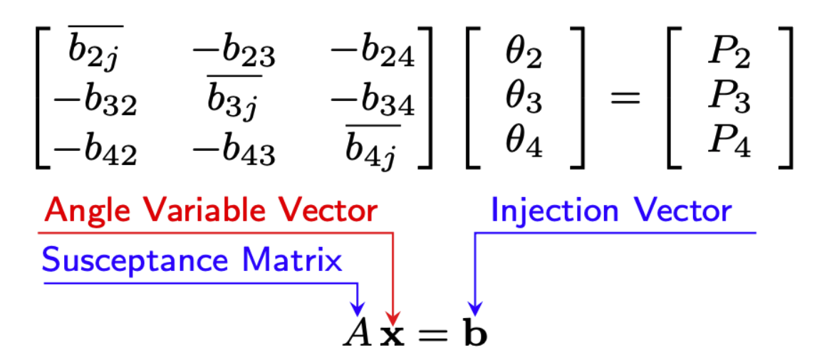
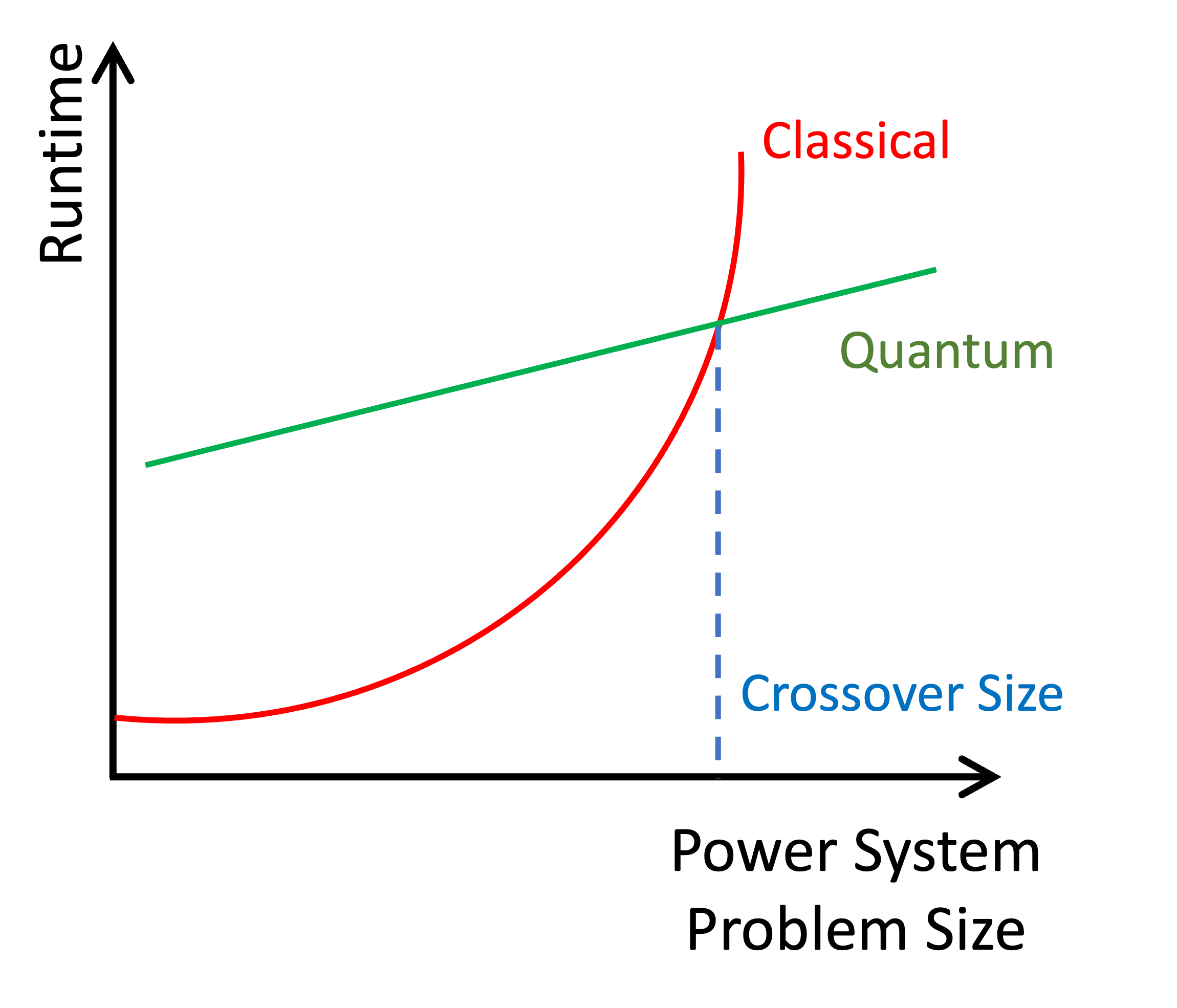
Figure 1: Power network data, equivalent linear system of equations, and the idea of practical quantum advantage (PQA). Left: Consider a simplified power grid with four “buses” (nodes) connected by five “branches” (lines). Each line has a certain “susceptance” which affects how easily electricity flows through it. Using direct current approximations [3], we can approximate the network by focusing only on these susceptances and ignoring other electrical properties (In the DC power flow approximation, the network is assumed to be lossless, the phase-angle differences between nodes are considered small, and all node voltages are assumed to be approximately equal to one per unit [3]). The unknowns in this system are the bus angle values (depicted in red) which depend on known quantities like susceptance (depicted in blue). Without any loss of generality, we can set one of the bus angle values to zero. Center: To solve the problem, DCPF converts the grid into a set of equations. It uses the susceptance values, known bus angles, and power injections (how much electricity enters or leaves each bus) to calculate the unknown bus angle values. It can be shown that the $A$ in this system is always positive by diagonal dominance arguments[3]. Right: Complexity analysis of classical and quantum approaches to this problem tells us how their respective runtimes scale with problem size and other parameters. PQA can exist only if there is a crossover point as depicted in this figure. Such a crossover implies that there exists a system size beyond which quantum algorithms can be faster for solving this problem.

Classical Input $$\xRightarrow{\scalebox{0.9}{~{}~{} {{\color[rgb]{1,0,0}Classical Algorithm}}}~{}~{}}{\color[rgb]{0.3,0,0}\textsc{{Classical Output}}}$$

$${\color[rgb]{0.3,0,0}\textsc{{Classical Input}}}\xRightarrow{\scalebox{0.8}{{~{}~{} {\color[rgb]{1,0,0}State Prep.}}}~{}~{}}{\color[rgb]{0,0,1}\Big{|}\textsc{{Input}}\Big{\rangle}} \xRightarrow{\scalebox{0.9}{{~{}~{} {\color[rgb]{1,0,0}Quantum Algorithm}}}~{}~{}}{\color[rgb]{0,0,1}\Big{|}\textsc{{Output}}\Big{\rangle}}\xRightarrow{\scalebox{0.8}{{~{}~{} {\color[rgb]{1,0,0}Readout}}}~{}~{}}{\color[rgb]{0.3,0,0}\textsc{{Classical Output}}}$$

Figure 2: A simple information flow schematic of solving any problem using classical and quantum algorithms. From Figure 1, classical input is $\mathbf{b}$, and classical output is $\mathbf{x}$. The quantum algorithm encodes the matrix $A$ (considering $A$ as a Hamiltonian for a quantum system) in terms of time evolution operator $e^{iAt}$. As depicted here, solving a linear system using quantum computing via the HHL algorithm involves three steps [20]: i) state preparation; ii) state propagation (quantum algorithm), and iii) readout. In the state preparation step problem parameter $\mathbf{b}$ is encoded into a quantum state $|\Psi_{o}\rangle$. Following this, the second step is the application of quantum gates (unitary operations) to evolve the initial quantum state $|\Psi_{o}\rangle$ into final state $|\tilde{\textbf{x}}\rangle$ based on the properties of the matrix $A$. Here, $|\tilde{\textbf{x}}\rangle$ is a quantum state and the third step is readout, where $|\tilde{\textbf{x}}\rangle$ is measured to extract the solution to the linear system $\widehat{\mathbf{x}}$. We assess the quantum advantage based on the end-to-end run-time complexities for the DCPF problem. Here, end-to-end complexity in QC refers to the comprehensive time complexity from input to output, encompassing all stages of solving the DCPF problem, and not just the cost of running a quantum circuit that is a subroutine of the full solution method The end-to-end complexity determines the existence of PQA for these problems as it tells us how the total runtime required to solve this problem scales with the size of the system and other parameters in realistic DCPF problems.

In recent times, QC has garnered significant attention in the power systems community, with efforts directed towards solving power flow problems through QC techniques, referred to as quantum power flow (QPF) [21, 22, 23, 24, 25, 26, 27, 28, 29, 30, 31]. The primary rationale behind these endeavors lies in QC’s theoretical ability to efficiently solve a linear systems of equations. This is particularly pertinent as various power flow formulations, such as DCPF and FDLF, are either equivalent or can be reduced to solving linear systems of equations [3, 2]. In [21, 23, 22], the authors suggest employing the HHL algorithm to solve FDLF on a quantum computer, implying a potential exponential speed-up due to the runtime complexity of HHL. Authors in [23] present results obtained using a real quantum computer for solving the FDLF problem. The authors in [21] and [22] propose exponential speedup but the complexities associated with the readout of FDLF iteration outputs have not been addressed. This aspect, as highlighted in [23], is crucial for the execution of FDLF. Additionally, in [23], the authors rightly argue that quantum memory is indispensable for attaining quantum speedup in FDLF and suggest probabilistic Monte-Carlo simulation-type problems as potential applications of QPF. However, the paper does not analyze end-to-end complexity including the stages like state preparation. To alleviate qubit requirements, [28] proposes a hybrid method. Additionally, [30, 24] describes variational QPF to reduce the circuit depth needed to solve QPF compared to HHL-based QPF [21]. Authors in [24] provide a comprehensive review of different QPF formulations and highlight the need to multiply the ‘downloading and uploading’ complexities in HHL-QPF complexity, however, their effect on quantum speedup remains to be explored.

Due to these limitations of existing discussions on QPF formulations there is a lack of a thorough assessment of the requirements for a practical quantum advantage (PQA). Quantum advantage refers to the potential computational superiority of quantum computers over classical computers for specific problems [32]. The challenge in the PQA assessment can be linked to plotting a runtime complexity or resource requirement curve, as illustrated in the rightmost subplot of Figure 1. In the context of DCPF, identifying the crossover point on this plot, that is, where the quantum computer’s resource requirements become more favorable than the best-known classical method, holds significant implications for the practical adoption of QC in power systems. If such a crossover point does not exist or if the crossover point exceeds the size of real-world problems (e.g., a billion-node power flow problem), the adoption of QC may not be practically justified. Specifically for the QPF problem, achieving PQA involves demonstrating that a quantum algorithm can efficiently provide the complete network state vector (including both the voltage angle and magnitude, depending on the formulation) by solving a power flow problem, significantly faster or with fewer computational resources and with the desired level of accuracy, than the best-known classical algorithms.

In this paper, we elaborate on the complexities associated with each step of solving the QPF, shown in Figure 2. Further, the exponential speed-up claim of HHL-QPF methods is critically weighted against various HHL caveats [16]. Further, by doing the end-to-end complexity assessment for this problem we attempt to build a framework to assess:

• Does practical quantum advantage exist in ‘solving’ the DCPF problem?

  • If yes, at what power system size will the runtime complexity of quantum computing methods surpass that of classical methods?

  • If no, what essential features must a DCPF-type problem have to show potential for PQA?

This work does not solve QPF, but instead hones the runtime complexity of QPF by considering the end-to-end time requirements and incorporating the key parameters from realistic AC power network datasets [35]. The main contributions of this paper can be summarized as:

• Demonstration that the end-to-end runtime complexity of solving the DCPF problem through the HHL-QPF algorithm is asymptotically worse than that of the classical CG method. When considering the read-out [34] requirement in QC and condition number growth with network size ($N$ Buses) for realistic AC power network datasets [35], the complexity of HHL-QPF becomes $\mathcal{O}(N^{4.62}\log N)$, whereas the CG method’s complexity for solving an $N$-Bus DCPF problem remains $\mathcal{O}(N^{1.90}\log N)$. The effect of runtime overhead of state preparation is also discussed.

• Identifying the power network parameter range (condition number) and readout level for the types of the power flow-type problems for which practical quantum advantage can potentially exist. We show that for readout requirement of $D$ states and condition number $\kappa$, problem parameters must satisfy $D\kappa^{3/2}\ll Ns^{-1}$ to have any potential PQA using the HHL algorithm.

II DC Power Flow Problem

The DCPF equations can be obtained by applying several simplifying assumptions to the non-linear alternating current (AC) branch flow equations [3]. These assumptions lead to conditions where the power balance equations can be expressed as a weighted sum of angle differences between buses. The weights in this sum are represented by the elements of the susceptance matrix as shown in Figure 1. In matrix form the DCPF is,

$$A\mathbf{x}=\mathbf{b}$$ (1)

with $A$ being positive definite, symmetric matrix of size $N\times N$ where $N$ is one less than system size, $\mathbf{x}$ and $\mathbf{b}$ are $N$-dimensional vectors.

The runtime complexity to solve (1) using Gaussian elimination is $\mathcal{O}(N^{3})$ or precisely $\mathcal{O}(N^{\omega})$ where $\omega\in[2,2.372)$ denotes the matrix multiplication exponent [12]. This complexity becomes prohibitive in solving DCPF for large-scale systems because an industry scale network of 10,000 buses will require $\sim 10^{10}$ operations, which is daunting for classical computers processing operations at gigahertz speeds. Further, exact methods are not always able to exploit the sparsity present in system matrix $A$. In a power network, each node is connected to only a few other nodes of the network grid. Thus, sparsity is present in $A$ for all practical power networks. Figure 3 (left) shows the sparsity level for different systems from PGLib[35] library, which includes over sixty open-access transmission network datasets.

Further, a computational gain can come from the fact that we do not require the exact solution of $\mathbf{x}$ in DCPF problem. This is because the least count of the measurement devices in a power network is much higher than computing machine precision, and thus an error of the order $10^{-6}$ is generally sufficient.

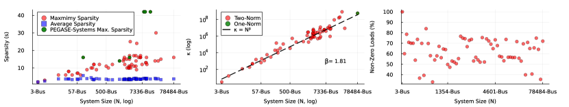
Figure 3: Network properties of the PGLib [35] power transmission network datasets reveal structural insights and potential numerical challenges in solving DCPF. Left: Level of sparsity ($s$) for different power system size ($N$-Buses). Here, average sparsity is the average number of non-zero elements in any row of matrix $A$. The PEGASE grids tend to have higher $s$ values due to sub-system equivalencies. Sparsity levels are below 30 for most of the 66 power grids from PGLib, with an average sparsity under 10, highlighting the potential for efficient sparse matrix techniques. Center: Polynomial relationship of condition number ($\kappa$) of $A$ with power system size ($N$ Buses). The one-norm is used to lower bound $\kappa$ for the 78484-Bus system due to computational restrictions of calculating the two-norm of such a large system. Condition number exhibits a polynomial (near-quadratic) growth trend with increasing system size ($N$-Buses), signaling potential numerical challenges and runtime increase in solving DCPF. Right: Percentage of non-zero elements in load vectors (sparsity percentage) for different PGLib systems. It shows that load vector sparsity will not be able to reduce the encoding complexity of $\mathbf{b}$ vector beyond a certain level. More importantly, due to the nature of power grid operation applications, one cannot make strong assumptions about or requirements on load-vector sparsity levels.

III Classical Method Complexity

The Conjugate Gradient (CG) method is among the best algorithms in terms of asymptotic complexity for solving linear systems of equations with a sparse, positive definite matrix $A$. As the power system matrices fulfill both conditions, we focus on analyze CG as one of the best ways to solve DCPF classically. We define $s$ as the maximum number of non-zero values in a row i.e. sparsity, and $\kappa$ as condition number ($\kappa=\|A^{-1}\|\|A\|$). The total complexity of CG can be split into two parts: complexity of dominant operations and number of times dominant operations are used.

Now, considering the dominant operation complexity of matrix-vector multiplication, $\mathcal{O}(Ns),$ and upper bound on number of iterations required to achieve the error $\varepsilon_{c}$ (details are given in supplementary information), the overall complexity of the CG for solving (1) is $\mathcal{O}(N\sqrt{\kappa}s\log({1}/{\varepsilon_{c}}))$. Further, read-write complexity for the sparse matrix $A$ is $\mathcal{O}(Ns)$ (higher than $\mathbf{b},\mathbf{x}$ read-out costs which is $\mathcal{O}(N)$) and this additional cost is additive to the runtime complexity. Here, additive means that we read $A,\mathbf{b}$ once before solving (1) and read $\mathbf{x}\in\mathbb{R}^{N}$ once after solving the problem. To obtain $\mathbf{x}$ one does not need to repeat CG but only needs to read it with complexity $\mathcal{O}(N)$. This is important as additive terms are subsumed into dominant complexity terms and do not alter the end-to-end complexity. Thus, the end-to-end complexity of solving DCPF (1) using CG is $\mathcal{O}(Ns+N\sqrt{\kappa}s\log({1}/{\varepsilon_{c}})+N)=\mathcal{O}(N\sqrt{\kappa}s\log({1}/{\varepsilon_{c}}))$. Further, along with exploiting sparsity, CG runtime complexity has square root dependence condition number $\kappa$, making it highly efficient for DCPF as $\kappa$ has polynomial growth from Figure 3 (center).

From the definition of $\varepsilon_{c}$ and error vectors ($\mathbf{e}^{o}$ and $\mathbf{e}^{i}$, details are given in supplementary material), it is clear that CG error upon convergence will depend on initial point $\mathbf{x}_{o}$. It is clear that if a starting point is closer to the final solution, the same value of $\varepsilon_{c}$ can be achieved in fewer CG iterations. This feature of CG has led to considerable efforts on finding ‘good’ starting points of phase-angles ($\mathbf{x}$) in DCPF problems, particularly when DCPF needs to be solved repeatedly with small perturbations in the power injections ($\mathbf{b}$), known as hot-starting of DCPF [3]. Also, the error is expressed in terms of the energy norm, $\|e^{i}\|_{A}$ (see supplementary information for more details on error definitions.). Therefore, the effects of the definition of $\varepsilon_{c}$ on runtime complexity must be considered carefully while comparing CG to any other classical or quantum algorithm for solving (1).

IV Quantum Advantage Analysis of HHL-QPF

We now examine the complexity of different components of HHL-QPF. The objective is to systematically analyze the complexity of the operations employed in solving QPF, culminating in an understanding of the end-to-end complexity of solving the DCPF problem.

IV.1 Reading the Problem: State Preparation Complexity

To solve DCPF using a quantum computer, the problem must first be represented in terms of quantum states. Note that a vector of $N$ elements can be represented using $n=\lceil\log(N)\rceil$ qubits achieving seemingly exponential compression in memory [10, 11]. The process of transferring data from classical memory to a quantum computer is referred to as state preparation or encoding. Quantum state preparation is accomplished through the manipulation of qubits, converting classical information into a quantum superposition. The choice of encoding method depends on the particular quantum algorithm (such as HHL in the case of QPF) used to solve the problem. The encoding type is also closely tied to the performance of the particular algorithm. In the context of HHL, the technique employed for preparing a quantum state with information from vector $\mathbf{b}$ is known as amplitude encoding. In the amplitude encoding technique, data is encoded into the amplitudes of a quantum state. A normalized classical $N$ element power injection vector $\mathbf{b}$ is represented by the amplitudes of a $n$-qubit quantum state $\left|\mathbf{b}\right\rangle$ as $\left|\mathbf{b}\right\rangle=\sum_{i=1}^{N}b_{i}|i\rangle$ here, $b_{i}$ is the $i$-th element of normalized injection vector $b_{norm}$ (normalized injection at $i$-th bus), and $|i\rangle$ is the $i$-th computational basis state [20, 37].

The QPF problem demands the ability to perform arbitrary state preparation for amplitude embedding. This necessity arises because the injeciton vector $\mathbf{b}$ lacks a specific structure, and individual injection values are represented as arbitrary floating-point numbers. Further, to prepare an arbitrary $n$-qubit state, at least $N=2^{n}$ elementary quantum gates are required, i.e., gate complexity is lower bounded by $\Omega(N)$ [12, 38]. Assuming that each unitary gate operation (one or two-qubit gate) takes unit time, the runtime complexity to prepare an arbitrary quantum state $\mathcal{O}(T_{b})$, for the injection vector is $\mathcal{O}(T_{b})=\mathcal{O}(N)$[12].

An inventive method for accessing arbitrary classical data in a QC is to utilize a theorized quantum random access memory (QRAM), allowing for coherent access to classical information. The proposal to introduce and employ QRAM addresses challenges linked to state preparation or limitations in inputting data in quantum linear algebra applications [16, 12]. With the caveats on QRAM’s practicality, it can be demonstrated that the circuit depth (and runtime complexity) for accessing data from QRAM will be $\mathcal{O}(T_{b})=\mathcal{O}(\log(N))$ [12]. However, there is a one-time cost associated with initially loading the QRAM with data. Moreover, in practice, the QRAM may also cause a run-time increase due to error correction and fault tolerance overheads [39]. Further, as shown in Figure 3 (right), load vector is not sparse in nature and the majority of PGLib systems have 40-80% non-zero load values. Therefore, exploiting sparsity to encode $\mathbf{b}$ will not be beneficial.

IV.2 Solving the Problem: State Propagation Complexity

The quantum mechanics equivalent of solving linear system (1) is to construct $|\mathbf{x}\rangle=A^{-1}|\mathbf{b}\rangle$. To achieve this, HHL relies on the fact that if $A$ is Hermitian, i.e., $A=A^{\dagger}$, then $A$ can be considered as a Hamiltonian for a quantum system, and the time evolution operator of such a quantum system is given by $e^{iAt}$ [13]. Other stages involved in the solution process include quantum phase estimation, ancilla bit rotation, and inverse quantum phase estimation.

The quantum simulation complexity in HHL [13] is given by $\mathcal{O}(t_{o}s^{2}\log(N))$, where $t_{o}=\mathcal{O}(\kappa/\varepsilon_{h})$ is chosen to achieve the final error $\varepsilon_{h}$. Consequently, quantum simulation can be executed in $\mathcal{O}(\log(N)\kappa s^{2}/\varepsilon_{h})$ operations. In HHL, it is necessary to repeat this solution procedure to attain the ancilla qubit as $|1\rangle$ with high probability. This requires $\mathcal{O}(\kappa)$ repetitions with amplitude amplification [40] to boost the final success probability of the algorithm. Combining these terms, the overall runtime complexity of HHL, given an initial vector state $|b\rangle$, is $\mathcal{O}(\kappa^{2}s^{2}\log(N)/\varepsilon_{h})$ [13]. However, as mentioned earlier, a quantum state for the injection vector $\mathbf{b}$ needs preparation, introducing $\mathcal{O}(T_{b})$ complexity. Additionally, this state must be prepared for each $\mathcal{O}(\kappa)$ repetitions required in the amplitude amplification. This is because once a quantum state is measured, it is destroyed (a phenomenon known as wave function collapse in quantum mechanics) [10]. Therefore, the overall complexity of HHL, considering state preparation, is $\mathcal{O}(\kappa(T_{b}+\kappa s^{2}\log(N)/\varepsilon_{h}))$, where $T_{b}$ either refers to the complexity of QRAM or that of a circuit for arbitrary state preparation to encode $\mathbf{b}$ into $|\mathbf{b}\rangle$.

A significant difference in HHL complexity and CG complexity is in the error definition. In CG $\varepsilon_{c}$ is defined as energy norm of initial and final errors [9] (details in supplementary information) while $\varepsilon_{h}$ is defined as the two-norm of the difference between the HHL solution state $|\tilde{\mathbf{x}}\rangle$ and the exact solution state $|\mathbf{x}\rangle=A^{-1}|\mathbf{b}\rangle$, denoted as $\varepsilon_{h}=||\tilde{\mathbf{x}}\rangle-|\mathbf{x}\rangle||_{2}$ [41]. It’s crucial to note that $\varepsilon_{h}$ does not signify the error between two classically readable solution vectors. A zero HHL error $\varepsilon_{h}$ (if achieved) would imply that HHL has ‘constructed’ the exact quantum state representing $A^{-1}|\mathbf{b}\rangle$ and not the exact classical solution.

If we analyze the run-time complexity of HHL without considering $T_{b}$, we observe that HHL exhibits exponential speedup with respect to the system size $N$, quadratic slowdown in sparsity $s$, and the condition number $\kappa$ [41] in comparison to CG. Advancements in quantum linear system-solving methods have further widened this perceived quantum speedup from CG [12]. However, these run-time complexities do not capture the time required to obtain a classically readable/usable solution vector $\mathbf{x}$. This is because the HHL algorithm is suitable for problems where the user is interested in measuring a few values of the form $\langle\mathbf{x}|M|\mathbf{x}\rangle$ from the solution state $|\mathbf{x}\rangle$.

In the DCPF (and subsequently QPF) problem, our interest lies in knowing all the entries of the vector $\mathbf{x}$, representing bus angles. Therefore, the next subsection presents considerations on the complexity associated with quantum measurements or readout to obtain a classical description $\widehat{\mathbf{x}}$ of the HHL solution $|\widetilde{\mathbf{x}}\rangle$.

IV.3 Reading the Result: Measurement Complexity

Upon solving a linear system using quantum computers, a classically readable vector $\widehat{\mathbf{x}}$ can only be obtained by measuring the quantum state solution $|\tilde{\mathbf{x}}\rangle$. These quantum measurements are probabilistic in nature and the probability of an outcome is governed by Born’s rule [10]. The process of obtaining a full classical description of the given quantum state is called quantum tomography [11]. To perform quantum tomography for obtaining the bus angle vector estimate $\widehat{\mathbf{x}}$, we require access to multiple copies of corresponding HHL solution $|\tilde{\mathbf{x}}\rangle$. Further, the properties of QPF dictate that we perform independent and identical measurements on each copy of HHL solution $|\tilde{\mathbf{x}}\rangle$.To obtain one copy of $|\tilde{\mathbf{x}}\rangle$, one must solve the linear system using HHL once. Therefore to obtain the end-to-end complexity of solving QPF using HHL, we need to know how many copies of $|\tilde{\mathbf{x}}\rangle$ are needed for readout to obtain a classical description of solution $\widehat{\mathbf{x}}$. Using the state-of-art results by considering that we have access to a unitary (also the inverse of it) which prepares the state, we require $\Theta(\operatorname*{poly}(N/\varepsilon_{t}))$ copies of $|\tilde{\mathbf{x}}\rangle$ with $\varepsilon_{t}$ defined using $L_{2}$-norm. Here, $\Theta(\cdot)$ refers to simultaneous lower and upper bounds on asymptotic query complexity. Note that $\varepsilon_{t}\in[0,1]$ dictates the distance between a quantum state $|\tilde{\mathbf{x}}\rangle$ and its classical description $\widehat{\mathbf{x}}$. Considering that $|\mathbf{x}\rangle=A^{-1}|\mathbf{b}\rangle$ represents the exact solution, analogous to $\mathbf{x}^{\star}$ in classical CG setting, the net error in solving QPF is a combination of HHL error $\varepsilon_{q}$ and $\varepsilon_{t}$. However, discussion on the exact expression of QPF error and comparison with classical error $\varepsilon_{c}$ has been omitted considering that both CG and HHL achieve final errors within an acceptable limit and error does not scale with system size $N$.

Table 1: QPF Solving Complexity Comparison in $\mathcal{O}(\cdot)$

Algorithm	Solving Complexity	E2E Complexity	Optimistic E2E Complexity#	with $\kappa=N^{\beta}$
CG [9]	$sN\sqrt{\kappa}\log(1/\varepsilon_{c})$	$Ns+sN\sqrt{\kappa}\log(1/\varepsilon_{c})+N$	$s\sqrt{\kappa}N\log(N)\log(1/\varepsilon)$	$sN^{1+0.5\beta}\log(N)\log(1/\varepsilon)$
HHL[13]	$s^{2}\kappa^{2}\log(N)(1/\varepsilon)$	$N/\varepsilon\Big{(}N\kappa+\log(N)\kappa^{2}s^{2}/\varepsilon\Big{)}$	$s^{2}\kappa^{2}N\log(N)(1/\varepsilon^{2})$	$s^{2}N^{1+2\beta}\log(N)(1/\varepsilon^{2})$
VTAA-HHL [14]	$s^{2}\log(N)\kappa\log^{3}(\kappa)(1/\varepsilon)$	$N/\varepsilon\Big{(}N\kappa+\log(N)\kappa\log^{3}(\kappa)s^{2}/\varepsilon\Big{)}$	$s^{2}N\log(N)\kappa\log^{3}(\kappa)(1/\varepsilon^{2})$	$s^{2}\beta N^{1+\beta}\log^{4}(N)(1/\varepsilon^{2})$
# Considering QRAM is available and $T_{b}=\log(N)$;     E2E: End-to-End;     Discussion on $\varepsilon_{c}$ is included in supplementary material

IV.4 End-to-End Complexity

Now we analyze the end-to-end complexity of solving QPF. Starting from a state $|\mathbf{b}\rangle$, the depth of the HHL circuit required to prepare the solution $|\mathbf{\tilde{x}}\rangle$ with error $\varepsilon$ is $T_{s}=\mathcal{O}(\log(N)\kappa s^{2}/\varepsilon.)$ This circuit only has a small success probability, hence this algorithm requires amplitude amplification with $\mathcal{O}(\kappa)$ repetitions of this circuit to succeed with high probability. Let $T_{r}$ be the complexity of readout with error $\varepsilon$, assuming state-of-the-art quantum tomography methods this has a minimum complexity of $\mathcal{O}(N/\varepsilon)$ [42]. Let $T_{b}$ be the complexity of preparing the state $|\mathbf{b}\rangle$. Assuming no access to QRAM this complexity cannot be lower than $\mathcal{O}(N).$ If we have a QRAM already loaded with this state, then this complexity becomes $\mathcal{O}(\log(N)).$

Combining all these the end-to-end complexity of QPF becomes $\mathcal{O}(T_{r}(\kappa(T_{b}+T_{s})))$. This is pictorially represented in Figure 4. If we do not have QRAM access, optimistic estimates for this complexity become,

$$\mathcal{O}\left(\frac{N}{\varepsilon}\kappa\left(N+\frac{\log(N)\kappa s^{2}}{\varepsilon}\right)\right).$$ (2)

Assuming access to a QRAM pre-loaded with $|\mathbf{b}\rangle$ the most optimistic complexity estimate becomes

$$\mathcal{O}\left(\frac{N}{\varepsilon}\kappa\left(\log(N)+\frac{\log(N)\kappa s^{2}}{\varepsilon}\right)\right).$$ (3)

Now, as $\kappa\gg 1$ from Figure 3 (center) we get the leading order, asymptotic complexity as (considering the best case for PQA in QPF)

$$\mathcal{O}\Big{(}N\log(N)\kappa^{2}s^{2}/\varepsilon^{2}\Big{)}.$$ (4)

It is important to understand that (4) does not represent the actual runtime of solving DCPF using the HHL algorithm. Rather it gives the asymptotic scaling of this runtime with the parameters of the problem. This scaling is independent of the specific hardware and algorithmic implementations used, while the exact runtime will depend on those factors.

V Discussion and Conclusion

This section presents a comparative discussion between CG and end-to-end quantum complexity from PQA view point. In Table 1, end-to-end complexities of quantum methods are compared with CG. We find that an additional $\log(N)$ factor is required in the CG complexity to make the error guarantees of CG and HHL comparable (see supplementary information for more details). We see that due to state preparation, readout (tomography) complexity, and condition number scaling, quantum algorithms have higher complexity than CG. This negates any chance of PQA in DCPF in this setting unless fundamental algorithmic barriers are overcome. Further, this end-to-end complexity comparison can directly be extended to the FDLF formulation presented in [23]. Even with the presence of QRAM, quantum computing’s run-time will be asymptotically worse with system size for FDLF solving compared to CG, even if FDLF takes $\mathcal{O}(\log(N))$ iterations to converge classically. Therefore, it can be concluded that practical quantum advantage does not exist for solving power flow problems (both DCLF and FDLF), primarily due to the requirement of reading out the complete solution vector as well as due to the complexity of encoding the injection vector into a quantum state. Figure 5 (left) illustrates the runtime complexity comparisons using actual power network data (as shown in Figure 3) and highlights that CG runtime complexity scales $\sim N^{2.5}$ which is significantly lower compared to HHL’s runtime complexity growth $\sim N^{5.5}$ and VTAA-HHL’s $\sim N^{4.5}$.

One of the major computational bottlenecks in the quantum approach is the readout complexity which scales linearly with $O(N).$ This can be reduced if we only need to read $D$ components of the solution vector instead of all the $N$ components. We call this the readout level of the problem and assume that $D\ll N$. This can reduce the readout complexity to $O(D).$ From our earlier complexity analysis, we can formulate a relation between the various parameters in the problem ($D,s,\kappa,\ldots$) such that PQA becomes possible. As complexities do not represent exact runtimes, for there to be PQA the complexity of CG must be greater (e.g. a factor of $N^{\alpha}$ where $\alpha>0$) than that of a quantum method. For the optimal HHL complexity from Table 1 to be substantially less than the complexity of CG, we require that $D\kappa^{3/2}\ll Ns^{-1}.$ Similarly, in the optimistic scenario with the VTAA-HHL algorithm, we get $D\sqrt{\kappa}\log^{3}(\kappa)\ll Ns^{-1}.$ These relations act as a rule of thumb to check for the existence of PQA in these problems.

Complexity scaling arguments do not preclude the possibility that a single instance of DCPF may be solved faster on a quantum machine in comparison to CG. However, this perceived advantage will eventually go away as the problem gets more computationally intense due to an increase in system size or changes in other parameters. Moreover, the fact that a single instance can be solved faster does not imply a fundamental quantum speed-up and only points to differences in hardware and implementation.

Figure 4: Composition of End-to-End complexity of solving QPF using HHL. Here, $T_{b}$ represent state preparation runtime cost in terms of circuit depth, $T_{s}$ is cost of a single quantum simulation to solve linear system, and $T_{r}$ represent the number of copies of $|\tilde{{\mathbf{x}}}\rangle$ needed to obtain $\widehat{\mathbf{x}}$ with a given error. With QRAM $T_{b}=\log(N)$ the end-to-end complexity is $\mathcal{O}\big{(}N\log(N)\kappa^{2}s^{2}/\varepsilon^{2}\big{)}$ and if QRAM is not available, than arbitrary state preparation complexity $T_{b}=N$ need to be considered which leads to end-to-end complexity as $\mathcal{O}\big{(}N^{2}\kappa/\varepsilon+N\log(N)\kappa^{2}s^{2}/\varepsilon\big{)}$ for complete $N$ state readout.

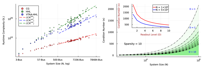
Figure 5: Runtime complexity comparison and potential PQA parameter range. Left: Complexity comparison between CG, HHL-Optimistic and VTAA-HHL-Optimistic for power networks from PGLib[35]. The fit beyond the 500-Bus system indicate that approximate end-to-end runtime complexity of CG is $\mathcal{O}(N^{2.5})$, which is significantly lower than HHL’s $\mathcal{O}(N^{5.5})$ and even VATT-HHL’s end-to-end runtime complexity $\mathcal{O}(N^{4.5})$. Therefore, it is evident that there is no practical quantum advantage in solving DCPF for these systems. Right: Upper bound of condition number ($\kappa$) values for achieving PQA using HHL complexity (4), at different readout levels for system size $N$. Dotted black lines indicate different readout levels and $D=10$ means that only 10 classical values need to be extracted from the solution state $|\mathbf{x}\rangle$. Below these curves, the runtime complexity of CG is worse than that of HHL and there is a possibility of PQA. Importantly, for the PGLib systems we cannot achieve any quantum speedup even for a single readout without reducing the condition number. It is clear from Table 1 and related discussion, that PQA can only be achieved if the condition number is reduced using preconditioning and readout requirements are limited to a fraction of the state vector length. Here complexity dependence on error is ignored considering that errors do not scale with system size. Also, we consider machine overheads to be insignificant.

Figure 5 (right) illustrates the interplay between condition number $\kappa$, system size $N$, and readout level $D$ for attaining PQA, at constant sparsity. Notably, higher readout levels demand lower condition numbers for PQA. In a power system, it is a well-known fact that the number of branches reaching or violating desired limits is only a fraction of the total number of branches. Thus, a problem to identify the power flow on candidate violating branches can be cast as a linear system with very low readout level requirements. However, for PQA, this system would still require preconditioning to reduce the condition number. Therefore, exploring techniques to mitigate condition number growth is essential for achieving PQA. Most importantly, the conditions in Figure 5 highlight the possibility of having PQA with at most sub-quadratic speedup. For near-exponential speedup, both the condition number and readout requirements should ideally not scale with the size of the system.

In conclusion, our end-to-end analysis of QPF complexity reveals a nuanced picture of PQA in power flow calculations. While initial claims of exponential speedups proved illusory, this research pinpoints a narrow window where PQA might be achievable. For DCPF and FDLF problems, our findings demonstrate the absence of PQA under typical network parameters and problem specifications. However, for DCPF-type problems with specific condition number values and readout requirements, a sub-quadratic speedup may be attainable. This highlights the need for further research into tailored QPF algorithms and problem settings to unlock the true potential of quantum computing for power grid analysis. This work provides a critical step towards demystifying the hype surrounding QPF and understanding the requirements for future breakthroughs in this field.

Supplementary Information

Demystifying Quantum Power Flow: Unveiling the Limits of Practical Quantum Advantage

A. Brief Explanation of CG Algorithm

CG iteratively find minimum of $f(\mathbf{x})=\frac{1}{2}\mathbf{x}^{T}A\mathbf{x}-\mathbf{b}^{T}\mathbf{x}+c$, which is a solution of $A\mathbf{x}=\mathbf{b}$ if $A$ is positive definite. The main idea of CG is to generate vectors at each iteration that are conjugate (or A-orthogonal) to all previous iteration vectors and only require $i$-th conjugate vector for generating $i+1$-th conjugate vector[9]. Using the conjugate property of these vectors (called direction vectors), it can be shown that CG will require at most $N$ iterations to converge to the solution of $A\mathbf{x}=\mathbf{b}$, from starting any point $\mathbf{x}^{o}\in\mathbb{R}^{N}$. However, the floating point round-off errors and cancellation errors prevent using CG to find an exact solution. Also, for DCPF problems, we are interested in finding a solution while accepting $\texttt{error}\leq\texttt{Measuring Device Precision}$. In performing these conjugate vector calculations and update states in CG, matrix-vector multiplication becomes the dominant operation [9]. Moreover, For a sparse matrix with at max $s$ non-zero elements in a row, one matrix-vector multiplications will have complexity $\mathcal{O}(Ns)$.

The second part of CG complexity will depend on the number of these matrix-vector multiplications to find the solution $\mathbf{x}^{\star}$ with an acceptable error $\varepsilon_{c}$. This means that the number of iterations required can be calculated based on error convergence after $i$-iterations i.e., the relationship between initial and post $i$-th iteration error. Let initial error vector $\mathbf{e}^{o}=\mathbf{x}^{\star}-\mathbf{x}^{o}$ and after $i$ iterations $\mathbf{e}^{i}=\mathbf{x}^{\star}-\mathbf{x}^{i}$ than error convergence will mean $\|\mathbf{e}^{i}\|_{A}\leq\varepsilon_{c}\|\mathbf{e}^{o}\|_{A}$. Here, $\|\mathbf{e}\|^{2}_{A}=\mathbf{e}^{T}A\mathbf{e}$ is sometimes refereed as energy-norm [9] and $\varepsilon_{c}$ is the error constant which determines how close CG convergence to actual solution, with respect to the initial error ($\varepsilon_{c}\geq\|\mathbf{e}^{i}\|_{A}\big{/}\|\mathbf{e}^{o}\|_{A}$ ). Further, using convergence analysis from [9], maximum number of iterations needed to achieve $\varepsilon_{c}$ given as

$$i\leq\bigg{\lceil}\frac{1}{2}\sqrt{\kappa}\log(2/{\varepsilon_{c}})\bigg{\rceil}$$

The square root dependence of CG runtime complexity on condition number $\kappa$ is beneficial because power system network matrix $A$ tends to have high condition number and approximately quadratic growth of $\kappa$ with respect to system size $N$ for PGLib networks. The feature of power system matrices having high condition numbers affects the convergence of CG as a high condition number implies a higher eigenvalue spread meaning we require a large number of iterations to converge[9]. Preconditioning of linear system $A\mathbf{x}=\mathbf{b}$ can solve this problem. However, finding a computationally cheap and stable preconditioner is a non-trivial problem[9].

For comparing the complexity of CG with HHL-QPF, it’s crucial to establish the relationship between $\varepsilon_{c}$ (error defined using the energy norm) and $\varepsilon$ (error defined using the Euclidean norm). If $A$ is positive semidefinite (PSD) and $\lambda_{1}<\dots<\lambda_{N}$ represents the ordered set of eigenvalues of $A$, then $\lambda_{1}\varepsilon\leq\varepsilon_{c}$. Thus running CG till the energy norm of the error is less than $\varepsilon/\lambda_{1}$ guarantees that the $L_{2}$ error in the solution is less than $\varepsilon$. This unifies the error guarantees of CG and HHL and brings their complexities to the same footing. Additionally, as shown in Fig. 6, for PGLib systems, the smallest eigenvalue grows approximately as $N^{x}$ with $N$ being number of buses. Consequently, the CG complexity in Table I will include a $\log(N)$ term when we substitute $\varepsilon_{c}$ with $\varepsilon$ in the end-to-end complexity.

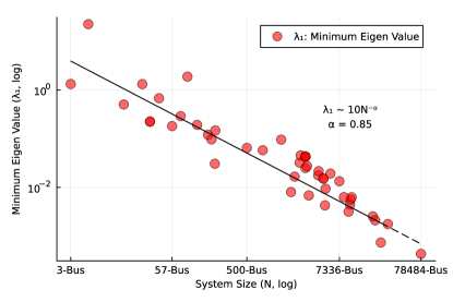
Figure 6: Decay of minimum eigenvalue with system size for PGLib systems [35] (except PEGASE systems).

B. Brief Explanation of HHL

The algorithm commences by encoding the load vector $|b\rangle$ information onto an $n=\log(N)$ qubit register using a unitary operation $U_{b}$ such that $U_{b}|0\rangle=|\mathbf{b}\rangle$. This action signifies that the initial value register is now in a state containing the information from $|\mathbf{b}\rangle$. Subsequently, the quantum phase estimation subroutine is employed to encode the eigenvalues of matrix $A$ into an $n_{c}$-qubit register. The number of qubits ($n_{c}$) determines the accuracy with which the phase values, i.e., eigenvalues, are stored. The next step involves applying controlled rotation to an ancilla register (one qubit) based on the eigenvalues stored in the $n_{c}$-register. This rotation utilizes the principle that for a Hermitian $A$, the eigenvalues of $A^{-1}$ are the inverses of the eigenvalues of $A$, using the spectral decomposition theorem. In other words, if $A=Q\Lambda Q^{\dagger}$ with $Q$ as the eigenvector matrix and $\Lambda$ as the diagonal matrix with eigenvalue entries, then $A^{-1}=Q\Lambda^{-1}Q^{\dagger}$. Upon rotation, the probability of obtaining $|1\rangle$ in the ancilla register outcome, through measurement, is proportional to the eigenvalues of $A^{-1}$, i.e., the inverses of the eigenvalues of $A$. Then an inverse phase estimation is performed to return the $n_{c}$-qubit register to its base state $|0\rangle$ and finally, the ancilla is measured. Now, if the ancilla measurement result is $|1\rangle$ then the algorithm succeeds and we get the solution as a quantum state. Otherwise, the entire process starting from state preparation to ancilla measurement is repeated until the state $|1\rangle$ is achieved. The final quantum state $|\tilde{\mathbf{x}}\rangle$ is proportional to the solution vector $|\mathbf{x}\rangle$. Readers can refer to [13, 37, 11, 10] for details and explanation of HHL workings.

C . Additional Caveats

i) Hot Starting: It is clear that if classical and quantum computing errors are less than a threshold, they have a lesser impact on comparative run-time performance analysis. However, by definition of classical error $\varepsilon_{c}$ it is clear that hot-starting or warm-starting a CG-based DCPF solving algorithm can lead to faster run-times as discussed in the main section. In practical situations, we run multiple DCPFs with load variations within a range. Thus, warm-starting will benefit in reducing the overall time taken by the DCPF running over multiple instances. Although in literature the ideas of warm-starting of quantum algorithms have been presented [43], potential benefits, if any, will require closer scrutiny and dedicated quantum linear system warm-starting methods.

ii) Condition Number limitations: The HHL algorithm (and other variants as well) are shown to be robust when the $A$ matrix is well conditioned i.e. low condition number. However, in a power system, the $A$ matrix condition number grows approximately quadratically with the system size as shown in Figure 3(b). Authors in [23] discuss this limitation on condition number and suggest that pre-conditioning methods can be developed to artificially reduce the condition number of the $A$ matrix. However, there are a few limiting factors which will impact any envisioned benefit from preconditioning:

• Pre-conditioner selection is not a trivial problem. Also, the complexity of preconditioning will modify the overall complexity of the linear system-solving process. To maintain a practical quantum advantage, preconditioning complexity must be less than that of solving the linear system itself. For example $A^{-1}$ is a pre-conditioner of $A$ as $A^{-1}A=\rm I$. However finding $A^{-1}$ is equivalent of solving the linear system $A\mathbf{x}=\mathbf{b}$. Therefore, it is difficult to establish if PQA will exist for power flow problems, without analyzing specific preconditioning algorithm.

• Benefits of preconditioning will be available for both classical and quantum algorithms, given that preconditioning complexity is acceptable as discussed in the aforementioned point. Also, note that HHL’s run-time complexity dependence on condition number $\kappa$ is worse than that of CG’s. This implies condition number reduction will impact only the robustness of QPF methods and unlike to play any role in deciding PQA for QPF.

References

- [1] I. E. Agency, “Net zero by 2050 - a roadmap for the global energy sector - summary for policymakers,” 2021.
- [2] J. J. Grainger and W. D. Stevenson, Power system analysis. McGraw-Hill, 1994.
- [3] B. Stott, J. Jardim, and O. Alsac, “Dc power flow revisited,” IEEE Transactions on Power Systems, vol. 24, no. 3, pp. 1290–1300, 2009.
- [4] J. W. Simpson-Porco, “Lossy dc power flow,” IEEE Transactions on Power Systems, vol. 33, no. 3, pp. 2477–2485, 2018.
- [5] X. Ma, H. Song, M. Hong, J. Wan, Y. Chen, and E. Zak, “The security-constrained commitment and dispatch for midwest iso day-ahead co-optimized energy and ancillary service market,” in 2009 IEEE Power & Energy Society General Meeting, 2009, pp. 1–8.
- [6] MISO, “Real-time energy and operating reserve market software formulations and business logic,” 2022, Business Practices Manual Energy and Operating Reserve Markets Attachment D.
- [7] ——, “Energy and operating reserve markets,” 2022, Business Practices Manual Energy and Operating Reserve Markets.
- [8] ——, “Day-ahead energy and operating reserve market software formulations and business logic,” 2022, Business Practices Manual Energy and Operating Reserve Markets Attachment B.
- [9] J. R. Shewchuk, “An introduction to the conjugate gradient method without the agonizing pain,” 1994.
- [10] A. F. Kockum, A. Soro, L. García-Álvarez, P. Vikstål, T. Douce, G. Johansson, and G. Ferrini, “Lecture notes on quantum computing,” 2023.
- [11] A. Jayakumar, A. Adedoyin, J. Ambrosiano, P. Anisimov, W. Casper, G. Chennupati, C. Coffrin et al., “Quantum algorithm implementations for beginners,” ACM Transactions on Quantum Computing, vol. 3, no. 4, jul 2022.
- [12] A. M. Dalzell, S. McArdle, M. Berta, P. Bienias, C.-F. Chen, A. Gilyén, C. T. Hann, M. J. Kastoryano, E. T. Khabiboulline, A. Kubica et al., “Quantum algorithms: A survey of applications and end-to-end complexities,” arXiv preprint arXiv:2310.03011, 2023.
- [13] A. W. Harrow, A. Hassidim, and S. Lloyd, “Quantum algorithm for linear systems of equations,” Physical review letters, vol. 103, no. 15, p. 150502, 2009.
- [14] A. Ambainis, “Variable time amplitude amplification and a faster quantum algorithm for solving systems of linear equations,” arXiv preprint arXiv:1010.4458, 2010.
- [15] A. M. Childs, R. Kothari, and R. D. Somma, “Quantum algorithm for systems of linear equations with exponentially improved dependence on precision,” SIAM Journal on Computing, vol. 46, no. 6, pp. 1920–1950, 2017.
- [16] S. Aaronson, “Read the fine print,” Nature Physics, vol. 11, no. 4, pp. 291–293, 2015.
- [17] E. Tang, “A quantum-inspired classical algorithm for recommendation systems,” in Proceedings of the 51st annual ACM SIGACT symposium on theory of computing, 2019, pp. 217–228.
- [18] ——, “Quantum principal component analysis only achieves an exponential speedup because of its state preparation assumptions,” Physical Review Letters, vol. 127, no. 6, p. 060503, 2021.
- [19] N.-H. Chia, A. P. Gilyén, T. Li, H.-H. Lin, E. Tang, and C. Wang, “Sampling-based sublinear low-rank matrix arithmetic framework for dequantizing quantum machine learning,” Journal of the ACM, vol. 69, no. 5, pp. 1–72, 2022.
- [20] M. Schuld and F. Petruccione, Supervised learning with quantum computers. Springer, 2018, vol. 17.
- [21] F. Feng, Y. Zhou, and P. Zhang, “Quantum power flow,” IEEE Transactions on Power Systems, vol. 36, no. 4, pp. 3810–3812, 2021.
- [22] R. Eskandarpour, P. Gokhale, A. Khodaei, F. T. Chong, A. Passo, and S. Bahramirad, “Quantum computing for enhancing grid security,” IEEE Transactions on Power Systems, vol. 35, no. 5, pp. 4135–4137, 2020.
- [23] B. Sævarsson, S. Chatzivasileiadis, H. Jóhannsson, and J. Østergaard, “Quantum computing for power flow algorithms: Testing on real quantum computers,” in 11th Bulk Power Systems Dynamics and Control Symposium, 2022.
- [24] J. Liu, H. Zheng, M. Hanada, K. Setia, and D. Wu, “Quantum power flows: From theory to practice,” arXiv preprint arXiv:2211.05728, 2022.
- [25] S. Golestan, M. Habibi, S. M. Mousavi, J. M. Guerrero, and J. C. Vasquez, “Quantum computation in power systems: An overview of recent advances,” Energy Reports, vol. 9, pp. 584–596, 2023.
- [26] D. Vereno, A. Khodaei, C. Neureiter, and S. Lehnhoff, “Exploiting quantum power flow in smart grid co-simulation,” in 2023 11th Workshop on Modelling and Simulation of Cyber-Physical Energy Systems (MSCPES). IEEE, 2023, pp. 1–6.
- [27] Z. Kaseb, M. Moller, G. T. Balducci, P. Palensky, and P. P. Vergara, “Quantum neural networks for power flow analysis,” arXiv preprint arXiv:2311.06293, 2023.
- [28] F. Gao, G. Wu, S. Guo, W. Dai, and F. Shuang, “Solving dc power flow problems using quantum and hybrid algorithms,” Applied Soft Computing, vol. 137, p. 110147, 2023.
- [29] F. Amani, R. Mahroo, and A. Kargarian, “Quantum-enhanced dc optimal power flow,” in 2023 IEEE Texas Power and Energy Conference (TPEC). IEEE, 2023, pp. 1–6.
- [30] F. Feng, Y.-F. Zhou, and P. Zhang, “Noise-resilient quantum power flow,” iEnergy, vol. 2, no. 1, pp. 63–70, 2023.
- [31] D. Neufeld, S. F. Hafshejani, D. Gaur, and R. Benkoczi, “A hybrid quantum algorithm for load flow,” arXiv preprint arXiv:2310.19953, 2023.
- [32] J. Preskill, “Quantum computing and the entanglement frontier,” arXiv preprint arXiv:1203.5813, 2012.
- [33] D. Ristè, M. P. Da Silva, C. A. Ryan, A. W. Cross, A. D. Córcoles, J. A. Smolin, J. M. Gambetta, J. M. Chow, and B. R. Johnson, “Demonstration of quantum advantage in machine learning,” npj Quantum Information, vol. 3, no. 1, p. 16, 2017.
- [34] M. Cramer, M. B. Plenio, S. T. Flammia, R. Somma, D. Gross, S. D. Bartlett, O. Landon-Cardinal, D. Poulin, and Y.-K. Liu, “Efficient quantum state tomography,” Nature communications, vol. 1, no. 1, p. 149, 2010.
- [35] S. Babaeinejadsarookolaee et al., “The power grid library for benchmarking ac optimal power flow algorithms,” arXiv preprint arXiv:1908.02788, 2019.
- [36] L. Lin and Y. Tong, “Optimal polynomial based quantum eigenstate filtering with application to solving quantum linear systems,” Quantum, vol. 4, p. 361, 2020.
- [37] A. Zaman, H. J. Morrell, and H. Y. Wong, “A step-by-step hhl algorithm walkthrough to enhance understanding of critical quantum computing concepts,” IEEE Access, vol. 11, pp. 77 117–77 131, 2023.
- [38] M. Plesch and Č. Brukner, “Quantum-state preparation with universal gate decompositions,” Physical Review A, vol. 83, no. 3, p. 032302, 2011.
- [39] O. Di Matteo, V. Gheorghiu, and M. Mosca, “Fault-tolerant resource estimation of quantum random-access memories,” IEEE Transactions on Quantum Engineering, vol. 1, pp. 1–13, 2020.
- [40] G. Brassard, P. Hoyer, M. Mosca, and A. Tapp, “Quantum amplitude amplification and estimation,” Contemporary Mathematics, vol. 305, pp. 53–74, 2002.
- [41] D. Dervovic, M. Herbster, P. Mountney, S. Severini, N. Usher, and L. Wossnig, “Quantum linear systems algorithms: a primer,” arXiv preprint arXiv:1802.08227, 2018.
- [42] J. van Apeldoorn, A. Cornelissen, A. Gilyén, and G. Nannicini, “Quantum tomography using state-preparation unitaries,” in Proceedings of the 2023 Annual ACM-SIAM Symposium on Discrete Algorithms (SODA). SIAM, 2023, pp. 1265–1318.
- [43] F. Truger, J. Barzen, M. Bechtold, M. Beisel, F. Leymann, A. Mandl, and V. Yussupov, “Warm-starting and quantum computing: A systematic mapping study,” arXiv preprint arXiv:2303.06133, 2023.