The discrete direct deconvolution model in the large eddy simulation of turbulence

Abstract

The discrete direct deconvolution model (D3M) is developed for the large-eddy simulation (LES) of turbulence. The D3M is a discrete approximation of previous direct deconvolution model studied by Chang et al. ["The effect of sub-filter scale dynamics in large eddy simulation of turbulence," Phys. Fluids 34, 095104 (2022)]. For the first type model D3M-1, the original Gaussian filter is approximated by local discrete formulation of different orders, and direct inverse of the discrete filter is applied to reconstruct the unfiltered flow field. The inverse of original Gaussian filter can be also approximated by local discrete formulation, leading to a fully local model D3M-2. Compared to traditional models including the dynamic Smagorinsky model (DSM) and the dynamic mixed model (DMM), the D3M-1 and D3M-2 exhibit much larger correlation coefficients and smaller relative errors in the a priori studies. In the a posteriori validations, both D3M-1 and D3M-2 can accurately predict turbulence statistics, including velocity spectra, probability density functions (PDFs) of sub-filter scale (SFS) stresses and SFS energy flux, as well as time-evolving kinetic energy spectra, momentum thickness, and Reynolds stresses in turbulent mixing layer. Moreover, the proposed model can also well capture spatial structures of the Q-criterion iso-surfaces. Thus, the D3M holds potential as an effective SFS modeling approach in turbulence simulations.

I INTRODUCTION

Large eddy simulation (LES) is an important method for studying turbulence. LES separates large-scale and small-scale motions in turbulence through filtering operations, which solves the large-scale motions directly, and models the effects of small-scale flow structures. This allows more efficient simulation of turbulent flows with limited computational resources, especially for those flow phenomena that are mainly dependent of large-scale motions. One of the prominent challenges in LES is the accurate reconstruction of sub-filter scale (SFS) stresses.Pope (2000); Sagaut (2006) Over the past several decades, various SFS models have been developed,Moser, Haering, and Yalla (2021) including the Smagorinsky model,Smagorinsky (1963) dynamic Smagorinsky model (DSM),Lilly (1992) and dynamic mixed model (DMM).Zang, Dahlburg, and Dahlburg (1992); Vreman, Geurts, and Kuerten (1994) Additionally, implicit LES,Boris et al. (1992); Visbal, Morgan, and Rizzetta (2003); Grinstein, Margolin, and Rider (2007) which does not require explicit SFS modeling but relies on numerical dissipation to capture SFS effects, has emerged as an alternative approach. With the advancement of machine learning, artificial-neural-network-based LES methods have also gained prominence.Duraisamy, Iaccarino, and Xiao (2019); Brunton, Noack, and Koumoutsakos (2020); Kutz (2017); Gamahara and Hattori (2017); Wang et al. (2018a); Schoepplein et al. (2018); Zhou et al. (2019); Yang et al. (2019); Beck, Flad, and Munz (2019); Xie et al. (2019a, b); Xie, Wang, and E (2020); Park and Choi (2021); Li et al. (2021); Novati, de Laroussilhe, and Koumoutsakos (2021); Guan et al. (2022); Wu et al. (2022); Bae and Koumoutsakos (2022); Vadrot, Yang, and Abkar (2023); Kurz, Offenhäuser, and Beck (2023)

In LES, filtering operation separates different scales of motion in turbulence, which helps better understand the nature of turbulence and provides more efficient simulation tools for engineering flow and fluid dynamics research.Pope (2000); Sagaut (2006) Stolz and Adams (1999) showed that the SFS stresses can be approximately reconstructed by iteratively inverting the filtered flow field for an invertible filter. Based on this observation, the approximate deconvolution model (ADM) has been proposed and applied in the incompressible wall-bounded flowsStolz, Adams, and Kleiser (2001a) and the shock-turbulent-boundary-layer interaction.Stolz, Adams, and Kleiser (2001b) The ADM has successful applications in various domains, including the LES of Burgers’ turbulence,Aprovitola and Denaro (2004), turbulent channel flows,Schwertfirm, Mathew, and Manhart (2008) oceanography,San et al. (2011); San, Staples, and Iliescu (2013), magnetohydrodynamics,Labovsky and Trenchea (2010) combustion,Mathew (2002); Domingo and Vervisch (2015, 2017); Mehl, Idier, and Fiorina (2018); Wang and Ihme (2017, 2019); Nikolaou, Cant, and Vervisch (2018); Nikolaou and Vervisch (2018); Seltz et al. (2019); Domingo et al. (2020) and multiphase flow.Schneiderbauer and Saeedipour (2018, 2019); Saeedipour, Vincent, and Pirker (2019) Simulation frameworks based on deconvolution have also been adapted for temporal regularization rather than spatial regularizationPruett (2015), and have also found applications in Lattice-Boltzmann methodsNathen et al. (2018). Mathematical proofs and dedicated literature have also been developed regarding the ADM.Dunca and Epshteyn (2006); Dunca (2012); Layton and Neda (2007); Layton and Stanculescu (2009); Layton and Rebholz (2012); Berselli and Lewandowski (2012); Dunca (2018)

The approximate deconvolution model is primarily based on the van Cittert iteration.Van Cittert (1931); Schlatter, Stolz, and Kleiser (2004); San and Vedula (2018) On the basis of ADM, data-driven deconvolution methods have been developed.Maulik and San (2017); Maulik et al. (2018, 2019); Deng et al. (2019); Liu et al. (2020) The neural networks mapping the filtered and unfiltered fields have been established and applied in various turbulence studies.Maulik and San (2017); Maulik et al. (2018, 2019) A deconvolutional artificial neural network (DANN) model has been proposed,Yuan, Xie, and Wang (2020); Yuan et al. (2021a) where artificial neural network is used to approximate the inverse of the filter. The DANN method has also been extended to model the SFS terms in LES of compressible turbulence with exothermic chemical reactions.Teng, Yuan, and Wang (2022) To address the challenge of neural networks relying on the a priori flow field data, Yuan et al. (2021b) further introduced the dynamic iterative approximate deconvolution (DIAD) model, which has been applied to decaying compressible turbulenceZhang et al. (2022a) and dense gas turbulence.Zhang et al. (2022b)

The selection of filters in LES is also crucial. Geurts (1997) derived analytical expressions for inverting the box filter and utilized these expressions to develop generalized scale-similarity models for the Reynolds stresses tensor. Kuerten et al. (1999) derived an analytical formula for inverting the box filter and employed it in the development of a dynamic stresses-tensor model. Adams, Hickel, and Franz (2004) systematically developed implicit SFS models by recognizing that averaging and reconstruction using a box filter in finite-volume formulations are equivalent to filtering and deconvolution operations. This procedure was subsequently extended to three-dimensional Navier–Stokes equations.Hickel, Adams, and Domaradzki (2006) Boguslawski et al. (2021) utilized inverse Wiener filtering to invert the discrete filter implied by the numerical differentiation, effectively deconvolving the resolved field on the mesh. San, Staples, and Iliescu (2015) conducted an investigation into the effects of different filters on the LES solution by employing 2D and 3D LES of Taylor-Green vortices, and decaying 1D Burger’s turbulence.San (2016) GermanoGermano (1986) introduced a differential filter that has an exact inverse, allowing for the accurate reconstruction of the unfiltered flow field, and further the accurate construction of SFS stresses. Bull and Jameson (2016) applied the inverse Helmholtz filter to reconstruct the SFS stresses in the LES of channel turbulence. Bae and Lozano-Durán (2017, 2019) performed simulations for the turbulent channel flow, where the unfiltered velocities can be obtained by reversing the filter. Chang et al.Chang, Yuan, and Wang (2022) systematically studied the SFS dynamics of the direct deconvolution model (DDM) using nine different invertible filters and evaluated the impact of different filter-to-grid ratios (FGRs) on the DDM prediction accuracy. The DDM gives erroneous predictions at $\mathrm{FGR}=1$, while predicts very accurately at $\mathrm{FGR}=2$. Subsequently, to extend DDM to anisotropic grids, Chang et al.Chang et al. (2023) further investigated the performance of DDM in the case of anisotropic filtration. Under the condition of $\mathrm{FGR}=2$, DDM exhibits high accuracy across a range of anisotropic filter aspect ratios (ARs) from 1 to 16, outperforming traditional DSM and DMM. Sagaut and Grohens (1999) theoretically analyzed these filters in physical space, defined equivalence classes and proposed methods of constructing discrete filters. The study also explores the sensitivity of various SFS models to the test filter, introducing improved versions that consider its spectral width. Supported by the a priori testing with LES turbulence data, the analysis reveals the significant influence of the test filter. Nikolaou, Vervisch, and Domingo (2023) analytically explored reconstruction properties of filters and the impact of discrete approximations on convergence and accuracy. An adaptive optimization framework is proposed to calculate explicit forward and direct-inverse filter coefficients. Optimised filters exhibit stable reconstruction, reducing computational costs for reconstruction in large-eddy simulations.

Our previous research on the DDM has mainly focused on spectral space, where the exact inverse of filter operation can be performed directly. However, spectral methods have limited applicability mainly due to periodic boundary conditions and simple geometry of flow fields.Canuto et al. (2012) We aim to extend the DDM to physical space, leading to the development of the discrete direct deconvolution model (D3M) in this study. Nikolaou, Vervisch, and Domingo (2023) has proposed a constrained and adaptive optimization framework, facilitating the automated computation of explicit forward and direct-inverse discrete filter coefficients based on a predefined filter transfer function. We adopt a similar approach in deriving the forward discrete filters, while the derivation method of the inverse filter is different. Moreover, we focus on the application of the ordinary version of discrete filters to the reconstruction of SFS stresses, and systematically evaluate the accuracy of such SFS models for LES of turbulence. We show that additional artificial dissipation is required to make the D3M approach both stable and accurate in LES. We applied the D3M to homogeneous isotropic turbulence (HIT) and turbulent mixing layer (TML), and evaluate the predictive ability of D3M and traditional models on turbulence statistics and flow field structures through the a priori and a posteriori studies. D3M can be applied in the frameworks of finite difference and finite volume methods, broadening the scope of application for the DDM. For the first type model D3M-1, the original Gaussian filter is approximated by local discrete formulation of different orders, and direct inverse of the discrete filter is applied to reconstruct the unfiltered flow field. The inverse of original Gaussian filter can be also approximated by local discrete formulation, leading to a fully local model D3M-2.

The structure of this article is as follows. Section II first presents the governing equations and the discrete filters. Then the construction of D3M-1 and D3M-2 is introduced. We also introduce the numerical method of turbulence simulations and DNS database. Section III illustrates the a priori results of D3M-1 and D3M-2. Section IV gives the a posteriori results, for LES of two different types of turbulent flows: HIT and TML. Section V summarizes the work presented in this paper.

II GOVERNING EQUATIONS AND NUMERICAL METHODS

Incompressible turbulence follows the Navier-Stokes equations

$$\frac{\partial u_{i}}{\partial x_{i}}=0,$$ (1)

$$\frac{\partial u_{i}}{\partial t}+\frac{\partial(u_{i}u_{j})}{\partial x_{j}}=-\frac{\partial p}{\partial x_{i}}+\nu\frac{\partial^{2}u_{i}}{\partial x_{j}\partial x_{j}}+F_{i}.$$ (2)

In Eqs. 1 and 2, $u_{i}$ denotes the velocity component in the i-th direction, p represents the pressure divided by constant density, $\nu$ denotes the kinematic viscosity, and $F_{i}$ represents the large-scale force in the i-th direction.Yuan, Xie, and Wang (2020) In this paper, unless specifically stated otherwise, repeated indices are assumed to follow the summation convention.

A low-pass filter is applied in the spatial domain, which serves to distinguish the resolved large scales from the sub-filter scales (SFS). For a physical quantity $\phi$, the filtering operation is defined as

$$\bar{\phi}(x)=\int\limits_{\Omega}\phi(x^{\prime})G(x-x^{\prime};\bar{\Delta})dx^{\prime},$$ (3)

where, the overbar denotes spatial filtering and $\Omega$ represents the entire spatial domain. $G$ is the convolution kernel, and $\bar{\Delta}$ is the filter width. Applying the spatial filtering operation to the mass and momentum equations yields the filtered Navier-Stokes equations.

$$\frac{\partial\bar{u}_{i}}{\partial x_{i}}=0,$$ (4)

$$\frac{\partial\bar{u}_{i}}{\partial t}+\frac{\partial(\bar{u}_{i}\bar{u}_{j})}{\partial x_{j}}=-\frac{\partial\bar{p}}{\partial x_{i}}-\frac{\partial\tau_{ij}}{\partial x_{j}}+\nu\frac{\partial^{2}\bar{u}_{i}}{\partial x_{j}\partial x_{j}}+\bar{F}_{i}.$$ (5)

Here, the bar, $\bar{\cdot}$, indicates the filtered variables, while $\tau_{ij}$ are the unclosed SFS stresses, representing the nonlinear effects of SFS flow structures on the large scale dynamics,

$$\tau_{ij}=\overline{u_{i}u_{j}}-\bar{u}_{i}\bar{u}_{j}.$$ (6)

In LES, there are two types of filtering methods: implicit filtering and explicit filtering.Lund (2003) Explicit filtering employs a filter with a known and explicit form. Implicit filtering, on the other hand, involves projecting the governing equations onto a coarser grid, which intrinsically acts as a filtering operation. For further details on this topic, one can refer to additional literature.Boris et al. (1992); Visbal, Morgan, and Rizzetta (2003); Adams, Hickel, and Franz (2004); Grinstein, Margolin, and Rider (2007); Winckelmans et al. (2001); Carati, Winckelmans, and Jeanmart (2001); Domaradzki and Adams (2002); Domaradzki (2010) The present work employs an invertible explicit filtering operation where the form of the filter is known, thus enabling direct deconvolution.Bull and Jameson (2016); Chang, Yuan, and Wang (2022); Chang et al. (2023)

The time advancement is realized through an explicit second-order Adams-Bashforth scheme.Butcher (2016) Taking the ordinary differential equation $da/dt=f$ as an example, the time advancement can be expressed as

$$a^{n+1}=a^{n}+\frac{\Delta t}{2}\left(3f^{n}-f^{n-1}\right)$$ (7)

Here, the superscripts $n$ and $n+1$ represent the current and next time steps, respectively. $a$ is the variable and $f$ is time derivative of $a$. $\Delta t$ is the time step size.

The DDM can be formulated in the following expressionStolz and Adams (1999); Stolz, Adams, and Kleiser (2001a, b); Bull and Jameson (2016); Chang, Yuan, and Wang (2022); Chang et al. (2023)

$$\tau_{ij}=\overline{u_{i}^{*}u_{j}^{*}}-\bar{u}_{i}^{*}\bar{u}_{j}^{*}.$$ (8)

In the above equation, $u_{i}^{*}$ is the unfiltered velocity obtained directly by deconvolution, i.e.,

$$u_{i}^{*}=\mathrm{DDM}(\bar{u}_{i})=G^{-1}\otimes\bar{u}_{i},$$ (9)

where $\bar{u}_{i}$ is the filtered velocity, and $G^{-1}$ is the inverse of filter $G$. $\mathrm{DDM}$ is abbreviation for direct deconvolution model, and $\otimes$ represents the spatial deconvolution operation. In spectral space, the Gaussian filter $\hat{G}=\hat{G}_{1}\times\hat{G}_{2}\times\hat{G}_{3}$, and its spectral space expression isPope (2000)

$$\hat{G}_{i}^{-1}\left(k\right)={\left[\exp\left(-\frac{k^{2}\bar{\Delta}_{i}^{2}}{24}\right)\right]}^{-1},$$ (10)

where the hat, $\hat{\cdot}$, represents the physical quantity in spectral space. The recovered velocity field, $\hat{u}_{i}^{*}$, can be calculated using algebraic multiplication as

$$\hat{u}_{i}^{*}=\hat{G}^{-1}\cdot\bar{\hat{u}}_{i},\;(i=1,\;2,\;3).$$ (11)

To prevent the value of $\hat{G}^{-1}$ from being too large, a maximum limit can be applied, namely,Chang, Yuan, and Wang (2022); Chang et al. (2023)

$$\hat{G}_{i}^{-1}=\min\left\{\hat{G}_{i}^{-1},\zeta^{-1}\right\},\;\zeta=0.01.$$ (12)

Once $\hat{G}^{-1}$ exceeds this limit $\zeta^{-1}$, it is reset to the maximum value to prevent further growth.

The one-dimensional Gaussian filter in physical space takes the form ofPope (2000)

$$G_{i}(r)=\left(\frac{6}{\pi\bar{\Delta}_{i}^{2}}\right)^{1/2}\exp\left(-\frac{6r^{2}}{\bar{\Delta}_{i}^{2}}\right).$$ (13)

With the help of Taylor expansion, the Gaussian filter can be expanded as follows:Sagaut and Grohens (1999); Nikolaou, Vervisch, and Domingo (2023)

$$\bar{\phi}(x)=\phi(x)+\frac{\bar{\Delta}^{2}}{24}\frac{\partial^{2}\phi(x)}{\partial\xi^{2}}+\frac{\bar{\Delta}^{4}}{1152}\frac{\partial^{4}\phi(x)}{\partial\xi^{4}}+\frac{\bar{\Delta}^{6}}{82944}\frac{\partial^{6}\phi(x)}{\partial\xi^{6}}+\frac{\bar{\Delta}^{8}}{7962624}\frac{\partial^{8}\phi(x)}{\partial\xi^{8}}+O(\bar{\Delta}^{10}).$$ (14)

Accordingly, the discrete filtering operator $G$ is

$$G=1+\frac{\bar{\Delta}^{2}}{24}\frac{\partial^{2}}{\partial x^{2}}+\frac{\bar{\Delta}^{4}}{1152}\frac{\partial^{4}}{\partial x^{4}}+\frac{\bar{\Delta}^{6}}{82944}\frac{\partial^{6}}{\partial x^{6}}+\frac{\bar{\Delta}^{8}}{7962624}\frac{\partial^{8}}{\partial x^{8}}+O\left(\bar{\Delta}^{10}\right).$$ (15)

By discretizing Eq. 14, the global Gaussian filter can be approximated as a local discrete filter,Sagaut and Grohens (1999); Nikolaou, Vervisch, and Domingo (2023) namely,

$$\bar{\phi}_{j}=\sum_{m=-\frac{N}{2}}^{\frac{N}{2}}a_{m}\phi_{j+m},$$ (16)

where $\phi$ represents a physical quantity, and $a_{m}$ is the coefficient. The subscript $j$ denotes the index of the grid point, not the component in the $j$th-direction. The expressions for the discrete Gaussian filter to the different orders of accuracy are given in Table 1.Sagaut and Grohens (1999); Nikolaou, Vervisch, and Domingo (2023)

Table 1: The discrete filters with different order of accuracy for both D3M-1 and D3M-2.

Order of accuracy	Expression
2	$\bar{\phi}_{j}=\frac{1}{24}\alpha^{2}\left(\phi_{j+1}+\phi_{j-1}\right)+\frac{1}{12}\left(12-\alpha^{2}\right)\phi_{j}$
4	$\begin{aligned} \bar{\phi}_{j}=\frac{\alpha^{4}-4\alpha^{2}}{1152}\left(\phi_{j+2}+\phi_{j-2}\right)+\frac{-\alpha^{4}+16\alpha^{2}}{288}\left(\phi_{j+1}+\phi_{j-1}\right)+\frac{\alpha^{4}-20\alpha^{2}+192}{192}\phi_{j}\end{aligned}$
6	$\begin{aligned} \bar{\phi}_{j}=&\frac{5\alpha^{6}-60\alpha^{4}+192\alpha^{2}}{414720}\left(\phi_{j+3}+\phi_{j-3}\right)\\ &+\frac{-5\alpha^{6}+120\alpha^{4}-432\alpha^{2}}{69120}\left(\phi_{j+2}+\phi_{j-2}\right)\\ &+\frac{5\alpha^{6}-156\alpha^{4}+1728\alpha^{2}}{27648}\left(\phi_{j+1}+\phi_{j-1}\right)\\ &+\frac{-5\alpha^{6}+168\alpha^{4}-2352\alpha^{2}+20736}{20736}{\phi_{j}}\end{aligned}$
8	$\begin{aligned} \bar{\phi}_{j}=&\frac{35\alpha^{8}-840\alpha^{6}+7056\alpha^{4}-20736\alpha^{2}}{278691840}\left(\phi_{j+4}+\phi_{j-4}\right)\\ &+\frac{-35\alpha^{8}+1260\alpha^{6}-12096\alpha^{4}+36864\alpha^{2}}{34836480}\left(\phi_{j+3}+\phi_{j-3}\right)\\ &+\frac{35\alpha^{8}-1560\alpha^{6}+24336\alpha^{4}-82944\alpha^{2}}{9253280}\left(\phi_{j+2}+\phi_{j-2}\right)\\ &+\frac{-35\alpha^{8}+1740\alpha^{6}-35136\alpha^{4}+331776\alpha^{2}}{4976640}\left(\phi_{j+1}+\phi_{j-1}\right)\\ &+\frac{35\alpha^{8}-1800\alpha^{6}+39312\alpha^{4}-472320\alpha^{2}+3981312}{3981312}\phi_{j}\end{aligned}$

$\alpha=\bar{\Delta}_{i}/h_{i}^{LES}$ is the FGR, where $\bar{\Delta}_{i}$ is the filtering width in the i-th direction, and $h_{i}^{LES}$ is the grid spacing of the LES. For more details of the discrete filters, see Appendix A.

The comparison between different-order discrete filters and exact Gaussian filters is shown in Fig. 1. Here, $\alpha=1$, 2, and 4. $k_{c}$ denotes the wavenumber corresponding to the grid space, i.e., $k_{c}=\frac{2\pi}{h_{LES}}$. With the order increasing, the shape of the discrete filter gradually approximates that of the exact Gaussian filter. When $\mathrm{FGR}=4$, only the eighth-order filter is suitable for use, as the values of the discrete filters in other orders will exceed the range of $[0,\ 1]$, leading to numerical instability.

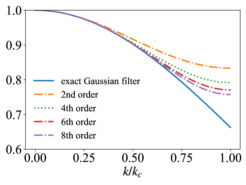
(a)

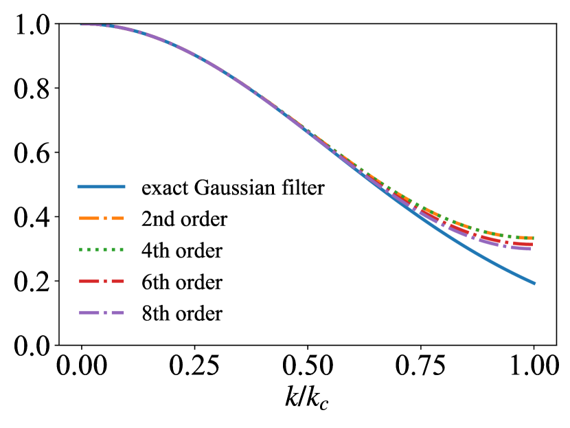
(b)

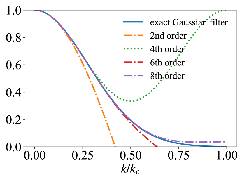
(c)

Figure 1: The comparisons of the discrete filters and the exact Gaussian filter: (a) $\mathrm{FGR}=1$, (b) $\mathrm{FGR}=2$, and (c) $\mathrm{FGR}=4$.

Through Fourier transformation, the expression of discrete filter spectral space can be obtained.

$$\hat{G}_{i}(\kappa) =\sum_{m=-N/2}^{N/2}e^{-\underline{i}\kappa r_{m}}a_{m},$$ (17)

$$=a_{0}+\sum_{m=1}^{N/2}2\cos(m\kappa\bar{\Delta})a_{m}.$$

Note that the superscript, $\underline{i}$ denotes the imaginary unit, whereas the subscript, $i$, denotes the component in the $i$-th direction. $N$ represents the order of the discrete filter. The details of the coefficients, $a_{m}$, can be found in Table 9.Nikolaou, Vervisch, and Domingo (2023) Since the filters are invertible, the inverse of the discrete filters are as follows

$$\hat{G}_{i}^{-1}(\kappa)=\frac{1}{a_{0}+\sum_{m=1}^{N/2}2\cos(m\kappa\bar{\Delta})a_{m}}.$$ (18)

Using Eq. 18, the D3M-1 can be constructed, namely,

$$\hat{u}_{i}^{*}=(\mathrm{D3M\mbox{-}1})(\bar{\hat{u}}_{i})=\hat{G}^{-1}\cdot\bar{\hat{u}}_{i}.$$ (19)

For the first type model D3M-1, the original Gaussian filter is approximated by a local discrete formulation of different orders, and direct inverse of the discrete filter is applied to reconstruct the unfiltered flow field. The inverse of a discrete filter in physical space needs to be obtained by solving a linear system of equations. If it needs to be applied more easily in physical space, further derivations are required, namely, D3M-2.

The inverse of original Gaussian filter can be also approximated by a local discrete formulation, leading to a fully local model D3M-2, namely,Nikolaou, Vervisch, and Domingo (2023)

$$u_{j}^{*}=(\mathrm{D3M\mbox{-}2})(\bar{u})=\sum_{m=-\frac{N}{2}}^{\frac{N}{2}}a_{m}\bar{u}_{j+m},$$ (20)

where the subscript $j$ denotes the index of the grid point, not the component in the $j$th-direction. $N$ represents the order of the discrete filter. The detailed coefficients, $a_{m}$ can be found in Table 10 in Appendix A.

In the spectral space,

$$\hat{u}_{i}^{*}=(\mathrm{D3M\mbox{-}2})(\bar{\hat{u}}_{i})=\hat{G}^{-1}\cdot\bar{\hat{u}}_{i},$$ (21)

where

$$\hat{G}_{i}^{-1}(\kappa) =\sum_{m=-N/2}^{N/2}e^{-\underline{i}\kappa r_{m}}a_{m},$$ (22)

$$=a_{0}+\sum_{m=1}^{N/2}2\cos(m\kappa\bar{\Delta})a_{m},$$

and the details of the coefficients, $a_{m}$, can be found in Table 10.

We choose the second-order discrete filter to elaborate the derivations. Assume the inverse of the filter $G$ exists, then

$$\phi^{*}=G^{-1}\otimes\bar{\phi},$$ (23)

$$G^{-1}=[I-(I-G)]^{-1}.$$ (24)

$(1-x)^{-1}$ can be expanded asSpivak (2006)

$$\frac{1}{1-x}=1+x+x^{2}+\cdots+x^{n}+\cdots,\quad(-1<x<1).$$ (25)

Therefore,

$$G^{-1}=\sum_{p=0}^{\infty}(I-G)^{p}.$$ (26)

Let $p=4$, (equivalent to the fourth-order ADM)Stolz and Adams (1999),

$$G^{-1} =1+(1-G)+(1-G)^{2}+(1-G)^{3}+(1-G)^{4}$$ (27)

$$=5-10G+10G^{2}-5G^{3}+G^{4}.$$

Substitute the Gaussian filter Eqs. 27 and 15 back to Eq. 23.

$$\phi^{*} =G^{-1}\otimes\bar{\phi}$$ (28)

$$=\left(5-10G+10G^{2}-5G^{3}+G^{4}\right)\otimes\bar{\phi}$$

$$=\left[1-\frac{\bar{\Delta}^{2}}{24}\frac{\partial^{2}}{\partial x^{2}}+\frac{\bar{\Delta}^{4}}{1152}\frac{\partial^{4}}{\partial x^{4}}-\frac{\bar{\Delta}^{6}}{82944}\frac{\partial^{6}}{\partial x^{6}}+\frac{\bar{\Delta}^{8}}{7962624}\frac{\partial^{8}}{\partial x^{8}}+O\left(\bar{\Delta}^{10}\right)\right]\bar{\phi}.$$

Then, truncate Eq. 28 to the second-order accuracy,

$$\phi^{*}=\bar{\phi}(x)-\frac{\bar{\Delta}^{2}}{24}\frac{\partial^{2}\bar{\phi}(x)}{\partial x^{2}}+O\left(\bar{\Delta}^{4}\right).$$ (29)

Assume that

$$\phi_{j}^{*}=a_{-1}\bar{\phi}_{j-1}+a_{0}\bar{\phi}_{j}+a_{1}\bar{\phi}_{j+1}.$$ (30)

According to the Taylor’s expansion, we have

$$\bar{\phi}_{j-1}= \bar{\phi}_{j}+\left(-\frac{\bar{\Delta}}{\alpha}\right)\frac{\partial\bar{\phi}_{j}}{\partial x}+\left(-\frac{\bar{\Delta}}{\alpha}\right)^{2}\frac{1}{2!}\frac{\partial^{2}\bar{\phi}_{j}}{\partial x^{2}}+O\left(\bar{\Delta}^{3}\right),$$ (31)

$$= \bar{\phi}_{j}-\frac{\bar{\Delta}}{\alpha}\frac{\partial\bar{\phi}_{j}}{\partial x}+\frac{1}{2}\frac{\bar{\Delta}^{2}}{\alpha^{2}}\frac{\partial^{2}\bar{\phi}_{j}}{\partial x^{2}}+O\left(\bar{\Delta}^{3}\right).$$

$$\bar{\phi}_{j+1}= \bar{\phi}_{j}+\left(\frac{\bar{\Delta}}{\alpha}\right)\frac{\partial\bar{\phi}_{j}}{\partial x}+\left(\frac{\bar{\Delta}}{\alpha}\right)^{2}\frac{1}{2!}\frac{\partial^{2}\bar{\phi}_{j}}{\partial x^{2}}+O\left(\bar{\Delta}^{3}\right),$$ (32)

$$= \bar{\phi}_{j}+\frac{\bar{\Delta}}{\alpha}\frac{\partial\bar{\phi}_{j}}{\partial x}+\frac{1}{2}\frac{\bar{\Delta}^{2}}{\alpha^{2}}\frac{\partial^{2}\bar{\phi}_{j}}{\partial x^{2}}+O\left(\bar{\Delta}^{3}\right).$$

Substitute Eqs. 31 and 32 into Eq. 30, we obtain

$${\phi}_{j}^{*}= (a_{-1}+a_{0}+a_{1})\bar{\phi}_{j}$$ (33)

$$+\left(-a_{-1}+a_{1}\right)\frac{\bar{\Delta}}{\alpha}\frac{\partial\bar{\phi}_{j}}{\partial x}$$

$$+\frac{1}{2}\left(a_{-1}+a_{1}\right)\frac{\bar{\Delta}^{2}}{\alpha^{2}}\frac{\partial^{2}\bar{\phi}_{j}}{\partial x^{2}}.$$

Compare Eq. 33 and Eq. 29, we get

$$a_{-1}+a_{0}+a_{1} =1,$$ (34)

$$(-a_{-1}+a_{1})\frac{\bar{\Delta}}{\alpha} =0,$$

$$\frac{1}{2}(a_{-1}+a_{1})\frac{\bar{\Delta}^{2}}{\alpha^{2}} =-\frac{\bar{\Delta}^{2}}{24}.$$

Solve Eq. 34, we can get

$$a_{-1}=-\frac{\alpha^{2}}{24},a_{0}=\frac{12+\alpha^{2}}{12},a_{1}=-\frac{\alpha^{2}}{24}.$$ (35)

Substitute Eq. 35 back into Eq. 30, the inverse of the discrete Gaussian filter to the second-order is

$$\phi_{j}^{*}=-\frac{1}{24}\alpha^{2}\left(\bar{\phi}_{j+1}+\bar{\phi}_{j-1}\right)+\frac{1}{12}\left(12+\alpha^{2}\right)\bar{\phi}_{j}.$$ (36)

The derivation of discrete filters of other orders are similar, and the expressions are given in Table 2. See Appendix A for details.

Table 2: The discrete inverse filters with different order of accuracy for D3M-2.

Order of accuracy	Expression
2	$\phi_{j}^{*}=-\frac{1}{24}\alpha^{2}\left(\bar{\phi}_{j+1}+\bar{\phi}_{j-1}\right)+\frac{1}{12}\left(12+\alpha^{2}\right)\bar{\phi}_{j}$
4	$\begin{aligned} \phi_{j}^{*}=\frac{\alpha^{4}+4\alpha^{2}}{1152}\left(\bar{\phi}_{j+2}+\bar{\phi}_{j-2}\right)+\frac{-\alpha^{4}-16\alpha^{2}}{288}\left(\bar{\phi}_{j+1}+\bar{\phi}_{j-1}\right)+\frac{\alpha^{4}+20\alpha^{2}+192}{192}\bar{\phi}_{j}\end{aligned}$
6	$\begin{aligned} \phi_{j}^{*}=&\frac{-5\alpha^{6}-60\alpha^{4}-192\alpha^{2}}{414720}\left(\bar{\phi}_{j+3}+\bar{\phi}_{j-3}\right)\\ &+\frac{5\alpha^{6}+120\alpha^{4}+432\alpha^{2}}{69120}\left(\bar{\phi}_{j+2}+\bar{\phi}_{j-2}\right)\\ &+\frac{-5\alpha^{6}-156\alpha^{4}-1728\alpha^{2}}{27648}\left(\bar{\phi}_{j+1}+\bar{\phi}_{j-1}\right)\\ &+\frac{5\alpha^{6}+168\alpha^{4}+2352\alpha^{2}+20736}{20736}{\bar{\phi}_{j}}\end{aligned}$
8	$\begin{aligned} \phi_{j}^{*}=&\frac{35\alpha^{8}+840\alpha^{6}+7056\alpha^{4}+20736\alpha^{2}}{278691840}\left(\bar{\phi}_{j+4}+\bar{\phi}_{j-4}\right)\\ &+\frac{-35\alpha^{8}-1260\alpha^{6}-12096\alpha^{4}-36864\alpha^{2}}{34836480}\left(\bar{\phi}_{j+3}+\bar{\phi}_{j-3}\right)\\ &+\frac{35\alpha^{8}+1560\alpha^{6}+24336\alpha^{4}+82944\alpha^{2}}{9253280}\left(\bar{\phi}_{j+2}+\bar{\phi}_{j-2}\right)\\ &+\frac{-35\alpha^{8}-1740\alpha^{6}-35136\alpha^{4}-331776\alpha^{2}}{4976640}\left(\bar{\phi}_{j+1}+\bar{\phi}_{j-1}\right)\\ &+\frac{35\alpha^{8}+1800\alpha^{6}+39312\alpha^{4}+472320\alpha^{2}+3981312}{3981312}\bar{\phi}_{j}\end{aligned}$

Fig. 2 presents the shapes of inverse filters in D3M-1 and D3M-2. When $\mathrm{FGR}=1$, the results of D3M-1 and D3M-2 are similar. However, at $\mathrm{FGR}=2$, the results of D3M-2 are lower than those of D3M-1. At $\mathrm{FGR}=4$ numerical instability occurs in D3M-1 for second, fourth and sixth orders, while D3M-2 is always positive and stable.

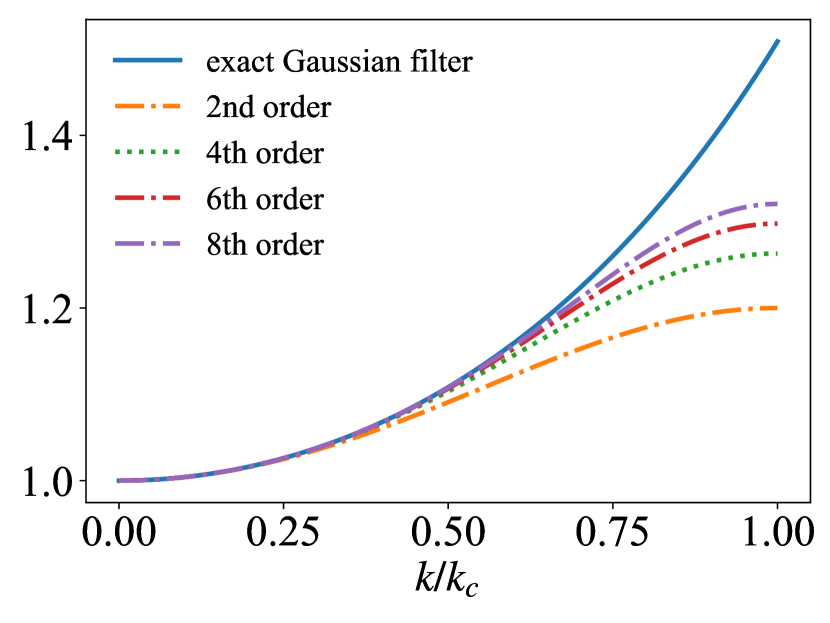
(a)

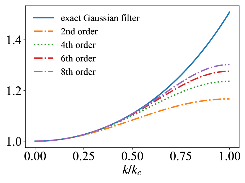
(b)

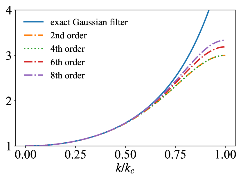
(c)

(d)

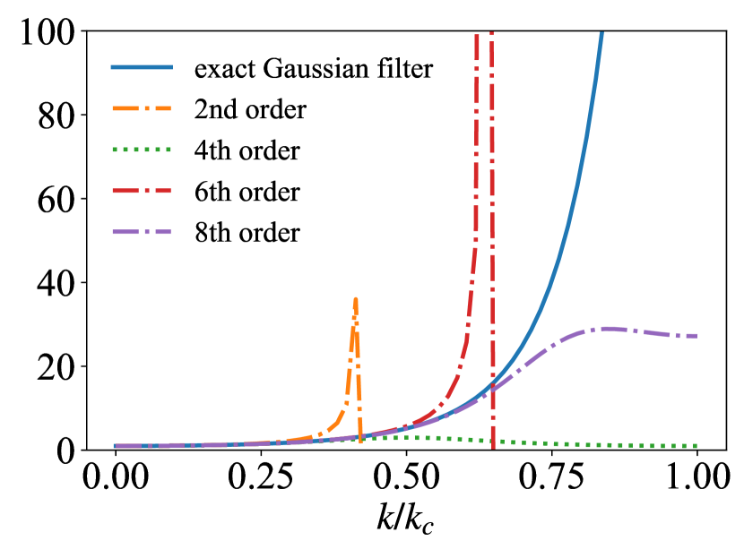
(e)

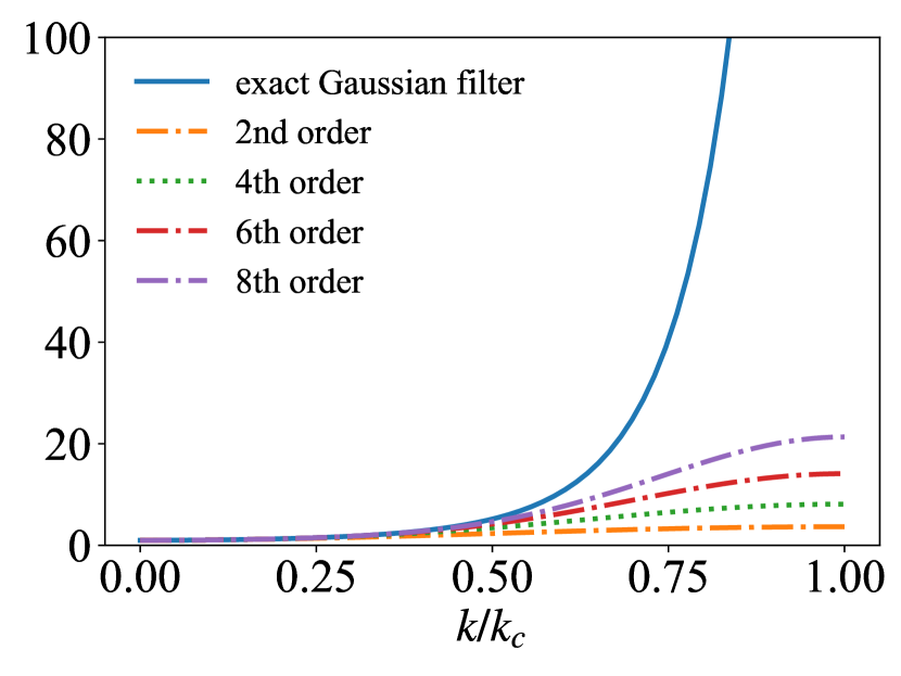
(f)

Figure 2: The comparison of the inverse of discrete filters and the inverse of exact Gaussian filter: (a) D3M-1 at $\mathrm{FGR}=1$, (b) D3M-2 at $\mathrm{FGR}=1$, (c) D3M-1 at $\mathrm{FGR}=2$, (d) D3M-2 at $\mathrm{FGR}=2$, (e) D3M-1 at $\mathrm{FGR}=4$, and (f) D3M-2 at $\mathrm{FGR}=4$.

In the a priori analysis, the DNS data is filtered to obtain a large scale velocity field and true SFS stresses. Then, the filtered velocity field is input into the SFS model to obtain the predicted SFS stresses. Finally, the predicted SFS stresses are then compared with the actual SFS stresses to evaluate the SFS model.Sagaut (2006)

In the a posteriori validation, a complete LES calculation is performed, and then the statistics of the LES and the filtered DNS are compared. The a posteriori analysis is a comprehensive verification method that considers model errors, discretization errors, and numerical scheme errors. Compared to the a priori analysis, it can more comprehensively reflect the true performance of model.Sagaut (2006)

III A PRIORI STUDY OF DIFFERENT SFS MODELS

To evaluate different SFS models, for any physical quantity $Q$, two metrics are employed to assess the discrepancy between the predicted values $Q^{model}$ and the true values $Q^{real}$. These two metrics are the correlation coefficient and the relative error, whose expressions are as follows.Xie et al. (2019a); Yuan, Xie, and Wang (2020)

$$C(Q)=\frac{\langle(Q^{real}-\langle Q^{real}\rangle)(Q^{model}-\langle Q^{model}\rangle)\rangle}{\langle(Q^{real}-\langle Q^{real}\rangle)^{2}\rangle^{1/2}\langle(Q^{model}-\langle Q^{model}\rangle)^{2}\rangle^{1/2}},$$ (37)

$$E_{r}(Q)=\frac{\langle(Q^{real}-Q^{model})^{2}\rangle^{1/2}}{\langle(Q^{real})^{2}\rangle^{1/2}},$$ (38)

where the angle brackets $\langle\cdot\rangle$ represent spatial averaging over the entire computational domain. An accurate model is expected to exhibit high correlation coefficients and low relative errors.

We first use an exact Gaussian filter to filter the DNS data to obtain the true SFS stresses, $\tau_{ij}^{real}$. Simultaneously, we downsample the DNS results using a spectral cutoff filter to approximate the effect of grid discretization. The grid spacings selected are $h_{LES}=8h_{DNS}$ and $h_{LES}=16h_{DNS}$. The corresponding filter widths are set as $\bar{\Delta}=16h_{DNS}$ and $\bar{\Delta}=32h_{DNS}$, respectively, to ensure $\mathrm{FGR}=2$. We use discrete Gaussian filters of different orders to filter the coarsened DNS data, and then substitute filtered data into the SFS model to obtain the predicted SFS stresses modeled by SFS models, $\tau_{ij}^{model}$. By comparing $\tau_{ij}^{real}$ and $\tau_{ij}^{model}$, we can obtain the correlation coefficient and relative error of the SFS model.

In the current study, we conducted a DNS of HIT with Taylor-Reynolds number of 250. The computational domain is a cubic domain of $2\pi$, using periodic boundary conditions. The DNS employs a grid resolution of $1024^{3}$, and Table 3 gives the parameters of the DNS. The Reynolds number is defined by $Re=\frac{U_{ref}L_{ref}}{\nu}$, where $U_{ref}$ is the dimensionless reference velocity, $L_{ref}$ is the dimensionless length scale of the flow field, and $\nu$ is the viscosity of the fluid. The Reynolds number for the Taylor microscale, denoted as $\mathrm{Re}_{\lambda}$, is determined by

$$\mathrm{Re}_{\lambda}=\frac{u^{rms}\lambda}{\sqrt{3}\nu}.$$ (39)

In Eq. 39, $\lambda=u^{rms}\sqrt{5\nu/\epsilon}$ represents the Taylor microscale, where $u^{rms}$ denotes the root mean square (rms) value of the velocity magnitude. $\epsilon$ denotes the dissipation rate, defined as $\epsilon=2\nu\langle S_{ij}S_{ij}\rangle$, with $S_{ij}$ being the strain-rate tensor defined as $S_{ij}=\frac{1}{2}(\partial u_{i}/\partial x_{j}+\partial u_{j}/\partial x_{i})$. The angular brackets, $\langle\cdot\rangle$, denote spatial averaging across the entire computational domain. The total kinetic energy, denoted as $E_{k}$, is given by

$$E_{k}=\frac{1}{2}\langle u_{i}u_{i}\rangle=\int_{0}^{+\infty}E(k)dk,$$ (40)

where $E(k)$ represents the spectrum of kinetic energy per unit mass.Pope (2000) Two crucial characteristic turbulent length scales include the Kolmogorov length scale ($\eta$) and the integral length scale ($L_{I}$), expressed as followsPope (2000)

$$\eta=\Big{(}\frac{\nu^{3}}{\epsilon}\Big{)}^{1/4},$$ (41)

and

$$L_{I}=\frac{3\pi}{2(u^{rms})^{2}}\int_{0}^{+\infty}\frac{E(k)}{k}dk,$$ (42)

respectively. In order to evaluate whether the grid resolution is sufficient, criterion $k_{max}\eta$ is used. $k_{max}=\frac{2\pi}{3h_{DNS}}$ represents the maximum resolvable scale of the DNS. $k_{max}\eta\geq 2.1$ in our simulation indicating that the grid resolution is sufficient to obtain converged kinetic energy spectrum at different scales.Ishihara et al. (2007); Ishihara, Gotoh, and Kaneda (2009) $h_{DNS}=\frac{2\pi}{1024}$ is the grid spacing of the DNS. The rms value of the vorticity magnitude is defined by $\omega^{rms}=\sqrt{\langle\omega_{i}\omega_{i}\rangle}$, where the vorticity is defined as $\mathbf{\omega}=\nabla\times\mathbf{u}$, i.e., the curl of the velocity field.

Table 3: Parameters and statistics for DNS of HIT at grid resolution of $1024^{3}$

$Re$	$Re_{\lambda}$	$E_{k}$	$k_{max}\eta$	$\eta/h_{DNS}$	$L_{I}/\eta$	$\lambda/\eta$	$u^{rms}$	$\omega^{rms}$	$\epsilon$
1000	252	2.63	2.11	1.01	235.2	31.2	2.30	26.90	0.77

The flow field is driven by large-scale forces, and the energy spectrum values at the first two wave numbers are set to fixed values. Then a coefficient, $\gamma$, is multiplied by the velocity component to obtain the forced velocity component. The expression is:Wang et al. (2012a, 2020, b, 2018b)

$$\hat{u}_{j}^{f}(\mathbf{k})=\gamma\hat{u}_{j}(\mathbf{k}),where\;\gamma=\begin{cases}\sqrt{E_{0}(1)/E_{k}(1)},&\,0.5\leq k\leq 1.5\\ \sqrt{E_{0}(2)/E_{k}(2)},&\,1.5\leq k\leq 2.5\\ 1,&\,\mathrm{otherwise}.\end{cases}$$ (43)

The range of the energy spectra defined for the first two wave numbers is specified as follows. $E_{k}(1)$ and $E_{k}(2)$ correspond to wavenumbers within the range $0.5\leq k\leq 1.5$ and $1.5\leq k\leq 2.5$, respectively. $E_{k}(1)$ and $E_{k}(2)$ are calculated as $E_{k}(1)=\int_{0.5}^{1.5}E(k)dk$ and $E_{k}(2)=\int_{1.5}^{2.5}E(k)dk$, respectively. The kinetic energy spectra are set as $E_{0}(1)=1.242477$ and $E_{0}(2)=0.391356$. As the first two forced wavenumbers are far away from the filtering scale, the influence of the forcing on the filtering scale can be neglected.

The detailed results of the a priori study are recorded in Tables 4 and 5. At $\bar{\Delta}=16h_{DNS}$, the D3M-1 and D3M-2 have better accuracy than the traditional VGM, DSM, and DMM. For each SFS model, as the filter order increases, the correlation coefficients increase and the relative errors decrease. At the same order, D3M-1 has slightly higher correlation coefficients and lower correlation errors compared to D3M-2. As the order of the discrete filter continues to increase, the accuracy of D3M-1 and D3M-2 continuously approaches towards the accuracy of DDM. At $\bar{\Delta}=32h_{DNS}$, the trend of the a priori results is similar to that at $\bar{\Delta}=16h_{DNS}$, where both D3M-1 and D3M-2 have correlation coefficients higher than 94%, and relative errors lower than 40%, which are superior to those of DSM and DMM.

Table 4: The correlation coefficients ($C$) and relative errors ($E_{r}$) for discrete filters with different order of accuracy at filter width $\bar{\Delta}=16h_{DNS}$

. Models Order of the filter $C(\tau_{11},\ \tau_{12})$ $E_{r}(\tau_{11},\ \tau_{12})$ VGM $\cdots$ (0.947, 0.946) (0.333, 0.333) DSM 2 (0.212, 0.221) (1.117, 1.114) 4 (0.212, 0.221) (1.117, 1.114) 6 (0.224, 0.234) (1.068, 1.066) 8 (0.237, 0.247) (1.020, 1.017) exact Gaussian filter (0.249, 0.260) (0.971, 0.969) DMM 2 (0.568, 0.563) (0.864, 0.867) 4 (0.568, 0.563) (0.864, 0.867) 6 (0.601, 0.596) (0.826, 0.829) 8 (0.635, 0.629) (0.789, 0.792) exact Gaussian filter (0.668, 0.662) (0.751, 0.754) DDM exact Gaussian filter (0.990, 0.992) (0.136, 0.125) D3M-1 2 (0.953, 0.955) (0.238, 0.219) 4 (0.953, 0.955) (0.238, 0.219) 6 (0.965, 0.968) (0.211, 0.194) 8 (0.976, 0.978) (0.184, 0.169) D3M-2 2 (0.950, 0.952) (0.245, 0.225) 4 (0.952, 0.954) (0.239, 0.220) 6 (0.960, 0.962) (0.224, 0.206) 8 (0.967, 0.969) (0.204, 0.188)

Table 5: The correlation coefficients ($C$) and relative errors ($E_{r}$) for discrete filters with different order of accuracy at filter width $\bar{\Delta}=32h_{DNS}$

. Models Order of the filter $C(\tau_{11},\ \tau_{12})$ $E_{r}(\tau_{11},\ \tau_{12})$ VGM $\cdots$ (0.912, 0.912) (0.427, 0.425) DSM 2 (0.240, 0.269) (1.112, 1.091) 4 (0.240, 0.269) (1.112, 1.091) 6 (0.254, 0.285) (1.064, 1.044) 8 (0.268, 0.301) (1.015, 0.996) exact Gaussian filter (0.282, 0.317) (0.967, 0.949) DMM 2 (0.533, 0.543) (0.902, 0.887) 4 (0.533, 0.543) (0.902, 0.887) 6 (0.564, 0.575) (0.862, 0.848) 8 (0.596, 0.607) (0.823, 0.810) exact Gaussian filter (0.627, 0.639) (0.784, 0.771) DDM exact Gaussian filter (0.975, 0.978) (0.223, 0.212) D3M-1 2 (0.939, 0.942) (0.390, 0.371) 4 (0.939, 0.942) (0.390, 0.371) 6 (0.951, 0.955) (0.346, 0.329) 8 (0.961, 0.964) (0.301, 0.286) D3M-2 2 (0.936, 0.939) (0.401, 0.382) 4 (0.938, 0.941) (0.392, 0.373) 6 (0.946, 0.949) (0.368, 0.350) 8 (0.953, 0.956) (0.335, 0.318)

Fig. 3 presents the correlation coefficients and relative errors of different models at the filter width of $\bar{\Delta}=32h_{DNS}$. As the order increases, the correlation coefficient decreases, and the relative error increases. Overall, the results of D3M-1 and D3M-2 are similar, with correlation coefficients higher than those of DSM and DMM, and relative errors lower than those of DSM and DMM.

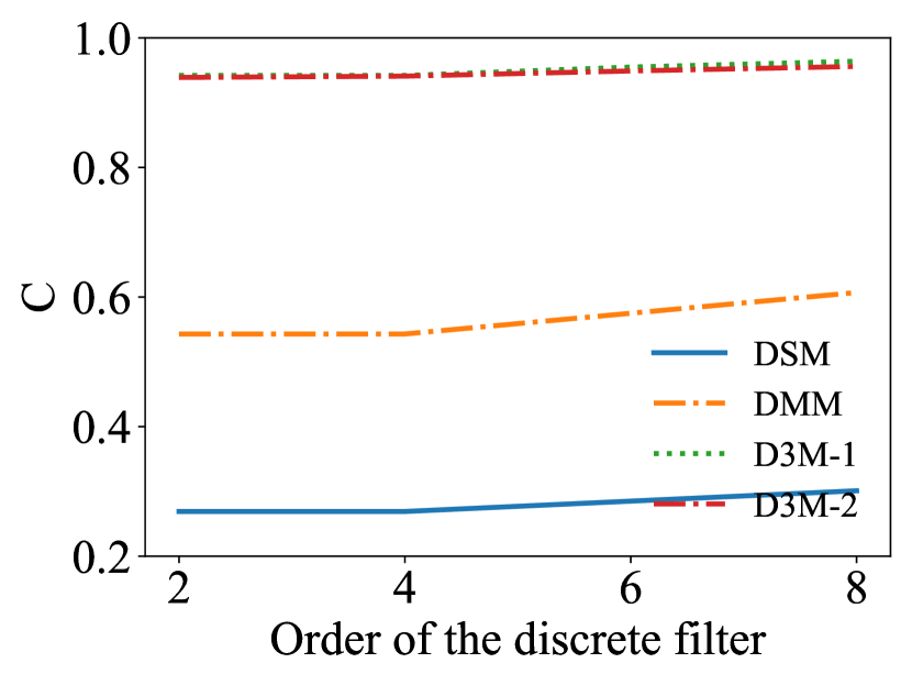
(a)

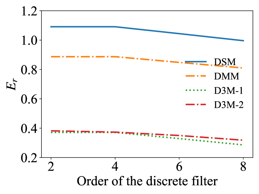
(b)

Figure 3: Correlation coefficients and relative errors of shear components of the SFS stresses $\tau_{12}^{A}$ for different models with multiple orders of discrete filter at filter width $\bar{\Delta}=32h_{DNS}$ in the a priori study: (a) correlation coefficients C and (b) relative errors $E_{r}$.

IV A POSTERIORI STUDY of LES

The a posteriori tests are indispensable for the SFS models, as they consider practical factors including errors from both numerical discretization schemes and the model itself, making it more comprehensive than the a priori tests.Lesieur and Metais (1996); Meneveau and Katz (2000) Four SFS models are used in the a posteriori tests: DSM, DMM, D3M-1, and D3M-2. Appendix C gives the detailed expressions of the DSM and DMM. To stabilize the calculations of DSM, DMM, D3M-1 and D3M-2, an eighth-order compact difference scheme is used as hyper-viscosity in the following form,Visbal and Gaitonde (2002); Visbal and Rizzetta (2002); Yuan et al. (2022)

$$\begin{gathered}b_{0}=\frac{93}{128}+\frac{70}{128}a_{f},\\ b_{1}=\frac{7}{16}+\frac{18}{16}a_{f},\\ b_{2}=-\frac{7}{32}+\frac{14}{32}a_{f},\\ b_{3}=\frac{1}{16}-\frac{1}{8}a_{f},\\ b_{4}=-\frac{1}{128}+\frac{1}{64}a_{f},\\ \hat{G}_{c}(k)=\frac{b_{0}+b_{1}\cos{(kh)}+b_{2}\cos{(2kh)}+b_{3}\cos{(3kh)}+b_{4}\cos{(4kh)}}{1+2a_{f}\cos{(kh)}},\end{gathered}$$ (44)

where the subscript, $c$, denotes the compact filtering, k is the wavenumber and h is the grid width. The coefficient $a_{f}$ is set as 0.47.Visbal and Gaitonde (2002); Visbal and Rizzetta (2002) In our code using spectral method, the velocity is transformed into the spectral space via fast Fourier transform (FFT),Pope (2000); Canuto et al. (2012) i.e.,

$$u_{i}(\mathbf{x},t)=\sum_{k}\hat{u}_{i}(\mathbf{k},t)e^{\underline{i}\mathbf{k}\cdot x},$$ (45)

where the subscript i represents the ith velocity component in the wavenumber space. The hat, $\hat{\cdot}$, stands for the variable in the spectral space. $\mathbf{k}$ is the wavenumber vector, and $\underline{i}$ represents the imaginary unit, $\underline{i}^{2}=-1$. Then, the compact filter is applied to each component of velocity, $\hat{u}_{i}$, i.e.,

$$\bar{\hat{u}}_{i}=\hat{G}_{c}(k)\hat{u}_{i},$$ (46)

which filters out the small scales and provides numerical dissipation for LES.

IV.1 Homogeneous Isotropic Turbulence (HIT)

We first validated the effectiveness of D3M in HIT, using filtered DNS (fDNS) data as the benchmark. The in-house code utilized spectral methods, with more details provided in the Appendix B. The LES calculations employ the same kinematic viscosity as the DNS ($\nu=0.001$) to ensure consistency. The a posteriori analyses evaluate the SFS models from a practical perspective, taking into account various factors such as the SFS modelling error, coarse-grained discretization error, and the corresponding numerical scheme. In order to test the the accuracy of different SFS models, the FGR of $2$ is applied in the work. The LES computations with different filter widths are initialized by the corresponding filtered DNS data. We also initialize the LES calculations by the random velocity field satisfying the Gaussian distribution, and there are not many differences in the statistics comparing to those initialized by the fDNS data. Therefore, the influence of different initial fields to the model accuracy is negligible.

In the a posteriori tests, we examine the efficacy of DSM, DMM, D3M-1 and D3M-2. The designated time frame for this investigation is outlined in Table 6.

Table 6: The monitored time range normalized by the large-eddy turnover time scales at different grid resolutions in the a posteriori analysis of LES.

Grid resolution	Monitored time range
$N=64^{3}$	$28.3\tau$
$N=128^{3}$	$14.2\tau$

For the LES at grid resolutions of $N=64^{3}$ and $128^{3}$, the CFL (Courant-Friedrichs-Lewy) numbersAdams and Shariff (1996); Wang et al. (2010); Yeung, Sreenivasan, and Pope (2018); Chen et al. (2020); Yang and Griffin (2021) are

$$CFL_{N64^{3}}=\Delta t\times\frac{\max(|u_{1}|)+\max(|u_{2}|)+\max(|u_{3}|)}{h_{LES}}=0.42,$$ (47)

$$CFL_{N128^{3}}=\Delta t\times\frac{\max(|u_{1}|)+\max(|u_{2}|)+\max(|u_{3}|)}{h_{LES}}=0.33,$$ (48)

The time step $\Delta t$ for $N=64^{3}$ and $128^{3}$ are 0.002 and 0.001, respectively. $|\cdot|$, denotes the magnitude of a physical quantity. "$\max(\cdot)$", denotes the maximum of a physical quantity. $h_{LES}$ is the grid spacing of the LES, which are $\frac{2\pi}{64}$ and $\frac{2\pi}{128}$, respectively. The $CFL$ numbers of LES are smaller than 1, thus all LES simulations are numerically stable.

The average computational expense of LES for HIT at the grid resolution of $N=128^{3}$ is outlined in Table 7. Comparable trends in cost are observed in other scenarios, which are not detailed here. For our computations, we used an Intel Xeon Gold 6140 CPU (2.3GHz/18c) module, allocating 40 CPU cores for every instance. The calculation time for the SFS modeling of D3M-1 and D3M-2 is much less than those of the classical models. The average modeling time of the D3M-1 and D3M-2 is approximately 38% of the DMM.

Table 7: The averaged computational cost per time step for SFS stresses modeling in LES at the resolution of $N=128^{3}$.

Model	Order of the discrete filter	DSM	DMM	D3M-1	D3M-2
t($CPU\cdot s$)	2	5.135	7.881	2.670	2.780
	4	5.229	7.917	2.734	2.831
	6	5.295	7.919	2.793	2.862
	8	5.335	8.044	3.048	2.966
$t/t_{DMM}$	2	0.652	1	0.339	0.353
	4	0.660	1	0.345	0.358
	6	0.669	1	0.353	0.361
	8	0.663	1	0.379	0.369

The filtered velocity is calculated from the LES. Using the curl and gradient of the velocity field, we calculate the vorticity vectors and strain-rate tensors, respectively. Then, the strain-rate tensors and filtered velocity are inserted into SFS models (cf. Eqs. 89 and 94) to determine the SFS stresses field. The statistics are normalized by the corresponding rms values. The rms value of the SFS stress tensor is also computed using fDNS data at the corresponding filter width, which is $\bar{\tau}_{ij,fDNS}^{rms}=\sqrt{\langle(\bar{\tau}_{ij}^{fDNS})^{2}\rangle}$.

After a large eddy turnover period, $\tau$, turbulence tends to approach a statistical steady state.Frisch, Sulem, and Nelkin (1978) In the current study, after the flow reached a steady state, we continued to monitor the flow for an additional period of time. The monitoring time for different grid resolutions is summarized in Table 6.

(a)

(b)

(c)

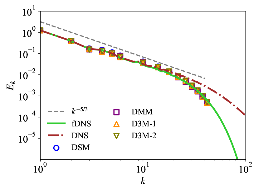
(d)

Figure 4: Velocity spectra of the a posteriori studies at a grid resolution of $N=128^{3}$ for different orders of discrete filters: (a) second-order, (b) fourth-order, (c) sixth-order, and (d) eighth-order.

Fig. 4 shows the predicted energy spectra of various models with different orders of discrete filters. When the filter order is 2, 4, 6, and 8, each model can predict the shape of the energy spectra well.

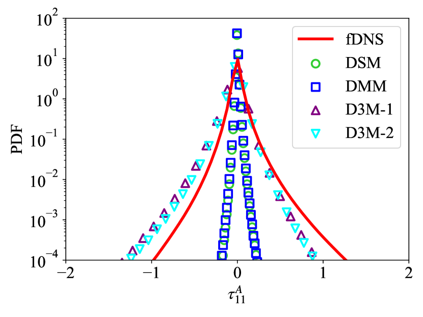
(a)

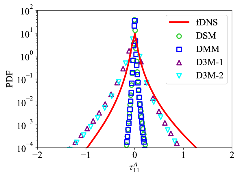
(b)

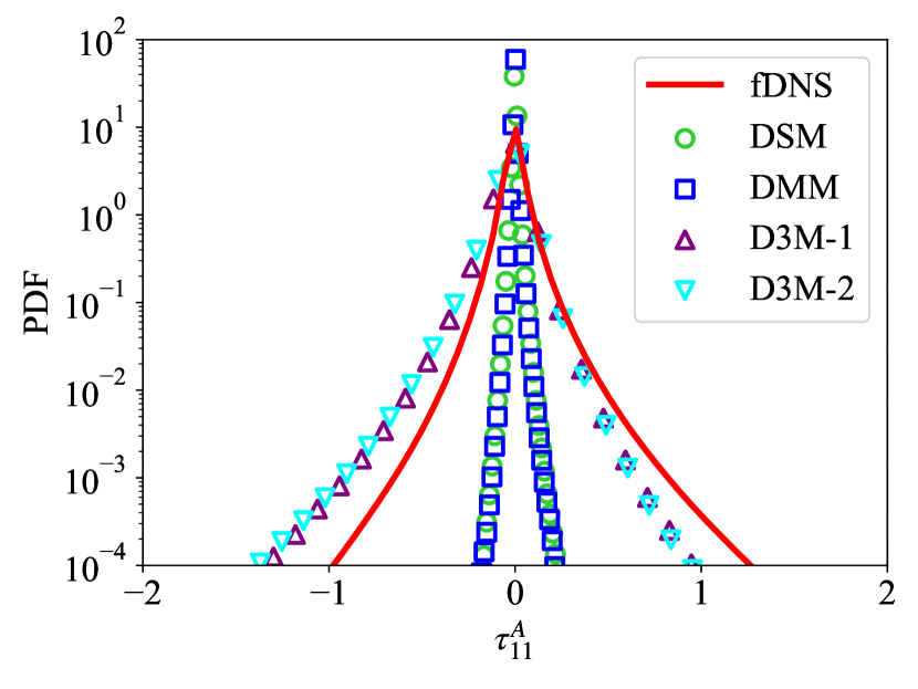
(c)

(d)

Figure 5: PDFs of the SFS stresses at a grid resolution of $N=128^{3}$ for different orders of discrete filters: (a) second-order, (b) fourth-order, (c) sixth-order, and (d) eighth-order.

The PDFs of SFS stresses are presented in Figs. 5 and 6, and the accuracy of SFS stresses predictions serves as a crucial metric for assessing the performance of SFS models. It is shown by Fig. 5 that PDFs of SFS normal stress, $\tau_{11}^{A}$, predicted by DSM and DMM are much narrower than the true values. The results predicted by D3M-1 and D3M-2 deviate slightly outward in the left half and inward in the right half.

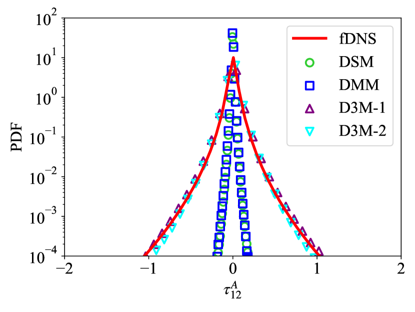
(a)

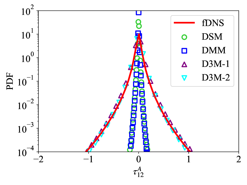
(b)

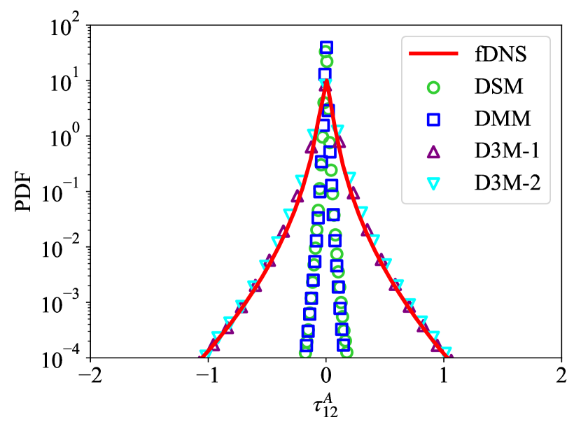
(c)

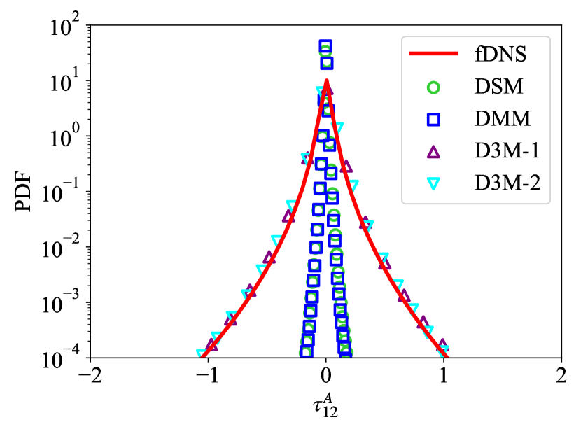
(d)

Figure 6: PDFs of the SFS stresses at a grid resolution of $N=128^{3}$ for different orders of discrete filters: (a) second-order, (b) fourth-order, (c) sixth-order, and (d) eighth-order.

The PDFs of SFS shear stress, $\tau_{12}^{A}$, are presented in Fig. 6. The results obtained by both D3M-1 and D3M-2 with different orders exhibit an excellent agreement with the fDNS data. The PDFs predicted by DSM and DMM are notably narrower compared with the fDNS data.

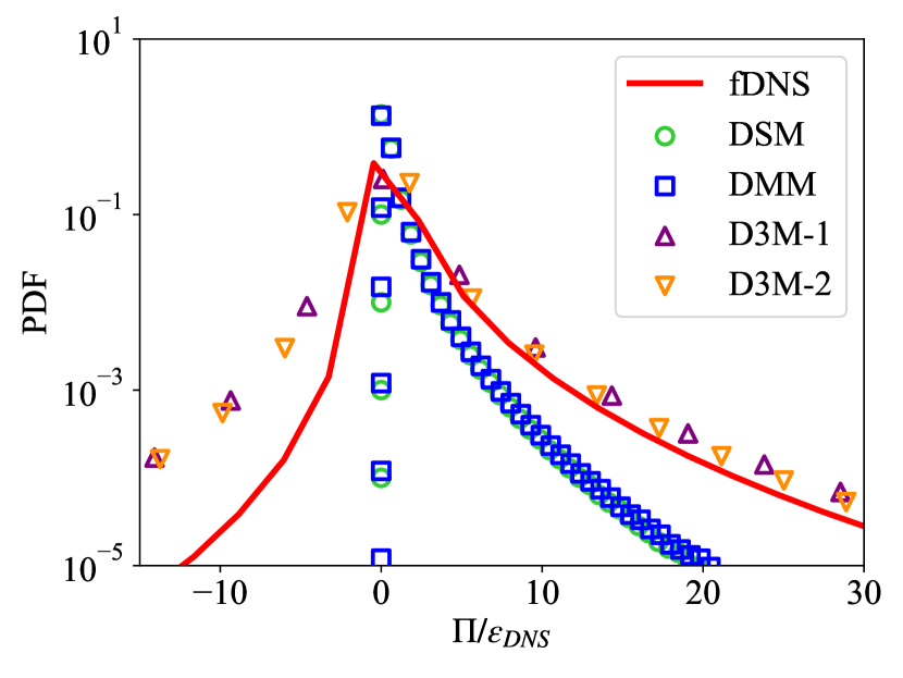
(a)

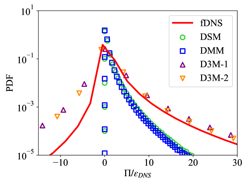
(b)

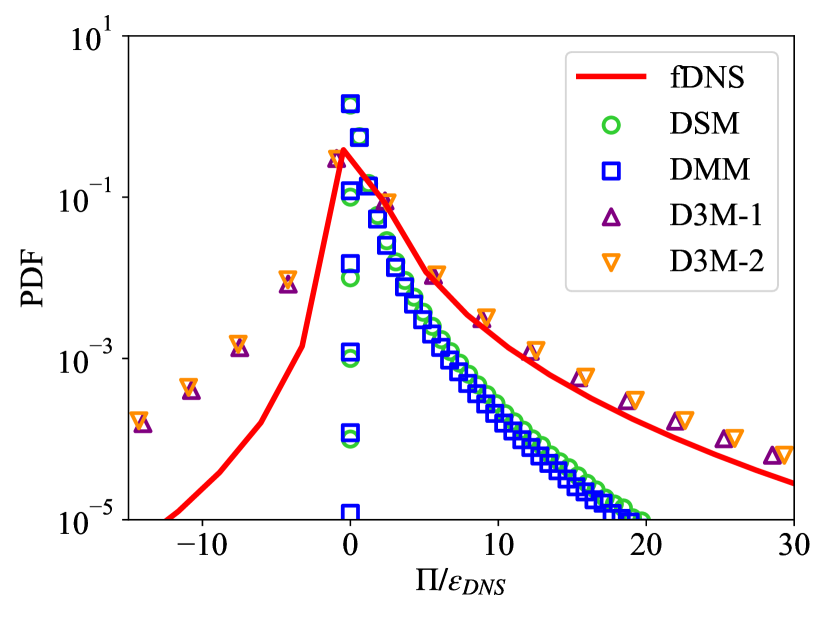
(c)

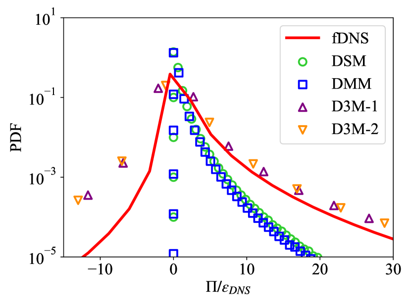
(d)

Figure 7: PDFs of the characteristic strain-rate at a grid resolution of $N=128^{3}$ for different orders of discrete filters: (a) second-order, (b) fourth-order, (c) sixth-order, and (d) eighth-order.

Fig. 7 shows the PDFs of SFS energy flux. The right half of PDFs predicted by DSM and DMM deviate significantly from the fDNS results. Additionally, the left half of DSM and DMM are basically concentrated around zero, indicating that these two models cannot predict the backscatter of SFS energy flux from small scales to large scales. For D3M-1 and D3M-2, their right halves are very close to the true values, while their left halves deviate due to the inaccurate prediction of SFS normal stress components.

(a)

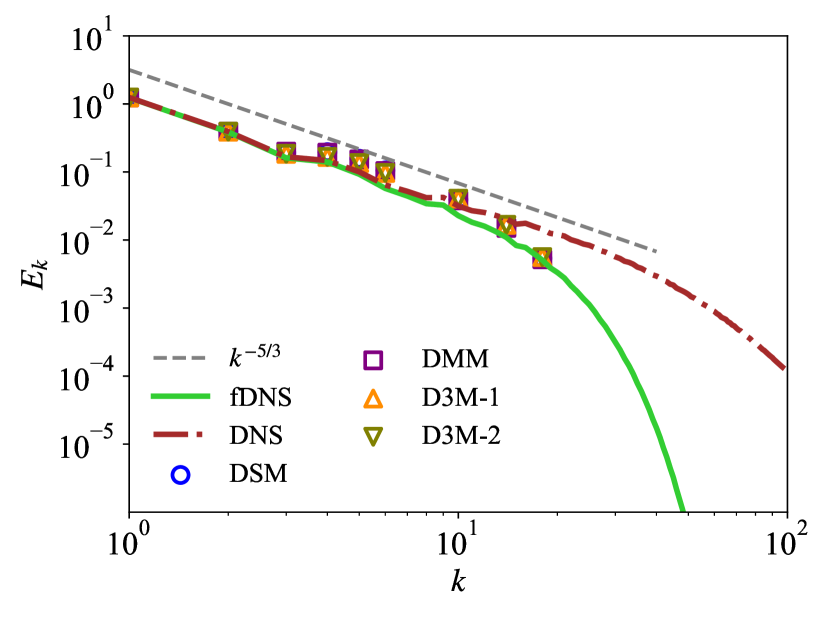
(b)

(c)

(d)

Figure 8: Velocity spectra of the a posteriori studies at a grid resolution of $N=64^{3}$ for different orders of discrete filters: (a) second-order, (b) fourth-order, (c) sixth-order, and (d) eighth-order.

Subsequently, we conducted tests to assess the generalization capability of discrete filters at different filter widths. These tests were performed on a grid of $N=64^{3}$, and the energy spectra are depicted in Fig. 8. Across filter orders ranging from the second to eighth, all models demonstrated excellent performance. The results indicate that when subjected to wider filter widths ($\bar{\Delta}=32h_{DNS}$), D3M-1 and D3M-2 can still exhibit strong predictive capabilities.

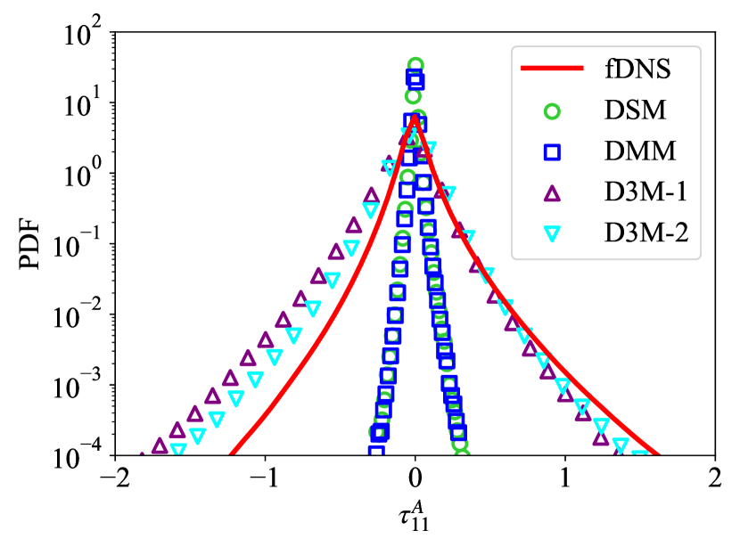
(a)

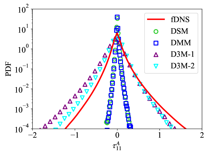
(b)

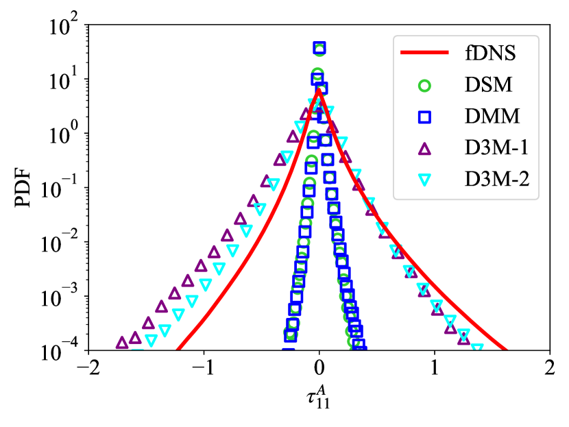
(c)

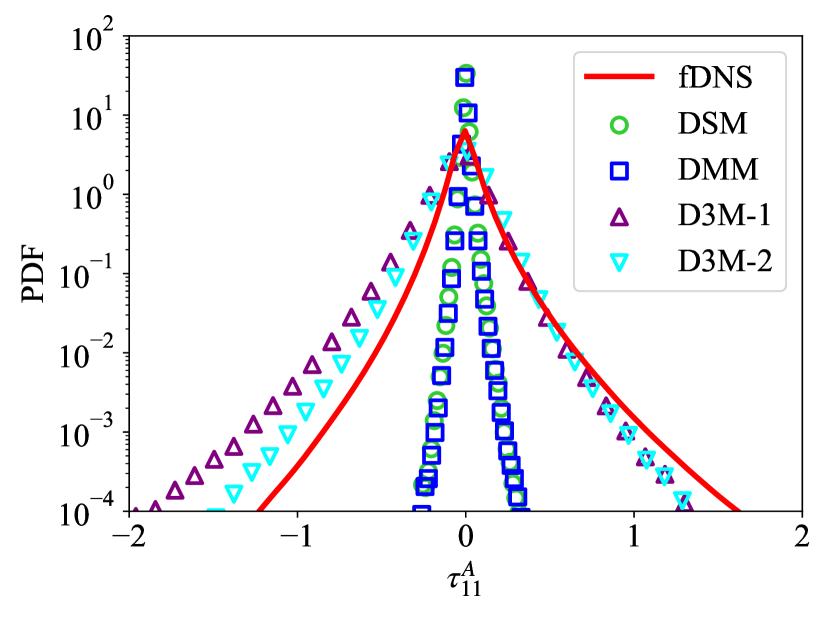
(d)

Figure 9: PDFs of the SFS stresses at a grid resolution of $N=64^{3}$ for different orders of discrete filters: (a) second-order, (b) fourth-order, (c) sixth-order, and (d) eighth-order.

Fig. 9 shows the predicted PDFs of SFS normal stresses, $\tau_{11}^{A}$, from various models using discrete filters of different orders. Compared to the results of fDNS, the predictions from DSM and DMM are too narrow and concentrate around zero. The right halves of the predictions from D3M-1 and D3M-2 are closer to that of fDNS, while the left halves deviate to the left, and D3M-2 deviates further to the left than D3M-1.

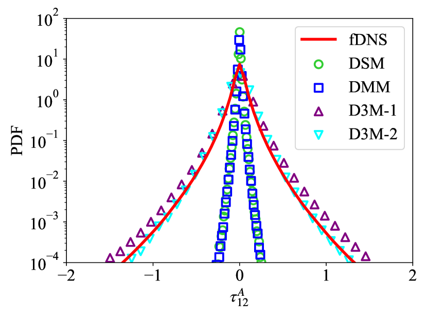
(a)

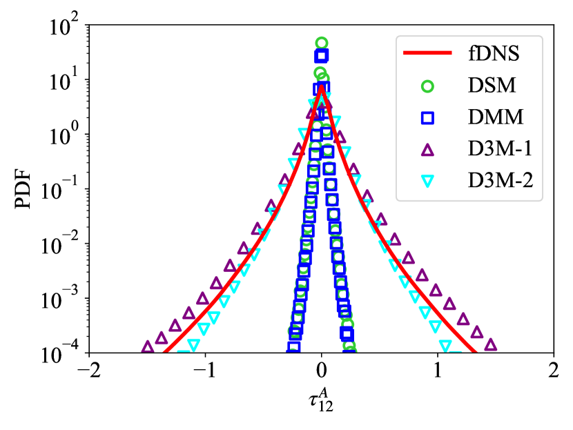
(b)

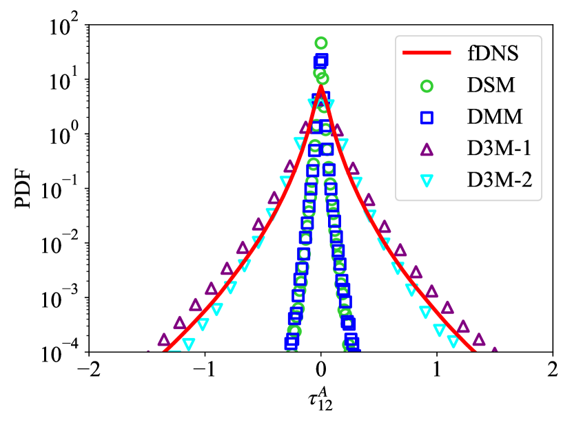
(c)

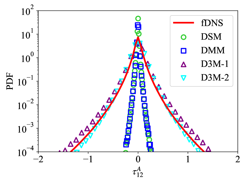
(d)

Figure 10: PDFs of the SFS stresses at a grid resolution of $N=64^{3}$ for different orders of discrete filters: (a) second-order, (b) fourth-order, (c) sixth-order, and (d) eighth-order.

Fig. 10 presents the predicted PDFs of SFS shear stresses, $\tau_{12}^{A}$, from various models using discrete filters of different orders. Compared to the fDNS results, the predictions from both DSM and DMM are still too narrow. D3M-1 exhibits an outward skewness in both its left and right halves relative to fDNS, while D3M-2 accurately predicts the distribution of the PDFs.

IV.2 Temporally evolving turbulent mixing layer (TML)

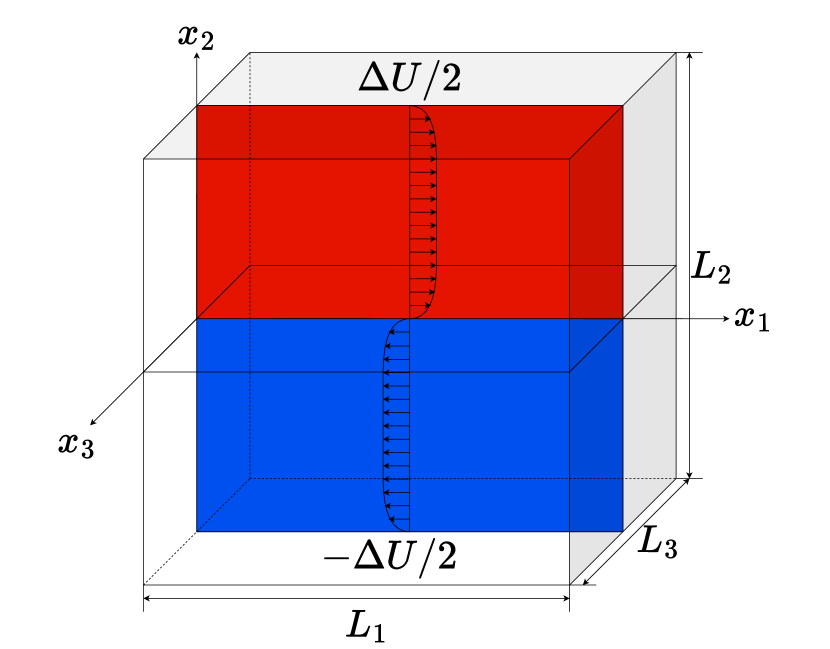
(a)

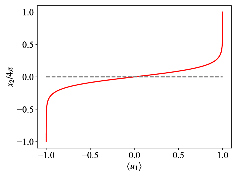
(b)

Figure 11: Diagram of the temporally evolving mixing layer with the mean velocity profile: (a) schematic of the mixing layer, and (b) mean streamwise velocity profile $\langle u_{1}\rangle$ along the normal ($x_{2}$) direction.

The TML involves both the unstable shear process of vortex shedding and the transition process from laminar flow to turbulence, making it a suitable candidate for studying the impact of non-uniform shear and mixing on SFS models. The governing equation for free-shear turbulence is also the Navier-Stokes equations [Eqs. 1 and 2] without the forcing term. Fig. 11 displays a schematic of the evolving turbulent mixing layer over time, with the initial condition being a hyperbolic tangent velocity profile.Sharan, Matheou, and Dimotakis (2019); Wang, Wang, and Chen (2022) The computational domain is a rectangular cuboid with dimensions $L_{1}\times L_{2}\times L_{3}=8\pi\times 8\pi\times 4\pi$, and the grid resolution is $N_{1}\times N_{2}\times N_{3}=512\times 512\times 256$. The symbols $x_{1}\in[-L_{1}/2,L_{1}/2]$, $x_{2}\in[-L_{2}/2,L_{2}/2]$, and $x_{3}\in[-L_{3}/2,L_{3}/2]$ represent the streamwise, transverse, and spanwise directions, respectively. The upper and lower layers of the shear layer have equal but opposite velocities, and $\Delta U=2$ is the velocity difference between them.

The momentum thickness represents the thickness of the turbulent region in the mixing layer, which is defined by

$$\delta_{\theta}=\int_{-L_{2}/4}^{L_{2}/4}\left[\frac{1}{4}-\left(\frac{\langle\bar{u}_{1}\rangle}{\Delta U}\right)^{2}\right]dx_{2},$$ (49)

where the $\langle\cdot\rangle$ represents spatial averaging in all uniform directions for the mixing layer, $x_{1}$ and $x_{3}$ directions. $\delta_{\theta}^{0}=0.08$ represents the initial momentum layer thickness, The initial transverse and spanwise velocities are set to zero. Since the initial average velocity field is periodic in all three directions, triply periodic boundary conditions are applied. The calculations use pseudospectral method and the 2/3 dealiasing rule. The time advancement uses the two-step Adam-Bashforth rule. To reduce the influence of the upper and lower boundaries on the intermediate mixing layer, numerical diffusion buffer layers are applied near the upper and lower boundaries of the computational domain.Wang, Wang, and Chen (2022); Klein, Sadiki, and Janicka (2003) The thickness of the buffer layer is set to $15\delta_{\theta}^{0}$, which is sufficient to provide buffering while having a negligible impact on the mixing layer calculations.

The spatially-correlated initial disturbances are achieved through digital filtering,Wang et al. (2022) with the width of the digital filter set to $\Delta_{d}=8h_{DNS}$, consistent with the filtering scale of the LES. The initial Reynolds stresses distribution of the digital filter is assumed to be a longitudinal distribution. The kinematic viscosity of the mixing layer is set to 0.0001. The corresponding Reynolds number defined based on the momentum thickness, $\mathrm{Re}_{\theta}$, has the expression as follows

$$\mathrm{Re}_{\theta}=\frac{\Delta U\delta_{\theta}}{\nu_{\infty}},$$ (50)

where $\nu_{\infty}$ is the viscosity coefficient of free flow.

To satisfy the periodic boundary conditions for the normal direction, the initial mean streamwise velocity is given by

$$\begin{gathered}\langle u_{1}\rangle=\frac{\Delta U}{2}\left[\tanh\left(\frac{x_{2}}{2\delta_{\theta}^{0}}\right)-\tanh\left(\frac{x_{2}+L_{2}/2}{2\delta_{\theta}^{0}}\right)-\tanh\left(\frac{x_{2}-L_{2}/2}{2\delta_{\theta}^{0}}\right)\right],\\ x\in\left[-\frac{L_{2}}{2}\leq x_{2}\leq\frac{L_{2}}{2}\right].\end{gathered}$$ (51)

The initial momentum thickness Reynolds number is set to 320, and the DNS parameters for the temporally evolving mixing layer are summarized in Table 8.

Table 8: Parameters for the DNS of the temporally evolving mixing layer.

$N_{1}\times N_{2}\times N_{3}$	$L_{1}\times L_{2}\times L_{3}$	$\nu_{\infty}$	$Re_{\theta}$	$\Delta_{\theta}^{0}$	$\Delta U$	$\Delta_{d}/h_{DNS}$	$h_{DNS}$	$\Delta t_{DNS}$
$512\times 512\times 256$	$8\pi\times 8\pi\times 4\pi$	$5\times{10^{-4}}$	4000	0.08	2	8	$\pi/64$	0.002

We have computed DNS for 800 time units ($t/\tau_{\theta}=800$), which is normalized by $\tau_{\theta}=\delta_{\theta}^{0}/\Delta U$.

(a)

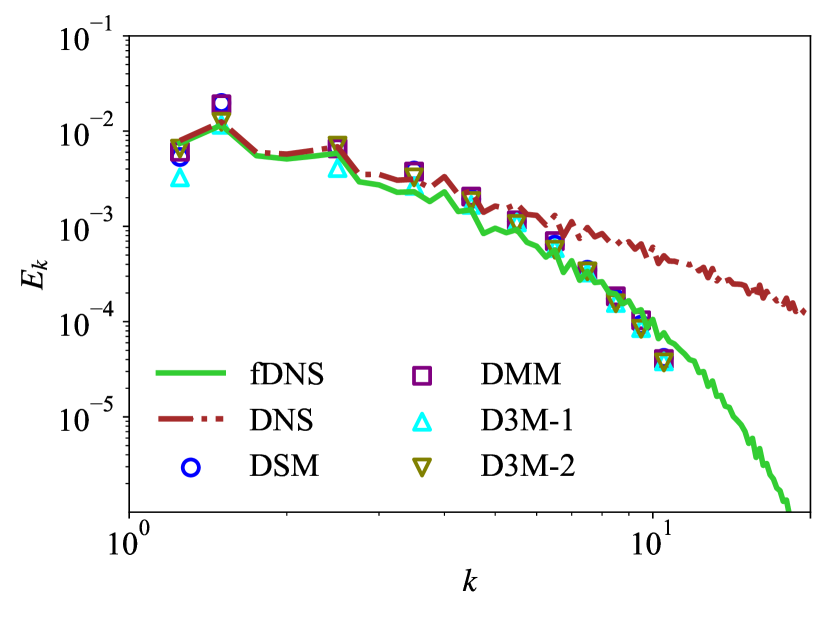
(b)

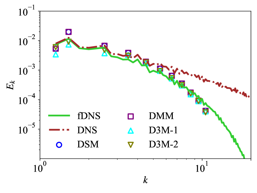
(c)

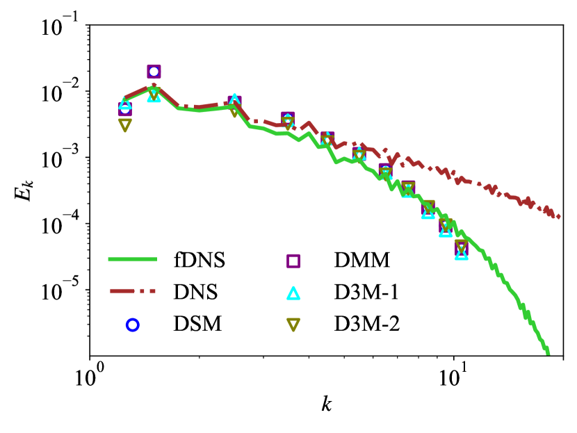
(d)

Figure 12: Velocity spectra for different SFS models in the a posteriori analysis of temporally evolving turbulent mixing layer with the filter scale $\bar{\Delta}=8h_{DNS}$ at $t/\tau_{\theta}\approx 500$ at a grid resolution of $N=128^{2}\times 64$ for different orders of discrete filters: (a) second-order, (b) fourth-order, (c) sixth-order, and (d) eighth-order.

The energy spectra of the temporally evolving mixing layer are shown in Fig. 12. For various orders of filters, when the wavenumber is less than 3, different models exhibit some differences. However, when the wavenumber is greater than 3, the energy spectra predicted by all models almost overlap.

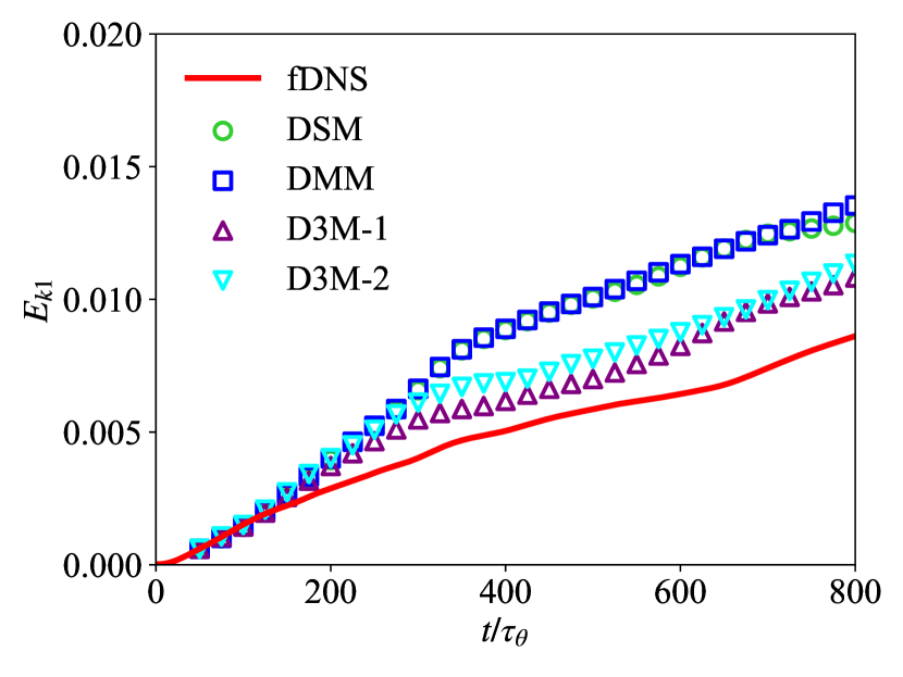
(a)

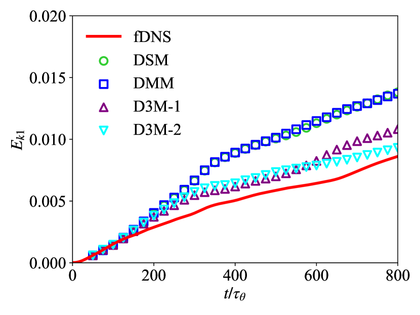
(b)

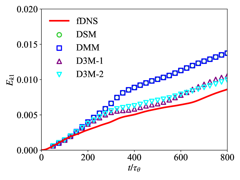
(c)

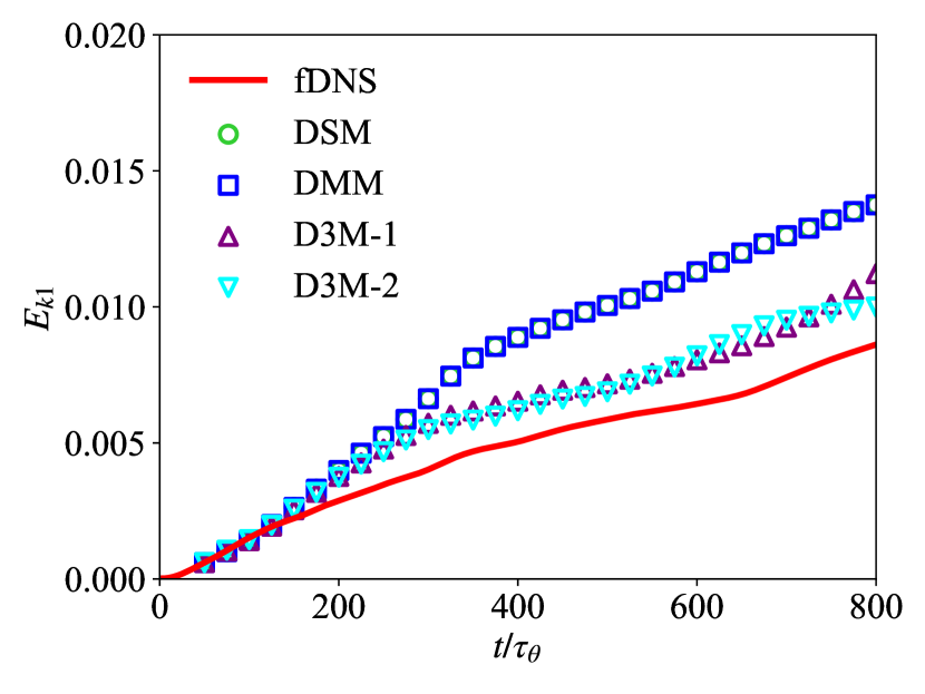
(d)

Figure 13: Streamwise turbulent kinetic energy for LES in the a posteriori analysis of temporally evolving turbulent mixing layer at a grid resolution of $N=128^{2}\times 64$ for different orders of discrete filters: (a) second-order, (b) fourth-order, (c) sixth-order, and (d) eighth-order.

Fig. 13 shows the temporal evolution of turbulent kinetic energy. For discrete filters of various orders, all models almost overlap with fDNS within the first 150 dimensionless time units, but deviate afterwards. DSM and DMM predict turbulent kinetic energy that is much higher than the actual fDNS turbulent kinetic energy. While D3M-1 and D3M-2 also experience some increase, the magnitude is much smaller than that of DSM and DMM, making them closer to the fDNS results.

(a)

(b)

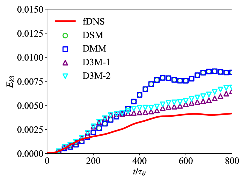
(c)

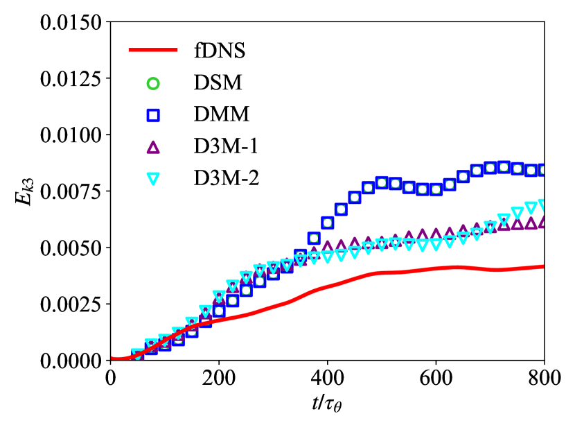
(d)

Figure 14: Spanwise turbulent kinetic energy for LES in the a posteriori analysis of temporally evolving turbulent mixing layer at a grid resolution of $N=128^{2}\times 64$ for different orders of discrete filters: (a) second-order, (b) fourth-order, (c) sixth-order, and (d) eighth-order.

Fig. 14 illustrates the temporal evolution of spanwise turbulent kinetic energy. Under different orders of discrete filters, the predictions from all models almost overlap with those of fDNS within the first 150 dimensionless time units. Afterward, the turbulent kinetic energy predicted by DSM and DMM is significantly higher than that of fDNS. In contrast, the predictions from D3M-1 and D3M-2 are much closer to the results of fDNS.

(a)

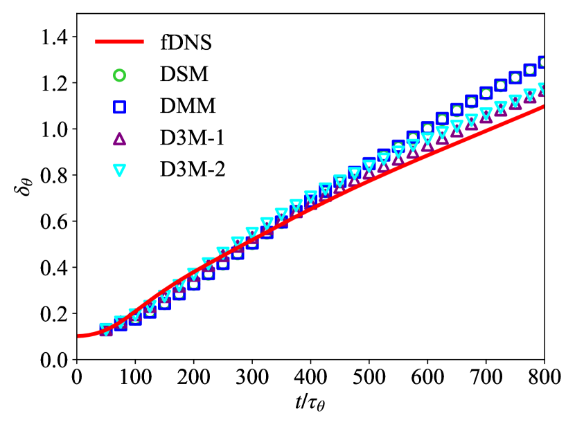
(b)

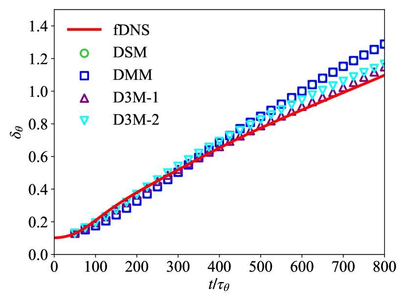
(c)

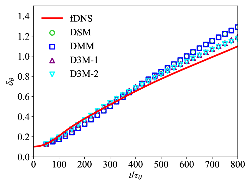
(d)

Figure 15: The evolution of the momentum thickness for LES in the a posteriori analysis of turbulent mixing layer with filter scale $\bar{\Delta}=8h_{DNS}$ at grid resolution of at $N=128^{2}\times 64$ for different orders of discrete filters: (a) second-order, (b) fourth-order, (c) sixth-order, and (d) eighth-order.

The variation of momentum layer thickness is shown in Fig. 15. When the dimensionless time is less than 200, the results of D3M-1 and D3M-2 basically overlap with those of fDNS, while the predictions of DSM and DMM are lower than fDNS. As the dimensionless time increases beyond 200, DSM and DMM gradually deviate from the fDNS results. Although D3M-1 and D3M-2 also show some deviation, the degree is smaller than that of DSM and DMM, especially for D3M-1, which is very close to the fDNS results under various filter orders.

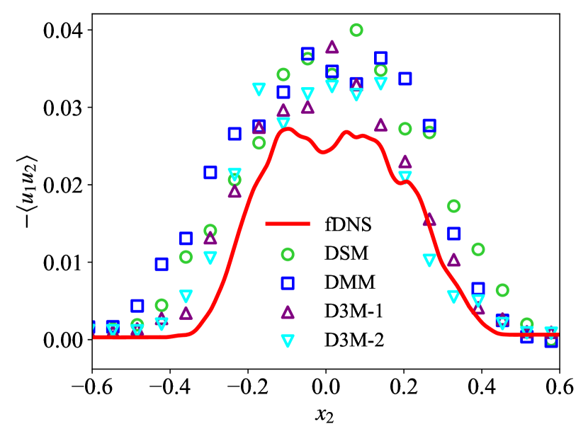
(a)

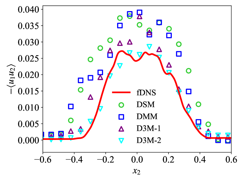
(b)

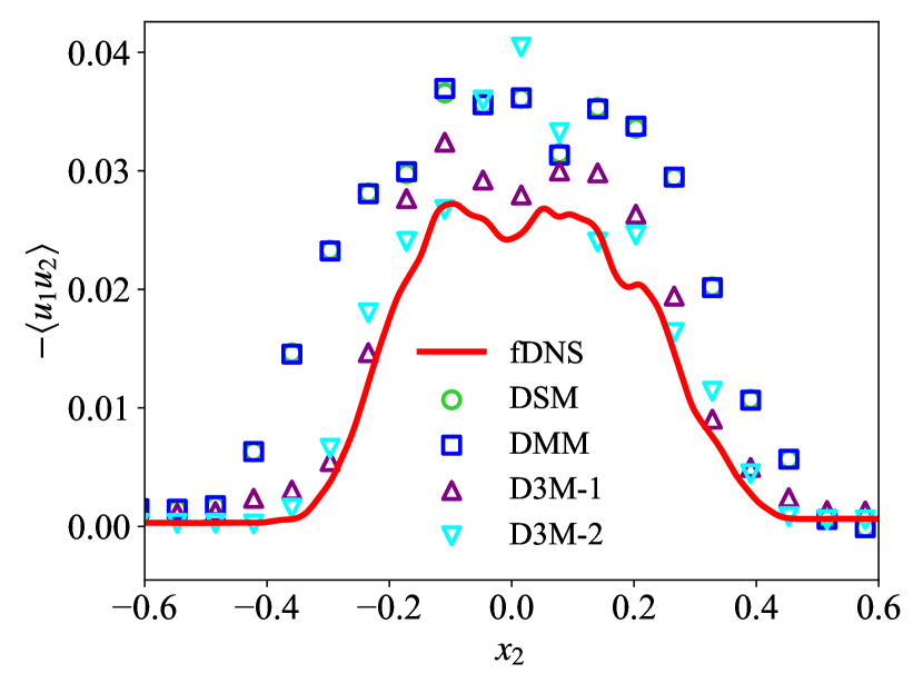
(c)

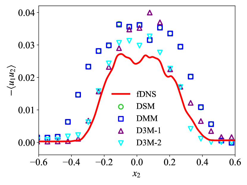
(d)

Figure 16: Transient profile (at $t/\tau_{\theta}\approx 500$) of the resolved Reynolds stresses $\bar{R}_{12}=\langle\bar{u}_{1}^{\prime}\bar{u}_{2}^{\prime}\rangle$ along the cross-stream direction for LES in the a posteriori analysis of temporally evolving turbulent mixing layer with filter scale $\bar{\Delta}=8h_{DNS}$ at a grid resolution of at $N=128^{2}\times 64$ for different orders of discrete filters: (a) second-order, (b) fourth-order, (c) sixth-order, and (d) eighth-order.

Fig. 16 presents the instantaneous distribution of Reynolds stresses. When the order of the discrete filter is 2, DSM and DMM deviate significantly from fDNS. The right halves of D3M-1 and D3M-2 are relatively close to the results of fDNS, while the left halves show some deviation. As the order increases to 4, DSM and DMM still exhibit large deviations from fDNS, while D3M-2 aligns well with fDNS. D3M-1 performs slightly worse than D3M-2, showing some deviation at the top and left halves. When the orders are 6 and 8, DSM and DMM differ significantly from fDNS. However, D3M-1 and D3M-2 predict well except for some deviation at the top.

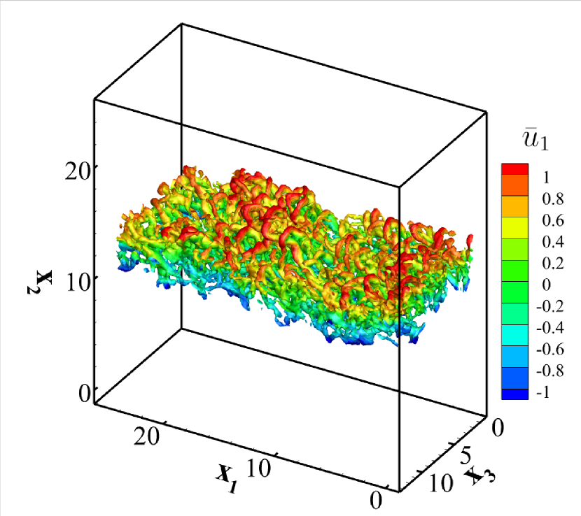
(a) fDNS

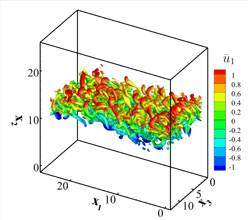
(b) DSM

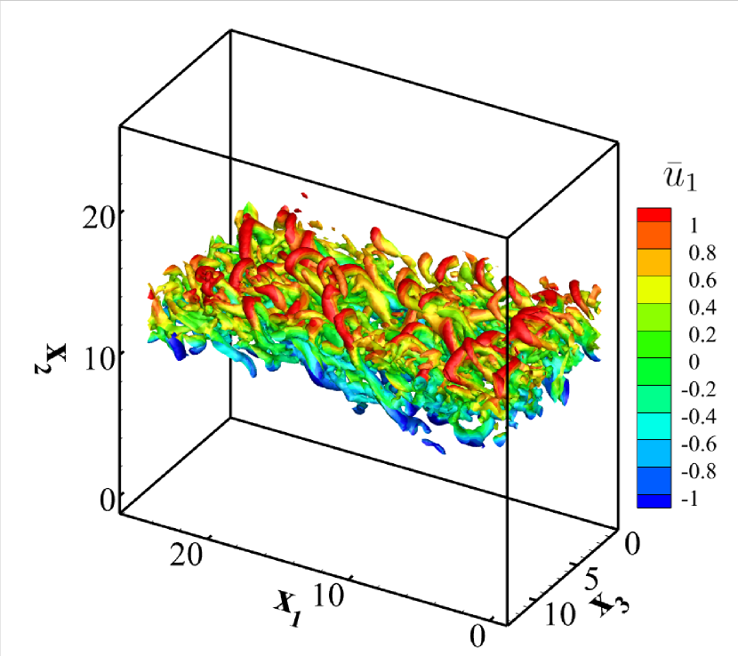
(c) DMM

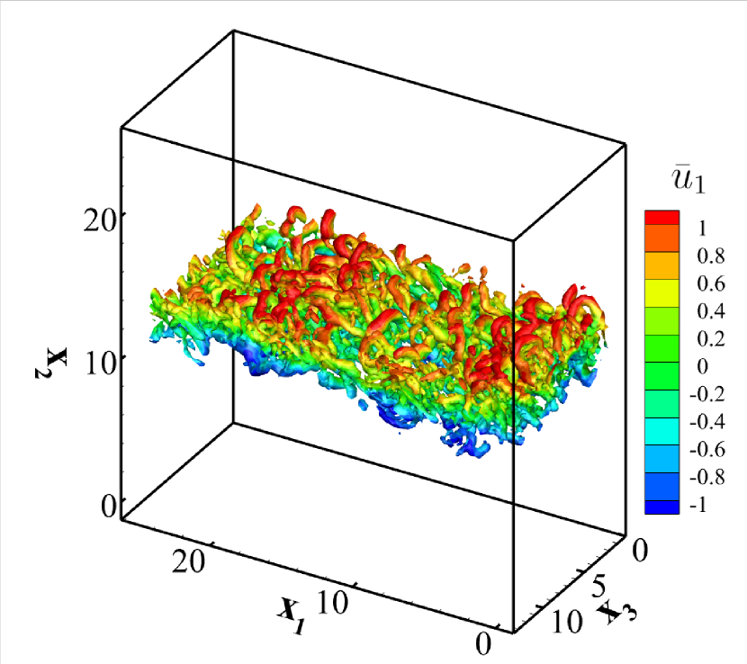
(d) D3M-1

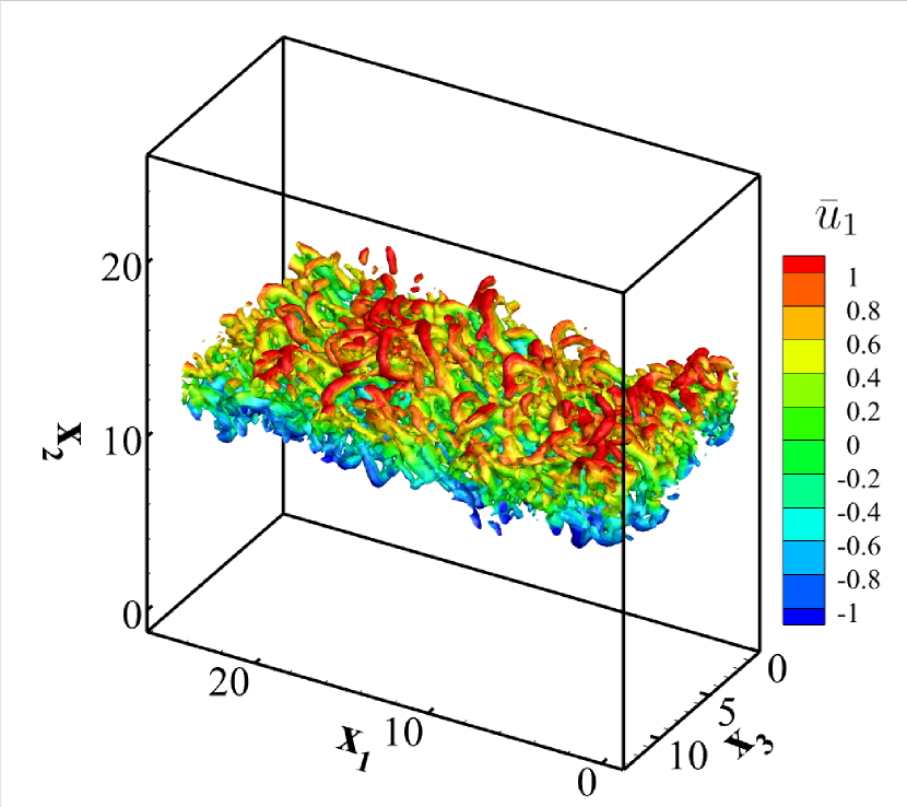
(e) D3M-2

Figure 17: Transient iso-surfaces (at $t/\tau_{\theta}\approx 500$) of the Q-criterion at $\mathrm{Q}=0.2$, colored by the streamwise velocity in the a posteriori analysis of temporally evolving turbulent mixing layer with filter scale $\bar{\Delta}=8h_{DNS}$ at grid resolution of at $N=128^{2}\times 64$ with the fourth-order of discrete filter: (a) fDNS, (b) DSM, (c) DMM, (d) D3M-1, and (e) D3M-2.

Fig. 17 shows the instantaneous iso-surfaces of the Q criterion. The Q criterion is an important quantity used for visualizing vortex structures, and its definition is

$$Q=\frac{1}{2}\left(\bar{\Omega}_{ij}\bar{\Omega}_{ij}-\bar{S}_{ij}\bar{S}_{ij}\right),$$ (52)

where $\bar{\Omega}_{ij}=\frac{1}{2}(\partial{\bar{u}_{i}}/\partial{\bar{x}_{j}}-\partial{\bar{u}_{j}}/\partial{\bar{x}_{i}})$ is the rotation-rate tensor. It can be observed that in fDNS, there are abundant structures of various scales, and the vortex structures at the top are concentrated in two distinct regions. However, the structures predicted by DSM and DMM are significantly larger, and the boundary between the two regions at the top is not clear. On the other hand, the structures predicted by D3M-1 and D3M-2 are closer in scale to those of fDNS, and the vortex structures at the top can be clearly divided into two regions.

V CONCLUSION

In this study, we have developed discrete direct deconvolution models D3M-1 and D3M-2, and compared them with the traditional DSM and DMM. In the a priori study, the correlation coefficients of D3M-1 and D3M-2 are more than 94%, and the relative errors are less than 40%. As the order of the discrete filter increases, the correlation coefficients of the model tend to increase, while the relative errors decrease.

In the a posteriori study, we select HIT and TML to investigate the effects of different models. In the HIT cases, D3M-1 and D3M-2 can effectively predict the shape of the velocity spectra, as well as the PDFs of SFS stresses and SFS energy flux. These models exhibit generalization capabilities across different filter widths. Furthermore, D3M-1 and D3M-2 accurately predict instantaneous flow structures.

In the TML cases, D3M-1 and D3M-2 demonstrate advantages over traditional DSM and DMM in terms of velocity spectra, turbulent kinetic energy, momentum layer thickness, and Reynolds stresses. When predicting spatially coherent structures in the flow field, the results of D3M-1 and D3M-2 are closer to the benchmark values of fDNS, outperforming traditional models. These results indicate that the D3M-1 and D3M-2 have a considerable potential for high-fidelity LES.

DATA AVAILABILITY

The data that support the findings of this study are available from the corresponding author upon reasonable request.

Appendix A THE DISCRETE GAUSSIAN FILTER

A.1 D3M-1

A.1.1 Convolution

In the physical space, the Gaussian filter is

$$G(r)=\left(\frac{6}{\pi\bar{\Delta}^{2}}\right)^{\frac{1}{2}}\exp\left(-\frac{6r^{2}}{\bar{\Delta}^{2}}\right).$$ (53)

The filtered quantity $\bar{\phi}$ is defined by

$$\bar{\phi}(x)=\int_{-\infty}^{+\infty}G(x-y)\phi(y)dy.$$ (54)

Starting from the Taylor’s expansion, we have

$$\phi(y)=\phi(x)+\sum_{l=1}^{\infty}\frac{(y-x)^{l}}{l!}\frac{\partial^{l}\phi(x)}{\partial\xi^{l}}.$$ (55)

Insert Eq. 55 into Eq. 54, we have

$$\bar{\phi}(x)=\phi(x)+\sum_{l=1}^{\infty}\frac{M_{l}}{l!}\frac{\partial^{l}\phi(x)}{\partial x^{l}}.$$ (56)

Here, $M_{l}$ is the moment of order $l$ of the kernel $G$, namely,

$$M_{l}=\int_{-\infty}^{+\infty}G(r)r^{l}dr=\int_{-\infty}^{+\infty}\left(\frac{6}{\pi\bar{\Delta}^{2}}\right)^{\frac{1}{2}}\exp\left(-\frac{6r^{2}}{\bar{\Delta}^{2}}\right)r^{l}dr.$$ (57)

Since

$$\int_{-\infty}^{+\infty}r^{2n}e^{-ar^{2}}dr=\sqrt{\frac{\pi}{a}}\frac{(2n-1)!!}{(2a)^{n}},$$ (58)

and $\exp\left(-\frac{6r^{2}}{\bar{\Delta}^{2}}\right)$ is an even function, we have,Sagaut (2006)

$$\begin{gathered}M_{1}=0,\ M_{2}=\frac{\bar{\Delta}^{2}}{12},\ M_{3}=0,\ M_{4}=\frac{\bar{\Delta}^{4}}{48},\\ M_{5}=0,\ M_{6}=\frac{5\bar{\Delta}^{6}}{576},\ M_{7}=0,\ \mathrm{and}\ M_{8}=\frac{35\bar{\Delta}^{8}}{6912}.\end{gathered}$$ (59)

Namely,Sagaut and Grohens (1999); Nikolaou, Vervisch, and Domingo (2023)

$$\bar{\phi}(x)=\phi(x)+\frac{\bar{\Delta}^{2}}{24}\frac{\partial^{2}\phi}{\partial x^{2}}+\frac{\bar{\Delta}^{4}}{1152}\frac{\partial^{4}\phi}{\partial x^{4}}+\frac{\bar{\Delta}^{6}}{82944}\frac{\partial^{6}\phi}{\partial x^{6}}+\frac{\bar{\Delta}^{8}}{7962624}\frac{\partial^{8}\phi}{\partial x^{8}}+O\left(\bar{\Delta}^{10}\right).$$ (60)

Accordingly,

$$G=1+\frac{\bar{\Delta}^{2}}{24}\frac{\partial^{2}}{\partial x^{2}}+\frac{\bar{\Delta}^{4}}{1152}\frac{\partial^{4}}{\partial x^{4}}+\frac{\bar{\Delta}^{6}}{82944}\frac{\partial^{6}}{\partial x^{6}}+\frac{\bar{\Delta}^{8}}{7962624}\frac{\partial^{8}}{\partial x^{8}}+O\left(\bar{\Delta}^{10}\right).$$ (61)

Assume thatSagaut and Grohens (1999); Nikolaou, Vervisch, and Domingo (2023)

$$\bar{\phi}_{j}=\sum_{m=-\frac{N}{2}}^{\frac{N}{2}}a_{m}\phi_{j+m},$$ (62)

where the subscript $j$ denotes the index of the grid point, not the component in the $j$th-direction. $N$ represents the order of the discrete filter. According to the Taylor’s expansion, we have

$$\phi_{j+m}=\phi_{j}+\left[\sum_{l=1}^{N}\left(\frac{m\bar{\Delta}}{\alpha}\right)^{l}\frac{1}{l!}\frac{\partial^{l}\phi_{j}}{\partial x^{l}}\right]+O\left(\bar{\Delta}^{N+1}\right).$$ (63)

For $N=8$,

$$\phi_{j+m}= \phi_{j}+\frac{m\bar{\Delta}}{\alpha}\frac{\partial\phi_{j}}{\partial x}+\frac{1}{2}\frac{m^{2}\bar{\Delta}^{2}}{\alpha^{2}}\frac{\partial^{2}\phi_{j}}{\partial x^{2}}+\frac{1}{6}\frac{m^{3}\bar{\Delta}^{3}}{\alpha^{3}}\frac{\partial^{3}\phi_{j}}{\partial x^{3}}$$ (64)

$$+\frac{1}{24}\frac{m^{4}\bar{\Delta}^{4}}{\alpha^{4}}\frac{\partial^{4}\phi_{j}}{\partial x^{4}}+\frac{1}{120}\frac{m^{5}\bar{\Delta}^{5}}{\alpha^{5}}\frac{\partial^{5}\phi_{j}}{\partial x^{5}}+\frac{1}{720}\frac{m^{6}\bar{\Delta}^{6}}{\alpha^{6}}\frac{\partial^{6}\phi_{j}}{\partial x^{6}}$$

$$+\frac{1}{5040}\frac{m^{7}\bar{\Delta}^{7}}{\alpha^{7}}\frac{\partial^{7}\phi_{j}}{\partial x^{7}}+\frac{1}{40320}\frac{m^{8}\bar{\Delta}^{8}}{\alpha^{8}}\frac{\partial^{8}\phi_{j}}{\partial x^{8}}+O\left(\bar{\Delta}^{9}\right).$$

Substitute Eq. 64 into Eq. 62, we obtain

$$\begin{gathered}\bar{\phi}_{j}=\left(\sum_{m=-\frac{N}{2}}^{\frac{N}{2}}a_{m}\right)\phi_{j}+\left(\sum_{m=-\frac{N}{2}}^{\frac{N}{2}}ma_{m}\right)\frac{\bar{\Delta}}{\alpha}\frac{\partial\phi_{j}}{\partial x}+\frac{1}{2}\left(\sum_{m=-\frac{N}{2}}^{\frac{N}{2}}m^{2}a_{m}\right)\frac{\bar{\Delta}^{2}}{\alpha^{2}}\frac{\partial^{2}\phi_{j}}{\partial x^{2}}\\ +\frac{1}{6}\left(\sum_{m=-\frac{N}{2}}^{\frac{N}{2}}m^{3}a_{m}\right)\frac{\bar{\Delta}^{3}}{\alpha^{3}}\frac{\partial^{3}\phi_{j}}{\partial x^{3}}+\frac{1}{24}\left(\sum_{m=-\frac{N}{2}}^{\frac{N}{2}}m^{4}a_{m}\right)\frac{\bar{\Delta}^{4}}{\alpha^{4}}\frac{\partial^{4}\phi_{j}}{\partial x^{4}}\\ +\frac{1}{120}\left(\sum_{m=-\frac{N}{2}}^{\frac{N}{2}}m^{5}a_{m})\right)\frac{\bar{\Delta}^{5}}{\alpha^{5}}\frac{\partial^{5}\phi_{j}}{\partial x^{5}}+\frac{1}{720}\left(\sum_{m=-\frac{N}{2}}^{\frac{N}{2}}m^{6}a_{m}\right)\frac{\bar{\Delta}^{6}}{\alpha^{6}}\frac{\partial^{6}\phi_{j}}{\partial x^{6}}\\ +\frac{1}{5040}\left(\sum_{m=-\frac{N}{2}}^{\frac{N}{2}}m^{7}a_{m}\right)\frac{\bar{\Delta}^{7}}{\alpha^{7}}\frac{\partial^{7}\phi_{j}}{\partial x^{7}}+\frac{1}{40320}\left(\sum_{m=-\frac{N}{2}}^{\frac{N}{2}}m^{8}a_{m}\right)\frac{\bar{\Delta}^{8}}{\alpha^{8}}\frac{\partial^{8}\phi_{j}}{\partial x^{8}}.\end{gathered}$$ (65)

Truncate Eq. 60 and Eq. 65 to the specific order, we obtain a system of equations that the coefficients satisfy. For the second-order discrete filter, the coefficients satisfy the following equations.

$$\begin{gathered}a_{-1}+a_{0}+a_{1}=1,\\ (-a_{-1}+a_{1})\frac{\bar{\Delta}}{\epsilon}=0,\\ \frac{1}{2}(a_{-1}+a_{1})\frac{\bar{\Delta}^{2}}{\epsilon^{2}}=\frac{\bar{\Delta}^{2}}{24}.\end{gathered}$$ (66)

For the fourth-order discrete filter, the coefficients satisfy the following equations.

$$a_{-2}+a_{-1}+a_{0}+a_{1}+a_{2} =1,$$ (67)

$$(-2a_{-2}-a_{-1}+a_{1}+2a_{2})\frac{\bar{\Delta}}{\epsilon} =0,$$

$$\frac{1}{2}(4a_{-2}+a_{-1}+a_{1}+4a_{2})\frac{\bar{\Delta}^{2}}{\epsilon^{2}} =\frac{\bar{\Delta}^{2}}{24},$$

$$\frac{1}{6}(-8a_{-2}-a_{-1}+a_{1}+8a_{2})\frac{\bar{\Delta}^{3}}{\epsilon^{3}} =0,$$

$$\frac{1}{24}(16a_{-2}+a_{-1}+a_{1}+16a_{2})\frac{\bar{\Delta}^{4}}{\epsilon^{4}} =\frac{\bar{\Delta}^{4}}{1152}.$$

For the sixth-order discrete filter, the coefficients satisfy the following equations.

$$a_{-3}+a_{-2}+a_{-1}+a_{0}+a_{1}+a_{2}+a_{3} =1,$$ (68)

$$(-3a_{-3}-2a_{-2}-a_{-1}+a_{1}+2a_{2}+3a_{3})\frac{\bar{\Delta}}{\epsilon} =0,$$

$$\frac{1}{2}(9a_{-3}+4a_{-2}+a_{-1}+a_{1}+4a_{2}+9a_{3})\frac{\bar{\Delta}^{2}}{\epsilon^{2}} =\frac{\bar{\Delta}^{2}}{24},$$

$$\frac{1}{6}(-27a_{-3}-8a_{-2}-a_{-1}+a_{1}+8a_{2}+27a_{3})\frac{\bar{\Delta}^{3}}{\epsilon^{3}} =0,$$

$$\frac{1}{24}(81a_{-3}+16a_{-2}+a_{-1}+a_{1}+16a_{2}+81a_{3})\frac{\bar{\Delta}^{4}}{\epsilon^{4}} =\frac{\bar{\Delta}^{4}}{1152},$$

$$\frac{1}{120}(-243a_{-3}-32a_{-2}-a_{-1}+a_{1}+32a_{2}+249a_{3})\frac{\bar{\Delta}^{5}}{\epsilon^{5}} =0,$$

$$\frac{1}{720}(729a_{-3}+64a_{-2}+a_{-1}+a_{1}+64a_{2}+729a_{3})\frac{\bar{\Delta}^{6}}{\epsilon^{6}} =\frac{\bar{\Delta}^{6}}{82944}.$$

For the eighth-order discrete filter, the coefficients satisfy the following equations.

$$a_{-4}+a_{-3}+a_{-2}+a_{-1}+a_{0}+a_{1}+a_{2}+a_{3}+a_{4} =1,$$ (69)

$$(-4a_{-4}-3a_{-3}-2a_{-2}-a_{-1}+a_{1}+2a_{2}+3a_{3}+4a_{4})\frac{\bar{\Delta}}{\epsilon} =0,$$

$$\frac{1}{2}(16a_{-4}+9a_{-3}+4a_{-2}+a_{-1}+a_{1}+4a_{2}+9a_{3}+16a_{4})\frac{\bar{\Delta}^{2}}{\epsilon^{2}} =\frac{\bar{\Delta}^{2}}{24},$$

$$\frac{1}{6}(-64a_{-4}-27a_{-3}-8a_{-2}-a_{-1}+a_{1}+8a_{2}+27a_{3}+64a_{4})\frac{\bar{\Delta}^{3}}{\epsilon^{3}} =0,$$

$$\frac{1}{24}(256a_{-4}+81a_{-3}+16a_{-2}+a_{-1}+a_{1}+16a_{2}+81a_{3}+256a_{4})\frac{\bar{\Delta}^{4}}{\epsilon^{4}} =\frac{\bar{\Delta}^{4}}{1152},$$

$$\frac{1}{120}(-1024a_{-4}-243a_{-3}-32a_{-2}-a_{-1}+a_{1}+32a_{2}+249a_{3}+1024a_{4})\frac{\bar{\Delta}^{5}}{\epsilon^{5}} =0,$$

$$\frac{1}{720}(4096a_{-4}+729a_{-3}+64a_{-2}+a_{-1}+a_{1}+64a_{2}+729a_{3}+4096a_{4})\frac{\bar{\Delta}^{6}}{\epsilon^{6}} =\frac{\bar{\Delta}^{6}}{82944},$$

$$\frac{1}{5040}(-16384a_{-4}-2187a_{-3}-128a_{-2}-a_{-1}+a_{1}+128a_{2}+2187a_{3}+16384a_{4})\frac{\bar{\Delta}^{7}}{\epsilon^{7}} =0,$$

$$\frac{1}{40320}(65536a_{-4}+6561a_{-3}+256a_{-2}+a_{-1}+a_{1}+256a_{2}+6561a_{3}+65536a_{4})\frac{\bar{\Delta}^{8}}{\epsilon^{8}} =\frac{\bar{\Delta}^{8}}{7962624}.$$

By solving Eqs. 66, 67, 68 and 69, we obtain the coefficients for different orders as shown in Table 9.Nikolaou, Vervisch, and Domingo (2023) Here, $\alpha=\bar{\Delta}_{i}/h_{i}^{LES}$ is the FGR, where $\bar{\Delta}_{i}$ is the filtering width in the i-th direction, and $h_{i}^{LES}$ is the grid spacing of the LES.

Table 9: Coefficients of the discrete filters at different orders for both D3M-1 and D3M-2.

coefficients	2nd order	4th order	6th order	8th order
$a_{0}$	$\frac{12-\alpha^{2}}{12}$	$\frac{\alpha^{4}-20\alpha^{2}+192}{192}$	$\frac{-5\alpha^{6}+168\alpha^{4}-2352\alpha^{2}+20736}{20736}$	$\frac{35\alpha^{8}-1800\alpha^{6}+39312\alpha^{4}-472320\alpha^{2}+3981312}{3981312}$
$a_{1}=a_{-1}$	$\frac{\alpha^{2}}{24}$	$\frac{16\alpha^{2}-\alpha^{4}}{288}$	$\frac{5\alpha^{6}-156\alpha^{4}+1728\alpha^{2}}{27648}$	$\frac{-35\alpha^{8}+1740\alpha^{6}-35136\alpha^{4}+331776\alpha^{2}}{4976640}$
$a_{2}=a_{-2}$		$\frac{\alpha^{4}-4\alpha^{2}}{1152}$	$\frac{-5\alpha^{6}+120\alpha^{4}-432\alpha^{2}}{69120}$	$\frac{35\alpha^{8}-1560\alpha^{6}+24336\alpha^{4}-82944\alpha^{2}}{9953280}$
$a_{3}=a_{-3}$			$\frac{5\alpha^{6}-60\alpha^{4}+192\alpha^{2}}{414720}$	$\frac{-35\alpha^{8}+1260\alpha^{6}-12096\alpha^{4}+36864\alpha^{2}}{34836480}$
$a_{4}=a_{-4}$				$\frac{35\alpha^{8}-840\alpha^{6}+7056\alpha^{4}-20736\alpha^{2}}{278691840}$

A.1.2 Deconvolution

For a general filter function, $G(r)$, its transfer function isPope (2000)

$$\hat{G}(\kappa)\equiv\int_{-\infty}^{\infty}e^{-\underline{i}\kappa r}G(r)dr.$$ (70)

The discrete form of Eq. 70 isSagaut and Grohens (1999); Nikolaou, Vervisch, and Domingo (2023)

$$\hat{G}(\kappa) =\sum_{m=-N/2}^{N/2}e^{-\underline{i}\kappa r_{m}}a_{m},$$ (71)

$$=a_{0}+\sum_{m=1}^{N/2}2\cos(m\kappa\bar{\Delta})a_{m}.$$

Thus, the inverse of Eq. 71 is

$$\hat{G}^{-1}(\kappa)=\frac{1}{a_{0}+\sum_{m=1}^{N/2}2\cos(m\kappa\bar{\Delta})a_{m}}.$$ (72)

A.2 D3M-2

Assume the inverse of the filter $G$ exists, then

$$\phi^{*}=G^{-1}\otimes\bar{\phi}.$$ (73)

Since

$$G^{-1}=[I-(I-G)]^{-1},$$ (74)

and $(1-x)^{-1}$ can be expanded asSpivak (2006)

$$\frac{1}{1-x}=1+x+x^{2}+\cdots+x^{n}+\cdots,\quad(-1<x<1),$$ (75)

we obtain

$$G^{-1}=\sum_{p=0}^{\infty}(I-G)^{p}.$$ (76)

Let $p=4$, then

$$G^{-1} =1+(1-G)+(1-G)^{2}+(1-G)^{3}+(1-G)^{4},$$ (77)

$$=5-10G+10G^{2}-5G^{3}+G^{4}.$$

Substitute the Gaussian filter Eqs. 77 and 61 back to Eq. 73.

$$\phi^{*} =G^{-1}\otimes\bar{\phi},$$ (78)

$$=\left(5-10G+10G^{2}-5G^{3}+G^{4}\right)\otimes\bar{\phi},$$

$$=\left[1-\frac{\bar{\Delta}^{2}}{24}\frac{\partial^{2}}{\partial x^{2}}+\frac{\bar{\Delta}^{4}}{1152}\frac{\partial^{4}}{\partial x^{4}}-\frac{\bar{\Delta}^{6}}{82944}\frac{\partial^{6}}{\partial x^{6}}+\frac{\bar{\Delta}^{8}}{7962624}\frac{\partial^{8}}{\partial x^{8}}+O\left(\bar{\Delta}^{10}\right)\right]\bar{\phi}.$$

Assume thatNikolaou, Vervisch, and Domingo (2023)

$$\phi_{j}^{*}=\sum_{m=-\frac{N}{2}}^{\frac{N}{2}}a_{m}\bar{\phi}_{j+m},$$ (79)

where the subscript $j$ denotes the index of the grid point, not the component in the $j$th-direction. $N$ represents the order of the discrete filter. Likewise, following the similar procedures in deriving Eq. 65, we can get

$${\phi}_{j}^{*}= \left(\sum_{m=-\frac{N}{2}}^{\frac{N}{2}}a_{m}\right)\bar{\phi}_{j}+\left(\sum_{m=-\frac{N}{2}}^{\frac{N}{2}}ma_{m}\right)\frac{\bar{\Delta}}{\alpha}\frac{\partial\bar{\phi}_{j}}{\partial x}+\frac{1}{2}\left(\sum_{m=-\frac{N}{2}}^{\frac{N}{2}}m^{2}a_{m}\right)\frac{\bar{\Delta}^{2}}{\alpha^{2}}\frac{\partial^{2}\bar{\phi}_{j}}{\partial x^{2}}$$ (80)

$$+\frac{1}{6}\left(\sum_{m=-\frac{N}{2}}^{\frac{N}{2}}m^{3}a_{m}\right)\frac{\bar{\Delta}^{3}}{\alpha^{3}}\frac{\partial^{3}\bar{\phi}_{j}}{\partial x^{3}}+\frac{1}{24}\left(\sum_{m=-\frac{N}{2}}^{\frac{N}{2}}m^{4}a_{m}\right)\frac{\bar{\Delta}^{4}}{\alpha^{4}}\frac{\partial^{4}\bar{\phi}_{j}}{\partial x^{4}}$$

$$+\frac{1}{120}\left(\sum_{m=-\frac{N}{2}}^{\frac{N}{2}}m^{5}a_{m})\right)\frac{\bar{\Delta}^{5}}{\alpha^{5}}\frac{\partial^{5}\bar{\phi}_{j}}{\partial x^{5}}+\frac{1}{720}\left(\sum_{m=-\frac{N}{2}}^{\frac{N}{2}}m^{6}a_{m}\right)\frac{\bar{\Delta}^{6}}{\alpha^{6}}\frac{\partial^{6}\bar{\phi}_{j}}{\partial x^{6}}$$

$$+\frac{1}{5040}\left(\sum_{m=-\frac{N}{2}}^{\frac{N}{2}}m^{7}a_{7}\right)\frac{\bar{\Delta}^{7}}{\alpha^{7}}\frac{\partial^{7}\bar{\phi}_{j}}{\partial x^{7}}+\frac{1}{40320}\left(\sum_{m=-\frac{N}{2}}^{\frac{N}{2}}m^{8}a_{8}\right)\frac{\bar{\Delta}^{8}}{\alpha^{8}}\frac{\partial^{8}\bar{\phi}_{j}}{\partial x^{8}}.$$

Truncate Eq. 78 and Eq. 80 to the specific order, we obtain a system of equations that the coefficients satisfy. For the second-order discrete inverse filter, the coefficients satisfy the following equations.

$$a_{-1}+a_{0}+a_{1} =1,$$ (81)

$$(-a_{-1}+a_{1})\frac{\bar{\Delta}}{\epsilon} =0,$$

$$\frac{1}{2}(a_{-1}+a_{1})\frac{\bar{\Delta}^{2}}{\epsilon^{2}} =-\frac{\bar{\Delta}^{2}}{24}.$$

For the fourth-order discrete inverse filter, the coefficients satisfy the following equations.

$$a_{-2}+a_{-1}+a_{0}+a_{1}+a_{2} =1,$$ (82)

$$(-2a_{-2}-a_{-1}+a_{1}+2a_{2})\frac{\bar{\Delta}}{\epsilon} =0,$$

$$\frac{1}{2}(4a_{-2}+a_{-1}+a_{1}+4a_{2})\frac{\bar{\Delta}^{2}}{\epsilon^{2}} =-\frac{\bar{\Delta}^{2}}{24},$$

$$\frac{1}{6}(-8a_{-2}-a_{-1}+a_{1}+8a_{2})\frac{\bar{\Delta}^{3}}{\epsilon^{3}} =0,$$

$$\frac{1}{24}(16a_{-2}+a_{-1}+a_{1}+16a_{2})\frac{\bar{\Delta}^{4}}{\epsilon^{4}} =\frac{\bar{\Delta}^{4}}{1152}.$$

For the sixth-order discrete inverse filter, the coefficients satisfy the following equations.

$$a_{-3}+a_{-2}+a_{-1}+a_{0}+a_{1}+a_{2}+a_{3} =1,$$ (83)

$$(-3a_{-3}-2a_{-2}-a_{-1}+a_{1}+2a_{2}+3a_{3})\frac{\bar{\Delta}}{\epsilon} =0,$$

$$\frac{1}{2}(9a_{-3}+4a_{-2}+a_{-1}+a_{1}+4a_{2}+9a_{3})\frac{\bar{\Delta}^{2}}{\epsilon^{2}} =-\frac{\bar{\Delta}^{2}}{24},$$

$$\frac{1}{6}(-27a_{-3}-8a_{-2}-a_{-1}+a_{1}+8a_{2}+27a_{3})\frac{\bar{\Delta}^{3}}{\epsilon^{3}} =0,$$

$$\frac{1}{24}(81a_{-3}+16a_{-2}+a_{-1}+a_{1}+16a_{2}+81a_{3})\frac{\bar{\Delta}^{4}}{\epsilon^{4}} =\frac{\bar{\Delta}^{4}}{1152},$$

$$\frac{1}{120}(-243a_{-3}-32a_{-2}-a_{-1}+a_{1}+32a_{2}+249a_{3})\frac{\bar{\Delta}^{5}}{\epsilon^{5}} =0,$$

$$\frac{1}{720}(729a_{-3}+64a_{-2}+a_{-1}+a_{1}+64a_{2}+729a_{3})\frac{\bar{\Delta}^{6}}{\epsilon^{6}} =-\frac{\bar{\Delta}^{6}}{82944}.$$

For the eighth-order discrete inverse filter, the coefficients satisfy the following equations.

$$a_{-4}+a_{-3}+a_{-2}+a_{-1}+a_{0}+a_{1}+a_{2}+a_{3}+a_{4} =1,$$ (84)

$$(-4a_{-4}-3a_{-3}-2a_{-2}-a_{-1}+a_{1}+2a_{2}+3a_{3}+4a_{4})\frac{\bar{\Delta}}{\epsilon} =0,$$

$$\frac{1}{2}(16a_{-4}+9a_{-3}+4a_{-2}+a_{-1}+a_{1}+4a_{2}+9a_{3}+16a_{4})\frac{\bar{\Delta}^{2}}{\epsilon^{2}} =-\frac{\bar{\Delta}^{2}}{24},$$

$$\frac{1}{6}(-64a_{-4}-27a_{-3}-8a_{-2}-a_{-1}+a_{1}+8a_{2}+27a_{3}+64a_{4})\frac{\bar{\Delta}^{3}}{\epsilon^{3}} =0,$$

$$\frac{1}{24}(256a_{-4}+81a_{-3}+16a_{-2}+a_{-1}+a_{1}+16a_{2}+81a_{3}+256a_{4})\frac{\bar{\Delta}^{4}}{\epsilon^{4}} =\frac{\bar{\Delta}^{4}}{1152},$$

$$\frac{1}{120}(-1024a_{-4}-243a_{-3}-32a_{-2}-a_{-1}+a_{1}+32a_{2}+249a_{3}+1024a_{4})\frac{\bar{\Delta}^{5}}{\epsilon^{5}} =0,$$

$$\frac{1}{720}(4096a_{-4}+729a_{-3}+64a_{-2}+a_{-1}+a_{1}+64a_{2}+729a_{3}+4096a_{4})\frac{\bar{\Delta}^{6}}{\epsilon^{6}} =-\frac{\bar{\Delta}^{6}}{82944},$$

$$\frac{1}{5040}(-16384a_{-4}-2187a_{-3}-128a_{-2}-a_{-1}+a_{1}+128a_{2}+2187a_{3}+16384a_{4})\frac{\bar{\Delta}^{7}}{\epsilon^{7}} =0,$$

$$\frac{1}{40320}(65536a_{-4}+6561a_{-3}+256a_{-2}+a_{-1}+a_{1}+256a_{2}+6561a_{3}+65536a_{4})\frac{\bar{\Delta}^{8}}{\epsilon^{8}} =\frac{\bar{\Delta}^{8}}{7962624}.$$

By solving Eqs. 81, 82, 83 and 84, we obtain the coefficients for different orders as shown in Table 10. Here, $\alpha=\bar{\Delta}_{i}/h_{i}^{LES}$ is the FGR, where $\bar{\Delta}_{i}$ is the filtering width in the i-th direction, and $h_{i}^{LES}$ is the grid spacing of the LES.

The transfer function for the discrete inverse filter Eq. 80 is

$$\hat{G}^{-1}(\kappa) =\sum_{m=-N/2}^{N/2}e^{-\underline{i}\kappa r_{m}}a_{m},$$ (85)

$$=a_{0}+\sum_{m=1}^{N/2}2\cos(m\kappa\bar{\Delta})a_{m}.$$

Table 10: Coefficients of the discrete inverse filters at different orders for D3M-2.

coefficients	2nd order	4th order	6th order	8th order
$a_{0}$	$\frac{12+\alpha^{2}}{12}$	$\frac{\alpha^{4}+20\alpha^{2}+192}{192}$	$\frac{5\alpha^{6}+168\alpha^{4}+2352\alpha^{2}+20736}{20736}$	$\frac{35\alpha^{8}+1800\alpha^{6}+39312\alpha^{4}+472320\alpha^{2}+3981312}{3981312}$
$a_{1}=a_{-1}$	$-\frac{\alpha^{2}}{24}$	$\frac{-16\alpha^{2}-\alpha^{4}}{288}$	$\frac{-5\alpha^{6}-156\alpha^{4}-1728\alpha^{2}}{27648}$	$\frac{-35\alpha^{8}-1740\alpha^{6}-35136\alpha^{4}-331776\alpha^{2}}{4976640}$
$a_{2}=a_{-2}$		$\frac{\alpha^{4}+4\alpha^{2}}{1152}$	$\frac{5\alpha^{6}+120\alpha^{4}+432\alpha^{2}}{69120}$	$\frac{35\alpha^{8}+1560\alpha^{6}+24336\alpha^{4}+82944\alpha^{2}}{9953280}$
$a_{3}=a_{-3}$			$\frac{-5\alpha^{6}-60\alpha^{4}-192\alpha^{2}}{414720}$	$\frac{-35\alpha^{8}-1260\alpha^{6}-12096\alpha^{4}-36864\alpha^{2}}{34836480}$
$a_{4}=a_{-4}$				$\frac{35\alpha^{8}+840\alpha^{6}+7056\alpha^{4}+20736\alpha^{2}}{278691840}$

Appendix B PSEUDO-SPECTRAL METHOD WITH FULLY DEALIASING

The velocity field in the physical space can be converted into the spectal space,

$$u_{i}(\mathbf{x},t)=\sum_{k}\hat{u}_{i}(\mathbf{k},t)e^{\underline{i}\mathbf{k}\cdot\mathbf{x}},$$ (86)

Where the subscript $i$ represents the velocity component in the $i$-th direction of spectral space. The hat symbol indicates that the physical quantity is in the spectral space. $\mathbf{k}$ is the wave number vector, and $\underline{i}$ denotes the imaginary unit. The incompressible Navier-Stokes equations in wave number space can be written as:

$$k_{i}\hat{u}_{i}=0,$$ (87)

$$(\frac{d}{dt}+\nu k^{2})\hat{u}_{i}(\mathbf{k})=-\underline{i}k_{l}P_{im}\sum_{\mathbf{p}+\mathbf{q}=\mathbf{k}}\hat{u}_{l}(\mathbf{p})\hat{u}_{m}(\mathbf{q})+\hat{F}_{i}(\mathbf{k}),$$ (88)

where $p$ and $q$ represent wave number vectors, $k_{i}$ is the component of $\mathbf{k}$ in the $i$-th direction, and the projection tensor $P_{im}$ equals $\delta_{im}-\frac{k_{i}k_{m}}{|\mathbf{k}|^{2}}$ to ensure incompressibility by projecting the velocity field onto a plane perpendicular to the wave vector $\mathbf{k}$. Owing to the presence of the linear convective term, a non-local convolution sum emerges on the right side of the equation, which is computed using the pseudo-spectral method. By performing an inverse Fourier transform, the velocity in spectral space is converted to physical space. Thus, the complex non-local convolution in spectral space is transformed into algebraic multiplication in physical space, significantly reducing computational demands. Subsequently, the nonlinear term is transformed back into spectral space by a Fourier transform, thus avoiding the direct computation of the convolution sum in spectral space. The pseudo-spectral method introduces aliasing errors, hence we employ the 2/3 de-aliasing rule to truncate the Fourier modes at high wave numbers, thereby eliminating aliasing errors.Canuto et al. (2012)

Appendix C THE DYNAMIC SFS MODELS

A widely utilized large eddy simulation model is the Smagorinsky model,Smagorinsky (1963) which is based on the eddy viscosity concept and provides a closure for the SFS stresses in large eddy simulations (LES) by relating them to the resolved strain rate. The corrected expression with the included tensor notation is as follows

$$\tau_{ij}^{A}=\tau_{ij}-\frac{\delta_{ij}}{3}\tau_{kk}=-2C_{S}^{2}{\bar{\Delta}}^{2}|\bar{S}|\bar{S}_{ij}.$$ (89)

The Kronecker delta $\delta_{ij}$ equals to 1 when $i=j$ and equals to 0 otherwise. The filtered strain rate tensor $\bar{S}_{ij}$ is given by

$$\bar{S}_{ij}=\frac{1}{2}\left(\frac{\partial\bar{u}_{i}}{\partial x_{j}}+\frac{\partial\bar{u}_{j}}{\partial x_{i}}\right),$$ (90)

where $\bar{u}_{i}$ and $\bar{u}_{j}$ are the filtered velocity components. The magnitude of the strain rate tensor, denoted as $|\bar{S}|$, is defined by

$$|\bar{S}|=\sqrt{2\bar{S}_{ij}\bar{S}_{ij}}.$$ (91)

The subscript $A$ denotes the trace-free anisotropic part of any variable, such that

$$(\cdot)_{ij}^{A}=(\cdot)_{ij}-\frac{1}{3}(\cdot)_{kk}\delta_{ij}.$$ (92)

The isotropic SFS stresses $\tau_{kk}$ is accounted for within the pressure term. The Smagorinsky coefficient $C_{S}^{2}$ can be determined through empirical methods or theoretical analysis. One common method for determining $C_{S}^{2}$ is based on the least-squares approach from the Germano identity, which leads to the dynamic Smagorinsky model (DSM).Germano et al. (1991); Lilly (1992) The expression for determining the coefficient in DSM is derived from this identity and involves resolving the model coefficient dynamically by considering the local characteristics of the flow field.

$$C_{s}^{2}=\frac{\langle L_{ij}^{A}M_{ij}\rangle}{\langle M_{kl}M_{kl}\rangle},$$ (93)

where the Leonard stresses is $L_{ij}=\widetilde{\bar{u}_{i}\bar{u}_{j}}-\tilde{\bar{u}}_{i}\tilde{\bar{u}}_{j}$, $L_{ij}^{A}=L_{ij}-\frac{1}{3}\delta_{ij}L_{kk}$, and $M_{ij}=\tilde{\alpha}_{ij}-\beta_{ij}$. Here, a tilde represents the test filtering operation at the double-filtering scale $\tilde{\Delta}=2\bar{\Delta}$. $\alpha_{ij}=2\bar{\Delta}^{2}|\bar{S}|\bar{S}_{ij}$, and $\beta_{ij}=2\tilde{\Delta}^{2}|\tilde{\bar{S}}|\tilde{\bar{S}}_{ij}$.

The dynamic mixed model combines functional and structural modeling, and is composed of dissipative and similarity parts, with its expression being:Bardina, Ferziger, and Reynolds (1980); Zang, Dahlburg, and Dahlburg (1992); Shi, Xiao, and Chen (2008)

$$\tau_{ij}=C_{1}\bar{\Delta}^{2}|\bar{S}|\bar{S}_{ij}+C_{2}(\widetilde{\bar{u}_{i}\bar{u}_{j}}-\tilde{\bar{u}}_{i}\tilde{\bar{u}}_{j}),$$ (94)

$$T_{ij}=C_{1}H_{1,ij}+C_{2}H_{2,ij},$$ (95)

where $M_{ij}=H_{1,ij}-\tilde{h}_{1,ij}$, and $N_{ij}=H_{2,ij}-\tilde{h}_{2,ij}$. $h_{1,ij}=-2\bar{\Delta}^{2}|\bar{S}|\bar{S}_{ij}$, $h_{2,ij}=\widetilde{\bar{u}_{i}\bar{u}_{j}}-\tilde{\bar{u}}_{i}\tilde{\bar{u}}_{j}$, $H_{1,ij}=-2\tilde{\Delta}^{2}|\tilde{\bar{S}}|\tilde{\bar{S}}_{ij}$, and $H_{2,ij}=\stackrel{{\scriptstyle\frown}}{{\tilde{\bar{u}}_{i}\tilde{\bar{u}}_{j}}}-\stackrel{{\scriptstyle\frown}}{{\tilde{\bar{u}}}}_{i}\stackrel{{\scriptstyle\frown}}{{\tilde{\bar{u}}}}_{j}$. The overarc denotes the filtering width tested at four times $\bar{\Delta}$. Similar to the DSM, the model coefficients $C_{1}$ and $C_{2}$ are determined through the method of least squares.

$$C_{1}=\frac{\langle N_{ij}^{2}\rangle\langle L_{ij}M_{ij}\rangle-\langle M_{ij}N_{ij}\rangle\langle L_{ij}N_{ij}\rangle}{\langle N_{ij}^{2}\rangle\langle M_{ij}^{2}\rangle-\langle{M_{ij}N_{ij}}\rangle^{2}},$$ (96)

$$C_{2}=\frac{\langle M_{ij}^{2}\rangle\langle L_{ij}N_{ij}\rangle-\langle M_{ij}N_{ij}\rangle\langle L_{ij}M_{ij}\rangle}{\langle N_{ij}^{2}\rangle\langle M_{ij}^{2}\rangle-\langle{M_{ij}N_{ij}}\rangle^{2}}.$$ (97)

References

• Pope (2000) S. B. Pope, Turbulent flows (Cambridge university press, 2000).
• Sagaut (2006) P. Sagaut, Large eddy simulation for incompressible flows: an introduction (Springer Science & Business Media, 2006).
• Moser, Haering, and Yalla (2021) R. D. Moser, S. W. Haering,  and G. R. Yalla, “Statistical properties of subgrid-scale turbulence models,” Annual Review of Fluid Mechanics 53, 255–286 (2021).
• Smagorinsky (1963) J. Smagorinsky, “General circulation experiments with the primitive equations: I. the basic experiment,” Monthly Weather Review 91, 99–164 (1963).
• Lilly (1992) D. K. Lilly, “A proposed modification of the germano subgrid-scale closure method,” Physics of Fluids A: Fluid Dynamics 4, 633–635 (1992).
• Zang, Dahlburg, and Dahlburg (1992) T. A. Zang, R. Dahlburg,  and J. Dahlburg, “Direct and large-eddy simulations of three-dimensional compressible navier–stokes turbulence,” Physics of Fluids A: Fluid Dynamics 4, 127–140 (1992).
• Vreman, Geurts, and Kuerten (1994) B. Vreman, B. Geurts,  and H. Kuerten, “On the formulation of the dynamic mixed subgrid-scale model,” Physics of Fluids 6, 4057–4059 (1994).
• Boris et al. (1992) J. P. Boris, F. F. Grinstein, E. S. Oran,  and R. L. Kolbe, “New insights into large eddy simulation,” Fluid Dynamics Research 10, 199 (1992).
• Visbal, Morgan, and Rizzetta (2003) M. Visbal, P. Morgan,  and D. Rizzetta, “An implicit les approach based on high-order compact differencing and filtering schemes,” in 16th AIAA Computational Fluid Dynamics Conference (2003) p. 4098.
• Grinstein, Margolin, and Rider (2007) F. F. Grinstein, L. G. Margolin,  and W. J. Rider, Implicit large eddy simulation, Vol. 10 (Cambridge university press Cambridge, 2007).
• Duraisamy, Iaccarino, and Xiao (2019) K. Duraisamy, G. Iaccarino,  and H. Xiao, “Turbulence modeling in the age of data,” Annual Review of Fluid Mechanics 51, 357–377 (2019).
• Brunton, Noack, and Koumoutsakos (2020) S. L. Brunton, B. R. Noack,  and P. Koumoutsakos, “Machine learning for fluid mechanics,” Annual Review of Fluid Mechanics 52, 477–508 (2020).
• Kutz (2017) J. N. Kutz, “Deep learning in fluid dynamics,” Journal of Fluid Mechanics 814, 1–4 (2017).
• Gamahara and Hattori (2017) M. Gamahara and Y. Hattori, “Searching for turbulence models by artificial neural network,” Physical Review Fluids 2, 054604 (2017).
• Wang et al. (2018a) Z. Wang, K. Luo, D. Li, J. Tan,  and J. Fan, “Investigations of data-driven closure for subgrid-scale stress in large-eddy simulation,” Physics of Fluids 30, 125101 (2018a).
• Schoepplein et al. (2018) M. Schoepplein, J. Weatheritt, R. Sandberg, M. Talei,  and M. Klein, “Application of an evolutionary algorithm to les modelling of turbulent transport in premixed flames,” Journal of Computational Physics 374, 1166–1179 (2018).
• Zhou et al. (2019) Z. Zhou, G. He, S. Wang,  and G. Jin, “Subgrid-scale model for large-eddy simulation of isotropic turbulent flows using an artificial neural network,” Computers & Fluids 195, 104319 (2019).
• Yang et al. (2019) X. Yang, S. Zafar, J.-X. Wang,  and H. Xiao, “Predictive large-eddy-simulation wall modeling via physics-informed neural networks,” Physical Review Fluids 4, 034602 (2019).
• Beck, Flad, and Munz (2019) A. Beck, D. Flad,  and C.-D. Munz, “Deep neural networks for data-driven les closure models,” Journal of Computational Physics 398, 108910 (2019).
• Xie et al. (2019a) C. Xie, J. Wang, K. Li,  and C. Ma, “Artificial neural network approach to large-eddy simulation of compressible isotropic turbulence,” Physical Review E 99, 053113 (2019a).
• Xie et al. (2019b) C. Xie, K. Li, C. Ma,  and J. Wang, “Modeling subgrid-scale force and divergence of heat flux of compressible isotropic turbulence by artificial neural network,” Physical Review Fluids 4, 104605 (2019b).
• Xie, Wang, and E (2020) C. Xie, J. Wang,  and W. E, “Modeling subgrid-scale forces by spatial artificial neural networks in large eddy simulation of turbulence,” Physical Review Fluids 5, 054606 (2020).
• Park and Choi (2021) J. Park and H. Choi, “Toward neural-network-based large eddy simulation: application to turbulent channel flow,” Journal of Fluid Mechanics 914 (2021).
• Li et al. (2021) H. Li, Y. Zhao, J. Wang,  and R. D. Sandberg, “Data-driven model development for large-eddy simulation of turbulence using gene-expression programing,” Physics of Fluids 33, 125127 (2021).
• Novati, de Laroussilhe, and Koumoutsakos (2021) G. Novati, H. L. de Laroussilhe,  and P. Koumoutsakos, “Automating turbulence modelling by multi-agent reinforcement learning,” Nature Machine Intelligence 3, 87–96 (2021).
• Guan et al. (2022) Y. Guan, A. Chattopadhyay, A. Subel,  and P. Hassanzadeh, “Stable a posteriori les of 2d turbulence using convolutional neural networks: Backscattering analysis and generalization to higher re via transfer learning,” Journal of Computational Physics 458, 111090 (2022).
• Wu et al. (2022) Q. Wu, Y. Zhao, Y. Shi,  and S. Chen, “Large-eddy simulation of particle-laden isotropic turbulence using machine-learned subgrid-scale model,” Physics of Fluids 34, 065129 (2022).
• Bae and Koumoutsakos (2022) H. J. Bae and P. Koumoutsakos, “Scientific multi-agent reinforcement learning for wall-models of turbulent flows,” Nature Communications 13, 1443 (2022).
• Vadrot, Yang, and Abkar (2023) A. Vadrot, X. I. A. Yang,  and M. Abkar, “Survey of machine-learning wall models for large-eddy simulation,” Phys. Rev. Fluids 8, 064603 (2023).
• Kurz, Offenhäuser, and Beck (2023) M. Kurz, P. Offenhäuser,  and A. Beck, “Deep reinforcement learning for turbulence modeling in large eddy simulations,” International Journal of Heat and Fluid Flow 99, 109094 (2023).
• Stolz and Adams (1999) S. Stolz and N. A. Adams, “An approximate deconvolution procedure for large-eddy simulation,” Physics of Fluids 11, 1699–1701 (1999).
• Stolz, Adams, and Kleiser (2001a) S. Stolz, N. A. Adams,  and L. Kleiser, “An approximate deconvolution model for large-eddy simulation with application to incompressible wall-bounded flows,” Physics of Fluids 13, 997–1015 (2001a).
• Stolz, Adams, and Kleiser (2001b) S. Stolz, N. A. Adams,  and L. Kleiser, “The approximate deconvolution model for large-eddy simulations of compressible flows and its application to shock-turbulent-boundary-layer interaction,” Physics of Fluids 13, 2985–3001 (2001b).
• Aprovitola and Denaro (2004) A. Aprovitola and F. M. Denaro, “On the application of congruent upwind discretizations for large eddy simulations,” Journal of Computational Physics 194, 329–343 (2004).
• Schwertfirm, Mathew, and Manhart (2008) F. Schwertfirm, J. Mathew,  and M. Manhart, “Improving spatial resolution characteristics of finite difference and finite volume schemes by approximate deconvolution pre-processing,” Computers & fluids 37, 1092–1102 (2008).
• San et al. (2011) O. San, A. E. Staples, Z. Wang,  and T. Iliescu, “Approximate deconvolution large eddy simulation of a barotropic ocean circulation model,” Ocean Modelling 40, 120–132 (2011).
• San, Staples, and Iliescu (2013) O. San, A. E. Staples,  and T. Iliescu, “Approximate deconvolution large eddy simulation of a stratified two-layer quasigeostrophic ocean model,” Ocean Modelling 63, 1–20 (2013).
• Labovsky and Trenchea (2010) A. Labovsky and C. Trenchea, “Approximate deconvolution models for magnetohydrodynamics,” Numerical Functional Analysis and Optimization 31, 1362–1385 (2010).
• Mathew (2002) J. Mathew, “Large eddy simulation of a premixed flame with approximate deconvolution modeling,” Proceedings of the Combustion Institute 29, 1995–2000 (2002).
• Domingo and Vervisch (2015) P. Domingo and L. Vervisch, “Large eddy simulation of premixed turbulent combustion using approximate deconvolution and explicit flame filtering,” Proceedings of the Combustion Institute 35, 1349–1357 (2015).
• Domingo and Vervisch (2017) P. Domingo and L. Vervisch, “Dns and approximate deconvolution as a tool to analyse one-dimensional filtered flame sub-grid scale modelling,” Combustion and Flame 177, 109–122 (2017).
• Mehl, Idier, and Fiorina (2018) C. Mehl, J. Idier,  and B. Fiorina, “Evaluation of deconvolution modelling applied to numerical combustion,” Combustion Theory and Modelling 22, 38–70 (2018).
• Wang and Ihme (2017) Q. Wang and M. Ihme, “Regularized deconvolution method for turbulent combustion modeling,” Combustion and Flame 176, 125–142 (2017).
• Wang and Ihme (2019) Q. Wang and M. Ihme, “A regularized deconvolution method for turbulent closure modeling in implicitly filtered large-eddy simulation,” Combustion and Flame 204, 341–355 (2019).
• Nikolaou, Cant, and Vervisch (2018) Z. Nikolaou, R. Cant,  and L. Vervisch, “Scalar flux modeling in turbulent flames using iterative deconvolution,” Physical Review Fluids 3, 043201 (2018).
• Nikolaou and Vervisch (2018) Z. Nikolaou and L. Vervisch, “A priori assessment of an iterative deconvolution method for les sub-grid scale variance modelling,” Flow, Turbulence and Combustion 101, 33–53 (2018).
• Seltz et al. (2019) A. Seltz, P. Domingo, L. Vervisch,  and Z. M. Nikolaou, “Direct mapping from les resolved scales to filtered-flame generated manifolds using convolutional neural networks,” Combustion and Flame 210, 71–82 (2019).
• Domingo et al. (2020) P. Domingo, Z. Nikolaou, A. Seltz,  and L. Vervisch, “From discrete and iterative deconvolution operators to machine learning for premixed turbulent combustion modeling,” Data Analysis for Direct Numerical Simulations of Turbulent Combustion: From Equation-Based Analysis to Machine Learning , 215–232 (2020).
• Schneiderbauer and Saeedipour (2018) S. Schneiderbauer and M. Saeedipour, “Approximate deconvolution model for the simulation of turbulent gas-solid flows: An a priori analysis,” Physics of Fluids 30, 023301 (2018).
• Schneiderbauer and Saeedipour (2019) S. Schneiderbauer and M. Saeedipour, “Numerical simulation of turbulent gas–solid flow using an approximate deconvolution model,” International Journal of Multiphase Flow 114, 287–302 (2019).
• Saeedipour, Vincent, and Pirker (2019) M. Saeedipour, S. Vincent,  and S. Pirker, “Large eddy simulation of turbulent interfacial flows using approximate deconvolution model,” International Journal of Multiphase Flow 112, 286–299 (2019).
• Pruett (2015) C. D. Pruett, “A temporally regularized buffer domain for flow-through simulations,” Computers & Fluids 109, 38–48 (2015).
• Nathen et al. (2018) P. Nathen, M. Haussmann, M. J. Krause,  and N. A. Adams, “Adaptive filtering for the simulation of turbulent flows with lattice boltzmann methods,” Computers & Fluids 172, 510–523 (2018).
• Dunca and Epshteyn (2006) A. Dunca and Y. Epshteyn, “On the Stolz–Adams Deconvolution Model for the Large-Eddy Simulation of Turbulent Flows,” SIAM Journal on Mathematical Analysis 37, 1890–1902 (2006).
• Dunca (2012) A. A. Dunca, “On the existence of global attractors of the approximate deconvolution models of turbulence,” Journal of Mathematical Analysis and Applications 389, 1128–1138 (2012).
• Layton and Neda (2007) W. Layton and M. Neda, “A similarity theory of approximate deconvolution models of turbulence,” Journal of Mathematical Analysis and Applications 333, 416–429 (2007).
• Layton and Stanculescu (2009) W. Layton and I. Stanculescu, “Chebychev optimized approximate deconvolution models of turbulence,” Applied mathematics and computation 208, 106–118 (2009).
• Layton and Rebholz (2012) W. J. Layton and L. G. Rebholz, Approximate deconvolution models of turbulence: analysis, phenomenology and numerical analysis, Vol. 2042 (Springer Science & Business Media, 2012).
• Berselli and Lewandowski (2012) L. C. Berselli and R. Lewandowski, “Convergence of approximate deconvolution models to the mean navier–stokes equations,” Annales de l’Institut Henri Poincaré C, Analyse non linéaire 29, 171–198 (2012).
• Dunca (2018) A. A. Dunca, “Estimates of the discrete van cittert deconvolution error in approximate deconvolution models of turbulence in bounded domains,” Applied Numerical Mathematics 134, 1–10 (2018).
• Van Cittert (1931) P. Van Cittert, “Zum einfluss der spaltbreite auf die intensitätsverteilung in spektrallinien. ii,” Zeitschrift für Physik 69, 298–308 (1931).
• Schlatter, Stolz, and Kleiser (2004) P. Schlatter, S. Stolz,  and L. Kleiser, “Les of transitional flows using the approximate deconvolution model,” International Journal of Heat and Fluid Flow 25, 549–558 (2004).
• San and Vedula (2018) O. San and P. Vedula, “Generalized deconvolution procedure for structural modeling of turbulence,” Journal of Scientific Computing 75, 1187–1206 (2018).
• Maulik and San (2017) R. Maulik and O. San, “A neural network approach for the blind deconvolution of turbulent flows,” Journal of Fluid Mechanics 831, 151–181 (2017).
• Maulik et al. (2018) R. Maulik, O. San, A. Rasheed,  and P. Vedula, “Data-driven deconvolution for large eddy simulations of kraichnan turbulence,” Physics of Fluids 30 (2018).
• Maulik et al. (2019) R. Maulik, O. San, A. Rasheed,  and P. Vedula, “Subgrid modelling for two-dimensional turbulence using neural networks,” Journal of Fluid Mechanics 858, 122–144 (2019).
• Deng et al. (2019) Z. Deng, C. He, Y. Liu,  and K. C. Kim, “Super-resolution reconstruction of turbulent velocity fields using a generative adversarial network-based artificial intelligence framework,” Physics of Fluids 31 (2019).
• Liu et al. (2020) B. Liu, J. Tang, H. Huang,  and X.-Y. Lu, “Deep learning methods for super-resolution reconstruction of turbulent flows,” Physics of Fluids 32 (2020).
• Yuan, Xie, and Wang (2020) Z. Yuan, C. Xie,  and J. Wang, “Deconvolutional artificial neural network models for large eddy simulation of turbulence,” Physics of Fluids 32, 115106 (2020).
• Yuan et al. (2021a) Z. Yuan, Y. Wang, C. Xie,  and J. Wang, “Deconvolutional artificial-neural-network framework for subfilter-scale models of compressible turbulence,” Acta Mechanica Sinica 37, 1773–1785 (2021a).
• Teng, Yuan, and Wang (2022) J. Teng, Z. Yuan,  and J. Wang, “Subgrid-scale modelling using deconvolutional artificial neural networks in large eddy simulations of chemically reacting compressible turbulence,” International Journal of Heat and Fluid Flow 96, 109000 (2022).
• Yuan et al. (2021b) Z. Yuan, Y. Wang, C. Xie,  and J. Wang, “Dynamic iterative approximate deconvolution models for large-eddy simulation of turbulence,” Physics of Fluids 33, 085125 (2021b).
• Zhang et al. (2022a) C. Zhang, Z. Yuan, Y. Wang, R. Zhang,  and J. Wang, “Density-unweighted subgrid-scale models for large-eddy simulations of compressible turbulence,” Physics of Fluids 34, 065137 (2022a).
• Zhang et al. (2022b) C. Zhang, Z. Yuan, L. Duan, Y. Wang,  and J. Wang, “Dynamic iterative approximate deconvolution model for large-eddy simulation of dense gas compressible turbulence,” Physics of Fluids 34, 125103 (2022b).
• Geurts (1997) B. J. Geurts, “Inverse modeling for large-eddy simulation,” Physics of Fluids 9, 3585–3587 (1997).
• Kuerten et al. (1999) J. Kuerten, B. Geurts, A. Vreman,  and M. Germano, “Dynamic inverse modeling and its testing in large-eddy simulations of the mixing layer,” Physics of Fluids 11, 3778–3785 (1999).
• Adams, Hickel, and Franz (2004) N. A. Adams, S. Hickel,  and S. Franz, “Implicit subgrid-scale modeling by adaptive deconvolution,” Journal of Computational Physics 200, 412–431 (2004).
• Hickel, Adams, and Domaradzki (2006) S. Hickel, N. A. Adams,  and J. A. Domaradzki, “An adaptive local deconvolution method for implicit les,” Journal of Computational Physics 213, 413–436 (2006).
• Boguslawski et al. (2021) A. Boguslawski, K. Wawrzak, A. Paluszewska,  and B. Geurts, “Deconvolution of induced spatial discretization filters subgrid modeling in les: application to two-dimensional turbulence,” in Journal of Physics: Conference Series, Vol. 2090 (IOP Publishing, 2021) p. 012064.
• San, Staples, and Iliescu (2015) O. San, A. E. Staples,  and T. Iliescu, “A posteriori analysis of low-pass spatial filters for approximate deconvolution large eddy simulations of homogeneous incompressible flows,” International Journal of Computational Fluid Dynamics 29, 40–66 (2015).
• San (2016) O. San, “Analysis of low-pass filters for approximate deconvolution closure modelling in one-dimensional decaying Burgers turbulence,” International Journal of Computational Fluid Dynamics 30, 20–37 (2016).
• Germano (1986) M. Germano, “Differential filters of elliptic type,” Physics of fluids 29, 1757–1758 (1986).
• Bull and Jameson (2016) J. R. Bull and A. Jameson, “Explicit filtering and exact reconstruction of the sub-filter stresses in large eddy simulation,” Journal of Computational Physics 306, 117–136 (2016).
• Bae and Lozano-Durán (2017) H. Bae and A. Lozano-Durán, “Towards exact subgrid-scale models for explicitly filtered large-eddy simulation of wall-bounded flows,” Annual research briefs. Center for Turbulence Research (US) 2017, 207 (2017).
• Bae and Lozano-Durán (2019) H. J. Bae and A. Lozano-Durán, “Dns-aided explicitly filtered les,” arXiv preprint arXiv:1902.02508  (2019).
• Chang, Yuan, and Wang (2022) N. Chang, Z. Yuan,  and J. Wang, “The effect of sub-filter scale dynamics in large eddy simulation of turbulence,” Physics of Fluids 34, 095104 (2022).
• Chang et al. (2023) N. Chang, Z. Yuan, Y. Wang,  and J. Wang, “The effect of filter anisotropy on the large eddy simulation of turbulence,” Physics of Fluids 35 (2023).
• Sagaut and Grohens (1999) P. Sagaut and R. Grohens, “Discrete filters for large eddy simulation,” International Journal for Numerical Methods in Fluids 31, 1195–1220 (1999).
• Nikolaou, Vervisch, and Domingo (2023) Z. Nikolaou, L. Vervisch,  and P. Domingo, “An optimisation framework for the development of explicit discrete forward and inverse filters,” Computers & Fluids 255, 105840 (2023).
• Canuto et al. (2012) C. Canuto, M. Y. Hussaini, A. Quarteroni,  and A. Thomas Jr, Spectral methods in fluid dynamics (Springer Science & Business Media, 2012).
• Lund (2003) T. Lund, “The use of explicit filters in large eddy simulation,” Computers & Mathematics with Applications 46, 603–616 (2003).
• Winckelmans et al. (2001) G. S. Winckelmans, A. A. Wray, O. V. Vasilyev,  and H. Jeanmart, “Explicit-filtering large-eddy simulation using the tensor-diffusivity model supplemented by a dynamic Smagorinsky term,” Physics of Fluids 13, 1385–1403 (2001).
• Carati, Winckelmans, and Jeanmart (2001) D. Carati, G. S. Winckelmans,  and H. Jeanmart, “On the modelling of the subgrid-scale and filtered-scale stress tensors in large-eddy simulation,” Journal of Fluid Mechanics 441, 119–138 (2001).
• Domaradzki and Adams (2002) J. A. Domaradzki and N. A. Adams, “Direct modelling of subgrid scales of turbulence in large eddy simulations,” Journal of Turbulence 3, 024 (2002).
• Domaradzki (2010) J. Domaradzki, “Large eddy simulations without explicit eddy viscosity models,” International Journal of Computational Fluid Dynamics 24, 435–447 (2010).
• Butcher (2016) J. C. Butcher, Numerical methods for ordinary differential equations (John Wiley & Sons, 2016).
• Spivak (2006) M. Spivak, Calculus (Cambridge University Press, 2006).
• Ishihara et al. (2007) T. Ishihara, Y. Kaneda, M. Yokokawa, K. Itakura,  and A. Uno, “Small-scale statistics in high-resolution direct numerical simulation of turbulence: Reynolds number dependence of one-point velocity gradient statistics,” Journal of Fluid Mechanics 592, 335–366 (2007).
• Ishihara, Gotoh, and Kaneda (2009) T. Ishihara, T. Gotoh,  and Y. Kaneda, “Study of high-reynolds number isotropic turbulence by direct numerical simulation,” Annual Review of Fluid Mechanics 41, 165–180 (2009).
• Wang et al. (2012a) J. Wang, Y. Shi, L.-P. Wang, Z. Xiao, X. He,  and S. Chen, “Effect of compressibility on the small-scale structures in isotropic turbulence,” Journal of Fluid Mechanics 713, 588–631 (2012a).
• Wang et al. (2020) J. Wang, M. Wan, S. Chen, C. Xie, Q. Zheng, L.-P. Wang,  and S. Chen, “Effect of flow topology on the kinetic energy flux in compressible isotropic turbulence,” Journal of Fluid Mechanics 883 (2020).
• Wang et al. (2012b) J. Wang, Y. Shi, L.-P. Wang, Z. Xiao, X. He,  and S. Chen, “Scaling and statistics in three-dimensional compressible turbulence,” Physical Review Letters 108, 214505 (2012b).
• Wang et al. (2018b) J. Wang, M. Wan, S. Chen,  and S. Chen, “Kinetic energy transfer in compressible isotropic turbulence,” Journal of Fluid Mechanics 841, 581–613 (2018b).
• Lesieur and Metais (1996) M. Lesieur and O. Metais, “New trends in large-eddy simulations of turbulence,” Annual Review of Fluid Mechanics 28, 45–82 (1996).
• Meneveau and Katz (2000) C. Meneveau and J. Katz, “Scale-invariance and turbulence models for large-eddy simulation,” Annual Review of Fluid Mechanics 32, 1–32 (2000).
• Visbal and Gaitonde (2002) M. R. Visbal and D. V. Gaitonde, “On the use of higher-order finite-difference schemes on curvilinear and deforming meshes,” Journal of Computational Physics 181, 155–185 (2002).
• Visbal and Rizzetta (2002) M. R. Visbal and D. P. Rizzetta, “Large-eddy simulation on curvilinear grids using compact differencing and filtering schemes,” J. Fluids Eng. 124, 836–847 (2002).
• Yuan et al. (2022) Z. Yuan, Y. Wang, C. Xie,  and J. Wang, “Dynamic nonlinear algebraic models with scale-similarity dynamic procedure for large-eddy simulation of turbulence,” Advances in Aerodynamics 4, 1–23 (2022).
• Adams and Shariff (1996) N. A. Adams and K. Shariff, “A high-resolution hybrid compact-eno scheme for shock-turbulence interaction problems,” Journal of Computational Physics 127, 27–51 (1996).
• Wang et al. (2010) J. Wang, L.-P. Wang, Z. Xiao, Y. Shi,  and S. Chen, “A hybrid numerical simulation of isotropic compressible turbulence,” Journal of Computational Physics 229, 5257–5279 (2010).
• Yeung, Sreenivasan, and Pope (2018) P. Yeung, K. Sreenivasan,  and S. Pope, “Effects of finite spatial and temporal resolution in direct numerical simulations of incompressible isotropic turbulence,” Physical Review Fluids 3, 064603 (2018).
• Chen et al. (2020) T. Chen, X. Wen, L.-P. Wang, Z. Guo, J. Wang,  and S. Chen, “Simulation of three-dimensional compressible decaying isotropic turbulence using a redesigned discrete unified gas kinetic scheme,” Physics of Fluids 32, 125104 (2020).
• Yang and Griffin (2021) X. I. Yang and K. P. Griffin, “Grid-point and time-step requirements for direct numerical simulation and large-eddy simulation,” Physics of Fluids 33, 015108 (2021).
• Frisch, Sulem, and Nelkin (1978) U. Frisch, P.-L. Sulem,  and M. Nelkin, “A simple dynamical model of intermittent fully developed turbulence,” Journal of Fluid Mechanics 87, 719–736 (1978).
• Sharan, Matheou, and Dimotakis (2019) N. Sharan, G. Matheou,  and P. E. Dimotakis, “Turbulent shear-layer mixing: initial conditions, and direct-numerical and large-eddy simulations,” Journal of Fluid Mechanics 877, 35–81 (2019).
• Wang, Wang, and Chen (2022) X. Wang, J. Wang,  and S. Chen, “Compressibility effects on statistics and coherent structures of compressible turbulent mixing layers,” Journal of Fluid Mechanics 947, A38 (2022).
• Klein, Sadiki, and Janicka (2003) M. Klein, A. Sadiki,  and J. Janicka, “A digital filter based generation of inflow data for spatially developing direct numerical or large eddy simulations,” Journal of computational Physics 186, 652–665 (2003).
• Wang et al. (2022) Y. Wang, Z. Yuan, X. Wang,  and J. Wang, “Constant-coefficient spatial gradient models for the sub-grid scale closure in large-eddy simulation of turbulence,” Physics of Fluids 34 (2022).
• Germano et al. (1991) M. Germano, U. Piomelli, P. Moin,  and W. H. Cabot, “A dynamic subgrid-scale eddy viscosity model,” Physics of Fluids A: Fluid Dynamics 3, 1760–1765 (1991).
• Bardina, Ferziger, and Reynolds (1980) J. Bardina, J. Ferziger,  and W. Reynolds, “Improved subgrid-scale models for large-eddy simulation,” in 13th fluid and plasmadynamics conference (1980) p. 1357.
• Shi, Xiao, and Chen (2008) Y. Shi, Z. Xiao,  and S. Chen, “Constrained subgrid-scale stress model for large eddy simulation,” Physics of Fluids 20, 011701 (2008).