Latent space configuration for improved generalization in supervised autoencoder neural networks

Abstract

Autoencoders (AE) are simple yet powerful class of neural networks that compress data by projecting input into low-dimensional latent space (LS). Whereas LS is formed according to the loss function minimization during training, its properties and topology are not controlled directly. In this paper we focus on AE LS properties and propose two methods for obtaining LS with desired topology, called LS configuration. The proposed methods include loss configuration using a geometric loss term that acts directly in LS, and encoder configuration. We show that the former allows to reliably obtain LS with desired configuration by defining the positions and shapes of LS clusters for supervised AE (SAE). Knowing LS configuration allows to define similarity measure in LS to predict labels or estimate similarity for multiple inputs without using decoders or classifiers. We also show that this leads to more stable and interpretable training. We show that SAE trained for clothes texture classification using the proposed method generalizes well to unseen data from LIP, Market1501, and WildTrack datasets without fine-tuning, and even allows to evaluate similarity for unseen classes. We further illustrate the advantages of pre-configured LS similarity estimation with cross-dataset searches and text-based search using a text query without language models.

Keywords: Neural networks, supervised autoencoders (SAE), latent space, latent space configuration, similarity estimation.

1 Introduction

Computer vision (CV) is one of the most important branches of computer science (CS) which encompasses image processing for image and video analysis in medicine, robotics, autonomous vehicles, manufacturing, and other areas. Nowadays, neural networks (NN) play dominant role as the main tool for solving CV tasks. Whereas from early days of Machine Learning (ML) to the era of Deep Learning (DL) more complex and larger NN model architectures have been proposed, autoencoders (AE), while being relatively simple, are still incredibly useful. They play major role in image processing [1, 2], recommendation systems [3], anomaly detection [4], and other areas of CS.

AEs encode input as low-dimensional vector in latent space (LS) which is later transformed by decoder to obtain the output [5]. This is commonly done in end-to-end fashion without any control over LS representation. However, AE classifiers and recently proposed probabilistic AEs rely strongly on the proximity of similar inputs in LS. In this paper we study the possibility of influencing LS directly during training and inference. We propose loss and encoder configuration methods which we refer to as LS configuration. We illustrate the results by visualizing 2-dimensional LS of supervised AE (SAE) trained for texture classification.

Loss configuration is achieved by adding geometric loss term to loss function during training. We report that that pre-configured LS shows guaranteed clusterization pattern in space with predetermined dimensions. Training also becomes more stable and predictable with its results being more easily interpretable. Knowing LS configuration it is possible to define a similarity measure in LS to evaluate similarity of multiple inputs. We show that SAE trained with geometric loss generalizes better than the one with conventional training. For that we train SAE on a subset of Look Into Person (LIP) [6] dataset and use it for image similarity estimation and to perform query-test searches in Market1501 [7] and Wildtrack [8] datasets. Moreover, we perform cross-dataset searches using Market images as queries and Wildtrack as test database, and vice versa.

Finally, we show how pre-configured LS allows to correlate LS regions with texture types and use that to perform searches using text queries. Using text to prompt NN is not unique and is widely used in diffusion models. However, this requires an additional language model that creates text embeddings based on input text [9, 10]. Therefore, an additional model to create embeddings that cannot be interpreted directly is required. On the contrary, we show how the direct use of LS properties can be used to reliably locate regions with desired textures without language models.

The rest of the paper is organized as follows: Section 2 provides a brief overview of AE and their types, Section 3 proposes LS configuration methods, Section 4 formulates Geometric loss, Section 5 shows LS configuration experiments and results, Section 6 discusses similarity in LS and how it can be used for image retrieval, Section 7 provides additional discussions, and Section 8 concludes the paper.

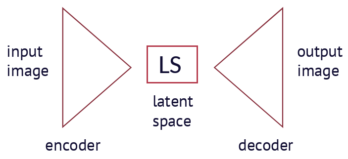
Figure 1: Autoencoder architecture.

2 Autoencoders

2.1 Autoencoder architecture

Autoencoders are neural networks which consist of encoder that encodes or compresses high-dimensional input data into low-dimensional LS and decoder that decodes or upscales LS representation for image reconstruction, as shown in Figure 1. Encoder and decoder usually consist of sequences of fully connected or convolutional layers. For many CV tasks AE can be trained in unsupervised manner simply by learning to reconstruct the input image. In this case Mean Square Error (MSE) loss is used as reconstruction loss function. This significantly simplifies training data processing and allows to use unlabeled data.

2.2 Variational Autoencoders

Variational autoencoders (VAE) are special probabilistic class of AEs. Encoder of VAE includes two additional layers with their outputs linked to mean $\mu$ and standard deviation $\sigma$ of the modeled distribution using (1) and (2) [11, 12]. Equation (1) shows that LS representation z in VAE contains random sampling from a normal distribution N(0,1) with zero mean and $\sigma=1$. Kullback-Leibler divergence (KLD) loss is calculated in addition to MSE loss to make LS distribution more like N(0,1). VAE is trained with combined loss consisting of weighted sum of KLD and MSE. During inference VAE outputs are sampled from a distribution similar to the input which is advantages for generators. The most notable VAE is UNet [13] which is widely used by Stable Diffusion [9] and other generative models.

$$z=\mu+\sigma\cdot N(0,1),$$ (1)

$$L_{KLD}=\mu^{2}+\sigma^{2}-log(\sigma)-0.5,$$ (2)

$$L=L_{MSE}+k_{d}\cdot L_{KLD},$$ (3)

where k_d is KLD weight coefficient.

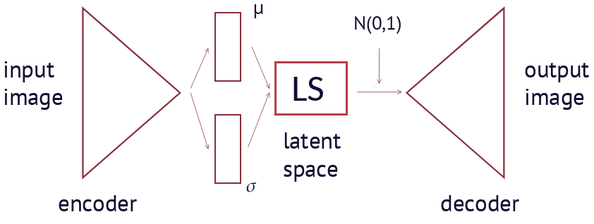
Figure 2: VAE architecture.

2.3 Supervised Autoencoders

Whereas AEs were initially proposed for unsupervised learning scenarios, they were proven useful for semi-supervised and supervised learning tasks, too. As any AE, SAE has encoder-decoder architecture with its decoder substituted by a classifier neural network. Decoder and classifier can also be used in parallel so that decoder output is used for regularization [14], but this use case is outside of the scope of this study. For supervised learning the reconstruction loss is substituted with classification loss most commonly being Cross Entropy (CE) loss. In this paper we study LS of SAE with architecture shown in Table 1 where Double layer means two subsequent sequences of convolution, batch normalization [15], and ReLU; and Down layer consists of MaxPool [16] followed by Double layer. This encoder architecture is inspired by VAE architecture [17] without (1) and (2) so dense layer outputs have no statistical meaning and can be referred to as a and b, so LS representation is z = a+b. Classifier is a simple 3-layer fully-connected network. Inference of such SAE is deterministic due to the absence of N(0,1) term in z.

Table 1: Studied SAE architecture.

Element	Layer	Parameter	Channels
Input	-	x	1,32,32
Encoder	Double(32->64)	-	64,32,32
	Down(64-128)	-	128,16,16
	Down(128-256)	-	256, 8, 8
	Down(256-512)	-	512, 4, 4
	Down(512-512)	-	512, 2, 2
	flatten	-	2048
	Lin(2048,2)	a	2
	Lin(2048,2)	b	2
LS	a + b	z	2
Classifier	Lin(2,32)	-	32
	Lin(32,64)	-	64
	Lin(64,5)	p	5
Output	argmax(p)	y	1

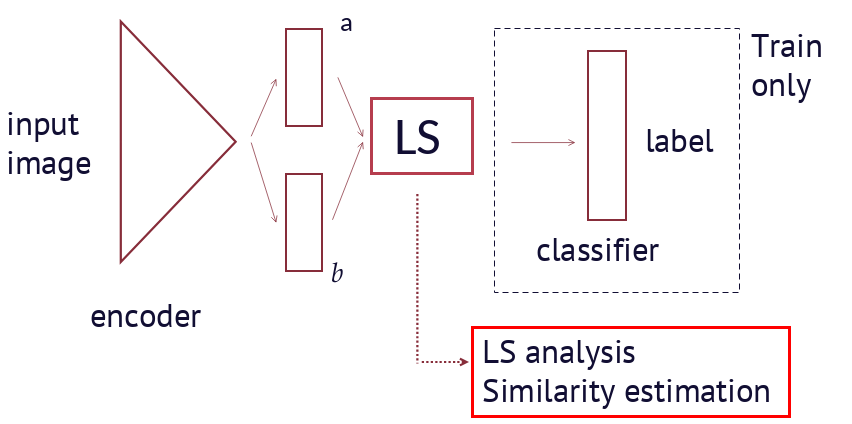
Figure 3: Conventional encoder-classifier SAE architecture to convert LS representation to label and the proposed direct LS analysis.

2.4 SAE latent space analysis

To predict label for a given input SAE first encodes it in LS and then uses classifier to produce the label from LS representation. However, LS representation, containing all the necessary information to predict the label, cannot be interpreted directly using conventional methods. To address this, it was previously proposed to use stochastic iterative algorithms to evaluate LS structure dynamically during training and possibly avoid using classifiers [18, 19, 20]. Our approach is similar to center loss [21] training with deterministic clusters and modified contributions of out-of-cluster samples to the loss function. In this paper we show that analyzing LS representation is possible when LS topology is known, and discuss means of obtaining the desired topology. We show in Section 6 that working with pre-configured LS allows to perform operations not readily available for conventional classifiers, such as similarity estimation for multiple inputs by analyzing their LS representations.

3 Latent space configuration methods

In this paper we propose two methods to configure LS in AE as shown in Figure 4 which are loss configuration and encoder configuration. The former can be considered as a special training procedure that allows to obtain LS with desired properties. The latter is more invasive since it changes the model in the same way adding $\mu$ and $\sigma$ layers does to AE to obtain VAE does.

3.1 Loss configuration

Figure 4 (a) illustrates that in loss configuration scenario a loss function called geometric loss (L_G) operates directly on LS and not on classifier output. Training is done with a loss function combining configuration loss with conventional CE or MSE loss, similar to KLD combined loss discussed in Section 2.2. This method does not require modifying the model, which can be an advantage when large pre-trained models are used and their fine-tuning is desired. Loss configuration is discussed in detail in Section 4 with experiment results presented in Section 5. The main drawback of this method is that loss condition is guaranteed only during training since loss function does not influence inference directly. This can be a problem for small datasets where training data does not contain the complete variability of possible inputs.

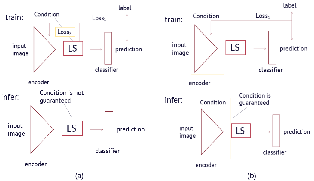
Figure 4: Differences between loss and encoder configuration.

3.2 Encoder configuration

Figure 4 (b) illustrates that the main advantage of encoder configuration is that it is guaranteed for inference. However, this requires implementing the condition as part of the encoder, which requires to modify the model. An example of such modification is the transition from AE to VAE discussed in Section 2. This method allows more control over the LS properties than loss configuration. For instance, polar coordinates or other transformations that completely change LS topology can be added. To illustrate this concept, SAE that uses polar coordinates in its encoder is studied. We aim to obtain LS with sectors each of which accommodates a specific class. We also add prohibited LS sectors such that if input is projected into the prohibited area, its LS position is modified to the next allowed sector by adding an extra rotation. For instance, for the case with 6 classes we define 50 degree class sectors with 10 degree prohibited sectors and an extra rotation of 30 degrees for points projected into prohibited regions. To achieve that an encoder of SAE in Table 1 is modified as

$$r=hypot(z[0],z[1]),$$ (4)

$$\phi=atan2(z[1],z[0]),$$ (5)

$$\phi^{\prime}=\begin{cases}\phi+\pi/6\ if\ (\phi\ mod\ \pi/3)\ mod\ 2\pi/9>\pi/18,\\ \phi\ otherwise;\end{cases}$$ (6)

$$z_{new}=concat(r\cdot cos(\phi^{\prime}),r\cdot sin(\phi^{\prime})).$$ (7)

It should be stressed that since the area prohibition is implemented in the encoder, no point can lie in prohibited areas of LS even during inference. For SAE described in Section 2.2 with modified encoder trained with L_CE we obtain LS distribution shown in Figure 5, where all clusters resemble beams heading outwards from the center.

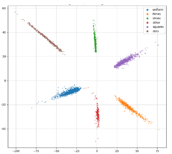
Figure 5: SAE trained with polar coordinate condition in encoder.

4 Geometric loss

In this paper we study a specific form of L_G that defines the positions and radii of clusters. Given the cluster center matrix C and cluster radius vector r_c, L_G is defined as

$$L_{G}=\sum_{i}^{n_{c}}\sum_{j}^{b_{s}}f_{d}(\sqrt{\sum_{k}^{n_{d}}(z_{jk}(y_{j}=i)-C_{ik})^{2}},r_{ci}),$$ (8)

where n_c is number of classes, b_s is number of samples in training batch, n_d is number of LS dimensions, i is class index, j is input sample index, k is LS dimension index, z_j is LS position and y_j is true label of j^th sample. f_d is a distance function defined as

$$f_{d}(x,r_{c})=exp(ReLU(x-r_{c}))-1.$$ (9)

Figure 6 shows f_d curve for r_c = 2 illustrating that this function is constant inside cluster and grows exponentially outside. It should be noted that adding a constant in (9) is not strictly necessary since derivative of any constant is zero, but we add -1 for convenience so f_d is exactly zero inside clusters.

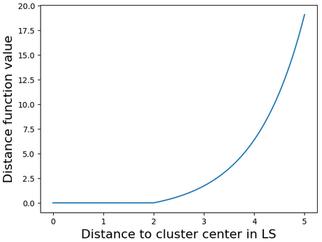
Figure 6: Curve of f_d function for r_c=2.

It is proposed to train SAE with a weighted combination of L_G and L_CE for classification with desired cluster locations. Therefore, combined loss for supervised training is

$$L=L_{CE}+k_{g}\cdot L_{G},$$ (10)

where k_g is geometric loss weight coefficient. In our experiments k_g = 0.2.

5 Configuring latent spaces for texture classification tasks

5.1 Texture classification on small datasets

In this paper we study LS of SAE designed for texture classification in context of person re-identification [22]. Its purpose is to substitute local binary pattern (LBP) [23] in our previously proposed method [24]. It should be noted that we do not conduct experiments on re-id benchmarks so re-id accuracy metrics are not reported in this study.

Since texture datasets for re-id are not available, a small dataset consisting of real clothes textures from LIP, internet stock photos, and images generated using a Stable Diffusion model [25] has been collected. Data is labeled into five classes: uniform (meaning no apparent texture), horizontal lines (hlines), vertical lines (vlines), checkered pattern (squares), and dots. We use dataset of as little as 130 images per class and apply a set of augmentations to artificially increase its size. The augmentations include rotations of up to 15 deg, perspective change, affine transformation, color jitter, and random erase of 30% of the image to simulate occlusion. Every augmented image is also accompanied by its vertical and horizontal mirror copies. We divide the dataset into 80% train / 20% test splits for training and testing and consider two testing scenarios: one with train-test sampling done before augmentation (about 130 images in test, no test image augmentation, “pre”-split in Table 2) and another one with sampling done after augmentation (about 300000 images in test, “post”-split in Table 2). In both cases the resulting training dataset consists of about 1.2 million train images, which is still quite small for a CV dataset. For generalization study we use 80 images from Market1501 which are low resolution and poor quality images representing worse case real world scenarios.

Table 2: Test and generalization accuracy for different random seed runs for SAE trained with different loss functions.

exp	LCE pre		LCE + LG pre		LCE post		LCE + LG post
	test	gen	test	gen	test	gen	test	gen
1	77	62	78	65	81	66	83	67
2	78	68	75	61	82	70	84	71
3	71	62	75	65	81	65	84	61

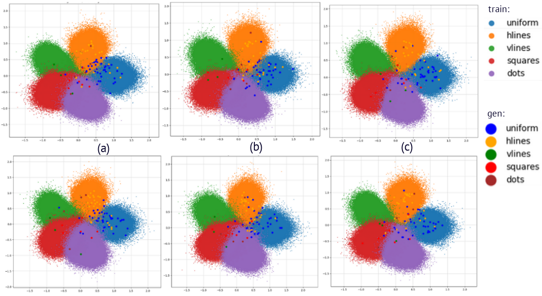
Figure 7: Positions of Market encodings in LS in L_CE + L_G experiments (a top), 1 pre (a bottom) 1 post, (b top) 2 pre, (b bottom) 2 post, (c top) 3 pre, (c bottom) 3 post.

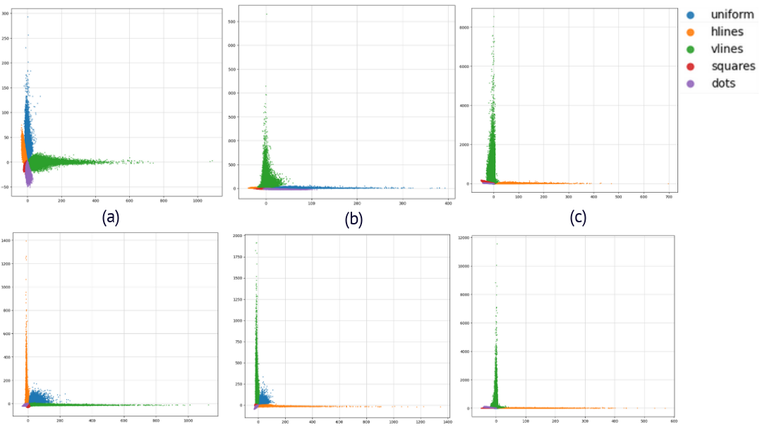
Figure 8: LS of SAE trained with L_CE, (a top) 1 pre, (a bottom) 1 post, (b top) 2 pre, (b bottom) 2 post, (c top) 3 pre, (c bottom) 3 post.

5.2 Conventional training and LS configuration training

Table 2 shows experimental results obtained by performing three runs with different random seeds fixed for four experiments constituting the run. Random variables include SAE initialization weights, train/test split samples, augmentation color jitter parameters, batch train data splits. All models are trained for 50 epochs with 1e-6 learning rate, with training accuracy exceeding 99% for all experiments. The classification results shown in Table 2 illustrate that test and Market1501 generalization accuracies are higher for the proposed training method. Using “post”-split in pre-processing also leads to better results.

Geometric loss configurations has the following parameters: five clusters n_c = 5 that are at d_c = 0.85 distance from center (0,0) and $2\pi/\textit{n\textsubscript{c}}$ = 72° angles relative to the neighbors with cluster radius r_c = 0.34. Figures 7 - 9 show positions of LS embeddings of train data (small points) with Figures 8 and 9 also showing Market generalization data LS embeddings (large points). Figure 7 (a) - (c) shows that L_CE + L_G training method allows to achieve the desired LS distributions for all experiments. Clusters resemble petals due to large number of points and the interplay between L_CE and L_G. Figure 7 shows that in all cases clusters appear in the desired positions with all training points being roughly inside a circle with radius two. All LS encodings in the Market transfer experiments also lie withing the specified regions not leaving the configured LS. This illustrates that even that LS condition is present only during training, the learned weights succeed in projecting new unseen data into the specified areas in LS.

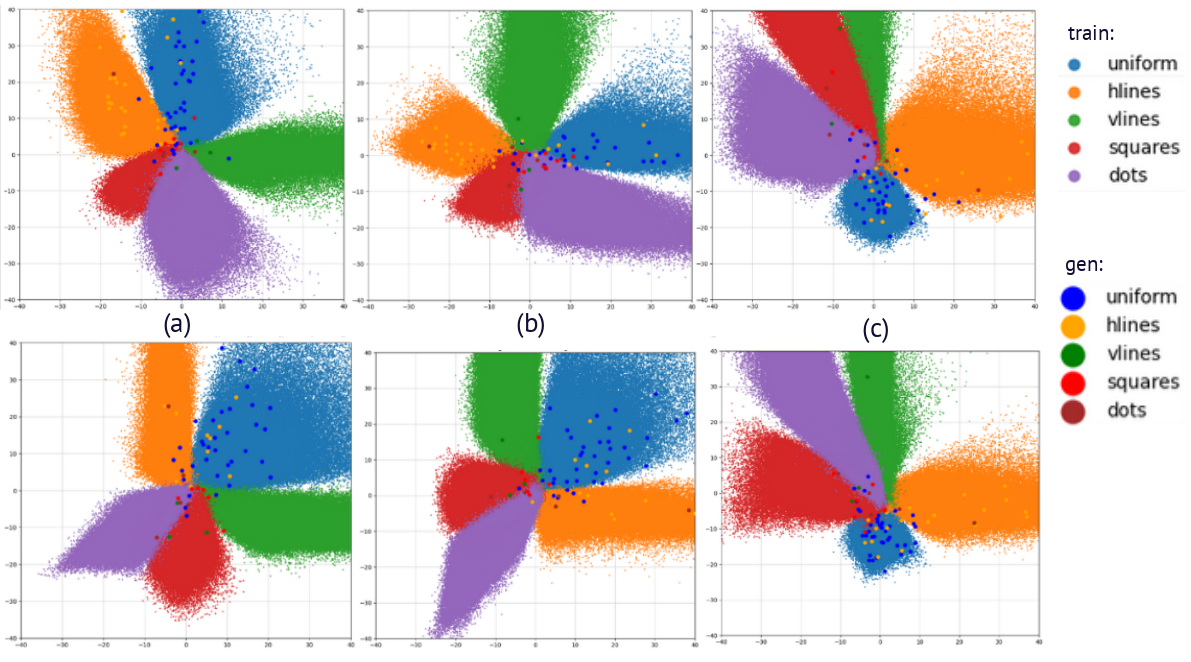
Figure 9: Positions of Market encodings in LS in L_CE experiments (a top), 1 pre (a bottom) 1 post, (b top) 2 pre, (b bottom) 2 post, (c top) 3 pre, (c bottom) 3 post.

On the contrary, for conventional training L_CE allows z to take any value and in this case, we can see huge “explosion” in LS positions along axes in Figure 8. Moreover, the LS shown in Figure 8 (a) - (f) are totally different. It is further illustrated by Figure 9 where [-40,40] regions are visualized. There is a high degree of asymmetry between clusters, and clusterization patterns are very different for different sets of random starting conditions. The comparison of Figures 7 and 9 shows positive effects of L_G on training making it more stable and predictable.

6 Image similarity estimation using LS analysis

6.1 Similarity in LS

Having information about cluster location and size that pre-configured LS provides can be an advantage for similarity estimation tasks. Since LS projections are confined into a compact space, we can estimate how similar the inputs are just by analyzing their positions and distances between their LS encodings. Conventional LS does not have this property since clusters have different shapes and their sizes are not predetermined, as Figures 8 and 9 illustrate.

To evaluate the similarity between two inputs we first propose to evaluate the similarity of each input to all classes by analyzing their LS positions relative to cluster centers. This allows to obtain class similarity vectors and then use these vectors to compare the inputs. To achieve that, vectors of cluster center distances d_i are calculated as Euclidean distances to cluster centers as

$$d_{ji}=\sqrt{\sum_{k}(z_{jk}-C_{ik})^{2}}.$$ (11)

They are used to calculate class similarity vectors as

$$v_{ji}=\begin{cases}1-k_{b}\cdot sin(\frac{d_{ji}}{r_{ci}})\ if\ d_{ji}\leq r_{ci},\\ ReLU(\frac{b_{c}\cdot(R_{d}-d_{ji})}{R_{d}-r_{ci}})\ otherwise;\\ \end{cases}$$ (12)

where b_c is a parameter corresponding to the desired similarity value at cluster boundary when d_ji = r_ji; k_b is calculated as

$$k_{b}=\frac{1-b_{c}}{sin(1)},$$ (13)

and is a constant for given b_c, and R_d is the distance between neighboring clusters

$$R_{d}=d_{c}\ \sqrt[]{2\cdot(1-cos(\frac{2\pi}{n_{c}}))}.$$ (14)

Cluster parameters in Section 5.2 yeild R_d = 1, and b_c = 0.79 in our experiments. Finally, for two points their similarity is calculated as

$$sim_{12}=\frac{\sum_{i}min(v_{1i},v_{2i})}{max(sum(v_{1}),sum(v_{2}))}.$$ (15)

6.2 LS similarity for texture retrieval

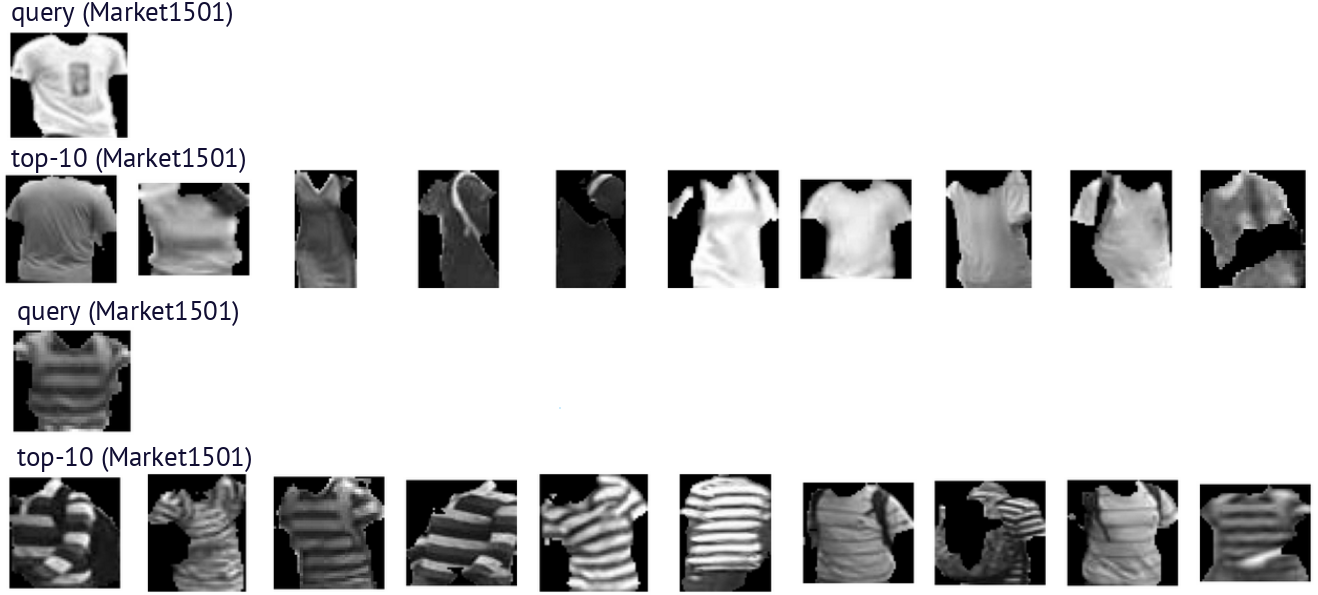
Figure 10: Examples of top-10 images matching texture of query image in Market1501 dataset.

Using the proposed similarity measure we can make similarity ranking of textures in LIP, Market1501, and Wildtrack datasets. It should be noted that LIP is a human parsing dataset, whereas Market1501 and WildTrack are re-id datasets. None of the datasets are specifically labeled for texture classification. Moreover, whereas subsets of LIP and Market1501 have been labeled as part of this study, WildTrack have not been labeled, which does not prevent us from creating similarity ranking thus surpassing the limitations of conventional classification methods. That is, whereas five classes have been used to train SAE, other class data can be analyzed with some degree of accuracy by estimating its similarity to the train classes.

It should be noted that only LS encodings are needed to conduct dataset search with the proposed method. Therefore, only one encoder forward pass is needed for each image in database, and LS encodings can be saved in the database along with images. Then, after query image is encoded and its LS encoding is known, it can be compared with database LS encodings directly. This is very fast and efficient since it reduces the involvement of NN in the analysis, and since ranking computations can easily be performed on general purpose CPU, this reduces the overall hardware requirements of the method.

Figure 10 shows top-10 clothes with textures most similar to the texture in query image (see Appendix A for more examples). It should be stressed that all results are obtained with SAE trained on our dataset and no retraining for specific datasets was conducted. This illustrates good generalization of the method to previously unseen data of different quality and type.

Figure 11 shows cross-dataset texture retrieval results where a similarity ranking for a query image from one dataset searched in another dataset is created (more in Appendix A). Specifically, queries from Market are searched in Wildtrack and vice versa using a model trained on data containing images from neither dataset. These examples show high visual similarity between the query and ten most similar images further illustrating great generalization capabilities of the proposed method. That is, images from very different cameras have been used for training and searching meaning that the model is trained to perform accurately over wide range of different lighting conditions and variations in image quality with no fine-tuning.

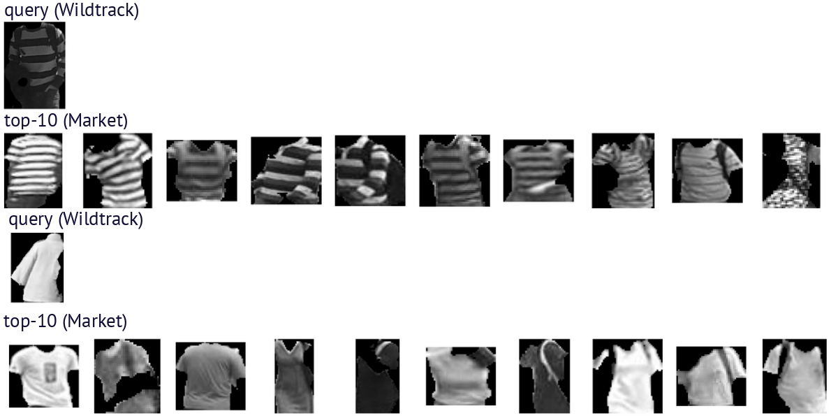
Figure 11: Top-10 similar images for Wildtrack query searched in Market1501.

6.3 Dataset search without a query image

We previously proposed an image retrieval method that allowed us to conduct database search using color description without query image [24]. It was done by creating feature vectors for typical colors and using such vectors in a search algorithm by comparing them to feature vectors of images stored in database. In this paper we show how the same principle can be used for texture search. Figure 12 shows how preconfigured LS can be used to correlate text queries with LS regions. Whereas it is possible to simply use cluster center locations as encodings, we can search for less clear examples to account for influence of specific cameras and lighting conditions by choosing a random point from relevant cluster. Furthermore, LS encodings can be estimated for texture types that are not in training classes as some combination of training class features.

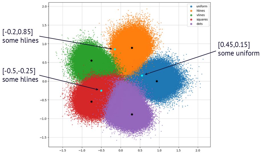
Figure 12: Example correlations between text queries and LS positions used for similarity search. Black dots correspond to configuration centers.

Figure 13 shows the retrieval results for points shown in Figure 12 (more examples in Appendix A). Uniform textures are retrieved with samples showing deviations from perfect uniform texture like folds and prints. In Figure A.4 horizontal line pattern textures are successfully retrieved from Market1501 apart from one sample with unclear texture due to low resolution. In Figure A.5 checked pattern coat has the highest score along with unspecified “rough” texture coats in Widltrack. It should be noted that due to low number of images in Wildtrack subset used for search there are simply very few images similar to the query. Nevertheless, the ability to access similarity with unlabeled unspecified textures is a great advantage of the proposed method.

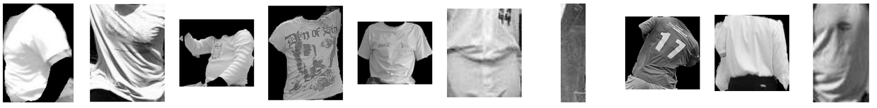
Figure 13: Search results for some uniform texture in training dataset.

7 Discussions

7.1 LS topology

In previous Sections we have shown that it is possible to add a relatively simple term to loss function to achieve a predefined configuration of LS during training. This allows to define location and size of the clusters which is then used to define an LS similarity measure to evaluate the similarity of different inputs based on their LS projections. Furthermore, Figure 7 shows that different training runs result in exactly the same LS train distribution for L_CE + L_G, whereas conventional training leads to strikingly different LS clusterization. Therefore, adding L_G term makes training more stable and predictable which in turn improves the interpretability of the results.

While in this paper the L_G was formulated for two-dimensional case for purposes of LS visualization on a 2D plane, it can be easily extended to n-dimensional cases. However, the possibility to directly affect the LS topology can have more profound implications. It is possible to obtain more “exotic” topologies with interesting properties through encoder configuration by guiding LS projection terms with special equations similar to (4)-(7). While this has been shown for polar coordinates, it is possible to obtain non-Euclidian spaces, for instance, hyperbolic spaces where distances between clusters are calculated in a completely different manner. The usefulness of this is not obvious and has to be studied in more detail.

7.2 Improved generalization with geometric loss

Sections 5 and 6 have shown better generalization of SAE trained with L_G. This can be partly explained by more structured and compact LS. It should be mentioned that test accuracy is not very high for both conventional and proposed training methods because of the small dataset size. That is, there is a possibility that test set contains samples significantly different from the train set simply due to the high variance among data samples. There also are significant challenges for texture classification due to the inherent similarity between certain classes. The analysis of the incorrect classifications has shown that folds on uniform texture often get misclassified as vertical or horizontal line patterns, and sometimes patterns of squares and dots might become indistinguishable due to low resolution of input images (see Table 2). This can be attributed to the nature of the experiment used in this study and not to the proposed LS configuration methodology.

High generalization of the method is also illustrated by Figure 11 where images from one dataset are used as queries for search in another dataset. It should be stressed again that for both experiments SAE was trained on third dataset, indicating that the proposed method can work in real-world scenarios where neither database images nor new images obtained from cameras can be used for training. The proposed geometric clusterization in combination with the proposed similarity estimation method has an emerging property of the ability to access similarity for classes that are not in training class set. When given a completely new texture, SAE encodes it in LS as any other input, and its position depends on its similarity to train classes via proximity to class clusters. Conventional SAE classifier then outputs a label which is contained in training classes’ set thus being unable to predict an unseen class. However, given a pair of unseen class inputs the proposed method can access their similarity directly from their LS positions, giving high similarity score to similar inputs. This is a significant advantage of the proposed method when input similarity estimation rather than classification is to be performed.

7.3 Text query search without a language model

In Section 6.3 we have shown that we can estimate regions of LS where certain types of textures are likely to be. This is possible since we have configured LS in a predefined manner. This allows us to establish correspondence between verbal or text descriptions of textures and LS regions. The results in Figure 13, A.4, and A.5 that show the successful text query search for different datasets illustrate good generalization capabilities. Hence, a necessity to process natural language with a separate model to create text embeddings is removed. This idea can be extended to generative models, too, in order to reduce the number of components and improve interpretability. However, this would require training a diffusion model with L_G and preconfiguring LS with n_d much larger than 2, e.g. 4096 for conventional VAEs. The means of achieving this are not obvious and this topic will be studied in the future.

8 Conclusions

This paper proposes two methods for LS configuration for SAE. The first method implements geometric loss term which guides training to create the desired configuration of the LS. The second method modifies SAE encoder to alter LS properties. It has the potential to provide unprecedented control over LS properties and guarantees the desired behavior during inference. However, it causes difficulties during training which will be studied in the future. For the former it is shown that training with the proposed geometric loss reliably leads to the desired LS configuration while making training more stable and interpretable. It also leads to higher generalization accuracy, as shown by clothes texture classification task results for SAE trained on a small custom dataset and tested on subsets from datasets LIP, Market1501, and WildTrack. Using LS configuration also allows to define a similarity measure directly in LS to access similarity of multiple inputs without classifier. This is used to create similarity ranking and search for images with textures similar to a given query image. High generalization of the proposed method is illustrated by successful inter- and cross-dataset searches where a model trained on one dataset is used to search for a query from second dataset in third dataset. Finally, known LS configuration is used to correspond text queries to LS positions and conduct database search without query images and language models.

Data availability

Training data used in this study can be provided on request addressed to the corresponding author.

Appendix A Appendix 1

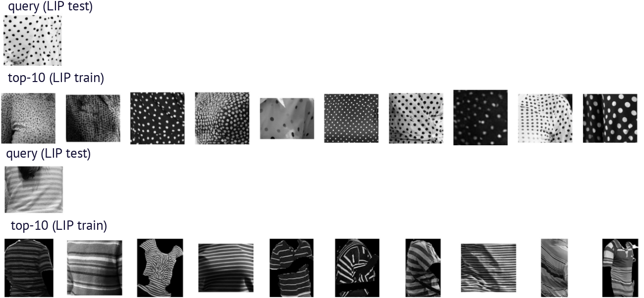
Figure A.1: Examples of top-10 images matching texture of query image from LIP test searched in LIP train subsets.

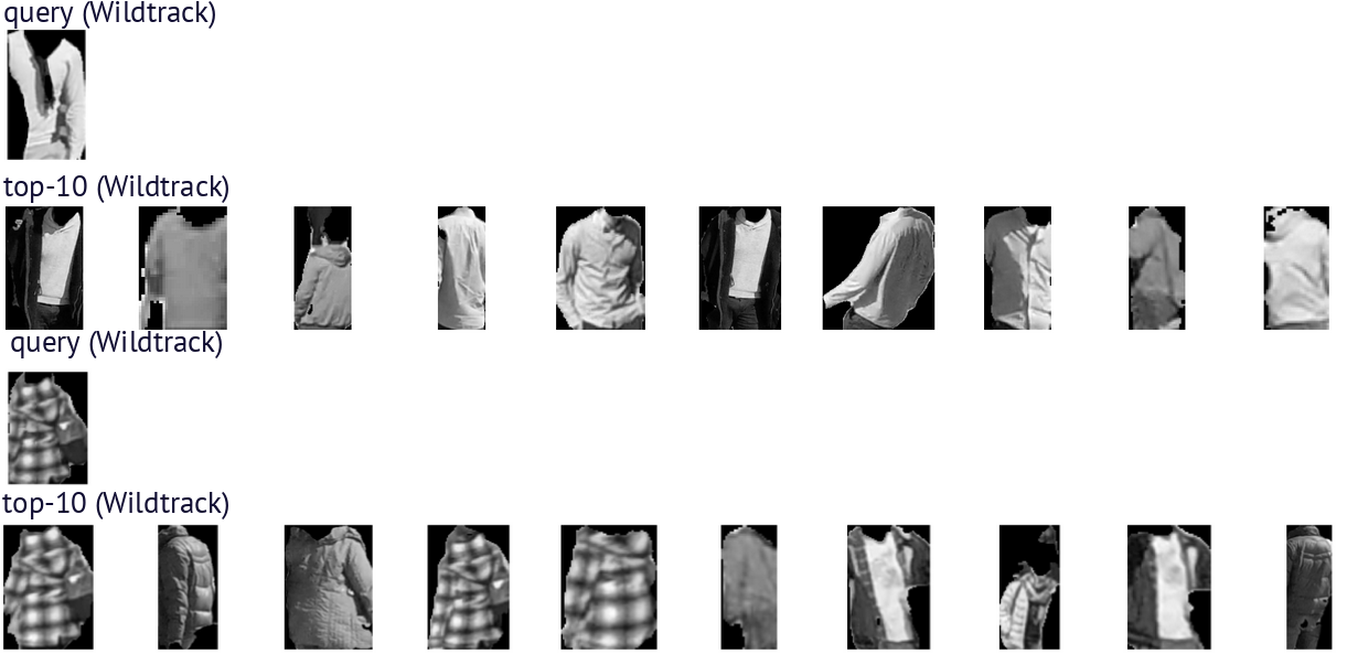
Figure A.2: Examples of top-10 images matching texture of query image on Wildtrack dataset.

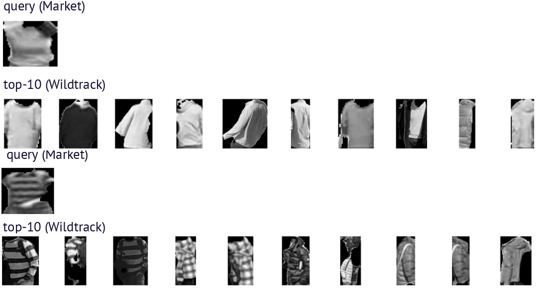
Figure A.3: Top-10 similar images for Marhet1501 query searched in Wildtrack.

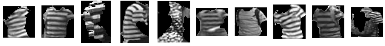
Figure A.4: Search results for some horizontal lines texture in Market1501 dataset.

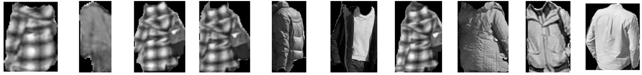
Figure A.5: Search results for textures with checkered pattern in Wildtrack dataset.

References

- [1] K. G. Lore, A. Akintayo, and S. Sarkar, “Llnet: A deep autoencoder approach to natural low-light image enhancement,” 2016. [Online]. Available: https://arxiv.org/abs/1511.03995
- [2] X.-J. Mao, C. Shen, and Y.-B. Yang, “Image restoration using convolutional auto-encoders with symmetric skip connections,” 2016. [Online]. Available: https://arxiv.org/abs/1606.08921
- [3] X. J. Guijuan Zhang, Yang Liu, “A survey of autoencoder-based recommender systems,” Frontiers of Computer Science, vol. 14, no. 2, p. 430, 2020. [Online]. Available: https://journal.hep.com.cn/fcs/EN/abstract/article_23822.shtml
- [4] H. S. Vu, D. Ueta, K. Hashimoto, K. Maeno, S. Pranata, and S. M. Shen, “Anomaly detection with adversarial dual autoencoders,” 2019. [Online]. Available: https://arxiv.org/abs/1902.06924
- [5] D. Bank, N. Koenigstein, and R. Giryes, “Autoencoders,” 2021. [Online]. Available: https://arxiv.org/abs/2003.05991
- [6] K. Gong, X. Liang, D. Zhang, X. Shen, and L. Lin, “Look into person: Self-supervised structure-sensitive learning and a new benchmark for human parsing,” in 2017 IEEE Conference on Computer Vision and Pattern Recognition (CVPR), 2017, pp. 6757–6765.
- [7] L. Zheng, L. Shen, L. Tian, S. Wang, J. Wang, and Q. Tian, “Scalable person re-identification: A benchmark,” in 2015 IEEE International Conference on Computer Vision (ICCV), 2015, pp. 1116–1124.
- [8] T. Chavdarova, P. Baqué, S. Bouquet, A. Maksai, C. Jose, T. Bagautdinov, L. Lettry, P. Fua, L. Van Gool, and F. Fleuret, “Wildtrack: A multi-camera hd dataset for dense unscripted pedestrian detection,” in IEEE/CVF Conference on Computer Vision and Pattern Recognition, 2018, pp. 5030–5039.
- [9] R. Rombach, A. Blattmann, D. Lorenz, P. Esser, and B. Ommer, “High-resolution image synthesis with latent diffusion models,” 2022. [Online]. Available: https://arxiv.org/abs/2112.10752
- [10] A. Radford, J. W. Kim, C. Hallacy, A. Ramesh, G. Goh, S. Agarwal, G. Sastry, A. Askell, P. Mishkin, J. Clark, G. Krueger, and I. Sutskever, “Learning transferable visual models from natural language supervision,” 2021. [Online]. Available: https://arxiv.org/abs/2103.00020
- [11] D. P. Kingma and M. Welling, “An introduction to variational autoencoders,” 2019. [Online]. Available: https://arxiv.org/abs/1906.02691
- [12] D. Kingma and M. Welling, “Auto-encoding variational bayes,” 2022. [Online]. Available: https://arxiv.org/abs/1312.6114
- [13] O. Ronneberger, P. Fischer, and T. Brox, “U-net: Convolutional networks for biomedical image segmentation,” 2015. [Online]. Available: https://arxiv.org/abs/1505.04597
- [14] L. Le, A. Patterson, and M. White, “Supervised autoencoders: Improving generalization performance with unsupervised regularizers,” in Advances in Neural Information Processing Systems, vol. 31, 2018, pp. 107–117.
- [15] S. Ioffe and C. Szegedy, “Batch normalization: Accelerating deep network training by reducing internal covariate shift,” 2015. [Online]. Available: https://arxiv.org/abs/1502.03167
- [16] H. Gholamalinezhad and H. Khosravi, “Pooling methods in deep neural networks, a review,” 2020. [Online]. Available: https://arxiv.org/abs/2009.07485
- [17] (2024) Pytorch implementation of unet. Date Accessed: 31-01-2024. [Online]. Available: https://github.com/milesial/Pytorch-UNet
- [18] Q. Zhu and R. Zhang, “A classification supervised auto-encoder based on predefined evenly-distributed class centroids,” 2020. [Online]. Available: https://arxiv.org/abs/1902.00220
- [19] C.-H. Pham, S. Ladjal, and A. Newson, “Pcaae: Principal component analysis autoencoder for organising the latent space of generative networks,” 2020. [Online]. Available: https://arxiv.org/abs/2006.07827
- [20] H. Luo, W. Jiang, Y. Gu, F. Liu, X. Liao, S. Lai, and J. Gu, “A strong baseline and batch normalization neck for deep person re-identification,” IEEE Transactions on Multimedia, vol. 22, no. 10, p. 2597–2609, Oct. 2020. [Online]. Available: http://dx.doi.org/10.1109/TMM.2019.2958756
- [21] Y. Wen, K. Zhang, Z. Li, and Y. Qiao, “A discriminative feature learning approach for deep face recognition,” in ECCV 2016, B. Leibe, J. Matas, N. Sebe, and M. Welling, Eds., 2016, pp. 499–515.
- [22] L. Zheng, Y. Yang, and A. G. Hauptmann, “Person re-identification: Past, present and future,” 2016. [Online]. Available: https://arxiv.org/abs/1610.02984
- [23] T. Ahonen, A. Hadid, and M. Pietikainen, “Face description with local binary patterns: Application to face recognition,” IEEE Transactions on Pattern Analysis and Machine Intelligence, vol. 28, no. 12, pp. 2037–2041, 2006.
- [24] N. Gabdullin, “Combining human parsing with analytical feature extraction and ranking schemes for high-generalization person reidentification,” Applied Sciences, vol. 13, no. 3, 2023. [Online]. Available: https://www.mdpi.com/2076-3417/13/3/1289
- [25] L. Zhang. (2024) Fooocus. Date Accessed: 31-01-2024. [Online]. Available: https://github.com/lllyasviel/Fooocus