Distribution Estimation under the Infinity Norm

Abstract

We present novel bounds for estimating discrete probability distributions under the $\ell_{\infty}$ norm. These are nearly optimal in various precise senses, including a kind of instance-optimality. Our data-dependent convergence guarantees for the maximum likelihood estimator significantly improve upon the currently known results. A variety of techniques are utilized and innovated upon, including Chernoff-type inequalities and empirical Bernstein bounds. We illustrate our results in synthetic and real-world experiments. Finally, we apply our proposed framework to a basic selective inference problem, where we estimate the most frequent probabilities in a sample.

Keywords: Distribution Estimation, Probability Estimation, Infinity Norm

1 Introduction

Consider a probability distribution $p$ over $\mathbb{N}=\left\{1,2,\ldots\right\}$. Let $X^{n}$ be a sample of $n$ independent observations from $p$. In this work we study the basic problem of estimating $p$ from $X^{n}$. We focus our attention to the infinity norm, which is formally defined in (4). Also known as the uniform or supremum norm, this popular metric over distributions has a number of important applications — in addition to being a fundamental object of independent interest (Boucheron et al., 2003; Van Handel, 2014). Among the applications is a selective inference scheme for multinomial proportions, as discussed below.

Our reference point is the following simple and classic bound, whose proof is an easy consequence of McDiarmid’s inequality: for all $\delta\in(0,1)$,

$$\sup_{i\in\mathbb{N}}|p_{i}-\hat{p}_{i}(X^{n})|\lesssim\sqrt{\frac{\log(1/\delta)}{n}}$$ (1)

holds with probability at least $1-\delta$, where $\hat{p}_{i}(X^{n})$ is the maximum likelihood estimator (MLE) defined below and $\lesssim$ hides small absolute constants. This rate is known to be tight in the worst case (Lemma 17), but can certainly be improved upon for benign distributions. For example, when $p=(1-\theta,\theta)$ is the Bernoulli distribution, Bernstein’s inequality (Boucheron et al., 2003, Corollary 2.11) yields

$$|\theta-\hat{\theta}|\lesssim\sqrt{\frac{\theta(1-\theta)}{n}\log\frac{1}{\delta}}+\frac{1}{n}\log\frac{1}{\delta},$$ (2)

where $\hat{\theta}$ is the MLE. Furthermore, (2) has an empirical Bernstein version (Dasgupta and Hsu, 2008a, Lemma 5), in which the unknown quantity $\theta$ is replaced in the right-hand side by the empirically computable $\hat{\theta}$.

Drawing inspiration from (2) and its empirical version, we might expect something like

$$\sup_{i\in\mathbb{N}}|p_{i}-\hat{p}_{i}(X^{n})|\stackrel{{\scriptstyle?}}{{\lesssim}}\sqrt{\frac{v^{*}\log\frac{1}{\delta}}{n}}+\frac{1}{n}\log\frac{1}{\delta},$$ (3)

where $v^{*}=\max_{i\in\mathbb{N}}p_{i}(1-p_{i})$, or, even more ambitiously, some version of (3) with $v^{*}$ replaced by its empirical version $\hat{v}^{*}$. It will turn out that (3) is too optimistic. Absent an oracle that tells us the index of the largest mass, some additional cost must be incurred for estimating many symbol probabilities simultaneously.

Our contributions.

Our main result amounts to nearly achieving the ultimate goal. First, we derive a Chernoff-type upper bound in Thereom 1, which improves upon (1). Theorem 2 introduces its data-dependent counterpart, which demonstrates a significant improvement in small sample regimes. Next, we establish in Theorem 3 a version of (3) where $v^{*}$ is replaced by $v^{*}\log\frac{1}{v^{*}}$ and provide even sharper bounds therein. These are matched by nearly optimal lower bounds, in distinct senses made precise below. Finally, we apply our results to the important problem of selective inference. Specifically, we study the basic problem of inferring the most frequent events in a sample and achieve a significant improvement over currently known schemes.

2 Definitions and Problem Statement

Consider a probability distribution $p$ over $\mathbb{N}$, which induces the random variable $X\sim p$. The support size of $X$, $||p||_{0}$, is also the alphabet size — and unless stated otherwise, our results hold even when these are infinite. Let $X^{n}=(X_{1},...,X_{n})$ be a sample consisting of $n$ independent copies of $X$. Let $c_{i}(X^{n})$ be the count (number of appearances) of the $i^{th}$ symbol in the sample. Let $\hat{p}(X^{n})$ be the maximum likelihood estimator (MLE) of $p$; namely, $\hat{p}_{i}(X^{n})=c_{i}(X^{n})/n$ for every $i\in\mathbb{N}$. In this work, we study empirical distribution estimation of $p$ under the infinity norm. That is, given a prescribed $\delta>0$, we seek a random variable $T_{\delta}(X^{n})$ such that

$$||p-\hat{p}(X^{n})||_{\infty}\triangleq\sup_{i\in\mathbb{N}}|p_{i}-\hat{p}_{i}(X^{n})|\leq T_{\delta}(X^{n})$$ (4)

with probability of at least $1-\delta$. In light of (1), we also require that, for fixed $\delta$, $T_{\delta}(X^{n})\to 0$ as $n\to\infty$, in some appropriate sense.

Notice that (4) may also be viewed as a multinomial inference scheme. Specifically, (4) implies that $p_{i}\in[\hat{p}_{i}\pm T(X^{n})]$ simultaneously for all $i\in\mathbb{N}$. This confidence region (CR) defines a hypercube around the MLE, which covers $p$ with a confidence level of $1-\delta$.

3 Related Work

Discrete probability estimation is a fundamental problem in many fields. It is extensively studied under a variety of merits such as total variation (Jiao et al., 2017; Cohen et al., 2020), KL divergence (Orlitsky and Suresh, 2015), Hellinger distance (Hellinger, 1909) Wasserstein metric (Kantorovich, 1960), Kolmogorov-Smirnov distance (Smirnov, 1948) and others. The interested reader is referred to (Rice, 2006; Painsky and Wornell, 2019; Painsky, 2023b) for a comprehensive discussion. In this work we focus on the infinity norm. Here, the baseline is the bound implicit in (1), where, in the language of (4), $T_{\delta}(X^{n})=\sqrt{{1}/{n}}+\sqrt{{\log(1/\delta)}/{2n}}$.

The infinity norm is difficult to analyze in the general case (4). In fact, it is later shown (Section 4) that (1) is only asymptotically tight and only for the worst-case distribution, and can be significantly improved in a limited sample regime. On the other hand, the binomial case, $||p||_{0}=2$, is fairly understood as far as minimax optimal and fully empirical bounds. In particular, if $Y\sim\text{Bin}(n,\theta)$ is a Binomial random variable and $\hat{\theta}=Y/n$ its MLE, then Bousquet et al. (2003) and later Dasgupta and Hsu (2008b) showed that

$$|\theta-\hat{\theta}|\leq\sqrt{\frac{5\hat{\theta}(1-\hat{\theta})}{n}\log\frac{2}{\delta}}+\frac{5}{n}\log\frac{2}{\delta}$$ (5)

with probability of at least $1-\delta$. A closely related line of work appears in the statistics literature. Let $F(y;n,\theta)$ be the cumulative distribution function of $Y$. For a given $y$ and $n$, let $\theta_{l}$ and $\theta_{u}$ be the solutions (with respect to $\theta$) of $F(y;n,\theta)=\delta/2$ and $F(y;n,\theta)=1-\delta/2$ respectively. Clopper and Pearson (1934) showed that

$$\mathbb{P}\left(\theta\in[\theta_{l},\theta_{u}]\right)\geq 1-\delta$$ (6)

for every $\theta\in[0,1]$. The interval $[\theta_{l},\theta_{u}]$ is widely known as the exact Clopper-Pearson (CP) confidence interval (CI). The exact notion refers to the fact that (6) holds for every $n$, as opposed to alternative approximations. In fact, CP is also known to be shortest possible CI, for most setups of interest. Specifically, let $\mathcal{T}$ be a collection of intervals $[t_{l},t_{u}]$ that satisfy $\mathbb{P}\left(\theta\in[t_{l},t_{u}]\right)\geq 1-\delta$, for every $[t_{l},t_{u}]\in\mathcal{T}$. The shortest CI for $\theta$ is defined as the intersection of all intervals in $\mathcal{T}$. This notion also implies minimal expected length and minimal false coverage probability, uniformly. Wang (2006) showed that for $n\geq\log(\delta/2)/\log 0.5$, the CP CI is the shortest. Notice that for a nominal level of $\delta=0.05$, this condition corresponds to $n\geq 6$. Hence, for practical setups of interest, the CP interval $[\theta_{l},\theta_{u}]$ is the shortest possible CI for $\theta$. Unfortunately, CP does not hold a closed-form expression. Yet, Thulin (2014) showed that for every $y\in\{1,...,n-1\}$,

$$\theta_{l}=\hat{\theta}-z_{\frac{\delta}{2}}\sqrt{\frac{\hat{\theta}(1-\hat{\theta})}{n}}+\frac{1}{3n}\left(\left(1-2\hat{\theta}\right)z_{\delta/2}^{2}-1-\hat{\theta}\right)$$

$$\theta_{u}=\hat{\theta}+z_{\frac{\delta}{2}}\sqrt{\frac{\hat{\theta}(1-\hat{\theta})}{n}}+\frac{1}{3n}\left(\left(1-2\hat{\theta}\right)z_{\delta/2}^{2}+2-\hat{\theta}\right)$$

up to additive terms of order $n^{-3/2}$, where $z_{\delta}/2$ is the upper $\delta/2$ quantile of the standard normal distribution. This result implies that for every $y\in\{1,...,n-1\}$, the shortest possible CI length for $\theta$ is

$$\theta_{u}-\theta_{l}=2z_{\delta/2}\sqrt{{\hat{\theta}(1-\hat{\theta})}/{n}}+{1}/{n}+O(n^{-3/2}).$$ (7)

Moreover, we have

$$|\theta-\hat{\theta}|\leq\max\{|\hat{\theta}-\theta_{l}|,|\hat{\theta}-\theta_{u}|\}$$ (8)

with probability of at least $1-\delta$. Importantly, it can be shown that $z_{\delta/2}$ behaves asymptotically like $\sqrt{2\log(2/\delta)}$. Comparing (1) to (8) (and (5)) , we observe that its sample complexity, $1/\sqrt{n}$, is tight. However, there may still be room for improvement by utilizing a data-dependent scheme.

The Clopper-Pearson interval (8) provides a tight solution for the binomial case $||p||_{0}=2$. Yet, the problem becomes more involved in the multinomial setting (4). Currently known methods focus on two basic regimes. The first considers an asymptotic setup, where $n$ is much greater than the alphabet size (Quesenberry and Hurst, 1964; Goodman et al., 1964; Sison and Glaz, 1995). The second addresses the case where both $n$ and $||p||_{0}$ are small (Chafai and Concordet, 2009; Malloy et al., 2020). Notice that while some of these methods provide rectangular CR (Quesenberry and Hurst, 1964; Goodman et al., 1964; Painsky, 2023a; Marton and Painsky, 2024), others focus on hyper-cubes (Sison and Glaz, 1995). Yet, all of these methods assume a finite alphabet where performance guarantees are limited to relatively small $||p||_{0}$. To the best of our knowledge, no method considers the case where $||p||_{0}$ may be infinite.

4 Main Results

We begin our analysis by considering a data-indepedent bound under the infinity norm. Our proposed bound generalizes (1) by utilizing a Chernoff-like concentration bound.

Theorem 1.

Let $p=p_{i\in\mathbb{N}}$ be a distribution over $\mathbb{N}$. Let $X^{n}$ be a sample of $n$ independent observations from $p$. Let $\hat{p}(X^{n})$ be the MLE of $p$. Then, with probability $1-\delta$,

$$\left\|p-\hat{p}\right\|_{\infty}= \sup_{i\in\mathbb{N}}|p_{i}-\hat{p}_{i}(X^{n})|\leq\frac{1}{n}\left(\frac{1}{\delta^{1/m}}\right)\sum_{k=1}^{m/2}\left(k^{m-k}n^{k}\sum_{i\in\mathcal{X}}p_{i}^{k}(1-p_{i})^{k}\right)^{1/m}\leq$$ (9)

$$\frac{1}{\sqrt{n}}\frac{\sqrt{m/2}}{\delta^{1/m}}\exp\left(-\frac{1}{2}+\frac{1}{m}\right)+O\left(\frac{1}{n^{\frac{1}{2}+\frac{1}{m}}}\right)$$

for every even $m>0$.

Theorem 1 relies Markov’s inequality for higher-order moments of the infinity norm. In addition, it applies higher-order properties of the MLE and the binomial distribution. The detailed proof appears in Section 8.1. Next, similarly to Chernoff inequality, we minimize (9) with respect to $m$ to obtain tighter convergence guarantees. Specifically, we minimize the leading term of (9) to obtain

$$\min_{m\in\mathbb{R}^{+}}\frac{\sqrt{m/2}}{\delta^{1/m}}\exp\left(-\frac{1}{2}+\frac{1}{m}\right)=\sqrt{1+\log\left(\frac{1}{\delta}\right)}$$ (10)

for the choice $m^{*}=2\log(1/\delta)+2$ (See Appendix C). Hence the infimum of the bound is given by

$$\sqrt{\frac{1+\log\left({1}/{\delta}\right)}{n}}+O\left(\frac{1}{n^{\frac{1}{2}+\frac{1}{m^{*}}}}\right).$$ (11)

Unfortunately, this is not a great improvement over the benchmark (1). However, it is shown in Section 8.1 that as $m$ increases, the second inequality in (9) becomes tight for a worst-case case distribution $p=[1/2,1/2,0,\dots,0]$. This distribution is quite “unlikely” in a large alphabet regime. On the other hand, if we assume a “more likely” uniform distribution over a finite alphabet size $A:=||p||_{0}<\infty$, we obtain

$$\left\|p-\hat{p}\right\|_{\infty}\leq\frac{1}{\sqrt{n}}\frac{\sqrt{m/2}}{\delta^{1/m}}A^{-\frac{1}{2}+\frac{1}{m}}+O\left(\frac{1}{n^{\frac{1}{2}+\frac{1}{m}}}\right)$$

for every even $m>0$. Minimizing the leading term with respect to $m$ yields

$$\min_{m\in\mathbb{R}^{+}}\frac{\sqrt{m/2}}{\delta^{1/m}} A^{-\frac{1}{2}+\frac{1}{m}}=\sqrt{\log\left(\frac{A}{\delta}\right)}\exp\left(\frac{1}{2}-\frac{1}{2}\log(A)\right),$$ (12)

for the choice $m^{*}=2\log(A/\delta)$. Notice the above vanishes with $A$. This result motivates our quest for a data-dependent bound, which considers an empirical estimate of $p$ and does not assume a worst-case distribution as in (1) and (11). Theorem 2 below improves upon (9) and introduces a data-dependent bound which further accounts for $\hat{p}$.

Theorem 2.

Let $\delta_{1}>0$ and $\delta_{2}>0$. Let $m$ be a positive even number. Then, with probability $1-\delta_{1}-\delta_{2}$,

$$\left\|p-\hat{p}\right\|_{\infty}\leq\frac{1}{n}\left(\frac{1}{\delta_{1}}\frac{n}{n-1}\left(\sum_{i}\sum_{k=1}^{m/2}k^{m-k}n^{k}(\hat{p}_{i}(1-\hat{p}_{i}))^{k}+\epsilon\right)\right)^{1/m}$$ (13)

for every even $m$, where

$$\epsilon=\sqrt{\frac{n}{2}\log(1/\delta_{2})}\cdot\sum_{k=1}^{m/2}k^{m-k}n^{k}\left(\frac{k}{n4^{k-1}}+\frac{3k^{3}}{n^{3}2^{2k-5}}\right).$$

To prove of Theorem 2 we utilize the first inequality of (9) with $\delta=\delta_{1}$. Then, we apply McDiarmind’s inequality to obtain a concentration bound for $\sum_{i\in\mathbb{N}}p_{i}^{k}(1-p_{i})^{k}$ around its empirical counterpart, with probability $1-\delta_{2}$. Finally, we apply the union bound to obtain (13). The detailed proof is provided in Section 8.2. To further clarify the proposed bound we introduce the following simplified corollary, whose proof is located in Section 8.2.1.

Corollary 2.1.

Let $\delta_{1}>0$ and $\delta_{2}>0$. Let $m$ be a positive even number. Then, with probability $1-\delta_{1}-\delta_{2}$,

$$\left\|p-\hat{p}\right\|_{\infty}\leq$$

$$\frac{m}{\delta_{1}^{1/m}}\frac{1}{n}\left(\sum_{k=1}^{m/2}\sum_{i}(n\hat{p}_{i}(1-\hat{p}_{i}))^{k}\right)^{1/m}+a\frac{m}{\delta_{1}^{1/m}}\left(\log\left(\frac{1}{\delta_{2}}\right)\right)^{1/2m}\left(\frac{1}{n^{\frac{1}{2}\left(1+\frac{1}{m}\right)}}+\frac{24}{n^{\frac{1}{2}\left(1+\frac{5}{m}\right)}}\right)$$

for every even $m$, where $a=\sqrt{2\exp(1/\mathrm{e})}$. Furthermore,

$$\inf_{m}\frac{m}{\delta_{1}^{1/m}}=\mathrm{e}\log(1/\delta_{1}),$$

where and the infimum is obtained for a choice of $m^{*}=\log(1/\delta_{1})$.

Let us compare Corollary 2.1 with the benchmark scheme (1) and our previous data independent bound (Theorem 1). First, we notice a similar sample complexity of order of $\sqrt{1/n}$ in all the three schemes. This is not quite surprising, given (5). However, Corollary 2.1 demonstrates an improved dependency on the underlying distribution, which now depends on $\hat{p}$ and does not assume a worst-case distribution. Unfortunately, the dependency in $\hat{p}$ is somewhat involved, and does not hold the desired form of (3). Finally, we compare the dependency in the confidence level $\delta$. Here, the data independent bounds introduce a squared root logarithmic dependency in $1/\delta$. On the other hand, Corollary 2.1 only attains a logarithmic dependency in $1/\delta_{1}$ (where $\delta_{1}<\delta$) for the right choice of $m$. This difference is typically negligible compared to the other terms, especially in a fixed $\delta$ regime as later discussed.

Next, we present our second main result, which introduces a dependency in $p$ that is closer to the desired form (3). First, we introduce some additional notation.

Notation.

For any distribution $p_{i\in\mathbb{N}}$, define $v=v(p)$ by $v_{i}=p_{i}(1-p_{i})$ and $v^{*}=\max_{i\in\mathbb{N}}v_{i}$ as above. Define the functional

$$V^{*}(p)=\sup_{i\in\mathbb{N}}v_{i}(p^{\downarrow})\log(i+1),$$ (14)

where $p^{\downarrow}$ is $p$ sorted in non-increasing order. Define

$$\varphi(t)=t\log\frac{1}{t},\qquad 0\leq t\leq 1.$$ (15)

Theorem 3.

Let $p=p_{i\in\mathbb{N}}$ be a distribution over $\mathbb{N}$ and put $v^{*}=v^{*}(p)$, $V^{*}=V^{*}(p)$. For $n\geq 81$ and $\delta\in(0,1)$, we have that

$$\left\|p-\hat{p}\right\|_{\infty}\leq 2\sqrt{\frac{V^{*}}{n}+\frac{v^{*}}{n}\log\frac{2}{\delta}}+\frac{4}{3n}\log\frac{2(n+1)}{\delta}+\frac{\log n}{n}\leq$$ (16)

$$2\sqrt{\frac{\varphi(v^{*})}{n}+\frac{v^{*}}{n}\log\frac{2}{\delta}}+\frac{4}{3n}\log\frac{2(n+1)}{\delta}+\frac{\log n}{n};$$ (17)

$$\left\|p-\hat{p}\right\|_{\infty}\leq 2\sqrt{\frac{v^{*}\log(n+1)}{n}+\frac{v^{*}}{n}\log\frac{2}{\delta}}+\frac{4}{3n}\log\frac{2(n+1)}{\delta}+\frac{\log n}{n}$$ (18)

holds with probability at least $1-\delta-81/n$.

Remark 4.1.

It seems that the $\log(n)/n$ term can be improved to $\log(n)/(n\log\log\log n)$; we shall explore this in the sequel.

It is instructive to compare Theorem 3 with our ambitious desideratum (3). The loosest bound therein, (18), features the desired dependency on $v^{*}$, but at the cost of a $\log n$ factor. The sharper bound (17) replaces the $\log n$ with $v^{*}\log\frac{1}{v^{*}}$. Finally, (16) gives the optimal (at least for the MLE, cf. Proposition 6) quantity $V^{*}$. The proof of Theorem 3 is provided in Section 8.3. It relies on techniques from empirical process theory and large deviations.

Next, we provide the empirical counterpart of Theorem 3, which depends on $\hat{v}^{*}=\sup_{i\in\mathbb{N}}\hat{p}_{i}(1-\hat{p}_{i})$.

Theorem 4.

Let $p=p_{i\in\mathbb{N}}$ be a distribution over $\mathbb{N}$. Let $\hat{p}$ be the MLE of $p$. Define

$$a = \frac{4}{3n}\log\frac{2(n+1)}{\delta}+\frac{\log n}{n},$$

$$b = 2\sqrt{\frac{\log(n+1)}{n}+\frac{1}{n}\log\frac{2}{\delta}}.$$

Then, with probability $1-\delta-81/n$,

$$\left\|p-\hat{p}\right\|_{\infty}\leq a+3b^{2}/2+b\sqrt{a}+3b\sqrt{\hat{v}^{*}}/2.$$ (19)

Remark 4.2.

Note that the estimate in (19) is of order $\sqrt{\frac{\hat{v}^{*}\log n}{n}+\frac{\hat{v}^{*}}{n}\log\frac{1}{\delta}}+\frac{1}{n}\log\frac{n}{\delta}+\frac{\log n}{n}$ — matching, up to constants, the form of (18).

The proof of Theorem 4 follows the proof of Dasgupta and Hsu (2008a, Lemma 5) and is left for Section 8.4.

Open problem.

The estimate in Theorem 4 gives an empirical analog of (18). We conjecture that some empirical analog of (16) should be possible as well: a bound of the general form $\sqrt{\frac{\hat{V}^{*}}{n}+\frac{\hat{v}^{*}}{n}\log\frac{1}{\delta}}+\frac{1}{n}\log\frac{n}{\delta}+\frac{\log n}{n}$.

Near-optimality.

To argue the near-optimality of the above bounds we introduce our lower bounds on $\sup_{i\in\mathbb{N}}|\hat{p}_{i}-p_{i}|$ for some fixed constant $\delta>0$; this is equivalent to lower bounding $\mathbb{E}\sup_{i\in\mathbb{N}}|\hat{p}_{i}-p_{i}|$. Understanding the correct dependence on $\delta$ is left for future work.

For a fixed $\delta$, the upper bound in (16) consists of two terms: one of order $\sqrt{V^{*}/n}$ and another one of order $\log(n)/n$. We shall argue below that the first is tight and the second nearly so, albeit in different senses.

The near-optimality of the $\log(n)/n$ term is proved in the following result, whose proof is provided in Section 8.5. Note that the lower bound obtained for this term is of a minimax type, meaning that it holds for any estimator, not just the MLE.

Proposition 5.

There is an absolute constant $c>0$ such that the following holds for all sufficiently large $n$. For any estimator $\tilde{p}(X^{n})$, there is a distribution $p_{i\in\mathbb{N}}$ on $\mathbb{N}$ such that

$$\mathbb{E}\left\|p-\tilde{p}\right\|_{\infty} \geq \frac{c\log n}{n\log\log n}$$ (20)

for all sufficiently large $n$.

Our lower bound matching the $\sqrt{V^{*}/n}$ term will be limited to the MLE, but will have the advantage of holding pointwise for any given distribution — in constradistinction to the minimax bound in Proposition 5, which only holds for some adversarial distribution. The proof of Proposition 6 is provided in Section 8.6.

Proposition 6.

For any distribution $p_{i\in\mathbb{N}}$ and its corresponding MLE $\hat{p}$, we have

$$\liminf_{n\to\infty}\sqrt{n}\mathbb{E}\left\|p-\hat{p}\right\|_{\infty}\geq c\sqrt{V^{*}(p)},$$

where $c>0$ is an absolute constant.

Remark 4.3.

We show in Section 8.6 that the lower bound is necessarily only asymptotic (rather than finite-sample, in the sense of holding for all nn), as a consequence of previous results (Berend and Kontorovich, 2013)

Finally, the following is a straightforward consequence of Neyman-Pearson (Lemma 17):

Proposition 7.

For any estimator $\tilde{p}$ there exists a distribution $p_{i\in\mathbb{N}}$ such that

$$\mathbb{E}\left\|p-\tilde{p}\right\|_{\infty}\geq c\sqrt{\frac{v^{*}(p)}{n}},$$

for all sufficiently large $n$, where $c>0$ is an absolute constant.

The proof of Proposition 7 is provided in Section 8.7. It is instructive to compare Propositions 6 and 7. The former holds for any fixed distribution $p$ and the bound is stronger (since $V^{*}\geq v^{*}$), but only for the MLE estimate. The latter holds for all estimators, but the distribution can be aversarially chosen for each sample size $n$ and the bound is weaker. We conjecture that the lower bound in Proposition 6 holds for all estimators and not just the MLE.

5 Experiments

Let us now demonstrate our proposed bounds. We focus on two benchmark distributions which represent two extreme cases. That is, we study the Zipf’s law and the uniform distributions. The Zipf’s law distribution is a typical benchmark in large alphabet probability estimation; it is a commonly used heavy-tailed distribution, mostly for modeling natural (real-world) quantities in physical and social sciences, linguistics, economics and others fields (Saichev et al., 2009). The Zipf’s law distribution follows $p_{i}={i^{-s}}/{\sum_{r=1}^{A}r^{-s}}$ where $A$ is the alphabet size and $s$ is a skewness parameter. We set $s=1.1$ throughout our experiments. In each experiment we draw $n$ samples from a distribution over an alphabet size $A$ to evaluate the proposed bounds for a given confidence level $1-\delta$. We repeat this process $10^{4}$ times and report the average bound and coverage rate (that is, the number of times that the infinity norm is not greater than the bound).

In the first experiment we focus on $A=100$ and $\delta=0.05$. We examine three bounds. First, we consider the bound from Theorem 2 with $\delta_{1}=0.99\delta$, $\delta_{2}=0.01\delta$. We set $m$ to minimize (13) over the worst-case distribution (see (10)). This results in $m*=\log(1/\delta_{1})+2\approx 8$. Further, we examine Theorem 4 and the benchmark bound (1). To further assess the tightness of our results we introduce an Oracle lower bound (OLB). The OLB knows the true distribution and evaluates the $1-\delta$ quantile of the desired infinity norm. Figure 1 summarizes the results we achieve. First, we observe that Theorem 2 outperforms both Theorem 4 and the benchmark. It is also relatively close to the OLB, especially as $n$ increases. We emphasize that although Theorem 4 demonstrates a steep descent, it does not outperform Theorem 2, even for a relatively large $n=10^{5}$. The reason for this phenomenon is the fixed $\delta$ regime, in which Theorem 2 is favorable. Importantly, all the examined bounds attain the prescribed coverage rate as desired.

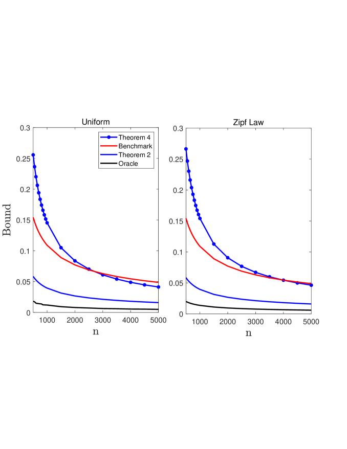
Figure 1: The proposed bounds compared to the benchmark and to an Oracle, as $n$ grows and $\delta=0.05$

Next, we examine the performance of our proposed schemes for a decaying confidence level, $\delta=1/n^{2}$. As above, we set $A=100$ and focus on the two benchmark distributions. Figure 2 demonstrates the results we achieve. Here, we see the advantage of Theorem 4, as it outperforms the alternatives for relatively large $n$. Once again, all bounds attain the prescribed confidence level.

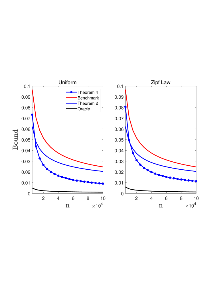
Figure 2: The proposed bounds compared to the benchmark and to an Oracle, as $n$ grows and $\delta=1/n^{2}$

6 Application to Inference of Frequent Events

We now introduce an important application of our proposed scheme. Consider a survey asking individuals for their favorite food. We would like to report the $k$ most popular foods along with their associated CIs. The common approach is to construct $k$ marginal (binomial) intervals of confidence level $1-\delta$ each. This approach is genuinely wrong. For example, consider the case of $k=1$, $n=100$ and a uniform distribution over an alphabet size $A=||p||_{0}$. By definition, the most popular food in the sample would attain at least a single vote. Therefore, its exact lower bound CI (of level $1-\delta=0.95$) is at least $\theta_{l}=2.5\cdot 10^{-4}$. This means that for $A>4000$, we attain zero coverage rate (!). This phenomenon is not quite surprising. Traditional (frequentist) inference assumes a fixed and unknown parameter $\theta$. Here, the inferred parameter is data-dependent, as it corresponds to the most frequent symbols in the sample. That is, we may obtain different $k$ most popular foods for different samples. This type of inference problem is known as selective inference (Ben-Hamou et al., 2017). Selective inference is a complicated task which is extensively studied in recent years (Tibshirani et al., 2016; Berk et al., 2013; Painsky, 2024). One of the first major contributions to the problem is due to Benjamini and Yekutieli (2005). In their work, they showed that conditional coverage, following any selection rule for any set of (unknown) values for the parameters, is impossible to achieve. This means we cannot simply infer on the chosen parameters, given that they were selected.

Naturally, by controlling the infinity norm we implicitly control of the $k$ most frequent events. That is, assume we found $T_{\delta}(X^{n})$ that satisfies (4). Then, we have $|p_{i}-\hat{p}_{i}(X^{n})|\geq T_{\delta}(X^{n})$ for every $i\in\mathbb{N}$ with probability $1-\delta$, including the $k$ most frequent events, $\hat{p}_{[i]},i=1,...,k$. However, it is of a natural concern that such an approach is not tight enough, as it is oblivious to $k$. In the following we study this claim and discuss the tightness of the infinity norm with respect to the $k$ most frequent events.

Theorem 8.

Let $p=p_{i\in\mathbb{N}}$ be a distribution over $\mathbb{N}$. Let $\hat{p}$ be the MLE of $p$. Let $j=\text{argmax}\;\hat{p}_{i}$ be the most frequent symbol in the sample. Assume there exists $U_{\delta}(X^{n})$ such that

$$\mathbb{P}\left(|p_{j}-\hat{p}_{j}|\geq U_{\delta}(X^{n})\right)\leq\delta.$$ (21)

Then,

$$\mathbb{E}(U_{\delta}(X^{n}))\geq z_{\delta/2}\sqrt{\frac{p_{[1]}(1-p_{[1]})}{n}}+O\left(\frac{1}{n}\right)$$ (22)

for sufficiently large $n$.

The proof of Theorem 8 is provided in Section 8.8. It utilizes the optimally of the CP CI and additional asymptotic properties. Let us now consider the $k$ most frequent events. We would like to refrain from multiplicity corrections, so we seek an interval for $\sup_{i\in\mathcal{X}_{k}(X^{n})}|p_{i}-\hat{p}_{i}(X^{n})|$ where $\mathcal{X}_{k}(X^{n})$ is the collection of the $k$ most frequent events in the sample. This set naturally contains the single most frequent event, so a CI of average length (22) is inevitable.

Let us compare Theorem 8 with our proposed bounds. For this purpose we turn to real-world data sets. Notice that in the real-world settings, the true underlying probability is unknown. Hence, we treat the empirical distribution of the full data-set as the underlying distribution and sample from it accordingly. We begin with a census data; we consider the $2000$ United States Census (Bureau, 2014), which lists the frequency of the top $1000$ most common last names in the United States. We randomly sample $n$ names (with replacement) and examine the studied bounds for $\delta=0.05$. In addition, we present the Oracle CIs for the single most frequent symbol and the infinity norm. The left chart of Figure 3 demonstrates the results we achieve. As we can see, the Oracle CIs are very close to each other and the difference between them and Theorem 8 is also negligible. This shows that the infinity norm is a very good proxy to the $k$ most frequent symbols in the alphabet. As we further examine our results, we see that for a typical experiment of $n=10000$, the top $k=5$ surnames are Smith, Johnson, Williams, Brown and Jones with $\hat{p}_{i}=[0.0213,0.0165,0.0137,0.0134,0.0130]$ respectively. Theorem 2 attains a bound of $0.0108$ while the benchmark is about three times greater, $0.0345$. Next, we consider a corpus linguistic experiment. The popular Broadway play Hamilton consists of $20{,}520$ words, of which $3{,}578$ are distinct. We randomly sample $n$ words (with replacement), and evaluate the corresponding bounds. The right chart of Figure 3 demonstrates the results we achieve. Once again,it is quite evident that Theorem 2 outperforms its alternatives in this fixed $\delta=0.05$ regime. Further, we observe that the the infinity norm is a tight proxy to the $k$ most frequent symbols in the alphabet.

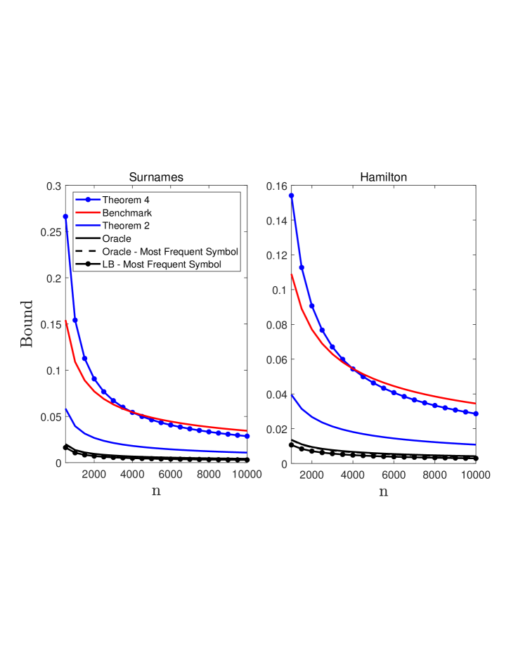
Figure 3: The proposed bounds compared to the benchmark and to an Oracle, as $n$ grows. The lower bound for the most frequent symbol corresponds to Theorem 8

7 Discussion and Conclusions

In this work we study distribution estimation under the $\ell_{\infty}$ norm. We introduce two data-dependent upper bounds for the MLE, which significantly improve upon currently known results. Our first bound (Theorem 2) demonstrates favorable performance in small sample size and fixed $\delta$ regimes. However, its dependency in the data is somewhat involved, compared to our “dream” result (3). Our second bound (Theorem 4) improves the explicit dependency in the data, and demonstrates favorable performance in larger sample regimes, where $\delta$ decays with $n$. The above upper bounds are matched by nearly-optimal lower bounds, demonstrating the tightness of our analysis. Finally, we introduce an important application to our work in selective inference. We show that by utilizing $\ell_{\infty}$ results, we provide relatively tight confidence interval for the most frequent events in the sample.

8 Proofs

8.1 A Proof for Theorem 1

First, notice we have

$$\mathbb{E}\big{(}\sup_{i}|p_{i}-\hat{p}_{i}(X^{n})|\big{)}^{m}\overset{(\text{i})}{=} \mathbb{E}\left(\sup_{i}(p_{i}-\hat{p}_{i}(X^{n}))^{m}\right)\overset{(\text{ii})}{\leq}\mathbb{E}\left(\sum_{i}(p_{i}-\hat{p}_{i}(X^{n}))^{m}\right)=$$

$$\frac{1}{n^{m}}\sum_{i}\mathbb{E}(n_{i}-np_{i})^{m}\overset{(\text{iii})}{\leq}\frac{1}{n^{m}}\sum_{i}\sum_{k=1}^{d}k^{m-k}(np_{i}(1-p_{i}))^{k}$$

where $d=n/2$ and

1. follows from the monotonicity of the power function.

2. The supremum of non-negative elements is bounded from above by their sum (Maddox, 1988).

3. follows from Theorem $4$ of Skorski (2020)

Applying Markov’s inequality we obtain

$$\mathbb{P}\big{(}\sup_{i}|p_{i}-\hat{p}_{i}(X^{n})|\geq a\big{)}\leq \frac{1}{a^{m}}\mathbb{E}\left(\sup_{i}|p_{i}-\hat{p}_{i}(X^{n})|\right)^{m}\leq$$ (23)

$$\frac{1}{a^{m}}\frac{1}{n^{m}}\sum_{i}\sum_{k=1}^{d}k^{m-k}(np_{i}(1-p_{i}))^{k}.$$

Setting the right hand side to equal $\delta$ yields

$$a=\frac{1}{n}\left(\frac{1}{\delta_{1}}\sum_{i}\sum_{k=1}^{d}k^{m-k}(np_{i}(1-p_{i}))^{k}\right)^{1/m}.$$

Therefore, with probability $1-\delta$, we have

$$\sup_{i}|p_{i}-\hat{p}_{i} (X^{n})|\leq\frac{1}{n}\left(\frac{1}{\delta}\sum_{k=1}^{d}k^{m-k}n^{k}\sum_{i}p_{i}^{k}(1-p_{i})^{k}\right)^{1/m}.$$ (24)

Let us further bound from above the right hand side of (24). We have,

$$\sum_{i}p_{i}^{k}(1-p_{i})^{k}\overset{(\text{i})}{\leq} \max_{t\in[0,1]}t^{k-1}(1-t)^{k}\overset{(\text{ii})}{\leq}\left(\frac{k-1}{2k-1}\right)^{k-1}\left(\frac{k}{2k-1}\right)^{k}\overset{(\text{iii})}{\leq}$$ (25)

$$\left(\frac{k}{2k-1}\right)^{2k-1}=\left(1+\frac{-k+1}{2k-1}\right)^{2k-1}\overset{(\text{iv})}{\leq}\exp(-k+1)$$

1. follows from $\sum_{i}p_{i}\psi(p_{i})\leq\max_{t\in[0,1]}\psi(t)$ for $\psi(p_{i})=p_{i}^{k-1}(1-p_{i})^{k}$. That is, the mean of a random variable not greater than its maximum.

2. simple derivation shows that the maximum of $t^{k-1}(1-t)^{k}$ is attained for $t^{*}=\frac{k-1}{2k-1}$.

3. is due to $\left(\frac{k-1}{2k-1}\right)^{k-1}\leq\left(\frac{k}{2k-1}\right)^{k-1}$.

4. follows from Bernoulli inequality.

Importantly, notice that for a choice of $p=[1/2,1/2,0,\dots,0]$ we have

$$\sum_{i}p_{i}^{k}(1-p_{i})^{k}=2\left(\frac{1}{2}\right)^{2k}=\left(\frac{1}{2}\right)^{2k-1},$$ (26)

which approaches the term on the right hand side of inequality (iii), as $k$ increases. Finally, plugging (25) to (24) we obtain

$$\sup_{i}|p_{i}-\hat{p}_{i}(X^{n})|\leq \frac{1}{n}\left(\frac{1}{\delta}\sum_{k=1}^{d}k^{m-k}n^{k}\exp(-k+1)\right)^{1/m}=$$ (27)

$$\frac{1}{\sqrt{n}}\left(\frac{\sqrt{m/2}}{\delta^{1/m}}\right)\exp\left(-\frac{1}{2}+\frac{1}{m}\right)+O\left(\frac{1}{n^{\frac{1}{2}+\frac{1}{m}}}\right)$$

for every even $m>0$.

8.2 A Proof for Theorem 2

We begin with the following proposition.

Proposition 9.

Let $\delta_{2}>0$. Then, with probability $1-\delta_{2}$,

$$\sum_{i}\sum_{k=1}^{m/2}k^{m-k}( np_{i}(1-p_{i}))^{k}\leq\frac{n}{n-1}\bigg{(}\sum_{i}\sum_{k=1}^{m/2}k^{m-k}(n\hat{p}_{i}(1-\hat{p}_{i}))^{k}+\epsilon\bigg{)}$$ (28)

for every even $m$, where

$$\epsilon=\sqrt{\frac{n}{2}\log(1/\delta_{2})}\sum_{k=1}^{d} k^{m-k}n^{k}\bigg{(}\frac{k}{n4^{k-1}}+\frac{3k(k-1)(k-2)}{n^{3}\cdot 2^{2k-5}}\bigg{)}.$$ (29)

Proof.

Define $\psi(n,d,\hat{p})=\sum_{i}\sum_{k=1}^{d}k^{m-k}(n\hat{p}_{i}(1-\hat{p}_{i}))^{k}$. McDiarmind’s inequality suggests that

$$\text{P}\left(\psi(n,d,\hat{p})-\mathbb{E}\left(\psi(n,d,\hat{p})\right)\leq-\epsilon\right)\leq\exp\left(\frac{-2\epsilon^{2}}{\sum_{j=1}^{n}c_{j}^{2}}\right)$$

where

$$\sup_{x^{\prime}_{j}\in\mathcal{X}}\big{|}\psi(n,d,\hat{p})-\psi(n,d,\hat{p}^{\prime})\big{|}\leq c_{j}.$$ (30)

where $\hat{p}^{\prime}$ is the MLE over the same sample $x^{n}$, but with a different $j^{th}$ observation, $x_{j}^{\prime}$. First, let us find $c_{j}$. We have

$$\sup_{x^{\prime}_{j}\in\mathcal{X}}\big{|}\psi(n,d,\hat{p})-\psi(n,d,\hat{p}^{\prime})\big{|}\overset{(\text{i})}{\leq}$$ (31)

$$\sup_{p\in[0,1-1/n]}2\big{|}\sum_{k=1}^{d}k^{m-k}\left(np(1-p)\right)^{k}-\sum_{k=1}^{d}k^{m-k}\left(n(p+1/n)(1-(p+1/n))\right)^{k})\big{|}=$$

$$\sup_{p\in[0,1-1/n]}2\big{|}\sum_{k=1}^{d}k^{m-k}n^{k}\left(p(1-p)\right)^{k}-\left((p+1/n)(1-(p+1/n))\right)^{k})\big{|}\overset{(\text{ii})}{\leq}$$

$$2\sum_{k=1}^{d}k^{m-k}n^{k}\left(\frac{k}{n\cdot 4^{k-1}}+\frac{3k(k-1)(k-2)}{n^{3}\cdot 2^{2k-5}}\right)$$

where

1. Changing a single observation effects only two symbols (for example, $\hat{p}_{l}$ and $\hat{p}_{t}$), where the change is $\pm 1/n$.

2. Please refer to Appendix A below.

Next, we have

$$\mathbb{E}(\psi(n,d,\hat{p}))\geq \sum_{i}\sum_{k=1}^{d}k^{m-k}n^{k}\left(\mathbb{E}(\hat{p}_{i}(1-\hat{p}_{i}))\right)^{k}=$$

$$\sum_{i}\sum_{k=1}^{d}k^{m-k}n^{k}\left(\left(1-\frac{1}{n}\right)p_{i}(1-p_{i})\right)^{k}\geq$$

$$\left(1-\frac{1}{n}\right)\sum_{i}\sum_{k=1}^{d}k^{m-k}(np_{i}(1-p_{i}))^{k}$$ (32)

where the first inequality follows from Jensen Inequality and the equality that follows is due to $\mathbb{E}(\hat{p}_{i}(1-\hat{p}_{i}))=p(1-p)(1-1/n)$. Going back to McDiarmind’s inequality, we have

$$\mathbb{P}\left(\mathbb{E}\psi(n,d,\hat{p})\geq\psi(n,d,\hat{p})+\epsilon\right)\leq\exp\left(\frac{-2\epsilon^{2}}{nc_{j}^{2}}\right)$$ (33)

In word, the probability that the random variable $Z=\psi(n,d,\hat{p})$ is smaller than a constant $C=\mathbb{E}(\psi(n,d,\hat{p}))-\epsilon$ is not greater that $\nu=\exp\left(-2\epsilon^{2}/{\sum_{j=1}^{n}c_{j}^{2}}\right)$. Therefore, it necessarily means that the probability that $Z$ is smaller than a constant smaller than $C$, is also not greater than $\nu$. Hence, plugging (32) we obtain

$$\mathbb{P}\left(\left(1-\frac{1}{n}\right)\psi(n,d,p)\geq\psi(n,d,\hat{p})+\epsilon\right)\leq\exp\left(\frac{-2\epsilon^{2}}{\sum_{j}c_{j}^{2}}\right)$$

Setting the right hand side to equal $\delta_{2}$ we get

$$\epsilon=\sqrt{\frac{n}{2}\log(1/\delta_{2})}\sum_{k=1}^{d} k^{m-k}n^{k}\left(\frac{k}{n\cdot 4^{k-1}}+\frac{3k(k-1)(k-2)}{n^{3}\cdot 2^{2k-5}}\right)$$ (34)

and with probability $1-\delta_{2}$,

$$\sum_{i}\sum_{k=1}^{d}k^{m-k} (np_{i}(1-p_{i}))^{k}\leq\frac{n}{n-1}\left(\sum_{i}\sum_{k=1}^{d}k^{m-k}(n\hat{p}_{i}(1-\hat{p}_{i}))^{k}+\epsilon\right)$$ (35)

∎

Finally, we apply the union bound to (24) with $\delta=\delta_{1}$ and Proposition 9 to obtain the stated result.

8.2.1 A Proof for Corollary 2.1

We prove the Corollary with two propositions.

Proposition 10.

Let $\delta_{1}>0$. Then, with probability $1-\delta_{1}$,

$$\sup_{i\in\mathcal{X}}|p_{i}-\hat{p}_{i}(X^{n})|\leq\frac{m}{2n}\left(\frac{1}{\delta_{1}}\right)^{1/m}\left(\sum_{i}\sum_{k=1}^{m/2}(np_{i}(1-p_{i}))^{k}\right)^{1/m}$$ (36)

for every even $m>0$.

Proof.

First, we have

$$\mathbb{E}\big{(}\sup_{i}|p_{i}-\hat{p}_{i}(X^{n})|\big{)}^{m}\overset{(\text{i})}{\leq} \frac{1}{n^{m}}\sum_{i}\sum_{k=1}^{d}k^{m-k}(np_{i}(1-p_{i}))^{k}\overset{(\text{ii})}{\leq}$$

$$\left(\frac{d}{m}\right)^{m}\sum_{i}\sum_{k=1}^{d}(np_{i}(1-p_{i}))^{k}$$

where $d=n/2$ and

1. follows from (15) in the main text .

2. follows from $k^{m-k}\leq d^{m}$ for every $k\in\{1,...,d\}$.

Applying Markov’s inequality we obtain

$$\mathbb{P}\left(\sup_{i}|p_{i}-\hat{p}_{i}(X^{n})|\geq a\right)\leq \frac{1}{a^{m}}\mathbb{E}\left(\sup_{i}|p_{i}-\hat{p}_{i}(X^{n})|\right)^{m}\leq$$ (37)

$$\frac{1}{a^{m}}\left(\frac{d}{n}\right)^{m}\sum_{i}\sum_{k=1}^{d}(np_{i}(1-p_{i}))^{k}.$$

Setting the right hand side to equal $\delta_{1}$ yields

$$a=\left(\frac{1}{\delta_{1}}\left(\frac{d}{n}\right)^{m}\sum_{i}\sum_{k=1}^{d}(np_{i}(1-p_{i}))^{k}\right)^{1/m}=\frac{m}{2n}\left(\frac{1}{\delta_{1}}\sum_{i}\sum_{k=1}^{m/2}(np_{i}(1-p_{i}))^{k}\right)^{1/m}.$$

∎

Proposition 11.

Let $\delta_{2}>0$. Then, with probability $1-\delta_{2}$,

$$\sum_{i}\sum_{k=1}^{d}(np_{i}(1-p_{i}))^{k}\leq$$ (38)

$$\frac{n}{n-1}\left(\sum_{i}\sum_{k=1}^{d}(n\hat{p}_{i}(1-\hat{p}_{i}))^{k}+d\sqrt{\frac{1}{2}\log(1/\delta_{2})}\left(2n^{d-1/2}+48n^{d-5/2}\right)\right)$$

for every even $m$.

Proof.

McDiarmind’s inequality suggests that

$$\mathbb{P}\left(\sum_{i}\sum_{k=1}^{d}(n\hat{p}_{i}(1-\hat{p}_{i}))^{k}-\mathbb{E}\left(\sum_{i}\sum_{k=1}^{d}(n\hat{p}_{i}(1-\hat{p}_{i}))^{k}\right)\leq-\epsilon\right)\leq\exp\left(\frac{-2\epsilon^{2}}{\sum_{j=1}^{n}c_{j}^{2}}\right)$$

where

$$\sup_{x^{\prime}_{j}\in\mathcal{X}}\big{|}\sum_{i}\sum_{k=1}^{d}\left(n\hat{p}_{i}(1-\hat{p}_{i})\right)^{k}-\sum_{i}\sum_{k=1}^{d}\left(n\hat{p}^{\prime}_{i}(1-\hat{p}^{\prime}_{i})\right)^{k})\big{|}\leq c_{j}.$$ (39)

First, let us find $c_{j}$. We have

$$\sup_{x^{\prime}_{j}\in\mathcal{X}}\big{|}\sum_{i}\sum_{k=1}^{d}\left(n\hat{p}_{i}(1-\hat{p}_{i})\right)^{k}-\sum_{i}\sum_{k=1}^{d}\left(n\hat{p}^{\prime}_{i}(1-\hat{p}^{\prime}_{i})\right)^{k})\big{|}\overset{(\text{i})}{\leq}$$ (40)

$$2\sup_{p\in[0,1-1/n]}\big{|}\sum_{k=1}^{d}\left(np(1-p)\right)^{k}-\sum_{k=1}^{d}\left(n(p+1/n)(1-(p+1/n))\right)^{k})\big{|}=$$

$$2\sup_{p\in[0,1-1/n]}\big{|}\sum_{k=1}^{d}n^{k}\left(p(1-p)\right)^{k}-\left((p+1/n)(1-(p+1/n))\right)^{k})\big{|}\leq$$

$$2\sum_{k=1}^{d}n^{k}\sup_{p\in[0,1-1/n]}\big{|}\left(p(1-p)\right)^{k}-\left((p+1/n)(1-(p+1/n))\right)^{k})\big{|}\overset{(\text{ii})}{=}$$

$$2\sum_{k=1}^{d}n^{k}\left(\frac{k}{n\cdot 4^{k-1}}+\frac{3k(k-1)(k-2)}{n^{3}\cdot 2^{2k-5}}\right)\leq$$

$$n^{d-1}\sum_{k=1}^{d}\left(\frac{2k}{4^{k-1}}+\frac{3k(k-1)(k-2)}{n^{2}\cdot 2^{2k-4}}\right)\overset{(\text{iii})}{\leq}2dn^{d-1}+48dn^{d-3}$$

where

1. Changing a single observation effects only two symbols (for example, $\hat{p}_{l}$ and $\hat{p}_{t}$), where the change is $\pm 1/n$.

2. Please refer to Appendix A.

3. Follows from $\sum_{k=1}^{d}\frac{k}{4^{k-1}}=4\sum_{k=1}^{d}\frac{k}{4^{k}}\leq d$ and

   $$\sum_{k=1}^{d}\frac{k(k-1)(k-2)}{4^{k-2}}\leq\sum_{k=1}^{d}\frac{k^{3}}{4^{k-2}}\leq d\max_{k\in[1,d]}\frac{k^{3}}{4^{k-2}}\leq 16\frac{2\exp(-3)}{\log(4)}\leq 16$$ (41)

   where the maximum is obtain for $k^{*}=3/\log(4)$.

next, we have

$$\mathbb{E}\bigg{(}\sum_{i}\sum_{k=1}^{d} (n\hat{p}_{i}(1-\hat{p}_{i}))^{k}\bigg{)}\geq\sum_{i}\sum_{k=1}^{d}\left(\mathbb{E}(n\hat{p}_{i}(1-\hat{p}_{i}))\right)^{k}=$$ (42)

$$\sum_{i}\sum_{k=1}^{d}n^{k}\left(\left(1-\frac{1}{n}\right)p_{i}(1-p_{i})\right)^{k}\geq\left(1-\frac{1}{n}\right)\sum_{i}\sum_{k=1}^{d}(np_{i}(1-p_{i}))^{k}$$

Going back to McDiarmind’s inequality, we have

$$\mathbb{P}\left(\mathbb{E}\left(\sum_{i}\sum_{k=1}^{d}(n\hat{p}_{i}(1-\hat{p}_{i}))^{k}\right)\geq\sum_{i}\sum_{k=1}^{d}(n\hat{p}_{i}(1-\hat{p}_{i}))^{k}+\epsilon\right)\leq\exp\left(\frac{-2\epsilon^{2}}{\sum_{j=1}^{n}c_{j}^{2}}\right)$$ (43)

Plugging (42) we obtain

$$\mathbb{P}\left(\left(1-\frac{1}{n}\right)\sum_{i}\sum_{k=1}^{d}(np_{i}(1-p_{i}))^{k}\geq\sum_{i}\sum_{k=1}^{d}(n\hat{p}_{i}(1-\hat{p}_{i}))^{k}+\epsilon\right)\leq\exp\left(\frac{-2\epsilon^{2}}{\sum_{j}c_{j}^{2}}\right)$$

Setting the right hand side to equal $\delta_{2}$ we get

$$\epsilon=\sqrt{\frac{n}{2}\log(1/\delta_{2})}\left(2dn^{d-1}+48dn^{d-3}\right)$$

and with probability $1-\delta_{2}$,

$$\sum_{i}\sum_{k=1}^{d}(np_{i}(1-p_{i}))^{k}\leq$$ (44)

$$\frac{n}{n-1}\left(\sum_{i}\sum_{k=1}^{d}(n\hat{p}_{i}(1-\hat{p}_{i}))^{k}+d\sqrt{\frac{1}{2}\log(1/\delta_{2})}\left(2n^{d-1/2}+48n^{d-5/2}\right)\right)$$

∎

Finally, we apply the union bound to Propositions 10 and 11 to obtain

$$\sup_{i\in\mathcal{X}}|p_{i}-\hat{p}_{i}(X^{n})|\leq$$

$$\frac{m}{2n}\left(\frac{1}{\delta_{1}}\frac{n}{n-1}\left(\sum_{i}\sum_{k=1}^{d}(n\hat{p}_{i}(1-\hat{p}_{i}))^{k}+d\sqrt{\frac{1}{2}\log(1/\delta_{2})}\left(2n^{d-1/2}+48n^{d-5/2}\right)\right)\right)^{1/m}\leq$$

$$\frac{m}{2\delta_{1}^{1/m}}\frac{1}{n}\left(\frac{n}{n-1}\right)^{1/m}\left(\sum_{i}\sum_{k=1}^{m/2}(n\hat{p}_{i}(1-\hat{p}_{i}))^{k}\right)^{1/m}+$$

$$\frac{m}{2\delta_{1}^{1/m}}\frac{1}{n}\left(\frac{n}{n-1}\right)^{1/m}(m/2)^{1/m}\left(\frac{1}{2}\log\left(\frac{1}{\delta_{2}}\right)\right)^{1/m}\left(2n^{\frac{1}{2}-\frac{1}{2m}}+48n^{\frac{1}{2}-\frac{5}{2m}}\right)$$

with probability $1-\delta_{1}-\delta_{2}$. Define $g(m,\delta_{1})={m}/{\delta_{1}^{1/m}}$. Further, it is immediate to show that $(m/2)^{1/m}\leq\sqrt{\exp(1/\exp(1))}$. Hence, with probability $1-\delta_{1}-\delta_{2}$,

$$\sup_{i\in\mathcal{X}}|p_{i}-\hat{p}_{i}(X^{n})|\leq \frac{g(m,\delta_{1})}{n}\left(\sum_{i}\sum_{k=1}^{m/2}(n\hat{p}_{i}(1-\hat{p}_{i}))^{k}\right)^{1/m}+$$

$$bg(m,\delta_{1})(\log(1/\delta_{2}))^{1/2m}\left(n^{-\frac{1}{2}\left(1+\frac{1}{m}\right)}+24n^{-\frac{1}{2}\left(1+\frac{5}{m}\right)}\right)$$

for every even $m$, where $b=\sqrt{2\exp(1/\exp(1))}$. Finally, we would like to choose $m$ which minimizes $g(m,\delta_{1})$. We show in Appendix B that $\inf_{m}g(m,\delta_{1})=\exp(1)\log(1/\delta_{1})$, where and the infimum is obtained for a choice of $m^{*}=\log(1/\delta_{1})$.

8.3 A Proof of Theorem 3

Let us first introduce some auxiliary results and background

8.3.1 Auxiliary Results

Lemma 12 (contained in the proof of Lemma 10, Cohen and Kontorovich (2023)).

Let $Y_{i\in I\subseteq\mathbb{N}}$ be random variables such that, for each $i\in I$, there are $v_{i}>0$ and $a_{i}\geq 0$ satisfying

$$\mathop{\mathbb{P}}\left(Y_{i}\geq\varepsilon\right) \leq \exp\left(-\frac{\varepsilon^{2}}{2(v_{i}+a_{i}\varepsilon)}\right),\qquad\varepsilon\geq 0.$$ (45)

Put

$$\begin{array}[]{l}v^{*}:=\sup_{i\in I}v_{i},\quad V^{*}:=\sup_{i\in I}v_{i}\log(i+1),\quad a^{*}:=\sup_{i\in I}a_{i},\quad A^{*}:=\sup_{i\in I}a_{i}\log(i+1).\end{array}$$ (47)

Then

$$\mathop{\mathbb{P}}\left(\sup_{i\in I}Y_{i}\geq 2\sqrt{V^{*}+v^{*}\log\frac{1}{\delta}}+4A^{*}+4a^{*}\log\frac{1}{\delta}\right) \leq \delta.$$

Remark 8.1.

When considering the random variable $Z=\sup_{i\in\mathbb{N}}|\hat{p}_{i}-p_{i}|$, there is no loss of generality in assuming that $p_{i}\leq 1/2$, $i\in\mathbb{N}$. Indeed, $|Y_{i}|=|\hat{p}_{i}-p_{i}|$ is distributed as $|n^{-1}\operatorname{Bin}(n,p_{i})-p_{i}|$, and the latter distribution is invariant under the transformation $p_{i}\mapsto 1-p_{i}$.

Lemma 13.

For any distribution $p_{i\in\mathbb{N}}$,

$$V(p) \leq \varphi(v^{*}(p)).$$

Proof.

(This elegant proof idea is due to Václav Voráček.) There is no loss of generality in assuming $p=p^{\downarrow}$. The claim then amounts to

$$\sup_{i\in\mathbb{N}}v_{i}\log(i+1)\leq v^{*}\log\frac{1}{v^{*}}.$$

The monotonicity of the $p_{i}$ implies $p_{i}\leq(p_{1}+\ldots+p_{i})/i\leq 1/i$. Now $x\leq 1/i\implies x(1-x)\leq 1/(i+1)$ for $i\in\mathbb{N}$, and hence $v_{i}\leq 1/(i+1)$. Thus, $v_{i}\log(i+1)\leq v_{i}\log\frac{1}{v_{i}}$. Finally, since $x\log(1/x)$ is increasing on $[0,1/4]$, which is the range of the $v_{i}$, we have $\sup_{i\in\mathbb{N}}v_{i}\log\frac{1}{v_{i}}\leq v^{*}\log\frac{1}{v^{*}}$. ∎

Remark 8.2.

There is no reverse inequality of the form $\varphi(v^{*}(p))\leq F(V^{*}(p))$, for any fixed $F:\mathbb{R}_{+}\to\mathbb{R}_{+}$. This can be seen by considering $p$ supported on $[k]$, with $p_{1}=\log(k)/k$ and the remaining masses uniform. Then $V^{*}(p)\approx\log(k)/k$ while $\varphi(v^{*}(p))\approx\log(k)\log(k/\log k)/k$.

Proposition 14.

Let $n\geq 10$ and $\beta=\log(n)$. Then,

$$f(n)=\frac{\beta^{-\beta}n^{2}\left(\frac{n-\beta}{n}\right)^{\beta-n}}{2^{\beta}-2}\leq\frac{81}{2}.$$

Proof.

To prove the above, we show that $f(n)$ is decreasing for $n>200$. This means that the maximum of $f(n)$ may be numerically evaluated in the range $n\in\{10,...,200\}$. Finally, we verify that the maximum of $f(n)$ is attained for $n=33$, and is bounded from above by $81/2$ as desired. It remains to verify that $f(n)$ is decreasing for $n>200$. Since $f(n)$ is non-negative, it is enough to show that $g(n)=\log f(n)$ is decreasing. Denote

$$g(n)=-\beta\log\beta+2\log n+(n-\beta)\log(n-\beta)+(n-\beta)\log n-\log(2^{\beta}-2).$$ (48)

Taking the derivative of $g(n)$ we have,

$$g^{\prime}(n)=$$ (49)

$$-\frac{1}{n}(\log\beta+1)+\frac{2}{n}+\left(1-\frac{1}{n}\right)(-\log(n-\beta)-1+\log n)+\frac{n-\beta}{n}-\frac{1}{n}\frac{2^{\beta}\log 2}{2^{\beta}-2}=$$

$$\frac{1}{n}\left((n-1)\log\frac{n}{n-\beta}-\log\beta-\beta+2-\frac{2^{\beta}\log 2}{2^{\beta}-2}\right)\leq$$

$$\frac{1}{n}\left(n\log\frac{n}{n-\beta}-\log\beta-\beta+2-\log 2\right)\leq\frac{1}{n}\left(\frac{n\beta}{n-\beta}-\log\beta-\beta+2-\log 2\right)=$$

$$\frac{1}{n}\left(\frac{\beta^{2}}{n-\beta}-\log\beta+2-\log 2\right),$$

where the first inequality follows from $\log(n/(n-\beta))\geq 1$ and $2^{\beta}/(2^{\beta}-2)\geq 1$, while the second inequality is due to Bernoulli’s inequality, $(n/(n-\beta))^{n}\leq\exp(n\beta/(n-\beta))$. Finally, it is easy to show that $\beta^{2}/(n-\beta)$ is decreasing for $n\geq 10$. This means that $\beta^{2}/(n-\beta)\leq(\log 10)^{2}/(10-\log(10))$ and $g^{\prime}(n)<0$ for $n>200$. ∎

Lemma 15 (generalized Fano method (Yu, 1997), Lemma 3).

For $r\geq 2$, let $\mathcal{M}_{r}$ be a collection of $r$ probability measures $\nu_{1},\nu_{2},...,\nu_{r}$ with some parameter of interest $\theta(\nu)$ taking values in pseudo-metric space $(\Theta,\rho)$ such that for all $j\neq k$, we have

$$\rho(\theta(\nu_{j}),\theta(\nu_{k}))\geq\alpha$$

and

$$D(\nu_{j}~{}\|~{}\nu_{k})\leq\beta.$$

Then

$$\inf_{\hat{\theta}}\max_{j\in[d]}\mathbb{E}_{Z\sim\mu_{j}}\rho(\hat{\theta}(Z),\theta(\nu_{j}))\geq\frac{\alpha}{2}\left(1-\left(\frac{\beta+\log 2}{\log r}\right)\right),$$

where the infimum is over all estimators $\hat{\theta}:Z\mapsto\Theta$.

Proposition 16.

Let $p$ and $q$ be two distributions with support size $n$. Define $p$ by

$$p_{1}=\frac{\log n}{2n\log\log n},\quad p_{i}=\frac{1-p_{1}}{n-1},\qquad i>1,$$

and $q$ by $q_{2}=p_{1}$, and $q_{i}=p_{2}$ for $i\neq 2$. Then,

1. $\left\|p-q\right\|_{\infty}\geq c\frac{\log n}{n\log\log n}$ for some $c>0$ and all $n$ sufficiently large.

2. $\lim_{n\rightarrow\infty}\frac{n}{\log n}D(p||q)=\frac{1}{2}$

Proof.

For the first part, it is enough to show that

$$|p_{1}-p_{2}|\geq c\log(n)/n\log\log n$$

for some $c>0$ and sufficiently large $n$. First, we show that $p_{1}\geq p_{2}$ for $n\geq(\log n)^{2}$. That is,

$$p_{1}-\frac{1-p_{1}}{n-1}=\frac{np_{1}-1}{n-1}>0$$ (50)

for $np_{1}>1$. Next, fix $0<c\leq 1/2$. We have,

$$|p_{1}-p_{2}|-\frac{c\log(n)}{n\log\log n}= \frac{ap_{1}-1}{n-1}-\frac{c\log n}{n\log\log n}=$$ (51)

$$\frac{1}{n-1}\left(\frac{\log n}{2\log\log n}-1-\frac{n-1}{n}\frac{c\log n}{\log\log n}\right)=$$

$$\frac{1}{(n-1)2\log\log n}\left(\log n\left(1-\frac{n-1}{n}2c\right)-2\log\log n\right)>0$$

where the last inequality holds for $c(n-1)/n<1/2$ and sufficiently large $n$, as desired. We now proceed to the second part of the proof.

$$\frac{n}{\log n}D(p||q)=\frac{n}{\log n}\left(p_{1}\log\frac{p_{1}}{q_{1}}+p_{2}\log\frac{p_{2}}{q_{2}}\right)=\frac{n}{\log n}(p_{1}-p_{2})\log\frac{p_{1}}{p_{2}}.$$ (52)

First, we have

$$\frac{n}{\log n}(p_{1}-p_{2})= \frac{n}{\log n}\left(p_{1}-\frac{1-p_{1}}{n-1}\right)=\frac{n}{\log n}\left(\frac{np_{1}-1}{n-1}\right)=$$ (53)

$$\frac{n}{\log n}\frac{\log n/2n\log\log n-1}{n-1}=\frac{n}{n-1}\left(\frac{1}{2\log\log n}-\frac{1}{\log n}\right).$$

Next,

$$\log\frac{p_{1}}{p_{2}}= \log(n-1)+\log\frac{p_{1}}{1-p_{1}}=\log(n-1)+\log\frac{\log n}{2n\log\log n-\log n}=$$ (54)

$$\log(n-1)+\log\log n-2\log(2n\log\log n-\log n).$$

Putting it all together we obtain

$$\frac{n}{\log n} D(p||q)=$$ (55)

$$\frac{n}{n-1}\left(\frac{1}{2\log\log n}-\frac{1}{\log n}\right)\left(\log(n-1)+\log\log n-2\log(2n\log\log n-\log n)\right)=$$

$$\frac{n}{n-1}\bigg{(}\frac{\log(n-1)}{2\log\log n}-\frac{\log(n-1)}{\log n}+\frac{1}{2}-\frac{\log\log n}{\log n}-$$

$$\quad\quad\quad\;\;\frac{\log(2n\log\log n-\log n)}{2\log\log n}+\frac{\log(2n\log\log n-\log n)}{\log n}\bigg{)}=$$

$$\frac{n}{n-1}\bigg{(}\frac{1}{2}+\frac{\log(n-1)-\log(2n\log\log n-\log n)}{2\log\log n}+$$

$$\quad\quad\quad\;\;\frac{\log(2n\log\log n-\log n)-\log(n-1)}{\log n}-\frac{\log\log n}{\log n}\bigg{)}.$$

It is straightforward to show that the last three terms in the parenthesis above converge to zero for sufficiently large $n$, which leads to the stated result. ∎

Lemma 17 (Peres (2017)).

When estimating a single Bernoulli parameter in the range $[0,p_{0}]$, $\Theta(p_{0}\varepsilon^{-2}\log(1/\delta))$ draws are both necessary and sufficient to achieve additive accuracy $\varepsilon$ with probability at least $1-\delta$.

Bernstein inequalities
Background: Let $Y\sim\text{Bin}(n,\theta)$ be a Binomial random variable and let $\hat{\theta}=Y/n$ be the its MLE.

• Classic Bernstein (Boucheron et al., 2003):

  $$\mathop{\mathbb{P}}\left(\hat{\theta}-\theta\geq\varepsilon\right) \leq \exp\left(-\frac{n\varepsilon^{2}}{2(\theta(1-\theta)+\varepsilon/3}\right)$$ (56)

  with an analogous bound for the left tail. This implies:

  $$|\theta-\hat{\theta}| \leq \sqrt{\frac{2\theta(1-\theta)}{n}\log\frac{2}{\delta}}+\frac{2}{3n}\log\frac{2}{\delta}.$$ (57)

• Empirical Bernstein (Dasgupta and Hsu, 2008a, Lemma 5):

  $$|\theta-\hat{\theta}| \leq \sqrt{\frac{5\hat{\theta}(1-\hat{\theta})}{n}\log\frac{2}{\delta}}+\frac{5}{n}\log\frac{2}{\delta}.$$ (58)

We are now ready to present the proof of Theorem $3$.

8.3.2 Proof of Theorem 3

We assume without loss of generality that $p$ is sorted in descending order: $p_{1}\geq p_{2}\geq\ldots$ and further, as per Remark 8.1, that $p_{1}\leq 1/2$. The estimate $\hat{p}_{i}$ is just the MLE based on $n$ iid draws.

Our strategy for analyzing $\sup_{i\in\mathbb{N}}\left\lvert{\hat{p}_{i}-p_{i}}\right\rvert$ will be to break up $p$ into the “heavy” masses, where we apply a maximal Bernstein-type inequality, and the “light” masses, where we apply a multiplicative Chernoff-type bound.

We define the “heavy” masses as those with $p_{i}\geq 1/n$. Denote by $I\subset\mathbb{N}$ the set of corresponding indices and note that $|I|\leq n$. For $i\in I$, put $Y_{i}=\hat{p}_{i}-p_{i}$. Then (56) implies that each $Y_{i}$ satisfies (45) with $v_{i}=p_{i}(1-p_{i})/n$ and $a_{i}=1/(3n)$; trivially, $\max_{i\in I}a_{i}\log(i+1)=\log(n+1)/(3n)$. Invoking Lemma 12 twice (once for $Y_{i}$ and again for $-Y_{i}$) together with the union bound,

we have, with probability $\geq 1-\delta$,

$$\max_{i\in I}|\hat{p}_{i}-p_{i}|\leq 2\sqrt{\frac{V^{*}}{n}+\frac{v^{*}}{n}\log\frac{2}{\delta}}+\frac{4\log(n+1)}{3n}+\frac{4}{3n}\log\frac{2}{\delta}.$$ (59)

Next, we analyze the light masses. Our first “segment” consisted of the $p_{i}\in[n^{-1},1]$; these were the heavy masses. We take the next segment to consist of $p_{i}\in[(2n)^{-1},n^{-1}]$, of which there are at most $2n$ atoms. The segment after that will be in the range $[(4n)^{-1},(2n)^{-1}]$, and, in general, the $k$th segment is in the range $[(2^{k}n)^{-1},(2^{k-1}n)^{-1}]$, and will contain at most $2^{k}n$ atoms. To the $k$th segment, we apply the Chernoff bound $\mathbb{P}(\hat{p}\geq p+\varepsilon)\leq\exp(-nD(p+\varepsilon||p))$, where $p=(2^{k}n)^{-1}$ and $\varepsilon=\varepsilon_{k}=2^{k}p\beta-p$, for some $\beta$ to be specified below. [Note that $D(\alpha p||p)$ is monotonically increasing in $p$ for fixed $\alpha$, so we are justified in taking the left endpoint.] For this choice, in the $k$th segment we have

$$D(p+\varepsilon||p) = D(2^{k}p\beta||p)=D\left(\frac{\beta}{n}\Big{\|}\frac{1}{2^{k}n}\right)$$

$$= \frac{(n-\beta)\log\left(\frac{2^{k}(n-\beta)}{2^{k}n-1}\right)+\beta\log\left(2^{k}\beta\right)}{n}$$

$$\geq \frac{(n-\beta)\log\left(\frac{n-\beta}{n}\right)+\beta\log\left(2^{k}\beta\right)}{n},$$

since neglecting the $-1/2^{k}$ additive term in the denominator decreases the expression. Let $E$ be the event that any of the $p_{i}$s in any of the segments $k=1,2,\ldots$ has a corresponding $\hat{p}_{i}$ that exceeds $\beta/n$. Then

$$\mathbb{P}(E) \leq \sum_{k=1}^{\infty}2^{k}n\exp\left(-(n-\beta)\log\left(\frac{n-\beta}{n}\right)-\beta\log\left(2^{k}\beta\right)\right)=\frac{2\beta^{-\beta}n\left(\frac{n-\beta}{n}\right)^{\beta-n}}{2^{\beta}-2}.$$

For the choice $\beta=\log n$, we have

$$\mathbb{P}(E)\leq\frac{2\beta^{-\beta}n\left(\frac{n-\beta}{n}\right)^{\beta-n}}{2^{\beta}-2} \leq \frac{81}{n},\qquad n\geq 10,$$ (60)

which is proved in Proposition 14. Now $E$ is the event that $\sup_{i:p_{i}<1/n}(\hat{p}_{i}-p_{i})\geq\log(n)/n$. Since $p_{i}<1/n$, there is no need to consider the left-tail deviation at this scale, as all of the probabilities will be zero. Combining (59) with (60) yields (16). Since Lemma  13 implies that $V^{*}\leq\varphi(v^{*})$, (17) follows from (16). Finally, (18) follows from (16) via the obvious relation $V^{*}\leq\log(n+1)v^{*}$.

8.4 A Proof for Theorem 4

We begin with an elementary observation: for $N\in\mathbb{N}$ and $a,b\in[0,1]^{N}$, we have

$$\left\lvert{\max_{i\in[N]}a_{i}(1-a_{i})-\max_{i\in[N]}b_{i}(1-b_{i})}\right\rvert \leq \max_{i\in[N]}\left\lvert{a_{i}-b_{i}}\right\rvert,$$

and this also carries over to $a,b\in[0,1]^{\mathbb{N}}$. Let us denote $v^{*}:=\sup_{i\in\mathbb{N}}p_{i}(1-p_{i})$ and $\hat{v}^{*}:=\sup_{i\in\mathbb{N}}\hat{p}_{i}(1-\hat{p}_{i})$. Together with (18), this implies

$$\left\lvert{v^{*}-\hat{v}^{*}}\right\rvert\leq\left\|p-\hat{p}\right\|_{\infty}\leq a+b\sqrt{v^{*}}$$

where

$$a = \frac{4}{3n}\log\frac{2(n+1)}{\delta}+\frac{\log n}{n},$$

$$b = 2\sqrt{\frac{\log(n+1)}{n}+\frac{1}{n}\log\frac{2}{\delta}}.$$

Following the proof of Lemma $5$ in Dasgupta and Hsu (2008a),

$$|v^{*}-\hat{v}^{*}| \leq a+b\sqrt{v^{*}}$$

$$\leq a+b\sqrt{\hat{v}^{*}+|v^{*}-\hat{v}^{*}|}$$

$$\leq a+b\sqrt{\hat{v}^{*}}+b\sqrt{|v^{*}-\hat{v}^{*}|},$$

where we used $v^{*}\leq\hat{v}^{*}+|v^{*}-\hat{v}^{*}|$ and $\sqrt{x+y}\leq\sqrt{x}+\sqrt{y}$. Now we have an expression of the form

$$A\leq B\sqrt{A}+C,$$

where $A=|v^{*}-\hat{v}^{*}|$, $B=b$, $C=a+b\sqrt{\hat{v}^{*}}$, which implies $A\leq B^{2}+B\sqrt{C}+C$, or

$$|v^{*}-\hat{v}^{*}| \leq b^{2}+a+b\sqrt{\hat{v}^{*}}+b\sqrt{a+b\sqrt{\hat{v}^{*}}}.$$

Using $\sqrt{x+y}\leq\sqrt{x}+\sqrt{y}$ and $\sqrt{xy}\leq(x+y)/2$,

$$|v^{*}-\hat{v}^{*}| \leq b^{2}+a+b\sqrt{\hat{v}^{*}}+b\sqrt{a}+b\sqrt{b\sqrt{\hat{v}^{*}}}$$

$$\leq b^{2}+a+b\sqrt{\hat{v}^{*}}+b\sqrt{a}+b(b+\sqrt{\hat{v}^{*}})/2$$

$$= a+3b^{2}/2+b\sqrt{a}+3b\sqrt{\hat{v}^{*}}/2.$$

We still have

$$a+b\sqrt{v^{*}}\leq a+3b^{2}/2+b\sqrt{a}+3b\sqrt{\hat{v}^{*}}/2,$$

whence, with probability $1-\delta$,

$$\left\|p-\hat{p}\right\|_{\infty}\leq a+3b^{2}/2+b\sqrt{a}+3b\sqrt{\hat{v}^{*}}/2.$$ (61)

8.5 Proof of Proposition 5

Proof.

The necessity of an additive term of order $\log(n)/(n\log\log n)$ can be intuited via a balls-in-bins analysis: If $n$ balls are uniformly thrown into $n$ bins, we expect a maximal load of about $\log(n)/(n\log\log n)$ balls in one of the bins (Raab and Steger, 1998). We proceed to formalize this intuition.

Let $\mu_{1},\ldots,\mu_{n}$ be probability measures on $\mathbb{N}$ with support contained in $[n]$, defined as follows. For $a:=\log(n)/(2n\log\log n)$ and $b:=(1-a)/(n-1)$, we define, for $i\in[n]$, $\mu_{i}(i)=a$, for $j\neq i$, $\mu_{i}(j)=b$. For each $i\in[n]$, define the probability $\nu_{i}$ on $\mathbb{N}^{n}$ as the $n$-fold product measure $\mu_{i}^{n}$. It follows from Proposition 16 that

$$\frac{D(\nu_{j}||\nu_{k})}{\log n}=\frac{nD(\mu_{j}||\mu_{k})}{\log n}\mathop{\longrightarrow}\limits_{n\to\infty}\frac{1}{2}$$

and $\left\|\mu_{j}-\mu_{k}\right\|_{\infty}\geq\alpha:=c\log(n)/(n\log\log n)$ for $j\neq k$ and $n$ sufficiently large. Invoking Lemma 15 with $r=n$, $\theta(\nu_{j})=\mu_{j}$, $\rho=\left\|\cdot\right\|_{\infty}$, and $\beta=\frac{1}{2}\log n+o(\log n)$ completes the proof. ∎

8.6 Proof of Proposition 6

The analysis relies on a result of (Cohen and Kontorovich, 2023, Theorem 2). Let $X_{i}\sim\operatorname{Bin}(n,p_{i})$, $i\in\mathbb{N}$ be a sequence of independent binomials with $1/2\geq p_{1}\geq p_{2}\geq\ldots$ and define $Y_{i}:=n^{-1}X_{i}-p_{i}$. Then Cohen and Kontorovich (2023) showed that

$$c\sqrt{S}\leq\liminf_{n\to\infty}\sqrt{n}\mathbb{E}\sup_{i\in\mathbb{N}}Y_{i},$$ (62)

where $S:=\sup_{i\in\mathbb{N}}p_{i}\log(i+1)$ and $c>0$ is an absolute constant.

Since $t\leq 2t(1-t)$ for $t\in[0,1/2]$ and $p_{1}\leq 1/2$ (as per Remark 8.1), we have that $V^{*}\geq S/2$. However, the Cohen and Kontorovich (2023) lower bound is not immediately applicable to our case, because (62) requires the binomials to be independent. Fortunately, their dependence is of the negative association type (Dubhashi and Ranjan, 1998, Theorem 14), which futher implies negative right orthant dependence (Proposition 5, ibid.). Finally, (Kontorovich, 2023, Proposition 4) shows that

$$\mathbb{E}\sup_{i\in\mathbb{N}}Y_{i} \geq \frac{1}{2}\mathbb{E}\sup_{i\in\mathbb{N}}\tilde{Y}_{i},$$ (63)

where the $\tilde{Y}_{i}$ are mutually independent and each one is distributed identically to its corresponding $Y_{i}$. This completes the proof.

Remark 8.3.

The lower bound is only asymptotic (rather than finite-sample, in the sense of holding for all $n$) — necessarily so. This is because even for a single binomial $Y\sim\operatorname{Bin}(n,p)$, the behavior of $\mathbb{E}|Y-np|$ is roughly $np(1-p)$ for $p\notin[1/n,1-1/n]$ and $\approx\sqrt{np(1-p)}$ elsewhere (Berend and Kontorovich, 2013, Theorem 1). This precludes any finite-sample lower bound of the form $\mathbb{E}\left\|p-\hat{p}\right\|_{\infty}\geq c\sqrt{V(p)/n}$.

8.7 Proof of Proposition 7

It follows from Lemma 17 that $\mathbb{E}|p-\hat{p}|\geq c\sqrt{p_{0}/n}$ for some universal $c>0$. Since $\mathbb{E}\sup_{i\in\mathbb{N}}|p_{i}-\hat{p}_{i}|\geq\sup_{i\in\mathbb{N}}\mathbb{E}|p_{i}-\hat{p}_{i}|$, this completes the proof.

8.8 A Proof for Theorem 8

We begin with the following proposition.

Proposition 18.

Assume there exists $V_{\delta}(X^{n})$ such that

$$\mathbb{P}\left(|p_{j}-\hat{p}_{j}|\geq V_{\delta}(X^{n})|p_{j}=p_{[1]}\right)\leq\delta.$$ (64)

Then,

$$\mathbb{E}(V_{\delta}(X^{n}))\geq z_{\delta/2}\sqrt{\frac{p_{[1]}(1-p_{[1]})}{n}}+O\left(\frac{1}{n}\right).$$

Proof.

Assume there exists $V_{\delta}(X^{n})$ that satisfies (64) and

$$\mathbb{E}(V_{\delta}(X^{n}))<z_{\delta/2}\sqrt{\frac{p_{[1]}(1-p_{[1]})}{n}}+O\left(\frac{1}{n}\right).$$

From (64), we have that

$$\mathbb{P}\left(|p_{j}-\hat{p}_{j}|\geq U_{\delta}(X^{n})|p_{j}=p_{[1]}\right)=\mathbb{P}\left(|p_{[1]}-\hat{p}_{j}|\geq U_{\delta}(X^{n})|p_{j}=p_{[1]}\right)\leq\delta.$$ (65)

Now, consider $Y\sim\text{Bin}(n,p_{[1]})$. Let $Y^{n}$ be a sample of $n$ independent observations. Notice we can always extend the Binomial case to a multinomial setup with parameters $p$, over any alphabet size $||p||_{0}$. That is, given a sample $Y^{n}$, we may replace every $Y=0$ (or $Y=1$) with a sample from a multinomial distribution over an alphabet size $||p||_{0}-1$. Further, we may focus on samples for which $p_{[1]}$ is the most likely event in the alphabet, and construct a CI for $p_{[1]}$ following (65). This means that we found a CI for $p_{[1]}$ with an expected length that is shorter than the CP CI, which contradicts its optimality.

∎

Now, assume there exists $U_{\delta}(X^{n})$ that satisfies

$$\mathbb{P}\left(|p_{j}-\hat{p}_{j}|\geq U_{\delta}(X^{n})\right)\leq\delta.$$ (66)

and

$$\mathbb{E}(U_{\delta}(X^{n}))<z_{\delta/2}\sqrt{\frac{p_{[1]}(1-p_{[1]})}{n}}+O\left(\frac{1}{n}\right).$$ (67)

For simplicity of notation, denote $v=\operatorname*{arg\,max}_{i}p_{i}$ as the symbol with the greatest probability in the alphabet. That is, $p_{v}=p_{[1]}$. We implicitly assume that $v$ is unique, although the proof holds in case of several maxima as well. We have that

$$\mathbb{P}\left(|p_{j}-\hat{p}_{j}|\geq U_{\delta}(X^{n})\right)= \sum_{u\in\mathcal{X}}\mathbb{P}\left(|p_{j}-\hat{p}_{j}|\geq U_{\delta}(X^{n})|j=u\right)\mathbb{P}(j=u)=$$ (68)

$$\mathbb{P}\left(|p_{[1]}-\hat{p}_{j}|\geq U_{\delta}(X^{n})|j=v\right)\mathbb{P}(j=v)+$$

$$\sum_{u\neq v}\mathbb{P}\left(|p_{j}-\hat{p}_{j}|\geq U_{\delta}(X^{n})|j=u\right)\mathbb{P}(j=u).$$

Proposition 18 together with assumption (67) imply that

$$\mathbb{P}\left(|p_{[1]}-\hat{p}_{j}|\geq U_{\delta}(X^{n})|j=v\right)>\delta.$$

On the other hand, it is well-known that $\hat{p}_{[1]}\rightarrow p_{[1]}$ for sufficiently large $n$ (Gelfand et al., 1992; Shifeng and Guoying, 2005; Xiong and Li, 2009). This means that $\mathbb{P}(j=u)\rightarrow 1$ and (68) is bounded from below by $\delta$, for sufficiently large $n$. This contradicts (65) as desired.

Appendix A

We show that

$$\sup_{p\in[0,1-1/n]}\big{|}\left(p(1-p)\right)^{k}-\left((p+1/n)(1-(p+1/n))\right)^{k})\big{|}\leq\frac{k}{n\cdot 4^{k-1}}+\frac{3k(k-1)(k-2)}{n^{3}\cdot 2^{2k-5}}$$

Let $0\leq p\leq 1/2-1/n$. Denote $f_{k}(p)=\left((p(1-p)\right)^{k}$. Applying Taylor series to $f_{k}(p+1/n)$ around $f_{k}(p)$ yields

$$f_{k}\left(p+\frac{1}{n}\right)=f_{k}(p)+\frac{1}{n}f^{\prime}_{k}(p)+r(p)$$

where $r(p)=\frac{1}{3!}\frac{1}{n^{3}}f^{\prime\prime\prime}(c)$ is the residual and $c\in[p,p+1/n]$ (Stromberg, 2015). We have

$$f^{\prime}_{k}(p)=k\left(p(1-p)\right)^{k-1}(1-2p)\leq k\left(p(1-p)\right)^{k-1}$$ (69)

$$f^{\prime\prime\prime}_{k}(p)=k(k-1)(k-2)p^{k-3}(1-p)^{k-3}(1-2p)^{3}-6k(k-1)p^{k-2}(1-p)^{k-2}(1-2p)\leq$$

$$\quad\quad\quad\;\;\;k(k-1)p^{k-3}(1-p)^{k-3}\left((k-2)+6p(1-p)\right).$$

Hence,

$$\sup_{p\in[0,1/2-1/n]}\big{|}\left(p(1-p)\right)^{k}-\left((p+1/n)(1-(p+1/n))\right)^{k})\big{|}=$$ (70)

$$\sup_{p\in[0,1/2-1/n]}\big{|}-\frac{1}{n}f_{k}^{\prime}(p)-\frac{1}{3!}\frac{1}{n^{3}}f^{\prime\prime\prime}(c)\big{|}\leq\sup_{p\in[0,1/2-1/n]}\frac{1}{n}\big{|}f_{k}^{\prime}(p)\big{|}+\frac{1}{3!}\frac{1}{n^{3}}\big{|}f^{\prime\prime\prime}(c)\big{|}\overset{(\text{i})}{\leq}$$

$$\sup_{p\in[0,1/2-1/n]}\frac{k}{n}\left(p(1-p)\right)^{k-1}+k(k-1)p^{k-3}(1-p)^{k-3}\left((k-2)+6p(1-p)\right)\overset{(\text{ii})}{\leq}$$

$$\quad\quad\quad\quad\;\;\frac{k}{n\cdot 4^{k-1}}+\frac{3k(k-1)(k-2)}{n^{3}\cdot 2^{2k-5}}$$

where

1. follows from (69).

2. follows from the concavity of $\left(p(1-p)\right)^{k}$ for $k\geq 1$.

Appendix B

We study $\min_{m}m/a^{1/m}$ for some positive $a$. This problem is equivalent to

$$\min_{m}\log(m)-\frac{1}{m}\log(a).$$

Taking its derivative with respect to $m$ and setting it to zero yields

$$\frac{d}{dm}\log(m)-\frac{1}{m}\log(a)=\frac{1}{m}+\frac{1}{m^{2}}\log(a)=0.$$

Hence, $m^{*}=\log(1/a)$. Therefore,

$$\min_{m}m/a^{1/m}= \exp(\log(m^{*})-({1}/{m^{*}})\log(a))=\exp(1)\log(1/a).$$ (71)

Appendix C

We study

$$\min_{m\in\mathbb{R}^{+}}\left(\frac{\sqrt{m/2}}{\delta^{1/m}}\right)\exp\left(-\frac{1}{2}+\frac{1}{m}\right)$$ (72)

This problem is equivalent to

$$\min_{d\in\mathbb{R}^{+}}\frac{1}{2}\log(d)+\frac{1}{2d}\log\left(\frac{1}{\delta}\right)-\frac{1}{2}+\frac{1}{2d}$$ (73)

where $d=m/2$. Taking its derivative with respect to $d$ and setting it to zero yields

$$\frac{1}{2d}-\frac{1}{2d^{2}}\left(\log\left(\frac{1}{\delta}\right)+1\right)=0.$$

Hence, $d^{*}=\log(1/\delta)+1$. Therefore,

$$\min_{d\in\mathbb{R}^{+}}\frac{1}{2}\log(d)+\frac{1}{2d}\log\left(\frac{1}{\delta}\right)-\frac{1}{2}+\frac{1}{2d}=\frac{1}{2}\log(\log(1/\delta)+1)$$ (74)

and

$$\min_{m\in\mathbb{R}^{+}}\left(\frac{\sqrt{m/2}}{\delta^{1/m}}\right)\exp\left(-\frac{1}{2}+\frac{1}{m}\right)=\sqrt{\log\left(\frac{1}{\delta}\right)+1}.$$ (75)

Appendix D

Proposition 19.

Let $p_{i\in\mathbb{N}}$ be a probability distribution over $\mathbb{N}$. Then,

$$p_{[1]}=\max_{i\in\mathbb{N}}p_{i}(1-p_{i})$$ (76)

where $p_{[1]}=\max_{i\in\mathbb{N}}p_{i}$ is the largest element in $p$.

Proof.

Let us first consider the case where $p_{i}\leq 1/2$ for all $i\in\mathbb{N}$. Then (76) follows directly from the montonicity of $p_{i}(1-p_{i})$ for $p_{i}\in[0,1/2]$. Next, assume there exists a single $p_{j}>1/2$. Specifically, $p_{j}=1/2+a$ for some positive $a$. Then, the remaining $p_{i}$’s are necessarily smaller than $1/2$. Further, the maximum of $p_{i}(1-p_{i})$ over $i\neq j$ is obtained for $p_{i}=1/2-a$, from the same monotonicity reason. This means that $\max_{i\neq j}p_{i}(1-p_{i})=(1/2-a)(1-(1/2-a))=(1/2+a)(1-(1/2+a))$ where the second equality follows from the symmetry of $p_{i}(1-p_{i})$ around $p_{i}=1/2$, which concludes the proof. ∎

References

• Ben-Hamou et al. [2017] Anna Ben-Hamou, Stéphane Boucheron, Mesrob I Ohannessian, et al. Concentration inequalities in the infinite urn scheme for occupancy counts and the missing mass, with applications. Bernoulli, 23(1):249–287, 2017.
• Benjamini and Yekutieli [2005] Yoav Benjamini and Daniel Yekutieli. False discovery rate–adjusted multiple confidence intervals for selected parameters. Journal of the American Statistical Association, 100(469):71–81, 2005.
• Berend and Kontorovich [2013] Daniel Berend and Aryeh Kontorovich. A sharp estimate of the binomial mean absolute deviation with applications. Statistics & Probability Letters, 83(4):1254–1259, 2013.
• Berk et al. [2013] Richard Berk, Lawrence Brown, Andreas Buja, Kai Zhang, and Linda Zhao. Valid post-selection inference. The Annals of Statistics, pages 802–837, 2013.
• Boucheron et al. [2003] Stéphane Boucheron, Gábor Lugosi, and Olivier Bousquet. Concentration inequalities. In Summer school on machine learning, pages 208–240. Springer, 2003.
• Bousquet et al. [2003] Olivier Bousquet, Stéphane Boucheron, and Gábor Lugosi. Introduction to statistical learning theory. In Summer school on machine learning, pages 169–207. Springer, 2003.
• Bureau [2014] US Census Bureau. Frequently occurring surnames from the census 2000. 2014.
• Chafai and Concordet [2009] Djalil Chafai and Didier Concordet. Confidence regions for the multinomial parameter with small sample size. Journal of the American Statistical Association, 104(487):1071–1079, 2009.
• Clopper and Pearson [1934] Charles J Clopper and Egon S Pearson. The use of confidence or fiducial limits illustrated in the case of the binomial. Biometrika, 26(4):404–413, 1934.
• Cohen and Kontorovich [2023] Doron Cohen and Aryeh Kontorovich. Local glivenko-cantelli. In The Thirty Sixth Annual Conference on Learning Theory, COLT, volume 195, page 715, 2023.
• Cohen et al. [2020] Doron Cohen, Aryeh Kontorovich, and Geoffrey Wolfer. Learning discrete distributions with infinite support. In Advances in Neural Information Processing Systems 33, 6-12, 2020.
• Dasgupta and Hsu [2008a] Sanjoy Dasgupta and Daniel Hsu. Hierarchical sampling for active learning. In Machine Learning, Proceedings of the Twenty-Fifth International Conference (ICML 2008), Helsinki, Finland, June 5-9, 2008, pages 208–215, 2008a.
• Dasgupta and Hsu [2008b] Sanjoy Dasgupta and Daniel Hsu. Hierarchical sampling for active learning. In Proceedings of the 25th international conference on Machine learning, pages 208–215, 2008b.
• Dubhashi and Ranjan [1998] Devdatt Dubhashi and Desh Ranjan. Balls and bins: a study in negative dependence. Random Struct. Algorithms, 13(2):99–124, September 1998. ISSN 1042-9832. doi: 10.1002/(SICI)1098-2418(199809)13:2¡99::AID-RSA1¿3.0.CO;2-M. URL http://dx.doi.org/10.1002/(SICI)1098-2418(199809)13:2<99::AID-RSA1>3.0.CO;2-M.
• Gelfand et al. [1992] AE Gelfand, J Glaz, L Kuo, and T-M Lee. Inference for the maximum cell probability under multinomial sampling. Naval Research Logistics (NRL), 39(1):97–114, 1992.
• Goodman et al. [1964] Leo A Goodman et al. Simultaneous confidence intervals for contrasts among multinomial populations. The Annals of Mathematical Statistics, 35(2):716–725, 1964.
• Hellinger [1909] Ernst Hellinger. Neue begründung der theorie quadratischer formen von unendlichvielen veränderlichen. Journal für die reine und angewandte Mathematik, 1909(136):210–271, 1909.
• Jiao et al. [2017] Jiantao Jiao, Kartik Venkat, Yanjun Han, and Tsachy Weissman. Maximum likelihood estimation of functionals of discrete distributions. IEEE Transactions on Information Theory, 63(10):6774–6798, 2017.
• Kantorovich [1960] Leonid V Kantorovich. Mathematical methods of organizing and planning production. Management science, 6(4):366–422, 1960.
• Kontorovich [2023] Aryeh Kontorovich. Decoupling maximal inequalities, 2023.
• Maddox [1988] Ivor John Maddox. Elements of functional analysis. CUP Archive, 1988.
• Malloy et al. [2020] Matthew L Malloy, Ardhendu Tripathy, and Robert D Nowak. Optimal confidence regions for the multinomial parameter. arXiv preprint arXiv:2002.01044, 2020.
• Marton and Painsky [2024] Daniel Marton and Amichai Painsky. Good-bootstrap: simultaneous confidence intervals for large alphabet distributions. Journal of Nonparametric Statistics, 0(0):1–15, 2024. doi: 10.1080/10485252.2024.2313706. URL https://doi.org/10.1080/10485252.2024.2313706.
• Orlitsky and Suresh [2015] Alon Orlitsky and Ananda Theertha Suresh. Competitive distribution estimation: Why is Good-Turing good. In Advances in Neural Information Processing Systems, pages 2143–2151, 2015.
• Painsky [2023a] Amichai Painsky. Large alphabet inference. Information and Inference: A Journal of the IMA, 12(4):iaad049, 2023a.
• Painsky [2023b] Amichai Painsky. Quality assessment and evaluation criteria in supervised learning. Machine Learning for Data Science Handbook: Data Mining and Knowledge Discovery Handbook, pages 171–195, 2023b.
• Painsky [2024] Amichai Painsky. Confidence intervals for parameters of unobserved events. Journal of the American Statistical Association, (just-accepted):1–20, 2024.
• Painsky and Wornell [2019] Amichai Painsky and Gregory W Wornell. Bregman divergence bounds and universality properties of the logarithmic loss. IEEE Transactions on Information Theory, 66(3):1658–1673, 2019.
• Peres [2017] Yuval Peres. Learning a coin’s bias (localized). Theoretical Computer Science Stack Exchange, 2017. URL:https://cstheory.stackexchange.com/q/38931 (version: 2017-08-28).
• Quesenberry and Hurst [1964] Charles P Quesenberry and DC Hurst. Large sample simultaneous confidence intervals for multinomial proportions. Technometrics, 6(2):191–195, 1964.
• Raab and Steger [1998] Martin Raab and Angelika Steger. ”balls into bins” - A simple and tight analysis. In Michael Luby, José D. P. Rolim, and Maria J. Serna, editors, Randomization and Approximation Techniques in Computer Science, Second International Workshop, RANDOM’98, Barcelona, Spain, October 8-10, 1998, Proceedings, volume 1518 of Lecture Notes in Computer Science, pages 159–170. Springer, 1998. doi: 10.1007/3-540-49543-6“˙13. URL https://doi.org/10.1007/3-540-49543-6_13.
• Rice [2006] John A Rice. Mathematical statistics and data analysis. Cengage Learning, 2006.
• Saichev et al. [2009] Alexander I Saichev, Yannick Malevergne, and Didier Sornette. Theory of Zipf’s law and beyond, volume 632. Springer Science & Business Media, 2009.
• Shifeng and Guoying [2005] Xiong Shifeng and Li Guoying. Testing for the maximum cell probabilities in multinomial distributions. Science in China Series A: Mathematics, 48:972–985, 2005.
• Sison and Glaz [1995] Cristina P Sison and Joseph Glaz. Simultaneous confidence intervals and sample size determination for multinomial proportions. Journal of the American Statistical Association, 90(429):366–369, 1995.
• Skorski [2020] Maciej Skorski. Handy formulas for binomial moments. arXiv preprint arXiv:2012.06270, 2020.
• Smirnov [1948] Nickolay Smirnov. Table for estimating the goodness of fit of empirical distributions. The annals of mathematical statistics, 19(2):279–281, 1948.
• Stromberg [2015] Karl R Stromberg. An introduction to classical real analysis, volume 376. American Mathematical Soc., 2015.
• Thulin [2014] Måns Thulin. The cost of using exact confidence intervals for a binomial proportion. 2014.
• Tibshirani et al. [2016] Ryan J Tibshirani, Jonathan Taylor, Richard Lockhart, and Robert Tibshirani. Exact post-selection inference for sequential regression procedures. Journal of the American Statistical Association, 111(514):600–620, 2016.
• Van Handel [2014] Ramon Van Handel. Probability in high dimension. Lecture Notes (Princeton University), 2014.
• Wang [2006] Weizhen Wang. Smallest confidence intervals for one binomial proportion. Journal of Statistical Planning and Inference, 136(12):4293–4306, 2006.
• Xiong and Li [2009] ShiFeng Xiong and GuoYing Li. Inference for ordered parameters in multinomial distributions. Science in China Series A: Mathematics, 52(3):526–538, 2009.
• Yu [1997] Bin Yu. Assouad, Fano, and Le Cam. Festschrift for Lucien Le Cam: research papers in probability and statistics, pages 423–435, 1997.